Embed Size (px)
Citation preview
Chapter 8Introduction to
Clustering Procedures
Chapter Table of Contents
OVERVIEW . . . . . . . . . . . . . . . . . . . . . . . . . . . . . . . . . . . 97
CLUSTERING VARIABLES . . . . . . . . . . . . . . . . . . . . . . . . . . 99
CLUSTERING OBSERVATIONS . . . . . . . . . . . . . . . . . . . . . . . 100
CHARACTERISTICS OF METHODS FOR CLUSTERING OBSERVA-TIONS . . . . . . . . . . . . . . . . . . . . . . . . . . . . . . . . . 101
Well-Separated Clusters . .. . . . . . . . . . . . . . . . . . . . . . . . . . . 102Poorly Separated Clusters . . . . . . . . . . . . . . . . . . . . . . . . . . . . 103Multinormal Clusters of Unequal Size and Dispersion . . . . . . . . . . . . . 111Elongated Multinormal Clusters . .. . . . . . . . . . . . . . . . . . . . . . 119Nonconvex Clusters . . . . . . . . . . . . . . . . . . . . . . . . . . . . . . . 125
THE NUMBER OF CLUSTERS . . . . . . . . . . . . . . . . . . . . . . . . 128
REFERENCES . . . . . . . . . . . . . . . . . . . . . . . . . . . . . . . . . . 131
96 � Chapter 8. Introduction to Clustering Procedures
SAS OnlineDoc: Version 8
Chapter 8Introduction to
Clustering Procedures
Overview
You can use SAS clustering procedures to cluster the observations or the variables ina SAS data set. Both hierarchical and disjoint clusters can be obtained. Only numericvariables can be analyzed directly by the procedures, although the %DISTANCEmacro can compute a distance matrix using character or numeric variables.
The purpose of cluster analysis is to place objects into groups or clusters suggested bythe data, not defined a priori, such that objects in a given cluster tend to be similar toeach other in some sense, and objects in different clusters tend to be dissimilar. Youcan also use cluster analysis for summarizing data rather than for finding “natural” or“real” clusters; this use of clustering is sometimes calleddissection(Everitt 1980).
Any generalization about cluster analysis must be vague because a vast number ofclustering methods have been developed in several different fields, with different def-initions of clusters and similarity among objects. The variety of clustering techniquesis reflected by the variety of terms used for cluster analysis: botryology, classification,clumping, competitive learning, morphometrics, nosography, nosology, numericaltaxonomy, partitioning, Q-analysis, systematics, taximetrics, taxonorics, typology,unsupervised pattern recognition, vector quantization, and winner-take-all learning.Good (1977) has also suggested aciniformics and agminatics.
Several types of clusters are possible:
� Disjoint clusters place each object in one and only one cluster.
� Hierarchical clusters are organized so that one cluster may be entirely con-tained within another cluster, but no other kind of overlap between clusters isallowed.
� Overlapping clusters can be constrained to limit the number of objects thatbelong simultaneously to two clusters, or they can be unconstrained, allowingany degree of overlap in cluster membership.
� Fuzzy clusters are defined by a probability or grade of membership of each ob-ject in each cluster. Fuzzy clusters can be disjoint, hierarchical, or overlapping.
98 � Chapter 8. Introduction to Clustering Procedures
The data representations of objects to be clustered also take many forms. The mostcommon are
� a square distance or similarity matrix, in which both rows and columns corre-spond to the objects to be clustered. A correlation matrix is an example of asimilarity matrix.
� a coordinate matrix, in which the rows are observations and the columns arevariables, as in the usual SAS multivariate data set. The observations, the vari-ables, or both may be clustered.
The SAS procedures for clustering are oriented toward disjoint or hierarchical clus-ters from coordinate data, distance data, or a correlation or covariance matrix. Thefollowing procedures are used for clustering:
CLUSTER performs hierarchical clustering of observations using eleven ag-glomerative methods applied to coordinate data or distance data.
FASTCLUS finds disjoint clusters of observations using ak-means method ap-plied to coordinate data. PROC FASTCLUS is especially suitablefor large data sets.
MODECLUS finds disjoint clusters of observations with coordinate or distancedata using nonparametric density estimation. It can also performapproximate nonparametric significance tests for the number ofclusters.
VARCLUS performs both hierarchical and disjoint clustering of variables byoblique multiple-group component analysis.
TREE draws tree diagrams, also calleddendrogramsor phenograms, us-ing output from the CLUSTER or VARCLUS procedures. PROCTREE can also create a data set indicating cluster membership atany specified level of the cluster tree.
The following procedures are useful for processing data prior to the actual clusteranalysis:
ACECLUS attempts to estimate the pooled within-cluster covariance matrixfrom coordinate data without knowledge of the number or themembership of the clusters (Art, Gnanadesikan, and Kettenring1982). PROC ACECLUS outputs a data set containing canonicalvariable scores to be used in the cluster analysis proper.
PRINCOMP performs a principal component analysis and outputs principalcomponent scores.
STDIZE standardizes variables using any of a variety of location and scalemeasures, including mean and standard deviation, minimum andrange, median and absolute deviation from the median, variousmestimators anda estimators, and some scale estimators designedspecifically for cluster analysis.
SAS OnlineDoc: Version 8
Clustering Variables � 99
Massart and Kaufman (1983) is the best elementary introduction to cluster analysis.Other important texts are Anderberg (1973), Sneath and Sokal (1973), Duran andOdell (1974), Hartigan (1975), Titterington, Smith, and Makov (1985), McLachlanand Basford (1988), and Kaufmann and Rousseeuw (1990). Hartigan (1975) andSpath (1980) give numerous FORTRAN programs for clustering. Any prospectiveuser of cluster analysis should study the Monte Carlo results of Milligan (1980), Mil-ligan and Cooper (1985), and Cooper and Milligan (1984). Important references onthe statistical aspects of clustering include MacQueen (1967), Wolfe (1970), Scottand Symons (1971), Hartigan (1977; 1978; 1981; 1985), Symons (1981), Everitt(1981), Sarle (1983), Bock (1985), and Thode et al. (1988). Bayesian methods haveimportant advantages over maximum likelihood; refer to Binder (1978; 1981), Ban-field and Raftery (1993), and Bensmail et al, (1997). For fuzzy clustering, refer toBezdek (1981) and Bezdek and Pal (1992). The signal-processing perspective is pro-vided by Gersho and Gray (1992). Refer to Blashfield and Aldenderfer (1978) for adiscussion of the fragmented state of the literature on cluster analysis.
Clustering Variables
Factor rotation is often used to cluster variables, but the resulting clusters are fuzzy. Itis preferable to use PROC VARCLUS if you want hard (nonfuzzy), disjoint clusters.Factor rotation is better if you want to be able to find overlapping clusters. It isoften a good idea to try both PROC VARCLUS and PROC FACTOR with an obliquerotation, compare the amount of variance explained by each, and see how fuzzy thefactor loadings are and whether there seem to be overlapping clusters.
You can use PROC VARCLUS to harden a fuzzy factor rotation; use PROC FAC-TOR to create an output data set containing scoring coefficients and initialize PROCVARCLUS with this data set:
proc factor rotate=promax score outstat=fact;run;
proc varclus initial=input proportion=0;run;
You can use any rotation method instead of the PROMAX method. The SCORE andOUTSTAT= options are necessary in the PROC FACTOR statement. PROC VAR-CLUS reads the correlation matrix from the data set created by PROC FACTOR. TheINITIAL=INPUT option tells PROC VARCLUS to read initial scoring coefficientsfrom the data set. The option PROPORTION=0 keeps PROC VARCLUS from split-ting any of the clusters.
SAS OnlineDoc: Version 8
100 � Chapter 8. Introduction to Clustering Procedures
Clustering Observations
PROC CLUSTER is easier to use than PROC FASTCLUS because one run producesresults from one cluster up to as many as you like. You must run PROC FASTCLUSonce for each number of clusters.
The time required by PROC FASTCLUS is roughly proportional to the number ofobservations, whereas the time required by PROC CLUSTER with most methodsvaries with the square or cube of the number of observations. Therefore, you can usePROC FASTCLUS with much larger data sets than PROC CLUSTER.
If you want to hierarchically cluster a data set that is too large to use with PROCCLUSTER directly, you can have PROC FASTCLUS produce, for example, 50 clus-ters, and let PROC CLUSTER analyze these 50 clusters instead of the entire data set.The MEAN= data set produced by PROC FASTCLUS contains two special variables:
� The variable–FREQ– gives the number of observations in the cluster.
� The variable–RMSSTD– gives the root-mean-square across variables of thecluster standard deviations.
These variables are automatically used by PROC CLUSTER to give the correct re-sults when clustering clusters. For example, you could specify Ward’s minimumvariance method (Ward 1963),
proc fastclus maxclusters=50 mean=temp;var x y z;
run;
proc cluster method=ward outtree=tree;var x y z;
run;
or Wong’s hybrid method (Wong 1982):
proc fastclus maxclusters=50 mean=temp;var x y z;
run;
proc cluster method=density hybrid outtree=tree;var x y z;
run;
More detailed examples are given in Chapter 23, “The CLUSTER Procedure.”
SAS OnlineDoc: Version 8
Characteristics of Methods for Clustering Observations � 101
Characteristics of Methods for Clustering Ob-servations
Many simulation studies comparing various methods of cluster analysis have beenperformed. In these studies, artificial data sets containing known clusters are pro-duced using pseudo-random-number generators. The data sets are analyzed by avariety of clustering methods, and the degree to which each clustering method recov-ers the known cluster structure is evaluated. Refer to Milligan (1981) for a reviewof such studies. In most of these studies, the clustering method with the best overallperformance has been either average linkage or Ward’s minimum variance method.The method with the poorest overall performance has almost invariably been singlelinkage. However, in many respects, the results of simulation studies are inconsistentand confusing.
When you attempt to evaluate clustering methods, it is essential to realize thatmost methods are biased toward finding clusters possessing certain characteristicsrelated to size (number of members), shape, or dispersion. Methods based on theleast-squares criterion (Sarle 1982), such ask-means and Ward’s minimum variancemethod, tend to find clusters with roughly the same number of observations in eachcluster. Average linkage is somewhat biased toward finding clusters of equal variance.Many clustering methods tend to produce compact, roughly hyperspherical clustersand are incapable of detecting clusters with highly elongated or irregular shapes. Themethods with the least bias are those based on nonparametric density estimation suchas single linkage and density linkage.
Most simulation studies have generated compact (often multivariate normal) clustersof roughly equal size or dispersion. Such studies naturally favor average linkageand Ward’s method over most other hierarchical methods, especially single linkage.It would be easy, however, to design a study using elongated or irregular clustersin which single linkage would perform much better than average linkage or Ward’smethod (see some of the following examples). Even studies that compare clusteringmethods using “realistic” data may unfairly favor particular methods. For example,in all the data sets used by Mezzich and Solomon (1980), the clusters established byfield experts are of equal size. When interpreting simulation or other comparativestudies, you must, therefore, decide whether the artificially generated clusters in thestudy resemble the clusters you suspect may exist in your data in terms of size, shape,and dispersion. If, like many people doing exploratory cluster analysis, you have noidea what kinds of clusters to expect, you should include at least one of the relativelyunbiased methods, such as density linkage, in your analysis.
The rest of this section consists of a series of examples that illustrate the performanceof various clustering methods under various conditions. The first, and simplest ex-ample, shows a case of well-separated clusters. The other examples show cases ofpoorly separated clusters, clusters of unequal size, parallel elongated clusters, andnonconvex clusters.
SAS OnlineDoc: Version 8
102 � Chapter 8. Introduction to Clustering Procedures
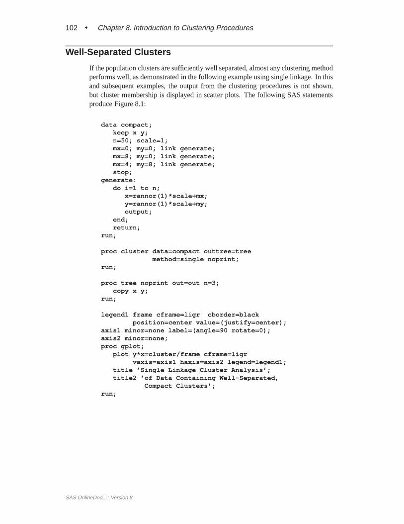
Well-Separated Clusters
If the population clusters are sufficiently well separated, almost any clustering methodperforms well, as demonstrated in the following example using single linkage. In thisand subsequent examples, the output from the clustering procedures is not shown,but cluster membership is displayed in scatter plots. The following SAS statementsproduce Figure 8.1:
data compact;keep x y;n=50; scale=1;mx=0; my=0; link generate;mx=8; my=0; link generate;mx=4; my=8; link generate;stop;
generate:do i=1 to n;
x=rannor(1)*scale+mx;y=rannor(1)*scale+my;output;
end;return;
run;
proc cluster data=compact outtree=treemethod=single noprint;
run;
proc tree noprint out=out n=3;copy x y;
run;
legend1 frame cframe=ligr cborder=blackposition=center value=(justify=center);
axis1 minor=none label=(angle=90 rotate=0);axis2 minor=none;proc gplot;
plot y*x=cluster/frame cframe=ligrvaxis=axis1 haxis=axis2 legend=legend1;
title ’Single Linkage Cluster Analysis’;title2 ’of Data Containing Well-Separated,
Compact Clusters’;run;
SAS OnlineDoc: Version 8
Poorly Separated Clusters � 103
Figure 8.1. Data Containing Well-Separated, Compact Clusters: PROC CLUSTERwith METHOD=SINGLE and PROC GPLOT
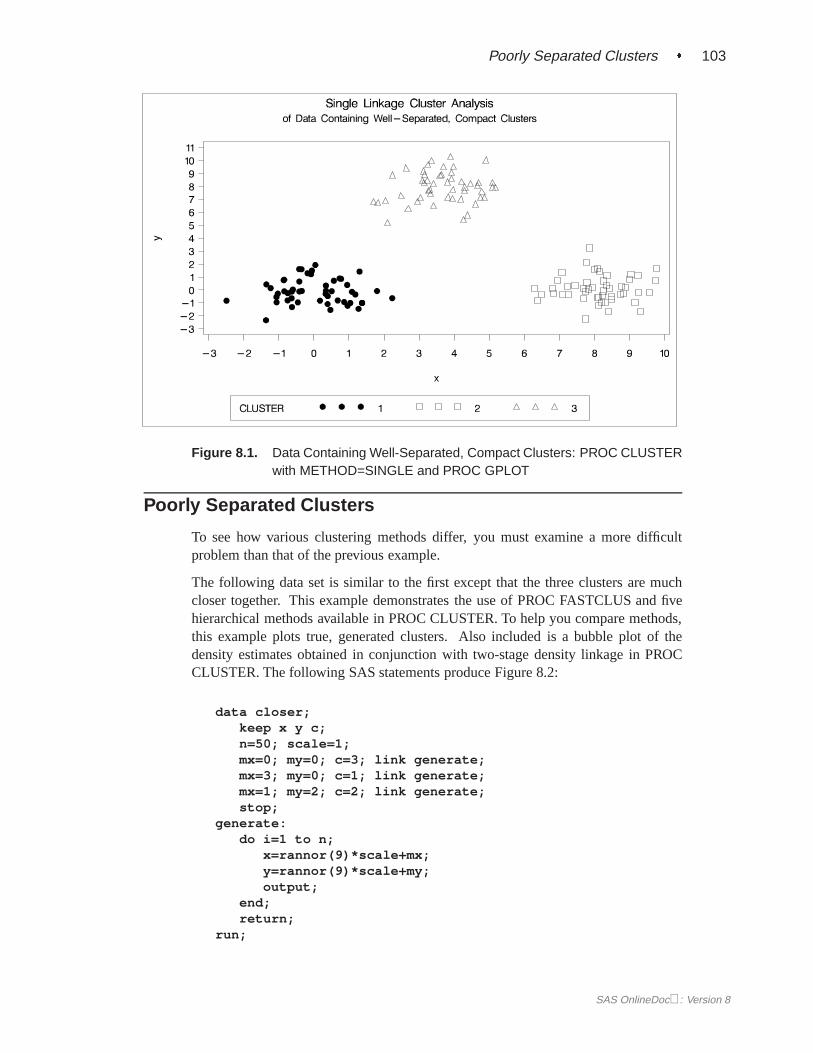
Poorly Separated Clusters
To see how various clustering methods differ, you must examine a more difficultproblem than that of the previous example.
The following data set is similar to the first except that the three clusters are muchcloser together. This example demonstrates the use of PROC FASTCLUS and fivehierarchical methods available in PROC CLUSTER. To help you compare methods,this example plots true, generated clusters. Also included is a bubble plot of thedensity estimates obtained in conjunction with two-stage density linkage in PROCCLUSTER. The following SAS statements produce Figure 8.2:
data closer;keep x y c;n=50; scale=1;mx=0; my=0; c=3; link generate;mx=3; my=0; c=1; link generate;mx=1; my=2; c=2; link generate;stop;
generate:do i=1 to n;
x=rannor(9)*scale+mx;y=rannor(9)*scale+my;output;
end;return;
run;
SAS OnlineDoc: Version 8

104 � Chapter 8. Introduction to Clustering Procedures
title ’True Clusters for Data Containing Poorly Separated,Compact Clusters’;
proc gplot;plot y*x=c/frame cframe=ligr
vaxis=axis1 haxis=axis2 legend=legend1;run;
Figure 8.2. Data Containing Poorly Separated, Compact Clusters: Plot of TrueClusters
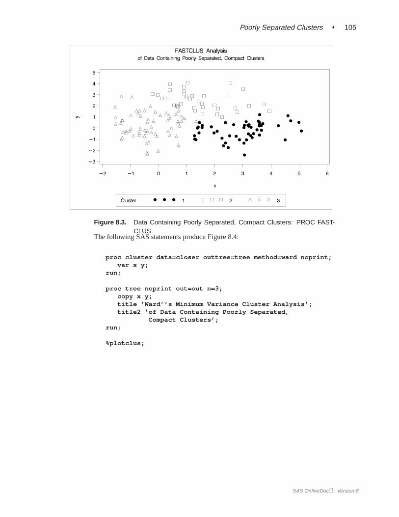
The following statements use the FASTCLUS procedure to find three clusters andthe GPLOT procedure to plot the clusters. Since the GPLOT step is repeated sev-eral times in this example, it is contained in the PLOTCLUS macro. The followingstatements produce Figure 8.3.
%macro plotclus;legend1 frame cframe=ligr cborder=black
position=center value=(justify=center);axis1 minor=none label=(angle=90 rotate=0);axis2 minor=none;proc gplot;
plot y*x=cluster/frame cframe=ligrvaxis=axis1 haxis=axis2 legend=legend1;
run;%mend plotclus;
proc fastclus data=closer out=out maxc=3 noprint;var x y;title ’FASTCLUS Analysis’;title2 ’of Data Containing Poorly Separated,
Compact Clusters’;run;%plotclus;
SAS OnlineDoc: Version 8
Poorly Separated Clusters � 105
Figure 8.3. Data Containing Poorly Separated, Compact Clusters: PROC FAST-CLUS
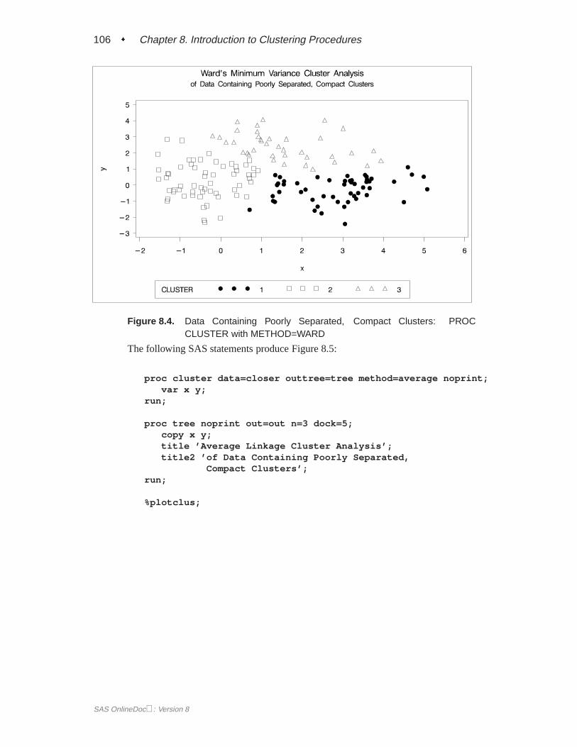
The following SAS statements produce Figure 8.4:
proc cluster data=closer outtree=tree method=ward noprint;var x y;
run;
proc tree noprint out=out n=3;copy x y;title ’Ward’’s Minimum Variance Cluster Analysis’;title2 ’of Data Containing Poorly Separated,
Compact Clusters’;run;
%plotclus;
SAS OnlineDoc: Version 8
106 � Chapter 8. Introduction to Clustering Procedures
Figure 8.4. Data Containing Poorly Separated, Compact Clusters: PROCCLUSTER with METHOD=WARD
The following SAS statements produce Figure 8.5:
proc cluster data=closer outtree=tree method=average noprint;var x y;
run;
proc tree noprint out=out n=3 dock=5;copy x y;title ’Average Linkage Cluster Analysis’;title2 ’of Data Containing Poorly Separated,
Compact Clusters’;run;
%plotclus;
SAS OnlineDoc: Version 8
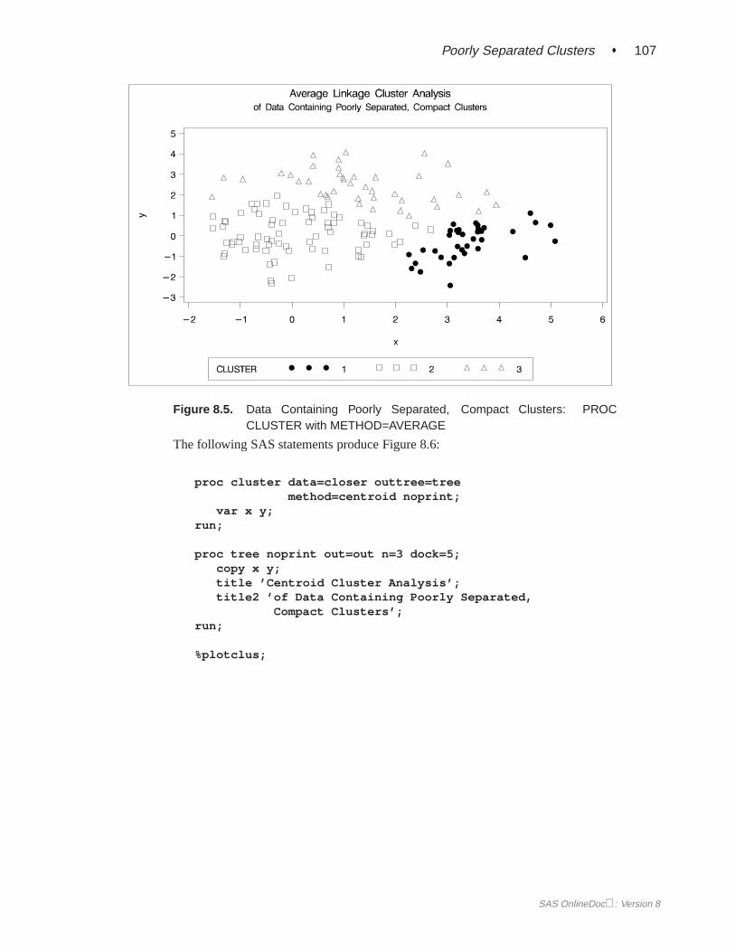
Poorly Separated Clusters � 107
Figure 8.5. Data Containing Poorly Separated, Compact Clusters: PROCCLUSTER with METHOD=AVERAGE
The following SAS statements produce Figure 8.6:
proc cluster data=closer outtree=treemethod=centroid noprint;
var x y;run;
proc tree noprint out=out n=3 dock=5;copy x y;title ’Centroid Cluster Analysis’;title2 ’of Data Containing Poorly Separated,
Compact Clusters’;run;
%plotclus;
SAS OnlineDoc: Version 8
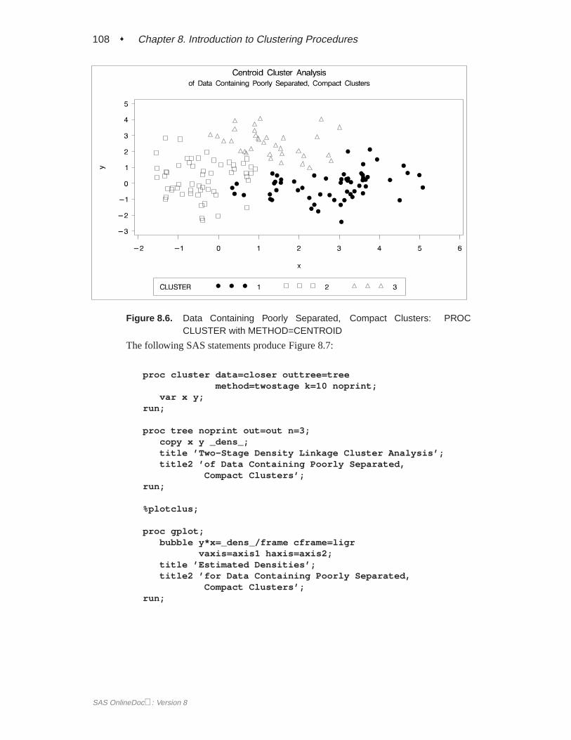
108 � Chapter 8. Introduction to Clustering Procedures
Figure 8.6. Data Containing Poorly Separated, Compact Clusters: PROCCLUSTER with METHOD=CENTROID
The following SAS statements produce Figure 8.7:
proc cluster data=closer outtree=treemethod=twostage k=10 noprint;
var x y;run;
proc tree noprint out=out n=3;copy x y _dens_;title ’Two-Stage Density Linkage Cluster Analysis’;title2 ’of Data Containing Poorly Separated,
Compact Clusters’;run;
%plotclus;
proc gplot;bubble y*x=_dens_/frame cframe=ligr
vaxis=axis1 haxis=axis2;title ’Estimated Densities’;title2 ’for Data Containing Poorly Separated,
Compact Clusters’;run;
SAS OnlineDoc: Version 8

Poorly Separated Clusters � 109
Figure 8.7. Data Containing Poorly Separated, Compact Clusters: PROCCLUSTER with METHOD=TWOSTAGE
SAS OnlineDoc: Version 8
110 � Chapter 8. Introduction to Clustering Procedures
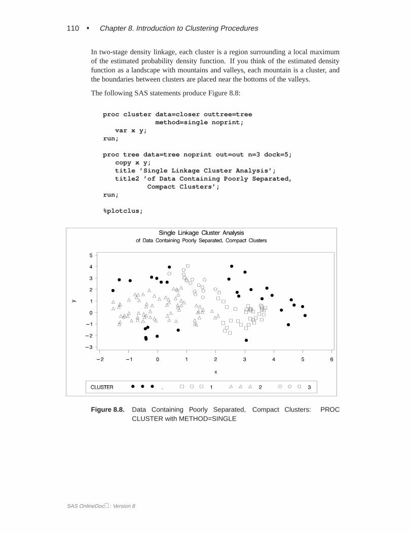
In two-stage density linkage, each cluster is a region surrounding a local maximumof the estimated probability density function. If you think of the estimated densityfunction as a landscape with mountains and valleys, each mountain is a cluster, andthe boundaries between clusters are placed near the bottoms of the valleys.
The following SAS statements produce Figure 8.8:
proc cluster data=closer outtree=treemethod=single noprint;
var x y;run;
proc tree data=tree noprint out=out n=3 dock=5;copy x y;title ’Single Linkage Cluster Analysis’;title2 ’of Data Containing Poorly Separated,
Compact Clusters’;run;
%plotclus;
Figure 8.8. Data Containing Poorly Separated, Compact Clusters: PROCCLUSTER with METHOD=SINGLE
SAS OnlineDoc: Version 8
Multinormal Clusters of Unequal Size and Dispersion � 111
The two least-squares methods, PROC FASTCLUS and Ward’s, yield the most uni-form cluster sizes and the best recovery of the true clusters. This result is expectedsince these two methods are biased toward recovering compact clusters of equal size.With average linkage, the lower-left cluster is too large; with the centroid method, thelower-right cluster is too large; and with two-stage density linkage, the top cluster istoo large. The single linkage analysis resembles average linkage except for the largenumber of outliers resulting from the DOCK= option in the PROC TREE statement;the outliers are plotted as dots (missing values).
Multinormal Clusters of Unequal Size and Dispersion
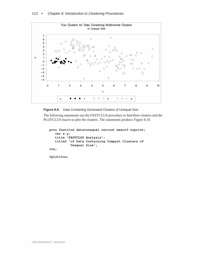
In this example, there are three multinormal clusters that differ in size and dispersion.PROC FASTCLUS and five of the hierarchical methods available in PROC CLUS-TER are used. To help you compare methods, the true, generated clusters are plotted.The following SAS statements produce Figure 8.9:
data unequal;keep x y c;mx=1; my=0; n=20; scale=.5; c=1; link generate;mx=6; my=0; n=80; scale=2.; c=3; link generate;mx=3; my=4; n=40; scale=1.; c=2; link generate;stop;
generate:do i=1 to n;
x=rannor(1)*scale+mx;y=rannor(1)*scale+my;output;
end;return;
run;
title ’True Clusters for Data Containing MultinormalClusters’;
title2 ’of Unequal Size’;proc gplot;
plot y*x=c/frame cframe=ligrvaxis=axis1 haxis=axis2 legend=legend1;
run;
SAS OnlineDoc: Version 8
112 � Chapter 8. Introduction to Clustering Procedures
Figure 8.9. Data Containing Generated Clusters of Unequal Size
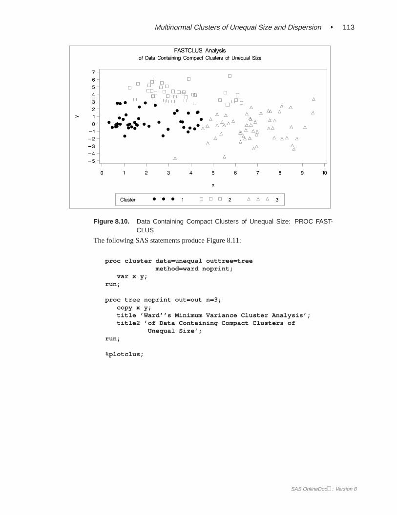
The following statements use the FASTCLUS procedure to find three clusters and thePLOTCLUS macro to plot the clusters. The statements produce Figure 8.10.
proc fastclus data=unequal out=out maxc=3 noprint;var x y;title ’FASTCLUS Analysis’;title2 ’of Data Containing Compact Clusters of
Unequal Size’;run;
%plotclus;
SAS OnlineDoc: Version 8
Multinormal Clusters of Unequal Size and Dispersion � 113
Figure 8.10. Data Containing Compact Clusters of Unequal Size: PROC FAST-CLUS
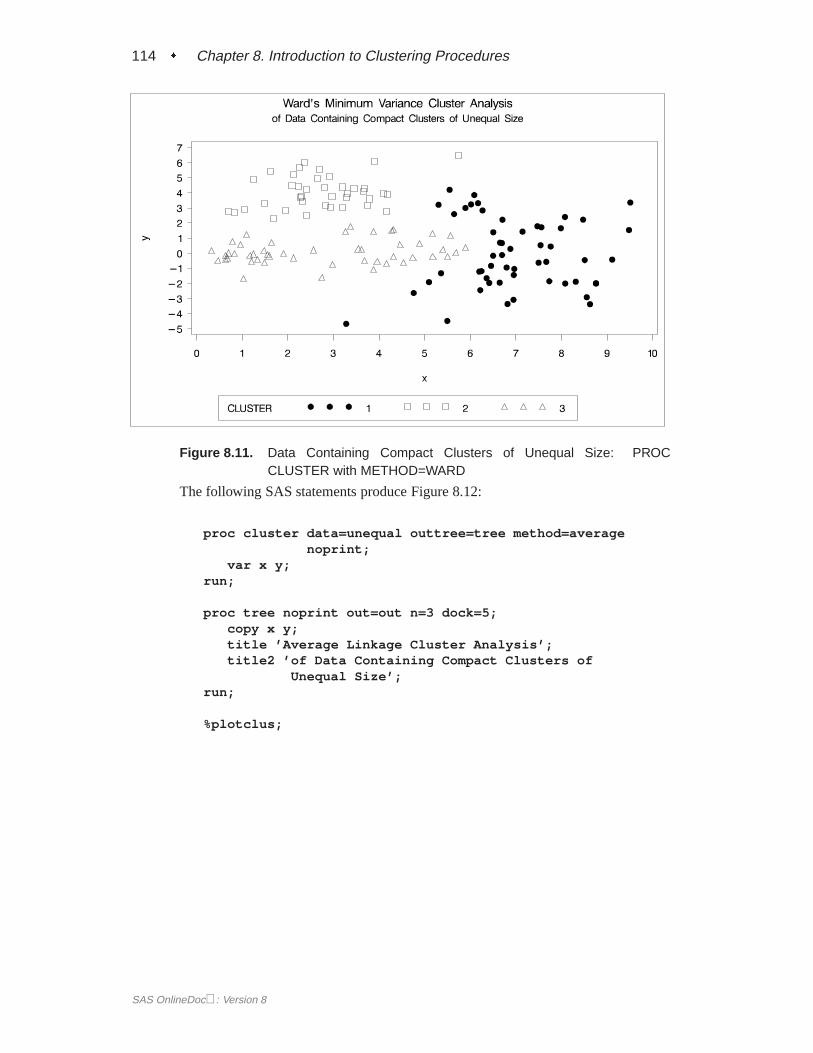
The following SAS statements produce Figure 8.11:
proc cluster data=unequal outtree=treemethod=ward noprint;
var x y;run;
proc tree noprint out=out n=3;copy x y;title ’Ward’’s Minimum Variance Cluster Analysis’;title2 ’of Data Containing Compact Clusters of
Unequal Size’;run;
%plotclus;
SAS OnlineDoc: Version 8
114 � Chapter 8. Introduction to Clustering Procedures
Figure 8.11. Data Containing Compact Clusters of Unequal Size: PROCCLUSTER with METHOD=WARD
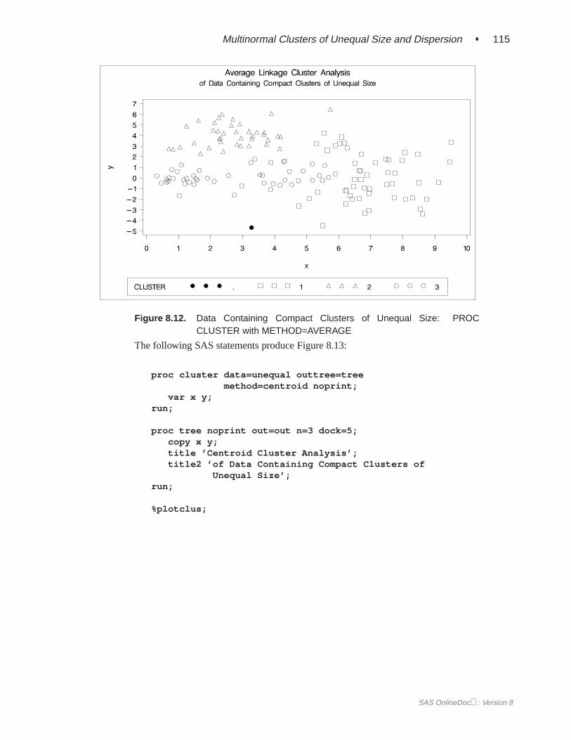
The following SAS statements produce Figure 8.12:
proc cluster data=unequal outtree=tree method=averagenoprint;
var x y;run;
proc tree noprint out=out n=3 dock=5;copy x y;title ’Average Linkage Cluster Analysis’;title2 ’of Data Containing Compact Clusters of
Unequal Size’;run;
%plotclus;
SAS OnlineDoc: Version 8
Multinormal Clusters of Unequal Size and Dispersion � 115
Figure 8.12. Data Containing Compact Clusters of Unequal Size: PROCCLUSTER with METHOD=AVERAGE
The following SAS statements produce Figure 8.13:
proc cluster data=unequal outtree=treemethod=centroid noprint;
var x y;run;
proc tree noprint out=out n=3 dock=5;copy x y;title ’Centroid Cluster Analysis’;title2 ’of Data Containing Compact Clusters of
Unequal Size’;run;
%plotclus;
SAS OnlineDoc: Version 8
116 � Chapter 8. Introduction to Clustering Procedures
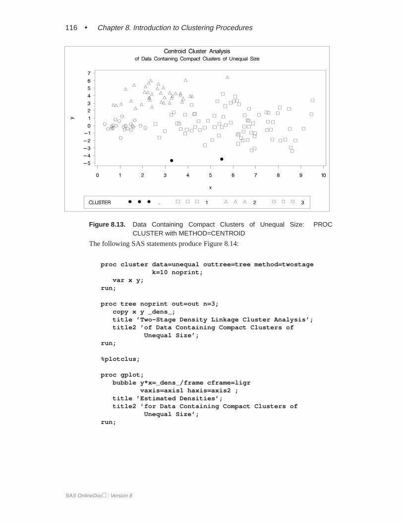
Figure 8.13. Data Containing Compact Clusters of Unequal Size: PROCCLUSTER with METHOD=CENTROID
The following SAS statements produce Figure 8.14:
proc cluster data=unequal outtree=tree method=twostagek=10 noprint;
var x y;run;
proc tree noprint out=out n=3;copy x y _dens_;title ’Two-Stage Density Linkage Cluster Analysis’;title2 ’of Data Containing Compact Clusters of
Unequal Size’;run;
%plotclus;
proc gplot;bubble y*x=_dens_/frame cframe=ligr
vaxis=axis1 haxis=axis2 ;title ’Estimated Densities’;title2 ’for Data Containing Compact Clusters of
Unequal Size’;run;
SAS OnlineDoc: Version 8

Multinormal Clusters of Unequal Size and Dispersion � 117
Figure 8.14. Data Containing Compact Clusters of Unequal Size: PROCCLUSTER with METHOD=TWOSTAGE
SAS OnlineDoc: Version 8
118 � Chapter 8. Introduction to Clustering Procedures
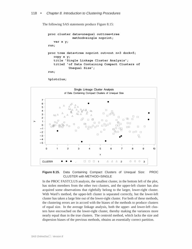
The following SAS statements produce Figure 8.15:
proc cluster data=unequal outtree=treemethod=single noprint;
var x y;run;
proc tree data=tree noprint out=out n=3 dock=5;copy x y;title ’Single Linkage Cluster Analysis’;title2 ’of Data Containing Compact Clusters of
Unequal Size’;run;
%plotclus;
Figure 8.15. Data Containing Compact Clusters of Unequal Size: PROCCLUSTER with METHOD=SINGLE
In the PROC FASTCLUS analysis, the smallest cluster, in the bottom left of the plot,has stolen members from the other two clusters, and the upper-left cluster has alsoacquired some observations that rightfully belong to the larger, lower-right cluster.With Ward’s method, the upper-left cluster is separated correctly, but the lower-leftcluster has taken a large bite out of the lower-right cluster. For both of these methods,the clustering errors are in accord with the biases of the methods to produce clustersof equal size. In the average linkage analysis, both the upper- and lower-left clus-ters have encroached on the lower-right cluster, thereby making the variances morenearly equal than in the true clusters. The centroid method, which lacks the size anddispersion biases of the previous methods, obtains an essentially correct partition.
SAS OnlineDoc: Version 8
Elongated Multinormal Clusters � 119
Two-stage density linkage does almost as well even though the compact shapes ofthese clusters favor the traditional methods. Single linkage also produces excellentresults.
Elongated Multinormal Clusters
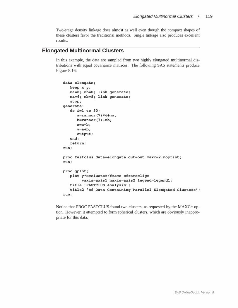
In this example, the data are sampled from two highly elongated multinormal dis-tributions with equal covariance matrices. The following SAS statements produceFigure 8.16:
data elongate;keep x y;ma=8; mb=0; link generate;ma=6; mb=8; link generate;stop;
generate:do i=1 to 50;
a=rannor(7)*6+ma;b=rannor(7)+mb;x=a-b;y=a+b;output;
end;return;
run;
proc fastclus data=elongate out=out maxc=2 noprint;run;
proc gplot;plot y*x=cluster/frame cframe=ligr
vaxis=axis1 haxis=axis2 legend=legend1;title ’FASTCLUS Analysis’;title2 ’of Data Containing Parallel Elongated Clusters’;
run;
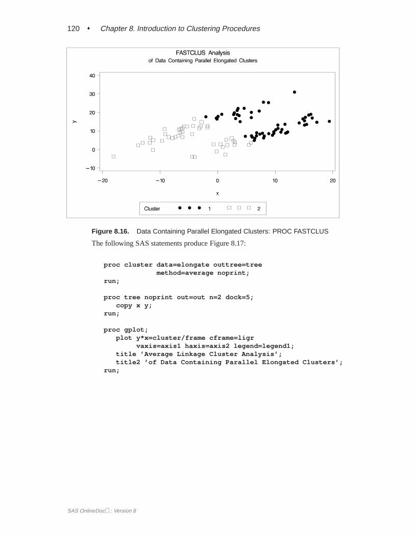
Notice that PROC FASTCLUS found two clusters, as requested by the MAXC= op-tion. However, it attempted to form spherical clusters, which are obviously inappro-priate for this data.
SAS OnlineDoc: Version 8
120 � Chapter 8. Introduction to Clustering Procedures
Figure 8.16. Data Containing Parallel Elongated Clusters: PROC FASTCLUS
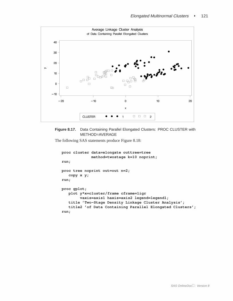
The following SAS statements produce Figure 8.17:
proc cluster data=elongate outtree=treemethod=average noprint;
run;
proc tree noprint out=out n=2 dock=5;copy x y;
run;
proc gplot;plot y*x=cluster/frame cframe=ligr
vaxis=axis1 haxis=axis2 legend=legend1;title ’Average Linkage Cluster Analysis’;title2 ’of Data Containing Parallel Elongated Clusters’;
run;
SAS OnlineDoc: Version 8
Elongated Multinormal Clusters � 121
Figure 8.17. Data Containing Parallel Elongated Clusters: PROC CLUSTER withMETHOD=AVERAGE
The following SAS statements produce Figure 8.18:
proc cluster data=elongate outtree=treemethod=twostage k=10 noprint;
run;
proc tree noprint out=out n=2;copy x y;
run;
proc gplot;plot y*x=cluster/frame cframe=ligr
vaxis=axis1 haxis=axis2 legend=legend1;title ’Two-Stage Density Linkage Cluster Analysis’;title2 ’of Data Containing Parallel Elongated Clusters’;
run;
SAS OnlineDoc: Version 8

122 � Chapter 8. Introduction to Clustering Procedures
Figure 8.18. Data Containing Parallel Elongated Clusters: PROC CLUSTER withMETHOD=TWOSTAGE
PROC FASTCLUS and average linkage fail miserably. Ward’s method and the cen-troid method, not shown, produce almost the same results. Two-stage density link-age, however, recovers the correct clusters. Single linkage, not shown, finds the sameclusters as two-stage density linkage except for some outliers.
In this example, the population clusters have equal covariance matrices. If the within-cluster covariances are known, the data can be transformed to make the clusters spher-ical so that any of the clustering methods can find the correct clusters. But whenyou are doing a cluster analysis, you do not know what the true clusters are, so youcannot calculate the within-cluster covariance matrix. Nevertheless, it is sometimespossible to estimate the within-cluster covariance matrix without knowing the clus-ter membership or even the number of clusters, using an approach invented by Art,Gnanadesikan, and Kettenring (1982). A method for obtaining such an estimate isavailable in the ACECLUS procedure.
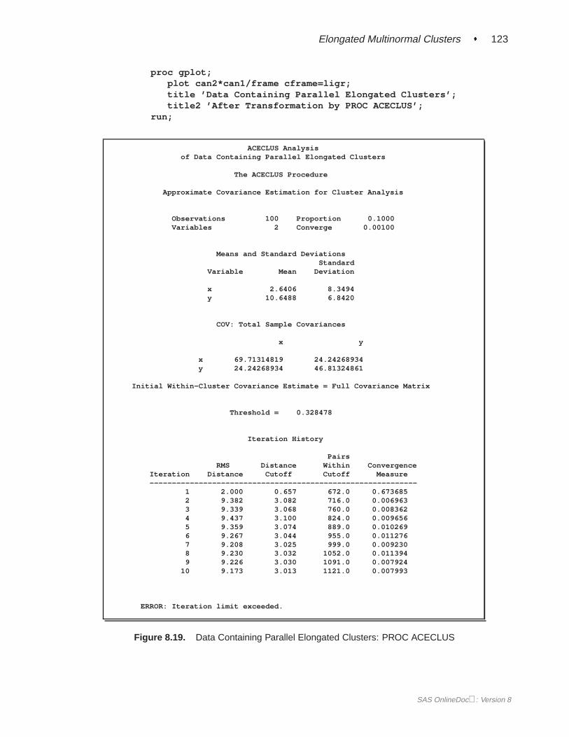
In the following analysis, PROC ACECLUS transforms the variables X and Y intocanonical variables CAN1 and CAN2. The latter are plotted and then used in a clusteranalysis by Ward’s method. The clusters are then plotted with the original variablesX and Y. The following SAS statements produce Figure 8.19:
proc aceclus data=elongate out=ace p=.1;var x y;title ’ACECLUS Analysis’;title2 ’of Data Containing Parallel Elongated Clusters’;
run;
SAS OnlineDoc: Version 8
Elongated Multinormal Clusters � 123
proc gplot;plot can2*can1/frame cframe=ligr;title ’Data Containing Parallel Elongated Clusters’;title2 ’After Transformation by PROC ACECLUS’;
run;
ACECLUS Analysisof Data Containing Parallel Elongated Clusters
The ACECLUS Procedure
Approximate Covariance Estimation for Cluster Analysis
Observations 100 Proportion 0.1000Variables 2 Converge 0.00100
Means and Standard DeviationsStandard
Variable Mean Deviation
x 2.6406 8.3494y 10.6488 6.8420
COV: Total Sample Covariances
x y
x 69.71314819 24.24268934y 24.24268934 46.81324861
Initial Within-Cluster Covariance Estimate = Full Covariance Matrix
Threshold = 0.328478
Iteration History
PairsRMS Distance Within Convergence
Iteration Distance Cutoff Cutoff Measure------------------------------------------------------------
1 2.000 0.657 672.0 0.6736852 9.382 3.082 716.0 0.0069633 9.339 3.068 760.0 0.0083624 9.437 3.100 824.0 0.0096565 9.359 3.074 889.0 0.0102696 9.267 3.044 955.0 0.0112767 9.208 3.025 999.0 0.0092308 9.230 3.032 1052.0 0.0113949 9.226 3.030 1091.0 0.007924
10 9.173 3.013 1121.0 0.007993
ERROR: Iteration limit exceeded.
Figure 8.19. Data Containing Parallel Elongated Clusters: PROC ACECLUS
SAS OnlineDoc: Version 8

124 � Chapter 8. Introduction to Clustering Procedures
ACECLUS Analysisof Data Containing Parallel Elongated Clusters
The ACECLUS Procedure
ACE: Approximate Covariance Estimate Within Clusters
x y
x 9.299329632 8.215362614y 8.215362614 8.937753936
Eigenvalues of Inv(ACE)*(COV-ACE)
Eigenvalue Difference Proportion Cumulative
1 36.7091 33.1672 0.9120 0.91202 3.5420 0.0880 1.0000
Eigenvectors (Raw Canonical Coefficients)
Can1 Can2
x -.748392 0.109547y 0.736349 0.230272
Standardized Canonical Coefficients
Can1 Can2
x -6.24866 0.91466y 5.03812 1.57553
Figure 8.20. Data Containing Parallel Elongated Clusters After Transformation byPROC ACECLUS
SAS OnlineDoc: Version 8
Nonconvex Clusters � 125
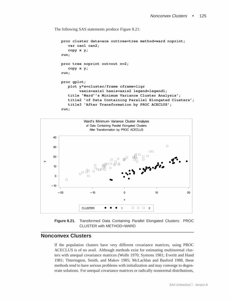
The following SAS statements produce Figure 8.21:
proc cluster data=ace outtree=tree method=ward noprint;var can1 can2;copy x y;
run;
proc tree noprint out=out n=2;copy x y;
run;
proc gplot;plot y*x=cluster/frame cframe=ligr
vaxis=axis1 haxis=axis2 legend=legend1;title ’Ward’’s Minimum Variance Cluster Analysis’;title2 ’of Data Containing Parallel Elongated Clusters’;title3 ’After Transformation by PROC ACECLUS’;
run;
Figure 8.21. Transformed Data Containing Parallel Elongated Clusters: PROCCLUSTER with METHOD=WARD
Nonconvex Clusters
If the population clusters have very different covariance matrices, using PROCACECLUS is of no avail. Although methods exist for estimating multinormal clus-ters with unequal covariance matrices (Wolfe 1970; Symons 1981; Everitt and Hand1981; Titterington, Smith, and Makov 1985; McLachlan and Basford 1988, thesemethods tend to have serious problems with initialization and may converge to degen-erate solutions. For unequal covariance matrices or radically nonnormal distributions,
SAS OnlineDoc: Version 8
126 � Chapter 8. Introduction to Clustering Procedures
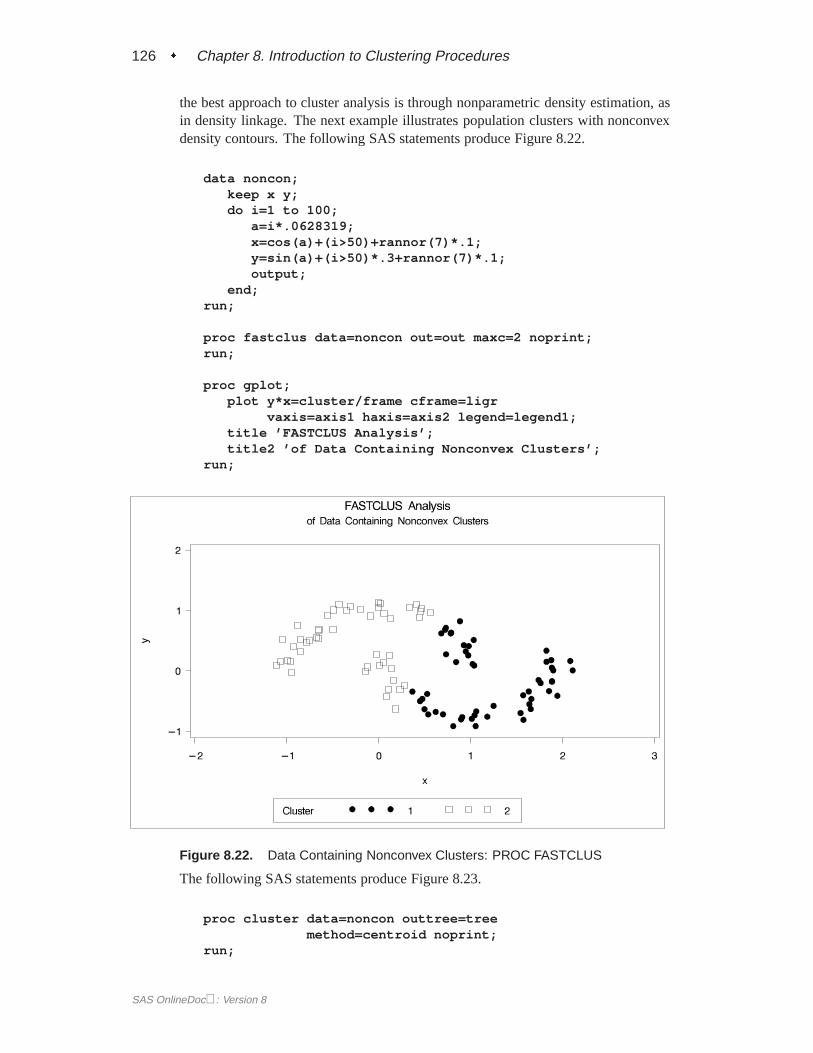
the best approach to cluster analysis is through nonparametric density estimation, asin density linkage. The next example illustrates population clusters with nonconvexdensity contours. The following SAS statements produce Figure 8.22.
data noncon;keep x y;do i=1 to 100;
a=i*.0628319;x=cos(a)+(i>50)+rannor(7)*.1;y=sin(a)+(i>50)*.3+rannor(7)*.1;output;
end;run;
proc fastclus data=noncon out=out maxc=2 noprint;run;
proc gplot;plot y*x=cluster/frame cframe=ligr
vaxis=axis1 haxis=axis2 legend=legend1;title ’FASTCLUS Analysis’;title2 ’of Data Containing Nonconvex Clusters’;
run;
Figure 8.22. Data Containing Nonconvex Clusters: PROC FASTCLUS
The following SAS statements produce Figure 8.23.
proc cluster data=noncon outtree=treemethod=centroid noprint;
run;
SAS OnlineDoc: Version 8
Nonconvex Clusters � 127
proc tree noprint out=out n=2 dock=5;copy x y;
run;
proc gplot;plot y*x=cluster/frame cframe=ligr
vaxis=axis1 haxis=axis2 legend=legend1;title ’Centroid Cluster Analysis’;title2 ’of Data Containing Nonconvex Clusters’;
run;
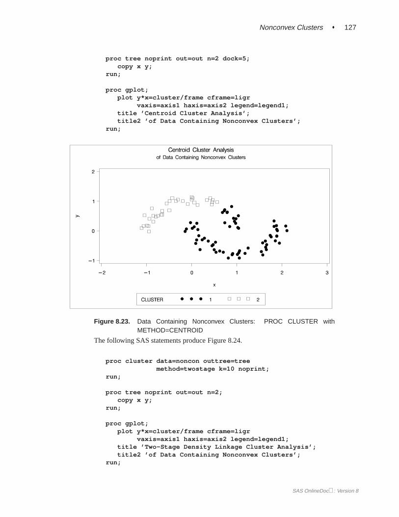
Figure 8.23. Data Containing Nonconvex Clusters: PROC CLUSTER withMETHOD=CENTROID
The following SAS statements produce Figure 8.24.
proc cluster data=noncon outtree=treemethod=twostage k=10 noprint;
run;
proc tree noprint out=out n=2;copy x y;
run;
proc gplot;plot y*x=cluster/frame cframe=ligr
vaxis=axis1 haxis=axis2 legend=legend1;title ’Two-Stage Density Linkage Cluster Analysis’;title2 ’of Data Containing Nonconvex Clusters’;
run;
SAS OnlineDoc: Version 8
128 � Chapter 8. Introduction to Clustering Procedures
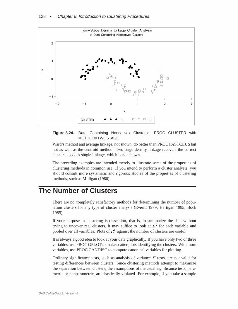
Figure 8.24. Data Containing Nonconvex Clusters: PROC CLUSTER withMETHOD=TWOSTAGE
Ward’s method and average linkage, not shown, do better than PROC FASTCLUS butnot as well as the centroid method. Two-stage density linkage recovers the correctclusters, as does single linkage, which is not shown.
The preceding examples are intended merely to illustrate some of the properties ofclustering methods in common use. If you intend to perform a cluster analysis, youshould consult more systematic and rigorous studies of the properties of clusteringmethods, such as Milligan (1980).
The Number of Clusters
There are no completely satisfactory methods for determining the number of popu-lation clusters for any type of cluster analysis (Everitt 1979; Hartigan 1985; Bock1985).
If your purpose in clustering is dissection, that is, to summarize the data withouttrying to uncover real clusters, it may suffice to look atR2 for each variable andpooled over all variables. Plots ofR2 against the number of clusters are useful.
It is always a good idea to look at your data graphically. If you have only two or threevariables, use PROC GPLOT to make scatter plots identifying the clusters. With morevariables, use PROC CANDISC to compute canonical variables for plotting.
Ordinary significance tests, such as analysis of varianceF tests, are not valid fortesting differences between clusters. Since clustering methods attempt to maximizethe separation between clusters, the assumptions of the usual significance tests, para-metric or nonparametric, are drastically violated. For example, if you take a sample
SAS OnlineDoc: Version 8

The Number of Clusters � 129
of 100 observations from a single univariate normal distribution, have PROC FAST-CLUS divide it into two clusters, and run at test between the clusters, you usuallyobtain ap-value of less than 0.0001. For the same reason, methods that purport to testfor clusters against the null hypothesis that objects are assigned randomly to clusters(such as McClain and Rao 1975; Klastorin 1983) are useless.
Most valid tests for clusters either have intractable sampling distributions or involvenull hypotheses for which rejection is uninformative. For clustering methods basedon distance matrices, a popular null hypothesis is that all permutations of the valuesin the distance matrix are equally likely (Ling 1973; Hubert 1974). Using this nullhypothesis, you can do a permutation test or a rank test. The trouble with the permu-tation hypothesis is that, with any real data, the null hypothesis is implausible even ifthe data do not contain clusters. Rejecting the null hypothesis does not provide anyuseful information (Hubert and Baker 1977).
Another common null hypothesis is that the data are a random sample from a multi-variate normal distribution (Wolfe 1970, 1978; Duda and Hart 1973; Lee 1979). Themultivariate normal null hypothesis arises naturally in normal mixture models (Titter-ington, Smith, and Makov 1985; McLachlan and Basford 1988). Unfortunately, thelikelihood ratio test statistic does not have the usual asymptotic chi-squared distribu-tion because the regularity conditions do not hold. Approximations to the asymptoticdistribution of the likelihood ratio have been suggested (Wolfe 1978), but the ade-quacy of these approximations is debatable (Everitt 1981; Thode, Mendell, and Finch1988). For small samples, bootstrapping seems preferable (McLachlan and Basford1988). Bayesian inference provides a promising alternative to likelihood ratio testsfor the number of mixture components for both normal mixtures and other types ofdistributions (Binder 1978, 1981; Banfield and Raftery 1993; Bensmail et al. 1997).
The multivariate normal null hypothesis is better than the permutation null hypoth-esis, but it is not satisfactory because there is typically a high probability of rejec-tion if the data are sampled from a distribution with lower kurtosis than a normaldistribution, such as a uniform distribution. The tables in Englemann and Hartigan(1969), for example, generally lead to rejection of the null hypothesis when the dataare sampled from a uniform distribution. Hawkins, Muller, and ten Krooden (1982,pp. 337–340) discuss a highly conservative Bonferroni method for hypothesis test-ing. The conservativeness of this approach may compensate to some extent for theliberalness exhibited by tests based on normal distributions when the population isuniform.
Perhaps a better null hypothesis is that the data are sampled from a uniform distribu-tion (Hartigan 1978; Arnold 1979; Sarle 1983). The uniform null hypothesis leads toconservative error rates when the data are sampled from a strongly unimodal distri-bution such as the normal. However, in two or more dimensions and depending onthe test statistic, the results can be very sensitive to the shape of the region of sup-port of the uniform distribution. Sarle (1983) suggests using a hyperbox with sidesproportional in length to the singular values of the centered coordinate matrix.
SAS OnlineDoc: Version 8
130 � Chapter 8. Introduction to Clustering Procedures
Given that the uniform distribution provides an appropriate null hypothesis, thereare still serious difficulties in obtaining sampling distributions. Some asymptoticresults are available (Hartigan 1978, 1985; Pollard 1981; Bock 1985) for the within-cluster sum of squares, the criterion that PROC FASTCLUS and Ward’s minimumvariance method attempt to optimize. No distributional theory for finite sample sizeshas yet appeared. Currently, the only practical way to obtain sampling distributionsfor realistic sample sizes is by computer simulation.
Arnold (1979) used simulation to derive tables of the distribution of a criterion basedon the determinant of the within-cluster sum of squares matrixjWj. Both nor-mal and uniform null distributions were used. Having obtained clusters with eitherPROC FASTCLUS or PROC CLUSTER, you can compute Arnold’s criterion withthe ANOVA or CANDISC procedure. Arnold’s tables provide a conservative test be-cause PROC FASTCLUS and PROC CLUSTER attempt to minimize the trace ofW
rather than the determinant. Marriott (1971, 1975) also provides useful informationon jWj as a criterion for the number of clusters.
Sarle (1983) used extensive simulations to develop the cubic clustering criterion(CCC), which can be used for crude hypothesis testing and estimating the numberof population clusters. The CCC is based on the assumption that a uniform distribu-tion on a hyperrectangle will be divided into clusters shaped roughly like hypercubes.In large samples that can be divided into the appropriate number of hypercubes, thisassumption gives very accurate results. In other cases the approximation is generallyconservative. For details about the interpretation of the CCC, consult Sarle (1983).
Milligan and Cooper (1985) and Cooper and Milligan (1988) compared thirty meth-ods for estimating the number of population clusters using four hierarchical cluster-ing methods. The three criteria that performed best in these simulation studies with ahigh degree of error in the data were a pseudoF statistic developed by Calinski andHarabasz (1974), a statistic referred to asJe(2)=Je(1) by Duda and Hart (1973) thatcan be transformed into a pseudot2 statistic, and the cubic clustering criterion. ThepseudoF statistic and the CCC are displayed by PROC FASTCLUS; these two statis-tics and the pseudot2 statistic, which can be applied only to hierarchical methods,are displayed by PROC CLUSTER. It may be advisable to look for consensus amongthe three statistics, that is, local peaks of the CCC and pseudoF statistic combinedwith a small value of the pseudot2 statistic and a larger pseudot2 for the next clusterfusion. It must be emphasized that these criteria are appropriate only for compact orslightly elongated clusters, preferably clusters that are roughly multivariate normal.
Recent research has tended to de-emphasize mixture models in favor of nonparamet-ric models in which clusters correspond to modes in the probability density function.Hartigan and Hartigan (1985) and Hartigan (1985) developed a test of unimodalityversus bimodality in the univariate case.
Nonparametric tests for the number of clusters can also be based on nonparametricdensity estimates. This approach requires much weaker assumptions than mixturemodels, namely, that the observations are sampled independently and that the distri-bution can be estimated nonparametrically. Silverman (1986) describes a bootstraptest for the number of modes using a Gaussian kernel density estimate, but problemshave been reported with this method under the uniform null distribution. Further
SAS OnlineDoc: Version 8
References � 131
developments in nonparametric methods are given by Mueller and Sawitzki (1991),Minnotte (1992), and Polonik (1993). All of these methods suffer from heavy com-putational requirements.
One useful descriptive approach to the number-of-clusters problem is provided byWong and Schaack (1982), based on akth-nearest-neighbor density estimate. Thekth-nearest-neighbor clustering method developed by Wong and Lane (1983) is ap-plied with varying values ofk. Each value ofk yields an estimate of the number ofmodal clusters. If the estimated number of modal clusters is constant for a wide rangeof k values, there is strong evidence of at least that many modes in the population. Aplot of the estimated number of modes againstk can be highly informative. Attemptsto derive a formal hypothesis test from this diagnostic plot have met with difficulties,but a simulation approach similar to Silverman’s (1986) does seem to work (Girman1994). The simulation, of course, requires considerable computer time.
Sarle and Kuo (1993) document a less expensive approximate nonparametric test forthe number of clusters that has been implemented in the MODECLUS procedure.This test sacrifices statistical efficiency for computational efficiency. The method forconducting significance tests is described in the chapter on the MODECLUS proce-dure. This method has the following useful features:
� No distributional assumptions are required.
� The choice of smoothing parameter is not critical since you can try any numberof different values.
� The data can be coordinates or distances.
� Time and space requirements for the significance tests are no worse than thosefor obtaining the clusters.
� The power is high enough to be useful for practical purposes.
The method for computing thep-values is based on a series of plausible approxima-tions. There are as yet no rigorous proofs that the method is infallible. Neither arethere any asymptotic results. However, simulations for sample sizes ranging from20 to 2000 indicate that thep-values are almost always conservative. The only casediscovered so far in which thep-values are liberal is a uniform distribution in onedimension for which the simulated error rates exceed the nominal significance levelonly slightly for a limited range of sample sizes.
References
Anderberg, M.R. (1973),Cluster Analysis for Applications, New York: AcademicPress, Inc.
Arnold, S.J. (1979), “A Test for Clusters,”Journal of Marketing Research,16,545–551.
Art, D., Gnanadesikan, R., and Kettenring, R. (1982), “Data-based Metrics for Clus-ter Analysis,”Utilitas Mathematica, 21A, 75–99.
SAS OnlineDoc: Version 8
132 � Chapter 8. Introduction to Clustering Procedures
Banfield, J.D. and Raftery, A.E. (1993), “Model-Based Gaussian and Non-GaussianClustering,”Biometrics, 49, 803–821.
Bensmail, H., Celeux, G., Raftery, A.E., and Robert, C.P. (1997), “Inference inModel-Based Cluster Analysis,”Statistics and Computing, 7, 1–10.
Binder, D.A. (1978), “Bayesian Cluster Analysis,”Biometrika,65, 31–38.
Binder, D.A. (1981), “Approximations to Bayesian Clustering Rules,”Biometrika,68, 275–285.
Blashfield, R.K. and Aldenderfer, M.S. (1978), “The Literature on Cluster Analysis,”Multivariate Behavioral Research, 13, 271–295.
Bock, H.H. (1985), “On Some Significance Tests in Cluster Analysis,”Journal ofClassification, 2, 77–108.
Calinski, T. and Harabasz, J. (1974), “A Dendrite Method for Cluster Analysis,”Communications in Statistics, 3, 1–27.
Cooper, M.C. and Milligan, G.W. (1988), “The Effect of Error on Determining theNumber of Clusters,”Proceedings of the International Workshop on Data Anal-ysis, Decision Support and Expert Knowledge Representation in Marketing andRelated Areas of Research,319–328.
Duda, R.O. and Hart, P.E. (1973),Pattern Classification and Scene Analysis, NewYork: John Wiley & Sons, Inc.
Duran, B.S. and Odell, P.L. (1974),Cluster Analysis, New York: Springer-Verlag.
Englemann, L. and Hartigan, J.A. (1969), “Percentage Points of a Test for Clusters,”Journal of the American Statistical Association,64, 1647–1648.
Everitt, B.S. (1979), “Unresolved Problems in Cluster Analysis,”Biometrics, 35,169–181.
Everitt, B.S. (1980),Cluster Analysis, Second Edition, London: Heineman Educa-tional Books Ltd.
Everitt, B.S. (1981), “A Monte Carlo Investigation of the Likelihood Ratio Test forthe Number of Components in a Mixture of Normal Distributions,”MultivariateBehavioral Research, 16, 171–80.
Everitt, B.S. and Hand, D.J. (1981),Finite Mixture Distributions, New York: Chap-man and Hall.
Girman, C.J. (1994), “Cluster Analysis and Classification Tree Methodology as anAid to Improve Understanding of Benign Prostatic Hyperplasia,” Ph.D. thesis,Chapel Hill, NC: Department of Biostatistics, University of North Carolina.
Good, I.J. (1977), “The Botryology of Botryology,” inClassification and Clustering,ed. J. Van Ryzin, New York: Academic Press, Inc.
Harman, H.H. (1976),Modern Factor Analysis, Third Edition, Chicago: Universityof Chicago Press.
SAS OnlineDoc: Version 8
References � 133
Hartigan, J.A. (1975),Clustering Algorithms, New York: John Wiley & Sons, Inc.
Hartigan, J.A. (1977), “Distribution Problems in Clustering,” inClassification andClustering, ed. J. Van Ryzin, New York: Academic Press, Inc.
Hartigan, J.A. (1978), “Asymptotic Distributions for Clustering Criteria,”Annals ofStatistics, 6, 117–131.
Hartigan, J.A. (1981), “Consistency of Single Linkage for High-Density Clusters,”Journal of the American Statistical Association, 76, 388–394.
Hartigan, J.A. (1985), “Statistical Theory in Clustering,”Journal of Classification, 2,63–76.
Hartigan, J.A. and Hartigan, P.M. (1985), “The Dip Test of Unimodality,”Annals ofStatistics, 13, 70–84.
Hartigan, P.M. (1985), “Computation of the Dip Statistic to Test for Unimodality,”Applied Statistics, 34, 320–325.
Hawkins, D.M., Muller, M.W., and ten Krooden, J.A. (1982), “Cluster Analysis,” inTopics in Applied Multivariate Analysis, ed. D.M. Hawkins, Cambridge: Cam-bridge University Press.
Hubert, L. (1974), “Approximate Evaluation Techniques for the Single-Link andComplete-Link Hierarchical Clustering Procedures,”Journal of the AmericanStatistical Association, 69, 698–704.
Hubert, L.J. and Baker, F.B. (1977), “An Empirical Comparison of Baseline Modelsfor Goodness-of-Fit in r-Diameter Hierarchical Clustering,” inClassification andClustering, ed. J. Van Ryzin, New York: Academic Press, Inc.
Klastorin, T.D. (1983), “Assessing Cluster Analysis Results,”Journal of MarketingResearch, 20, 92–98.
Lee, K.L. (1979), “Multivariate Tests for Clusters,”Journal of the American Statisti-cal Association, 74, 708–714.
Ling, R.F (1973), “A Probability Theory of Cluster Analysis,”Journal of the Ameri-can Statistical Association, 68, 159–169.
MacQueen, J.B. (1967), “Some Methods for Classification and Analysis of Multi-variate Observations,”Proceedings of the Fifth Berkeley Symposium on Mathe-matical Statistics and Probability, 1, 281–297.
Marriott, F.H.C. (1971), “Practical Problems in a Method of Cluster Analysis,”Bio-metrics, 27, 501–514.
Marriott, F.H.C. (1975), “Separating Mixtures of Normal Distributions,”Biometrics,31, 767–769.
Massart, D.L. and Kaufman, L. (1983),The Interpretation of Analytical ChemicalData by the Use of Cluster Analysis, New York: John Wiley & Sons, Inc.
McClain, J.O. and Rao, V.R. (1975), “CLUSTISZ: A Program to Test for the Qualityof Clustering of a Set of Objects,”Journal of Marketing Research, 12, 456–460.
SAS OnlineDoc: Version 8
134 � Chapter 8. Introduction to Clustering Procedures
McLachlan, G.J. and Basford, K.E. (1988),Mixture Models, New York: MarcelDekker, Inc.
Mezzich, J.E and Solomon, H. (1980),Taxonomy and Behavioral Science, New York:Academic Press, Inc.
Milligan, G.W. (1980), “An Examination of the Effect of Six Types of Error Pertur-bation on Fifteen Clustering Algorithms,”Psychometrika, 45, 325–342.
Milligan, G.W. (1981), “A Review of Monte Carlo Tests of Cluster Analysis,”Multi-variate Behavioral Research, 16, 379–407.
Milligan, G.W. and Cooper, M.C. (1985), “An Examination of Procedures for Deter-mining the Number of Clusters in a Data Set,”Psychometrika, 50, 159–179.
Minnotte, M.C. (1992), “A Test of Mode Existence with Applications to Multimodal-ity,” Ph.D. thesis, Rice University, Department of Statistics.
Mueller, D.W. and Sawitzki, G. (1991), “Excess Mass Estimates and Tests for Multi-modality,” JASA 86, 738–746.
Pollard, D. (1981), “Strong Consistency ofk-Means Clustering,”Annals of Statistics,9, 135–140.
Polonik, W. (1993), “Measuring Mass Concentrations and Estimating Density Con-tour Clusters—An Excess Mass Approach,” Technical Report, Beitraege zurStatistik Nr. 7, Universitaet Heidelberg.
Sarle, W.S. (1982), “Cluster Analysis by Least Squares,”Proceedings of the SeventhAnnual SAS Users Group International Conference, 651–653.
Sarle, W.S. (1983),Cubic Clustering Criterion, SAS Technical Report A-108, Cary,NC: SAS Institute Inc.
Sarle, W.S and Kuo, An-Hsiang (1993),The MODECLUS Procedure, SAS TechnicalReport P-256, Cary, NC: SAS Institute Inc.
Scott, A.J. and Symons, M.J. (1971), “Clustering Methods Based on Likelihood RatioCriteria,” Biometrics, 27, 387–397.
Silverman, B.W. (1986),Density Estimation, New York: Chapman and Hall.
Sneath, P.H.A. and Sokal, R.R. (1973),Numerical Taxonomy, San Francisco: W.H.Freeman.
Spath, H. (1980),Cluster Analysis Algorithms, Chichester, England: Ellis Horwood.
Symons, M.J. (1981), “Clustering Criteria and Multivariate Normal Mixtures,”Bio-metrics, 37, 35–43.
Thode, H.C. Jr., Mendell, N.R., and Finch, S.J. (1988), “Simulated Percentage Pointsfor the Null Distribution of the Likelihood Ratio Test for a Mixture of Two Nor-mals,”Biometrics, 44, 1195–1201.
Titterington, D.M., Smith, A.F.M., and Makov, U.E. (1985),Statistical Analysis ofFinite Mixture Distributions, New York: John Wiley & Sons, Inc.
SAS OnlineDoc: Version 8
References � 135
Ward, J.H. (1963), “Hierarchical Grouping to Optimize an Objective Function,”Jour-nal of the American Statistical Association, 58, 236–244.
Wolfe, J.H. (1970), “Pattern Clustering by Multivariate Mixture Analysis,”Multi-variate Behavioral Research, 5, 329–350.
Wolfe, J.H. (1978), “Comparative Cluster Analysis of Patterns of Vocational Inter-est,”Multivariate Behavioral Research, 13, 33–44.
Wong, M.A. (1982), “A Hybrid Clustering Method for Identifying High-DensityClusters,”Journal of the American Statistical Association, 77, 841–847.
Wong, M.A. and Lane, T. (1983), “Akth Nearest Neighbor Clustering Procedure,”Journal of the Royal Statistical Society, Series B, 45, 362–368.
Wong, M.A. and Schaack, C. (1982), “Using thekth Nearest Neighbor ClusteringProcedure to Determine the Number of Subpopulations,”American StatisticalAssociation 1982 Proceedings of the Statistical Computing Section, 40–48.
SAS OnlineDoc: Version 8
The correct bibliographic citation for this manual is as follows: SAS Institute Inc.,SAS/STAT ® User’s Guide, Version 8, Cary, NC: SAS Institute Inc., 1999.
SAS/STAT® User’s Guide, Version 8Copyright © 1999 by SAS Institute Inc., Cary, NC, USA.ISBN 1–58025–494–2All rights reserved. Produced in the United States of America. No part of this publicationmay be reproduced, stored in a retrieval system, or transmitted, in any form or by anymeans, electronic, mechanical, photocopying, or otherwise, without the prior writtenpermission of the publisher, SAS Institute Inc.U.S. Government Restricted Rights Notice. Use, duplication, or disclosure of thesoftware and related documentation by the U.S. government is subject to the Agreementwith SAS Institute and the restrictions set forth in FAR 52.227–19 Commercial ComputerSoftware-Restricted Rights (June 1987).SAS Institute Inc., SAS Campus Drive, Cary, North Carolina 27513.1st printing, October 1999SAS® and all other SAS Institute Inc. product or service names are registered trademarksor trademarks of SAS Institute Inc. in the USA and other countries.® indicates USAregistration.Other brand and product names are registered trademarks or trademarks of theirrespective companies.The Institute is a private company devoted to the support and further development of itssoftware and related services.