Embed Size (px)
Citation preview

M OHA M M AD NA S IR IFAR
S HA HID BE HE S HTI UNIV E RSITY
M AY 2015
Introduction to Cellular Automata
Contents
▪History and Preliminaries
▪Dynamical Systems
▪1 Dimensional Cellular Automata
▪2 Dimensional Cellular Automata
▪Models

▪John Von Neumann
▪Stanislaw Ulam
▪John Conway
▪Stephen Wolfram
History: First contributors
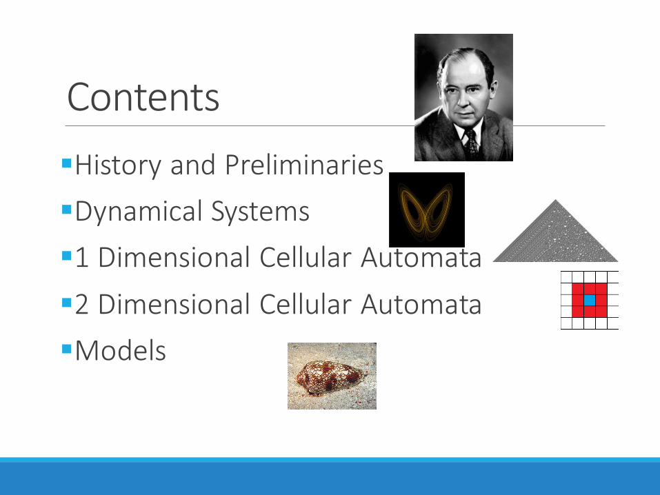
▪Self Replicating Machines
▪Biological Systems
▪Artificial Life
History: Motivations
Preliminaries: Turing Machines
▪Alan Turing (1936)
▪Minsky’s UTM : 7 head states, 4 cell states
▪Wolfram using rule 110 : 2 head states, 5 cell states
▪Wolfram: offering prize to a 2-3 UTM[1]
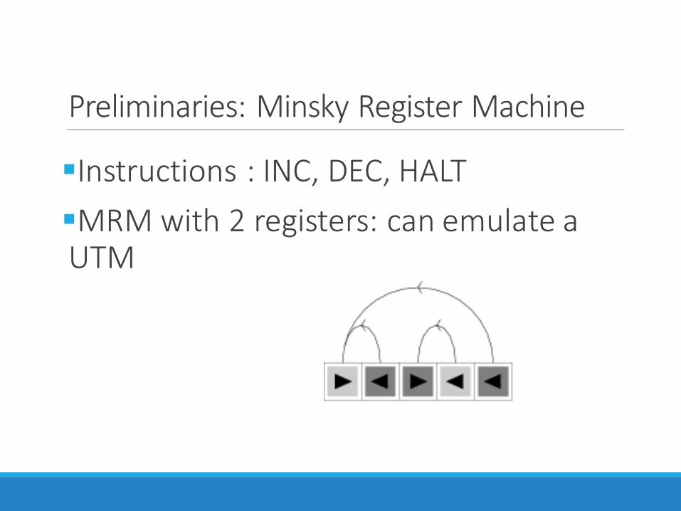
Preliminaries: Minsky Register Machine
▪Instructions : INC, DEC, HALT
▪MRM with 2 registers: can emulate a UTM
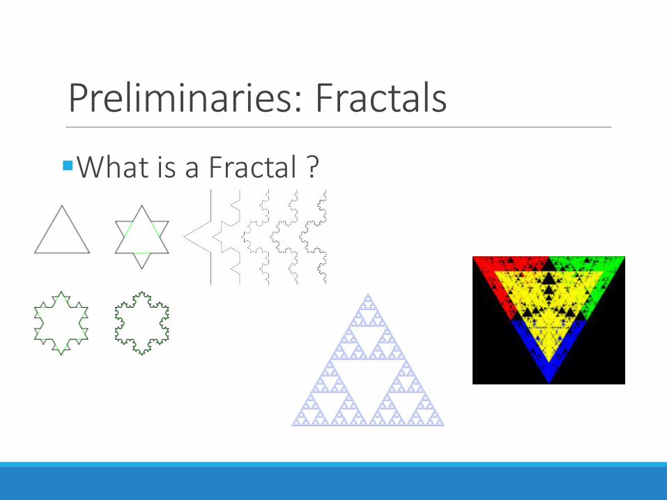
Preliminaries: Fractals
▪What is a Fractal ?
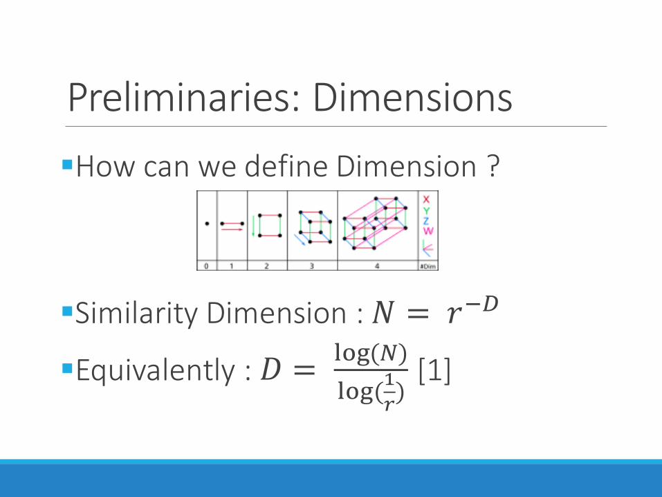
Preliminaries: Dimensions
▪How can we define Dimension ?
▪Similarity Dimension : 𝑁 = 𝑟−𝐷
▪Equivalently : [1]

Preliminaries: Dimensions
▪Fractal : Any figure with a non-integer dimension.
▪Intuitively a dimension of 1.262 (Koch Curve) shows that the figure seems to be taking space more than an ordinary line [1][2]
Preliminaries: Information
▪Claude Shannon (1948) : Being unlikely to occur, an event upon it’s occurrence exposes more “information”. (and vice-a-versa)[1]
▪Being unlikely to occur : having low probability of occurrence
Preliminaries: Information
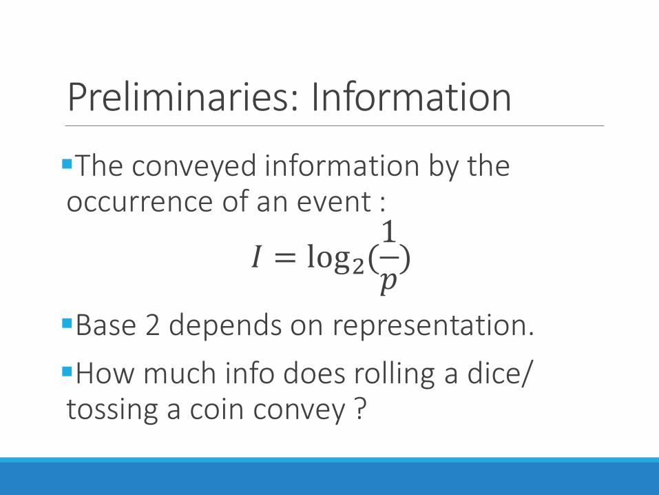
▪The conveyed information by the occurrence of an event :
▪Base 2 depends on representation.
▪How much info does rolling a dice/ tossing a coin convey ?
Preliminaries: Entropy
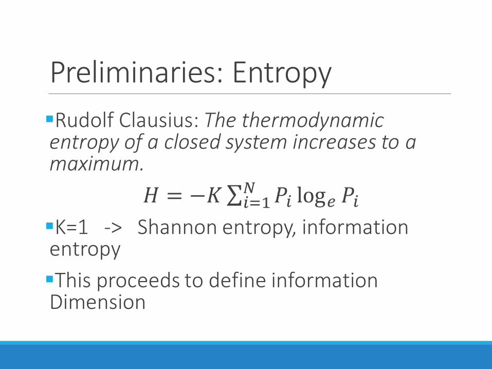
▪Rudolf Clausius: The thermodynamic entropy of a closed system increases to a maximum.
𝐻 = −𝐾σ𝑖=1𝑁 𝑃𝑖 log𝑒 𝑃𝑖
▪K=1 -> Shannon entropy, information entropy
▪This proceeds to define information Dimension
Preliminaries: Randomness
▪High Entropy : High disorder , Randomness
▪Random: unpredictable
▪More technical : an infinitely long sequence is random if it’s Shannon information (I) is infinite.
▪Quantis, the only real random number generator
▪Randomness vs pseudo-randomness
Dynamical Systems
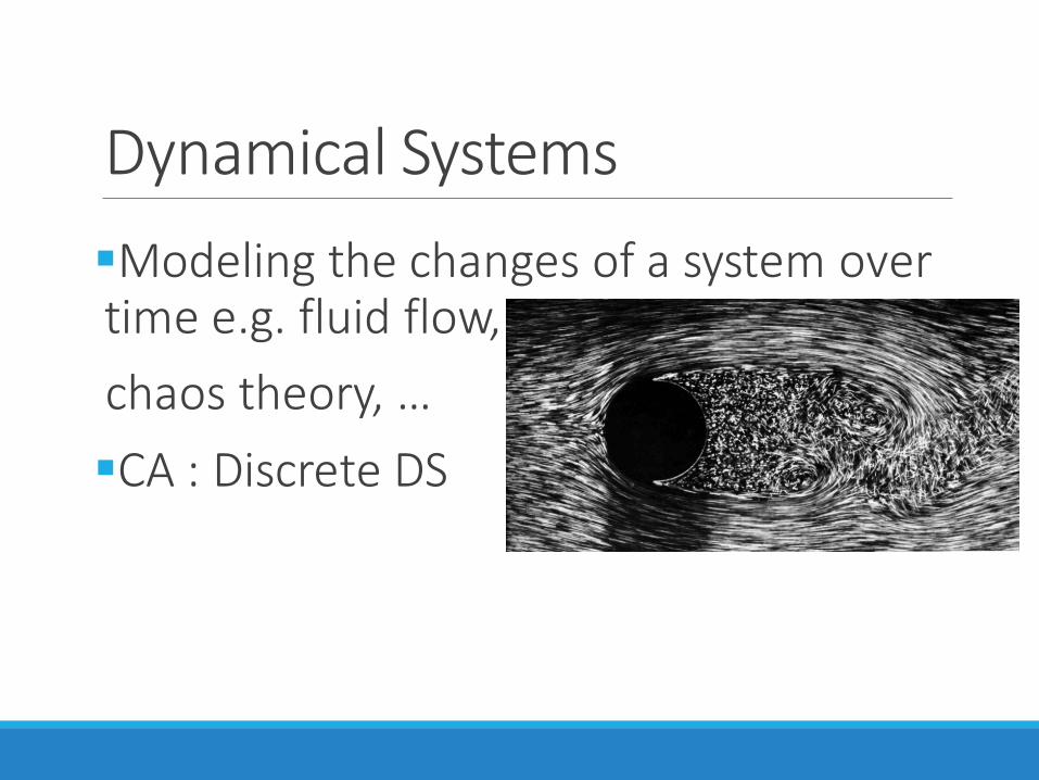
▪Modeling the changes of a system over time e.g. fluid flow,
chaos theory, …
▪CA : Discrete DS
Dynamical Systems
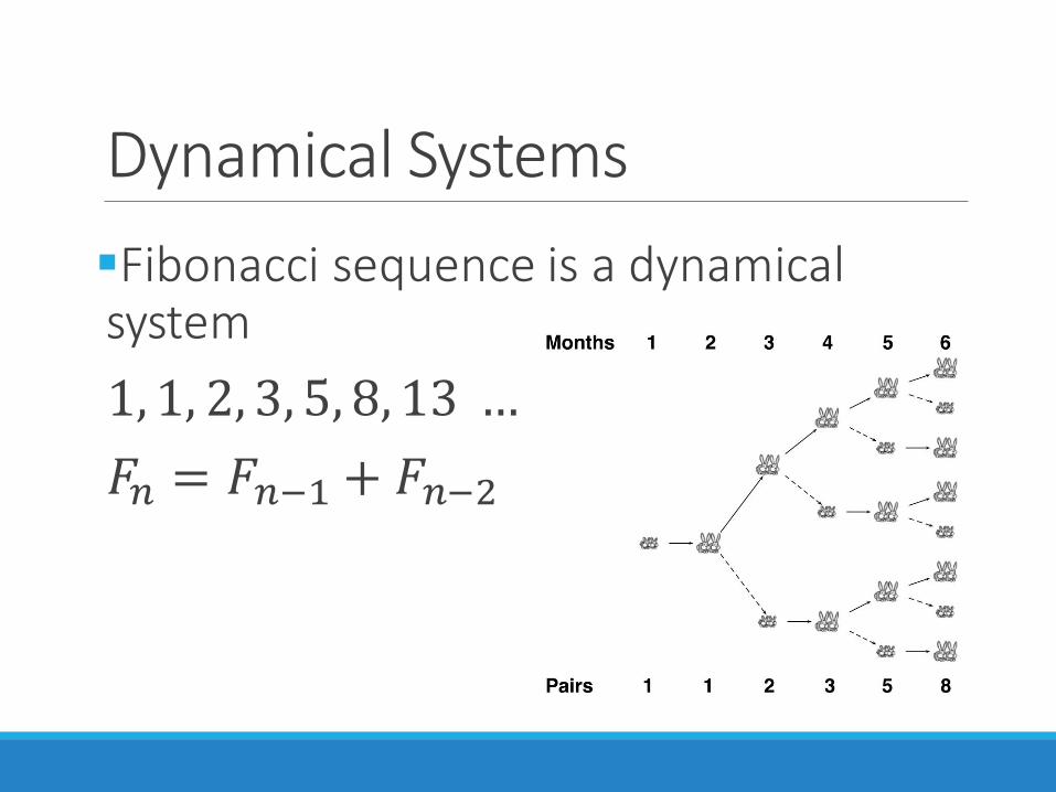
▪Fibonacci sequence is a dynamical system
1, 1, 2, 3, 5, 8, 13 …
𝐹𝑛 = 𝐹𝑛−1 + 𝐹𝑛−2
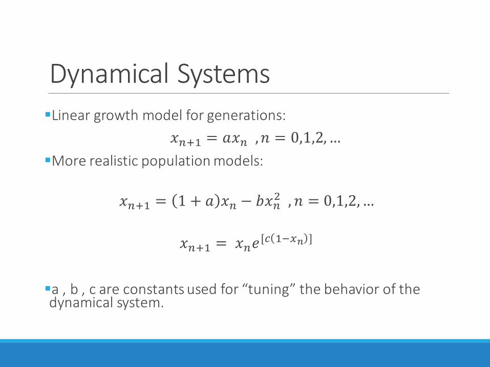
Dynamical Systems▪Linear growth model for generations:
𝑥𝑛+1 = 𝑎𝑥𝑛 , 𝑛 = 0,1,2,…
▪More realistic population models:
𝑥𝑛+1 = 1 + 𝑎 𝑥𝑛 − 𝑏𝑥𝑛2 , 𝑛 = 0,1,2,…
𝑥𝑛+1 = 𝑥𝑛𝑒[𝑐 1−𝑥𝑛 ]
▪a , b , c are constants used for “tuning” the behavior of the dynamical system.
Dynamical Systems
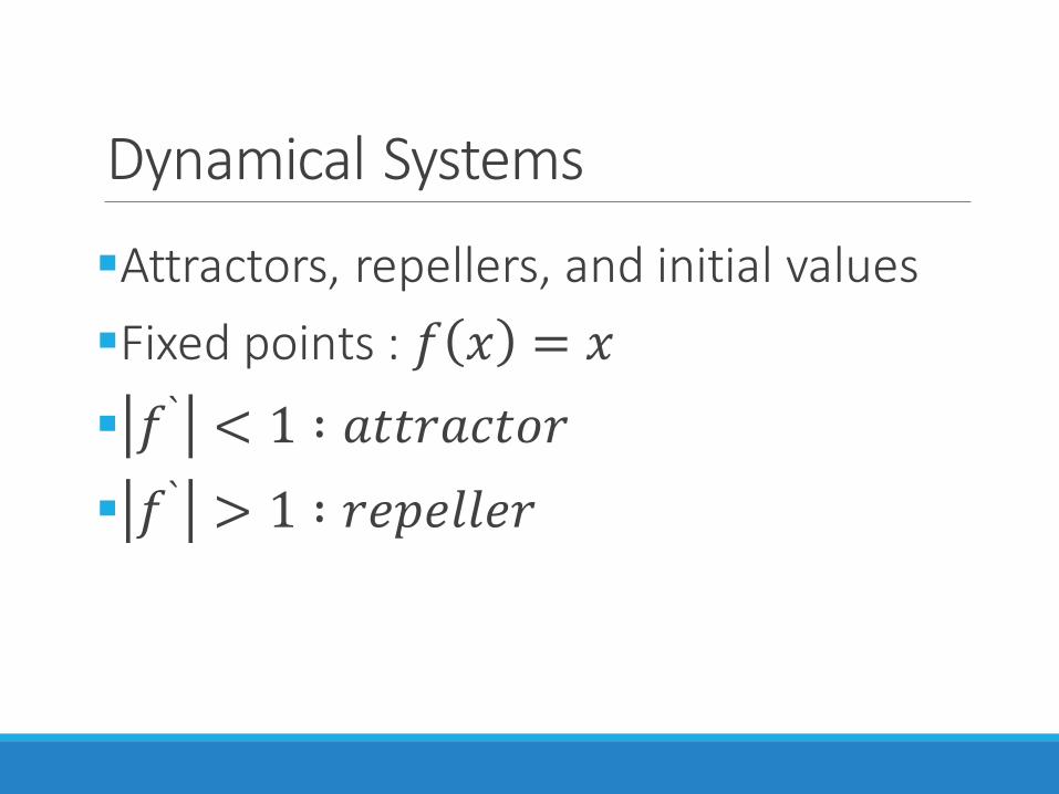
▪Attractors, repellers, and initial values
▪Fixed points : 𝑓 𝑥 = 𝑥
Dynamical Systems
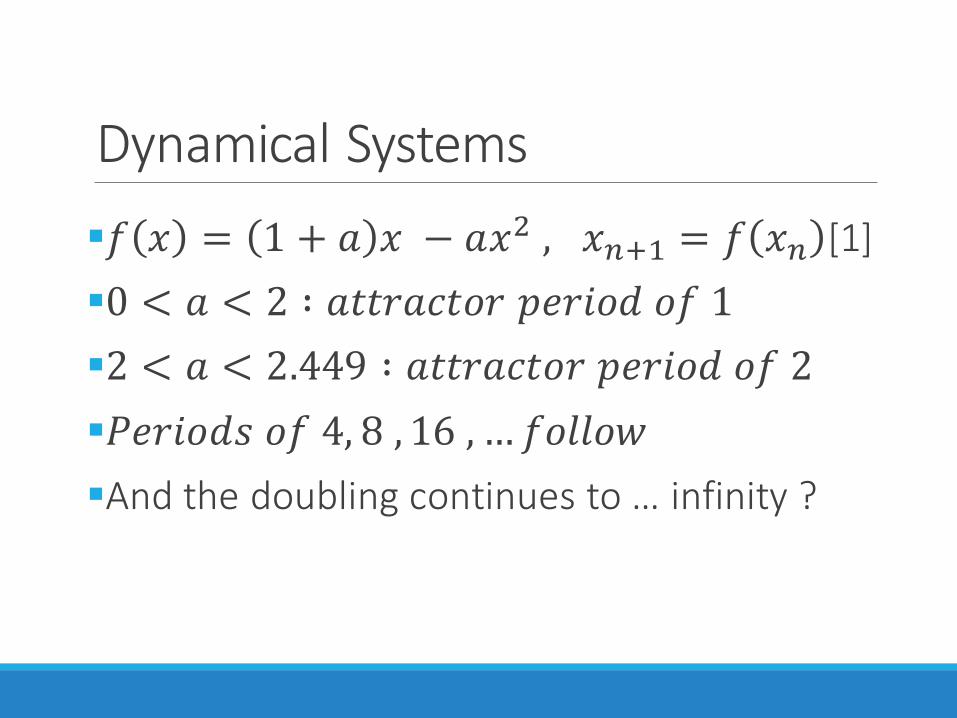
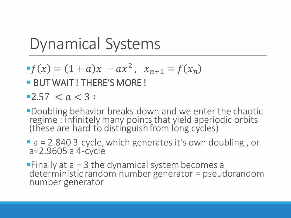
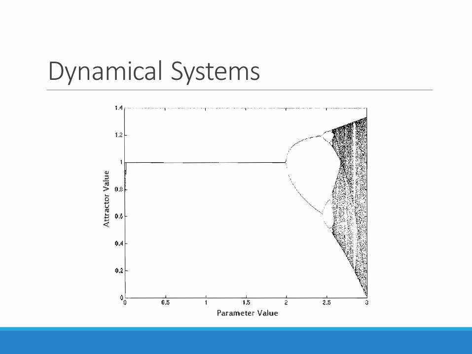
▪𝑓 𝑥 = 1 + 𝑎 𝑥 − 𝑎𝑥2 , 𝑥𝑛+1 = 𝑓 𝑥𝑛 [1]
▪0 < 𝑎 < 2 ∶ 𝑎𝑡𝑡𝑟𝑎𝑐𝑡𝑜𝑟 𝑝𝑒𝑟𝑖𝑜𝑑 𝑜𝑓 1
▪2 < 𝑎 < 2.449 ∶ 𝑎𝑡𝑡𝑟𝑎𝑐𝑡𝑜𝑟 𝑝𝑒𝑟𝑖𝑜𝑑 𝑜𝑓 2
▪𝑃𝑒𝑟𝑖𝑜𝑑𝑠 𝑜𝑓 4, 8 , 16 , … 𝑓𝑜𝑙𝑙𝑜𝑤
▪And the doubling continues to … infinity ?
Dynamical Systems
▪𝑓 𝑥 = 1+ 𝑎 𝑥 − 𝑎𝑥2 , 𝑥𝑛+1 = 𝑓 𝑥𝑛▪ BUT WAIT ! THERE’S MORE !
▪2.57 < 𝑎 < 3 ∶
▪Doubling behavior breaks down and we enter the chaotic regime : infinitely many points that yield aperiodic orbits (these are hard to distinguish from long cycles)
▪ a = 2.840 3-cycle, which generates it’s own doubling , or a=2.9605 a 4-cycle
▪Finally at a = 3 the dynamical system becomes a deterministic random number generator = pseudorandom number generator
Dynamical Systems
1D Cellular Automata: Intro
▪A lattice of cells usually square shaped , each of which can be in k different states, one of which is named quiescent
▪Dimension and size of the lattice
▪Local transition function and time steps
▪State transformation and neighbors
▪A cellular automaton : cells, transition function, set of states.

1D Cellular Automata: Example
Initial position (start state)
1D Cellular Automata: Example
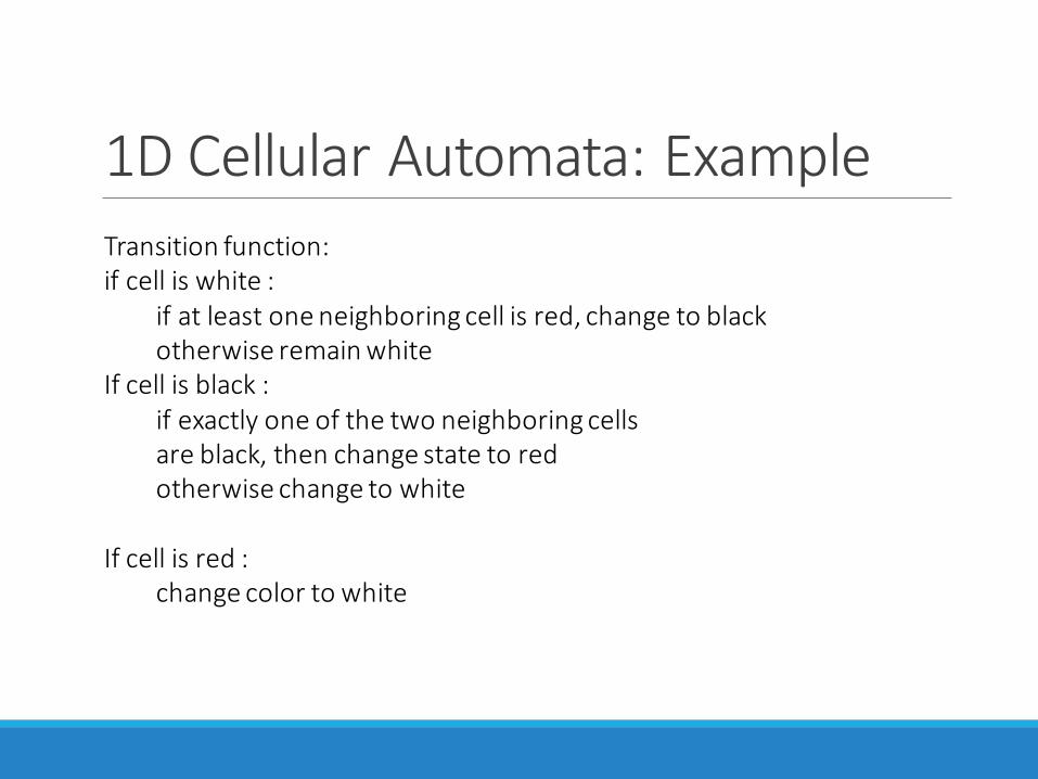
Transition function: if cell is white :
if at least one neighboring cell is red, change to blackotherwise remain white
If cell is black : if exactly one of the two neighboring cellsare black, then change state to redotherwise change to white
If cell is red : change color to white
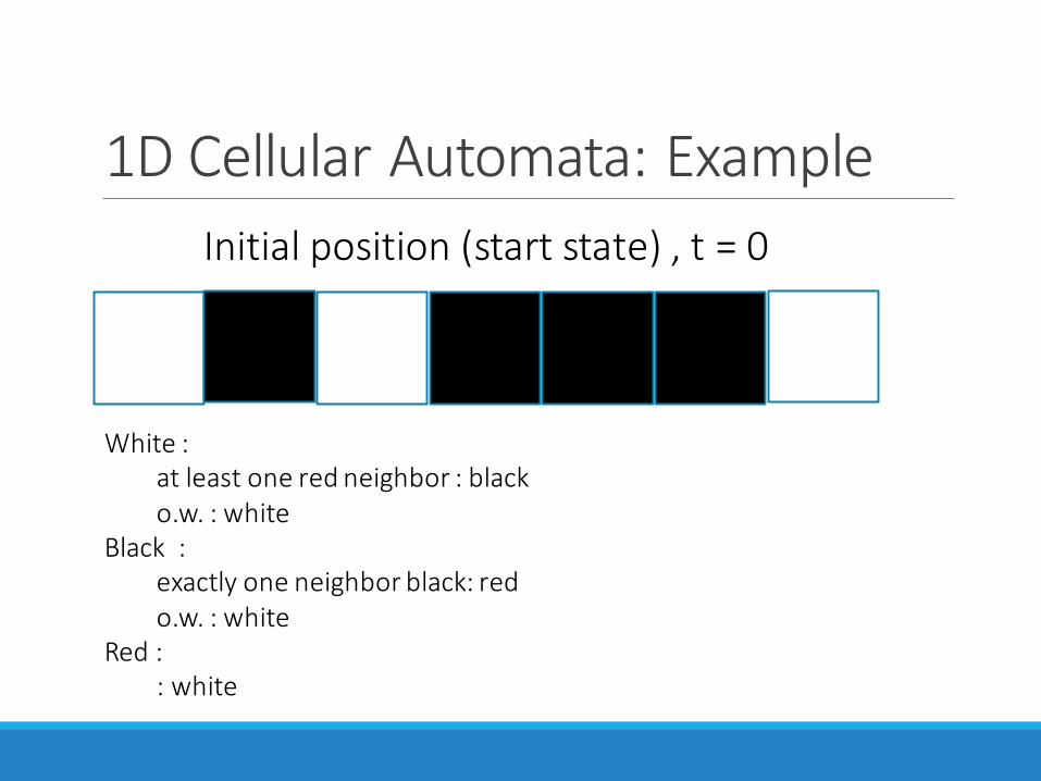
1D Cellular Automata: Example
Initial position (start state) , t = 0
White : at least one red neighbor : blacko.w. : white
Black :exactly one neighbor black: redo.w. : white
Red : : white
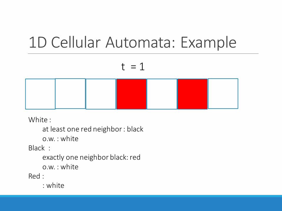
1D Cellular Automata: Example
t = 1
White : at least one red neighbor : blacko.w. : white
Black :exactly one neighbor black: redo.w. : white
Red : : white
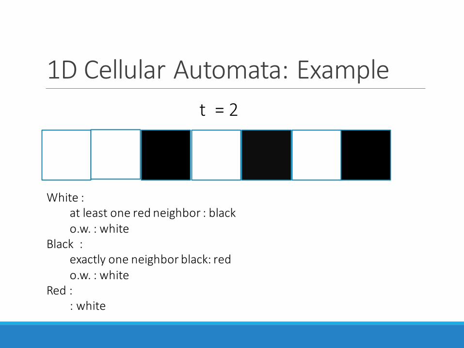
1D Cellular Automata: Example
t = 2
White : at least one red neighbor : blacko.w. : white
Black :exactly one neighbor black: redo.w. : white
Red : : white
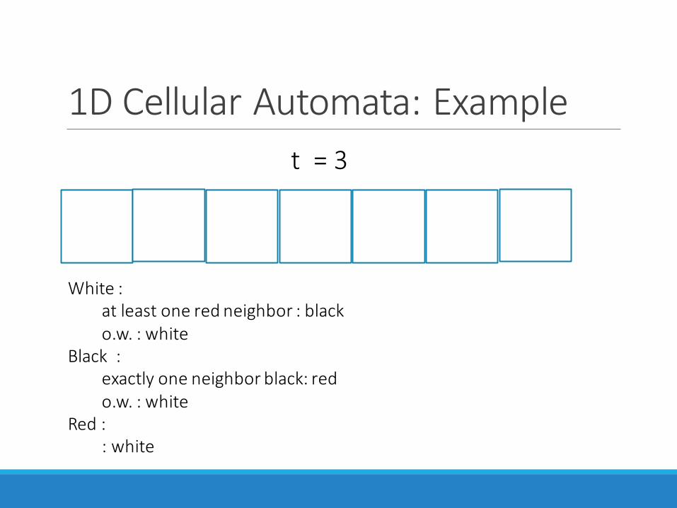
1D Cellular Automata: Example
t = 3
White : at least one red neighbor : blacko.w. : white
Black :exactly one neighbor black: redo.w. : white
Red : : white
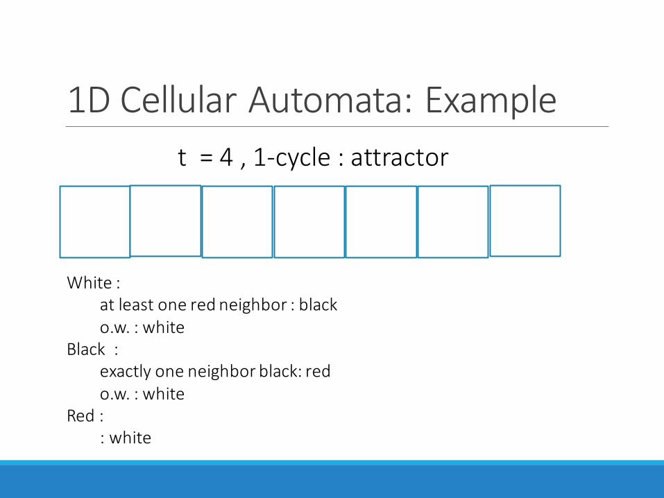
1D Cellular Automata: Example
t = 4 , 1-cycle : attractor
White : at least one red neighbor : blacko.w. : white
Black :exactly one neighbor black: redo.w. : white
Red : : white
1D Cellular Automata: Properties
▪Uniformity
▪Synchronicity
▪Locality

1D Cellular Automata: Transition Functions Formalism
▪Example :
▪𝑐𝑖 𝑡 + 1 = 𝑐𝑖 −1 𝑡 − 1 + 𝑐𝑖+1 𝑡 − 1 𝑚𝑜𝑑 2
▪Convenient way for radius neighborhood :
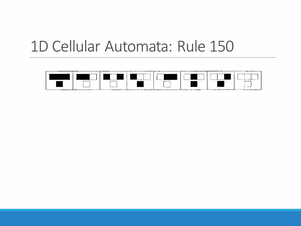
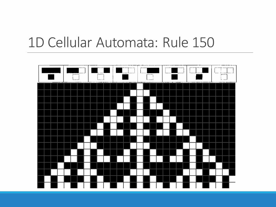
1D Cellular Automata: Rule 150
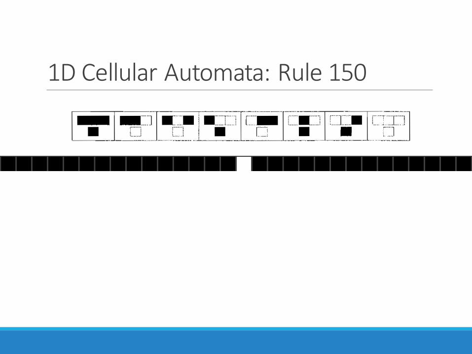
1D Cellular Automata: Rule 150
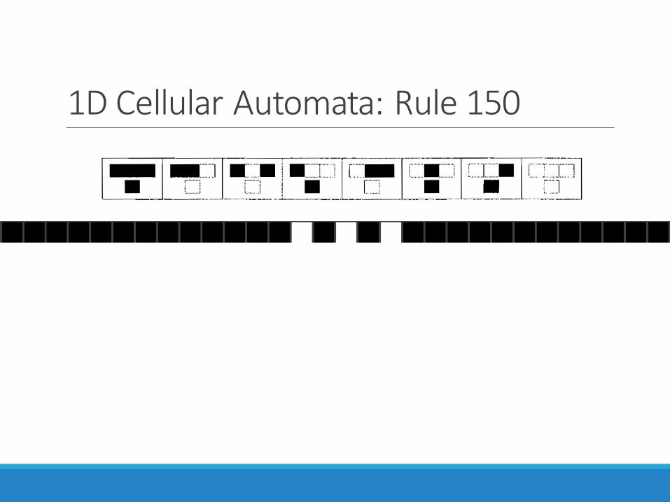
1D Cellular Automata: Rule 150
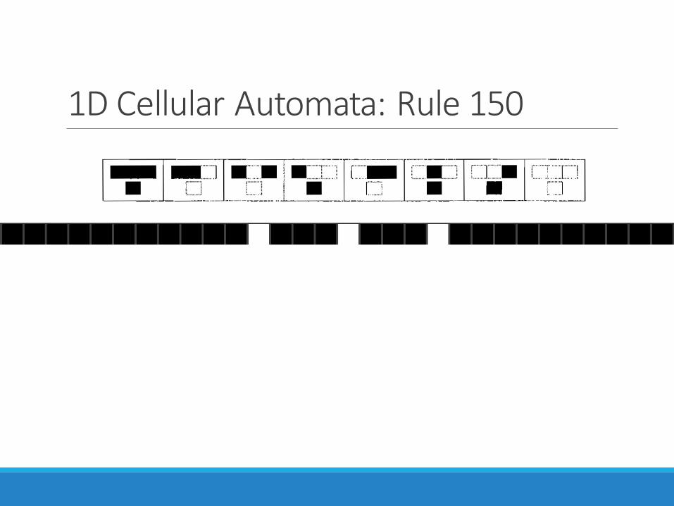
1D Cellular Automata: Rule 150
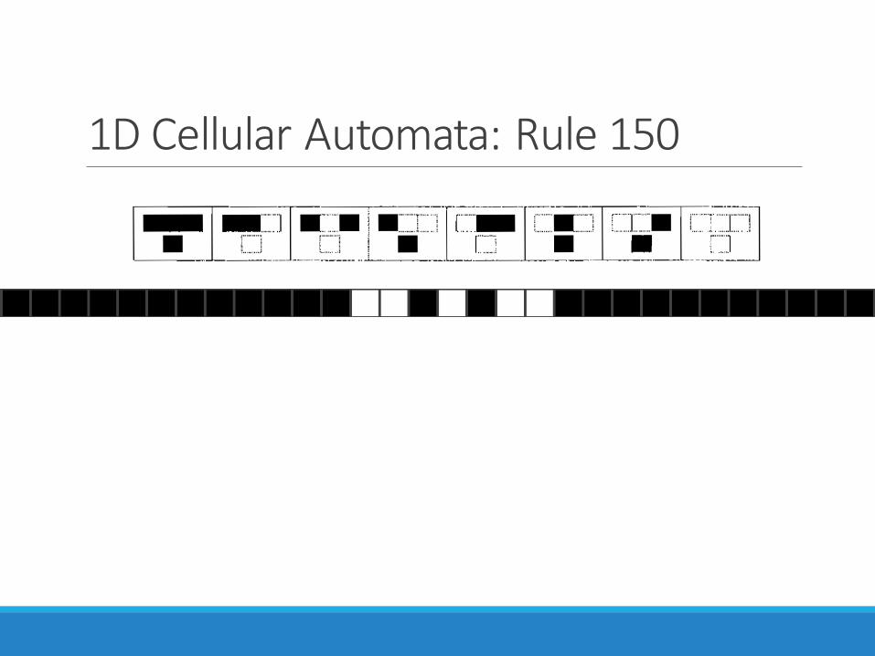
1D Cellular Automata: Rule 150

1D Cellular Automata: Rule 150
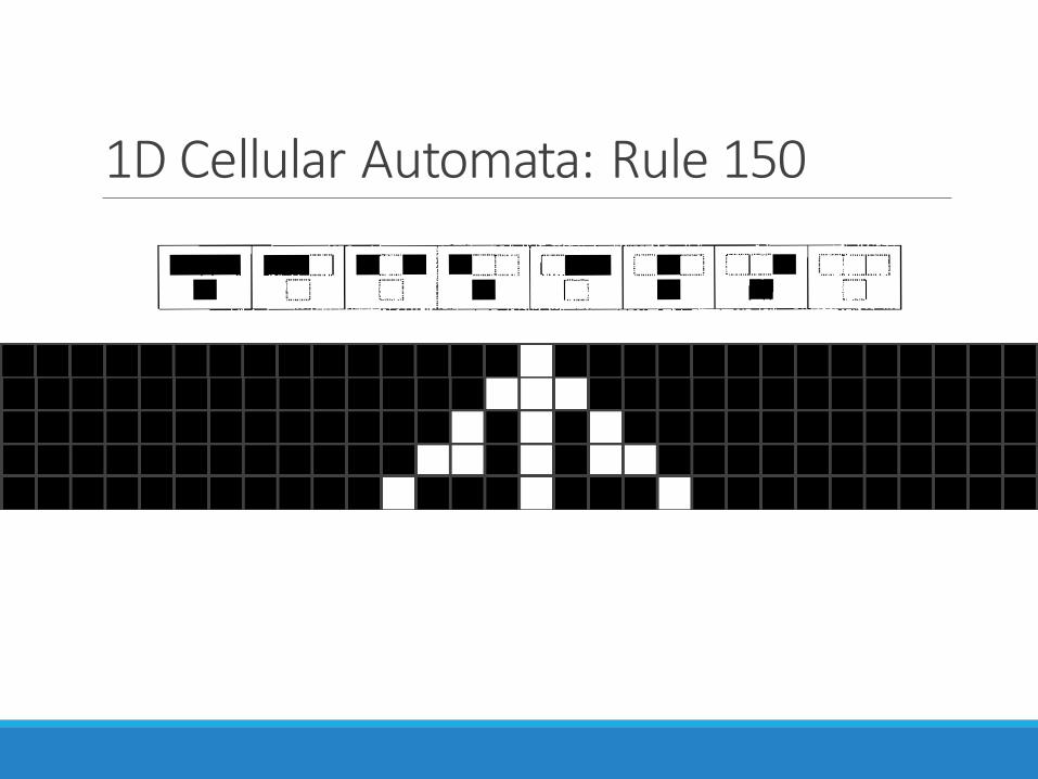
1D Cellular Automata: Rule 150
1D Cellular Automata: Rule 150
1D Cellular Automata: reversibility
▪Is cellular automata behavior reversible?
▪State compression results in low entropy
▪Only a small percentage of cellular automata are reversible
1D Cellular Automata: Classification
▪1980: Wolfram began classifying cellular automata
▪4 classes, majority of automata can be classified using these classes
1D Cellular Automata: Classification
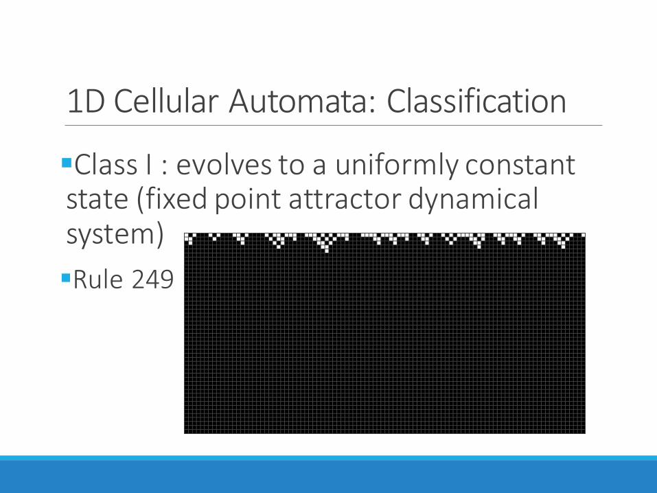
▪Class I : evolves to a uniformly constant state (fixed point attractor dynamical system)
▪Rule 249
1D Cellular Automata: Classification
▪Class II : repeats in periodic cycles.
▪Similar to these are systems of finite size
▪Can be used in digital image processing
1D Cellular Automata: Classification
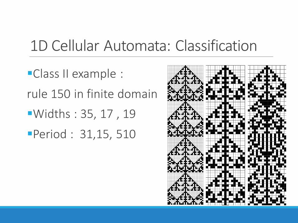
▪Class II example :
rule 150 in finite domain
▪Widths : 35, 17 , 19
▪Period : 31,15, 510
1D Cellular Automata: Classification
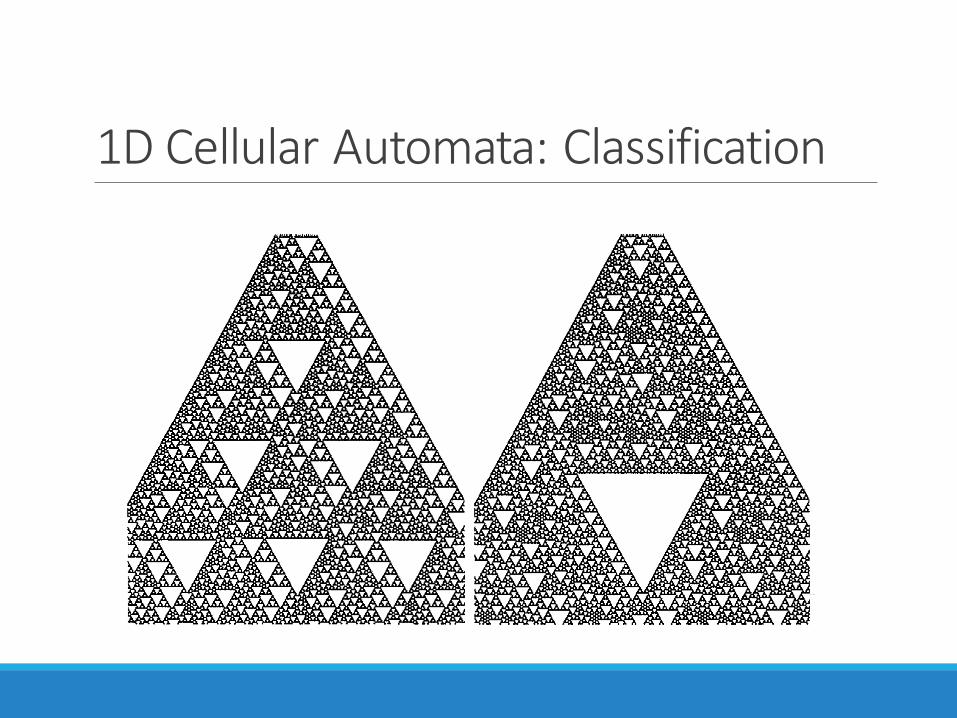
▪Class III: random behavior, typically with triangular features present
▪Analogous to chaotic dynamical systems
▪Very sensitive to initial conditions
▪Useful in study of randomness
▪Rule 126
1D Cellular Automata: Classification
1D Cellular Automata: Classification
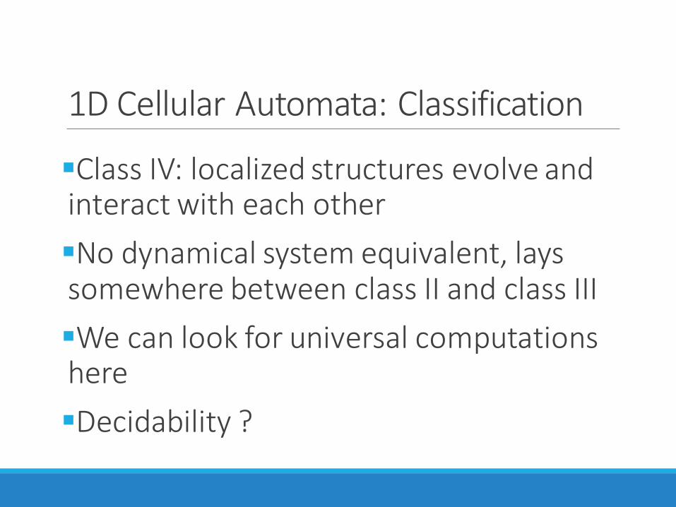
▪Class IV: localized structures evolve and interact with each other
▪No dynamical system equivalent, lays somewhere between class II and class III
▪We can look for universal computations here
▪Decidability ?
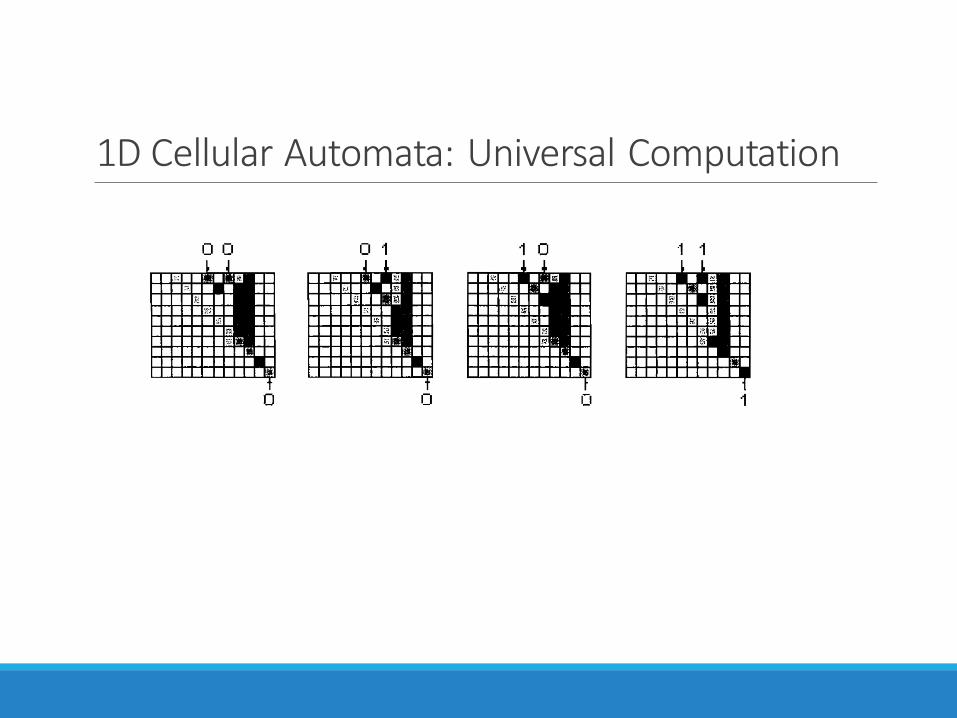
1D Cellular Automata: Universal Computation

1D Cellular Automata: Notable Problem
▪Firing Squad Problem
▪n cells : 3n -1 solution exists
▪Minimal time solution : 2n-1
▪Mazoyer : 6 state minimal time
▪No minimal time with 4 states
▪5 or 6 states ? Still open :) [1]
2D Cellular Automata: Intro
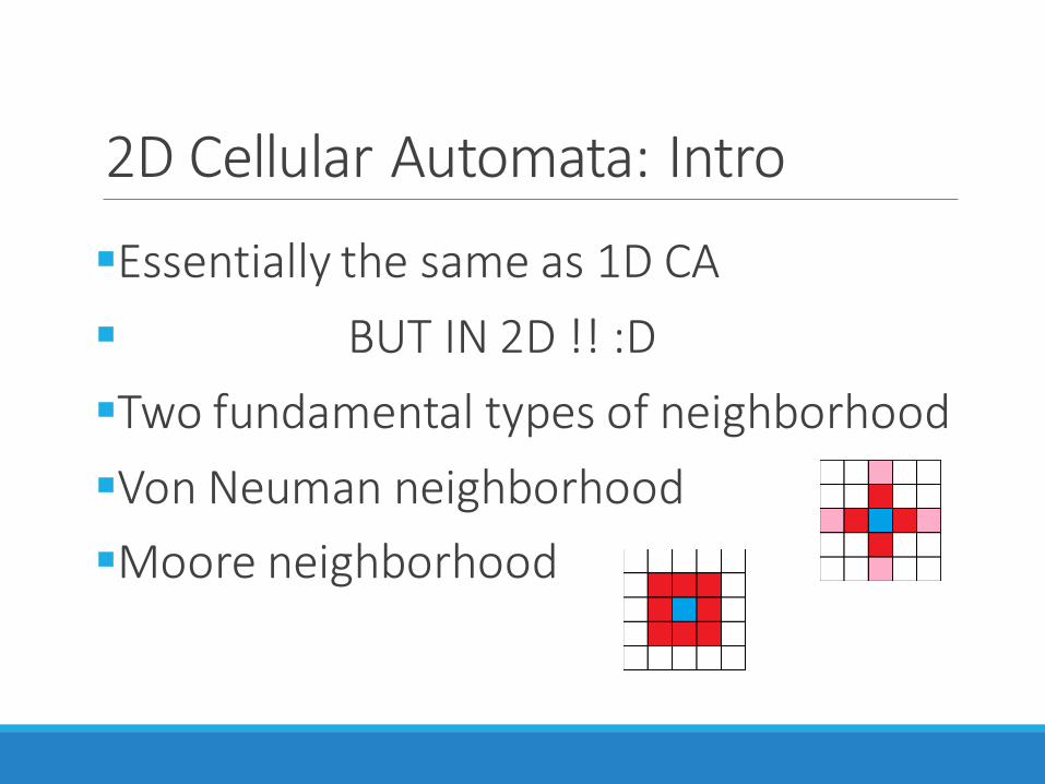
▪Essentially the same as 1D CA
▪ BUT IN 2D !! :D
▪Two fundamental types of neighborhood
▪Von Neuman neighborhood
▪Moore neighborhood
2D Cellular Automata: Game of Life
▪2 states per cell
▪A Dead cell becomes alive if exactly three neighbors are alive (eight-cell Moore neighborhood)
▪An alive cell remains alive if either 2 or three of it’s neighbors are alive
▪Many variants exist
2D Cellular Automata: Game of Life
▪Game of life is a class IV CA.
▪No other class IV CA found (except trivial variants of life)
2D Cellular Automata: Game of Life
▪$50 prize was offered to the person who could prove or disprove that …
▪… No initial position of live cells could grow unboundedly
▪ What do you think ?
2D Cellular Automata: Game of Life, Life forms
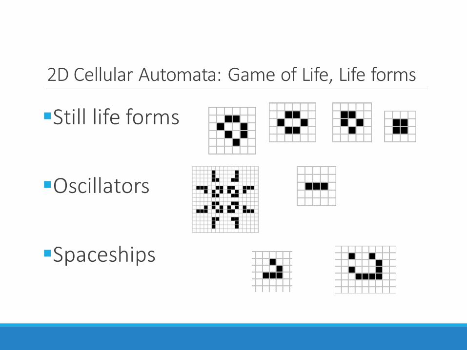
▪Still life forms
▪Oscillators
▪Spaceships
2D Cellular Automata: Game of Life, Life forms
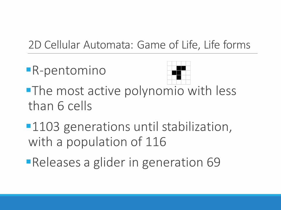
▪R-pentomino
▪The most active polynomio with less than 6 cells
▪1103 generations until stabilization, with a population of 116
▪Releases a glider in generation 69
2D Cellular Automata: Game of Life, Life forms
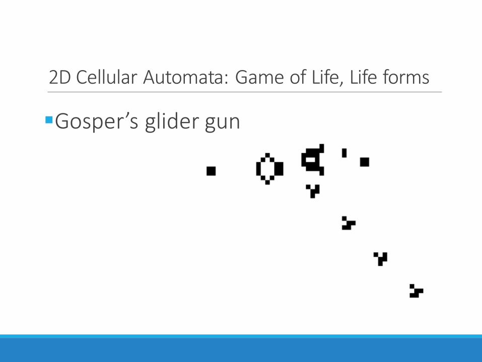
▪Gosper’s glider gun
2D Cellular Automata: Brian’s Brian
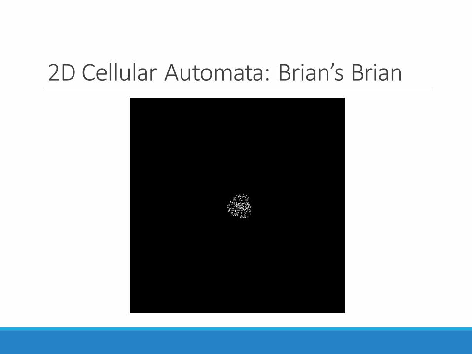
▪3 states : firing(alive), dying , off
▪A cell which is off becomes alive in the next time step if it had had two alive neighbors
▪All alive cells change into dying state and all dying cells change state to off in the next time step
2D Cellular Automata: Brian’s Brian
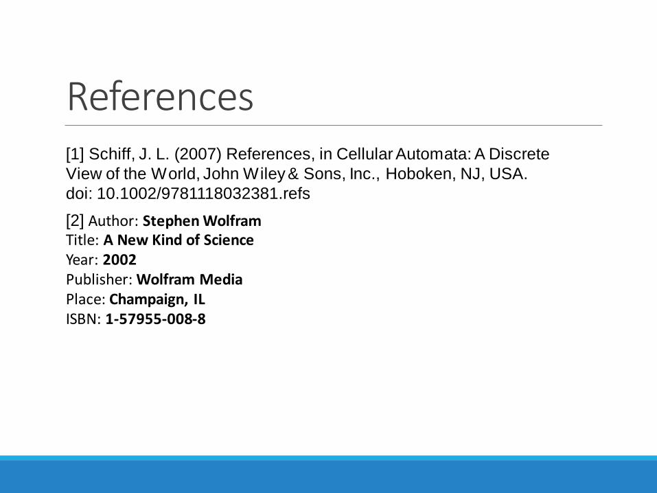
References[1] Schiff, J. L. (2007) References, in Cellular Automata: A Discrete
View of the World, John Wiley & Sons, Inc., Hoboken, NJ, USA.
doi: 10.1002/9781118032381.refs
[2] Author: Stephen WolframTitle: A New Kind of ScienceYear: 2002Publisher: Wolfram MediaPlace: Champaign, ILISBN: 1-57955-008-8