Embed Size (px)
Citation preview

Course Lecture Notes
Introduction to Causal Inferencefrom a Machine Learning Perspective
Brady Neal
December 17, 2020

Preface
Prerequisites There is one main prerequisite: basic probability. This course assumes
you’ve taken an introduction to probability course or have had equivalent experience.
Topics from statistics and machine learning will pop up in the course from time to
time, so some familiarity with those will be helpful but is not necessary. For example, if
cross-validation is a new concept to you, you can learn it relatively quickly at the point in
the book that it pops up. And we give a primer on some statistics terminology that we’ll
use in Section 2.4.
Active Reading Exercises Research shows that one of the best techniques to remember
material is to actively try to recall information that you recently learned. You will see
“active reading exercises” throughout the book to help you do this. They’ll be marked by
the Active reading exercise: heading.
Many Figures in This Book As you will see, there are a ridiculous amount of figures in
this book. This is on purpose. This is to help give you as much visual intuition as possible.
We will sometimes copy the same figures, equations, etc. that you might have seen in
preceding chapters so that we can make sure the figures are always right next to the text
that references them.
Sending Me Feedback This is a book draft, so I greatly appreciate any feedback you’re
willing to send my way. If you’re unsure whether I’ll be receptive to it or not, don’t be.
Please send any feedback to me at [email protected] with “[Causal Book]” in the
beginning of your email subject. Feedback can be at the word level, sentence level, section
level, chapter level, etc. Here’s a non-exhaustive list of useful kinds of feedback:
I Typoz.
I Some part is confusing.
I You notice your mind starts to wander, or you don’t feel motivated to read some
part.
I Some part seems like it can be cut.
I You feel strongly that some part absolutely should not be cut.
I Some parts are not connected well. Moving from one part to the next, you notice
that there isn’t a natural flow.
I A new active reading exercise you thought of.
Bibliographic Notes Although we do our best to cite relevant results, we don’t want to
disrupt the flow of the material by digging into exactly where each concept came from.
There will be complete sections of bibliographic notes in the final version of this book,
but they won’t come until after the course has finished.

Contents
Preface ii
Contents iii
1 Motivation: Why You Might Care 11.1 Simpson’s Paradox . . . . . . . . . . . . . . . . . . . . . . . . . . . . . . . . 1
1.2 Applications of Causal Inference . . . . . . . . . . . . . . . . . . . . . . . . 2
1.3 Correlation Does Not Imply Causation . . . . . . . . . . . . . . . . . . . . 3
1.3.1 Nicolas Cage and Pool Drownings . . . . . . . . . . . . . . . . . . . 3
1.3.2 Why is Association Not Causation? . . . . . . . . . . . . . . . . . . 4
1.4 Main Themes . . . . . . . . . . . . . . . . . . . . . . . . . . . . . . . . . . . 5
2 Potential Outcomes 62.1 Potential Outcomes and Individual Treatment Effects . . . . . . . . . . . . 6
2.2 The Fundamental Problem of Causal Inference . . . . . . . . . . . . . . . . 7
2.3 Getting Around the Fundamental Problem . . . . . . . . . . . . . . . . . . 8
2.3.1 Average Treatment Effects and Missing Data Interpretation . . . . 8
2.3.2 Ignorability and Exchangeability . . . . . . . . . . . . . . . . . . . 9
2.3.3 Conditional Exchangeability and Unconfoundedness . . . . . . . . 10
2.3.4 Positivity/Overlap and Extrapolation . . . . . . . . . . . . . . . . . 12
2.3.5 No interference, Consistency, and SUTVA . . . . . . . . . . . . . . 13
2.3.6 Tying It All Together . . . . . . . . . . . . . . . . . . . . . . . . . . 14
2.4 Fancy Statistics Terminology Defancified . . . . . . . . . . . . . . . . . . . 15
2.5 A Complete Example with Estimation . . . . . . . . . . . . . . . . . . . . . 16
3 The Flow of Association and Causation in Graphs 193.1 Graph Terminology . . . . . . . . . . . . . . . . . . . . . . . . . . . . . . . 19
3.2 Bayesian Networks . . . . . . . . . . . . . . . . . . . . . . . . . . . . . . . . 20
3.3 Causal Graphs . . . . . . . . . . . . . . . . . . . . . . . . . . . . . . . . . . 22
3.4 Two-Node Graphs and Graphical Building Blocks . . . . . . . . . . . . . . 23
3.5 Chains and Forks . . . . . . . . . . . . . . . . . . . . . . . . . . . . . . . . 24
3.6 Colliders and their Descendants . . . . . . . . . . . . . . . . . . . . . . . . 26
3.7 d-separation . . . . . . . . . . . . . . . . . . . . . . . . . . . . . . . . . . . 28
3.8 Flow of Association and Causation . . . . . . . . . . . . . . . . . . . . . . 30
4 Causal Models 324.1 The do-operator and Interventional Distributions . . . . . . . . . . . . . . 32
4.2 The Main Assumption: Modularity . . . . . . . . . . . . . . . . . . . . . . 34
4.3 Truncated Factorization . . . . . . . . . . . . . . . . . . . . . . . . . . . . . 35
4.3.1 Example Application and Revisiting “Association is Not Causation” 36
4.4 The Backdoor Adjustment . . . . . . . . . . . . . . . . . . . . . . . . . . . 37
4.4.1 Relation to Potential Outcomes . . . . . . . . . . . . . . . . . . . . . 39
4.5 Structural Causal Models (SCMs) . . . . . . . . . . . . . . . . . . . . . . . 40
4.5.1 Structural Equations . . . . . . . . . . . . . . . . . . . . . . . . . . 40
4.5.2 Interventions . . . . . . . . . . . . . . . . . . . . . . . . . . . . . . . 42
4.5.3 Collider Bias andWhy to Not Condition on Descendants of Treatment 43
4.6 Example Applications of the Backdoor Adjustment . . . . . . . . . . . . . 44
4.6.1 Association vs. Causation in a Toy Example . . . . . . . . . . . . . 44

4.6.2 A Complete Example with Estimation . . . . . . . . . . . . . . . . 45
4.7 Assumptions Revisited . . . . . . . . . . . . . . . . . . . . . . . . . . . . . 47
5 Randomized Experiments 495.1 Comparability and Covariate Balance . . . . . . . . . . . . . . . . . . . . . 49
5.2 Exchangeability . . . . . . . . . . . . . . . . . . . . . . . . . . . . . . . . . 50
5.3 No Backdoor Paths . . . . . . . . . . . . . . . . . . . . . . . . . . . . . . . 51
6 Nonparametric Identification 526.1 Frontdoor Adjustment . . . . . . . . . . . . . . . . . . . . . . . . . . . . . . 52
6.2 do-calculus . . . . . . . . . . . . . . . . . . . . . . . . . . . . . . . . . . . . 55
6.2.1 Application: Frontdoor Adjustment . . . . . . . . . . . . . . . . . . 57
6.3 Determining Identifiability from the Graph . . . . . . . . . . . . . . . . . . 58
7 Estimation 627.1 Preliminaries . . . . . . . . . . . . . . . . . . . . . . . . . . . . . . . . . . . 62
7.2 Conditional Outcome Modeling (COM) . . . . . . . . . . . . . . . . . . . . 63
7.3 Grouped Conditional Outcome Modeling (GCOM) . . . . . . . . . . . . . 64
7.4 Increasing Data Efficiency . . . . . . . . . . . . . . . . . . . . . . . . . . . . 65
7.4.1 TARNet . . . . . . . . . . . . . . . . . . . . . . . . . . . . . . . . . . 65
7.4.2 X-Learner . . . . . . . . . . . . . . . . . . . . . . . . . . . . . . . . . 66
7.5 Propensity Scores . . . . . . . . . . . . . . . . . . . . . . . . . . . . . . . . 67
7.6 Inverse Probability Weighting (IPW) . . . . . . . . . . . . . . . . . . . . . . 68
7.7 Doubly Robust Methods . . . . . . . . . . . . . . . . . . . . . . . . . . . . 70
7.8 Other Methods . . . . . . . . . . . . . . . . . . . . . . . . . . . . . . . . . . 70
7.9 Concluding Remarks . . . . . . . . . . . . . . . . . . . . . . . . . . . . . . 71
7.9.1 Confidence Intervals . . . . . . . . . . . . . . . . . . . . . . . . . . 71
7.9.2 Comparison to Randomized Experiments . . . . . . . . . . . . . . 72
8 Unobserved Confounding: Bounds and Sensitivity Analysis 738.1 Bounds . . . . . . . . . . . . . . . . . . . . . . . . . . . . . . . . . . . . . . 73
8.1.1 No-Assumptions Bound . . . . . . . . . . . . . . . . . . . . . . . . 74
8.1.2 Monotone Treatment Response . . . . . . . . . . . . . . . . . . . . 76
8.1.3 Monotone Treatment Selection . . . . . . . . . . . . . . . . . . . . . 78
8.1.4 Optimal Treatment Selection . . . . . . . . . . . . . . . . . . . . . . 79
8.2 Sensitivity Analysis . . . . . . . . . . . . . . . . . . . . . . . . . . . . . . . 82
8.2.1 Sensitivity Basics in Linear Setting . . . . . . . . . . . . . . . . . . . 82
8.2.2 More General Settings . . . . . . . . . . . . . . . . . . . . . . . . . 85
9 Instrumental Variables 869.1 What is an Instrument? . . . . . . . . . . . . . . . . . . . . . . . . . . . . . 86
9.2 No Nonparametric Identification of the ATE . . . . . . . . . . . . . . . . . 87
9.3 Warm-Up: Binary Linear Setting . . . . . . . . . . . . . . . . . . . . . . . . 87
9.4 Continuous Linear Setting . . . . . . . . . . . . . . . . . . . . . . . . . . . 88
9.5 Nonparametric Identification of Local ATE . . . . . . . . . . . . . . . . . . 90
9.5.1 New Potential Notation with Instruments . . . . . . . . . . . . . . 90
9.5.2 Principal Stratification . . . . . . . . . . . . . . . . . . . . . . . . . 90
9.5.3 Local ATE . . . . . . . . . . . . . . . . . . . . . . . . . . . . . . . . 91
9.6 More General Settings for ATE Identification . . . . . . . . . . . . . . . . . 94
10 Difference in Differences 9510.1 Preliminaries . . . . . . . . . . . . . . . . . . . . . . . . . . . . . . . . . . . 95

10.2 Introducing Time . . . . . . . . . . . . . . . . . . . . . . . . . . . . . . . . 96
10.3 Identification . . . . . . . . . . . . . . . . . . . . . . . . . . . . . . . . . . . 96
10.3.1 Assumptions . . . . . . . . . . . . . . . . . . . . . . . . . . . . . . . 96
10.3.2 Main Result and Proof . . . . . . . . . . . . . . . . . . . . . . . . . 97
10.4 Major Problems . . . . . . . . . . . . . . . . . . . . . . . . . . . . . . . . . 98
11 Causal Discovery from Observational Data 10011.1 Independence-Based Causal Discovery . . . . . . . . . . . . . . . . . . . . 100
11.1.1 Assumptions and Theorem . . . . . . . . . . . . . . . . . . . . . . . 100
11.1.2 The PC Algorithm . . . . . . . . . . . . . . . . . . . . . . . . . . . . 102
11.1.3 Can We Get Any Better Identification? . . . . . . . . . . . . . . . . 104
11.2 Semi-Parametric Causal Discovery . . . . . . . . . . . . . . . . . . . . . . . 104
11.2.1 No Identifiability Without Parametric Assumptions . . . . . . . . . 105
11.2.2 Linear Non-Gaussian Noise . . . . . . . . . . . . . . . . . . . . . . 105
11.2.3 Nonlinear Models . . . . . . . . . . . . . . . . . . . . . . . . . . . . 108
11.3 Further Resources . . . . . . . . . . . . . . . . . . . . . . . . . . . . . . . . 109
12 Causal Discovery from Interventional Data 11012.1 Structural Interventions . . . . . . . . . . . . . . . . . . . . . . . . . . . . . 110
12.1.1 Single-Node Interventions . . . . . . . . . . . . . . . . . . . . . . . 110
12.1.2 Multi-Node Interventions . . . . . . . . . . . . . . . . . . . . . . . 110
12.2 Parametric Interventions . . . . . . . . . . . . . . . . . . . . . . . . . . . . 110
12.2.1 Coming Soon . . . . . . . . . . . . . . . . . . . . . . . . . . . . . . 110
12.3 Interventional Markov Equivalence . . . . . . . . . . . . . . . . . . . . . . 110
12.3.1 Coming Soon . . . . . . . . . . . . . . . . . . . . . . . . . . . . . . 110
12.4 Miscellaneous Other Settings . . . . . . . . . . . . . . . . . . . . . . . . . . 110
12.4.1 Coming Soon . . . . . . . . . . . . . . . . . . . . . . . . . . . . . . 110
13 Transfer Learning and Transportability 11113.1 Causal Insights for Transfer Learning . . . . . . . . . . . . . . . . . . . . . 111
13.1.1 Coming Soon . . . . . . . . . . . . . . . . . . . . . . . . . . . . . . 111
13.2 Transportability of Causal Effects Across Populations . . . . . . . . . . . . 111
13.2.1 Coming Soon . . . . . . . . . . . . . . . . . . . . . . . . . . . . . . 111
14 Counterfactuals and Mediation 11214.1 Counterfactuals Basics . . . . . . . . . . . . . . . . . . . . . . . . . . . . . 112
14.1.1 Coming Soon . . . . . . . . . . . . . . . . . . . . . . . . . . . . . . 112
14.2 Important Application: Mediation . . . . . . . . . . . . . . . . . . . . . . . 112
14.2.1 Coming Soon . . . . . . . . . . . . . . . . . . . . . . . . . . . . . . 112
Appendix 113
A Proofs 114A.1 Proof of Equation 6.1 from Section 6.1 . . . . . . . . . . . . . . . . . . . . . 114
A.2 Proof of Propensity Score Theorem (7.1) . . . . . . . . . . . . . . . . . . . . 114
A.3 Proof of IPW Estimand (7.18) . . . . . . . . . . . . . . . . . . . . . . . . . . 115
Bibliography 117
Alphabetical Index 123

List of Figures
1.1 Causal structure for when to prefer treatment B for COVID-27 . . . . . . . . . 2
1.2 Causal structure for when to prefer treatment A for COVID-27 . . . . . . . . . 2
1.3 Number of Nicolas Cage movies correlates with number of pool drownings . 3
1.4 Causal structure with getting lit as a confounder . . . . . . . . . . . . . . . . . 4
2.2 Causal structure for ignorable treatment assignment mechanism . . . . . . . . 9
2.1 Causal structure of - confounding the effect of ) on . . . . . . . . . . . . . . 9
2.3 Causal structure of confounding through - . . . . . . . . . . . . . . . . . . . . 11
2.4 Causal structure for conditional exchangeability given - . . . . . . . . . . . . 11
2.5 The Identification-Estimation Flowchart . . . . . . . . . . . . . . . . . . . . . . 16
3.3 Directed graph . . . . . . . . . . . . . . . . . . . . . . . . . . . . . . . . . . . . 19
3.1 Terminology machine gun . . . . . . . . . . . . . . . . . . . . . . . . . . . . . . 19
3.2 Undirected graph . . . . . . . . . . . . . . . . . . . . . . . . . . . . . . . . . . . 19
3.4 Directed graph with cycle . . . . . . . . . . . . . . . . . . . . . . . . . . . . . . 19
3.5 Directed graph with immorality . . . . . . . . . . . . . . . . . . . . . . . . . . 20
3.6 Four node DAG where -4 locally depends on only -3 . . . . . . . . . . . . . . 20
3.7 Four node DAG with many independencies . . . . . . . . . . . . . . . . . . . . 21
3.8 Two connected node DAG . . . . . . . . . . . . . . . . . . . . . . . . . . . . . . 22
3.9 Basic graph building blocks . . . . . . . . . . . . . . . . . . . . . . . . . . . . . 24
3.11 Two connected node DAG . . . . . . . . . . . . . . . . . . . . . . . . . . . . . . 24
3.12 Chain with association . . . . . . . . . . . . . . . . . . . . . . . . . . . . . . . . 24
3.10 Two unconnected node DAG . . . . . . . . . . . . . . . . . . . . . . . . . . . . 24
3.13 Fork with association . . . . . . . . . . . . . . . . . . . . . . . . . . . . . . . . . 25
3.14 Chain with blocked association . . . . . . . . . . . . . . . . . . . . . . . . . . . 25
3.15 Fork with blocked association . . . . . . . . . . . . . . . . . . . . . . . . . . . . 25
3.16 Immorality with association blocked by collider . . . . . . . . . . . . . . . . . 26
3.17 Immorality with association unblocked . . . . . . . . . . . . . . . . . . . . . . 26
3.18 Good-looking men are jerks example . . . . . . . . . . . . . . . . . . . . . . . . 27
3.19 Graphs for d-separation exercise . . . . . . . . . . . . . . . . . . . . . . . . . . 30
3.20Causal association and confounding association . . . . . . . . . . . . . . . . . 30
3.21 Assumptions flowchart from statistical independencies to causal dependencies 31
4.1 The Identification-Estimation Flowchart (extended) . . . . . . . . . . . . . . . 32
4.2 Illustration of the difference between conditioning and intervening . . . . . . 33
4.3 Causal mechanism . . . . . . . . . . . . . . . . . . . . . . . . . . . . . . . . . . 34
4.4 Intervention as edge deletion in causal graphs . . . . . . . . . . . . . . . . . . 35
4.5 Causal structure for application of truncated factorization . . . . . . . . . . . . 36
4.6 Manipulated graph for three nodes . . . . . . . . . . . . . . . . . . . . . . . . . 37
4.7 Graph for structural equation . . . . . . . . . . . . . . . . . . . . . . . . . . . . 40
4.8 Causal graph for several structural equations . . . . . . . . . . . . . . . . . . . 41
4.9 Causal structure before simple intervention . . . . . . . . . . . . . . . . . . . . 42
4.10 Causal structure after simple intervention . . . . . . . . . . . . . . . . . . . . . 42
4.11 Causal graph for completely blocking causal flow . . . . . . . . . . . . . . . . 43
4.12 Causal graph for partially blocking causal flow . . . . . . . . . . . . . . . . . . 43
4.13 Causal graph where a conditioned collider induces bias . . . . . . . . . . . . . 43
4.14 Causal graph where child of a mediator is conditioned on . . . . . . . . . . . . 44

4.15 Magnified causal graph where child of a mediator is conditioned on . . . . . . 44
4.16 Causal graph for M-bias . . . . . . . . . . . . . . . . . . . . . . . . . . . . . . . 44
4.17 Causal graph for toy example . . . . . . . . . . . . . . . . . . . . . . . . . . . . 45
4.18 Causal graph for blood pressure example with collider . . . . . . . . . . . . . 46
4.19 Causal graph for M-bias with unobserved variables . . . . . . . . . . . . . . . 47
5.1 Causal structure of confounding through - . . . . . . . . . . . . . . . . . . . . 51
5.2 Causal structure when we randomize treatment . . . . . . . . . . . . . . . . . 51
6.1 Causal graph for frontdoor criterion . . . . . . . . . . . . . . . . . . . . . . . . 52
6.2 Illustration of focusing analysis to a mediator . . . . . . . . . . . . . . . . . . . 52
6.3 Illustration of steps of frontdoor adjustment . . . . . . . . . . . . . . . . . . . . 52
6.5 Equationtown . . . . . . . . . . . . . . . . . . . . . . . . . . . . . . . . . . . . . 53
6.4 Causal graph for frontdoor criterion . . . . . . . . . . . . . . . . . . . . . . . . 53
6.6 Causal graph for frontdoor criterion . . . . . . . . . . . . . . . . . . . . . . . . 54
6.7 Causal graph for frontdoor criterion . . . . . . . . . . . . . . . . . . . . . . . . 57
6.10 Causal graph for frontdoor criterion . . . . . . . . . . . . . . . . . . . . . . . . 58
6.8 Causal graph for frontdoor with, − ) edge removed . . . . . . . . . . . . . . 58
6.9 Causal graph for frontdoor with ) −" edge removed . . . . . . . . . . . . . . 58
6.11 Graph where blocking one backdoor path unblocks another . . . . . . . . . . 59
6.12 Example graph that satisfies the unconfounded children criterion . . . . . . . 60
6.13 Graphs for the questions about the unconfounded children criterion . . . . . . 61
7.1 The Identification-Estimation Flowchart . . . . . . . . . . . . . . . . . . . . . . 63
7.2 Different neural networks for different kinds of estimators . . . . . . . . . . . . 66
7.3 Simple graph where, satisfies the backdoor criterion . . . . . . . . . . . . . 68
7.5 Simple graph where, confounds the effect of ) on . . . . . . . . . . . . . . . 68
7.6 Effective graph for pseudo-population that we get by reweighting the data
generated according to the graph in Figure 7.5 using inverse probabilityweighting. 68
7.4 Graphical proof of propensity score theorem . . . . . . . . . . . . . . . . . . . 68
8.1 Unobserved confounding graph . . . . . . . . . . . . . . . . . . . . . . . . . . 73
8.2 Simple unobserved confounding graph . . . . . . . . . . . . . . . . . . . . . . 82
8.3 Simple unobserved confounding graph . . . . . . . . . . . . . . . . . . . . . . 82
8.4 Simple unobserved confounding graph . . . . . . . . . . . . . . . . . . . . . . 84
8.5 Unobserved confounding sensitivity contour plots . . . . . . . . . . . . . . . . 84
9.1 Instrumental variable graph . . . . . . . . . . . . . . . . . . . . . . . . . . . . . 86
9.2 Instrumental variable graph . . . . . . . . . . . . . . . . . . . . . . . . . . . . . 87
9.3 Instrumental variable graph . . . . . . . . . . . . . . . . . . . . . . . . . . . . . 88
9.4 Instrumental variable graph . . . . . . . . . . . . . . . . . . . . . . . . . . . . . 89
9.5 Instrumental variable graph . . . . . . . . . . . . . . . . . . . . . . . . . . . . . 89
9.6 Causal graph for the compliers and defiers . . . . . . . . . . . . . . . . . . . . 91
9.7 Causal graph for the always-takers and never taker . . . . . . . . . . . . . . . 91
11.1 Faithfulness counterexample graph. . . . . . . . . . . . . . . . . . . . . . . . . 100
11.3 Immorality Markov equivalence class . . . . . . . . . . . . . . . . . . . . . . . 101
11.2 Three Markov equivalent graphs . . . . . . . . . . . . . . . . . . . . . . . . . . 101
11.5 Complete graph. . . . . . . . . . . . . . . . . . . . . . . . . . . . . . . . . . . . 102
11.6 True graph for PC example. . . . . . . . . . . . . . . . . . . . . . . . . . . . . . 102
11.4 Chain/fork skeleton. . . . . . . . . . . . . . . . . . . . . . . . . . . . . . . . . . 102

11.8 Graph from PC after we’ve oriented the immoralities. . . . . . . . . . . . . . . 103
11.9 Graph from PC after we’ve oriented edges that would form immoralities if
they were oriented in the other (incorrect) direction. . . . . . . . . . . . . . . . 103
11.7 Illustration of the process of step 1 of PC, where we start with the complete
graph (left) and remove edges until we’ve identified the skeleton of the graph
(right), given that the true graph is the one in Figure 11.6. . . . . . . . . . . . . 103
11.10Linear fits of linear non-Gaussian data . . . . . . . . . . . . . . . . . . . . . . . 108
11.11 Residuals of linear models fit to linear non-Gaussian data . . . . . . . . . . . . 108
A.1 Causal graph for frontdoor criterion . . . . . . . . . . . . . . . . . . . . . . . . 114
List of Tables
1.1 Simpson’s paradox in COVID-27 data . . . . . . . . . . . . . . . . . . . . . . . 1
2.1 Causal Inference as Missing Data Problem . . . . . . . . . . . . . . . . . . . . . 9
3.1 Exponential number of parameters for modeling factors . . . . . . . . . . . . . 20
Listings
2.1 Python code for estimating the ATE . . . . . . . . . . . . . . . . . . . . . . 17
2.2 Python code for estimating the ATE using the coefficient of linear regression 17
4.1 Python code for estimating the ATE, without adjusting for the collider . . 46

1A key ingredient necessary to find Simp-
son’s paradox is the non-uniformity ofallocation of people to the groups. 1400of the 1500 people who received treatment
A had mild condition, whereas 500 of
the 550 people who received treatment
B had severe condition. Because people
with mild condition are less likely to die,
this means that the total mortality rate
for those with treatment A is lower than
what it would have been if mild and severe
conditions were equally split among them.
The opposite bias is true for treatment B.
Motivation: Why YouMight Care 11.1 Simpson’s Paradox . . . . . 11.2 Applications of Causal Infer-
ence . . . . . . . . . . . . . . 21.3 Correlation Does Not Imply
Causation . . . . . . . . . . 3Nicolas Cage and PoolDrownings . . . . . . . . . . 3
Why is Association Not Cau-sation? . . . . . . . . . . . . 4
1.4 Main Themes . . . . . . . . . 5
1.1 Simpson’s Paradox
Consider a purely hypothetical futurewhere there is a newdisease known
as COVID-27 that is prevalent in the human population. In this purely
hypothetical future, there are two treatments that have been developed:
treatment A and treatment B. Treatment B is more scarce than treatment
A, so the split of those currently receiving treatment A vs. treatment
B is roughly 73%/27%. You are in charge of choosing which treatment
your country will exclusively use, in a country that only cares about
minimizing loss of life.
You have data on the percentage of people who die from COVID-27,
given the treatment they were assigned and given their condition at the
time treatment was decided. Their condition is a binary variable: either
mild or severe. In this data, 16% of those who receive A die, whereas
19% of those who receive B die. However, when we examine the people
with mild condition separately from the people with severe condition,
the numbers reverse order. In the mild subpopulation, 15% of those who
receive A die, whereas 10% of those who receive B die. In the severe
subpopulation, 30% of those who receive A die, whereas 20% of those
who receive B die. We depict these percentages and the corresponding
counts in Table 1.1.
ConditionMild Severe Total
Treatment
A
15%
(210/1400)
30%
(30/100)
16%(240/1500)
B
10%(5/50)
20%(100/500)
19%
(105/550)
Table 1.1: Simpson’s paradox in COVID-27
data. The percentages denote themortality
rates in each of the groups. Lower is better.
The numbers in parentheses are the corre-
sponding counts. This apparent paradox
stems from the interpretation that treat-
ment A looks better when examining the
whole population, but treatment B looks
better in all subpopulations.
The apparent paradox stems from the fact that, in Table 1.1, the “Total”
column could be interpreted to mean that we should prefer treatment
A, whereas the “Mild” and “Severe” columns could both be interpreted
to mean that we should prefer treatment B.1In fact, the answer is that if
we know someone’s condition, we should give them treatment B, and if
we do not know their condition, we should give them treatment A. Just
kidding... that doesn’t make any sense. So really, what treatment should
you choose for your country?
Either treatment A or treatment B could be the right answer, depending
on the causal structure of the data. In other words, causality is essential to
solve Simpson’s paradox. For now, wewill just give the intuition for when
you should prefer treatment A vs. when you should prefer treatment B,
but it will be made more formal in Chapter 4.

1 Motivation: Why You Might Care 2
2 ) refers to the prescription of the treat-
ment, rather than the subsequent recep-
tion of the treatment.
Scenario 1 If the condition � is a cause of the treatment ) (Figure
1.1), treatment B is more effective at reducing mortality .. An example
scenario is where doctors decide to give treatment A to most people
who have mild conditions. And they save the more expensive and more
limited treatment B for people with severe conditions. Because having
severe condition causes one to be more likely to die (� → . in Figure
1.1) and causes one to be more likely to receive treatment B (� → )
in Figure 1.1), treatment B will be associated with higher mortality in
the total population. In other words, treatment B is associated with a
higher mortality rate simply because condition is a common cause of
both treatment and mortality. Here, condition confounds the effect of
treatment on mortality. To correct for this confounding, we must examine
the relationship of ) and . among patients with the same conditions.
This means that the better treatment is the one that yields lower mortality
in each of the subpopulations (the “Mild” and “Severe” columns in Table
1.1): treatment B.
�
) .
Figure 1.1: Causal structure of scenario 1,
where condition � is a common cause of
treatment ) and mortality .. Given this
causal structure, treatment B is preferable.
Scenario 2 If the prescription2of treatment) is a cause of the condition
� (Figure 1.2), treatment A is more effective. An example scenario is
where treatment B is so scarce that it requires patients to wait a long
time after they were prescribed the treatment before they can receive
the treatment. Treatment A does not have this problem. Because the
condition of a patient with COVID-27 worsens over time, the prescription
of treatment B actually causes patients with mild conditions to develop
severe conditions, causing a higher mortality rate. Therefore, even if
treatment B is more effective than treatment A once administered (positiveeffect along ) → . in Figure 1.2), because prescription of treatment B
causes worse conditions (negative effect along ) → � → . in Figure
1.2), treatment B is less effective in total. Note: Because treatment B is
more expensive, treatment B is prescribed with 0.27 probability, while
treatment A is prescribed with 0.73 probability; importantly, treatment
prescription is independent of condition in this scenario.
) �
.
Figure 1.2: Causal structure of scenario 2,
where treatment ) is a cause of condition
�. Given this causal structure, treatment
A is preferable.
In sum, the more effective treatment is completely dependent on the
causal structure of the problem. In Scenario 1, where � was a cause of
) (Figure 1.1), treatment B was more effective. In Scenario 2, where )
was a cause of � (Figure 1.2), treatment A was more effective. Without
causality, Simpson’s paradox cannot be resolved. With causality, it is not
a paradox at all.
1.2 Applications of Causal Inference
Causal inference is essential to science, as we often want to make causal
claims, rather than merely associational claims. For example, if we
are choosing between treatments for a disease, we want to choose the
treatment that causes the most people to be cured, without causing too
many bad side effects. If we want a reinforcement learning algorithm to
maximize reward, we want it to take actions that cause it to achieve the
maximum reward. If we are studying the effect of social media on mental
health, we are trying to understand what the main causes of a given
mental health outcome are and order these causes by the percentage of
the outcome that can be attributed to each cause.

1 Motivation: Why You Might Care 3
[1]: Vigen (2015), Spurious correlations
Causal inference is essential for rigorous decision-making. For example,
say we are considering several different policies to implement to reduce
greenhouse gas emissions, and we must choose just one due to budget
constraints. If we want to be maximally effective, we should carry out
causal analysis to determine which policy will cause the largest reduc-
tion in emissions. As another example, say we are considering several
interventions to reduce global poverty. We want to know which policies
will cause the largest reductions in poverty.
Now that we’ve gone through the general example of Simpson’s paradox
and a few specific examples in science and decision-making, we’ll move
to how causal inference is so different from prediction.
1.3 Correlation Does Not Imply Causation
Many of you will have heard the mantra “correlation does not imply
causation.” In this section, we will quickly review that and provide you
with a bit more intuition about why this is the case.
1.3.1 Nicolas Cage and Pool Drownings
It turns out that the yearly number of people who drown by falling into
swimming pools has a high degree of correlation with the yearly number
of films that Nicolas Cage appears in [1]. See Figure 1.3 for a graph of this
data. Does this mean that Nicolas Cage encourages bad swimmers to
hop in the pool in his films? Or does Nicolas Cage feel more motivated to
act in more films when he sees how many drownings are happening that
year, perhaps to try to prevent more drownings? Or is there some other
explanation? For example, maybe Nicolas Cage is interested in increasing
his popularity among causal inference practitioners, so he travels back in
time to convince his past self to do just the right number of movies for us
to see this correlation, but not too close of a match as that would arouse
suspicion and potentially cause someone to prevent him from rigging
the data this way. We may never know for sure.
NicholasCage
Swim
mingpo
oldrowning
s
Numberofpeoplewhodrownedbyfallingintoapoolcorrelateswith
FilmsNicolasCageappearedin
NicholasCage Swimmingpooldrownings
1999 2000 2001 2002 2003 2004 2005 2006 2007 2008 2009
1999 2000 2001 2002 2003 2004 2005 2006 2007 2008 2009
0films
2films
4films
6films
80drownings
100drownings
120drownings
140drownings
tylervigen.com
Figure 1.3: The yearly number of movies Nicolas Cage appears in correlates with the yearly number of pool drownings [1].
Of course, all of the possible explanations in the preceding paragraph
seem quite unlikely. Rather, it is likely that this is a spurious correlation,where there is no causal relationship. We’ll soon move on to a more

1 Motivation: Why You Might Care 4
illustrative example that will help clarify how spurious correlations can
arise.
1.3.2 Why is Association Not Causation?
Before moving to the next example, let’s be a bit more precise about
terminology. “Correlation” is often colloquially used as a synonym
for statistical dependence. However, “correlation” is technically only a
measure of linear statistical dependence. We will largely be using the
term association to refer to statistical dependence from now on.
Causation is not all or none. For any given amount of association, it
does not need to be “all of the association is causal” or “none of the
association is causal.” Rather, it is possible to have a large amount of
association with only some of it being causal. The phrase “association
is not causation” simply means that the amount of association and the
amount of causation can be different. Some amount of association and
zero causation is a special case of “association is not causation.”
Say you happen upon some data that relates wearing shoes to bed and
waking up with a headache, as one does. It turns out that most times
that someone wears shoes to bed, that person wakes up with a headache.
And most times someone doesn’t wear shoes to bed, that person doesn’t
wake up with a headache. It is not uncommon for people to interpret
data like this (with associations) as meaning that wearing shoes to bed
causes people to wake up with headaches, especially if they are looking
for a reason to justify not wearing shoes to bed. A careful journalist might
make claims like “wearing shoes to bed is associated with headaches”
or “people who wear shoes to bed are at higher risk of waking up with
headaches.” However, the main reason to make claims like that is that
most people will internalize claims like that as “if I wear shoes to bed,
I’ll probably wake up with a headache.”
We can explain how wearing shoes to bed and headaches are associated
without either being a cause of the other. It turns out that they are
both caused by a common cause: drinking the night before. We depict
this in Figure 1.4. You might also hear this kind of variable referred
to as a “confounder” or a “lurking variable.” We will call this kind of
association confounding association since the association is facilitated by a
confounder.
Figure 1.4: Causal structure, where drink-
ing the night before is a common cause of
sleeping with shoes on and of waking up
with a headaches.
The total association observed can be made up of both confounding
association and causal association. It could be the case that wearing shoes
to bed does have some small causal effect on waking up with a headache.
Then, the total association would not be solely confounding association
nor solely causal association. It would be a mixture of both. For example,
in Figure 1.4, causal association flows along the arrow from shoe-sleeping
to waking up with a headache. And confounding association flows along
the path from shoe-sleeping to drinking to headachening (waking up
with a headache). We will make the graphical interpretation of these
different kinds of association clear in Chapter 3.

1 Motivation: Why You Might Care 5
The Main Problem The main problem motivating causal inference is
that association is not causation.3 3
Aswe’ll see in Chapter 5, if we randomly
assign the treatment in a controlled exper-
iment, association actually is causation.
If the two were the same, then causal
inference would be easy. Traditional statistics and machine learning
would already have causal inference solved, as measuring causation
would be as simple as just looking at measures such as correlation and
predictive performance in data. A large portion of this book will be about
better understanding and solving this problem.
1.4 Main Themes
There are several overarching themes that will keep coming up through-
out this book. These themes will largely be comparisons of two different
categories. As you are reading, it is important that you understand which
categories different sections of the book fit into and which categories
they do not fit into.
Statistical vs. Causal Even with an infinite amount of data, we some-
times cannot compute some causal quantities. In contrast, much of
statistics is about addressing uncertainty in finite samples. When given
infinite data, there is no uncertainty. However, association, a statistical
concept, is not causation. There is more work to be done in causal infer-
ence, even after starting with infinite data. This is the main distinction
motivating causal inference. We have already made this distinction in
this chapter and will continue to make this distinction throughout the
book.
Identification vs. Estimation Identification of causal effects is unique
to causal inference. It is the problem that remains to solve, even when we
have infinite data. However, causal inference also shares estimation with
traditional statistics and machine learning. We will largely begin with
identification of causal effects (in Chapters 2, 4 and 6) before moving to
estimation of causal effects (in Chapter 7). The exceptions are Section 2.5
and Section 4.6.2, where we carry out complete examples with estimation
to give you an idea of what the whole process looks like early on.
Interventional vs. Observational If we can intervene/experiment,
identification of causal effects is relatively easy. This is simply because
we can actually take the action that we want to measure the causal effect
of and simply measure the effect after we take that action. Observational
data is where it gets more complicated because confounding is almost
always introduced into the data.
Assumptions There will be a large focus on what assumptions we are
using to get the results that we get. Each assumption will have its own
box to help make it difficult to not notice. Clear assumptions should make
it easy to see where critiques of a given causal analysis or causal model
will be. The hope is that presenting assumptions clearly will lead to more
lucid discussions about causality.

[2]: Splawa-Neyman (1923 [1990]), ‘On the
Application of Probability Theory to Agri-
cultural Experiments. Essay on Principles.
Section 9.’
[3]: Rubin (1974), ‘Estimating causal effects
of treatments in randomized and nonran-
domized studies.’
[4]: Sekhon (2008), ‘The Neyman-Rubin
Model of Causal Inference and Estimation
via Matching Methods’
Potential Outcomes 22.1 PotentialOutcomesand Indi-
vidual Treatment Effects . 62.2 The Fundamental Problem
of Causal Inference . . . . 72.3 Getting Around the Funda-
mental Problem . . . . . . . 8Average Treatment Effectsand Missing Data Interpre-tation . . . . . . . . . . . . . 8
Ignorability and Exchange-ability . . . . . . . . . . . . . 9
Conditional Exchangeabilityand Unconfoundedness . 10
Positivity/Overlap and Ex-trapolation . . . . . . . . . . 12
No interference, Consis-tency, and SUTVA . . . . . 13
Tying It All Together . . . . 142.4 Fancy Statistics Terminology
Defancified . . . . . . . . . 152.5 A Complete Example with
Estimation . . . . . . . . . . 16
In this chapter, we will ease into the world of causality. We will see that
new concepts and corresponding notations need to be introduced to
clearly describe causal concepts. These concepts are “new” in the sense
that they may not exist in traditional statistics or math, but they should
be familiar in that we use them in our thinking and describe them with
natural language all the time.
Familiar statistical notation We will use ) to denote the random vari-
able for treatment, . to denote the random variable for the outcome of
interest and - to denote covariates. In general, we will use uppercase
letters to denote random variables (except in maybe one case) and lower-
case letters to denote values that random variables take on. Much of what
we consider will be settings where ) is binary. Know that, in general, we
can extend things to work in settings where ) can take on more than two
values or where ) is continuous.
2.1 Potential Outcomes and IndividualTreatment Effects
We will now introduce the first causal concept to appear in this book.
These concepts are sometimes characterized as being unique to the
Neyman-Rubin [2–4] causal model (or potential outcomes framework),
but they are not. For example, these same concepts are still present
(just under different notation) in the framework that uses causal graphs
(Chapters 3 and 4). It is important that you spend some time ensuring
that you understand these initial causal concepts. If you have not studied
causal inference before, they will be unfamiliar to see in mathematical
contexts, though they may be quite familiar intuitively because we
commonly think and communicate in causal language.
Scenario 1 Consider the scenario where you are unhappy. And you are
considering whether or not to get a dog to help make you happy. If you
become happy after you get the dog, does this mean the dog caused you
to be happy? Well, what if you would have also become happy had you
not gotten the dog? In that case, the dog was not necessary to make you
happy, so its claim to a causal effect on your happiness is weak.
Scenario 2 Let’s switch things up a bit. Consider that you will still be
happy if you get a dog, but now, if you don’t get a dog, you will remain
unhappy. In this scenario, the dog has a pretty strong claim to a causal
effect on your happiness.
In both the above scenarios, we have used the causal concept known as
potential outcomes. Your outcome . is happiness: . = 1 corresponds to
happy while. = 0 corresponds to unhappy. Your treatment ) is whether
or not you get a dog: ) = 1 corresponds to you getting a dog while ) = 0

2 Potential Outcomes 7
1“Unit” is often used in the place of “indi-
vidual” as the units of the population are
not always people.
2The ITE is also known as the individual
causal effect, unit-level causal effect, or unit-level treatment effect.
3Though, .8(C) can be treated as random.
[3]: Rubin (1974), ‘Estimating causal effects
of treatments in randomized and nonran-
domized studies.’
corresponds to you not getting a dog. We denote by .(1) the potentialoutcome of happiness you would observe if you were to get a dog () = 1).
Similarly, we denote by .(0) the potential outcome of happiness you
would observe if you were to not get a dog () = 0). In scenario 1,.(1) = 1
and .(0) = 1. In contrast, in scenario 2, .(1) = 1 and .(0) = 0.
More generally, the potential outcome .(C) denotes what your outcome
would be, if you were to take treatment C. A potential outcome .(C) isdistinct from the observed outcome . in that not all potential outcomes
are observed. Rather all potential outcomes can potentially be observed.The one that is actually observed depends on the value that the treatment
) takes on.
In the previous scenarios, there was only a single individual in the whole
population: you. However, generally, there are many individuals1in
the population of interest. We will denote the treatment, covariates, and
outcome of the 8th individual using )8 , -8 , and .8 . Then, we can define
the individual treatment effect (ITE) 2for individual 8:
�8 , .8(1) − .8(0) (2.1)
Whenever there is more than one individual in a population,.(C) is a ran-dom variable because different individuals will have different potential
outcomes. In contrast, .8(C) is usually treated as non-random3because
the subscript 8 means that we are conditioning on so much individual-
ized (and context-specific) information, that we restrict our focus to a
single individual (in a specific context) whose potential outcomes are
deterministic.
ITEs are some of the main quantities that we care about in causal
inference. For example, in scenario 2 above, you would choose to get
a dog because the causal effect of getting a dog on your happiness is
positive: .(1) − .(0) = 1 − 0 = 1. In contrast, in scenario 1, you might
choose to not get a dog because there is no causal effect of getting a dog
on your happiness: .(1) − .(0) = 1 − 1 = 0.
Now that we’ve introduced potential outcomes and ITEs, we can intro-
duce the main problems that pop up in causal inference that are not
present in fields where the main focus is on association or prediction.
2.2 The Fundamental Problem of CausalInference
It is impossible to observe all potential outcomes for a given individual
[3] . Consider the dog example. You could observe .(1) by getting a dog
and observing your happiness after getting a dog. Alternatively, you
could observe .(0) by not getting a dog and observing your happiness.
However, you cannot observe both .(1) and .(0), unless you have a time
machine that would allow you to go back in time and choose the version
of treatment that you didn’t take the first time. You cannot simply get
a dog, observe .(1), give the dog away, and then observe .(0) becausethe second observation will be influenced by all the actions you took
between the two observations and anything else that changed since the
first observation.
2 Potential Outcomes 8
[5]: Holland (1986), ‘Statistics and Causal
Inference’
4The ATE is also known as the “average
causal effect (ACE).”
This is known as the fundamental problem of causal inference [5]. It is
fundamental because if we cannot observe both .8(1) and .8(0), then we
cannot observe the causal effect .8(1) − .8(0). This problem is unique
to causal inference because, in causal inference, we care about making
causal claims, which are defined in terms of potential outcomes. For
contrast, consider machine learning. In machine learning, we often only
care about predicting the observed outcome ., so there is no need for
potential outcomes, which means machine learning does not have to
deal with this fundamental problem that we must deal with in causal
inference.
The potential outcomes that you do not (and cannot) observe are known
as counterfactuals because they are counter to fact (reality). “Potential
outcomes” are sometimes referred to as “counterfactual outcomes,” but
we will never do that in this book because a potential outcome .(C)does not become counter to fact until another potential outcome .(C′) isobserved. The potential outcome that is observed is sometimes referred
to as a factual. Note that there are no counterfactuals or factuals until the
outcome is observed. Before that, there are only potential outcomes.
2.3 Getting Around the Fundamental Problem
I suspect this section is where this chapter might start to get a bit unclear.
If that is the case for you, don’t worry too much, and just continue to the
next chapter, as it will build up parallel concepts in a hopefully more
intuitive way.
2.3.1 Average Treatment Effects and Missing DataInterpretation
We know that we can’t access individual treatment effects, but what
about average treatment effects? We get the average treatment effect (ATE)4by taking an average over the ITEs:
� , E[.8(1) − .8(0)] = E[.(1) − .(0)] , (2.2)
where the average is over the individuals 8 if.8(C) is deterministic. If.8(C)is random, the average is also over any other randomness.
Okay, but how would we actually compute the ATE? Let’s look at
some made-up data in Table 2.1 for this. If you like examples, feel free to
substitute in the COVID-27 example from Section 1.1 or the dog-happiness
example from Section 2.1. We will take this table as the whole population
of interest. Because of the fundamental problem of causal inference, this
is fundamentally a missing data problem. All of the question marks in
the table indicate that we do not observe that cell.
A natural quantity that comes to mind is the associational difference:E[. |) = 1] − E[. |) = 0]. By linearity of expectation, we have that the
ATE E[.(1) −.(0)] = E[.(1)] −E[.(0)]. Then, maybe E[.(1)] −E[.(0)]equals E[. |) = 1] −E[. |) = 0]. Unfortunately, this is not true in general.
If it were, that would mean that causation is simply association. E[. |) =
1] − E[. |) = 0] is an associational quantity, whereas E[.(1)] − E[.(0)]

2 Potential Outcomes 9
8 ) . .(1) .(0) .(1) − .(0)1 0 0 ? 0 ?
2 1 1 1 ? ?
3 1 0 0 ? ?
4 0 0 ? 0 ?
5 0 1 ? 1 ?
6 1 1 1 ? ?
Table 2.1: Example data to illustrate that
the fundamental problem of causal infer-
ence can be interpreted as a missing data
problem.
6Active reading exercise: verify that this
procedure is equivalent to E[. |) = 1] −E[. |) = 0] in the data in Table 2.1.
-
) .
Figure 2.2: Causal structure when the
treatment assignment mechanism is ig-
norable. Notably, this means there’s no
arrow from - to ), which means there is
no confounding.
is a causal quantity. They are not equal due to confounding, which we
discussed in Section 1.3. The graphical interpretation of this, depicted in
Figure 2.1, is that - confounds the effect of ) on . because there is this
) ← - → . path that non-causal association flows along.
-
) .
Figure 2.1: Causal structure of - con-
founding the effect of ) on ..5
5Keep reading to Chapter 3, where we
will flesh out and formalize this graphical
interpretation.
2.3.2 Ignorability and Exchangeability
Well, what assumption(s) would make it so that the ATE is simply the
associational difference? This is equivalent to saying “what makes it valid
to calculate the ATE by taking the average of the .(0) column, ignoring
the question marks, and subtracting that from the average of the .(1)column, ignoring the question marks?”
6This ignoring of the question
marks (missing data) is known as ignorability. Assuming ignorability is
like ignoring how people ended up selecting the treatment they selected
and just assuming they were randomly assigned their treatment; we
depict this graphically in Figure 2.2 by the lack of a causal arrow from -
to ). We will now state this assumption formally.
Assumption 2.1 (Ignorability / Exchangeability)
(.(1), .(0)) ⊥⊥ )
This assumption is key to causal inference because it allows us to reduce
the ATE to the associational difference:
E[.(1)] − E[.(0)] = E[.(1) | ) = 1] − E[.(0) | ) = 0] (2.3)
= E[. | ) = 1] − E[. | ) = 0] (2.4)
The ignorability assumption is used in Equation 2.3. We will talk more
about Equation 2.4 when we get to Section 2.3.5.
Another perspective on this assumption is that of exchangeability. Ex-changeability means that the treatment groups are exchangeable in
the sense that if they were swapped, the new treatment group would
observe the same outcomes as the old treatment group, and the new
control group would observe the same outcomes as the old control
group. Formally, this assumption means E[.(1)|) = 0] = E[.(1)|) = 1]and E[.(0)|) = 1] = E[.(0)|) = 0], respectively. Then, this implies
E[.(1)|) = C] = E[.(1)] and E[.(0)|) = C] = E[.(0)], for all C, which is
nearly equivalent7
7Technically, this is mean exchangeabil-
ity, which is a weaker assumption than the
full exchangeability that we describe inAs-
sumption 2.1 because it only constrains the
first moment of the distribution. Generally,
we only needmean ignorability/exchange-
ability for average treatment effects, but it
is common to assume complete indepen-
dence, as in Assumption 2.1.
to Assumption 2.1.
An important intuition to have about exchangeability is that it guarantees
that the treatment groups are comparable. In other words, the treatment
groups are the same in all relevant aspects other than the treatment. This
intuition is what underlies the concept of “controlling for” or “adjusting

2 Potential Outcomes 10
for” variables, which we will discuss shortly when we get to conditional
exchangeability.
We have leveraged Assumption 2.1 to identify causal effects. To identifya causal effect is to reduce a causal expression to a purely statistical
expression. In this chapter, that means to reduce an expression from
one that uses potential outcome notation to one that uses only statistical
notation such as ), - ,., expectations, and conditioning. This means that
we can calculate the causal effect from just the observational distribution
%(-, ), .).
Definition 2.1 (Identifiability) A causal quantity (e.g. E[.(C)]) is identifi-able if we can compute it from a purely statistical quantity (e.g. E[. | C]).
We have seen that ignorability is extremely important (Equation 2.3), but
how realistic of an assumption is it? In general, it is completely unrealistic
because there is likely to be confounding in most data we observe (causal
structure shown in Figure 2.1). However, we can make this assumption
realistic by running randomized experiments, which force the treatment
to not be caused by anything but a coin toss, so then we have the causal
structure shown in Figure 2.2. We cover randomized experiments in
greater depth in Chapter 5.
We have covered two prominent perspectives on this main assumption
(2.1): ignorability and exchangeability. Mathematically, these mean the
same thing, but their names correspond to different ways of thinking
about the same assumption. Exchangeability and ignorability are only
two names for this assumption. We will see more aliases after we cover
the more realistic, conditional version of this assumption.
2.3.3 Conditional Exchangeability andUnconfoundedness
In observational data, it is unrealistic to assume that the treatment groups
are exchangeable. In other words, there is no reason to expect that the
groups are the same in all relevant variables other than the treatment.
However, if we control for relevant variables by conditioning, thenmaybe
the subgroups will be exchangeable. We will clarify what the “relevant
variables” are in Chapter 3, but for now, let’s just say they are all of the
covariates -. Then, we can state conditional exchangeability formally.
Assumption 2.2 (Conditional Exchangeability / Unconfoundedness)
(.(1), .(0)) ⊥⊥ ) | -
The idea is that although the treatment and potential outcomes may
be unconditionally associated (due to confounding), within levels of -,
they are not associated. In other words, there is no confounding within
levels of - because controlling for - has made the treatment groups
comparable. We’ll now give a bit of graphical intuition for the above. We
will not draw the rigorous connection between the graphical intuition
and Assumption 2.2 until Chapter 3; for now, it is just meant to aid
intuition.

2 Potential Outcomes 11
-
) .
Figure 2.3: Causal structure of - con-
founding the effect of ) on .. We depict
the confounding with a red dashed line.
-
) .
Figure 2.4: Illustration of conditioning on
- leading to no confounding.
We do not have exchangeability in the data because - is a common cause
of ) and .. We illustrate this in Figure 2.3. Because - is a common
cause of ) and ., there is non-causal association between ) and .. This
non-causal association flows along the ) ← - → . path; we depict this
with a red dashed arc.
However, we do have conditional exchangeability in the data. This is
because, when we condition on -, there is no longer any non-causal
association between) and.. The non-causal association is now “blocked”
at - by conditioning on -. We illustrate this blocking in Figure 2.4 by
shading - to indicate it is conditioned on and by showing the red dashed
arc being blocked there.
Conditional exchangeability is the main assumption necessary for causal
inference. Armed with this assumption, we can identify the causal effect
within levels of- , just likewe didwith (unconditional) exchangeability:
E[.(1) − .(0) | -] = E[.(1) | -] − E[.(0) | -] (2.5)
= E[.(1) | ) = 1, -] − E[.(0) | ) = 0, -] (2.6)
= E[. | ) = 1, -] − E[. | ) = 0, -] (2.7)
In parallel to before, we get Equation 2.5 by linearity of expectation.
And we now get Equation 2.6 by conditional exchangeability. If we want
the marginal effect that we had before when assuming (unconditional)
exchangeability, we can get that by simply marginalizing out -:
E[.(1) − .(0)] = E-E[.(1) − .(0) | -] (2.8)
= E- [E[. | ) = 1, -] − E[. | ) = 0, -]] (2.9)
This marks an important result for causal inference, so we’ll give it its
own proposition box. The proof we give above leaves out some details.
Read through to Section 2.3.6 (where we redo the proof with all details
specified) to get the rest of the details.Wewill call this result the adjustmentformula.
Theorem 2.1 (Adjustment Formula) Given the assumptions of uncon-foundedness, positivity, consistency, and no interference, we can identify theaverage treatment effect:
E[.(1) − .(0)] = E- [E[. | ) = 1, -] − E[. | ) = 0, -]]
Conditional exchangeability (Assumption 2.2) is a core assumption for
causal inference and goes by many names. For example, the following
are reasonably commonly used to refer to the same assumption: un-
confoundedness, conditional ignorability, no unobserved confounding,
selection on observables, no omitted variable bias, etc. We will use the
name “unconfoundedness” a fair amount throughout this book.
The main reason for moving from exchangeability (Assumption 2.1) to
conditional exchangeability (Assumption 2.2) was that it seemed like a
more realistic assumption. However, we often cannot know for certain
if conditional exchangeability holds. There may be some unobserved
confounders that are not part of - , meaning conditional exchangeability
is violated. Fortunately, that is not a problem in randomized experiments

2 Potential Outcomes 12
8As we will see in Chapters 3 and 4, it is
not necessarily true that conditioning on
more covariates always helps our causal
estimates be less biased.
(Chapter 5). Unfortunately, it is something that we must always be
conscious of in observational data. Intuitively, the best thing we can do is
to observe and fit as many covariates into - as possible to try to ensure
unconfoundedness.8
2.3.4 Positivity/Overlap and Extrapolation
While conditioning on many covariates is attractive for achieving uncon-
foundedness, it can actually be detrimental for another reason that has
to do with another important assumption that we have yet to discuss:
positivity. We will get to why at the end of this section. Positivity is the
condition that all subgroups of the data with different covariates have
some probability of receiving any value of treatment. Formally, we define
positivity for binary treatment as follows.
Assumption 2.3 (Positivity / Overlap / Common Support) For allvalues of covariates G present in the population of interest (i.e. G such that%(- = G) > 0),
0 < %() = 1 | - = G) < 1
To seewhypositivity is important, let’s take a closer look at Equation 2.9:
E[.(1) − .(0)] = E- [E[. | ) = 1, -] − E[. | ) = 0, -]](2.9 revisited)
In short, if we have a positivity violation, then we will be conditioning
on a zero probability event. This is because there will be some value
of G with non-zero probability for which %() = 1 | - = G) = 0 or
%() = 0 | - = G) = 0. This means that for some value of G that we
are marginalizing out in the above equation, %() = 1, - = G) = 0 or
%() = 0, - = G) = 0, and these are the two events that we condition on
in Equation 2.9.
To clearly see how a positivity violation translates to division by zero,
let’s rewrite the right-hand side of Equation 2.9. For discrete covariates
and outcome, it can be rewritten as follows:∑G
%(- = G)(∑H
H %(. = H | ) = 1, - = G) −∑H
H %(. = H | ) = 0, - = G))
(2.10)
Then, applying Bayes’ rule, this can be further rewritten:
∑G
%(- = G)(∑H
H%(. = H, ) = 1, - = G)%() = 1 | - = G)%(- = G) −
∑H
H%(. = H, ) = 0, - = G)%() = 0 | - = G)%(- = G)
)(2.11)
In Equation 2.11, we can clearly see why positivity is essential. If
%() = 1 | - = G) = 0 for any level of covariates G with non-zero prob-
ability, then there is division by zero in the first term in the equation,
so E-E[. | ) = 1, -] is undefined. Similarly, if %() = 1 | - = G) = 1
for any level of G, then %() = 0 | - = G) = 0, so there is division by
zero in the second term and E-E[. | ) = 0, -] is undefined. With
either of these violations of the positivity assumption, the causal effect is
undefined.

2 Potential Outcomes 13
[6]: D’Amour et al. (2017), Overlap in Ob-servational Studies with High-DimensionalCovariates
12An “estimator” is a function that takes
a dataset as input and outputs an esti-
mate. We discuss this statistics terminol-
ogy more in Section 2.4.
Intuition That’s the math for why we need the positivity assumption,
but what’s the intuition? Well, if we have a positivity violation, that
means that within some subgroup of the data, everyone always receives
treatment or everyone always receives the control. It wouldn’t make
sense to be able to estimate a causal effect of treatment vs. control in that
subgroup since we see only treatment or only control. We never see the
alternative in that subgroup.
Another name for positivity is overlap. The intuition for this name is that
we want the covariate distribution of the treatment group to overlap
with the covariate distribution of the control group. More specifically,
we want %(- | ) = 1)9
9Whenever we use a random variable (de-
noted by a capital letter) as the argument
for %, we are referring to the whole dis-
tribution, rather than just the scalar that
something like %(G | ) = 1) refers to.to have the same support as %(- | ) = 0).10
10Active reading exercise: convince your-
self that this formulation of overlap/posi-
tivity is equivalent to the formulation in
Assumption 2.3.
This
is why another common alias for positivity is common support.
The Positivity-Unconfoundedness Tradeoff Although conditioning
on more covariates could lead to a higher chance of satisfying uncon-
foundedness, it can lead to a higher chance of violating positivity. As we
increase the dimension of the covariates, we make the subgroups for any
level G of the covariates smaller.11
11This is related to the curse of dimensional-
ity.
As each subgroup gets smaller, there
is a higher and higher chance that either the whole subgroup will have
treatment or the whole subgroup will have control. For example, once
the size of any subgroup has decreased to one, positivity is guaranteed to
not hold. See [6] for a rigorous argument of high-dimensional covariates
leading to positivity violations.
Extrapolation Violations of the positivity assumption can actually lead
to demanding too much from models and getting very bad behavior in
return. Many causal effect estimators12fit a model to E[. |C , G] using the
(C , G, H) tuples as data. The inputs to these models are (C , G) pairs and the
outputs are the corresponding outcomes. These models will be forced
to extrapolate in regions (using their parametric assumptions) where
%() = 1, - = G) = 0 and regions where %() = 0, - = G) = 0 when
they are used in the adjustment formula (Theorem 2.1) in place of the
corresponding conditional expectations.
2.3.5 No interference, Consistency, and SUTVA
There are a few additional assumptionswe’ve been smuggling in through-
out this chapter. We will specify all the rest of these assumptions in this
section. The first assumption in this section is that of no interference.No interference means that my outcome is unaffected by anyone else’s
treatment. Rather, my outcome is only a function of my own treatment.
We’ve been using this assumption implicitly throughout this chapter.
We’ll now formalize it.
Assumption 2.4 (No Interference)
.8(C1 , . . . , C8−1 , C8 , C8+1 , . . . , C=) = .8(C8)
Of course, this assumption could be violated. For example, if the treatment
is “get a dog” and the outcome is my happiness, it could easily be that my
happiness is influenced by whether or not my friends get dogs because
we could end up hanging outmore to have our dogs play together. As you

2 Potential Outcomes 14
[7]: Hernán and Robins (2020), Causal In-ference: What If
13Active reading exercise: convince your-
self that SUTVA is a combination of con-
sistency and no inference
might expect, violations of the no interference assumption are rampant
in network data.
The last assumption is consistency. Consistency is the assumption that
the outcome we observe . is actually the potential outcome under the
observed treatment ).
Assumption 2.5 (Consistency) If the treatment is ), then the observedoutcome . is the potential outcome under treatment ). Formally,
) = C =⇒ . = .(C) (2.12)
We could write this equivalently as follow:
. = .()) (2.13)
Note that ) is different from C, and .()) is different from .(C). ) is a
random variable that corresponds to the observed treatment, whereas C
is a specific value of treatment. Similarly,.(C) is the potential outcome for
some specific value of treatment, whereas .()) is the potential outcome
for the actual value of treatment that we observe.
When we were using exchangeability to prove identifiability, we actually
assumed consistency in Equation 2.4 to get the follow equality:
E[.(1) | ) = 1] − E[.(0) | ) = 0] = E[. | ) = 1] − E[. | ) = 0]
Similarly, when we were using conditional exchangeability to prove
identifiability, we assumed consistency in Equation 2.7.
It might seem like consistency is obviously true, but that is not always the
case. For example, if the treatment specification is simply “get a dog” or
“don’t get a dog,” this can be too coarse to yield consistency. It might be
that if I were to get a puppy, I would observe . = 1 (happiness) because
I needed an energetic friend, but if I were to get an old, low-energy dog, I
would observe . = 0 (unhappiness). However, both of these treatments
fall under the category of “get a dog,” so both correspond to ) = 1. This
means that .(1) is not well defined, since it will be 1 or 0, depending
on something that is not captured by the treatment specification. In
this sense, consistency encompasses the assumption that is sometimes
referred to as “no multiple versions of treatment.” See Sections 3.4 and
3.5 of Hernán and Robins [7] and references therein for more discussion
on this topic.
SUTVA You will also commonly see the stable unit-treatment valueassumption (SUTVA) in the literature. SUTVA is satisfied if unit (individual)
8’s outcome is simply a function of unit 8’s treatment. Therefore, SUTVA is
a combination of consistency and no interference (and also deterministic
potential outcomes).13
2.3.6 Tying It All Together
We introduced unconfoundedness (conditional exchangeability) first
because it is the main causal assumption. However, all of the assumptions
are necessary:

2 Potential Outcomes 15
14As we will see in Chapter 4, we will
equivalently refer to a causal estimand as
any estimand that contains a do-operator,and we will refer to a statistical estimand
as any estimand that does not contain a
do-operator.
1. Unconfoundedness (Assumption 2.2)
2. Positivity (Assumption 2.3)
3. No interference (Assumption 2.4)
4. Consistency (Assumption 2.5)
We’ll now review the proof of the adjustment formula (Theorem 2.1)
that was done in Equation 2.5 through Equation 2.9 and list which
assumptions are used for each step. Even before we get to these equations,
we use the no interference assumption to justify that the quantity we
should be looking at for causal inference is E[.(1) − .(0)], rather thansomething more complex like the left-hand side of Assumption 2.4. In
the proof below, the first two equalities follow from mathematical facts,
whereas the last two follow from these key assumptions.
Proof of Theorem 2.1.
E[.(1) − .(0)] = E[.(1)] − E[.(0)] (linearity of expectation)
= E- [E[.(1) | -] − E[.(0) | -]](law of iterated expectations)
= E- [E[.(1) | ) = 1, -] − E[.(0) | ) = 0, -]](unconfoundedness and positivity)
= E- [E[. | ) = 1, -] − E[. | ) = 0, -]](consistency)
That’s how all of these assumptions tie together to give us identifiability
of the ATE.We’ll soon see how to use this result to get an actual estimated
number for the ATE.
2.4 Fancy Statistics Terminology Defancified
Before we start computing concrete numbers for the ATE, we must
quickly introduce some terminology from statistics that will help clarify
the discussion. An estimand is the quantity that we want to estimate. For
example,E- [E[. | ) = 1, -] − E[. | ) = 0, -]] is the estimandwe care
about for estimating the ATE. An estimate (noun) is an approximation of
some estimand, which we get using data. We will see concrete numbers
in the next section; these are estimates. Given some estimand , we write
an estimate of that estimand by simply putting a hat on it: . And an
estimator is a function that maps a dataset to an estimate of the estimand.
The process that we will use to go from data + estimand to a concrete
number is known as estimation. To estimate (verb) is to feed data into an
estimator to get an estimate.
In this book, we will use even more specific language that allows us to
make the distinction between causal quantities and statistical quantities.
We will use the phrase causal estimand to refer to any estimand that
contains a potential outcome in it. We will use the phrase statisticalestimand to denote the complement: any estimand that does not contain
a potential outcome.14
For an example, recall the adjustment formula

2 Potential Outcomes 16
15Active reading exercise:Why can’twe di-
rectly estimate a causal estimand without
first translating it to a statistical estimand?
[8]: Luque-Fernandez et al. (2018), ‘Edu-
cational Note: Paradoxical collider effect
in the analysis of non-communicable dis-
ease epidemiological data: a reproducible
illustration and web application’
[9]: Virani et al. (2020), ‘Heart Disease and
Stroke Statistics—2020 Update: A Report
From the American Heart Association’
16Aswewill see, this binarization is purely
pedagogical and does not reflect any limi-
tations of adjusting for confounders.
(Theorem 2.1):
E[.(1) − .(0)] = E- [E[. | ) = 1, -] − E[. | ) = 0, -]] (2.14)
E[.(1) − .(0)] is the causal estimand that we are interested in. In order
to actually estimate this causal estimand, we must translate it into a
statistical estimand: E- [E[. | ) = 1, -] − E[. | ) = 0, -]].15
When we say “identification” in this book, we are referring to the process
of moving from a causal estimand to an equivalent statistical estimand.
Whenwe say “estimation,” we are referring to the process ofmoving from
a statistical estimand to an estimate. We illustrate this in the flowchart in
Figure 2.5.
Causal Estimand Statistical Estimand Estimate
Identification Estimation
Figure 2.5: The Identification-Estimation Flowchart – a flowchart that illustrates the process of moving from a target causal estimand to a
corresponding estimate, through identification and estimation.
What do we do when we go to actually estimate quantities such as
E- [E[. | ) = 1, -] − E[. | ) = 0, -]]? We will often use a model (e.g.
linear regression or some more fancy predictor from machine learning)
in place of the conditional expectations E[. | ) = C , - = G]. We will
refer to estimators that use models like this as model-assisted estimators.Now that we’ve gotten some of this terminology out of the way, we can
proceed to an example of estimating the ATE.
2.5 A Complete Example with Estimation
Theorem 2.1 and the corresponding recent copy in Equation 2.14 give
us identification. However, we haven’t discussed estimation at all. In
this section, we will give a short example complete with estimation. We
will cover the topic of estimation of causal effects more completely in
Chapter 7.
We use Luque-Fernandez et al. [8]’s example from epidemiology. The
outcome . of interest is (systolic) blood pressure. This is an important
outcome because roughly 46% of Americans have high blood pressure,
and high blood pressure is associated with increased risk of mortality
[9]. The “treatment” ) of interest is sodium intake. Sodium intake is
a continuous variable; in order to easily apply Equation 2.14, which is
specified for binary treatment, we will binarize ) by letting ) = 1 denote
daily sodium intake above 3.5 grams and letting ) = 0 denote daily
sodium intake below 3.5 grams.16We will be estimating the causal effect
of sodium intake on blood pressure. In our data, we also have the age
of the individuals and amount of protein in their urine as covariates -.
Luque-Fernandez et al. [8] run a simulation, taking care to be sure that
the range of values is “biologically plausible and as close to reality as
possible.”
Because we are using data from a simulation, we know that the true ATE
of sodium on blood pressure is 1.05. More concretely, the line of code
that generates blood pressure . looks as follows:
1 blood_pressure = 1.05 * sodium + ...

2 Potential Outcomes 17
[10]: Hastie et al. (2001), The Elements ofStatistical Learning
17Active reading exercise: This
naive version is equivalent to just
taking the associational difference:
E[. | ) = 1] − E[. | ) = 0]. Why?
Now, how do we actually estimate the ATE? First, we assume consistency,
positivity, and unconfoundedness given -. As we recently recalled in
Equation 2.14, this means that we’ve identified the ATE as
E- [E[. | ) = 1, -] − E[. | ) = 0, -]] .
We then take that outer expectation over - and replace it with an
empirical mean over the data, giving us the following:
1
=
∑8
[E[. | ) = 1, - = G8] − E[. | ) = 0, - = G8]] (2.15)
To complete our estimator, we then fit some machine learning model to
the conditional expectation E[. | C , G]. Minimizing the mean-squared
error (MSE) of predicting . from (), -) pairs is equivalent to modeling
this conditional expectation [see, e.g., 10, Section 2.4]. Therefore, we can
plug in any machine learning model for E[. | C , G], which gives us a
model-assisted estimator. We’ll use linear regression here, which works
out nicely since blood pressure is generated as a linear combination of
other variables, in this simulation. We give Python code for this below,
where our data are in a Pandas DataFrame called df. We fit the model
for E[. | C , G] in line 8, and we take the empirical mean over - in lines
10-14.
Listing 2.1: Python code for estimating
the ATE
1 import numpy as np
2 import pandas as pd
3 from sklearn.linear_model import LinearRegression
4
5 Xt = df[['sodium', 'age', 'proteinuria']]
6 y = df['blood_pressure']
7 model = LinearRegression()
8 model.fit(Xt, y)
9
10 Xt1 = pd.DataFrame.copy(Xt)
11 Xt1['sodium'] = 1
12 Xt0 = pd.DataFrame.copy(Xt)
13 Xt0['sodium'] = 0
14 ate_est = np.mean(model.predict(Xt1) - model.predict(Xt0))
15 print('ATE estimate:', ate_est)
Full code, complete with simulation,
is available at https://github.com/
bradyneal/causal-book-code/blob/
master/sodium_example.py.
This yields an ATE estimate of 0.85. If we were to naively regress .
on only ), which corresponds to replacing line 5 in Listing 2.1 with
Xt = df[['sodium']],17 we would get an ATE estimate of 5.33. That’s a
|5.33−1.05|1.05
× 100% = 407% error! In contrast, when we control for - (as in
Listing 2.1), our percent error is only|.85−1.05|
1.05× 100% = 19%.
All of the above is done using the adjustment formulawithmodel-assisted
estimation, where we first fit a model for the conditional expectation
E[. | C , G], and then we take an empirical mean over - , using that model.
However, because we are using a linear model, this is equivalent to just
taking the coefficient in front of ) in the linear regression as the ATE
estimate. This is what we do in the following code (which gives the exact
same ATE estimate):
Listing 2.2: Python code for estimating
the ATE using the coefficient of linear re-
gression
1 Xt = df[['sodium', 'age', 'proteinuria']]
2 y = df['blood_pressure']
3 model = LinearRegression()

2 Potential Outcomes 18
18Concisely summarizing nonlinear func-
tions E[.(C)] is an open problem. See, e.g.,
Janzing et al. [11]
[11]: Janzing et al. (2013), ‘Quantifying
causal influences’
.
19By “misspecified,” we mean that the
functional form of the model does not
match the functional form of the data gen-
erating process.
[12]: Morgan and Winship (2014), Counter-factuals and Causal Inference: Methods andPrinciples for Social Research
4 model.fit(Xt, y)
5 ate_est = model.coef_[0]
6 print('ATE estimate:', ate_est)
Continuous Treatment What if we allow the treatment, daily sodium
intake, to remain continuous, instead of binarizing it? The cool thing
about just taking the regression coefficient as the ATE estimate is that
it doesn’t require taking a difference between two values of treatment
(e.g. ) = 1 and ) = 0), so it trivially generalizes to when ) is continuous.
When ) is continous, we care about how E[.(C)] changes with C. Since
we are assuming E[.(C)] is linear, this change is completely captured
by33CE[.(C)].18 When E[.(C)] is linear, it turns out that this quantity
is exactly what taking the coefficient from linear regression estimates.
Seemingly magically, we have compressed all of E[.(C)] = E[. | C],which is a function of C, into a single value.
However, this effortless compression of all of E[. | C] for continuous Ccomes as a cost: the linear parametric formwe assumed. If thismodelwere
misspecified,19our ATE estimate would be biased. And because linear
models are so simple, they will likely be misspecified. For example, the
following assumption is implicit in assuming that a linear model is well-
specified: the treatment effect is the same for all individuals. See Morgan
and Winship [12, Sections 6.2 and 6.3] for a more complete critique of
using the coefficient in front of treatment as the ATE estimate.

� �
� �
Figure 3.3: Directed graph
The Flow of Association andCausation in Graphs 3
3.1 Graph Terminology . . . . . 193.2 Bayesian Networks . . . . . 203.3 Causal Graphs . . . . . . . . 223.4 Two-Node Graphs and
Graphical Building Blocks 233.5 Chains and Forks . . . . . . 243.6 Colliders and their Descen-
dants . . . . . . . . . . . . . . 263.7 d-separation . . . . . . . . . . 283.8 FlowofAssociation andCau-
sation . . . . . . . . . . . . . 30
We’ve been using causal graphs in the previous chapters to aid intuition.
In this chapter, we will introduce the formalisms that underlie this
intuition. Hopefully, we have sufficiently motivated this chapter and
made the utility of graphical models clear with all of the graphical
interpretations of concepts in previous chapters.
3.1 Graph Terminology
In this section, we will use the terminology machine gun (see Figure 3.1). To
be able to use nice convenient graph language in the following sections,
rapid-firing a lot of graph terminology is a necessary evil, unfortunately.
term
termterm
term
term
term
term
term
Figure 3.1: Terminology machine gun
The term “graph” is often used to describe a variety of visualizations.
For example, “graph” might refer to a visualization of a single variable
function 5 (G), where G is plotted on the G-axis and 5 (G) is plotted
on the H-axis. Or “bar graph” might be used as a synonym for a bar
chart. However, in graph theory, the term “graph” refers to a specific
mathematical object.
A graph is a collection of nodes (also called “vertices”) and edges thatconnect the nodes. For example, in Figure 3.2,�,�,�, and� are the nodes
of the graph, and the lines connecting them are the edges. Figure 3.2 is
called an undirected graph because the edges do not have any direction. In
contrast, Figure 3.3 is a directed graph. A directed graph’s edges go out
of a parent node and into a child node, with the arrows signifying which
direction the edges are going. We will denote the parents of a node -
with pa(-). We’ll use an even simpler shorthand when the nodes are
ordered so that we can denote the 8th node by -8 ; in that case, we will
also denote the parents of -8 by pa8 . Two nodes are said to be adjacentif they are connected by an edge. For example, in both Figure 3.2 and
Figure 3.3, � and � are adjacent, but � and � are not.
� �
� �
Figure 3.2: Undirected graph
A path in a graph is any sequence of adjacent nodes, regardless of the
direction of the edges that join them. For example, �— � — � is a path
in Figure 3.2, and �→ � ← � is a path in Figure 3.3. A directed path isa path that consists of directed edges that are all directed in the same
direction (no two edges along the path both point into or both point
out of the same node). For example, �→ � → � is a directed path in
Figure 3.3, but �→ � ← � and � ← �→ � are not.
� �
� �
Figure 3.4: Directed graph with cycle
If there is a directed path that starts at node - and ends at node., then -
is an ancestor of., and. is a descendant of - . We will denote descendants
of - by de(-). For example, in Figure 3.3, � is an ancestor of � and
�, and � and � are both descendants of � (de(�)). If - is an ancestor
of itself, then some funky time travel has taken place. In seriousness, a
directed path from some node - back to itself is known as a cycle (seeFigure 3.4). If there are no cycles in a directed graph, the graph is known
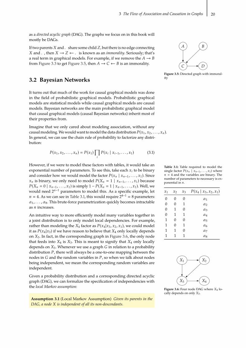
3 The Flow of Association and Causation in Graphs 20
� �
� �
Figure 3.5: Directed graph with immoral-
ity
as a directed acyclic graph (DAG). The graphs we focus on in this book will
mostly be DAGs.
If twoparents- and. share some child/, but there is no edge connecting
- and ., then - → /← . is known as an immorality. Seriously; that’sa real term in graphical models. For example, if we remove the �→ �
from Figure 3.3 to get Figure 3.5, then �→ � ← � is an immorality.
3.2 Bayesian Networks
It turns out that much of the work for causal graphical models was done
in the field of probabilistic graphical models. Probabilistic graphical
models are statistical models while causal graphical models are causal
models. Bayesian networks are the main probabilistic graphical model
that causal graphical models (causal Bayesian networks) inherit most of
their properties from.
Imagine that we only cared about modeling association, without any
causalmodeling.Wewouldwant tomodel thedatadistribution%(G1 , G2 , . . . , G=).In general, we can use the chain rule of probability to factorize any distri-
bution:
%(G1 , G2 , . . . , G=) = %(G1)∏8
%(G8 | G8−1 , . . . , G1) (3.1)
However, if we were to model these factors with tables, it would take an
exponential number of parameters. To see this, take each G8 to be binary
and consider how we would model the factor %(G= | G=−1 , . . . , G1). SinceG= is binary, we only need to model %(-= = 1 | G=−1 , . . . , G1) because%(-= = 0 | G=−1 , . . . , G1) is simply 1− %(-= = 1 | G=−1 , . . . , G1). Well, we
would need 2=−1
parameters to model this. As a specific example, let
= = 4. As we can see in Table 3.1, this would require 24−1 = 8 parameters:
1 , . . . , 8. This brute-force parametrization quickly becomes intractable
as = increases.
Table 3.1: Table required to model the
single factor %(G= | G=−1 , . . . , G1) where
= = 4 and the variables are binary. The
number of parameters to necessary is ex-
ponential in =.
G1 G2 G3 %(G4 | G3 , G2 , G1)0 0 0 1
0 0 1 2
0 1 0 3
0 1 1 4
1 0 0 5
1 0 1 6
1 1 0 7
1 1 1 8
An intuitive way to more efficiently model many variables together in
a joint distribution is to only model local dependencies. For example,
rather than modeling the -4 factor as %(G4 |G3 , G2 , G1), we could model
it as %(G4 |G3) if we have reason to believe that -4 only locally depends
on -3. In fact, in the corresponding graph in Figure 3.6, the only node
that feeds into -4 is -3. This is meant to signify that -4 only locally
depends on -3. Whenever we use a graph � in relation to a probability
distribution %, there will always be a one-to-one mapping between the
nodes in � and the random variables in %, so when we talk about nodes
being independent, we mean the corresponding random variables are
independent.
-1 -2
-3 -4
Figure 3.6: Four node DAG where -4 lo-
cally depends on only -3.
Given a probability distribution and a corresponding directed acyclic
graph (DAG), we can formalize the specification of independencies with
the local Markov assumption:
Assumption 3.1 (Local Markov Assumption) Given its parents in theDAG, a node - is independent of all its non-descendants.

3 The Flow of Association and Causation in Graphs 21
1A probability distribution is said to be
(locally) Markov with respect to a DAG if
they satisfy the local Markov assumption.
[13]: Koller and Friedman (2009), Proba-bilistic Graphical Models: Principles and Tech-niques
This assumption (along with specific DAGs) gives us a lot. We will
demonstrate this in the next few equations. In our four variable example,
the chain rule of probability tells us that we can factorize any % such that
%(G1 , G2 , G3 , G4) = %(G1)%(G2 | G1)%(G3 | G2 , G1)%(G4 | G3 , G2 , G1) .(3.2)
If % is Markov with respect to the graph1in Figure 3.6, then we can
simplify the last factor:
%(G1 , G2 , G3 , G4) = %(G1)%(G2 | G1)%(G3 | G2 , G1)%(G4 | G3) . (3.3)
If we further remove edges, removing -1 → -2 and -2 → -3 as in
Figure 3.7, we can further simplify the factorization of %:
%(G1 , G2 , G3 , G4) = %(G1)%(G2)%(G3 | G1)%(G4 | G3) . (3.4)
-1 -2
-3 -4
Figure 3.7: Four node DAG with even
more independencies.
With the understanding that we have hopefully built up from a few
examples,2
2Active reading exercise:: ensure that you
know how we get from Equation 3.2 to
Equation 3.3 and to Equation 3.4 using the
local Markov assumption.
we will now state one of the main consequences of the local
Markov assumption:
Definition 3.1 (Bayesian Network Factorization) Given a probabilitydistribution % and a DAG �, % factorizes according to � if
%(G1 , . . . , G=) =∏8
%(G8 | pa8)
Hopefully you see the resemblance between the move from Equation 3.2
to Equation 3.3 or the move to Equation 3.4 and the generalization of this
that is presented in Definition 3.1.
The Bayesian network factorization is also known as the chain rule forBayesian networks or Markov compatibility. For example, if % factorizes
according to �, then % and � are Markov compatible.
We have given the intuition of how the local Markov assumption implies
the Bayesian network factorization, and it turns out that the two are
actually equivalent. In other words, we could have started with the
Bayesian network factorization as the main assumption (and labeled it as
an assumption) and shown that it implies the local Markov assumption.
See Koller and Friedman [13, Chapter 3] for these proofs and more
information on this topic.
As important as the local Markov assumption is, it only gives us infor-
mation about the independencies in % that a DAG implies. It does not
even tell us that if - and . are adjacent in the DAG, then - and . are
dependent. And this additional information is very commonly assumed
in causal DAGs. To get this guaranteed dependence between adjacent
nodes, we will generally assume a slightly stronger assumption than the
local Markov assumption: minimality.
Assumption 3.2 (Minimality Assumption) 1. Given its parents inthe DAG, a node - is independent of all its non-descendants (Assump-tion 3.1).
2. Adjacent nodes in the DAG are dependent.3
3This is often equivalently stated in the
following way: if we were to remove any
edges from the DAG, % would not be
Markov with respect to the graph with
the removed edges [see, e.g., 14, Section
6.5.3]
[14]: Peters et al. (2017), Elements of CausalInference: Foundations and Learning Algo-rithms
.

3 The Flow of Association and Causation in Graphs 22
4Active reading exercise: why is removing
edges in a Bayesian network equivalent to
adding independencies?
To see why this assumption is named “minimality” consider, what we
knowwhenwe know that % is Markovwith respect to a DAG�. We know
that % satisfies a set of independencies that are specific to the structure of
�. If % and � also satisfy minimality, then this set of independencies is
minimal in the sense the % does not satisfy any additional independencies.
This is equivalent to saying that adjacent nodes are dependent.
For example, if the DAG were simply two connected nodes - and . as
in Figure 3.8, the local Markov assumption would tell us that we can
factorize %(G, H) as %(G)%(H |G), but it would also allow us to factorize
%(G, H) as %(G)%(H), meaning it allows distributions where - and . are
independent. In contrast, the minimality assumption does not allow this
additional independence. Minimality would tell us to factorize %(G, H)as %(G)%(H |G), and it would tell us that no additional independencies
(- ⊥⊥ .) exist in % that are minimal with respect to Figure 3.8.
- .
Figure 3.8: Two connected nodes
Because removing edges in a Bayesian network is equivalent to adding
independencies,4the minimality assumption is equivalent to saying that
we can’t remove any more edges from the graph. In a sense, every edge is
“active.” More concretely, consider that % and � are Markov compatible
and that �′ is what we get when we remove some edge from �. If % is
also Markov with respect to �′, then % is not minimal with respect to
�.
Armed with the minimality assumption and what it implies about how
distributions factorize when they are Markov with respect to some DAG
(Definition 3.1), we are now ready to discuss the flow of association in
DAGs. However, because everything in this section is purely statistical,
we are not ready to discuss the flow of causation in DAGs. To do that, we
must make causal assumptions. Pedagogically, this will also allow us to
use intuitive causal language when we explain the flow of association.
3.3 Causal Graphs
The previous section was all about statistical models and modeling
association. In this section, we will augment these models with causal
assumptions, turning them into causal models and allowing us to study
causation. In order to introduce causal assumptions, we must first have
an understanding of what it means for - to be a cause of ..
Definition 3.2 (What is a cause?) A variable - is said to be a cause of avariable . if . can change in response to changes in -.5 5
See Section 4.5.1 for a definition using
mathematical notation.
Another phrase commonly used to describe this primitive is that .
“listens” to - . With this, we can now specify the main causal assumption
that we will use throughout this book.
Assumption 3.3 ((Strict) Causal Edges Assumption) In a directed graph,every parent is a direct cause of all its children.
Here, the set of direct causes of . is everything that . directly responds
to; if we fix all of the direct causes of ., then changing any other cause of
. won’t induce any changes in .. This assumption is “strict” in the sense

3 The Flow of Association and Causation in Graphs 23
that every edge is “active,” just like in DAGs that satisfy minimality. In
other words, because the definition of a cause (Definition 3.2) implies
that a cause and its effect are dependent and because we are assuming
all parents are causes of their children, we are assuming that parents
and their children are dependent. So the second part of minimality
(Assumption 3.2) is baked into the strict causal edges assumption.
In contrast, the non-strict causal edges assumption would allow for
some parents to not be causes of their children. It would just assume
that children are not causes of their parents. This allows us to draw
graphs with extra edges to make fewer assumptions, just like we would
in Bayesian networks, where more edges means fewer independence
assumptions. Causal graphs are sometimes drawn with this kind of
non-minimal meaning, but the vast majority of the time, when someone
draws a causal graph, they mean that parents are causes of their children.
Therefore, unless we specify otherwise, throughout this book, we will
use “causal graph” to refer to a DAG that satisfies the strict causal edges
assumption. And we will often omit the word “strict” when we refer to
this assumption.
When we add the causal edges assumption, directed paths in the DAG
take on a very special meaning; they correspond to causation. This is in
contrast to other paths in the graph, which association may flow along,
but causation certainly may not. This will become more clear when we
go into detail on these other kinds of paths in Sections 3.5 and 3.6.
Moving forward, we will now think of the edges of graphs as causal, in
order to describe concepts intuitively with causal language. However,
all of the associational claims about statistical independence will still
hold, even when the edges do not have causal meaning like in the vanilla
Bayesian networks of Section 3.2.
As we will see in the next few sections, the main assumptions that we
need for our causal graphical models to tell us how association and
causation flow between variables are the following two:
1. Local Markov Assumption (Assumption 3.1)
2. Causal Edges Assumption (Assumption 3.3)
We will discuss these assumptions throughout the next few sections and
come back to discuss them more fully again in Section 3.8 after we’ve
established the necessary preliminaries.
3.4 Two-Node Graphs and Graphical BuildingBlocks
Now that we’ve gotten the basic assumptions and definitions out of the
way, we can get to the core of this chapter: the flow of association and
causation in DAGs. We can understand this flow in general DAGs by
understanding the flow in the minimal building blocks of graphs. These
minimal building blocks consist of chains (Figure 3.9a), forks (Figure 3.9b),
immoralities (Figure 3.9c), two unconnected nodes (Figure 3.10), and two
connected nodes (Figure 3.11).

3 The Flow of Association and Causation in Graphs 24
-1 -2 -3
(a) Chain
-2
-1 -3
(b) Fork
-1
-2
-3
(c) Immorality
Figure 3.9: Basic graph building blocks
-1 -2
Figure 3.11: Two connected nodes
6Two adjacent nodes in a non-strict causal
graph can be unassociated.
-1 -2 -3
Figure 3.12:Chainwithflowof association
drawn as a dashed red arc.
By “flow of association,” we mean whether any two nodes in a graph are
associated or not associated. Another way of saying this is whether two
nodes are (statistically) dependent or (statistically) independent. Addi-
tionally, we will study whether two nodes are conditionally independent
or not.
For each building block, we will give the intuition for why two nodes
are (conditionally) independent or not, and we will give a proof as well.
We can prove that two nodes � and � are conditionally independent
given some set of nodes � by simply showing that %(0, 1 |2) factorizesas %(0 |2)%(1 |2). We will now do this in the case of the simplest basic
building block: two unconnected nodes.
Given a graph that is just two unconnected nodes, as depicted in Fig-
ure 3.10, these nodes are not associated simply because there is no edge
between them. To show this, consider the factorization of %(G1 , G2) thatthe Bayesian network factorization (Definition 3.1) gives us:
%(G1 , G2) = %(G1)%(G2) (3.5)
That’s it; applying the Bayesian network factorization immediately gives
us a proof that the two nodes -1 and -2 are unassociated (independent)
in this building block. And what is the assumption that allows us to
prove this? That % is Markov with respect to the graph in Figure 3.10.
-1 -2
Figure 3.10: Two unconnected nodes
In contrast, if there is an edge between the two nodes (as in Figure 3.11),
then the two nodes are associated. The assumption we leverage here is
the causal edges assumption (Assumption 3.3), which means that -1
is a cause of -2. Since -1 is a cause of -2, -2 must be able to change
in response to changes in -1, so -2 and -1 are associated. In general,
any time two nodes are adjacent in a causal graph, they are associated.6
We will see this same concept several more times in Section 3.5 and
Section 3.6.
Now that we’ve covered the relevant two-node graphs, we’ll cover the
flowof association in the remaining graphical building blocks (three-node
graphs in Figure 3.9), starting with chain graphs.
3.5 Chains and Forks
Chains (Figure 3.12) and forks (Figure 3.13) share the same set of depen-
dencies. In both structures, -1 and -2 are dependent, and -2 and -3
are dependent for the same reason that we discussed toward the end
of Section 3.4. Adjacent nodes are always dependent when we make
the causal edges assumption (Assumption 3.3). What about -1 and -3,
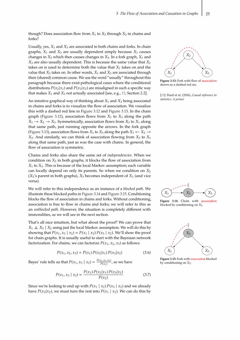
3 The Flow of Association and Causation in Graphs 25
-2
-1 -3
Figure 3.13: Fork with flow of association
drawn as a dashed red arc.
[15]: Pearl et al. (2016), Causal inference instatistics: A primer
-2-1 -3
Figure 3.14: Chain with association
blocked by conditioning on -2.
-2
-1 -3
Figure 3.15: Fork with association blocked
by conditioning on -2.
though? Does association flow from -1 to -3 through -2 in chains and
forks?
Usually, yes, -1 and -3 are associated in both chains and forks. In chain
graphs, -1 and -3 are usually dependent simply because -1 causes
changes in -2 which then causes changes in -3. In a fork graph, -1 and
-3 are also usually dependent. This is because the same value that -2
takes on is used to determine both the value that -1 takes on and the
value that -3 takes on. In other words, -1 and -3 are associated through
their (shared) common cause. We use the word “usually” throughout this
paragraph because there exist pathological cases where the conditional
distributions %(G2 |G1) and %(G3 |G2) are misaligned in such a specific way
that makes -1 and -3 not actually associated [see, e.g., 15, Section 2.2].
An intuitive graphical way of thinking about -1 and -3 being associated
in chains and forks is to visualize the flow of association. We visualize
this with a dashed red line in Figure 3.12 and Figure 3.13. In the chain
graph (Figure 3.12), association flows from -1 to -3 along the path
-1 → -2 → -3. Symmetrically, association flows from -3 to -1 along
that same path, just running opposite the arrows. In the fork graph
(Figure 3.13), association flows from -1 to -3 along the path -1 ← -2 →-3. And similarly, we can think of association flowing from -3 to -1
along that same path, just as was the case with chains. In general, the
flow of association is symmetric.
Chains and forks also share the same set of independencies. When we
condition on -2 in both graphs, it blocks the flow of association from
-1 to -3. This is because of the local Markov assumption; each variable
can locally depend on only its parents. So when we condition on -2
(-3’s parent in both graphs), -3 becomes independent of -1 (and vice
versa).
We will refer to this independence as an instance of a blocked path. We
illustrate these blocked paths in Figure 3.14 and Figure 3.15. Conditioning
blocks the flow of association in chains and forks. Without conditioning,
association is free to flow in chains and forks; we will refer to this as
an unblocked path. However, the situation is completely different with
immoralities, as we will see in the next section.
That’s all nice intuition, but what about the proof? We can prove that
-1 ⊥⊥ -3 | -2 using just the local Markov assumption. We will do this by
showing that %(G1 , G3 | G2) = %(G1 | G2)%(G3 | G2). We’ll show the proof
for chain graphs. It is usually useful to start with the Bayesian network
factorization. For chains, we can factorize %(G1 , G2 , G3) as follows:
%(G1 , G2 , G3) = %(G1)%(G2 |G1)%(G3 |G2) (3.6)
Bayes’ rule tells us that %(G1 , G3 | G2) = %(G1 ,G2 ,G3)%(G2) , so we have
%(G1 , G3 | G2) =%(G1)%(G2 |G1)%(G3 |G2)
%(G2)(3.7)
Since we’re looking to end up with %(G1 | G2)%(G3 | G2) and we already
have %(G3 |G2), we must turn the rest into %(G1 | G2). We can do this by

3 The Flow of Association and Causation in Graphs 26
7Active reading exercise: prove that
-1 ⊥⊥ -3 | -2 for forks (Figure 3.15).
-2
-1-3
Figure 3.16: Immorality with association
blocked by a collider.
-2
-1-3
Figure 3.17: Immorality with association
unblocked by conditioning on the collider.
another application of Bayes rule:
%(G1 , G3 | G2) =%(G1 , G2)%(G2)
%(G3 |G2) (3.8)
= %(G1 |G2)%(G3 |G2) (3.9)
With that, we’ve shown that -1 ⊥⊥ -3 | -2. Try it yourself; prove the
analog in forks.7
Flow of Causation The flow of association is symmetric, whereas the
flow of causation is not. Under the causal edges assumption (Assump-
tion 3.3), causation only flows in a single direction. Causation only flows
along directed paths. Association flows along any path that does not
contain an immorality.
3.6 Colliders and their Descendants
Recall from Section 3.1 that we have an immorality when we have a child
whose two parents do not have an edge connecting them (Figure 3.16).
And in this graph structure, the child is known as a bastard. No, just
kidding; it’s called a collider.
In contrast to chains and forks, in an immorality, -1 ⊥⊥ -3. Look at
the graph structure and think about it a bit. Why would -1 and -3 be
associated? One isn’t the descendant of the other like in chains, and
they don’t share a common cause like in forks. Rather, we can think of
-1 and -3 simply as unrelated events that happen, which happen to
both contribute to some common effect (-2). To show this, we apply the
Bayesian network factorization and marginalize out G2:
%(G1 , G3) =∑G2
%(G1 , G2 , G3) (3.10)
=∑G2
%(G1)%(G3)%(G2 | G1 , G3) (3.11)
= %(G1)%(G3)∑G2
%(G2 | G1 , G3) (3.12)
= %(G1)%(G3) (3.13)
We illustrate the independence of -1 and -3 in Figure 3.16 by showing
that the association that we could have imagined as flowing along the
path -1 → -2 ← -3 is actually blocked at -2. Because we have a collider
on the path connecting -1 and -3, association does not flow through
that path. This is another example of a blocked path, but this time the path
is not blocked by conditioning; the path is blocked by a collider.
Good-Looking Men are Jerks Oddly enough, when we condition on
the collider -2, its parents -1 and -3 become dependent (depicted
in Figure 3.17). An example is the easiest way to see why this is the
case. Imagine that you’re out dating men, and you notice that most
of the nice men you meet are not very good-looking, and most of the
good-looking men you meet are jerks. It seems that you have to choose
between looks and kindness. In other words, it seems like kindness and
looks are negatively associated. However, what if I also told you that
there is an important third variable here: availability (whether men are
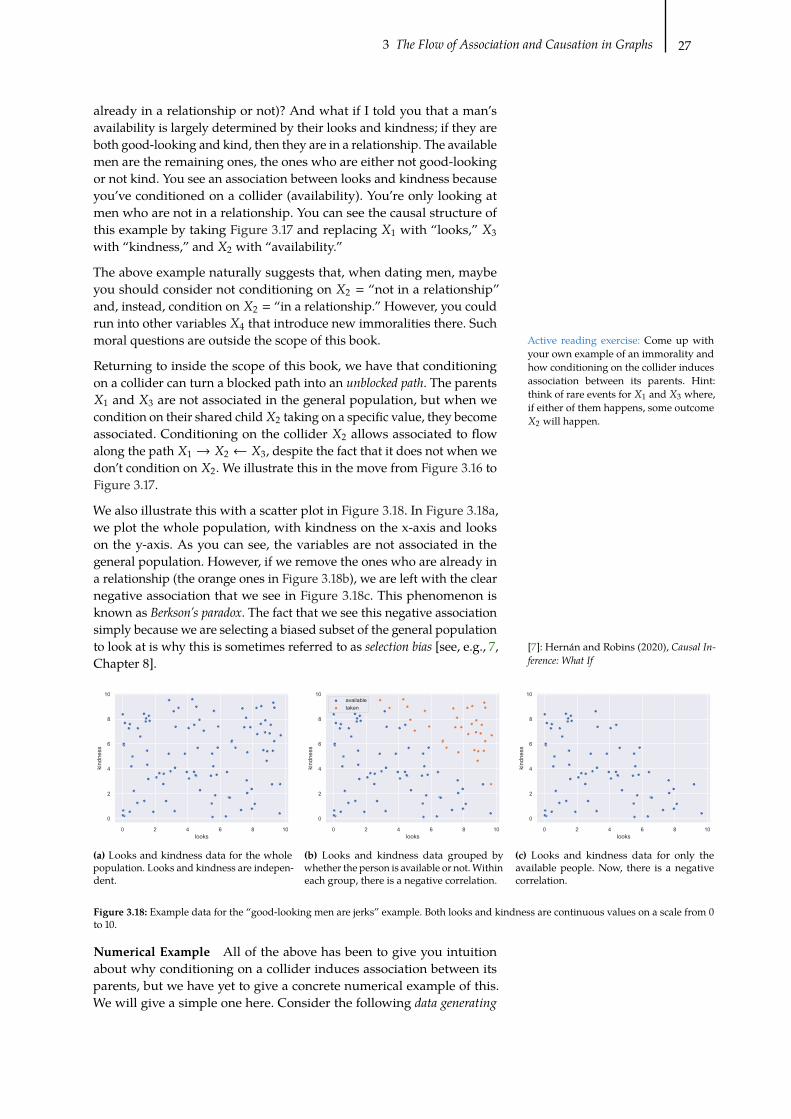
3 The Flow of Association and Causation in Graphs 27
Active reading exercise: Come up with
your own example of an immorality and
how conditioning on the collider induces
association between its parents. Hint:
think of rare events for -1 and -3 where,
if either of them happens, some outcome
-2 will happen.
already in a relationship or not)? And what if I told you that a man’s
availability is largely determined by their looks and kindness; if they are
both good-looking and kind, then they are in a relationship. The available
men are the remaining ones, the ones who are either not good-looking
or not kind. You see an association between looks and kindness because
you’ve conditioned on a collider (availability). You’re only looking at
men who are not in a relationship. You can see the causal structure of
this example by taking Figure 3.17 and replacing -1 with “looks,” -3
with “kindness,” and -2 with “availability.”
The above example naturally suggests that, when dating men, maybe
you should consider not conditioning on -2 = “not in a relationship”
and, instead, condition on -2 = “in a relationship.” However, you could
run into other variables -4 that introduce new immoralities there. Such
moral questions are outside the scope of this book.
Returning to inside the scope of this book, we have that conditioning
on a collider can turn a blocked path into an unblocked path. The parents-1 and -3 are not associated in the general population, but when we
condition on their shared child-2 taking on a specific value, they become
associated. Conditioning on the collider -2 allows associated to flow
along the path -1 → -2 ← -3, despite the fact that it does not when we
don’t condition on -2. We illustrate this in the move from Figure 3.16 to
Figure 3.17.
We also illustrate this with a scatter plot in Figure 3.18. In Figure 3.18a,
we plot the whole population, with kindness on the x-axis and looks
on the y-axis. As you can see, the variables are not associated in the
general population. However, if we remove the ones who are already in
a relationship (the orange ones in Figure 3.18b), we are left with the clear
negative association that we see in Figure 3.18c. This phenomenon is
known as Berkson’s paradox. The fact that we see this negative association
simply because we are selecting a biased subset of the general population
to look at is why this is sometimes referred to as selection bias [see, e.g., 7,Chapter 8]
[7]: Hernán and Robins (2020), Causal In-ference: What If
.
0 2 4 6 8 10looks
0
2
4
6
8
10
kind
ness
(a) Looks and kindness data for the whole
population. Looks and kindness are indepen-
dent.
0 2 4 6 8 10looks
0
2
4
6
8
10
kind
ness
availabletaken
(b) Looks and kindness data grouped by
whether the person is available or not.Within
each group, there is a negative correlation.
0 2 4 6 8 10looks
0
2
4
6
8
10
kind
ness
(c) Looks and kindness data for only the
available people. Now, there is a negative
correlation.
Figure 3.18: Example data for the “good-looking men are jerks” example. Both looks and kindness are continuous values on a scale from 0
to 10.
Numerical Example All of the above has been to give you intuition
about why conditioning on a collider induces association between its
parents, but we have yet to give a concrete numerical example of this.
We will give a simple one here. Consider the following data generating

3 The Flow of Association and Causation in Graphs 28
process (DGP), where -1 and -3 are drawn independently from standard
normal distributions and then used to compute -2:
-1 ∼ #(0, 1) , -3 ∼ #(0, 1) (3.14)
-2 = -1 + -3 (3.15)
We’ve already stated that -1 and -3 are independent, but to juxtapose
the two calculations, let’s compute their covariance:
Cov(-1 , -3) = E[(-1 − E[-1])(-3 − E[-3])]= E[-1-3] (zero mean)
= E[-1]E[-3] (independent)
= 0
Now, let’s compute their covariance, conditional on -2:
Cov(-1 , -3 | -2 = G) = E[-1-3 | -2 = G] (3.16)
= E[-1(G − -1)] (3.17)
= GE[-1] − E[-2
1] (3.18)
= −1 (3.19)
Crucially, in Equation 3.17, we used Equation 3.15 to plug in for -3 in
terms of -1 and -2 (conditioned to G). This led to a second-order term,
which led to the calculation giving a nonzero number, which means -1
and -3 are associated, conditional on -2.
Descendants of Colliders Conditioning on descendants of a collider
also induces association in between the parents of the collider. The
intuition is that if we learn something about a collider’s descendant, we
usually also learn something about the collider itself because there is
a direct causal path from the collider to its descendants, and we know
that nodes in a chain are usually associated (see Section 3.5), assuming
minimality (Assumption 3.2). In other words, a descendant of a collider
can be thought of as a proxy for that collider, so conditioning on the
descendant is similar to conditioning on the collider itself.
Active reading exercise:We have provided
several techniques for how to think about
colliders: high-level examples, numerical
examples, and abstract reasoning. Use at
least one of them to convince yourself
that conditioning on a descendant of a
collider can induce association between
the collider’s parents.3.7 d-separation
Before we define d-separation, we’ll codify what we mean by the con-
cept of a “blocked path,” which we’ve been discussing in the previous
sections:
Definition 3.3 (blocked path) A path between nodes - and . is blockedby a (potentially empty) conditioning set / if either of the following is true:
1. Along the path, there is a chain · · · →, → · · · or a fork· · · ←, → · · ·, where, is conditioned on (, ∈ /).
2. There is a collider, on the path that is not conditioned on (, ∉ /)and none of its descendants are conditioned on (de(,) * /).
Then, an unblocked path is simply the complement; an unblocked path is a

3 The Flow of Association and Causation in Graphs 29
[13]: Koller and Friedman (2009), Proba-bilistic Graphical Models: Principles and Tech-niques
path that is not blocked. The graphical intuition to have in mind is that
association flows along unblocked paths, and association does not flow
along blocked paths. If you don’t have this intuition in mind, then it is
probably worth it to reread the previous two sections, with the goal of
gaining this intuition. Now, we are ready to introduce a very important
concept: d-separation.
Definition 3.4 (d-separation) Two (sets of) nodes - and . are d-separatedby a set of nodes / if all of the paths between (any node in) - and (any nodein) . are blocked by / [16] [16]: Pearl (1988), Probabilistic Reasoning
in Intelligent Systems: Networks of PlausibleInference
.
If all the paths between two nodes - and . are blocked, then we say that
- and. are d-separated. Similarly, if there exists at least one path between
- and . that is unblocked, then we say that - and . are d-connected.
As we will see in Theorem 3.1, d-separation is such an important concept
because it implies conditional independence. We will use the notation
- ⊥⊥� . | / to denote that - and . are d-separated in the graph �
when conditioning on /. Similarly, we will use the notation - ⊥⊥% . | /to denote that - and . are independent in the distribution % when
conditioning on /.
Theorem 3.1 Given that % is Markov with respect to � (satisfies the localMarkov assumption, Assumption 3.1), if - and . are d-separated in �conditioned on /, then - and . are independent in % conditioned on /. Wecan write this succinctly as follows:
- ⊥⊥� . | / =⇒ - ⊥⊥% . | / (3.20)
Because this is so important, we will give Equation 3.20 a name: the globalMarkov assumption. Theorem 3.1 tells us that the local Markov assumption
implies the global Markov assumption.
Just as we built up the intuition that suggested that the local Markov
assumption (Assumption 3.1) implies the Bayesian network factorization
(Definition 3.1) and alerted you to the fact that the Bayesian network
factorization also implies the local Markov assumption (the two are equiv-
alent), it turns out that the global Markov assumption also implies the
local Markov assumption. In other words, the local Markov assumption,
global Markov assumption, and the Bayesian network factorization are
all equivalent [see, e.g., 13, Chapter 3]. Therefore, we will use the slightly
shortened phrase Markov assumption to refer to these concepts as a
group, or we will simply write “% is Markov with respect to �” to convey
the same meaning.
Active reading exercise: To get some practice with d-separation, here are
some questions about d-separation in Figure 3.19.
Questions about Figure 3.19a:
1. Are ) and . d-separated by the empty set?
2. Are ) and . d-separated by,2?
3. Are ) and . d-separated by {,2 , "1}?4. Are ) and . d-separated by {,1 , "2}?5. Are ) and . d-separated by {,1 , "2 , -2}?

3 The Flow of Association and Causation in Graphs 30
6. Are ) and . d-separated by {,1 , "2 , -2 , -3}?
Questions about Figure 3.19b:
1. Are ) and . d-separated by the empty set?
2. Are ) and . d-separated by,?
3. Are ) and . d-separated by {,, -2}?
) "1 "2 .
,1
,2
,3
-3
-2
-1
(a)
)
-1
.
,
-2
(b)
Figure 3.19: Graphs for d-separation exercise
3.8 Flow of Association and Causation
Now that we have covered the necessary preliminaries (chains, forks,
colliders, and d-separation), it is worth emphasizing how association and
causation flow in directed graphs. Association flows along all unblocked
paths. In causal graphs, causation flows along directed paths. Recall from
Section 1.3.2 that not only is association not causation, but causation is a
sub-category of association. That’s why association and causation both
flow along directed paths.
We refer to the flowof association along directed paths as causal association.A common type of non-causal association that makes total association
not causation is confounding association. In the graph in Figure 3.20, we
depict the confounding association in red and the causal association in
blue.
-
) .
confounding association
causal association
Figure 3.20: Causal graph depicting an
example of how confounding association
and causal association flow.
Regular Bayesian networks are purely statistical models, so we can only
talk about the flow of association in Bayesian networks. Association still
flows in exactly the same way in Bayesian networks as it does in causal
graphs, though. In both, association flows along chains and forks, unless
a node is conditioned on. And in both, a collider blocks the flow of
association, unless it is conditioned on. Combining these building blocks,
we get how association flows in general DAGs. We can tell if two nodes
are not associated (no association flows between them) by whether or
not they are d-separated.
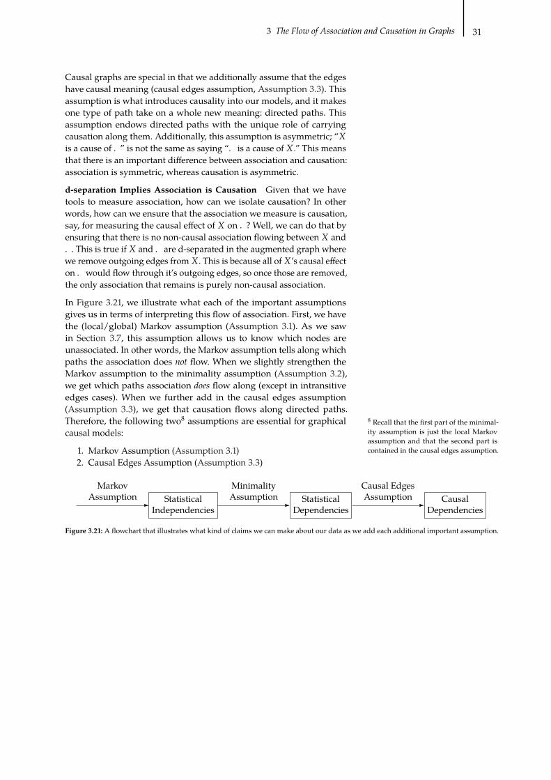
3 The Flow of Association and Causation in Graphs 31
8Recall that the first part of the minimal-
ity assumption is just the local Markov
assumption and that the second part is
contained in the causal edges assumption.
Causal graphs are special in that we additionally assume that the edges
have causal meaning (causal edges assumption, Assumption 3.3). This
assumption is what introduces causality into our models, and it makes
one type of path take on a whole new meaning: directed paths. This
assumption endows directed paths with the unique role of carrying
causation along them. Additionally, this assumption is asymmetric; “-
is a cause of .” is not the same as saying “. is a cause of - .” This means
that there is an important difference between association and causation:
association is symmetric, whereas causation is asymmetric.
d-separation Implies Association is Causation Given that we have
tools to measure association, how can we isolate causation? In other
words, how can we ensure that the association we measure is causation,
say, for measuring the causal effect of - on .? Well, we can do that by
ensuring that there is no non-causal association flowing between - and
.. This is true if - and . are d-separated in the augmented graph where
we remove outgoing edges from - . This is because all of -’s causal effect
on . would flow through it’s outgoing edges, so once those are removed,
the only association that remains is purely non-causal association.
In Figure 3.21, we illustrate what each of the important assumptions
gives us in terms of interpreting this flow of association. First, we have
the (local/global) Markov assumption (Assumption 3.1). As we saw
in Section 3.7, this assumption allows us to know which nodes are
unassociated. In other words, the Markov assumption tells along which
paths the association does not flow. When we slightly strengthen the
Markov assumption to the minimality assumption (Assumption 3.2),
we get which paths association does flow along (except in intransitive
edges cases). When we further add in the causal edges assumption
(Assumption 3.3), we get that causation flows along directed paths.
Therefore, the following two8assumptions are essential for graphical
causal models:
1. Markov Assumption (Assumption 3.1)
2. Causal Edges Assumption (Assumption 3.3)
Statistical
Independencies
Statistical
Dependencies
Causal
Dependencies
Markov
Assumption
Minimality
Assumption
Causal Edges
Assumption
Figure 3.21: A flowchart that illustrates what kind of claims we can make about our data as we add each additional important assumption.

Causal Models 44.1 The do-operator and Inter-
ventional Distributions . . 324.2 TheMainAssumption:Mod-
ularity . . . . . . . . . . . . . 344.3 Truncated Factorization . . 35
ExampleApplication andRe-visiting “Association is NotCausation” . . . . . . . . . . 36
4.4 The Backdoor Adjustment 37Relation to Potential Out-comes . . . . . . . . . . . . . 39
4.5 Structural Causal Models(SCMs) . . . . . . . . . . . . 40
Structural Equations . . . . 40Interventions . . . . . . . . . 42ColliderBias andWhy toNotCondition on Descendantsof Treatment . . . . . . . . . 43
4.6 Example Applications of theBackdoor Adjustment . . . 44
Association vs. Causation ina Toy Example . . . . . . . . 44
A Complete Example withEstimation . . . . . . . . . . 45
4.7 Assumptions Revisited . . . 47
Causal models are essential for identification of causal quantities. When
we presented the Identification-Estimation Flowchart (Figure 2.5) back
in Section 2.4, we described identification as the process of moving
from a causal estimand to a statistical estimand. However, to do that,
we must have a causal model. We depict this more full version of the
Identification-Estimation Flowchart in Figure 4.1.
Causal Estimand Causal Model
Statistical Estimand Data
Estimate
Figure 4.1: The Identification-Estimation Flowchart – a flowchart that illustrates the process
of moving from a target causal estimand to a corresponding estimate, through identification
and estimation. In contrast to Figure 2.5, this version is augmented with a causal model
and data.
The previous chapter gives graphical intuition for causal models, but it
doesn’t explain how to identify causal quantities and formalize causal
models. We will do that in this chapter.
4.1 The do-operator and InterventionalDistributions
The first thing that we will introduce is a mathematical operator for
intervention. In the regular notation for probability, we have conditioning,
but that isn’t the same as intervening. Conditioning on ) = C just means
that we are restricting our focus to the subset of the population to those
who received treatment C. In contrast, an intervention would be to take
the whole population and give everyone treatment C. We illustrate this in
Figure 4.2. We will denote intervention with the do-operator: do() = C).This is the notation commonly used in graphical causal models, and it has
equivalents in potential outcomes notation. For example, we can write
the distribution of the potential outcome .(C) that we saw in Chapter 2
as follows:
%(.(C) = H) , %(. = H | do() = C)) , %(H | do(C)) (4.1)
Note that we shorten do() = C) to just do(C) in the last option in Equation
4.1. We will use this shorthand throughout the book. We can similarly
write the ATE (average treatment effect) when the treatment is binary as
follows:
E[. | do() = 1)] − E[. | do() = 0)] (4.2)

4 Causal Models 33
Population Conditioning InterveningSubpopulations
oror
) = 1) = 1) = 0
) = 0
do() = 1)
do() = 0)
Figure 4.2: Illustration of the difference between conditioning and intervening
We will often work with full distributions like %(. | do(C)), rather thantheir means, as this is more general; if we characterize %(. | do(C)), thenwe’ve characterized E[. | do(C)]. We will commonly refer to %(. | do() =
C)) and other expressions with the do-operator in them as interventionaldistributions.
Interventional distributions such as %(. | do() = C)) are conceptually
quite different from the observational distribution %(.). Observational
distributions such as %(.) or %(., ), -) do not have the do-operator inthem. Because they don’t have the do-operator, we can observe data from
them without needing to carry out any experiment. This is why we call
data from %(., ), -) observational data. If we can reduce an expression
& with do in it (an interventional expression) to one without do in it (an
observational expression), then & is said to be identifiable. An expression
with a do in it is fundamentally different from an expression without a
do in it, despite the fact that in do-notation, do appears after a regular
conditioning bar. As we discussed in Section 2.4, we will refer to an
estimand as a causal estimand when it contains a do-operator, and we
refer to an estimand as a statistical estimand when it doesn’t contain a
do-operator.
Whenever, do(C) appears after the conditioning bar, it means that ev-
erything in that expression is in the post-intervention world where the
intervention do(C) occurs. For example, E[. | do(C), / = I] refers to the
expected outcome in the subpopulation where / = I after the whole
subpopulation has taken treatment C. In contrast, E[. | / = I] simply
refers to the expected value in the (pre-intervention) population where
individuals take whatever treatment they would normally take ()). This
distinction will become important when we get to counterfactuals in
Chapter 14.
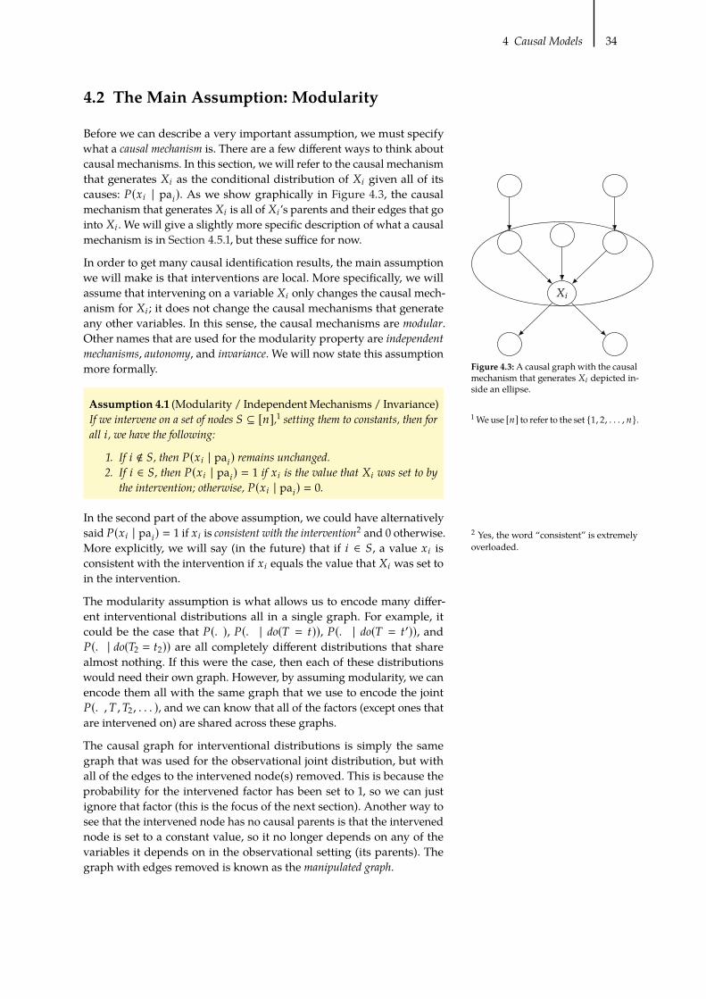
4 Causal Models 34
2Yes, the word “consistent” is extremely
overloaded.
4.2 The Main Assumption: Modularity
Before we can describe a very important assumption, we must specify
what a causal mechanism is. There are a few different ways to think about
causal mechanisms. In this section, we will refer to the causal mechanism
that generates -8 as the conditional distribution of -8 given all of its
causes: %(G8 | pa8). As we show graphically in Figure 4.3, the causal
mechanism that generates -8 is all of -8 ’s parents and their edges that go
into -8 . We will give a slightly more specific description of what a causal
mechanism is in Section 4.5.1, but these suffice for now.
-8
Figure 4.3:A causal graph with the causal
mechanism that generates -8 depicted in-
side an ellipse.
In order to get many causal identification results, the main assumption
we will make is that interventions are local. More specifically, we will
assume that intervening on a variable -8 only changes the causal mech-
anism for -8 ; it does not change the causal mechanisms that generate
any other variables. In this sense, the causal mechanisms are modular.Other names that are used for the modularity property are independentmechanisms, autonomy, and invariance. We will now state this assumption
more formally.
Assumption 4.1 (Modularity / IndependentMechanisms / Invariance)
If we intervene on a set of nodes ( ⊆ [=],1 1Weuse [=] to refer to the set {1, 2, . . . , =}.setting them to constants, then for
all 8, we have the following:
1. If 8 ∉ (, then %(G8 | pa8) remains unchanged.2. If 8 ∈ (, then %(G8 | pa8) = 1 if G8 is the value that -8 was set to by
the intervention; otherwise, %(G8 | pa8) = 0.
In the second part of the above assumption, we could have alternatively
said %(G8 | pa8) = 1 if G8 is consistent with the intervention2 and 0 otherwise.
More explicitly, we will say (in the future) that if 8 ∈ (, a value G8 is
consistent with the intervention if G8 equals the value that -8 was set to
in the intervention.
The modularity assumption is what allows us to encode many differ-
ent interventional distributions all in a single graph. For example, it
could be the case that %(.), %(. | do() = C)), %(. | do() = C′)), and%(. | do()2 = C2)) are all completely different distributions that share
almost nothing. If this were the case, then each of these distributions
would need their own graph. However, by assuming modularity, we can
encode them all with the same graph that we use to encode the joint
%(., ), )2 , . . . ), and we can know that all of the factors (except ones that
are intervened on) are shared across these graphs.
The causal graph for interventional distributions is simply the same
graph that was used for the observational joint distribution, but with
all of the edges to the intervened node(s) removed. This is because the
probability for the intervened factor has been set to 1, so we can just
ignore that factor (this is the focus of the next section). Another way to
see that the intervened node has no causal parents is that the intervened
node is set to a constant value, so it no longer depends on any of the
variables it depends on in the observational setting (its parents). The
graph with edges removed is known as the manipulated graph.

4 Causal Models 35
3The other key principle is the global
Markov assumption (Theorem 3.1), which
is the assumption that d-separation im-
plies conditional independence.
For example, consider the causal graph for an observational distribution
in Figure 4.4a. Both %(. | do() = C)) and %(. | do() = C′)) correspondto the causal graph in Figure 4.4b, where the incoming edge to ) has
been removed. Similarly, %(. | do()2 = C2)) corresponds to the graph
in Figure 4.4c, where the incoming edges to )2 have been removed.
Although it is not expressed in the graphs (which only express conditional
independencies and causal relations), under the modularity assumption,
%(.), %(. | ) = C′), and %(. | do()2 = C2)) all shared the exact same
factors (that are not intervened on).
.
))2
)3
(a) Causal graph for observational distri-
bution
.
))2
)3
(b) Causal graph after intervention on )(interventional distribution)
.
))2
)3
(c) Causal graph after intervention on )2
(interventional distribution)
Figure 4.4: Intervention as edge deletion in causal graphs
What would it mean for the modularity assumption to be violated?
Imagine that you intervene on -8 , and this causes the mechanism that
generates a different node -9 to change; an intervention on -8 changes
%(G 9 | pa9), where 9 ≠ 8. In other words, the intervention is not local to
the node you intervene on; causal mechanisms are not invariant to when
you change other causal mechanisms; the causal mechanisms are not
modular.
This assumption is so important that Judea Pearl refers to a closely
related version (which we will see in Section 4.5.2) as The Law ofCounterfactuals (and Interventions), one of two key principles from
which all other causal results follow.3Incidentally, taking the modularity
assumption (Assumption 4.1) and the Markov assumption (the other key
principle) together gives us causal Bayesian networks. We’ll now move to
one of the important results that follow from these assumptions.
4.3 Truncated Factorization
Recall the Bayesian network factorization (Definition 3.1), which tells us
that if % is Markov with respect to a graph �, then % factorizes as follows:
%(G1 , . . . , G=) =∏8
%(G8 | pa8) (4.3)
where pa8 denotes the parents of -8 in �. Now, if we intervene on some
set of nodes ( and assume modularity (Assumption 4.1), then all of the
factors should remain the same except the factors for-8 ∈ (; those factors
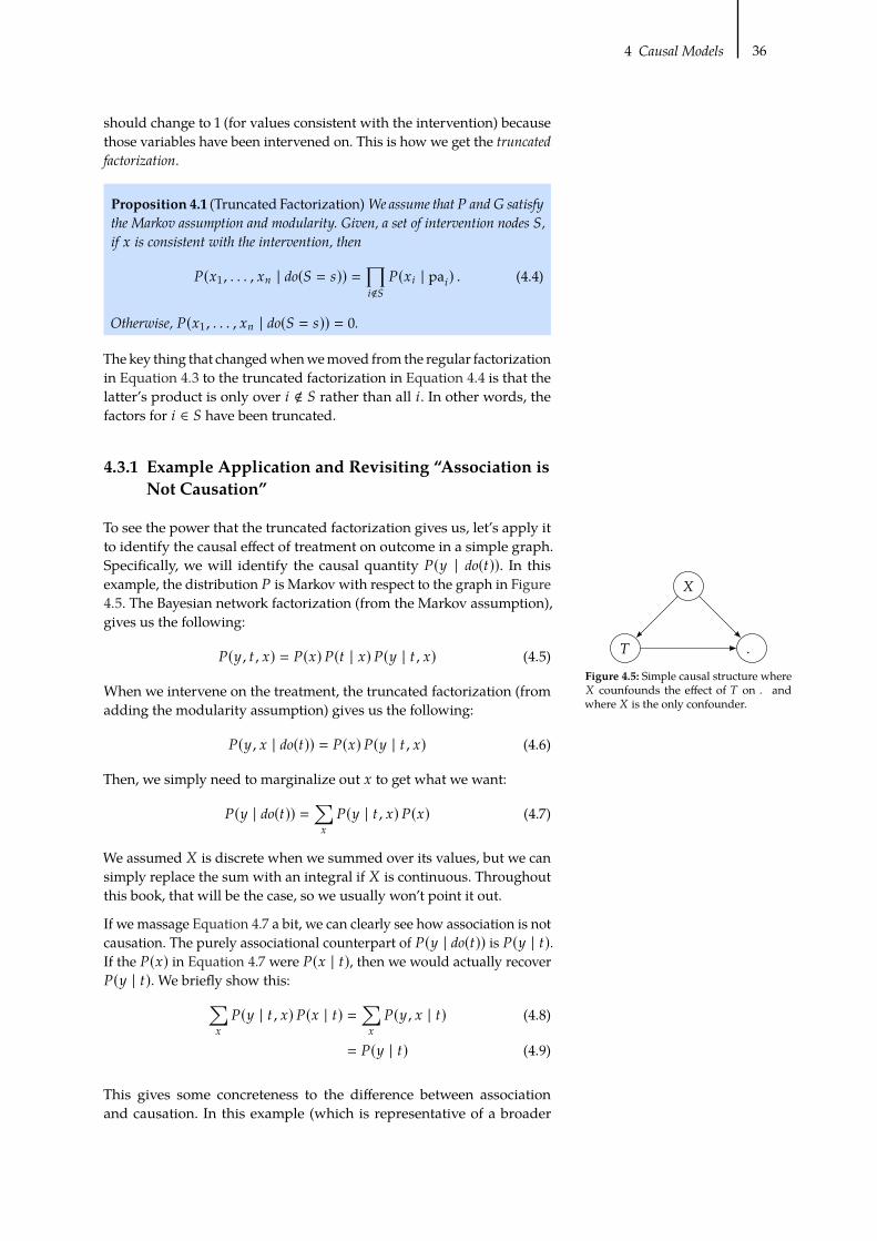
4 Causal Models 36
should change to 1 (for values consistent with the intervention) because
those variables have been intervened on. This is how we get the truncatedfactorization.
Proposition 4.1 (Truncated Factorization) We assume that % and� satisfythe Markov assumption and modularity. Given, a set of intervention nodes (,if G is consistent with the intervention, then
%(G1 , . . . , G= | do(( = B)) =∏8∉(
%(G8 | pa8) . (4.4)
Otherwise, %(G1 , . . . , G= | do(( = B)) = 0.
The key thing that changedwhenwemoved from the regular factorization
in Equation 4.3 to the truncated factorization in Equation 4.4 is that the
latter’s product is only over 8 ∉ ( rather than all 8. In other words, the
factors for 8 ∈ ( have been truncated.
4.3.1 Example Application and Revisiting “Association isNot Causation”
To see the power that the truncated factorization gives us, let’s apply it
to identify the causal effect of treatment on outcome in a simple graph.
Specifically, we will identify the causal quantity %(H | do(C)). In this
example, the distribution % is Markov with respect to the graph in Figure
4.5. The Bayesian network factorization (from the Markov assumption),
gives us the following:
%(H, C, G) = %(G)%(C | G)%(H | C , G) (4.5)
-
) .
Figure 4.5: Simple causal structure where
- counfounds the effect of ) on . and
where - is the only confounder.
When we intervene on the treatment, the truncated factorization (from
adding the modularity assumption) gives us the following:
%(H, G | do(C)) = %(G)%(H | C , G) (4.6)
Then, we simply need to marginalize out G to get what we want:
%(H | do(C)) =∑G
%(H | C , G)%(G) (4.7)
We assumed - is discrete when we summed over its values, but we can
simply replace the sum with an integral if - is continuous. Throughout
this book, that will be the case, so we usually won’t point it out.
If we massage Equation 4.7 a bit, we can clearly see how association is not
causation. The purely associational counterpart of %(H | do(C)) is %(H | C).If the %(G) in Equation 4.7 were %(G | C), then we would actually recover
%(H | C). We briefly show this:∑G
%(H | C , G)%(G | C) =∑G
%(H, G | C) (4.8)
= %(H | C) (4.9)
This gives some concreteness to the difference between association
and causation. In this example (which is representative of a broader

4 Causal Models 37
4Aswementioned in Section 3.8, blocking
all backdoor paths is equivalent to having
d-separation in the graph where edges
going out of) are removed. This is because
these are the only edges that causation
flows along, so once they are removed, all
that remains is non-causation association.
5Active reading exercise: In a generalDAG,
which set of nodes related to) will always
be a sufficient adjustment set? Which set
of nodes related to . will always be a
sufficient adjustment set?
phenomenon), the difference between %(H | do(C)) and %(H | C) is thedifference between %(G) and %(G | C).
To round this example out, say ) is a binary random variable, and we
want to compute the ATE. %(H | do() = 1)) is the distribution for .(1), sowe can just take the expectation to get E[.(1)]. Similarly, we can do the
same thing with .(0). Then, we can write the ATE as follows:
E[.(1) − .(0)] =∑H
H %(H | do() = 1)) −∑H
H %(H | do() = 0)) (4.10)
If we then plug in Equation 4.7 for %(H | do() = 1)) and %(H | do() = 0)),we have a fully identified ATE. Given the simple graph in Figure 4.5, we
have shown howwe can use the truncated factorization to identify causal
effects in Equations 4.5 to 4.7. We will now generalize this identification
process to a more general formula.
4.4 The Backdoor Adjustment
Recall from Chapter 3 that causal association flows from ) to . along
directed paths and that non-causal association flows along any other
paths from ) to . that aren’t blocked by either 1) a non-collider that
is conditioned on or 2) a collider that isn’t conditioned on. These non-
directed unblocked paths from) to. are known as backdoor paths becausethey have an edge that goes in the “backdoor” of the ) node. And it turns
out that if we can block these paths by conditioning, we can identify
causal quantities like %(. | do(C)).4
This is precisely what we did in the previous section. We blocked the
backdoor path ) ← - → . in Figure 4.5 simple by conditioning on -
and marginalizing it out (Equation 4.7). In this section, we will generalize
Equation 4.7 to arbitrary DAGs. But before we do that, let’s graphically
consider why the quantity %(H | do(C)) is purely causal.
As we discussed in Section 4.2, the graph for the interventional dis-
tribution %(. | do(C)) is the same as the graph for the observational
distribution %(., ), -), but with the incoming edges to ) removed. For
example, if we take the graph from Figure 4.5 and intervene on ), then
we get the manipulated graph in Figure 4.6. In this manipulated graph,
there cannot be any backdoor paths because no edges are going into the
backdoor of ). Therefore, all of the association that flows from ) to . in
the manipulated graph is purely causal.
-
) .
Figure 4.6:Manipulated graph that results
from intervening on ), when the original
graph is Figure 4.5.
With that digression aside, let’s prove that we can identify %(H | do(C)).Wewant to turn the causal estimand%(H | do(C)) into a statistical estimand
(only relies on the observational distribution). We’ll start with assuming
we have a set of variables, that satisfy the backdoor criterion:
Definition 4.1 (Backdoor Criterion) A set of variables , satisfies thebackdoor criterion relative to ) and . if the following are true:
1. , blocks all backdoor paths from ) to ..2. , does not contain any descendants of ).

4 Causal Models 38
6We will come back to what goes wrong
if we condition on descendants of ) in Sec-
tion 4.5.3, after we cover some important
concepts that we need before we can fully
explain that.
Satisfying the backdoor criterion makes, a sufficient adjustment set.5We saw an example of - as a sufficient adjustment set in Section 4.3.1.
Because there was only a single backdoor path in Section 4.3.1, a single
node (-) was enough to block all backdoor paths, but, in general, there
can be multiple backdoor paths.
To introduce, into the proof, we’ll use the usual trick of conditioning
on variables and marginalizing them out:
%(H | do(C)) =∑F
%(H | do(C), F)%(F | do(C)) (4.11)
Given that, satisfies the backdoor criterion, we can write the following:
∑F
%(H | do(C), F)%(F | do(C)) =∑F
%(H | C , F)%(F | do(C)) (4.12)
This follows from themodularity assumption (Assumption 4.1). If, is all
of the parents for . (other than )), it should be clear that the modularity
assumption immediately implies %(H | do(C), F) = %(H | C , F). If, isn’t
the parents of . but still blocks all backdoor paths another way, then this
equality is still true but requires using the graphical knowledge we built
up in Chapter 3.
In the manipulated graph (for %(H | do(C), F)), all of the )-. association
flows along the directed path(s) from ) to ., since there cannot be
any backdoor paths because ) has no incoming edges. Similarly, in the
regular graph (for %(H | C , F)), all of the )-. association flows along
the directed path(s) from ) to .. This is because, even though there
exist backdoor paths, the association that would flow along them is
blocked by, , leaving association to only flow along directed paths. In
both cases, association flows along the exact same directed paths, which
correspond to the exact same conditional distributions (by themodularity
assumption).
Although we’ve justified Equation 4.12, there is still a do in the expression:
%(F | do(C)). However, %(F | do(C)) = %(F). To see this, consider how )
might have influence, in the manipulated graph. It can’t be through
any path that has an edge into ) because ) doesn’t have any incoming
edges in the manipulated graph. It can’t be through any path that has an
edge going out of ) because such a path would have to have a collider,
that isn’t conditioned on, on the path. We know any such colliders are
not conditioned on because we have assumed that, does not contain
descendants of ) (second part of the backdoor criterion).6Therefore, we
can write the final step:∑F
%(H | C , F)%(F | do(C)) =∑F
%(H | C , F)%(F) (4.13)
This is known as the backdoor adjustment.
Theorem 4.2 (Backdoor Adjustment) Given the modularity assumption(Assumption 4.1), that, satisfies the backdoor criterion (Definition 4.1), and

4 Causal Models 39
positivity (Assumption 2.3), we can identify the causal effect of ) on .:
%(H | do(C)) =∑F
%(H | C , F)%(F)
Here’s a concise recap of the proof (Equations 4.11 to 4.13) without all of
the explanation/justification:
Proof.
%(H | do(C)) =∑F
%(H | do(C), F)%(F | do(C)) (4.14)
=∑F
%(H | C , F)%(F | do(C)) (4.15)
=∑F
%(H | C , F)%(F) (4.16)
Relation to d-separation We can use the backdoor adjustment if, d-
separates) from. in the manipulated graph. Recall from Section 3.8 that
we mentioned that we would be able to isolate the causal association if )
is d-separated from . in the manipulated graph. “Isolation of the causal
association” is identification. We can also isolate the causal association if
. is d-separated from ) in the manipulated graph, conditional on, . This
is what the first part of the backdoor criterion is about and what we’ve
codified in the backdoor adjustment.
4.4.1 Relation to Potential Outcomes
Hmm, the backdoor adjustment (Theorem 4.2) looks quite similar to
the adjustment formula (Theorem 2.1) that we saw back in the potential
outcomes chapter:
E[.(1) − .(0)] = E, [E[. | ) = 1, ,] − E[. | ) = 0, ,]] (4.17)
We can derive this from the more general backdoor adjustment in a few
steps. First, we take an expectation over .:
E[. | do(C)] =∑F
E[. | C , F]%(F) (4.18)
Then, we notice that the sum over F and %(F) is an expectation (for
discrete F, but just replace with an integral if not):
E[. | do(C)] = E,E[. | C ,,] (4.19)
And finally, we look at the difference between ) = 1 and ) = 0:
E[. | do() = 1)] −E[. | do() = 0)] = E, [E[. | ) = 1,,] − E[. | ) = 0,,]](4.20)
Since the do-notation E[. | do(C)] is just another notation for the potential
outcomes E[.(C)], we are done! If you remember, one of the main as-
sumptions we needed to get Equation 4.17 (Theorem 2.1) was conditional
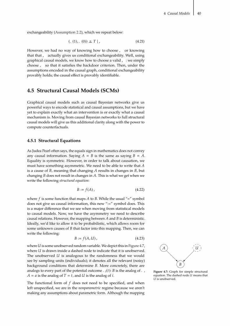
4 Causal Models 40
exchangeability (Assumption 2.2), which we repeat below:
(.(1), .(0)) ⊥⊥ ) | , (4.21)
However, we had no way of knowing how to choose , or knowing
that that, actually gives us conditional exchangeability. Well, using
graphical causal models, we know how to choose a valid, : we simply
choose , so that it satisfies the backdoor criterion. Then, under the
assumptions encoded in the causal graph, conditional exchangeability
provably holds; the causal effect is provably identifiable.
4.5 Structural Causal Models (SCMs)
Graphical causal models such as causal Bayesian networks give us
powerful ways to encode statistical and causal assumptions, but we have
yet to explain exactly what an intervention is or exactly what a causal
mechanism is. Moving from causal Bayesian networks to full structural
causal models will give us this additional clarity along with the power to
compute counterfactuals.
4.5.1 Structural Equations
As Judea Pearl often says, the equals sign in mathematics does not convey
any causal information. Saying � = � is the same as saying � = �.
Equality is symmetric. However, in order to talk about causation, we
must have something asymmetric. We need to be able to write that �
is a cause of �, meaning that changing � results in changes in �, but
changing � does not result in changes in �. This is what we get when we
write the following structural equation:
� := 5 (�) , (4.22)
where 5 is some function that maps � to �. While the usual “=” symbol
does not give us causal information, this new “:=” symbol does. This
is a major difference that we see when moving from statistical models
to causal models. Now, we have the asymmetry we need to describe
causal relations. However, the mapping between � and � is deterministic.
Ideally, we’d like to allow it to be probabilistic, which allows room for
some unknown causes of � that factor into this mapping. Then, we can
write the following:
� := 5 (�,*) , (4.23)
where* is someunobserved randomvariable.Wedepict this in Figure 4.7,
where* is drawn inside a dashed node to indicate that it is unobserved.
The unobserved * is analogous to the randomness that we would
see by sampling units (individuals); it denotes all the relevant (noisy)
background conditions that determine �. More concretely, there are
analogs to every part of the potential outcome .8(C): � is the analog of .,
� = 0 is the analog of ) = C, and* is the analog of 8.
�
� *
Figure 4.7: Graph for simple structural
equation. The dashed node* means that
* is unobserved.
The functional form of 5 does not need to be specified, and when
left unspecified, we are in the nonparametric regime because we aren’t
making any assumptions about parametric form. Although the mapping

4 Causal Models 41
7Trust me; the recursion ends. The base
case was specified.
is deterministic, because it takes a random variable * (a “noise” or
“background conditions” variable) as input, it can represent any stochastic
mapping, so structural equations generalize the probabilistic factors
%(G8 | pa8) that we’ve been using throughout this chapter. Therefore, all
the results that we’ve seen such as the truncated factorization and the
backdoor adjustment still holdwhenwe introduce structural equations.
Cause and Causal Mechanism Revisited We have now come to the
more precise definitions of what a cause is (Definition 3.2) and what a
causal mechanism is (introduced in Section 4.2). A causal mechanism
that generates a variable is the structural equation that corresponds to
that variable. For example, the causal mechanism for � is Equation 4.23.
Similarly, - is a direct cause of . if - appears on the right-hand side of
the structural equation for .. We say that - is a cause of . if - is a direct
cause of any of the causes of .7or if - is a direct cause of ..
We only showed a single structural equation in Equation 4.23, but there
can be a large collection of structural equations in a single model, which
we will commonly label". For example, we write structural equations
for Figure 4.8 below:
" :
� := 5�(�,*�)� := 5�(�, �,*�)� := 5�(�, �,*�)
(4.24)
�
� *�
�
*�
�
*�
Figure 4.8: Graph for the structural equa-
tions in Equation 4.24.
In causal graphs, the noise variables are often implicit, rather than
explicitly drawn. The variables that we write structural equations for
are known as endogenous variables. These are the variables whose causal
mechanisms we are modeling – the variables that have parents in the
causal graph. In contrast, exogenous variables are variables who do not
have any parents in the causal graph; these variables are external to our
causal model in the sense that we choose not to model their causes. For
example, in the causal model described by Figure 4.8 and Equation 4.24,
the endogenous variables are {�, �, �}. And the exogenous variables
are {�,*� , *� , *�}.
Definition 4.2 (Structural Causal Model (SCM)) A structural causalmodel is a tuple of the following sets:
1. A set of endogenous variables +2. A set of exogenous variables*3. A set of functions 5 , one to generate each endogenous variable as a
function of other variables
For example, ", the set of three equations above in Equation 4.24
constitutes an SCMwith corresponding causal graph in Figure 4.8. Every
SCM implies an associated causal graph: for each structural equation,
draw an edge from every variable on the right-hand side to the variable
on the left-hand side.
If the causal graph contains no cycles (is a DAG) and the noise variables
* are independent, then the causal model is Markovian; the distribution% is Markov with respect to the causal graph. If the causal graph doesn’t
contain cycles but the noise terms are dependent, then the model is semi-Markovian. For example, if there is unobserved confounding, the model

4 Causal Models 42
[5]: Holland (1986), ‘Statistics and Causal
Inference’
[17]: Pearl (2009), ‘Causal inference in
statistics: An overview’
is semi-Markovian. Finally, the graphs of non-Markovian models contain
cycles. We will largely be considering Markovian and semi-Markovian
models in this book.
4.5.2 Interventions
Interventions in SCMs are remarkably simple. The intervention do() = C)simply corresponds to replacing the structural equation for ) with ) := C.
For example, consider the following causal model" with corresponding
causal graph in Figure 4.9:
-
) .
Figure 4.9: Basic causal graph
" :
) := 5)(-,*)). := 5.(-, ),*.)
(4.25)
If we then intervene on ) to set it to C, we get the interventional SCM"C
below and corresponding manipulated graph in Figure 4.10.
"C :
) := C
. := 5.(-, ),*.)(4.26)
-
) .
Figure 4.10: Basic causal with the the in-
coming edges to ) removed, due to the
intervention do() = C).
The fact that do() = C) only changes the equation for ) and no other
variables is a consequence of the modularity assumption; these causal
mechanisms (structural equations) are modular. Assumption 4.1 states
the modularity assumption in the context of causal Bayesian networks,
but we need a slightly different translation of this assumption for SCMs.
Assumption 4.2 (Modularity Assumption for SCMs) Consider an SCM" and an interventional SCM"C that we get by performing the interventiondo() = C). The modularity assumption states that " and "C share all oftheir structural equations except the structural equation for ), which is ) := C
in"C .
In other words, the intervention do() = C) is localized to ). None of the
other structural equations change because they are modular; the causal
mechanisms are independent. The modularity assumption for SCMs is
what gives us what Pearl calls the The Law of Counterfactuals, which
we briefly mentioned at the end of Section 4.2, after we defined the
modularity assumption for causal Bayesian networks. But before we can
get to that, we must first introduce a bit more notation.
In the causal inference literature, there are many different ways of writing
the unit-level potential outcome. In Chapter 2, we used .8(C). However,
there are other ways such as .C8or even .C(D). For example, in his
prominent potential outcomes paper, Holland [5] uses the .C(D) notation.In this notation, D is the analog of 8, just as we mentioned is the case
for the * in Equation 4.23 and the paragraph that followed it. This is
the notation that Pearl uses for SCMs as well [see, e.g., 17, Definition
4]. So .C(D) denotes the outcome that unit D would observe if they take
treatment C, given that the SCM is ". Similarly, we define ."C (D) asthe outcome that unit D would observe if they take treatment C, given
that the SCM is"C (remember that"C is the same SCM as" but with
the structural equation for ) changed to ) := C). Now, we are ready to

4 Causal Models 43
8Active reading exercise: Can you recall
which was the other key principle/as-
sumption?
Active reading exercise: Take what you
now know about structural equations,
and relate it to other parts of this chap-
ter. For example, how do interventions in
structural equations relate to the modu-
larity assumption? How does the mod-
ularity assumption for SCMs (Assump-
tion 4.2) relate to the modularity assump-
tion in causal Bayesian networks (Assump-
tion 4.1)? Does this modularity assump-
tion for SCMs still give us the backdoor
adjustment?
,
") .
Figure 4.11: Causal graph where all cau-
sation is blocked by conditioning on".
,
") .
Figure 4.12: Causal graph where part of
the causation is blocked by conditioning
on".
,
) .
/
Figure 4.13: Causal graph where condi-
tioning on the collider / induces bias.
present one of Pearl’s two key principles from which all other causal
results follow:8
Definition 4.3 (The Law of Counterfactuals (and Interventions))
.C(D) = ."C (D) (4.27)
This is called “The Law of Counterfactuals” because it gives us informa-
tion about counterfactuals. Given an SCM with enough details about it
specified, we can actually compute counterfactuals. This is a big deal
because this is exactly what the fundamental problem of causal inference
(Section 2.2) told uswe cannot do.Wewon’t saymore about how to do this
until we get to the dedicated chapter for counterfactuals: Chapter 14.
4.5.3 Collider Bias and Why to Not Condition onDescendants of Treatment
In defining the backdoor criterion (Definition 4.1) for the backdoor
adjustment (Theorem 4.2), not only did we specify that the adjustment
set, blocks all backdoor paths, but we also specified that, does not
contain any descendants of ). Why? There are two categories of things
that could go wrong if we condition on descendants of ):
1. We block the flow of causation from ) to ..
2. We induce non-causal association between ) and ..
As we’ll see, it is fairly intuitive why we want to avoid the first category.
The second category is a bit more complex, and we’ll break it up into two
different parts, each with their own paragraph. This more complex part
is actually why we delayed this explanation to after we introduced SCMs,
rather than back when we introduced the backdoor criterion/adjustment
in Section 4.4.
If we condition on a node that is on a directed path from ) to ., then we
block the flow of causation along that causal path. We will refer to a node
on a directed path from ) to . as a mediator, as it mediates the effect of
) on .. For example, in Figure 4.11, all of the causal flow is blocked by
". This means that we will measure zero association between ) and .
(given that, blocks all backdoor paths). In Figure 4.12, only a portion of
the causal flow is blocked by". This is because causation can still flow
along the ) → . edge. In this case, we will get a non-zero estimate of
the causal effect, but it will still be biased, due to the causal flow that"
blocks.
If we condition on a descendant of) that isn’t amediator, it could unblock
a path from ) to . that was blocked by a collider. For example, this is
the case with conditioning on / in Figure 4.13. This induces non-causal
association between ) and ., which biases the estimate of the causal
effect. Consider the following general kind of path, where → · · · →denotes a directed path: ) → · · · → /← · · · ← .. Conditioning on /,
or any descendant of / in a path like this, will induce collider bias. Thatis, the causal effect estimate will be biased by the non-causal association
that we induce when we condition on / or any of its descendants (see
Section 3.6).

4 Causal Models 44
,
") .
/
Figure 4.14: Causal graph where the child
of a mediator is conditioned on.
,
*"
") .
/
Figure 4.15: Magnified causal graph
where the child of a mediator is condi-
tioned on.
/2
) .
/1/3
Figure 4.16: Causal graph depicting M-
Bias.
What about conditioning on / in Figure 4.14? Would that induce bias?
Recall that graphs are frequently drawn without explicitly drawing
the noise variables. If we magnify part of the graph, making "’s noise
variable explicit, we get Figure 4.15. Now, we see that ) → " ← *"
forms an immorality. Therefore, conditioning on / induces an association
between ) and*" . This induced non-causal association is another form
of collider bias. You might find this unsatisfying because . is not one
of the immoral parents here; rather ) and *" are the ones living the
immoral lifestyle. So why would this change the association between )
and .? One way to get the intuition for this is that there is now induced
association flowing between ) and*" through the edge ) → ", which
is also an edge that causal association is flowing along. You can think of
these two types of association getting tangled up along the ) → " edge,
making the observed association between ) and . not purely causal. See
Pearl [18, Section 11.3.1 and 11.3.3] for more information on this topic.
Note that we actually can condition on some descendants of ) without
inducing non-causal associations between ) and .. For example, condi-
tioning on descendants of ) that aren’t on any causal paths to . won’t
induce bias. However, as you can see from the above paragraph, this can
get a bit tricky, so it is safest to just not condition on any descendants of
), as the backdoor criterion prescribes. Even outside of graphical causal
models (e.g. in potential outcomes literature), this rule is often applied; it
is usually described as not conditioning on any post-treatment covariates.
M-Bias Unfortunately, even if we only condition on pretreatment co-
variates, we can still induce collider bias. Consider what would happen
if we condition on the collider /2 in Figure 4.16. Doing this opens up
a backdoor path, along which non-causal association can flow. This is
known as M-bias due to the M shape that this non-causal association
flows along when the graph is drawn with children below their parents.
For many examples of collider bias, see Elwert and Winship [19].
4.6 Example Applications of the BackdoorAdjustment
4.6.1 Association vs. Causation in a Toy Example
In this section, we posit a toy generative process and derive the bias of the
associational quantity E[. | C]. We compare this to the causal quantity
E[. | do(C)], which gives us exactly what we want. Note that both of
these quantities are actually functions of C. If the treatment were binary,
then we would just look at the difference between the quantities with
) = 1 and with ) = 0. However, because our generative processes will be
linear,3 E[. |C]3C and
3 E[. |do(C)]3C actually gives us all the information about
the treatment effect, regardless of if treatment is continuous, binary, or
multi-valued. We will assume infinite data so that we can work with
expectations. This means this section has nothing to do with estimation;
for estimation, see the next section
The generative process thatwe consider has the causal graph in Figure 4.17
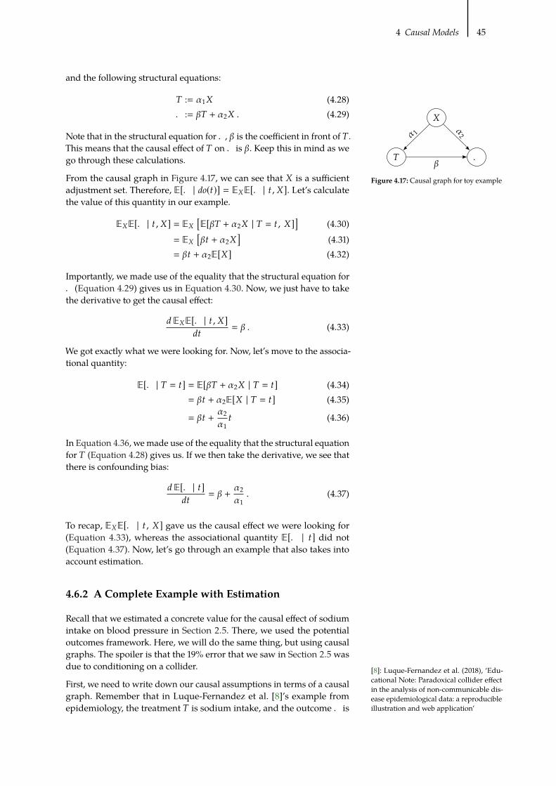
4 Causal Models 45
[8]: Luque-Fernandez et al. (2018), ‘Edu-
cational Note: Paradoxical collider effect
in the analysis of non-communicable dis-
ease epidemiological data: a reproducible
illustration and web application’
and the following structural equations:
) := 1- (4.28)
. := �) + 2- . (4.29)
Note that in the structural equation for ., � is the coefficient in front of ).
This means that the causal effect of ) on . is �. Keep this in mind as we
go through these calculations.
-
) .
1 2
�
Figure 4.17: Causal graph for toy exampleFrom the causal graph in Figure 4.17, we can see that - is a sufficient
adjustment set. Therefore, E[. | do(C)] = E-E[. | C , -]. Let’s calculatethe value of this quantity in our example.
E-E[. | C , -] = E-[E[�) + 2- | ) = C , -]
](4.30)
= E-[�C + 2-
](4.31)
= �C + 2E[-] (4.32)
Importantly, we made use of the equality that the structural equation for
. (Equation 4.29) gives us in Equation 4.30. Now, we just have to take
the derivative to get the causal effect:
3 E-E[. | C , -]3C
= � . (4.33)
We got exactly what we were looking for. Now, let’s move to the associa-
tional quantity:
E[. | ) = C] = E[�) + 2- | ) = C] (4.34)
= �C + 2E[- | ) = C] (4.35)
= �C + 2
1
C (4.36)
In Equation 4.36, we made use of the equality that the structural equation
for ) (Equation 4.28) gives us. If we then take the derivative, we see that
there is confounding bias:
3 E[. | C]3C
= � + 2
1
. (4.37)
To recap, E-E[. | C , -] gave us the causal effect we were looking for
(Equation 4.33), whereas the associational quantity E[. | C] did not
(Equation 4.37). Now, let’s go through an example that also takes into
account estimation.
4.6.2 A Complete Example with Estimation
Recall that we estimated a concrete value for the causal effect of sodium
intake on blood pressure in Section 2.5. There, we used the potential
outcomes framework. Here, we will do the same thing, but using causal
graphs. The spoiler is that the 19% error that we saw in Section 2.5 was
due to conditioning on a collider.
First, we need to write down our causal assumptions in terms of a causal
graph. Remember that in Luque-Fernandez et al. [8]’s example from
epidemiology, the treatment ) is sodium intake, and the outcome . is

4 Causal Models 46
blood pressure. The covariates are age, and amount of protein in urine
(proteinuria) /. Age is a common cause of both blood pressure and the
body’s ability to self-regulate sodium levels. In contrast, high amounts
of urinary protein are caused by high blood pressure and high sodium
intake. This means that proteinuria is a collider. We depict this causal
graph in Figure 4.18.
,
) .
/
Figure 4.18: Causal graph for the blood
pressure example. ) is sodium intake. .is blood pressure., is age. And, impor-
tantly, the amount of protein excreted in
urine / is a collider.
Because / is a collider, conditioning on it induces bias. Because, and /
were grouped together as “covariates” - in Section 2.5, we conditioned
on all of them. This is why we saw that our estimate was 19% off from
the true causal effect 1.05. Now that we’ve made the causal relationships
clear with a causal graph, the backdoor criterion (Definition 4.1) tells us
to only adjust for, and to not adjust for /. More precisely, we were
doing the following adjustment in Section 2.5:
E,,/E[. | C , ,, /] (4.38)
And now, we will use the backdoor adjustment (Theorem 4.2) to change
our statistical estimand to the following:
E,E[. | C , ,] (4.39)
We have simply removed the collider / from the variables we adjust for.
For estimation, just as we did in Section 2.5, we use a model-assisted
estimator. We replace the outer expectation over, with an empirical
mean over, and replace the conditional expectation E[. | C , ,]with a
machine learning model (in this case, linear regression).
Just as writing down the graph has lead us to simply not condition on /
in Equation 4.39, the code for estimation also barely changes. We need to
change just a single line of code in our previous program (Listing 2.1).
We display the full program with the fixed line of code below:
Listing 4.1: Python code for estimating the
ATE, without adjusting for the collider
1 import numpy as np
2 import pandas as pd
3 from sklearn.linear_model import LinearRegression
4
5 Xt = df[['sodium', 'age']]
6 y = df['blood_pressure']
7 model = LinearRegression()
8 model.fit(Xt, y)
9
10 Xt1 = pd.DataFrame.copy(Xt)
11 Xt1['sodium'] = 1
12 Xt0 = pd.DataFrame.copy(Xt)
13 Xt0['sodium'] = 0
14 ate_est = np.mean(model.predict(Xt1) - model.predict(Xt0))
15 print('ATE estimate:', ate_est)
Full code, complete with simulation,
is available at https://github.com/
bradyneal/causal-book-code/blob/
master/sodium_example.py.
Namely, we’ve changed line 5 from
5 Xt = df[['sodium', 'age', 'proteinuria']]
in Listing 2.1 to
5 Xt = df[['sodium', 'age']]
in Listing 4.1. When we run this revised code, we get an ATE estimate of
1.0502, which corresponds to 0.02% error (true value is 1.05) when using

4 Causal Models 47
9Active reading exercise: Given that . is
generated as a linear function of ) and, ,
could we have just used the coefficient in
front of ) in the linear regression as an
estimate for the causal effect?
/2
) .
/1/3
Figure 4.19: Causal graph depicting M-
Bias that can only be avoided by not con-
ditioning on the collider /2. This is due to
the fact that the dashed nodes /1 and /3
are unobserved.
[20]:Galles andPearl (1998), ‘AnAxiomatic
Characterization of Causal Counterfactu-
als’
[21]: Halpern (1998), ‘Axiomatizing Causal
Reasoning’
[18]: Pearl (2009), Causality
[13]: Koller and Friedman (2009), Proba-bilistic Graphical Models: Principles and Tech-niques
a fairly large sample.9
Progression of Reducing Bias When looking at the total association
between) and. by simply regressing. on), we got an estimate that was
a staggering 407% off of the true causal effect, due largely to confounding
bias (see Section 2.5). When we adjusted for all covariates in Section 2.5,
we reduced the percent error all the way down to 19%. In this section,
we saw this remaining error is due to collider bias. When we removed
the collider bias, by not conditioning on the collider /, the error became
non-existent.
Potential Outcomes and M-Bias In fairness to the general culture
around the potential outcomes framework, it is common to only condition
on pretreatment covariates. This would prevent a practitioner who
adheres to this rule from conditioning on the collider / in Figure 4.18.
However, there is no reason that there can’t be pretreatment colliders
that induce M-bias (Section 4.5.3). In Figure 4.19, we depict an example
of M-bias that is created by conditioning on /2. We could fix this by
additionally conditioning on /1 and/or /3, but in this example, they are
unobserved (indicated by the dashed lines). This means that the only
way to avoid M-bias in Figure 4.19 is to not condition on the covariates
/2.
4.7 Assumptions Revisited
The first main set of assumptions is encoded by the causal graph that we
write down. Exactly what this causal graph means is determined by two
main assumptions, each of which can take on several different forms:
1. The Modularity AssumptionDifferent forms:
I ModularityAssumption forCausal BayesianNetworks (Assumption 4.1)
I Modularity Assumption for SCMs (Assumption 4.2)
I The Law of Counterfactuals (Definition 4.3)
2. The Markov AssumptionDifferent equivalent forms:
I Local Markov assumption (Assumption 3.1)
I Bayesian network factorization (Definition 3.1)
I Global Markov assumption (Theorem 3.1)
Given, these two assumptions (and positivity), if the backdoor criterion
(Definition 4.1) is satisfied in our assumed causal graph, then we have
identification. Note that although the backdoor criterion is a sufficient
condition for identification, it is not a necessary condition. We will see
this more in Chapter 6.
Now that you’re familiar with causal
graphical models and SCMs, it may be
worth going back and rereading Chap-
ter 2 while trying to make connections
to what you’ve learned about graphical
causal models in these past two chapters.
More Formal If you’re really into fancy formalism, there are some
relevant sources to check out. You can see the fundamental axioms that
underlie The Law of Counterfactuals in [20, 21], or if you want a textbook,
you can find them in [18, Chapter 7.3]. To see proofs of the equivalence of
all three forms of the Markov assumption, see, for example, [13, Chapter
3].

4 Causal Models 48
[22]: Ogburn and VanderWeele (2014),
‘Causal Diagrams for Interference’
[18]: Pearl (2009), Causality
[23]: Pearl (2010), ‘On the consistency rule
in causal inference: axiom, definition, as-
sumption, or theorem?’
Connections to No Interference, Consistency, and Positivity The no
interference assumption (Assumption 2.4) is commonly implicit in causal
graphs, since the outcome . (think .8) usually only has a single node )
(think)8) for treatment as a parent, rather than havingmultiple treatment
nodes)8 ,)8−1,)8+1, etc. as parents. However, causal DAGs can be extended
to settings where there is interference [22]. Consistency (Assumption 2.5)
follows from the axioms of SCMs (see [18, Corollary 7.3.2] and [23]).
Positivity (Assumption 2.3) is still a very important assumption that we
must make, though it is sometimes neglected in the graphical models
literature.

The symbol
3= means “equal in distribu-
tion.”
Randomized Experiments 55.1 Comparability and Covari-
ate Balance . . . . . . . . . . 495.2 Exchangeability . . . . . . . 505.3 No Backdoor Paths . . . . . 51
Randomized experiments are noticeably different from observational
studies. In randomized experiments, the experimenter has complete con-
trol over the treatment assignment mechanism (how treatment is assigned).
For example, in the most simple kind of randomized experiment, the
experimenter randomly assigns (e.g. via coin toss) each participant to
either the treatment group or the control group. This complete control
over how treatment is chosen is what distinguishes randomized experi-
ments from observational studies. In this simple experimental setup, the
treatment isn’t a function of covariates at all! In contrast, in observational
studies, the treatment is almost always a function of some covariate(s).
As we will see, this difference is key to whether or not confounding is
present in our data.
In randomized experiments, association is causation. This is because ran-domized experiments are special in that they guarantee that there is no
confounding.As a consequence, this allows us tomeasure the causal effect
E[.(1)]−E[.(0)]via the associational differenceE[. | ) = 1] − E[. | ) = 0].In the following sections, we explain why this is the case from a variety
of different perspectives. If any one of these explanations clicks with you,
that might be good enough. Definitely stick through to the most visually
appealing explanation in Section 5.3.
5.1 Comparability and Covariate Balance
Ideally, the treatment and control groups would be the same, in all
aspects, except for treatment. This would mean they only differ in the
treatment they receive (i.e. they are comparable). This would allow us to
attribute any difference in the outcomes of the treatment and control
groups to the treatment. Saying that these treatment groups are the same
in everything other than their treatment and outcomes is the same as
saying they have the same distribution of confounders. Because people
often check for this property on observed variables (often what people
mean by “covariates”), this concept is known as covariate balance.
Definition 5.1 (Covariate Balance) We have covariate balance if the distri-bution of covariates - is the same across treatment groups. More formally,
%(- | ) = 1) 3=%(- | ) = 0) (5.1)
Randomization implies covariate balance, across all covariates, even
unobserved ones. Intuitively, this is because the treatment is chosen at
random, regardless of -, so the treatment and control groups should
look very similar. The proof is simple. Because ) is not at all determined
by - (solely by a coin flip), ) is independent of -. This means that

5 Randomized Experiments 50
1Recall that the intuition is that covariate
balance means that everything is the same
between the treatment groups, except for
the treatment, so the treatment must be
the explanation for the change in ..
%(- | ) = 1) 3=%(-). Similarly, it means %(- | ) = 0) 3=%(-). Therefore,we have %(- | ) = 1) 3=%(- | ) = 0).
Although we have proven that randomization implies covariate balance,
we have not proven that that covariate balance implies that association is
causation.1We’ll now prove that by showing that %(H | do(C)) = %(H | C).
For the proof, the main property we utilize is that covariate balance
implies - and ) are independent.
Proof. First, let - be a sufficient adjustment set that potentially contains
unobserved variables (randomization also balances unobserved covariates).
Such an adjustment set must exist because we allow it to contain any
variables, observed or unobserved. Then, we have the following from the
backdoor adjustment (Theorem 4.2):
%(H | do(C)) =∑G
%(H | C , G)%(G) (5.2)
By multiplying by%(C |G)%(C |G) , we get the joint distribution in the numerator:
=∑G
%(H | C , G)%(C | G)%(G)%(C | G) (5.3)
=∑G
%(H, C, G)%(C | G) (5.4)
Now, we use the important property that - ⊥⊥ ):
=∑G
%(H, C, G)%(C) (5.5)
An application of Bayes rule and marginalization gives us the rest:
=∑G
%(H, G | C) (5.6)
= %(H | C) (5.7)
5.2 Exchangeability
Exchangeability (Assumption 2.1) gives us another perspective on why
randomizationmakes causation equal to association. To seewhy, consider
the following thought experiment. We decide an individual’s treatment
group using a random coin flip as follows: if the coin is heads, we assign
the individual to the treatment group () = 1), and if the coins is tails,
we assign the individual to the control group () = 0). If the groups are
exchangeable, we could exchange these groups, and the average outcomes
would remain the same. This is intuitively true if we chose the groups
with a coin flip. Imagine simply swapping the meaning of “heads” and
“tails” in this experiment. Would you expect that to change the results at
all? No. This is why randomized experiments give us exchangeability.

5 Randomized Experiments 51
Recall from Section 2.3.2 that mean exchangeability is formally the
following:
E[.(1) | ) = 1] = E[.(1) | ) = 0] (5.8)
E[.(0) | ) = 0] = E[.(0) | ) = 1] (5.9)
The “exchange” is when we go from .(1) in the treatment group to .(1)in the control group (Equation 5.8) and from .(0) in the control group to
.(0) in the treatment group (Equation 5.9).
To see the proof of why association is causation in randomized ex-
periments through the lens of exchangeability, recall the proof from
Section 2.3.2. First, recall that Equation 5.8 means that both quantities in
it are equal to the marginal expected outcome E[.(1)] and, similarly, that
Equation 5.8 means that both quantities in it are equal to the marginal
expected outcome E[.(0)]. Then, we have the following proof:
E[.(1)] − E[.(0)] = E[.(1) | ) = 1] − E[.(0) | ) = 0] (2.3 revisited)
= E[. | ) = 1] − E[. | ) = 0] (2.4 revisited)
5.3 No Backdoor Paths
The final perspective that we’ll look at to see why association is causation
in randomized experiments is that of graphical causal models. In regular
observational data, there is almost always confounding. For example,
in Figure 5.1, we see that - is a confounder of the effect of ) on ..
Non-causal association flows along the backdoor path ) ← - → ..
-
) .
confounding association
Figure 5.1: Causal structure of - con-
founding the effect of ) on ..
However, if we randomize ), something magical happens: ) no longer
has any causal parents, as we depict in Figure 5.2. This is because ) is
purely random. It doesn’t depend on anything other than the output of a
coin toss (or a quantum random number generator, if you’re into the kind
of stuff). Because ) has no incoming edges, under randomization, there
are no backdoor paths. So the empty set is a sufficient adjustment set. This
means that all of the association that flows from ) to . is causal. We can
identify %(. | do() = C)) by simply applying the backdoor adjustment
(Theorem 4.2), adjusting for the empty set:
%(. | do() = C)) = %(. | ) = C)
-
) .
Figure 5.2: Causal structure when we ran-
domize treatment.
With that, we conclude our discussion of why association is causation in
randomized experiments. Hopefully, at least one of these three explana-
tions is intuitive to you and easy to store in long-term memory.

Nonparametric Identification 66.1 Frontdoor Adjustment . . . 526.2 do-calculus . . . . . . . . . . 55
Application: Frontdoor Ad-justment . . . . . . . . . . . 57
6.3 Determining Identifiabilityfrom the Graph . . . . . . . 58
In Section 4.4, we saw that satisfying the backdoor criterion is sufficient
to give us identifiability, but is the backdoor criterion also necessary?
In other words, is it possible to get identifiability without being able to
block all backdoor paths?
As an example, consider that we have data generated according to the
graph in Figure 6.1. We don’t observe, in this data, so we can’t block the
backdoor path through, and the confounding association that flows
along it. But we still need to identify the causal effect. It turns out that it
is possible to identify the causal effect in this graph, using the frontdoor
criterion. We’ll see the frontdoor criterion and corresponding adjustment
in Section 6.1. Then, we’ll consider even more general identification in
Section 6.2 when we introduce do-calculus. We’ll conclude with graphical
conditions for identifiability in Section 6.3.
,
") .
confounding association
causal association
Figure 6.1: Causal graph where, is un-
observed, so we cannot block the back-
door path. We depict the flow of causal
association and the flow of confounding
association with dashed lines.
6.1 Frontdoor Adjustment
The high-level intuition for why we can identify the causal effect of ) on
. in the graph in Figure 6.1 (evenwhenwe can’t adjust for the confounder
, because it is unobserved) is as follows: a mediator like " is very
helpful; we can isolate the association that flows through" by focusing
our statistical analysis on", and the only association that flows through
" is causal association (association flowing along directed paths from )
to .). We illustrate this intuition in Figure 6.2, where we depict only the
causal association. In this section, we will focus our analysis on" using a
three step procedure (see Figure 6.3 for our corresponding illustration):
1. Identify the causal effect of ) on".
2. Identify the causal effect of" on ..
3. Combine the above steps to identify the causal effect of ) on ..
,
") .
focus
only causal association
Figure 6.2: In contrast to Figure 6.1, when
we focus our analysis on ", we are able
to isolate only the causal association.
,
") .Step 1 Step 2
Step 3
Figure 6.3: Illustration of steps to get to
the frontdoor adjustment.
Step 1 First, we will identify the effect of ) on": %(< | do(C)). Because. is a collider on the ) −" path through, , it blocks that backdoor path.
So there are no unblocked backdoor paths from ) to". This means that
the only association that flows from ) to" is the causal association that
flows along the edge connecting them. Therefore, we have the following
identification via the backdoor adjustment (Theorem 4.2, using the empty
set as the adjustment set):1
1Active reading exercise: Write a proof for
Equation 6.1 without using the backdoor
adjustment. Instead, start from the trun-
cated factorization (Proposition 4.1) like
we did in Section 4.3.1. Hint: The proof
can be quite short. We provide a proof in
Appendix A.1, in case you get stuck.
%(< | do(C)) = %(< | C) (6.1)
Step 2 Second, we will identify the effect of " on .: %(H | do(<)).Because ) blocks the backdoor path" ← ) ←, → ., we can simply
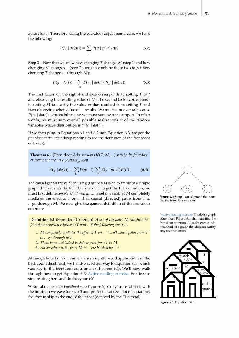
6 Nonparametric Identification 53
equation
quick
maths
,
)
"
.much
rigor
very
wow
Figure 6.5: Equationtown
adjust for ). Therefore, using the backdoor adjustment again, we have
the following:
%(H | do(<)) =∑C
%(H | <, C)%(C) (6.2)
Step 3 Now that we know how changing ) changes" (step 1) and how
changing " changes . (step 2), we can combine these two to get how
changing ) changes . (through"):
%(H | do(C)) =∑<
%(< | do(C))%(H | do(<)) (6.3)
The first factor on the right-hand side corresponds to setting ) to C
and observing the resulting value of". The second factor corresponds
to setting " to exactly the value < that resulted from setting ) and
then observing what value of . results. We must sum over < because
%(< | do(C)) is probabilistic, so we must sum over its support. In other
words, we must sum over all possible realizations < of the random
variables whose distribution is %(" | do(C)).
If we then plug in Equations 6.1 and 6.2 into Equation 6.3, we get the
frontdoor adjustment (keep reading to see the definition of the frontdoor
criterion):
Theorem 6.1 (Frontdoor Adjustment) If (), ",.) satisfy the frontdoorcriterion and we have positivity, then
%(H | do(C)) =∑<
%(< | C)∑C′%(H | <, C′)%(C′) (6.4)
The causal graph we’ve been using (Figure 6.4) is an example of a simple
graph that satisfies the frontdoor criterion. To get the full definition, we
must first define complete/full mediation: a set of variables" completely
mediates the effect of ) on . if all causal (directed) paths from ) to
. go through ". We now give the general definition of the frontdoor
criterion:
,
") .
Figure 6.4: Simple causal graph that satis-
fies the frontdoor criterion
Definition 6.1 (Frontdoor Criterion) A set of variables " satisfies thefrontdoor criterion relative to ) and . if the following are true:
1. " completely mediates the effect of ) on . (i.e. all causal paths from )
to . go through").2. There is no unblocked backdoor path from ) to".3. All backdoor paths from" to . are blocked by ).2
2Active reading exercise: Think of a graph
other than Figure 6.4 that satisfies the
frontdoor criterion. Also, for each condi-
tion, think of a graph that does not satisfyonly that condition.
Although Equations 6.1 and 6.2 are straightforward applications of the
backdoor adjustment, we hand-waved our way to Equation 6.3, which
was key to the frontdoor adjustment (Theorem 6.1). We’ll now walk
through how to get Equation 6.3. Active reading exercise: Feel free to
stop reading here and do this yourself.
We are about to enter Equationtown (Figure 6.5), so if you are satisfiedwith
the intuition we gave for step 3 and prefer to not see a lot of equations,
feel free to skip to the end of the proof (denoted by the symbol).

6 Nonparametric Identification 54
3Active reading exercise: Why would it
be easy to marginalize out F if it were
the case that %(F) = %(F | <)? And why
does this equality not hold?
,
") .
Figure 6.6: Simple causal graph that satis-
fies the frontdoor criterion
4Active reading exercise: Why is
%(H | F, <) equal to %(H | F, C′, <)?
Proof. As usual, we start with the truncated factorization, using the
causal graph in Figure 6.4. From the Bayesian network factorization
(Definition 3.1), we have the following:
%(F, C, <, H) = %(F)%(C | F)%(< | C)%(H | F, <) (6.5)
Then, using the truncated factorization (Proposition 4.1), we remove the
factor for ):
%(F, <, H | do(C)) = %(F)%(< | C)%(H | F, <) (6.6)
Next, we marginalize out F and <:∑<
∑F
%(F, <, H | do(C)) =∑<
∑F
%(F)%(< | C)%(H | F, <) (6.7)
%(H | do(C)) =∑<
%(< | C)∑F
%(H | F, <)%(F) (6.8)
Even though we’ve removed all the do operators, recall that we are not
done because, is unobserved. So we must also remove the F from the
expression. This is where we have to get a bit creative.
We want to be able to combine %(H | F, <) and %(F) into a joint factor
over both H and F so that we can marginalize out F. To do this, we
need to get < behind the conditioning bar of the %(F) factor. This would
be easy if we could just swap %(F) out for %(F | <) in Equation 6.8.3
The key thing to notice is that we actually can include < behind the
conditioning bar if C were also there because ) d-separates, from" in
Figure 6.6. In math, this means that the following equality holds:
%(F | C) = %(F | C , <) (6.9)
Great, so how do we get C into this party? The usual trick of conditioning
on it and marginalizing it out:
%(H | do(C)) =∑<
%(< | C)∑F
%(H | F, <)%(F) (6.8 revisited)
=∑<
%(< | C)∑F
%(H | F, <)∑C′%(F | C′)%(C′) (6.10)
=∑<
%(< | C)∑F
%(H | F, <)∑C′%(F | C′, <)%(C′) (6.11)
=∑<
%(< | C)∑C′%(C′)
∑F
%(H | F, <)%(F | C′, <) (6.12)
Great, but now we can’t combine %(H | F, <) and %(F | C′, <) because%(H | F, <) is missing this newly introduced C′ behind its conditioning
bar. Luckily, we can fix that4and combine the two factors:
=∑<
%(< | C)∑C′%(C′)
∑F
%(H | F, <)%(F | C′, <) (6.13)
=∑<
%(< | C)∑C′%(C′)
∑F
%(H | F, C′, <)%(F | C′, <)
(6.14)
=∑<
%(< | C)∑C′%(C′)
∑F
%(H, F | C′, <) (6.15)
=∑<
%(< | C)∑C′%(C′)%(H | C′, <) (6.16)

6 Nonparametric Identification 55
[24]: Pearl (1995), ‘Causal diagrams for
empirical research’
This matches the result stated in Theorem 6.1, so we’ve completed the
derivation of the frontdoor adjustment without using the backdoor
adjustment. However, we still need to show that Equation 6.3 is correct
to justify step 3. To do that, all that’s left is to recognize that these parts
match Equations 6.1 and 6.2 and plug those in:
=∑<
%(< | do(C))%(H | do(<)) (6.17)
%(< | do(C)) = %(< | C) (6.1)
%(H | do(<)) =∑C
%(H | <, C)%(C) (6.2)
And we’re done! We just needed to be a bit clever with our uses of d-
separation and marginalization. Part of why we went through that proof
is because we will prove the frontdoor adjustment using do-calculus inSection 6.2. This way you can easily compare a proof using the truncated
factorization to a proof using do-calculus to prove the same result.
6.2 do-calculus
As we saw in the last section, it turns out that satisfying the backdoor
criterion (Definition 4.1) isn’t necessary to identify causal effects. For
example, if the frontdoor criterion (Definition 6.1) is satisfied, that also
gives us identifiability. This leads to the following questions: can we
identify causal estimands when the associated causal graph satisfies
neither the backdoor criterion nor the frontdoor criterion? If so, how?
Pearl’s do-calculus [24] gives us the answer to these questions.
As we will see, the do-calculus gives us tools to identify causal effects
using the causal assumptions encoded in the causal graph. It will allow
us to identify any causal estimand that is identifiable. More concretely,
consider an arbitrary causal estimand %(. | do() = C), - = G), where .
is an arbitrary set of outcome variables, ) is an arbitrary set of treatment
variables, and - is an arbitrary (potentially empty) set of covariates that
we want to choose how specific the causal effect we’re looking at is. Note
that this means we can use do-calculus to identify causal effects where
there are multiple treatments and/or multiple outcomes.
In order to present the rules of do-calculus, we must define a bit of
notation for augmented versions of the causal graph �. Let �-denote
the graph that we get if we take � and remove all of the incoming edgesto nodes in the set -; recall from Section 4.2 that this is known as the
manipulated graph. Let �- denote the graph that we get if we take � and
remove all of the outgoing edges from nodes in the set - . The mnemonic
meaning to help you remember this is to think of parents as drawn above
their children in the graph, so the bar above - is cutting its incoming
edges and the bar below- is cutting its outgoing edges. Combining these
two, we’ll use �-/
to denote the graph with the incoming edges to -
and the outgoing edges from / removed. And recall from Section 3.7 that
we use ⊥⊥� to denote d-separation in �. We’re now ready; do-calculusconsists of just three rules:
Theorem 6.2 (Rules of do-calculus) Given a causal graph �, an associated

6 Nonparametric Identification 56
[24]: Pearl (1995), ‘Causal diagrams for
empirical research’
distribution %, and disjoint sets of variables ., ), /, and, , the followingrules hold.
Rule 1:
%(H | do(C), I, F) = %(H | do(C), F) if . ⊥⊥�)/ | ),, (6.18)
Rule 2:
%(H | do(C), do(I), F) = %(H | do(C), I, F) if . ⊥⊥�),// | ),,
(6.19)
Rule 3:
%(H | do(C), do(I), F) = %(H | do(C), F) if . ⊥⊥�),/(,)
/ | ),,(6.20)
where /(,) denotes the set of nodes of / that aren’t ancestors of any node of, in �
).
Now, rather than recreate the proofs for these rules from Pearl [24], we’ll
give intuition for each of them in terms of concepts we’ve already seen in
this book.
Rule 1 Intuition If we take Rule 1 and simply remove the intervention
do(C), we get the following (Active reading exercise: what familiar concept
is this?):
%(H | I, F) = %(H | F) if . ⊥⊥� / | , (6.21)
This is just what d-separation gives us under the Markov assumption;
recall fromTheorem 3.1 that d-separation in the graph implies conditional
independence in %. This means that Rule 1 is simply a generalization of
Theorem 3.1 to interventional distributions.
Rule 2 Intuition Just as with Rule 1, we’ll remove the intervention do(C)from Rule 2 and see what this reminds us of (Active reading exercise:
what concept does this remind you of?):
%(H | do(I), F) = %(H | I, F) if . ⊥⊥�/ / | , (6.22)
This is exactly what we do when we justify the backdoor adjustment
(Theorem 4.2) using the backdoor criterion (Definition 4.1). As we saw
at the ends of Section 3.8 and Section 4.4. Association is causation if the
outcome . and the treatment / are d-separated by some set of variables
that are conditioned on, . So rule 2 is a generalization of the backdoor
adjustment to interventional distributions.
Rule 3 Intuition This is the trickiest rule to understand. Just as with
the other two rules, we’ll first remove the intervention do(C) to make
thinking about this simpler:
%(H | do(I), F) = %(H | F) if . ⊥⊥�/(,)
/ | , (6.23)
To get the equality in this equation, it must be the case that removing
the intervention do(I) (which is like taking the manipulated graph and
reintroducing the edges going into /) introduces no new association
that can affect .. Because do(I) removes the incoming edges to / to give
us �/, the main association that we need to worry about is association
flowing from / to . in �/(causal association). Therefore, you might

6 Nonparametric Identification 57
[25]: Shpitser and Pearl (2006), ‘Identifica-
tion of Joint Interventional Distributions
in Recursive Semi-MarkovianCausalMod-
els’
[26]: Huang and Valtorta (2006), ‘Pearl’s
Calculus of Intervention is Complete’
,
") .
Figure 6.7: Simple causal graph that satis-
fies the frontdoor criterion
expect that the condition that gives us the equality in Equation 6.23 is
. ⊥⊥�// | , . However, we have to refine this a bit to prevent inducing
association by conditioning on the descendants of colliders (recall from
Section 3.6). Namely, / could contain colliders in �, and, could contain
descendants of these colliders. Therefore, to not induce new association
through colliders in / when we reintroduce the incoming edges to / to
get �, we must limit the set of manipulated nodes to those that are not
ancestors of nodes in the conditioning set, : /(,).
Completeness ofdo-calculus Maybe there could exist causal estimands
that are identifiable but that can’t be identified using only the rules of
do-calculus in Theorem 6.2. Fortunately, Shpitser and Pearl [25] and
Huang and Valtorta [26] independently proved that this is not the case.
They proved that do-calculus is complete, which means that these three
rules are sufficient to identify all identifiable causal estimands. Because
these proofs are constructive, they also admit algorithms that identify
any causal estimand in polynomial time.
Nonparametric Identification Note that all of this is about nonparamet-ric identification; in other words, do-calculus tells us if we can identify
a given causal estimand using only the causal assumptions encoded
in the causal graph. If we introduce more assumptions about the dis-
tribution (e.g. linearity), we can identify more causal estimands. That
would be known as parametric identification. We don’t discuss parametric
identification in this chapter, though we will in later chapters.
6.2.1 Application: Frontdoor Adjustment
Recall the simple graph we used that satisfies the frontdoor criterion
(Figure 6.7), and recall the frontdoor adjustment:
%(H | do(C)) =∑<
%(< | C)∑C′%(H | <, C′)%(C′) (6.4 revisited)
At the end of Section 6.1, we saw a proof for the frontdoor adjustment
using just the truncated factorization. To get an idea for how do-calculusworks and the intuition we use in proofs that use it, we’ll now do the
frontdoor adjustment proof using the rules of do-calculus.
Proof. Our goal is to identify %(H | do(C)). Because we have the intu-
ition we described in Section 6.1 that the full mediator " will help us
out, the first thing we’ll do is introduce " into the equation via the
marginalization trick:
%(H | do(C)) =∑<
%(H | do(C), <)%(< | do(C)) (6.24)
Because the backdoor path from ) to" in Figure 6.7 is blocked by the
collider ., all of the association that flows from ) to" is causal, so we
can apply Rule 2 to get the following:
=∑<
%(H | do(C), <)%(< | C) (6.25)
Now, because " is a full mediator of the causal effect of ) on ., we
should be able to replace %(H | do(C), <)with %(H | do(<)), but this will

6 Nonparametric Identification 58
,
") .
Figure 6.10: �
Active reading exercise: Assuming the
backdoor criterion, prove the backdoor
adjustment using the rules of do-calculus.
take two steps of do-calculus. To remove do(C), we’ll need to use Rule 3,
which requires that) have no causal effect on. in the relevant graph. We
can get to a graph like that by removing the edge from) to" (Figure 6.9);
in do-calculus, we do this by using Rule 2 (in the opposite direction as
before) to do(<). We can do this because the existing do(C) makes it so
there are no backdoor paths from" to . in �)(Figure 6.8).
,
") .
Figure 6.8: �)
,
") .
Figure 6.9: �"
=∑<
%(H | do(C), do(<))%(< | C) (6.26)
Now, as we planned, we can remove the do(C) using Rule 3. We can use
Rule 3 here because there is no causation flowing from ) to . in �"
(Figure 6.9).
=∑<
%(H | do(<))%(< | C) (6.27)
All that’s left is to remove this last do-operator. As we discussed in
Section 6.1, ) blocks the only backdoor path from " to . in the graph
(Figure 6.10). This means, that if we can condition on ), we can get rid
of this last do-operator. As usual, we do that by conditioning on and
marginalizingout). Rearranging abit andusing C′ for themarginalization
since C is already present:
=∑<
%(< | C)∑C′%(H | do(<), C′)%(C′ | do(<))
(6.28)
Now, we can simply apply Rule 2, since ) blocks the backdoor path from
" to .:
=∑<
%(< | C)∑C′%(H | <, C′)%(C′ | do(<))
(6.29)
And finally, we can apply Rule 3 to remove the last do(<) because thereis no causal effect of" on ) (i.e. there is no directed path from" to )
in the graph in (Figure 6.10).
=∑<
%(< | C)∑C′%(H | <, C′)%(C′) (6.30)
That concludes our proof of the frontdoor adjustment using do-calculus.It follows a different path than the proof we gave at the end of Section 6.1,
where we used the truncated factorization, but both proofs rely heavily
on intuition we get from looking at the graph.
6.3 Determining Identifiability from the Graph
It’s nice to know that we can identify any causal estimand that is possible
to identify using do-calculus, but this isn’t as satisfying as knowing
whether a causal estimand is identifiable by simply looking at the causal
graph. For example, the backdoor criterion (Definition 4.1) and the
frontdoor criterion (Definition 6.1) gave us simple ways to know for
sure that a causal estimand is identifiable. However, there are plenty of

6 Nonparametric Identification 59
[27]: Tian and Pearl (2002), ‘A General
Identification Condition for Causal Effects’
5This is analogous to what we saw
with the frontdoor criterion in Section 6.1,
where we could isolate the causal associa-
tion flowing through the full mediator"
if the ) −" relationship is unconfounded
(no unblocked backdoor paths).
,2
,1,3
) .
Figure 6.11: Graph where blocking one
backdoor path unblocks another
[18]: Pearl (2009), Causality
causal estimands that are identifiable, even though the corresponding
causal graphs don’t satisfy the backdoor or frontdoor criterion. More
general graphical criteria exist that will tell us that these estimands are
identifiable. We will discuss these more general graphical criteria for
identifiability in this section.
Single Variable Intervention When we care about causal effects of
an intervention on a single variable, Tian and Pearl [27] provide a
relatively simple graphical criterion that is sufficient for identifiability:
the unconfounded children criterion.
Definition 6.2 (Unconfounded Children Criterion) This criterion issatisfied if it is possible to block all backdoor paths from the treatment variable) to all of its children that are ancestors of . with a single conditioning set.
This criterion generalizes the backdoor criterion (Definition 4.1) and the
frontdoor criterion (Definition 6.1). Like them, it is a sufficient conditionfor identifiability:
Theorem 6.3 (Unconfounded Children Identifiability) Let . be the setof outcome variables and ) be a single variable. If the unconfounded childrencriterion and positivity are satisfied, then %(. = H | do() = C)) is identifiable[27].
The intuition for unconfounded children criterion implies identifiability
is similar to the intuition for the frontdoor criterion; if we can isolate all
of the causal association flowing out of treatment along directed paths
to ., we have identifiability. To see this intuition, first, consider that all
of the causal association from ) must flow through its children. We can
isolate this causal association if there is no confounding between ) and
any of its children.5This isolation of all of the causal association is what
gives us identifiability of the causal effect of ) on any other node in
the graph. This intuition might lead you to suspect that this criterion isnecessary in the very specific case where the outcome set . is all of the
other variables in the graph other than ); it turns out that this is true
[27]. But this condition is not necessary if . is a smaller set than that.
To give you amore visual grasp of the intuition forwhy the unconfounded
children criterion is sufficient for identification, we give an example graph
in Figure 6.12. In Figure 6.12a, we visualize the flow of confounding
association and causal association that flows in this graph. Then,wedepict
the isolation of the causal association in that graph in Figure 6.12b.
Necessary Condition The unconfounded children criterion is not nec-
essary for identifiability, but it might aid your graphical intuition to have
a necessary condition in mind. Here is one: For each backdoor path from
) to any child " of ) that is an ancestor of ., it is possible to block
that path [18, p. 92]. The intuition for this is that because the causal
association that flows from ) to . must go through children of ) that are
ancestors of ., to be able to isolate this causal association, the effect of )
on these mediating children must be unconfounded. And a prerequisite
to these ) −" (parent-child) relationships being unconfounded is that
any single backdoor path from ) to " must be blockable (what we state
in this condition). Unfortunately, this condition is not sufficient. To see
why, consider Figure 6.11. The backdoor path) ←,1 →,2 ←,3 → .

6 Nonparametric Identification 60
,1
,2
"1) .
"2
non-causal association
causal association
(a) Visualization of the flow of confound-
ing association and causal association.
,1
,2
"1) .
"2
focus
causal association
(b) Visualization of the isolation of the
causal association flowing from ) to
its children, allowing the unconfounded
children criterion to imply identifiability. Figure 6.12: Example graph that satisfies
the unconfounded children criterion
[25]: Shpitser and Pearl (2006), ‘Identifica-
tion of Joint Interventional Distributions
in Recursive Semi-MarkovianCausalMod-
els’
[28]: Shpitser and Pearl (2006), ‘Identifica-
tion of Conditional Interventional Distri-
butions’
is blocked by the collider,2. And we can block the the backdoor path
) ← ,2 → . by conditioning on ,2. However, conditioning on ,2
unblocks the other backdoor path where,2 is a collider. Being able to
block both paths individually does notmeanwe can block them bothwith
a single conditioning set. In sum, the unconfounded children criterion is
sufficient but not necessary, and this related condition is necessary but
not sufficient. Also, everything we’ve seen in this section so far is for a
single variable intervention.
Necessary and Sufficient Conditions for Multiple Variable Interven-tions Shpitser and Pearl [25] provide a necessary and sufficient criterion
for identifiability of %(. = H | do() = C)) when . and ) are arbitrary
sets of variables: the hedge criterion. However, this is outside the scope
of this book, as it requires more complex objects such as hedges, C-
trees, and other leafy objects. Moving further along, Shpitser and Pearl
[28] provide a necessary and sufficient criterion for the most general
type of causal estimand: conditional causal effects, which take the form
%(. = H | do() = C), - = G), where ., ), and - are all arbitrary sets of
variables.
Active reading exercises:
1. Is the unconfounded criterion (Definition 6.2) satisfied in Fig-
ure 6.13a?
2. Is the unconfounded criterion satisfied in Figure 6.13b?
3. Can we get identifiability in Figure 6.13b via any simpler criterion
that we’ve seen before?

6 Nonparametric Identification 61
,2
,1,3
) " .
(a)
,2
,1,3
") .
(b)
Figure 6.13: Graphs for the questions about the unconfounded children criterion

1This paragraph contains a lot of informa-
tion. Active reading exercise:
1) Convince yourself that ITEs and
“CATEs” (whatwe call IATEs) are the same
if - = �.
2) Convince yourself that � corresponds to
the exogenous variables in the magnified
graph that have causal association flowing
to ..
Estimation 77.1 Preliminaries . . . . . . . . . 627.2 Conditional Outcome Mod-
eling (COM) . . . . . . . . . 637.3 Grouped Conditional Out-
come Modeling (GCOM) . 647.4 Increasing Data Efficiency . 65
TARNet . . . . . . . . . . . . . 65X-Learner . . . . . . . . . . . 66
7.5 Propensity Scores . . . . . . 677.6 Inverse Probability Weight-
ing (IPW) . . . . . . . . . . . 687.7 Doubly Robust Methods . . 707.8 Other Methods . . . . . . . . 707.9 Concluding Remarks . . . . 71
Confidence Intervals . . . . 71Comparison to RandomizedExperiments . . . . . . . . . 72
In the previous chapter, we covered identification. Once we identify some
causal estimand by reducing it to a statistical estimand, we still havemore
work to do.We need to get a corresponding estimate. In this chapter, we’ll
cover a variety of estimators that we can use to do this. This isn’t meant
to be anywhere near exhaustive as there are many different estimators of
causal effects, but it is meant to give you a solid introduction to them.
All of the estimators that we include full sections on are model-assisted
estimators (recall from Section 2.4). And they all work with arbitrary
statistical models such as the ones you might get from scikit-learn [29]
[29]: Pedregosa et al. (2011), ‘Scikit-learn:
Machine Learning in Python’
.
7.1 Preliminaries
Recall from Chapter 2 that we denote the individual treatment effect
(ITE) with �8 and average treatment effect (ATE) with �:
�8 , .8(1) − .8(0) (7.1)
� , E[.8(1) − .8(0)] (7.2)
ITEs are the most specific kind of causal effects, but they are hard
to estimate without strong assumptions (on top of those discussed in
Chapters 2 and 4). However, we often want to estimate causal effects that
are a bit more individualized than the ATE.
For example, say we’ve observed an individual’s covariates G; we might
like to use those to estimate a more specific effect for that individual (and
anyone else with covariates G). This brings us to the conditional averagetreatment effect (CATE) �(G):
�(G) , E[.8(1) − .8(0) | - = G] (7.3)
The- that is conditioned on does not need to consist of all of the observed
covariates, but this is often the case when people refer to CATEs. We call
that individualized average treatment effects (IATEs).
ITEs and “CATEs” (what we call IATEs) are sometimes conflated, but
they are not the same. For example, two individuals could have the same
covariates, but their potential outcomes could be different because of
other unobserved differences between these individuals. If we encompass
everything about an individual that is relevant to their potential outcomes
in the vector �, then ITEs and “CATEs” are the same if - = �. In a causal
graph, � corresponds to all of the exogenous variables in the magnified
graph that have causal association flowing to ..1

7 Estimation 63
2By “parametric identification,” we mean
identification under the parametric as-
sumptions of our statistical models. For
example, these assumptions are for extrap-
olation if we don’t have positivity.
[10]: Hastie et al. (2001), The Elements ofStatistical Learning
Unconfoundedness Throughout this chapter, whenever we are esti-
mating an ATE, we will assume that, is a sufficient adjustment set, and
whenever we are estimating a CATE, we will assume that, ∪ - is a
sufficient adjustment set. In other words, for ATE estimation, we assume
that, satisfies the backdoor criterion (Definition 4.1); equivalently for
ATE estimation, we assume that we have conditional exchangeability
given, (Assumption 2.2). And similarly for CATE estimation, assuming
, ∪ - is a sufficient adjustment set means that we are assuming that
, ∪ - satisfies the backdoor criterion / gives us unconfoundedness.
This unconfoundedness assumption gives us parametric identification2
and allows us to focus on estimation in this chapter.
7.2 Conditional Outcome Modeling (COM)
We are interested in estimating the ATE �. We’ll start with recalling the
adjustment formula (Theorem 2.1), which can be derived as a corollary
of the backdoor adjustment (Theorem 4.2), as we saw in Section 4.4.1:
� , E[.(1) − .(0)] = E, [E[. | ) = 1, ,] − E[. | ) = 0, ,]] (7.4)
On the left-hand side of Equation 7.4, we have a causal estimand, and on
the right-hand side, we have a statistical estimand (i.e. we have identified
this causal quantity). Then, the next step in the Identification-Estimation
Flowchart (see Figure 7.1 reproduced fromSection 2.4) is to get an estimate
of this (statistical) estimand.
Causal Estimand Statistical Estimand Estimate
Identification Estimation
Figure 7.1: The Identification-Estimation Flowchart – a flowchart that illustrates the process of moving from a target causal estimand to a
corresponding estimate, through identification and estimation.
The most straightforward thing to do is to just fit a statistical model
(machine learning model) to the conditional expectation E[. | ), ,]and then approximate E, with an empirical mean over the = data
points (1
=
∑8). And this is exactly what we did in the simple examples of
estimation in Sections 2.5 and 4.6.2. Tomake this more clear, we introduce
� in place of this conditional expectation:
�(1, F) − �(0, F) , E[. | ) = 1, , = F] − E[. | ) = 0, , = F] (7.5)
Then, we can fit a statistical model to �. We will denote that these fitted
models are approximations of�with a hat: �.Wewill refer to amodel � as
a conditional outcome model. Now, we can cleanly write the model-assisted
estimator (for the ATE) that we’ve described:
Active reading exercise: What are the two
different approximations we make in this
estimator and what parts of the statistical
estimand in Equation 7.4 do each of them
replace?
� =1
=
∑8
(�(1, F8) − �(0, F8)
)(7.6)
We will refer to estimators that take this form as conditional outcome model(COM) estimators. Because minimizing the mean-squared error (MSE) of
predicting . from (), -) pairs is equivalent to modeling this conditional
expectation [see, e.g., 10, Section 2.4], there are many different models we

7 Estimation 64
[29]: Pedregosa et al. (2011), ‘Scikit-learn:
Machine Learning in Python’
3Active reading exercise:Why dowe addi-
tionally add - to the adjustment set when
we are interested in CATEs?
4Active reading exercise: Why is there
a severe positivity violation here? Does
this only apply in Equation 7.10 or also in
Equation 7.9? What if there were multiple
units with G8 = G?
[30]: Künzel et al. (2019), ‘Metalearners
for estimating heterogeneous treatment
effects using machine learning’
can use for � in Equation 7.6 to get a COM estimator (see, e.g., scikit-learn
[29]).
For CATE estimation, because we assumed that, ∪ - is a sufficient
adjustment set, rather than just , ,3we must additionally add - as
an input to our conditional outcome model. More precisely, for CATE
estimation, we define � as follows:
�(C , F, G) , E[. | ) = C ,, = F, - = G] (7.7)
Then, we train a statistical model � to predict . from (),,, -). And this
gives us the following COM estimator for the CATE �(G):Active reading exercise: Write down the
causal estimand and statistical estimand
that lead us to the estimator in Equa-
tion 7.8, and proof that they’re equal under
unconfoundedness and positivity. In other
words, identify the CATE.
�(G) = 1
=G
∑8:G8=G
(�(1, F8 , G) − �(0, F8 , G)
)(7.8)
where =G is the number of data points that have G8 = G. When we are
interested in the IATE (CATE where - is all of the observed covariates),
=G is often 1, which simplifies our estimator to a simple difference between
predictions:
�(G8) = �(1, F8 , G8) − �(0, F8 , G8) (7.9)
Even, though IATEs are different from ITEs (�(G8) ≠ �8), if we really want
to give estimates for ITEs, it is relatively common to take this estimator
as our estimator of the ITE �8 as well:
�8 = �(G8) = �(1, F8 , G8) − �(0, F8 , G8) (7.10)
Though, this will likely be unreliable due to severe positivity violation.4
TheMany-FacedEstimator COMestimators havemanydifferent names
in the literature. For example, they are often called G-computation esti-
mators, parametric G-formula, or standardization in epidemiology and
biostatistics. Because we are fitting a single statistical model for � here,
“COM estimator” is sometimes referred to as an “S-learner,” where the
“S” stands for “single.”
7.3 Grouped Conditional Outcome Modeling(GCOM)
In order to get the estimate in Equation 7.6, we must train a model that
predicts . from (),,). However, ) is often one-dimensional, whereas
, can be high-dimensional. But the input to � for C is the only thing that
changes between the two terms inside the sum �(1, F8)−�(0, F8). Imagine
concatenating ) to a 100-dimensional vector, and then feeding that
through a neural network that we’re using for �. It seems reasonable that
the network could ignore ) while focusing on the other 100 dimensions
of its input. This would result in an ATE estimate of zero. And, indeed,
there is some evidence of COM estimators being biased toward zero
[30].
So how can we ensure that the model � doesn’t ignore )? Well, we can
just train two different models �1(F) and �0(F) that model �1(F) and

7 Estimation 65
5Künzel et al. [30] call a GCOM estimator
a “T-learner” where the “T” is for “two”
because it requires fitting two different
models: �1 and �0.
[31]: Shalit et al. (2017), ‘Estimating in-
dividual treatment effect: generalization
bounds and algorithms’
�0(F), respectively, where
�1(F) , E[. | ) = 1,, = F] and �0(F) , E[. | ) = 0,, = F] .(7.11)
Using two separate models for the values of treatment ensures that )
cannot be ignored. To train these statistical models, we first group the
data into a group where ) = 1 and a group where ) = 0. Then, we train
�1(F) to predict . from, in the group where ) = 1. And, similarly, we
train �0(F) to predict . from, in the group where ) = 0. This gives us
a natural derivative of COM estimators (Equation 7.6), grouped conditionaloutcome model (GCOM) estimators:5
� =1
=
∑8
(�1(F8) − �0(F8)
)(7.12)
And just as we saw, in Equation 7.8, we can add - as an input to �1 and
�0 to get a GCOM estimator for the CATE �(G):
�(G) = 1
=G
∑8:G8=G
(�1(F8 , G) − �0(F8 , G)
)(7.13)
While GCOM estimation seems to fix the problem that COM estimation
can have regarding bias toward zero treatment effect, it does have an
important downside. In COM estimation, we were able to make use of
all the data when we estimate the single model �. However, in groupedconditional outcome model estimation, we only use the ) = 1 group to
estimate �1, and we only use the ) = 0 group to estimate �0. Importantly,
we are missing out on making the most of our data by not using all of
the data to estimate �1 and all of the data to estimate �0.
7.4 Increasing Data Efficiency
In this section, we’ll cover two ways to address the problem of data
efficiency that we mentioned is present in GCOM estimation at the end
of the last section: TARNet (Section 7.4.1) and X-Learner (Section 7.4.2).
7.4.1 TARNet
Consider that we’re using neural networks for our statistical models;
starting with that, we’ll contrast, vanilla COM estimation, GCOM estima-
tion, and TARNet. In vanilla COM estimation, the neural network is used
to predict . from (),,) (see Figure 7.2a). This has the problem of poten-
tially yielding ATE estimates that are biased toward zero, as the network
might ignore the scalar ), especially when, is high-dimensional. We
ensure that) can’t be ignored in GCOM estimation by using two separate
neural networks for the two treatment groups (Figure 7.2b). However,
this is inefficient as we only use the treatment group data for training
one network and the control group data for training the other network.
We can achieve a middle ground between vanilla COM estimation and
GCOM estimation using Shalit et al. [31]’s TARNet. With TARNet, we use
a single network that takes only, as input but then branches off into
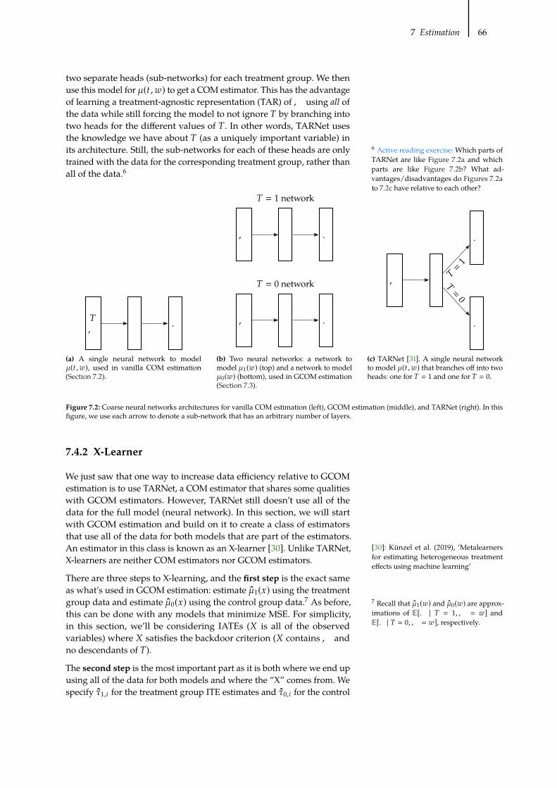
7 Estimation 66
[30]: Künzel et al. (2019), ‘Metalearners
for estimating heterogeneous treatment
effects using machine learning’
7Recall that �1(F) and �0(F) are approx-
imations of E[. | ) = 1,, = F] andE[. | ) = 0,, = F], respectively.
two separate heads (sub-networks) for each treatment group. We then
use this model for �(C , F) to get a COM estimator. This has the advantage
of learning a treatment-agnostic representation (TAR) of, using all ofthe data while still forcing the model to not ignore ) by branching into
two heads for the different values of ). In other words, TARNet uses
the knowledge we have about ) (as a uniquely important variable) in
its architecture. Still, the sub-networks for each of these heads are only
trained with the data for the corresponding treatment group, rather than
all of the data.6
6Active reading exercise: Which parts of
TARNet are like Figure 7.2a and which
parts are like Figure 7.2b? What ad-
vantages/disadvantages do Figures 7.2a
to 7.2c have relative to each other?
),
.
(a) A single neural network to model
�(C , F), used in vanilla COM estimation
(Section 7.2).
, .
, .
) = 1 network
) = 0 network
(b) Two neural networks: a network to
model �1(F) (top) and a network to model
�0(F) (bottom), used in GCOM estimation
(Section 7.3).
.
.
,
)=
1
)=
0
(c) TARNet [31]. A single neural network
to model �(C , F) that branches off into two
heads: one for ) = 1 and one for ) = 0.
Figure 7.2: Coarse neural networks architectures for vanilla COM estimation (left), GCOM estimation (middle), and TARNet (right). In this
figure, we use each arrow to denote a sub-network that has an arbitrary number of layers.
7.4.2 X-Learner
We just saw that one way to increase data efficiency relative to GCOM
estimation is to use TARNet, a COM estimator that shares some qualities
with GCOM estimators. However, TARNet still doesn’t use all of the
data for the full model (neural network). In this section, we will start
with GCOM estimation and build on it to create a class of estimators
that use all of the data for both models that are part of the estimators.
An estimator in this class is known as an X-learner [30]. Unlike TARNet,
X-learners are neither COM estimators nor GCOM estimators.
There are three steps to X-learning, and the first step is the exact same
as what’s used in GCOM estimation: estimate �1(G) using the treatment
group data and estimate �0(G) using the control group data.7As before,
this can be done with any models that minimize MSE. For simplicity,
in this section, we’ll be considering IATEs (- is all of the observed
variables) where - satisfies the backdoor criterion (- contains, and
no descendants of )).
The second step is the most important part as it is both where we end up
using all of the data for both models and where the “X” comes from. We
specify �1,8 for the treatment group ITE estimates and �0,8 for the control

7 Estimation 67
[30]: Künzel et al. (2019), ‘Metalearners
for estimating heterogeneous treatment
effects using machine learning’
[32]: Rosenbaum and Rubin (1983), ‘The
central role of the propensity score in ob-
servational studies for causal effects’
group ITE estimates:
�1,8 = .8(1) − �0(G8) (7.14)
�0,8 = �1(G8) − .8(0) (7.15)
Here, �1,8 is estimated using the treatment group outcomes and the
imputed counterfactual that we get from �0. Similarly, �0,8 is estimated
using the control group outcomes and the imputed counterfactual thatwe
get from �1. If you draw a line between the observed potential outcomes
and a line between the imputed potential outcomes, you can see the
“X” shape. Importantly, this “X” tells us that each treatment group ITE
estimate �1,8 uses both treatment group data (its observed potential
outcome under treatment), and control group data (in �0). Similarly, �0,8
is estimated with data from both treatment groups.
However, each ITE estimate only uses a single data point from its
corresponding treatment group. We can fix this by fitting a model �1(G)to predict �1,8 from the corresponding treatment group G8 ’s. Finally, we
have a model �1(G) that was fit using all of the data (treatment group
data just now and control group data when �0 was fit in step 1). Similarly,
we can fit a model �0(G) to predict �0,8 from the corresponding controlgroup G8 ’s. The output of step 2 is two different estimators for the IATE:
�1(G) and �0(G).
Finally, in step 3, we combine �1(G) and �0(G) together to get our IATE
estimator:
�(G) = 6(G) �0(G) + (1 − 6(G)) �1(G) (7.16)
where 6(G) is some weighting function that produces values between 0
and 1. Künzel et al. [30] report that an estimate of the propensity score
(introduced in next section) works well, but that choosing the constant
function 0 or 1 also makes sense if the treatment groups are very different
sizes. Or that choosing 6(G) to minimize the variance of �(G) could also
be attractive.
Active reading exercise: In this section,
we covered the X-learner for IATE estima-
tion. What would an X-learner for more
general CATE estimation (- is arbitrary
and doesn’t necessarily contain all con-
founders,) look like?
7.5 Propensity Scores
Given that the vector of variables, satisfies the backdoor criterion (or,
equivalently, that (.(1), .(0)) ⊥⊥ ) | ,), we might wonder if it is really
necessary to condition on that whole vector to isolate causal association,
especially when, is high-dimensional. It turns out that it isn’t. If,
satisfies unconfoundedness and positivity, then we can actually get away
with only conditioning on the scalar %() = 1 | ,). We’ll let 4(F) denote%() = 1 | , = F), as we’ll refer to 4(F) as the propensity score since it isthe propensity for (probability of) receiving treatment given that, is
F. The magic of being able to condition on the scalar 4(,) in the place
of the vector, is due to Rosenbaum and Rubin [32]’s propensity score
theorem:
Theorem 7.1 (Propensity Score Theorem) Given positivity, unconfound-edness given, implies unconfoundedness given the propensity score 4(,).

7 Estimation 68
,
) .
Figure 7.3:Simple graphwhere, satisfies
the backdoor criterion
,
) .
Figure 7.5: Simple graph where , con-
founds the effect of ) on .
,
) .
Figure 7.6: Effective graph for pseudo-
population that we get by reweighting
the data generated according to the graph
in Figure 7.5 using inverse probability
weighting.
Equivalently,
(.(1), .(0)) ⊥⊥ ) | , =⇒ (.(1), .(0)) ⊥⊥ ) | 4(,) . (7.17)
We provide a more traditional mathematical proof in Appendix A.2 and
give a graphical proof here. Consider the graph in Figure 7.3. Because
the edge from , to ) is a symbol for the mechanism %() | ,) andbecause the propensity score completely describes that distribution
(%() = 1 | ,) = 4(,)), we can think of the propensity score as a full
mediator of the effect of, on ). This means that we can redraw this
graph with 4(,) situated between , and ). And in this redrawned
graph in Figure 7.4, we can see that 4(,) blocks all backdoor paths that, blocks, so 4(,)must be a sufficient adjustment set if, is. Therefore,
we have a graphical proof of the propensity score theorem using the
backdoor adjustment (Theorem 4.2).
,
4(,)
) .
Figure 7.4: Graph illustrating that 4(,)blocks the backdoor path(s) that, blocks.
Importantly, this theorem means that we can swap in 4(,) in place of,
wherever we are adjusting for, in a given estimator in this chapter. For
example, this seems very useful when, is high-dimensional.
Recall The Positivity-Unconfoundedness Tradeoff from Section 2.3.4. As
we condition on more non-collider-bias-inducing variables, we decrease
confounding. However, this comes at the cost of decreasing overlap
because the, in %() = 1 | ,) becomes higher and higher dimensional.
The propensity score seems to allow us to magically fix that issue since
the 4(,) remains a scalar, even as , grows in dimension. Fantastic,
right?
Well, unfortunately, we usually don’t have access to 4(,). Rather, thebest we can do is model it. We do this by training a model to predict )
from, . For example, logistic regression (logit model) is very commonly
used to do this. And because this model is fit to the high-dimensional, ,
in some sense, we have just shifted the positivity problem to our model
for 4(,).
7.6 Inverse Probability Weighting (IPW)
What if we could resample the data in a way to make it so that association
is causation? This is themotivation behind creating “pseudo-populations”
that are made up of reweighted versions of the observed population. To
get to this, let’s recall why association is not causation in general.
Association is not causation in the graph in Figure 7.5 because, is a
common cause of ) and .. In other words, the mechanism that generates
) depends on , , and the mechanism that generates . depends on
, . Focusing on the mechanism that generates ), we can write this
mathematically as %() | ,) ≠ %()). It turns out that we can reweight
the data to get a pseudo-population where %() | ,) = %()) or %() | ,)equals some constant; the important part is that we make ) independent
of, . The corresponding graph for such a pseudo-population has no
edge from, to ) because ) does not depend on, ; we depict this in
Figure 7.6.
It turns out that the propensity score is key to this reweighting. All we
have to do is reweight each data point with treatment ) and confounders
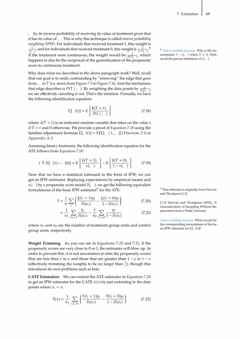
7 Estimation 69
8Active reading exercise: Why is the de-
nominator 1 − 4(,) when ) = 0. Hint:
recall the precise definition of 4(,).
9This estimator is originally fromHorvitz
and Thompson [33]
[33]: Horvitz and Thompson (1952), ‘A
Generalization of Sampling Without Re-
placement from a Finite Universe’
.
, by its inverse probability of receiving its value of treatment given that
it has its value of, . This is why this technique is called inverse probabilityweighting (IPW). For individuals that received treatment 1, this weight is
1
4(,) , and for individuals that received treatment 0, this weight is1
1−4(,) .8
If the treatment were continuous, the weight would be1
%() |,) , which
happens to also be the reciprocal of the generalization of the propensity
score to continuous treatment.
Why does what we described in the above paragraph work? Well, recall
that our goal is to undo confounding by “removing” the edge that goes
from, to) (i.e. move from Figure 7.5 to Figure 7.6). And the mechanism
that edge describes is %() | ,). By weighting the data points by1
%() |,) ,we are effectively canceling it out. That’s the intuition. Formally, we have
the following identification equation:
E[.(C)] = E
[1() = C).%(C | ,)
](7.18)
where 1() = C) is an indicator random variable that takes on the value 1
if ) = C and 0 otherwise. We provide a proof of Equation 7.18 using the
familiar adjustment formula E[.(C)] = E[E[. | C ,,]] (Theorem 2.1) in
Appendix A.3.
Assuming binary treatment, the following identification equation for the
ATE follows from Equation 7.18:
� , E[.(1) − .(0)] = E
[1() = 1).4(,)
]− E
[1() = 0).1 − 4(,)
](7.19)
Now that we have a statistical estimand in the form of IPW, we can
get an IPW estimator. Replacing expectations by empirical means and
4(,) by a propensity score model 4(,), we get the following equivalent
formulations of the basic IPW estimator9for the ATE:
� =1
=
∑8
(1(C8 = 1)H84(F8)
−1(C8 = 0)H81 − 4(F8)
)(7.20)
=1
=1
∑8:C8=1
H8
4(F8)− 1
=0
∑8:C8=0
H8
1 − 4(F8)(7.21)
where =1 and =0 are the number of treatment group units and control
group units, respectively.
Active reading exercise: What would be
the corresponding formulations of the ba-
sic IPW estimator for E[.(C)]?
Weight Trimming As you can see in Equations 7.20 and 7.21, if the
propensity scores are very close to 0 or 1, the estimates will blow up. In
order to prevent this, it is not uncommon to trim the propensity scores
that are less than & to & and those that are greater than 1 − & to 1 − &(effectively trimming the weights to be no larger than
1
& ), though this
introduces its own problems such as bias.
CATE Estimation We can extend the ATE estimator in Equation 7.20
to get an IPW estimator for the CATE �(G) by just restricting to the data
points where G8 = G:
�(G) = 1
=G
∑8:G8=G
(1(C8 = 1)H84(F8)
−1(C8 = 0)H81 − 4(F8)
)(7.22)

7 Estimation 70
[34]: Abrevaya et al. (2015), ‘Estimating
Conditional Average Treatment Effects’
10An estimator is consistent if it converges
in probability to its estimand as the num-
ber of samples = grows.
[35]: Kang and Schafer (2007), ‘Demysti-
fying Double Robustness: A Comparison
of Alternative Strategies for Estimating a
Population Mean from Incomplete Data’
[36]: Zivich and Breskin (2020), Machinelearning for causal inference: on the use ofcross-fit estimators
[37]: Dorie et al. (2019), ‘Automated versus
Do-It-Yourself Methods for Causal Infer-
ence: Lessons Learned from a Data Analy-
sis Competition’
[38]: Seaman and Vansteelandt (2018), ‘In-
troduction to Double Robust Methods for
Incomplete Data’
[39]: Tsiatis (2007), Semiparametric theoryand missing data[40]: Robins et al. (1994), ‘Estimation of
Regression Coefficients When Some Re-
gressors are not Always Observed’
[41]: Bang and Robins (2005), ‘Doubly
Robust Estimation in Missing Data and
Causal Inference Models’
[42]: Van Der Laan and Rubin (2006), ‘Tar-
geted maximum likelihood learning’
[43]: Schuler and Rose (2017), ‘Targeted
Maximum Likelihood Estimation for
Causal Inference inObservational Studies’
[44]: Van der Laan andRose (2011),Targetedlearning: causal inference for observational andexperimental data
where =G is the number of data pointswith G8 = G. However, the estimator
in Equation 7.22 may quickly run into the problem of using very small
amounts of data, leading to high variance. More general CATE estimation
with IPW estimators is more complex and outside the scope of this book.
See, for example, Abrevaya et al. [34] and references therein.
7.7 Doubly Robust Methods
We’ve seen that we can estimate causal effects by modeling �(C , F) ,E[. | C , F] (Sections 7.2 to 7.4) or by modeling 4(F) , %() = 1 | F)(Section 7.6). What if we modeled both �(C , F) and 4(F)? Well, we can
and estimators that do this are sometimes doubly robust. A doubly robust
estimator has the property that it is a consistent10estimator of � if either
� is a consistent estimator of � or 4 is a consistent estimate of 4. In other
words, only one of � and 4 needs to be well-specified. Additionally, the
rate at which a doubly robust estimator converges to � is the product ofthe rate at which � converges to � and the rate at which 4 converges to 4.
This makes double robustness is very useful when we are using flexible
machine learning models in high-dimensions because, in this setting,
each of our individual models (� and 4) converge more slowly that the
ideal rate of =−1/2.
However, there is some controversy over how well doubly robust meth-
ods work in practice if not at least one of � or 4 is well-specified [35].
Though, this might be contested as we get better at using doubly ro-
bust estimators with flexible machine learning models (see, e.g., [36]).
Meanwhile, the estimators that currently seem to do the best all flexibly
model � (unlike pure IPW estimators) [37]. This is why we began this
chapter with estimators that model � and dedicated several sections to
such estimators.
Doubly robust methods are largely outside the scope of this book, so
we refer the reader to an introduction by Seaman and Vansteelandt [38],
along with other seminal works on the topic: [39–41]. Additionally, there
is a large body of doubly robust work on methods that have performed
reasonably well in competitions [37]; this category is known as targetedmaximum likelihood estimation (TMLE). [42–44].
7.8 Other Methods
As this chapter is only an introduction to estimation in causal inference,
there are some methods that we’ve entirely left out. We’ll briefly describe
some of the most popular ones in this section.
Matching In matching methods, we try to match units in the treatment
group with units in the control group and throw away the non-matches
to create comparable groups. We can match in raw covariate space,
coarsened covariate space, or propensity score space. There are different
distance functions for deciding how close two units are. Furthermore,
there are different criteria for deciding whether a given distance is close
enough to count as a match (one criterion requires an exact match), how
many matches each treatment group unit can have, how many matches

7 Estimation 71
[45]: Stuart (2010), ‘Matching Methods for
Causal Inference: A Review and a Look
Forward’
11Active reading exercise: How is this
model different from �?
[46]: Chernozhukov et al. (2018), ‘Dou-
ble/debiased machine learning for treat-
ment and structural parameters’
[47]: Felton (2018), Chernozhukov et al. onDouble / Debiased Machine Learning[48]: Syrgkanis (2019), Orthogonal/DoubleMachine Learning[49]: Foster and Syrgkanis (2019), Orthogo-nal Statistical Learning
[50]: Athey and Imbens (2016), ‘Recursive
partitioning for heterogeneous causal ef-
fects’
[51]: Wager and Athey (2018), ‘Estima-
tion and Inference of Heterogeneous Treat-
ment Effects using Random Forests’
[52]: Athey et al. (2019), ‘Generalized ran-
dom forests’
each control group unit can have, etc. See, for example, Stuart [45] for a
review.
Double Machine Learning In double machine learning, we fit three
models in two stages: two in the first stage and a final model in the second
stage. First stage:
1. Fit a model to predict . from, to get the predicted ..11
2. Fit a model to predict ) from, to get the to get the predicted ).
Then, in the second stage, we “partial out”, by looking at . − . and
) − ). In a sense, we have deconfounded the effect of treatment on the
outcome with this partialling out. Then, we fit a model to predict . − .from ) − ). This gives us our causal effect estimates. For more on this
topic, see, for example [46–49].
Causal Trees and Forests Another popular estimation method is to
recursively partition the data into subsets that have the same treatment
effects [50]. This forms a causal tree where the leaves are subsets of the
population with similar causal effects. Since random forests generally
perform better than decision trees, it would be great if this kind of
strategy can be extended to random forests. And it can. This extensions
is known as causal forests [51], which are part of more general class
known as generalized random forests [52]. Importantly, these methods were
developed with the goal in mind of yielding valid confidence intervals
for the estimates.
7.9 Concluding Remarks
7.9.1 Confidence Intervals
So far, in this chapter, we have only discussed point estimates for causal
effects. We haven’t discussed how we can gauge our uncertainty due
to data sampling. We haven’t discussed how to calculate confidence
intervals on these estimates. This is a machine learning perspective, after
all; who cares about confidence intervals... Jokes aside, because we are
allowing for arbitrary machine learning models in all of the estimators
we discuss, it is actually quite difficult to get valid confidence intervals.
Bootstrapping One way to get confidence intervals is to use bootstrap-
ping. With bootstrapping, we repeat the causal effect estimation process
many times, each time with a different sample (with replacement) from
our data. This allows us to build an empirical distribution for the estimate.
We can then compute whatever confidence interval we like from that em-
pirical distribution. Unfortunately, bootstrapped confidence intervals are
not always valid. For example, if we take a bootstrapped 95% confidence
interval, it might not contain the true value (estimand) 95% of the time.
Specialized Models Another way to get confidence intervals is to
analyze very specific models, rather than allowing for arbitrary models
Linear models are the simplest example of this; it is easy to get confidence
intervals in linearmodels. Similarly, if we use a linearmodel as the second
stage model in double machine learning, we can get confidence intervals.
Noticeably, causal trees and causal forests were developed with the goal
in mind of getting confidence intervals.

7 Estimation 72
7.9.2 Comparison to Randomized Experiments
You might read somewhere that some of these adjustment techniques
ensure that we’ve addressed confounding and isolated a causal effect.
Of course, this is not true when there is unobserved confounding. These
methods only address observed confounding. If there are any unobserved
confounders, these methods don’t fix that like randomization does
(Chapter 5). These adjustment methods aren’t magic. And it’s hard to
know when it is reasonable to assume we’ve observed all confounders.
That’s why it is important to run a sensitivity analysis where we gauge
how robust our causal effect estimates are to unobserved confounding.
This is the topic of the next chapter.
Active reading exercise: What kind of estimator did we use back in the
estimation examples in Sections 2.5 and 4.6.2?

[53]: Manski (2003), Partial Identification ofProbability Distributions: Springer Series inStatistics
[54]: Manski (1989), ‘Anatomy of the Selec-
tion Problem’
[55]: Manski (1990), ‘Nonparametric
Bounds on Treatment Effects’
[56]: Manski (1993), ‘Identification Prob-
lems in the Social Sciences’
[57]: Manski (1994), ‘The selection prob-
lem’
[58]: Manski (1997), ‘Monotone Treatment
Response’
[59]: Manski and Pepper (2000), ‘Mono-
tone Instrumental Variables: With an Ap-
plication to the Returns to Schooling’
[53]: Manski (2003), Partial Identification ofProbability Distributions: Springer Series inStatistics[60]: Manski (2013), Public Policy in an Un-certain World
Unobserved Confounding:Bounds and Sensitivity Analysis 8
8.1 Bounds . . . . . . . . . . . . . 73No-Assumptions Bound . . 74Monotone Treatment Re-sponse . . . . . . . . . . . . . 76
Monotone Treatment Selec-tion . . . . . . . . . . . . . . . 78
Optimal Treatment Selection798.2 Sensitivity Analysis . . . . . 82
Sensitivity Basics in LinearSetting . . . . . . . . . . . . 82
More General Settings . . . 85
All of themethods inChapter 7 assume thatwedon’t have anyunobserved
confounding. However, unconfoundedness is an untestable assumption.
In observational studies, there could also be some unobserved con-
founder(s). Therefore, we’d like to know how robust our estimates are
to unobserved confounding. The first way we can do is by getting an
upper and lower bound on the causal effect using credible assumptions
(Section 8.1). Another way we can do this is by simulating how strong the
confounder’s effect on the treatment and the confounder’s effect on the
outcome need to be to make the true causal effect substantially different
from our estimate (Section 8.2).
,
) .
(a) No unobserved confounding
, *
) .
(b) Unobserved confounding (*)
Figure 8.1: On the left, we have the setting we have considered up till now, where we have
unconfoundedness / the backdoor criterion. On the right, we have a simple graph where
the unobserved confounder* make the causal effect of ) on . not identifiable.
8.1 Bounds
There is a tradeoff between how realistic or credible our assumptions
are and how precise of an identification result we can get. Manski [53]
calls this “The Law of Decreasing Credibility: the credibility of inference
decreases with the strength of the assumptions maintained.”
Depending on what assumptions we are willing to make, we can derive
various nonparametric bounds on causal effects. We have seen that if
we are willing to assume unconfoundedness (or some causal graph in
which the causal effect is identifiable) and positivity, we can identify a
single point for the causal effect. However, this might be unrealistic. For
example, there could always be unobserved confounding in observational
studies.
This is what motivates Charles Manski’s work on bounding causal effects
[53–60]. This gives us an interval that the causal effect must be in, rather
than telling us exactly what point in that interval the causal effect must
be. In this section, we will give an introduction to these nonparametric
bounds and how to derive them.
The assumptions that we consider are weaker than unconfoundedness,
so they give us intervals that the causal effect must fall in (under these

8 Unobserved Confounding: Bounds and Sensitivity Analysis 74
[55]: Manski (1990), ‘Nonparametric
Bounds on Treatment Effects’
Active reading exercise: Ensure you follow
how we get to these bounds.
assumptions). If we assumed the stronger assumption of unconfounded-
ness, these intervals would collapse to a single point. This illustrates the
law of decreasing credibility.
8.1.1 No-Assumptions Bound
Say all we know about the potential outcomes .(0) and .(1) is that theyare between 0 and 1. Then, the maximum value of an ITE .8(1) − .8(0) is1 (1 - 0), and the minimum is -1 (0 - 1):
−1 ≤ .8(1) − .8(0) ≤ 1 if ∀C , 0 ≤ .(C) ≤ 1 (8.1)
So we know that all ITEs must be in an interval of length 2. Because
all the ITEs must fall inside this interval of length 2, the ATE must also
fall inside this interval of length 2. Interestingly, for ATEs, it turns out
that we can cut the length of this interval in half without making any
assumptions (beyond the min/max value of outcome); the interval that
the ATE must fall in is only of length 1.
We’ll show this result from Manski [55] in the more general scenario
where the outcome is bounded between 0 and 1:
Assumption 8.1 (Bounded Potential Outcomes)
∀C , 0 ≤ .(C) ≤ 1 (8.2)
By the same reasoning as above, this implies the following bounds on
the ITEs and ATE:
0 − 1 ≤ .8(1) − .8(0) ≤ 1 − 0 (8.3)
0 − 1 ≤ E[.(1) − .(0)] ≤ 1 − 0 (8.4)
These are intervals of length (1−0)−(0−1) = 2(1−0). And the bounds for
the ITEs cannot be made tighter without further assumptions. However,
seemingly magically, we can halve the length of the interval for the ATE.
To see this, we rewrite the ATE as follows:
E[.(1) − .(0)] = E[.(1)] − E[.(0)] (8.5)
= %() = 1)E[.(1) | ) = 1] + %() = 0)E[.(1) | ) = 0]− %() = 1)E[.(0) | ) = 1] − %() = 0)E[.(0) | ) = 0]
(8.6)
We immediately recognize the first and last terms as friendly conditional
expectations that we can estimate from observational data:
= %() = 1)E[. | ) = 1] + %() = 0)E[.(1) | ) = 0]− %() = 1)E[.(0) | ) = 1] − %() = 0)E[. | ) = 0]
(8.7)
Active reading exercise: What assumption
are we using here?
Because this is such an important decomposition, we’ll give it a name
and box before moving on with the bound derivation. We will call this
the observational-counterfactual decomposition (of the ATE). Also, to have

8 Unobserved Confounding: Bounds and Sensitivity Analysis 75
a bit more concise notation, we’ll use � , %() = 1) moving forward.
Proposition 8.1 (Observational-Counterfactual Decomposition)
E[.(1) − .(0)] = �E[. | ) = 1] + (1 − �)E[.(1) | ) = 0]− �E[.(0) | ) = 1] − (1 − �)E[. | ) = 0] (8.8)
Unfortunately, E[.(1) | ) = 0] and E[.(0) | ) = 1] are counterfactual.
However, we know that they’re bounded between 0 and 1. Therefore, we
get an upper bound on the complete expression by letting the quantity
that’s being added (E[.(1) | ) = 0]) equal 1 and letting the quantity
that’s being subtracted (E[.(0) | ) = 1]) equal 0. Similarly, we can get a
lower bound by letting the term that’s being added equal 0 and the term
that’s being subtracted equal 1.
Proposition 8.2 (No-Assumptions Bound) Let � denote %() = 1), where) is a binary random variable. Given that the outcome . is bounded between0 and 1 (Assumption 8.1), we have the following upper and lower bounds onthe ATE:
E[.(1)−.(0)] ≤ �E[. | ) = 1]+ (1−�) 1−� 0−(1−�)E[. | ) = 0](8.9)
E[.(1)−.(0)] ≥ �E[. | ) = 1]+ (1−�) 0−� 1−(1−�)E[. | ) = 0](8.10)
Importantly, the length of this interval is 1 − 0, half the length of the
naive interval that we saw in Equation 8.4. We can see this by subtracting
the lower bound from the upper bound:
�E[. | ) = 1] + (1 − �) 1 − � 0 − (1 − �)E[. | ) = 0]−(�E[. | ) = 1] + (1 − �) 0 − � 1 − (1 − �)E[. | ) = 0])
= (1 − �) 1 + � 1 − � 0 − (1 − �) 0 (8.11)
= 1 − 0 (8.12)
This is sometimes referred to as the “no-assumptions bound” because
we made no assumptions other than that the outcomes are bounded. If
the outcomes are not bounded, then the ATE and ITEs can be anywhere
between −∞ and∞.
Running Example
Consider that we know that the outcomes are bounded between 0
and 1 (e.g., because we’re in a binary outcomes setting). This means
that the ITEs and must be bounded between -1 (0 - 1) and 1 (1 - 0),
which means that the ATE must also be bounded between -1 and
1. For this example, also consider that � = 0.3, E[. | ) = 1] = .9,
and E[. | ) = 0] = .2.1 1Active reading exercise: How would we
estimate these conditional expectations?
Then, by plugging these in to Equations 8.9
and 8.10, we get the following bounds on the ATE:
E[.(1) − .(0)] ≤ (.3)(.9) + (1 − .3)(1) − (.3)(0) − (1 − .3)(.2) (8.13)
E[.(1) − .(0)] ≥ (.3)(.9) + (1 − .3)(0) − (.3)(1) − (1 − .3)(.2) (8.14)

8 Unobserved Confounding: Bounds and Sensitivity Analysis 76
2To see why the no-assumptions bound
always contains zero, consider what we
would need for it to not contain zero: we
would either need the upper bound to
be less than zero or the lower bound to
be greater than zero. However, this can-
not be the case. To see why, note that the
minimum upper bound is achieved when
E[. | ) = 1] = 0 and E[. | ) = 0] = 1,
which gives us an (inclusive) upper bound
of zero. Same with the lower bound.
Active reading exercise: Show that the
maximum lower bound is 0.
[58]: Manski (1997), ‘Monotone Treatment
Response’
−0.17 ≤ E[.(1) − .(0)] ≤ 0.83 (8.15)
Notice that this interval is of length 1 (1 − 0 = 1), half the length of
the naive interval −1 ≤ E[.(1) − .(0)] ≤ 1 (Equation 8.4). We will
use this running example throughout Section 8.1.
Active reading exercises:
1. What kind of bounds can we get for CATEs E[.(1) − .(0) | -],assuming we have positivity? What goes wrong if we don’t have
positivity?
2. Say the potential outcomes are bounded in different ways: 01 ≤.(1) ≤ 11 and 00 ≤ .(0) ≤ 10. Derive the corresponding no-
assumptions bounds in this more general setting.
The bounds in Proposition 8.2 are as tight as we can get without further
assumptions. Unfortunately, the corresponding interval always contains
0,2which means that we cannot use this bound to distinguish “no causal
effect” from “causal effect.” Can we get tighter bounds?
In order to bound the ATE, we must have some information about the
counterfactual part of this decomposition. We can easily estimate the
observational part from data. In the no-assumptions bound (Proposi-
tion 8.2), all we assumed is that the outcomes are bounded by 0 and 1.
If we make more assumptions, we can get smaller intervals. In the next
few sections, we will cover some assumptions that are sometimes fairly
reasonable, depending on the setting, and what tighter bounds these
assumptions get us. The general strategy we will use for all of them is to
start with the observational-counterfactual decomposition of the ATE
(Proposition 8.1),
E[.(1) − .(0)] = �E[. | ) = 1] + (1 − �)E[.(1) | ) = 0]− �E[.(0) | ) = 1] − (1 − �)E[. | ) = 0] ,
(8.8 revisited)
and get smaller intervals by bounding the counterfactual parts using the
different assumptions we make.
The intervals we will see in the next couple of subsections will all contain
zero. We won’t see an interval that is purely positive or purely negative
until Section 8.1.4, so feel free to skip to that section if you only want to
see those intervals.
8.1.2 Monotone Treatment Response
For our first assumption beyond assuming bounded outcomes, consider
that we find ourselves in a setting where it is feasible that the treatment
can only help; it can’t hurt. This is the setting that Manski [58] considers
in context. In this setting, we can justify the monotone treatment response(MTR) assumption:
Assumption 8.2 (Nonnegative Monotone Treatment Response)
∀8 .8(1) ≥ .8(0) (8.16)

8 Unobserved Confounding: Bounds and Sensitivity Analysis 77
3Recall that by only assuming that out-
comes are bounded between 0 and 1,
we get the no-assumptions lower bound
(Proposition 8.2):
E[.(1) − .(0)]≥ �E[. | ) = 1] + (1 − �) 0− � 1 − (1 − �)E[. | ) = 0]
(8.10 revisited)
4Recall the no-assumptions upper bound
(Proposition 8.2):
E[.(1) − .(0)]≤ �E[. | ) = 1] + (1 − �) 1− � 0 − (1 − �)E[. | ) = 0]
(8.9 revisited)
5Recall the no-assumptions lower bound
(Proposition 8.2):
E[.(1) − .(0)]≥ �E[. | ) = 1] + (1 − �) 0− � 1 − (1 − �)E[. | ) = 0]
(8.10 revisited)
This means that every ITE is nonnegative, so we can bring our lower
bound on the ITEs up from 0 − 1 (Equation 8.3) to 0. So, intuitively, this
should mean that our lower bound on the ATE should move up to 0. And
we will now see that this is the case.
Now, rather than lower bounding E[.(1) | ) = 0]with 0 and −E[.(0) |) = 1] with −1, we can do better. Because the treatment only helps,
E[.(1) | ) = 0] ≥ E[.(0) | ) = 0] = E[. | ) = 0], so we can lower
bound E[.(1) | ) = 0] with E[. | ) = 0]. Similarly, −E[.(0) | ) = 1] ≥−E[.(1) | ) = 1] = E[. | ) = 1] (sincemultiplying by a negative flips the
inequality), so we can lower bound −E[.(0) | ) = 1]with −E[. | ) = 1].Therefore, we can improve on the no-assumptions lower bound
3to get 0,
as our intuition suggested:
E[.(1) − .(0)] = �E[. | ) = 1] + (1 − �)E[.(1) | ) = 0]− �E[.(0) | ) = 1] − (1 − �)E[. | ) = 0]
(8.8 revisited)
≥ �E[. | ) = 1] + (1 − �)E[. | ) = 0]− �E[. | ) = 1] − (1 − �)E[. | ) = 0] (8.17)
= 0 (8.18)
Proposition 8.3 (Nonnegative MTR Lower Bound) Under the nonnega-tive MTR assumption, the ATE is bounded from below by 0. Mathematically,
E[.(1) − .(0)] ≥ 0 (8.19)
Running Example The no-assumptions upper bound4still applies here,
so in our running example from Section 8.1.1 where� = .3,E[. | ) = 1] =.9, and E[. | ) = 0] = .2, our ATE interval improves from [−0.17, 0.83](Equation 8.15) to [0, 0.83].
Alternatively, say the treatment can only hurt people; it can’t help them
(e.g. a gunshot wound only hurts chances of staying alive). In those cases,
we would have the nonpositive monotone treatment response assumption
and the nonpositive MTR upper bound:
Assumption 8.3 (Nonpositive Monotone Treatment Response)
∀8 .8(1) ≤ .8(0) (8.20)
Active reading exercise: Prove Proposi-
tion 8.4.
Proposition 8.4 (Nonpositive MTRUpper Bound) Under the nonpositiveMTR assumption, the ATE is bounded from above by 0. Mathematically,
E[.(1) − .(0)] ≤ 0 (8.21)
Running Example And in this setting, the no-assumptions lower
bound5still applies. That means that the ATE interval in our exam-
ple improves from [−0.17, 0.83] (Equation 8.15) to [−0.17, 0].
Active reading exercise: What is the ATE interval if we assume both non-
negative MTR and nonpositive MTR? Does this make sense, intuitively?
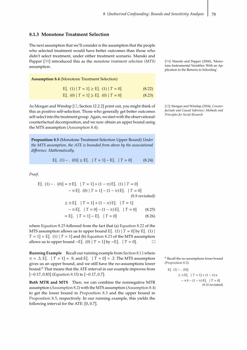
8 Unobserved Confounding: Bounds and Sensitivity Analysis 78
[59]: Manski and Pepper (2000), ‘Mono-
tone Instrumental Variables: With an Ap-
plication to the Returns to Schooling’
[12]: Morgan and Winship (2014), Counter-factuals and Causal Inference: Methods andPrinciples for Social Research
8.1.3 Monotone Treatment Selection
The next assumption that we’ll consider is the assumption that the people
who selected treatment would have better outcomes than those who
didn’t select treatment, under either treatment scenario. Manski and
Pepper [59] introduced this as the monotone treatment selection (MTS)assumption.
Assumption 8.4 (Monotone Treatment Selection)
E[.(1) | ) = 1] ≥ E[.(1) | ) = 0] (8.22)
E[.(0) | ) = 1] ≥ E[.(0) | ) = 0] (8.23)
As Morgan andWinship [12, Section 12.2.2] point out, you might think of
this as positive self-selection. Those who generally get better outcomes
self-select into the treatment group.Again,we startwith the observational-
counterfactual decomposition, and we now obtain an upper bound using
the MTS assumption (Assumption 8.4):
Proposition 8.5 (Monotone Treatment Selection Upper Bound) Underthe MTS assumption, the ATE is bounded from above by the associationaldifference. Mathematically,
E[.(1) − .(0)] ≤ E[. | ) = 1] − E[. | ) = 0] (8.24)
Proof.
E[.(1) − .(0)] = �E[. | ) = 1] + (1 − �)E[.(1) | ) = 0]− �E[.(0) | ) = 1] − (1 − �)E[. | ) = 0]
(8.8 revisited)
≤ �E[. | ) = 1] + (1 − �)E[. | ) = 1]− �E[. | ) = 0] − (1 − �)E[. | ) = 0] (8.25)
= E[. | ) = 1] − E[. | ) = 0] (8.26)
where Equation 8.25 followed from the fact that (a) Equation 8.22 of the
MTS assumption allows us to upper bound E[.(1) | ) = 0] by E[.(1) |) = 1] = E[.(1) | ) = 1] and (b) Equation 8.23 of the MTS assumption
allows us to upper bound −E[.(0) | ) = 1] by −E[. | ) = 0].
Running Example Recall our running example fromSection 8.1.1 where
� = .3, E[. | ) = 1] = .9, and E[. | ) = 0] = .2. The MTS assumption
gives us an upper bound, and we still have the no-assumptions lower
bound.6
6Recall the no-assumptions lower bound
(Proposition 8.2):
E[.(1) − .(0)]≥ �E[. | ) = 1] + (1 − �) 0− � 1 − (1 − �)E[. | ) = 0]
(8.10 revisited)
That means that the ATE interval in our example improves from
[−0.17, 0.83] (Equation 8.15) to [−0.17, 0.7].
Both MTR and MTS Then, we can combine the nonnegative MTR
assumption (Assumption 8.2) with theMTS assumption (Assumption 8.4)
to get the lower bound in Proposition 8.3 and the upper bound in
Proposition 8.5, respectively. In our running example, this yields the
following interval for the ATE: [0, 0.7].

8 Unobserved Confounding: Bounds and Sensitivity Analysis 79
[55]: Manski (1990), ‘Nonparametric
Bounds on Treatment Effects’
7Recall the no-assumptions upper bound
(Proposition 8.2):
E[.(1) − .(0)]≤ �E[. | ) = 1] + (1 − �) 1− � 0 − (1 − �)E[. | ) = 0]
(8.9 revisited)
8Recall the no-assumptions lower bound
(Proposition 8.2):
E[.(1) − .(0)]≥ �E[. | ) = 1] + (1 − �) 0− � 1 − (1 − �)E[. | ) = 0]
(8.10 revisited)
Intervals Contain Zero Although bounds from the MTR and MTS
assumptions can be useful for ruling out very large or very small causal
effects, the corresponding intervals still contain zero. This means that
these assumptions are not enough to identify whether there is an effect
or not.
8.1.4 Optimal Treatment Selection
We now consider what we will call the optimal treatment selection (OTS) as-sumption from Manski [55]. This assumption means that the individuals
always receive the treatment that is best for them (e.g. if an expert doctor
is decidingwhich treatment to give people).Wewrite this mathematically
as follows:
Assumption 8.5 (Optimal Treatment Selection)
)8 = 1 =⇒ .8(1) ≥ .8(0) , )8 = 0 =⇒ .8(0) > .8(1) (8.27)
From the OTS assumption, we know that
E[.(1) | ) = 0] ≤ E[.(0) | ) = 0] = E[. | ) = 0] . (8.28)
Therefore, we can give an upper bound, by upper bounding
E[.(1) | ) = 0] with E[. | ) = 0] and upper bounding −E[.(0) | ) = 1]with −0 (same as in the no-assumptions upper bound
7):
E[.(1) − .(0)] = �E[. | ) = 1] + (1 − �)E[.(1) | ) = 0]− �E[.(0) | ) = 1] − (1 − �)E[. | ) = 0]
(8.8 revisited)
≤ �E[. | ) = 1] + (1 − �)E[. | ) = 0]− � 0 − (1 − �)E[. | ) = 0] (8.29)
= �E[. | ) = 1] − � 0 (8.30)
The OTS assumption also tells us that
E[.(0) | ) = 1] ≤ E[.(1) | ) = 1] = E[. | ) = 1] , (8.31)
which is equivalent to saying −E[.(0) | ) = 1] ≥ −E[. | ) = 1]. So we
can lower bound −E[.(0) | ) = 1]with −E[. | ) = 1], and we can lower
bound E[.(1) | ) = 0]with 0 (just as we did in the no-assumptions lower
bound8) to get the following lower bound:
E[.(1) − .(0)] = �E[. | ) = 1] + (1 − �)E[.(1) | ) = 0]− �E[.(0) | ) = 1] − (1 − �)E[. | ) = 0]
(8.8 revisited)
≥ �E[. | ) = 1] + (1 − �) 0− �E[. | ) = 1] − (1 − �)E[. | ) = 0] (8.32)
= (1 − �) 0 − (1 − �)E[. | ) = 0] (8.33)

8 Unobserved Confounding: Bounds and Sensitivity Analysis 80
9Active reading exercise: Show that this
interval always contains zero.
[55]: Manski (1990), ‘Nonparametric
Bounds on Treatment Effects’
10Recall the OTS assumption (Assump-
tion 8.5):
)8 = 1 =⇒ .8(1) ≥ .8(0) (8.41)
)8 = 0 =⇒ .8(0) > .8(1) (8.42)
Because there are only two values that
) can take on, this is equivalent to the
following (contrapositives):
)8 = 0 ⇐= .8(1) < .8(0) (8.43)
)8 = 1 ⇐= .8(0) ≤ .8(1) (8.44)
[55]: Manski (1990), ‘Nonparametric
Bounds on Treatment Effects’
Proposition 8.6 (Optimal Treatment Selection Bound 1) Let � denote%() = 1), where ) is a binary random variable. Given that the outcome . isbounded from below by 0 (Assumption 8.1) and that the optimal treatment isalways selection (Assumption 8.5), we have the following upper and lowerbounds on the ATE:
E[.(1) − .(0)] < �E[. | ) = 1] − � 0 (8.34)
E[.(1) − .(0)] ≥ (1 − �) 0 − (1 − �)E[. | ) = 0] (8.35)
Interval Length = �E[. | ) = 1] + (1 − �)E[. | ) = 0] − 0 (8.36)
Unfortunately, this interval also always contains zero!9This means that
Proposition 8.6 doesn’t tell us whether the causal effect is non-zero or
not.
Running Example Recall our running example fromSection 8.1.1 where
0 = 0, 1 = 1, � = .3, E[. | ) = 1] = .9, and E[. | ) = 0] = .2. Plugging
these in to Proposition 8.6 gives us the following:
E[.(1) − .(0)] ≤ (.3) (.9) − (.3) (0) (8.37)
E[.(1) − .(0)] ≥ (1 − .3) (0) − (1 − .3) (.2) (8.38)
−0.14 ≤ E[.(1) − .(0)] ≤ 0.27 (8.39)
Interval Length = 0.41 (8.40)
We’ll now give an interval that can be purely positive or purely negative,
potentially identifying the ATE as non-zero.
A Bound That Can Identify the Sign of the ATE
It turns out that, although we take the OTS assumption from Manski
[55], the bound we gave in Proposition 8.6 is not actually the bound that
Manski [55] derives with that assumption. For example, where we used
E[.(1) | ) = 0] ≤ E[. | ) = 0], Manski uses E[.(1) | ) = 0] ≤ E[. |) = 1]. We’ll quickly prove this inequality that Manski uses from the
OTS assumption:10We start by applying Equation 8.42:
E[.(1) | ) = 0] = E[.(1) | .(0) > .(1)] (8.45)
Because the random variable we are taking the expectation of is .(1), ifwe flip .(0) > .(1) to .(0) ≤ .(1), then we get an upper bound:
≤ E[.(1) | .(0) ≤ .(1)] (8.46)
Finally, applying Equation 8.44, we have the result:
= E[.(1) | ) = 1] (8.47)
= E[. | ) = 1] (8.48)
Now that we have that E[.(1) | ) = 0] ≤ E[. | ) = 1], we can
prove Manski [55]’s upper bound, where we use this key inequality in

8 Unobserved Confounding: Bounds and Sensitivity Analysis 81
[55]: Manski (1990), ‘Nonparametric
Bounds on Treatment Effects’
12Active reading exercise: Using Equa-
tions 8.40 and 8.59, derive the conditions
under which OTS bound 1 yields a smaller
interval and the conditions under which
OTS bound 2 yields a smaller interval.
Equation 8.49:
E[.(1) − .(0)] = �E[. | ) = 1] + (1 − �)E[.(1) | ) = 0]− �E[.(0) | ) = 1] − (1 − �)E[. | ) = 0]
(8.8 revisited)
≤ �E[. | ) = 1] + (1 − �)E[.(1) | ) = 1]− � 0 − (1 − �)E[. | ) = 0] (8.49)
= �E[. | ) = 1] + (1 − �)E[. | ) = 1]− � 0 − (1 − �)E[. | ) = 0] (8.50)
= E[. | ) = 1] − � 0 − (1 − �)E[. | ) = 0] (8.51)
Similarly, we can perform an analogous derivation11
11Active reading exercise: Derive Equa-
tion 8.52 yourself.
to get the lower
bound:
E[.(1) − .(0)] ≥ �E[. | ) = 1] + (1 − �) 0 − E[. | ) = 0] (8.52)
Proposition 8.7 (Optimal Treatment Selection Bound 2) Let � denote%() = 1), where ) is a binary random variable. Given that the outcome . isbounded from below by 0 (Assumption 8.1) and that the optimal treatment isalways selection (Assumption 8.5), we have the following upper and lowerbounds on the ATE:
E[.(1) − .(0)] ≤ E[. | ) = 1] − � 0 − (1 − �)E[. | ) = 0] (8.53)
E[.(1) − .(0)] ≥ �E[. | ) = 1] + (1 − �) 0 − E[. | ) = 0] (8.54)
Interval Length = (1 − �)E[. | ) = 1] + �E[. | ) = 0] − 0 (8.55)
This interval can also include zero, but it doesn’t have to. For example, in
our running example, it doesn’t.
Running Example Recall our running example fromSection 8.1.1 where
0 = 0, 1 = 1, � = .3, E[. | ) = 1] = .9, and E[. | ) = 0] = .2. Plugging
these in to Proposition 8.7 gives us the following for the OTS bound 2:
E[.(1) − .(0)] ≤ (.9) − (.3) (0) − (1 − .3) (.2) (8.56)
E[.(1) − .(0)] ≥ (.3) (.9) + (1 − .3) (0) − (.2) (8.57)
0.07 ≤ E[.(1) − .(0)] ≤ 0.76 (8.58)
Interval Length = 0.69 (8.59)
Application of OTS bound 1 (Proposi-
tion 8.6) to our running example:
−0.14 ≤ E[.(1) − .(0)] ≤ 0.27
(8.39 revisited)
Interval Length = 0.41 (8.40 revisited)
So while the OTS bound 2 fromManski [55] identifies the sign of the ATE
in our running example, unlike the OTS bound 1, the OTS bound 2 gives
us a 68% larger interval. You can see this by comparing Equation 8.40 (in
the above margin) with Equation 8.59.
This illustrates some important takeaways:
1. Different bounds are better in different cases.12
2. Different bounds can be better in different ways (e.g., identifying
the sign vs. getting a smaller interval).
Mixing Bounds Fortunately because both the OTS bound 1 and OTS
bound 2 come from the same assumption (Assumption 8.5), we can take
the lower bound from OTS bound 2 and the upper bound from OTS
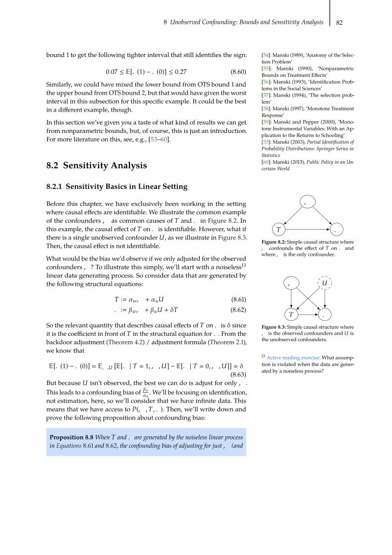
8 Unobserved Confounding: Bounds and Sensitivity Analysis 82
,
) .
Figure 8.2: Simple causal structure where
, confounds the effect of ) on . and
where, is the only confounder.
, *
) .
Figure 8.3: Simple causal structure where
, is the observed confounders and* is
the unobserved confounders.
13Active reading exercise: What assump-
tion is violated when the data are gener-
ated by a noiseless process?
bound 1 to get the following tighter interval that still identifies the sign:
0.07 ≤ E[.(1) − .(0)] ≤ 0.27 (8.60)
Similarly, we could have mixed the lower bound from OTS bound 1 and
the upper bound from OTS bound 2, but that would have given the worst
interval in this subsection for this specific example. It could be the best
in a different example, though.
In this section we’ve given you a taste of what kind of results we can get
from nonparametric bounds, but, of course, this is just an introduction.
For more literature on this, see, e.g., [53–60]
[54]: Manski (1989), ‘Anatomy of the Selec-
tion Problem’
[55]: Manski (1990), ‘Nonparametric
Bounds on Treatment Effects’
[56]: Manski (1993), ‘Identification Prob-
lems in the Social Sciences’
[57]: Manski (1994), ‘The selection prob-
lem’
[58]: Manski (1997), ‘Monotone Treatment
Response’
[59]: Manski and Pepper (2000), ‘Mono-
tone Instrumental Variables: With an Ap-
plication to the Returns to Schooling’
[53]: Manski (2003), Partial Identification ofProbability Distributions: Springer Series inStatistics[60]: Manski (2013), Public Policy in an Un-certain World
.
8.2 Sensitivity Analysis
8.2.1 Sensitivity Basics in Linear Setting
Before this chapter, we have exclusively been working in the setting
where causal effects are identifiable. We illustrate the common example
of the confounders, as common causes of ) and . in Figure 8.2. In
this example, the causal effect of ) on . is identifiable. However, what if
there is a single unobserved confounder* , as we illustrate in Figure 8.3.
Then, the causal effect is not identifiable.
What would be the bias we’d observe if we only adjusted for the observed
confounders,? To illustrate this simply, we’ll start with a noiseless13
linear data generating process. So consider data that are generated by
the following structural equations:
) := F, + D* (8.61)
. := �F, + �D* + �) (8.62)
So the relevant quantity that describes causal effects of ) on . is � since
it is the coefficient in front of ) in the structural equation for .. From the
backdoor adjustment (Theorem 4.2) / adjustment formula (Theorem 2.1),
we know that
E[.(1) − .(0)] = E,,* [E[. | ) = 1,,,*] − E[. | ) = 0,,,*]] = �(8.63)
But because * isn’t observed, the best we can do is adjust for only, .
This leads to a confounding bias of
�D D
. We’ll be focusing on identification,
not estimation, here, so we’ll consider that we have infinite data. This
means that we have access to %(,,), .). Then, we’ll write down and
prove the following proposition about confounding bias:
Proposition 8.8 When ) and . are generated by the noiseless linear processin Equations 8.61 and 8.62, the confounding bias of adjusting for just, (and

8 Unobserved Confounding: Bounds and Sensitivity Analysis 83
14Active reading exercise: Show that
E,,* [E[. | ) = 1,,,*] − E[. | ) = 0,,,*]]equals �.
. := �F, + �D* + �) (8.62 revisited)
not*) is �D D. Mathematically:
E, [E[. | ) = 1,,] − E[. | ) = 0,,]]
− E,,* [E[. | ) = 1,,,*] − E[. | ) = 0,,,*]] =�D D(8.64)
Proof. We’ll prove Proposition 8.8 in 3 steps:
1. Get a closed-form expression for E, [E[. | ) = C ,,]] in terms of
F , D , �F , and �D .2. Use step 1 to get a closed-form expression for the difference
E, [E[. | ) = 1,,] − E[. | ) = 0,,]].3. Subtract offE,,* [E[. | ) = 1,,,*] − E[. | ) = 0,,,*]] = �.14
First, we use the structural equation for . (Equation 8.62):
E, [E[. | ) = C ,,]] = E,[E[�F, + �D* + �) | ) = C ,,]
](8.65)
= E,[�F, + �DE[* | ) = C ,,] + �C
](8.66)
This is where we use the structural equation for ) (Equation 8.61). ) := F, + D* (8.61 revisited)
Rearranging it gives us * =)− F,
D. We can then use that for the
remaining conditional expectation:
= E,
[�F, + �D
(C − F,
D
)+ �C
](8.67)
= E,
[�F, +
�D DC −
�D F D
, + �C]
(8.68)
= �FE[,] +�D DC −
�D F D
E[,] + �C (8.69)
Then, rearranging a bit, we have the following:
=
(� +
�D D
)C +
(�F −
�D F D
)E[,] (8.70)
The only parts of this that matter are the parts that depend on C because
we want to know the effect of ) on .. For example, consider the expected
ATE estimate we would get if we were to only adjust for, :
E, [E[. | ) = 1,,] − E[. | ) = 0,,]] (8.71)
=
(� +
�D D
)(1) +
(�F −
�D F D
)E[,]
−[(� +
�D D
)(0) +
(�F −
�D F D
)E[,]
](8.72)
= � +�D D
(8.73)

8 Unobserved Confounding: Bounds and Sensitivity Analysis 84
, *
) .
Figure 8.4: Simple causal structure where
, is the observed confounders and* is
the unobserved confounders.
[61]: Cinelli et al. (2019), ‘Sensitivity Anal-
ysis of Linear Structural Causal Models’
15Recall Equation 8.73:
E, [E[. | ) = 1,,] − E[. | ) = 0,,]]
= � +�D D
(8.73 revisited)
Finally, subtracting off E,,* [E[. | ) = 1,,,*] − E[. | ) = 0,,,*]]:
Bias = E, [E[. | ) = 1,,] − E[. | ) = 0,,]]− E,,* [E[. | ) = 1,,,*] − E[. | ) = 0,,,*]] (8.74)
= � +�D D− � (8.75)
=�D D
(8.76)
Generalization toArbitraryGraphs/Estimands Here,we’veperformed
a sensitivity analysis for the ATE for the simple graph structure in Fig-
ure 8.4. For arbitrary estimands in arbitrary graphs, where the structural
equations are linear, see Cinelli et al. [61].
Sensitivity Contour Plots
Because Proposition 8.8 gives us a closed-form expression for the bias in
terms of the unobserved confounder parameters D and �D , we can plot
the levels of bias in contour plots. We show this in Figure 8.5a, where we
have1
Don the x-axis and �D on the y-axis.
If we rearrange Equation 8.7315to solve for �, we get the following:
� = E, [E[. | ) = 1,,] − E[. | ) = 0,,]] −�D D
(8.77)
So for given values of D and �D , we can compute the true ATE �,from the observational quantity E, [E[. | ) = 1,,] − E[. | ) = 0,,]].This allows us to get sensitivity curves that allow us to know how
robust conclusions like “E, [E[. | ) = 1,,] − E[. | ) = 0,,]] = 25 is
positive, so � is likely positive” are to unobserved confounding. We plot
such relevant contours of � in in Figure 8.5b.
15 10 5 0 5 10 1510.0
7.5
5.0
2.5
0.0
2.5
5.0
7.5
10.01102550
(a) Contours of confounding bias
�D D
0 1 2 3 4 5
0
20
40
60
80
10024150-25
(b) Contours of the true ATE �, given that
E, [E[. | ) = 1,,] − E[. | ) = 0,,]] = 25
.
Figure 8.5: Contour plots for sensitivity where the x-axis for both is1
Dand the y-axis is �D . There is a color-coded correspondence between
the curves in the upper right of Figure 8.5b and the curves in Figure 8.5

8 Unobserved Confounding: Bounds and Sensitivity Analysis 85
) := F, + D* (8.61 revisited)
[62]: RosenbaumandRubin (1983), ‘Assess-
ing Sensitivity to an Unobserved Binary
Covariate in an Observational Study with
Binary Outcome’
[63]: Imbens (2003), ‘Sensitivity to Exo-
geneity Assumptions in Program Evalua-
tion’
16Imbens [63] is the first to introduce con-
tour plots like the ones in our Figure 8.5.
[64]: Cinelli and Hazlett (2020), ‘Making
sense of sensitivity: extending omitted
variable bias’
[65]: Veitch and Zaveri (2020), Sense andSensitivity Analysis: Simple Post-Hoc Analy-sis of Bias Due to Unobserved Confounding
[66]: Liu et al. (2013), ‘An introduction to
sensitivity analysis for unobserved con-
founding in nonexperimental prevention
research’
[67]: Rosenbaum (2002), ObservationalStudies[68]: Rosenbaum (2010), Design of Observa-tional Studies[69]: Rosenbaum (2017), Observation andExperiment
[70]: Franks et al. (2019), ‘Flexible Sensi-
tivity Analysis for Observational Studies
Without Observable Implications’
[71]: Yadlowsky et al. (2020), Bounds on theconditional and average treatment effect withunobserved confounding factors[72]: Vanderweele and Arah (2011), ‘Bias
formulas for sensitivity analysis of unmea-
sured confounding for general outcomes,
treatments, and confounders’
[73]: Ding and VanderWeele (2016), ‘Sen-
sitivity Analysis Without Assumptions’
In the example we depict in Figure 8.5, the figure tells us that the green
curve (third from the bottom/left) indicates how strong the confounding
would need to be in order to completely explain the observed association.
In other words, ( 1
D, �D) would need be large enough to fall on the green
curve or above in order for the true ATE � to be zero or the opposite sign
of E, [E[. | ) = 1,,] − E[. | ) = 0,,]] = 25.
8.2.2 More General Settings
We consider a simple linear setting in Section 8.2.1 in order to easily
convey the important concepts in sensitivity analysis. However, there
is existing that allows us to do sensitivity analysis in more general
settings.
Say we are in the common setting where ) is binary. This is not the case
in the previous section (see Equation 8.61 ). Rosenbaum and Rubin [62]
and Imbens [63]16consider a simple binary treatment setting with binary
* by just putting a logistic sigmoid function around the right-hand side
of Equation 8.61 and using that for the probability of treatment instead
of the actual value of treatment:
%() = 1 | ,,*) :=1
1 + exp(−( F, + D*))(8.78)
No Assumptions on ) or * Fortunately, we can drop a lot of the
assumptions that we’ve seen so far. Unlike the linear form that we
assumed for ) in Section 8.2.1 and the linearish form that Rosenbaum
and Rubin [62] and Imbens [63] assume, Cinelli and Hazlett [64] develop
a method for sensitivity analysis that is agnostic to the functional form
of ). Their method also allows for* to be non-binary and for* to be a
vector, rather than just a single unobserved confounder.
Arbitrary Machine Learning Models for Parametrization of ) and .Recall that all of the estimators that we considered in Chapter 7 allowed
us to plug in arbitrary machine learning models to get model-assisted
estimators. Itmight be attractive to have an analogous option in sensitivity
analysis, potentially using the exact same models for the conditional
outcome model � and the propensity score 4 that we used for estimation.
And this is exactly what Veitch and Zaveri [65] give us. And they
are even able to derive a closed-form expression for confounding bias,
assuming the models we use for � and 4 are well-specified, something
that Rosenbaum and Rubin [62] and Imbens [63] didn’t do in their simple
setting.
Holy Shit; There Are a Lot of Options Although we only highlighted
a few options above, there are many different approaches to sensitivity
analysis, and people don’t agree on which ones are best. This means that
sensitivity analysis is an active area of current research. See Liu et al.
[66] for a review of methods that preceeded 2013. Rosenbaum is another
key figure in sensitivity analysis with his several different approaches
[67–69]. Here is a non-exhaustive list of a few other flexible sensitivity
analysis methods that you might be interested in looking into: Franks
et al. [70], Yadlowsky et al. [71], Vanderweele and Arah [72], and Ding
and VanderWeele [73].

Instrumental Variables 99.1 What is an Instrument? . . 869.2 No Nonparametric Identifi-
cation of the ATE . . . . . . 879.3 Warm-Up: Binary Linear Set-
ting . . . . . . . . . . . . . . . 879.4 Continuous Linear Setting 889.5 Nonparametric Identifica-
tion of Local ATE . . . . . . 90NewPotential NotationwithInstruments . . . . . . . . . 90
Principal Stratification . . . 90Local ATE . . . . . . . . . . . 91
9.6 More General Settings forATE Identification . . . . . 94
How can we identify causal effects when we are in the presence of
unobserved confounding?Onepopularway is to find anduse instrumentalvariables. An instrument (instrumental variable) / has three key qualities.
It affects on treatment ), it affects . only through ), and the effect of
/ on . is unconfounded. We depict these qualities in Figure 9.1. These
qualities allow us to use / to isolate the causal association flowing from
) to .. The intuition is that changes in / will be reflected in ) and lead
to corresponding changes in.. And these specifically /-focused changes
are unconfounded (unlike the changes to ) induced by the unobserved
confounder *), so they allow us to isolate the causal association that
flows from ) to ..
*
) .
/
Figure 9.1: Graph where* is an unobserved confounder of the effect of ) on . and / is an
instrumental variable.
9.1 What is an Instrument?
There are three main assumptions that must be satisfied for a variable /
to be considered an instrument. The first is that / must be relevant in
the sense that it must influence ).
Assumption 9.1 (Relevance) / has a causal effect on )
Graphically, the relevance assumption corresponds to the existence of an
active edge from / to ) in the causal graph. The second assumption is
known as the exclusion restriction.
Assumption 9.2 (Exclusion Restriction) / causal effect on . is fullymediated by )
This assumption is known as the exclusion restriction because it excludes
/ from the structural equation for . and from any other structural
equations that would make causal association flow from / to . without
going through ). Graphically, this means that we’ve excluded enough
potential edges between variables in the causal graph so that all causal
paths from / to . go through ). Finally, we assume that the causal effect
of / on . is unconfounded:

9 Instrumental Variables 87
*
) .
/
Figure 9.2: Graph where * is an unob-
served confounder of the effect of ) on .and / is an instrumental variable.
[18]: Pearl (2009), Causality
Assumption 9.3 (Instrumental Unconfoundedness) There are no back-door paths from / to ..
Conditional Instruments We phrased Assumption 9.3 as uncondi-
tional unconfoundedness, but all the math for instrumental variables still
works if we have unconfoundedness conditional on observed variables as
well. We just have to make sure we condition on those relevant variables.
In this case, you might see / referred to as a conditional instrument.
9.2 No Nonparametric Identification of the ATE
You might be wondering “if instrumental variables allow us to identify
causal effects, then why didn’t we see them back in Chapter 6 Non-
parametric Identification?” The answer is that instrumental variables
don’t nonparametrically identify the causal effect. We have nonparametric
identification when we don’t have to make any assumptions about the
parametric form.With instrumental variables,wemustmake assumptions
about the parametric form (e.g. linear) to identify causal effects.
We saw the following useful necessary condition for nonparametric
identification in Section 6.3: For each backdoor path from ) to any child
that is an ancestor of ., it is possible to block that path [18, p. 92]. And
we can see in Figure 9.2 that there is a backdoor path from ) to . that
cannot be blocked: ) ← * → .. So this necessary condition tells us that
we can’t use the instrument / to nonparametrically identify the effect of
) on ..
9.3 Warm-Up: Binary Linear Setting
As a warm-up, we’ll start in the setting where ) and / are binary and
where we make the parametric assumption that . is a linear function of
) and* :
Assumption 9.4 (Linear Outcome)
. := �) + D* (9.1)
The fact that / doesn’t appear in Equation 9.1 is a consequence of the
exclusion restriction (Assumption 9.2).
Then, with this assumption in mind, we’ll try to identify the causal effect
�. Because we have the intuition that / will be useful for identifying
the effect of ) on ., we’ll start with the associational difference for the
/-. relationship: E[. | / = 1] − E[. | / = 0]. By immediately applying
Assumption 9.4, we have the following:
E[. | / = 1] − E[. | / = 0] (9.2)
= E[�) + D* | / = 1] − E[�) + D* | / = 0] (9.3)

9 Instrumental Variables 88
[74]: Wald (1940), ‘The Fitting of Straight
Lines if Both Variables are Subject to Error’
Active reading exercise: Where did we use
each of Assumptions 9.1 to 9.4 in the above
derivation of Equation 9.7.
*
) .
/
�
I
Figure 9.3: Graph where * is an unob-
served confounder of the effect of ) on .and / is an instrumental variable.
Using linearity of expectation and rearranging a bit:
= � (E[) | / = 1] − E[) | / = 0]) + D (E[* | / = 1] − E[* | / = 0])(9.4)
Now, we use the instrumental unconfoundedness assumption (Assump-
tion 9.3). This means that / and* are independent, which allows us to
get rid of the* term:
= � (E[) | / = 1] − E[) | / = 0]) + D (E[*] − E[*]) (9.5)
= � (E[) | / = 1] − E[) | / = 0]) (9.6)
Then, we can solve for � to get the Wald estimand:
Proposition 9.1
� =E[. | / = 1] − E[. | / = 0]E[) | / = 1] − E[) | / = 0] (9.7)
Because of Assumption 9.1, we know that the denominator is non-zero,
so the right-hand side isn’t undefined. Then, we just plug in empirical
means in place of these conditional expectations to get the Wald estimator[74]:
� =
1
=1
∑8:I8=1
.8 − 1
=0
∑8:I8=0
.8
1
=1
∑8:I8=1
)8 − 1
=0
∑8:I8=0
)8(9.8)
where =1 is the number of samples where / = 1 and =0 is the number of
samples where / = 0.
Causal Effects as Multiplying Path Coefficients When the structural
equations are linear, you can think of the causal association flowing from
a variable � to a variable � as the product of the coefficients along the
directed path from � to �. If there are multiple paths, you just sum the
causal associations along all those paths. However, we don’t have direct
access to the causal association. Rather, we can measure total association,
and unblocked backdoor paths also contribute to total association, which
is why E[. | ) = 1] − E[. | ) = 0] ≠ �. So how can we identify the
effect of ) on . in Figure 9.3? Because there are no backdoor paths from
the instrument / to ., we can trivially identify the effect of / on .:
E[. | / = 1] − E[. | / = 0] = I�. Similarly, we can identify the effect
of the instrument on ): E[) | / = 1] − E[) | / = 0] = I . Then, we can
divide the effect of / on . by the effect of the / on ) to identify �( I� I
).
And this quotient is exactly the Wald estimand in Proposition 9.1.
9.4 Continuous Linear Setting
We’ll now consider the setting where ) and / are continuous, rather
than binary. We’ll still assume the linear form for . (Assumption 9.4),
which means that the causal efffect of ) on . is �. In the continuous
setting, we get the natural continuous analog of the Wald estimand:
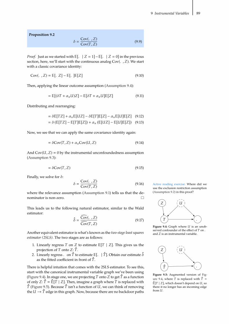
9 Instrumental Variables 89
Active reading exercise: Where did we
use the exclusion restriction assumption
(Assumption 9.2) in this proof?
*
) .
/
Figure 9.4: Graph where * is an unob-
served confounder of the effect of ) on .and / is an instrumental variable.
*
) .
/
Figure 9.5: Augmented version of Fig-
ure 9.4, where ) is replaced with ) =
E[) | /], which doesn’t depend on* , so
there it no longer has an incoming edge
from* .
Proposition 9.2
� =Cov(., /)Cov(), /) (9.9)
Proof. Just as we started with E[. | / = 1]−E[. | / = 0] in the previous
section, here, we’ll start with the continuous analog Cov(., /). We start
with a classic covariance identity:
Cov(., /) = E[./] − E[.]E[/] (9.10)
Then, applying the linear outcome assumption (Assumption 9.4):
= E[(�) + D*)/] − E[�) + D*]E[/] (9.11)
Distributing and rearranging:
= �E[)/] + DE[*/] − �E[)]E[/] − DE[*]E[/] (9.12)
= � (E[)/] − E[)]E[/]) + D (E[*/] − E[*]E[/]) (9.13)
Now, we see that we can apply the same covariance identity again:
= �Cov(), /) + DCov(*, /) (9.14)
And Cov(*, /) = 0 by the instrumental unconfoundedness assumption
(Assumption 9.3):
= �Cov(), /) (9.15)
Finally, we solve for �:
� =Cov(., /)Cov(), /) (9.16)
where the relevance assumption (Assumption 9.1) tells us that the de-
nominator is non-zero.
This leads us to the following natural estimator, similar to the Wald
estimator:
� =Cov(., /)Cov(), /)
(9.17)
Another equivalent estimator is what’s known as the two-stage least squaresestimator (2SLS). The two stages are as follows:
1. Linearly regress ) on / to estimate E[) | /]. This gives us the
projection of ) onto /: ).
2. Linearly regress . on ) to estimate E[. | )]. Obtain our estimate �as the fitted coefficient in front of ).
There is helpful intuition that comes with the 2SLS estimator. To see this,
start with the canonical instrumental variable graph we’ve been using
(Figure 9.4). In stage one, we are projecting ) onto / to get ) as a function
of only /: ) = E[) | /]. Then, imagine a graph where ) is replaced with
) (Figure 9.5). Because ) isn’t a function of* , we can think of removing
the* → ) edge in this graph. Now, because there are no backdoor paths

9 Instrumental Variables 90
[7]: Hernán and Robins (2020), Causal In-ference: What If
from ) to ., we can get that association is causation in stage two, where
we simply regress . on ) to estimate the causal effect. Note: We can also
use 2SLS in the binary setting we discussed in Section 9.3.
9.5 Nonparametric Identification of Local ATE
The problemwith the previous two sections is that we’vemade the strong
parametric assumption of linearity (Assumption 9.4). For example, this
assumption requires homogeneity (that the treatment effect is the same
for every unit). There are other variants that encode the homogeneity
assumption (see, e.g., Hernán and Robins [7, Section 16.3]), and they
are all strong assumptions. Ideally, we’d be able to use instrumental
variables for identification without making any parametric assumptions
such as linearity or homogeneity. And we can. We just need to settle for
a more specific causal estimand than the ATE and swap the linearity
assumption out for a new assumption. We will do this in the binary
setting, so both ) and / are binary. Before we can do that, we must define
a bit of new notation in Section 9.5.1 and introduce principal stratification
in Section 9.5.2.
9.5.1 New Potential Notation with Instruments
Just like we use .(1) , .() = 1) to denote the potential outcome we
would observe if we were to take treatment and .(0) , .() = 0) todenote the potential outcome we would observe if we were to not take
treatment, we will define similar potential notation with instruments.
We’ll think of the instrument / as encouragement for the treatment, so if
we have / = 1, we’re encouraged to take the treatment, and if we have
/ = 0, we’re encouraged to not take the treatment. Let )(1) , )(/ = 1)denote the treatment we would take if we were to get instrument value 1.
Similarly, let )(0) , )(/ = 0) denote the treatment we would take if we
were to get instrument value .
Then, we have the same for potential outcomes where we’re intervening
on the instrument, rather than the treatment: .(/ = 1) denotes the
outcome we would observe if we were to be encouraged to take the
treatment and .(/ = 0) denotes the outcome we would observe if we
were to be encouraged to not take the treatment.
9.5.2 Principal Stratification
We will segment the population into four principal strata, based on the
relationship between the encouragement / and the treatment taken ).
There are four strata because there is one for each combination of the
values the binary variables / and ) can take on.
Definition 9.1 (Principal Strata)
1. Compliers - always take the treatment that they’re encouraged to take.Namely, )(1) = 1 and )(0) = 0.

9 Instrumental Variables 91
*
) .
/
Figure 9.6:Causal graph for the compliers
and defiers.
*
) .
/
Figure 9.7: Causal graph for the always-
takers and never-takers.
2. Always-takers - always take the treatment, regardless of encouragement.Namely, )(1) = 1 and )(0) = 1.
3. Never-takers - never take the treatment, regardless of encouragement.Namely, )(1) = 0 and )(0) = 0.
4. Defiers - always take the opposite treatment of the treatment that theyare encouraged to take. Namely, )(1) = 0 and )(0) = 1.
Different CausalGraphs Importantly, these strata have different causal
graphs. While the treatment that the compliers and defiers take depends
on the encouragement (instrument), the treatment that the always-takers
and never-takers take does not. Therefore, the compliers and defiers
have the normal causal graph (Figure 9.6), whereas the always-takers
and never-takers have the same causal graph but with the /→ ) edge
removed (Figure 9.7). This means that the causal effect of / on ) is
zero for always-takers and never-takers. Then, because of the exclusion
restriction, this means that the causal effect of / on . is zero for the
always-takers and never-takers. This will be important for the upcoming
derivation.
Can’t Identify Stratum Given some observed value of/ and), we can’t
actually identify which stratum we’re in. There are four combinations of
the binary variables / and ); for each of these combinations, we’ll note
thatmore than one stratum is compatiblewith the observed combinations
of values.
1. / = 0, ) = 0. Compatible strata: compliers or never-takers
2. / = 0, ) = 1. Compatible strata: defiers or always-takers
3. / = 1, ) = 0. Compatible strata: defiers or never-takers
4. / = 1, ) = 1. Compatible strata: compliers or always-takers
Active reading exercise: Ensure that you
follow why these are the compatible strata
for each of these combinations of observed
values.
This means that we can’t identify if a given unit is a complier, a defier, an
always-taker, or a never-taker.
9.5.3 Local ATE
Although we won’t be able to use instrumental variables to nonpara-
metrically identify the ATE in the presence of unobserved confounding
(Section 9.2), we will be able to nonparametrically identify what’s known
as the local ATE. The local average treatment effect (LATE) is also known
as the complier average causal effect (CACE), as it is the ATE among the
compliers.
Definition 9.2 (Local Average Treatment Effect (LATE) / Complier
Average Causal Effect (CACE))
E[.() = 1) − .() = 0) | )(/ = 1) = 1, )(/ = 0) = 0] (9.18)
To identify the LATE, although we will no longer need the linearity as-
sumption (Assumption 9.4), we will need to introduce a new assumption
known as monotonicity.
Assumption 9.5 (Monotonicity)
∀8 , )8(/ = 1) ≥ )8(/ = 0) (9.19)

9 Instrumental Variables 92
Monotonicity means that if we are encouraged to take the treatment
(/ = 1), we are either more likely or equally likely to take the treatment
thanwewould be if wewere encouraged to not take the treatment (/ = 0).
Importantly, this means that we are assuming that there are no defiers.
This is because the compliers satisfy )(1) > )(0), the always-takers
and never-takers satisfy )(1) = )(0), but the defiers don’t satisfy either
of these; among the defiers, )(1) < )(0), which is a violation of the
monotonicity assumption.
Compliers: )(1) = 1, )(0) = 0
Always-takers: )(1) = 1, )(0) = 1
Never-takers: )(1) = 0, )(0) = 0
Defiers: )(1) = 0, )(0) = 1
We’ve now introduced the key concepts of principal strata and the
monotonicity assumption. Importantly, we saw that the causal effect of /
on . is zero among the always-takers and never-takers (Section 9.5.2),
and we just saw that monotonicity assumption implies that there are no
defiers. With this in mind, we are now ready to derive the nonparametric
identification result for the LATE estimand.
Theorem 9.3 (LATE Nonparametric Identification) Given that / is aninstrument, / and ) are binary variables, and that monotonicity holds, thefollowing is true:
E[.(1) − .(0) | )(1) = 1, )(0) = 0] = E[. | / = 1] − E[. | / = 0]E[) | / = 1] − E[) | / = 0]
(9.20)
Proof. Because we’re interested in the causal effect of ) on. and because
know that we’ll use the instrument /, we’ll start with the causal effect of
/ on . and decompose it into weighted stratum-specific causal effects
using the law of total probability:
E[.(/ = 1) − .(/ = 0)]= E[.(/ = 1) − .(/ = 0) | )(1) = 1, )(0) = 0]%()(1) = 1, )(0) = 0)+ E[.(/ = 1) − .(/ = 0) | )(1) = 0, )(0) = 1]%()(1) = 0, )(0) = 1)+ E[.(/ = 1) − .(/ = 0) | )(1) = 1, )(0) = 1]%()(1) = 1, )(0) = 1)+ E[.(/ = 1) − .(/ = 0) | )(1) = 0, )(0) = 0]%()(1) = 0, )(0) = 0)
(9.21)
The first term correponds to the compliers, the second term corresponds
to the the defiers, the third term corresponds to the always-takers, and the
last term corresponds to the never takers. Aswe discussed in Section 9.5.2,
the causal effect of / on . among the always-takers and never-takers is
zero, so we can remove those terms.
= E[.(/ = 1) − .(/ = 0) | )(1) = 1, )(0) = 0]%()(1) = 1, )(0) = 0)+ E[.(/ = 1) − .(/ = 0) | )(1) = 0, )(0) = 1]%()(1) = 0, )(0) = 1)
(9.22)
Because we’ve made the monotonicity assumption, we know that there
are no defiers (%()(1) = 0, )(0) = 1) = 0), so the defiers term is also zero.
= E[.(/ = 1) − .(/ = 0) | )(1) = 1, )(0) = 0]%()(1) = 1, )(0) = 0)(9.23)
Now, if we solve for this effect of / on . among the compliers, we get

9 Instrumental Variables 93
the following:
E[.(/ = 1) − .(/ = 0) | )(1) = 1, )(0) = 0] = E[.(/ = 1) − .(/ = 0)]%()(1) = 1, )(0) = 0)
(9.24)
And because these are the compliers, people who will take whichever
treatment they are encouraged to take, .(/ = 1) and .(/ = 0) are reallyequal to .() = 1) and .() = 0), respectively, so we can change the
left-hand side of Equation 9.24 to the LATE, the causal estimand that
we’re trying to identify:
E[.() = 1) − .() = 0) | )(1) = 1, )(0) = 0] (9.25)
=E[.(/ = 1) − .(/ = 0)]%()(1) = 1, )(0) = 0) (9.26)
Now, we apply the the instrumental unconfoundedness assumption
(Assumption 9.3) to identify the numerator.
=E[. | / = 1] − E[. | / = 0]
%()(1) = 1, )(0) = 0) (9.27)
All that’s left is to identify the denominator, the probability of being a
complier. However, we mentioned that we can’t identify the compliers in
Section 9.5.2, so how can we do this? This is where we’ll need to be a bit
clever. We’ll get this probability by taking everyone (probability 1) and
subtracting out the the always-takers and the compliers, since there are
no defiers, due to monotonicity (Assumption 9.5).
=E[. | / = 1] − E[. | / = 0]
1 − %() = 0 | / = 1) − %() = 1 | / = 0) (9.28)
To understand how we got the above equality, consider that everyone
either has / = 1 or / = 0. We can subtract out all of the never-takers
by removing those that had ) = 0 among the / = 1 subpopulation
(%() = 0 | / = 1)). Similarly, we can subtract out all of the always-takers
by removing those that had ) = 1 among the / = 0 subpopulation
(%() = 1 | / = 0)). We know that this removes all of the never-takers
and always-takers because there are no defiers and because we’ve looked
at both the / = 1 subpopulation and the / = 0 subpopulation. Now, we
just do a bit of manipulation:
=E[. | / = 1] − E[. | / = 0]
1 − (1 − %() = 1 | / = 1)) − %() = 1 | / = 0)(9.29)
=E[. | / = 1] − E[. | / = 0]
%() = 1 | / = 1) − %() = 1 | / = 0) (9.30)
Finally, because ) is a binary variable, we can swap out probabilities of
) = 1 for expectations:
=E[. | / = 1] − E[. | / = 0]E[) | / = 1] − E[) | / = 0] (9.31)

9 Instrumental Variables 94
[75]: Hartford et al. (2017), ‘Deep IV: A
Flexible Approach for Counterfactual Pre-
diction’
[76]: Xu et al. (2020), Learning Deep Featuresin Instrumental Variable Regression
[18]: Pearl (2009), Causality
[77]: Kilbertus et al. (2020), A Class of Al-gorithms for General Instrumental VariableModels
This is exactly the Wald estimand that we saw back in the linear setting
(Section 9.3) in Equation 9.7. However, this time, it is the corresponding
statistical estimand of the local ATE E[.() = 1) − .() = 0) | )(1) =1, )(0) = 0], also knownas the complier average causal effect (CACE). This
LATE/CACE causal estimand is in contrast to the ATE causal estimand
that we saw in Section 9.3: E[.() = 1) − .() = 0)]. The difference
is that the complier average causal effect is the ATE specifically in the
subpopulation of compliers, rather than the total population. It’s local(LATE) to that subpopulation, rather than being global over the whole
population like the ATE is. So we’ve seen two different assumptions that
get us to the Wald estimand with instrumental variables:
1. Linearity (or more generally homogeneity)
2. Monotonicity
Problems with LATE/CACE There are a few problems with the Wald
estimand for LATE, though. The first is that monotonicity might not be
satisfied in your setting of interest. The second is that, even ifmonotonicity
is satisfied, you might not be interested in the causal effect specifically
among the compliers, especially because you can’t even identify who the
compliers are (see Section 9.5.2). Rather, the regular ATE is often a more
useful quantity to know.
9.6 More General Settings for ATEIdentification
A common more general setting instrumental variable setting is to
consider that the outcome is generated by a complex function of treatment
and observed covariates plus some additive unobserved confounders:
. := 5 (),,) +* (9.32)
See, for example, Hartford et al. [75] and Xu et al. [76] for using deep
learning to model 5 . See references in those papers for using other
models such as kernel methods to model 5 . In those models and given
that * enters in the structural equation for . additively, you can get
identification with instrumental variables.
Alternatively, we could give up on point identification of causal effects,
instead settle for set identification (partial identification), and use instru-
mental variables to get bounds on causal effects. For more on that, see
Pearl [18, Section 8.2]. Additionally, settling for identifying a set, rather
than a point, allows us to relax the additive noise assumption above in
Equation 9.32. For example, Kilbertus et al. [77] considers the setting
where* doesn’t enter the structural equation for . additively:
. := 5 (),*) (9.33)
Difference in Differences 1010.1 Preliminaries . . . . . . . . . 9510.2 Introducing Time . . . . . . 9610.3 Identification . . . . . . . . . 96
Assumptions . . . . . . . . . 96Main Result and Proof . . . 97
10.4 Major Problems . . . . . . . 98
Note: the following chapter is muchmore rough than usual and currently
does not contain as many figures and intuition as the corresponding
lecture.
10.1 Preliminaries
We first introduced the unconfoundedness assumption (Assumption 2.1)
in Chapter 2:
(.(1), .(0)) ⊥⊥ ) (10.1)
Recall that this is equivalent to assuming that there are no unblocked
backdoor paths from ) to . in the causal graph. When this is the case,
we have that association is causation. In other words, it gives us the
following (hopefully familiar) identification of the ATE:
E[.(1) − .(0)] = E[.(1)] − E[.(0)] (10.2)
= E[.(1) | ) = 1] − E[.(0) | ) = 0] (10.3)
= E[. | ) = 1] − E[. | ) = 0] (10.4)
where we used this unconfoundedness in Equation 10.3.
However, the ATE is not the only average causal effect that we might be
interested in. It is often the case that practioners are interested in the ATE
specifically in the treated subpopulation. This is known as the averagetreatment effect on the treated (ATT): E[.(1) −.(0) | ) = 1]. We can make a
weaker assumption if we are only interested in the ATT, rather than the
ATE:
.(0) ⊥⊥ ) (10.5)
We only have to assume that .(0) is unconfounded here, rather than that
both .(0) and .(1) are unconfounded. We show this in the following
proof:
E[.(1) − .(0) | ) = 1] = E[.(1) | ) = 1] − E[.(0) | ) = 1] (10.6)
= E[. | ) = 1] − E[.(0) | ) = 1] (10.7)
= E[. | ) = 1] − E[.(0) | ) = 0] (10.8)
= E[. | ) = 1] − E[. | ) = 0] (10.9)
where we used this weaker unconfoundedness in Equation 10.8.
We are generally interested in the ATT estimand with difference-in-
differences, but we will use a different identifying assumption.

10 Difference in Differences 96
10.2 Introducing Time
We will now introduce the time dimension. Using information from the
time dimension will be key for us to get identification without assuming
the usual unconfoundedness. We’ll use � for the variable for time.
Setting As usual, we have a treatment group () = 1) and a control
group () = 0). However, now there is also time, and the treatment group
only gets the treatment after a certain time. So we have some time � = 1
that denotes a time after the treatment has been administered to the
treatment group and some time � = 0 that denotes some time before
the treatment has been administered to the treatment group. Because
the control group never gets the treatment, the control group hasn’t
received treatment at either of time � = 0 or at time � = 1. We will denote
the random variable for potential outcome under treatment C at time
� as .�(C). Then, the causal estimand we’re interested in is the average
difference in potential outcomes after treatment has been administered
(in time period � = 1) in the treatment group:
E[.1(1) − .1(0) | ) = 1] (10.10)
In other words, we’re interested in the ATT after the treatment has been
administered.
10.3 Identification
10.3.1 Assumptions
You can just treat .1 and .0 as two different random variables. So even
though we have a time subscript now, we still have trivial identification
via consistency (recall Assumption 2.5) when the value inside of the
parenthesis for the potential outcome matches the conditioning value for
):
Assumption 10.1 (Consistency) If the treatment is ), then the observedoutcome .� at time � is the potential outcome under treatment ). Formally,
∀�, ) = C =⇒ .� = .�(C) (10.11)
We could write this equivalently as follow:
∀�, .� = .�()) (10.12)
Consistency is what tells us that the causal estimand E[.�(1) | ) =
1] equals the statistical estimand E[.� | ) = 1], and, similarly, that
E[.�(0) | ) = 0] = E[.� | ) = 0]. In contrast, E[.�(1) | ) = 0] andE[.�(0) | ) = 1] are counterfactual causal estimands, so consistency does
not directly identify these quantities for us. Note: In our derivations
in this chapter, we are also implicitly assuming the no interference
assumption (Assumption 2.4) extended to this setting where we have a
time subscript.

10 Difference in Differences 97
Regular unconfoundedness:
.(0) ⊥⊥ ) (10.5 revisisted)
Wehavenowarrivedat thedefiningassumptionofdifference-in-differences:
parallel trends. This assumption states that the trend (over time) in the
treatment group would match the trend in the control group (over time)
if the treatment group were not given treatment.
Assumption 10.2 (Parallel Trends)
E[.1(0) − .0(0) | ) = 1] = E[.1(0) − .0(0) | ) = 0] (10.13)
This is like an assumption about unconfoundedness between difference:
(.1(0) − .0(0)) ⊥⊥ ) (10.14)
So you could see this as like the regular unconfoundedness we saw
in Equation 10.5, but where treatment is independent of a differenceof potential outcomes, rather than being independent of the potential
outcome themselves.
Then, we need one final assumption. This is the assumption that the
treatment has no effect on the treatment group before it is administered.
Assumption 10.3 (No Pretreatment Effect)
E[.0(1) − .0(0) | ) = 1] = 0 (10.15)
This assumptionmay seem like it’s obviously true, but that isn’t necessarily
the case. For example, if participants anticipate the treatment, then they
might be able to
10.3.2 Main Result and Proof
Using the assumptions in the previous section, we can show that the
ATT is equal to the difference between the differences across time in
each treatment group. We state this mathematically in the following
proposition.
Active reading exercise: How would you
estimate the statistical estimand on the
right-hand side of Equation 10.16?
Proposition 10.1 (Difference-in-differences Identification) Given consis-tency, parallel trends, and no pretreatment effect, we have the following:
E[.1(1) − .1(0) | ) = 1]= (E[.1 | ) = 1] − E[.0 | ) = 1]) − (E[.1 | ) = 0] − E[.0 | ) = 0])
(10.16)
Proof. As usual, we start with linearity of expectation:
E[.1(1) − .1(0) | ) = 1] = E[.1(1) | ) = 1] − E[.1(0) | ) = 1] (10.17)
We can immediately identify the treated potential outcome in the treated
group using consistency
= E[.1 | ) = 1] − E[.1(0) | ) = 1] (10.18)
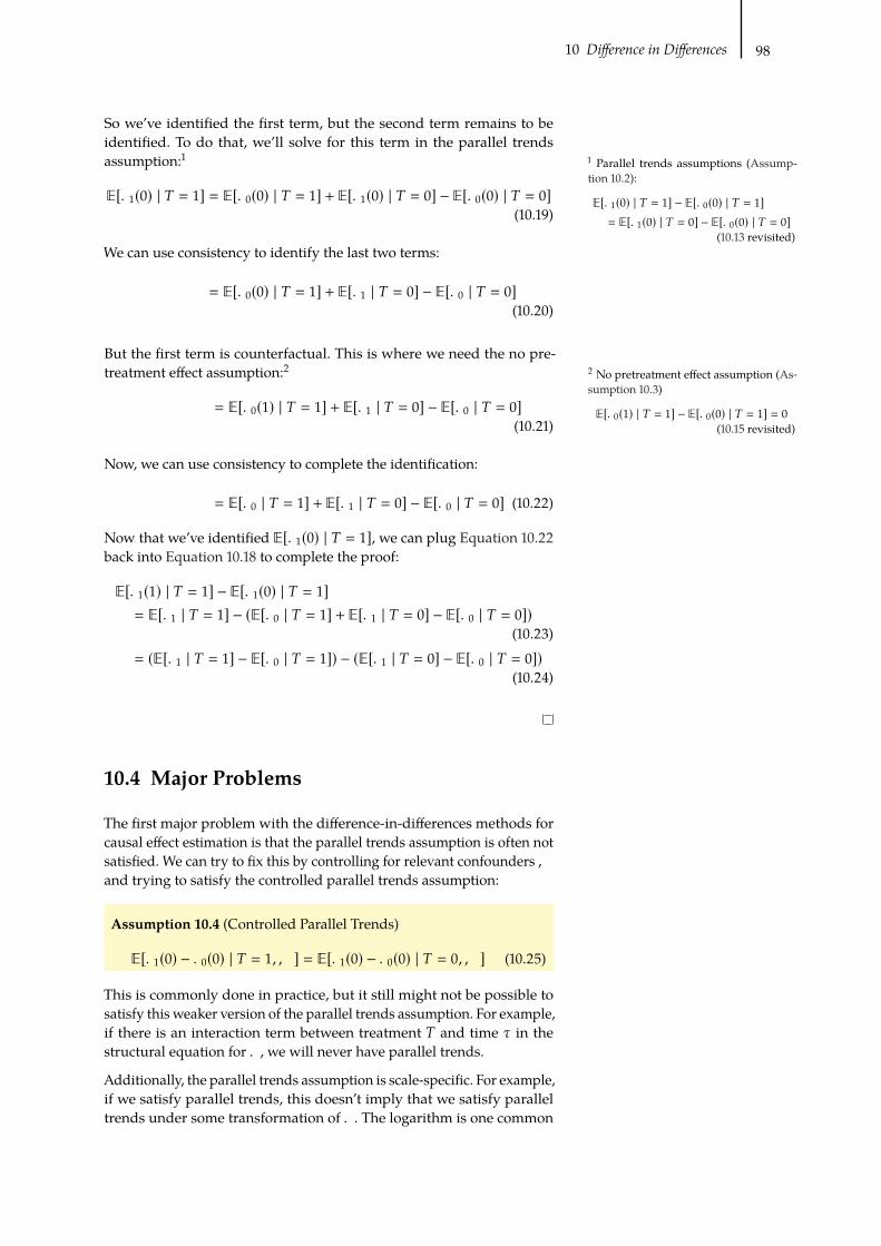
10 Difference in Differences 98
1Parallel trends assumptions (Assump-
tion 10.2):
E[.1(0) | ) = 1] − E[.0(0) | ) = 1]= E[.1(0) | ) = 0] − E[.0(0) | ) = 0]
(10.13 revisited)
2No pretreatment effect assumption (As-
sumption 10.3)
E[.0(1) | ) = 1] − E[.0(0) | ) = 1] = 0
(10.15 revisited)
So we’ve identified the first term, but the second term remains to be
identified. To do that, we’ll solve for this term in the parallel trends
assumption:1
E[.1(0) | ) = 1] = E[.0(0) | ) = 1] + E[.1(0) | ) = 0] − E[.0(0) | ) = 0](10.19)
We can use consistency to identify the last two terms:
= E[.0(0) | ) = 1] + E[.1 | ) = 0] − E[.0 | ) = 0](10.20)
But the first term is counterfactual. This is where we need the no pre-
treatment effect assumption:2
= E[.0(1) | ) = 1] + E[.1 | ) = 0] − E[.0 | ) = 0](10.21)
Now, we can use consistency to complete the identification:
= E[.0 | ) = 1] + E[.1 | ) = 0] − E[.0 | ) = 0] (10.22)
Now that we’ve identified E[.1(0) | ) = 1], we can plug Equation 10.22
back into Equation 10.18 to complete the proof:
E[.1(1) | ) = 1] − E[.1(0) | ) = 1]= E[.1 | ) = 1] − (E[.0 | ) = 1] + E[.1 | ) = 0] − E[.0 | ) = 0])
(10.23)
= (E[.1 | ) = 1] − E[.0 | ) = 1]) − (E[.1 | ) = 0] − E[.0 | ) = 0])(10.24)
10.4 Major Problems
The first major problem with the difference-in-differences methods for
causal effect estimation is that the parallel trends assumption is often not
satisfied. We can try to fix this by controlling for relevant confounders,
and trying to satisfy the controlled parallel trends assumption:
Assumption 10.4 (Controlled Parallel Trends)
E[.1(0) − .0(0) | ) = 1,,] = E[.1(0) − .0(0) | ) = 0,,] (10.25)
This is commonly done in practice, but it still might not be possible to
satisfy this weaker version of the parallel trends assumption. For example,
if there is an interaction term between treatment ) and time � in the
structural equation for ., we will never have parallel trends.
Additionally, the parallel trends assumption is scale-specific. For example,
if we satisfy parallel trends, this doesn’t imply that we satisfy parallel
trends under some transformation of .. The logarithm is one common

10 Difference in Differences 99
such transformation. This is because the parallel trends assumption
is an assumption about differences, which makes it not fully nonpara-
metric. In this sense, the parallel trends assumption is semi-parametric.
And, similarly, the difference-in-differences method is a semi-parametric
method.

�
� �
�
�
� �
Figure 11.1: Faithfulness counterexample
graph.
Causal Discovery fromObservational Data 11
11.1 Independence-Based CausalDiscovery . . . . . . . . . . 100
Assumptions and Theorem 100The PC Algorithm . . . . . . 102CanWe Get Any Better Iden-tification? . . . . . . . . . . . 104
11.2 Semi-Parametric Causal Dis-covery . . . . . . . . . . . . . 104
No Identifiability WithoutParametric Assumptions . 105
Linear Non-Gaussian Noise 105Nonlinear Models . . . . . . 108
11.3 Further Resources . . . . . . 109
Throughout this book, we have done causal inference, assumingwe know
the causal graph. What if we don’t know the graph? Can we learn it? As
you might expect, based on this being a running theme in this book, it
will depend on what assumptions we are willing to make. We will refer
to this problem as structure identification, which is distinct from the causal
estimand identification that we’ve seen in the book up until now.
11.1 Independence-Based Causal Discovery
11.1.1 Assumptions and Theorem
Themain assumption we’ve seen that relates the graph to the distribution
is theMarkov assumption. TheMarkov assumption tells us if variables are
d-separated in the graph �, then they are independent in the distribution
% (Theorem 3.1):
- ⊥⊥� . | / =⇒ - ⊥⊥% . | / (3.20 revisited)
Maybe we can detect independencies in the data and then use that
to infer the causal graph. However, going from independencies in the
distribution % to d-separations in the graph � isn’t something that the
Markov assumption gives us (see Equation 3.20 above). Rather, we need
the converse of the Markov assumption. This is known as the faithfulnessassumption.
Assumption 11.1 (Faithfulness)
- ⊥⊥� . | / ⇐= - ⊥⊥% . | / (11.1)
This assumption allows us to infer d-separations in the graph from
independencies in the distribution. Faithfulness, along with the Markov
assumption, actually implies minimality (Assumption 3.2), so it is a
stronger assumption. Faithfulness is a much less attractive assumption
than the Markov assumption because it is easy to think of counterexam-
ples (where two variables are independent in %, but there are unblocked
paths between them in �).
Faithfulness Counterexample Consider � and � in the causal graph
with coefficients in Figure 11.1. We have a violation of faithfulness when
the�→ �→ � path cancels out the�→ � → � path. To concretely see
how this could happen, consider the SCM that this graph represents:
� := � (11.2)
� := �� (11.3)
� := �� + �� (11.4)

11 Causal Discovery from Observational Data 101
-1
-2
-3
Figure 11.3: Immoralities are in their own
Markov equivalence class.
We can solve for the dependence between � and � by plugging in for �
and � in Equation 11.4 to get the following:
� = ( � + ��)� (11.5)
This means that the association flowing from � to � is � + �� in this
example. The two paths would cancel if � = −��, which would make
make � ⊥⊥ �. This violation of faithfulness would incorrectly lead us to
believe that there are no paths between � and � in the graph.
In addition to faithfulness, many methods also assume that there are no
unobserved confounders, which is known as causal sufficiency.
Assumption 11.2 (Causal Sufficiency) There are no unobserved con-founders of any of the variables in the graph.
Then, under the Markov, faithfulness, causal sufficiency, and acyclicity
assumptions, we can partially identify the causal graph. We can’t com-
pletely identify the causal graph because different graphs correspond
to the same set of independencies. For example, consider the graphs in
Figure 11.2.
-1 -2 -3
(a) Chain directed to the right
-1 -2 -3
(b) Chain directed to the left
-2
-1 -3
(c) Fork
Figure 11.2: Three Markov equivalent graphs
Although these are all distinct graphs, they correspond to the same set
of independence/dependence assumptions. Recall from Section 3.5 that
-1 ⊥⊥ -3 | -2 in distributions that areMarkovwith respect to any of these
three graphs in Figure 11.2. We also saw that minimality told us that -1
and-2 aredependent and that-2 and-3 aredependent.And the stronger
faithfulness assumption additionally tells us that in any distributions
that are faithful with respect to any of these graphs, -1 and -3 are
dependent if we don’t condition on -2. So using the presence/absence
of (conditional) independencies in the data isn’t enough to distinguish
these three graphs from each other; these graphs are Markov equivalent;
We say that two graphs are Markov equivalent if they correspond to
the same set of conditional independencies. Given a graph, we refer to
its Markov equivalence class as the set of graphs that encode the same
conditional independencies. Under faithfulness, we are able to identify a
graph from conditional independencies in the data if it is the only graph
in its Markov equivalence class. Any example of a graph that is the only
one in its Markov equivalence class the basic immorality that we show in
Figure 11.3. Recall from Section 3.6 that immoralities are distinct from
the two other basic graphical building blocks (chains and forks) in that
in Figure 11.3, -1 is (unconditionally) independent of -3, and -1 and -3
become dependent if we condition on -2. This means that while the basic
chains and fork in Figure 11.2 are in the same Markov equivalence class,
the basic immorality is by itself in its own Markov equivalence class.
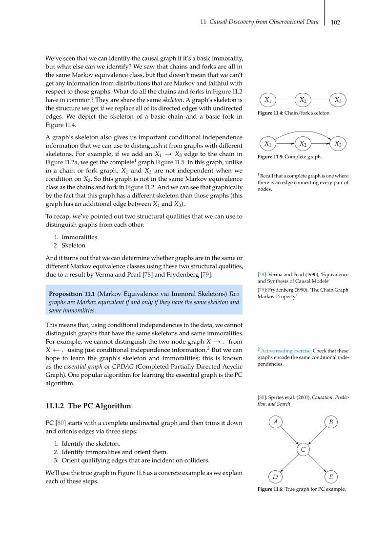
11 Causal Discovery from Observational Data 102
-1 -2 -3
Figure 11.5: Complete graph.
1Recall that a complete graph is onewhere
there is an edge connecting every pair of
nodes.
[78]: Verma and Pearl (1990), ‘Equivalence
and Synthesis of Causal Models’
[79]: Frydenberg (1990), ‘The Chain Graph
Markov Property’
2Active reading exercise: Check that these
graphs encode the same conditional inde-
pendencies.
[80]: Spirtes et al. (2001), Causation, Predic-tion, and Search
�
�
�
�
�
Figure 11.6: True graph for PC example.
-1 -2 -3
Figure 11.4: Chain/fork skeleton.
We’ve seen that we can identify the causal graph if it’s a basic immorality,
but what else can we identify? We saw that chains and forks are all in
the same Markov equivalence class, but that doesn’t mean that we can’t
get any information from distributions that are Markov and faithful with
respect to those graphs. What do all the chains and forks in Figure 11.2
have in common? They are share the same skeleton. A graph’s skeleton is
the structure we get if we replace all of its directed edges with undirected
edges. We depict the skeleton of a basic chain and a basic fork in
Figure 11.4.
A graph’s skeleton also gives us important conditional independence
information that we can use to distinguish it from graphs with different
skeletons. For example, if we add an -1 → -3 edge to the chain in
Figure 11.2a, we get the complete1graph Figure 11.5. In this graph, unlike
in a chain or fork graph, -1 and -3 are not independent when we
condition on -2. So this graph is not in the same Markov equivalence
class as the chains and fork in Figure 11.2. Andwe can see that graphically
by the fact that this graph has a different skeleton than those graphs (this
graph has an additional edge between -1 and -3).
To recap, we’ve pointed out two structural qualities that we can use to
distinguish graphs from each other:
1. Immoralities
2. Skeleton
And it turns out that we can determine whether graphs are in the same or
different Markov equivalence classes using these two structural qualities,
due to a result by Verma and Pearl [78] and Frydenberg [79]:
Proposition 11.1 (Markov Equivalence via Immoral Skeletons) Twographs are Markov equivalent if and only if they have the same skeleton andsame immoralities.
This means that, using conditional independencies in the data, we cannot
distinguish graphs that have the same skeletons and same immoralities.
For example, we cannot distinguish the two-node graph - → . from
- ← . using just conditional independence information.2But we can
hope to learn the graph’s skeleton and immoralities; this is known
as the essential graph or CPDAG (Completed Partially Directed Acyclic
Graph). One popular algorithm for learning the essential graph is the PC
algorithm.
11.1.2 The PC Algorithm
PC [80] starts with a complete undirected graph and then trims it down
and orients edges via three steps:
1. Identify the skeleton.
2. Identify immoralities and orient them.
3. Orient qualifying edges that are incident on colliders.
We’ll use the true graph in Figure 11.6 as a concrete example as we explain
each of these steps.

11 Causal Discovery from Observational Data 103
�
�
�
�
�
Figure 11.8: Graph from PC after we’ve
oriented the immoralities.
3This is called orientation propagation.
�
�
�
�
�
Figure 11.9: Graph from PC after we’ve
oriented edges that would form immoral-
ities if they were oriented in the other
(incorrect) direction.
Identify the Skeleton We discover the skeleton by starting with a
complete graph (Figure 11.7a) and then removing edges - − . where
- ⊥⊥ . | / for some (potentially empty) conditioning set /. So in our
example, we would start with the empty conditioning set and discover
that � ⊥⊥ � (since the only path from � to � in Figure 11.6 is blocked
by the collider �); this means we can remove the � − � edge, which
gives us the graph in Figure 11.7b. Then, we would move to conditioning
sets of size one and find that conditioning on � tells us that every other
pair of variables is conditionally independent given �, which allows
us to remove all edges that aren’t incident on �, resulting in the graph
in Figure 11.7c. And, indeed, this is the skeleton of the true graph in
Figure 11.6. More general PC would continue with larger conditioning
sets, to see if we can remove more edges, but conditioning sets of size
one are enough to discover the skeleton in this example.
�
�
�
�
�
(a) Complete undirected graph that we
start with
�
�
�
�
�
(b) Undirected graph that remains after
removing - − . edges where - ⊥⊥ .
�
�
�
�
�
(c) Undirected graph that remains after
removing - − . edges where - ⊥⊥ . | /
Figure 11.7: Illustration of the process of step 1 of PC, where we start with the complete graph (left) and remove edges until we’ve identified
the skeleton of the graph (right), given that the true graph is the one in Figure 11.6.
Identifying the Immoralities Now for any paths - − / − . in our
working graph where we discovered that there is no edge between - and
. in our previous step, if / was not in the conditioning set that makes
- and . conditionally independent, then we know - − / − . forms
an immorality. In other words, this means that - 6⊥⊥ . | /, which is a
property of an immorality that distinguishes it from chains and forks
(Section 3.6), so we can orient these edges to get - → / ← .. In our
example, this takes us from Figure 11.7c to Figure 11.8.
Orienting Qualifying Edges Incident on Colliders In the final step,
we take advantage of the fact that we might be able to orient more edges
since we know we discovered all of the immoralities in the previous step.
Any edge / −. part of a partially directed path of the form - → / −.,where there is no edge connecting - and ., can be oriented as /→ ..3
This is because if the true graph has the edge / ← ., we would have
found this in the previous step as that would have formed an immorality
- → /← .. Since we didn’t find that immorality in the previous step,
we know that the true direction is / → .. In our example, this means
we can orient the final two remaining edges, taking us from Figure 11.8
to Figure 11.9. It turns out that in this example, we are lucky that we
can orient all of the remaining edges in this last step, but this is not the
case in general. For example, we discussed that we wouldn’t be able
to distinguish simple chain graphs and simple fork graphs from each
other.

11 Causal Discovery from Observational Data 104
[80]: Spirtes et al. (2001), Causation, Predic-tion, and Search
[81]: Richardson (1996), ‘Feedback Models:
Interpretation and Discovery’
[82]: Hyttinen et al. (2013), ‘Discovering
Cyclic Causal Models with Latent Vari-
ables: A General SAT-Based Procedure’
[83]: Hyttinen et al. (2014), ‘Constraint-
Based Causal Discovery: Conflict Resolu-
tion with Answer Set Programming’
[84]: Shah and Peters (2020), ‘The hardness
of conditional independence testing and
the generalised covariance measure’
[85]: Meek (1995), ‘Strong Completeness
and Faithfulness in Bayesian Networks’
[86]: Geiger and Pearl (1988), ‘On the Logic
of Causal Models’
Dropping Assumptions There are algorithms that allow us to drop
various assumptions. The FCI (Fast Causal Inference) algorithm [80]
works without assuming causal sufficiency (Assumption 11.2). The CCD
algorithm [81] works without assuming acyclicity. And there is various
work on SAT-based causal discovery that allows us to drop both of the
above assumptions [82, 83].
Hardness of Conditional Independence Testing Allmethods that rely
on conditional independence tests such as PC, FCI, SAT-based algorithm,
etc. have an important practical issue associated with them. Conditional
independence tests are hard, and it can sometimes require a lot of data
to get accurate test results [84]. If we have infinite data, this isn’t an issue,
but we don’t have infinite data in practice.
11.1.3 Can We Get Any Better Identification?
We’ve seen that assuming the Markov assumption and faithfulness can
only get us so far; with those assumptions, we can only identify a graph
up to its Markov equivalence class. If we make more assumptions, can
we identify the graph more precisely than just its Markov equivalence
class?
Well, if we are in the case where the distributions are multinomial, we
cannot [85]. Or if we are in the common toy case where the SCMs are
linear with Gaussian noise, we cannot [86]. So we have the following
completeness result due to Geiger and Pearl [86] and Meek [85]:
Theorem 11.2 (Markov Completeness) If we have multinomial distribu-tions or linear Gaussian structural equations, we can only identify a graphup to its Markov equivalence class.
What if we don’t have multinomial distributions and don’t have linear
Gaussian SCMs, though?
11.2 Semi-Parametric Causal Discovery
In Theorem 11.2, we saw that, if we are in the linear Gaussian setting,
the best we can do is identify the Markov equivalence class; we cannot
hope to identify graphs that are in non-singleton Markov equivalence
classes. But what if we aren’t in the linear Gaussian setting? Can we
identify graphs if we are not in the linear Gaussian setting? We consider
the linear non-Gaussian noise setting in Section 11.2.2 and the nonlinearadditive noise setting in Section 11.2.3. It turns out that in both of these
settings, we can identify the causal graph. And we don’t have to assume
faithfulness (Assumption 11.1) in these settings.
By considering these settings, we are making semi-parametric assump-
tions (about functional form). If we don’t make any assumptions about
functional form, we cannot even identify the direction of the edge in a
two-node graph. We emphasize this in the next section before moving on
to the semi-parametric assumptions that allow us to identify the graph.

11 Causal Discovery from Observational Data 105
[14]: Peters et al. (2017), Elements of CausalInference: Foundations and Learning Algo-rithms
11.2.1 No Identifiability Without ParametricAssumptions
Markov Perspective Consider the two-variable setting, where the two
options of causal graphs are - → . and - ← .. Note that these
two graphs are Markov equivalent. Both don’t encode any conditional
independence assumptions, so both can describe arbitrary distributions
%(G, H). This means that conditional independencies in the data cannot
help us distinguish between - → . and - ← .. Using conditional
independencies, the bestwe cando is discover the corresponding essential
graph - − ..
SCMs Perspective How about if we consider this problem from the
perspective of SCMs; can we somehow distinguish - → . from - ← .
using SCMs? For an SCM, we want to write one variable as a function of
the other variable and some noise term variable. As you might expect,
if we don’t make any assumptions, there exist SCMs with the implied
causal graph - → . and SCMs with the implied causal graph - ← .
that both generate data according to %(G, H).
Proposition 11.3 (Non-Identifiability of Two-Node Graphs) For everyjoint distribution %(G, H) on two real-valued random variables, there is anSCM in either direction that generates data consistent with %(G, H).
Mathematically, there exists a function 5. such that
. = 5.(-,*.) , - ⊥⊥ *. (11.6)
and there exists a function 5- such that
- = 5-(.,*-) , . ⊥⊥ *- (11.7)
where*. and*- are real-valued random variables.
See, e.g., Peters et al. [14, p. 44] for a short proof. Similarly, this non-
identifiability result can be extended to more general graphs that have
more than two variables [see, e.g., 14, p. 135].
However, if we make assumptions about the parametric form of the
SCM, we can distinguish - → . from - ← . and identify graphs more
generally. That’s what we’ll see in the rest of this chapter.
11.2.2 Linear Non-Gaussian Noise
We saw in Theorem 11.2 that we cannot distinguish graphs within the
same Markov equivalence class if the structural equations are linear with
Gaussian noise* . For example, this means that we cannot distinguish
- → . from - ← .. However, if the noise term is non-Gaussian, then
we can identify the causal graph. As usual, we give this key assumption
of non-Gaussianity its own box:
Assumption 11.3 (Linear Non-Gaussian) All structural equations (causal

11 Causal Discovery from Observational Data 106
[87]: Darmois (1953), ‘Analyse générale des
liaisons stochastiques: etude particulière
de l’analyse factorielle linéaire’
[88]: Skitovich (1954), ‘Linear forms of in-
dependent random variables and the nor-
mal distribution law’
[88]: Skitovich (1954), ‘Linear forms of in-
dependent random variables and the nor-
mal distribution law’
mechanisms that generate the data) are of the following form:
. := 5 (-) +* (11.8)
where 5 is a linear function, - ⊥⊥ * , and* is distributed as a non-Gaussianrandom variable.
Then, in this linear non-Gaussian setting, we can identify which of
graphs - → . and - ← . is the true causal graph. We’ll first present
the theorem and proof and then get to the intuition.
Theorem 11.4 (Identifiability in Linear Non-Gaussian Setting) In thelinear non-Gaussian setting, if the true SCM is
. := 5 (-) +* , - ⊥⊥ * , (11.9)
then, there does not exist an SCM in the reverse direction
- := 6(.) + * , . ⊥⊥ * , (11.10)
that can generate data consistent with %(G, H).
Proof. We’ll first introduce a important result from Darmois [87] and
Skitovich [88] and Skitovich [88] that we’ll use to prove this theorem:
Theorem 11.5 (Darmois-Skitovich) Let -1 , . . . , -= be independent, non-degenerate random variables. If there exist coefficients 1 , . . . , = and�1 , . . . , �= that are all non-zero such that the two linear combinations
� = 1-1 + . . . + =-= and� = �1-1 + . . . + �=-=
are independent, then each -8 is normally distributed.
We will use the contrapositive of the special case of this theorem for
= = 2 to do almost all of the work for this proof:
Corollary 11.6 If either of the independent random variables -1 or -2 isnon-Gaussian, then there are no linear combinations
� = 1-1 + 2-2 and� = �1-1 + �2-2
such that � and � are independent (so � and � must be dependent).
Proof Outline With the above corollary in mind, our proof strategy is
to write . and * as linear combinations of - and* . By doing this, we
are effectively mapping our variables in Equations 11.9 and 11.10 onto the
variables in the corollary as follows:. onto�, * onto �,- onto-1, and*
onto-2. Then, we can apply the above corollary of the Darmois-Skitovich
Theorem to have that . and * must be dependent, which violates the
reverse direction SCM in Equation 11.10. We now proceed with the proof.

11 Causal Discovery from Observational Data 107
[89]: Shimizu et al. (2006), ‘A Linear Non-
Gaussian Acyclic Model for Causal Dis-
covery’
[14]: Peters et al. (2017), Elements of CausalInference: Foundations and Learning Algo-rithms
Forward model SCM:
. := 5 (-) +* , - ⊥⊥ *(11.9 revisited)
Backward model SCM:
- := 6(.) + * , . ⊥⊥ *(11.10 revisited)
We already have that we can write . as a linear combination of - and
* , since we’ve assumed the true structural equation in Equation 11.9 is
linear:
. = �- +* (11.11)
Then, to get * as a linear combination of - and* , we take the hypothe-
sized reverse SCM
- = �. + * (11.12)
from Equation 11.10, solve for * , and plug in Equation 11.11 for .:
* = - − �. (11.13)
= - − �(�- +*) (11.14)
= (1 − ��)- + �* (11.15)
Therefore, we’ve written both . and * as linear combinations of the
independent random variables - and* . This allows us to apply Corol-
lary 11.6 of the Darmois-Skitovish Theorem to get that . and * must be
dependent: . 6⊥⊥ * . This violates the reverse direction SCM:
- := 6(.) + * , . ⊥⊥ * (11.10 revisited)
We’ve given the proof here for just two variables, but it can be extended
to the more general setting with multiple variables (see [89] and [14,
Section 7.1.4]).
Graphical Intuition
When we fit the data in the causal direction, we get residuals that are
independent of the input variable, but when we fit the data in the
anti-causal direction, we get residuals that are dependent on the input
variable. We depict the regression line 5 we get if we linearly regress .
on - (causal direction) in Figure 11.10a, and we depict the regression
line 6 we get if we linearly regress - on . (anti-causal direction) in
Figure 11.10b. Just from these fits, you can see that the forward model (fit
in the causal direction) looks more pleasing than the backward model
(fit in the ant-causal direction).
To make this graphical intuition more clear, we plot the residuals of the
forward model 5 (causal direction) and the backward model 6 (anti-
causal direction) in Figure 11.11. The residuals in the forward direction
correspond to the following: * = . − 5 (-). And the residuals in the
backward direction correspond to the follow:ˆ* = - − 6(.). As you can
see in Figure 11.11a, the residuals of the forward model look independent
of the input variable - (on the x-axis). However in Figure 11.10b, the
residuals of the backward model don’t look independent of the input
variable . (on the x-axis) at all. Clearly, the range of the residuals (on the
vertical) changes as we move across values of . (from left to right).
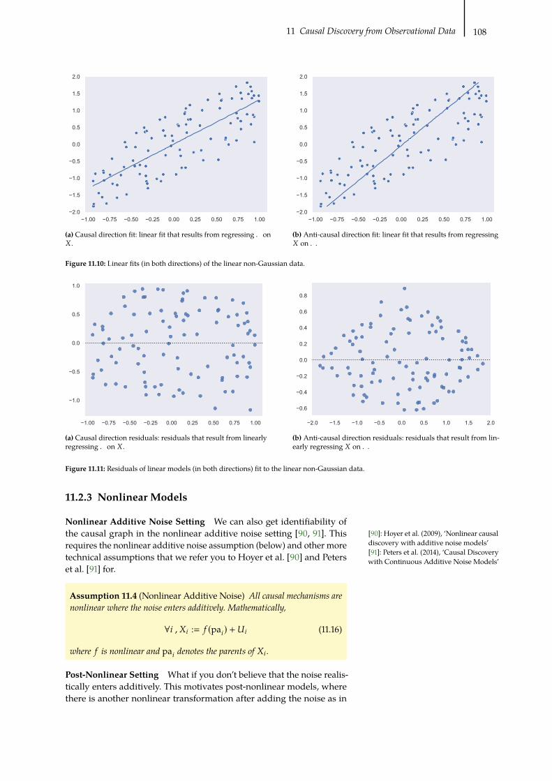
11 Causal Discovery from Observational Data 108
1.00 0.75 0.50 0.25 0.00 0.25 0.50 0.75 1.002.0
1.5
1.0
0.5
0.0
0.5
1.0
1.5
2.0
(a) Causal direction fit: linear fit that results from regressing . on
-.
1.00 0.75 0.50 0.25 0.00 0.25 0.50 0.75 1.002.0
1.5
1.0
0.5
0.0
0.5
1.0
1.5
2.0
(b) Anti-causal direction fit: linear fit that results from regressing
- on ..
Figure 11.10: Linear fits (in both directions) of the linear non-Gaussian data.
1.00 0.75 0.50 0.25 0.00 0.25 0.50 0.75 1.00
1.0
0.5
0.0
0.5
1.0
(a) Causal direction residuals: residuals that result from linearly
regressing . on -.
2.0 1.5 1.0 0.5 0.0 0.5 1.0 1.5 2.0
0.6
0.4
0.2
0.0
0.2
0.4
0.6
0.8
(b) Anti-causal direction residuals: residuals that result from lin-
early regressing - on ..
Figure 11.11: Residuals of linear models (in both directions) fit to the linear non-Gaussian data.
[90]: Hoyer et al. (2009), ‘Nonlinear causal
discovery with additive noise models’
[91]: Peters et al. (2014), ‘Causal Discovery
with Continuous Additive Noise Models’
11.2.3 Nonlinear Models
Nonlinear Additive Noise Setting We can also get identifiability of
the causal graph in the nonlinear additive noise setting [90, 91]. This
requires the nonlinear additive noise assumption (below) and other more
technical assumptions that we refer you to Hoyer et al. [90] and Peters
et al. [91] for.
Assumption 11.4 (Nonlinear Additive Noise) All causal mechanisms arenonlinear where the noise enters additively. Mathematically,
∀8 , -8 := 5 (pa8) +*8 (11.16)
where 5 is nonlinear and pa8 denotes the parents of -8 .
Post-Nonlinear Setting What if you don’t believe that the noise realis-
tically enters additively. This motivates post-nonlinear models, where
there is another nonlinear transformation after adding the noise as in

11 Causal Discovery from Observational Data 109
[92]: Zhang and Hyvärinen (2009), ‘On
the Identifiability of the Post-Nonlinear
Causal Model’
[93]: Eberhardt (2017), ‘Introduction to the
foundations of causal discovery’
[94]: Glymour et al. (2019), ‘Review of
Causal Discovery Methods Based on
Graphical Models’
[14]: Peters et al. (2017), Elements of CausalInference: Foundations and Learning Algo-rithms
Assumption 11.5 below. This setting can also yield identifiability (under
another technical condition). See Zhang and Hyvärinen [92] for more
details.
Assumption 11.5 (Post-Nonlinear)
∀8 , -8 := 6( 5 (pa8) +*8) (11.17)
where 5 is nonlinear and pa8 denotes the parents of -8 .
11.3 Further Resources
We conclude this chapter by pointing you to some relevant resources
for where to start learning more (in addition to the references in this
chapter). These references were also used as inspiration when forming
this chapter. See Eberhardt [93] and Glymour et al. [94] for two great
review articles from people at the frontier of causal discovery research.
And then if you want a whole book on this stuff, Peters et al. [14] wrote a
popular one!

Causal Discovery fromInterventional Data 12
12.1 Structural Interventions . . 110Single-Node Interventions 110Multi-Node Interventions . 110
12.2 Parametric Interventions . . 110Coming Soon . . . . . . . . . 110
12.3 Interventional MarkovEquivalence . . . . . . . . . 110
Coming Soon . . . . . . . . . 11012.4 Miscellaneous Other Set-
tings . . . . . . . . . . . . . . 110Coming Soon . . . . . . . . . 110
12.1 Structural Interventions
12.1.1 Single-Node Interventions
Coming Soon
12.1.2 Multi-Node Interventions
Coming Soon
12.2 Parametric Interventions
12.2.1 Coming Soon
12.3 Interventional Markov Equivalence
12.3.1 Coming Soon
12.4 Miscellaneous Other Settings
12.4.1 Coming Soon

Transfer Learning andTransportability 13
13.1 Causal Insights for TransferLearning . . . . . . . . . . . 111
Coming Soon . . . . . . . . . 11113.2 Transportability of Causal
Effects Across Populations 111Coming Soon . . . . . . . . . 111
13.1 Causal Insights for Transfer Learning
13.1.1 Coming Soon
13.2 Transportability of Causal Effects AcrossPopulations
13.2.1 Coming Soon

Counterfactuals and Mediation 1414.1 Counterfactuals Basics . . . 112
Coming Soon . . . . . . . . . 11214.2 Important Application: Me-
diation . . . . . . . . . . . . 112Coming Soon . . . . . . . . . 112
14.1 Counterfactuals Basics
14.1.1 Coming Soon
14.2 Important Application: Mediation
14.2.1 Coming Soon

Appendix

Proofs AA.1 Proof of Equation 6.1 from
Section 6.1 . . . . . . . . . . 114A.2 Proof of Propensity Score
Theorem (7.1) . . . . . . . . 114A.3 Proof of IPW Estimand (7.18)115
A.1 Proof of Equation 6.1 from Section 6.1
Claim Given the causal graph is Figure A.1, %(< | do(C)) = %(< | C).
,
") .
Figure A.1: Causal graph where, is un-
observed, sowe cannot block the backdoor
path ) ←, → ..
Proof. We first apply the Bayesian network factorization (Definition 3.1):
%(F, C, <, H) = %(F)%(C | F)%(< | C)%(H | F, <) (A.1)
Next, we apply the truncated factorization (Proposition 4.1):
%(F, <, H | do(C)) = %(F)%(< | C)%(H | F, <) (A.2)
Finally, we marginalize out F and H:∑F
∑H
%(F, <, H | do(C)) =∑F
∑H
%(F)%(< | C)%(H | F, <) (A.3)
%(< | do(C)) =(∑F
%(F))%(< | C)
(∑H
%(H | F, <))(A.4)
= %(< | C) (A.5)
A.2 Proof of Propensity Score Theorem (7.1)
Claim (.(1), .(0)) ⊥⊥ ) | , =⇒ (.(1), .(0)) ⊥⊥ ) | 4(,).
Proof. Assuming (.(1), .(0)) ⊥⊥ ) | , , we will prove (.(1), .(0)) ⊥⊥ ) |4(,) by showing that %() = 1, | .(C), 4(,)) does not depend on .(C),where .(C) is either potential outcome.
First, because ) is binary, can turn this probability into an expectation:
%() = 1, | .(C), 4(,)) = E[) | .(C), 4(,)] (A.6)
Then, using the law of iterated expectations, we can introduce, :
= E [E[) | .(C), 4(,),,] | .(C), 4(,)] (A.7)

A Proofs 115
Because we have now conditioned on all of, and 4(,) is a function of
, , it is redundant, so we can remove 4(,) from the inner expectation:
= E [E[) | .(C),,] | .(C), 4(,)] (A.8)
Now, we apply the unconfoundedness assumption we started with to
remove .(C) from the inner expectation:
= E [E[) | ,] | .(C), 4(,)] (A.9)
Again, using the fact that ) is binary, we can reduce the inner expectation
to %() = 1 | ,) , 4(,), something that is already conditioned on:
= E [%() = 1 | ,) | .(C), 4(,)] (A.10)
= E [4(,) | .(C), 4(,)] (A.11)
= 4(,) (A.12)
Because this does not depend on.(C), we’ve proven that) is independent
of .(C) given 4(,).
A.3 Proof of IPW Estimand (7.18)
Claim Underunconfoundedness andpositivity,E[.(C)] = E[1()=C).%(C |,)
].
Proof. We will start with the statistical estimand that we get from the ad-
justment formula (Theorem 2.1). Given unconfoundedness and positivity,
the adjustment formula tells us
E[.(C)] = E[E[. | C ,,]] (A.13)
We’ll assume the variable are discrete to break these expectations into
sums (replace with integrals if continuous):
=∑F
(∑H
H %(H | C , F))%(F) (A.14)
To get %(C | F) in there, we multiply by%(C |F)%(C |F) :
=∑F
∑H
H %(H | C , F)%(F) %(C | F)%(C | F) (A.15)
Then, noticing that %(H | C , F)%(C | F)%(F) is the joint distribution:
=∑F
∑H
H %(H, C, F) 1
%(C | F) (A.16)

A Proofs 116
∑H H %(H, C, F) is nearly
∑H H %(H) = E[.], but because of ) = C and
, = F are in the probability, the terms of this sum are only non-zero if
) = C and, = F. Therefore, we get the indicator random variable for
this event in the expectation that is over all three random variables (),
, , and .):
=∑F
E [1() = C ,, = F).] 1
%(C | F) (A.17)
Now, the
∑F
1
%(C |F) that remains is a weighted expectation over , .
Integrating this means that because we are nowmarginalizing over, , F
becomes a random variable (,) and the the, = F inside the indicator
becomes redundant. This gives us the following:
= E
[1() = C).%(C | ,)
](A.18)
Note: For some people, it might be more natural to skip straight from
Equation A.16 to Equation A.18.

Bibliography
Here are the references in citation order.
[1] Tyler Vigen. Spurious correlations. https://www.tylervigen.com/spurious-correlations. 2015(cited on page 3).
[2] Jerzy Splawa-Neyman. ‘On the Application of Probability Theory to Agricultural Experiments. Essay
on Principles. Section 9.’ Trans. by D. M. Dabrowska and T. P. Speed. In: Statistical Science 5.4 (1923
[1990]), pp. 465–472 (cited on page 6).
[3] Donald B. Rubin. ‘Estimating causal effects of treatments in randomized and nonrandomized studies.’
In: Journal of educational Psychology 66.5 (1974), p. 688 (cited on pages 6, 7).
[4] Jasjeet S. Sekhon. ‘The Neyman-Rubin Model of Causal Inference and Estimation via Matching
Methods’. In: Oxford handbook of political methodology (2008), pp. 271– (cited on page 6).
[5] Paul W. Holland. ‘Statistics and Causal Inference’. In: Journal of the American Statistical Association 81.396
(1986), pp. 945–960. doi: 10.1080/01621459.1986.10478354 (cited on pages 8, 42).
[6] Alexander D’Amour, Peng Ding, Avi Feller, Lihua Lei, and Jasjeet Sekhon. Overlap in ObservationalStudies with High-Dimensional Covariates. 2017 (cited on page 13).
[7] Miguel A Hernán and James M Robins. Causal Inference: What If. Boca Raton: Chapman & Hall/CRC,
2020 (cited on pages 14, 27, 90).
[8] Miguel Angel Luque-Fernandez, Michael Schomaker, Daniel Redondo-Sanchez, Maria Jose Sanchez
Perez, Anand Vaidya, and Mireille E Schnitzer. ‘Educational Note: Paradoxical collider effect in the
analysis of non-communicable disease epidemiological data: a reproducible illustration and web
application’. In: International Journal of Epidemiology 48.2 (Dec. 2018), pp. 640–653. doi: 10.1093/ije/
dyy275 (cited on pages 16, 45).
[9] Salim S. Virani et al. ‘Heart Disease and Stroke Statistics—2020 Update: A Report From the American
Heart Association’. In: Circulation (Mar. 2020), pp. 640–653. doi: 10.1161/cir.0000000000000757
(cited on page 16).
[10] Trevor Hastie, Robert Tibshirani, and Jerome Friedman. The Elements of Statistical Learning. SpringerSeries in Statistics. New York, NY, USA: Springer New York Inc., 2001 (cited on pages 17, 63).
[11] Dominik Janzing, David Balduzzi, Moritz Grosse-Wentrup, and Bernhard Schölkopf. ‘Quantifying
causal influences’. In: Ann. Statist. 41.5 (Oct. 2013), pp. 2324–2358. doi: 10.1214/13-AOS1145 (cited on
page 18).
[12] Stephen L. Morgan and Christopher Winship. Counterfactuals and Causal Inference: Methods and Principlesfor Social Research. 2nd ed. Analytical Methods for Social Research. Cambridge University Press, 2014
(cited on pages 18, 78).
[13] Daphne Koller and Nir Friedman. Probabilistic Graphical Models: Principles and Techniques. AdaptiveComputation and Machine Learning. The MIT Press, 2009 (cited on pages 21, 29, 47).
[14] J. Peters, D. Janzing, and B. Schölkopf. Elements of Causal Inference: Foundations and Learning Algorithms.Cambridge, MA, USA: MIT Press, 2017 (cited on pages 21, 105, 107, 109).
[15] Judea Pearl, Madelyn Glymour, and Nicholas P Jewell. Causal inference in statistics: A primer. John Wiley
& Sons, 2016 (cited on page 25).
[16] Judea Pearl. Probabilistic Reasoning in Intelligent Systems: Networks of Plausible Inference. San Francisco,
CA, USA: Morgan Kaufmann Publishers Inc., 1988 (cited on page 29).
[17] Judea Pearl. ‘Causal inference in statistics: An overview’. In: Statist. Surv. 3 (2009), pp. 96–146. doi:
10.1214/09-SS057 (cited on page 42).

[18] Judea Pearl. Causality. Cambridge University Press, 2009 (cited on pages 44, 47, 48, 59, 87, 94).
[19] Felix Elwert and Christopher Winship. ‘Endogenous Selection Bias: The Problem of Conditioning on a
Collider Variable.’ In: Annual review of sociology 40 (2014), pp. 31–53 (cited on page 44).
[20] David Galles and Judea Pearl. ‘An Axiomatic Characterization of Causal Counterfactuals’. In: Founda-tions of Science 3.1 (1998), pp. 151–182. doi: 10.1023/A:1009602825894 (cited on page 47).
[21] Joseph Y. Halpern. ‘Axiomatizing Causal Reasoning’. In: Proceedings of the Fourteenth Conference onUncertainty in Artificial Intelligence. UAI’98. Madison, Wisconsin: Morgan Kaufmann Publishers Inc.,
1998, pp. 202–210 (cited on page 47).
[22] Elizabeth L. Ogburn and Tyler J. VanderWeele. ‘Causal Diagrams for Interference’. In: Statist. Sci. 29.4(Nov. 2014), pp. 559–578. doi: 10.1214/14-STS501 (cited on page 48).
[23] J. Pearl. ‘On the consistency rule in causal inference: axiom, definition, assumption, or theorem?’ In:
Epidemiology 21.6 (Nov. 2010), pp. 872–875 (cited on page 48).
[24] Judea Pearl. ‘Causal diagrams for empirical research’. In: Biometrika 82.4 (Dec. 1995), pp. 669–688. doi:
10.1093/biomet/82.4.669 (cited on pages 55, 56).
[25] Ilya Shpitser and Judea Pearl. ‘Identification of Joint Interventional Distributions in Recursive Semi-
Markovian Causal Models’. In: Proceedings of the 21st National Conference on Artificial Intelligence - Volume2. AAAI’06. Boston, Massachusetts: AAAI Press, 2006, pp. 1219–1226 (cited on pages 57, 60).
[26] Yimin Huang and Marco Valtorta. ‘Pearl’s Calculus of Intervention is Complete’. In: Proceedings of theTwenty-Second Conference on Uncertainty in Artificial Intelligence. UAI’06. Cambridge, MA, USA: AUAI
Press, 2006, pp. 217–224 (cited on page 57).
[27] Jin Tian and Judea Pearl. ‘A General Identification Condition for Causal Effects’. In: Eighteenth NationalConference on Artificial Intelligence. Edmonton, Alberta, Canada: American Association for Artificial
Intelligence, 2002, pp. 567–573 (cited on page 59).
[28] Ilya Shpitser and Judea Pearl. ‘Identification of Conditional Interventional Distributions’. In: Proceedingsof the Twenty-Second Conference on Uncertainty in Artificial Intelligence. UAI’06. Cambridge, MA, USA:
AUAI Press, 2006, pp. 437–444 (cited on page 60).
[29] F. Pedregosa et al. ‘Scikit-learn: Machine Learning in Python’. In: Journal of Machine Learning Research12 (2011), pp. 2825–2830 (cited on pages 62, 64).
[30] SörenR.Künzel, Jasjeet S. Sekhon, Peter J. Bickel, andBinYu. ‘Metalearners for estimatingheterogeneous
treatment effects using machine learning’. In: Proceedings of the National Academy of Sciences 116.10 (2019),pp. 4156–4165. doi: 10.1073/pnas.1804597116 (cited on pages 64–67).
[31] Uri Shalit, Fredrik D. Johansson, and David Sontag. ‘Estimating individual treatment effect: general-
ization bounds and algorithms’. In: ed. by Doina Precup and Yee Whye Teh. Vol. 70. Proceedings of
Machine Learning Research. International Convention Centre, Sydney, Australia: PMLR, June 2017,
pp. 3076–3085 (cited on pages 65, 66).
[32] Paul R. Rosenbaum and Donald B. Rubin. ‘The central role of the propensity score in observational
studies for causal effects’. In: Biometrika 70.1 (Apr. 1983), pp. 41–55. doi: 10.1093/biomet/70.1.41
(cited on page 67).
[33] D. G. Horvitz and D. J. Thompson. ‘A Generalization of Sampling Without Replacement from a
Finite Universe’. In: Journal of the American Statistical Association 47.260 (1952), pp. 663–685. doi:
10.1080/01621459.1952.10483446 (cited on page 69).
[34] JasonAbrevaya, Yu-ChinHsu, andRobert P. Lieli. ‘EstimatingConditionalAverageTreatment Effects’. In:
Journal of Business & Economic Statistics 33.4 (2015), pp. 485–505. doi: 10.1080/07350015.2014.975555
(cited on page 70).
[35] Joseph D. Y. Kang and Joseph L. Schafer. ‘Demystifying Double Robustness: A Comparison of
Alternative Strategies for Estimating a Population Mean from Incomplete Data’. In: Statist. Sci. 22.4(Nov. 2007), pp. 523–539. doi: 10.1214/07-STS227 (cited on page 70).
[36] Paul N Zivich and Alexander Breskin.Machine learning for causal inference: on the use of cross-fit estimators.2020 (cited on page 70).

[37] Vincent Dorie, Jennifer Hill, Uri Shalit, Marc Scott, and Dan Cervone. ‘Automated versus Do-It-Yourself
Methods for Causal Inference: Lessons Learned from a Data Analysis Competition’. In: Statist. Sci. 34.1(Feb. 2019), pp. 43–68. doi: 10.1214/18-STS667 (cited on page 70).
[38] Shaun R. Seaman and Stijn Vansteelandt. ‘Introduction to Double Robust Methods for Incomplete
Data’. In: Statist. Sci. 33.2 (May 2018), pp. 184–197. doi: 10.1214/18-STS647 (cited on page 70).
[39] Anastasios Tsiatis. Semiparametric theory and missing data. Springer Science & Business Media, 2007
(cited on page 70).
[40] James M. Robins, Andrea Rotnitzky, and Lue Ping Zhao. ‘Estimation of Regression Coefficients When
Some Regressors are not Always Observed’. In: Journal of the American Statistical Association 89.427
(1994), pp. 846–866. doi: 10.1080/01621459.1994.10476818 (cited on page 70).
[41] Heejung Bang and James M. Robins. ‘Doubly Robust Estimation in Missing Data and Causal Inference
Models’. In: Biometrics 61.4 (2005), pp. 962–973. doi: 10.1111/j.1541-0420.2005.00377.x (cited on
page 70).
[42] Mark J Van Der Laan and Daniel Rubin. ‘Targeted maximum likelihood learning’. In: The internationaljournal of biostatistics 2.1 (2006) (cited on page 70).
[43] Megan S. Schuler and Sherri Rose. ‘Targeted Maximum Likelihood Estimation for Causal Inference in
Observational Studies’. In: American Journal of Epidemiology 185.1 (Jan. 2017), pp. 65–73. doi: 10.1093/
aje/kww165 (cited on page 70).
[44] Mark J Van der Laan and Sherri Rose. Targeted learning: causal inference for observational and experimentaldata. Springer Science & Business Media, 2011 (cited on page 70).
[45] Elizabeth A. Stuart. ‘Matching Methods for Causal Inference: A Review and a Look Forward’. In: Statist.Sci. 25.1 (Feb. 2010), pp. 1–21. doi: 10.1214/09-STS313 (cited on page 71).
[46] Victor Chernozhukov, Denis Chetverikov, Mert Demirer, Esther Duflo, Christian Hansen, Whitney
Newey, and JamesRobins. ‘Double/debiasedmachine learning for treatment and structural parameters’.
In: The Econometrics Journal 21.1 (2018), pp. C1–C68. doi: 10.1111/ectj.12097 (cited on page 71).
[47] Chris Felton. Chernozhukov et al. on Double / Debiased Machine Learning. https://scholar.princeton.edu/sites/default/files/bstewart/files/felton.chern_.slides.20190318.pdf. 2018 (cited
on page 71).
[48] Vasilis Syrgkanis. Orthogonal/Double Machine Learning. https://econml.azurewebsites.net/spec/estimation/dml.html. Accessed: 16 September 2020. 2019 (cited on page 71).
[49] Dylan J. Foster and Vasilis Syrgkanis. Orthogonal Statistical Learning. 2019 (cited on page 71).
[50] SusanAthey andGuido Imbens. ‘Recursive partitioning for heterogeneous causal effects’. In: Proceedingsof the National Academy of Sciences 113.27 (2016), pp. 7353–7360. doi: 10.1073/pnas.1510489113 (cited
on page 71).
[51] Stefan Wager and Susan Athey. ‘Estimation and Inference of Heterogeneous Treatment Effects using
Random Forests’. In: Journal of the American Statistical Association 113.523 (2018), pp. 1228–1242. doi:
10.1080/01621459.2017.1319839 (cited on page 71).
[52] Susan Athey, Julie Tibshirani, and Stefan Wager. ‘Generalized random forests’. In: Ann. Statist. 47.2(Apr. 2019), pp. 1148–1178. doi: 10.1214/18-AOS1709 (cited on page 71).
[53] Charles F. Manski. Partial Identification of Probability Distributions: Springer Series in Statistics. English.Springer, 2003 (cited on pages 73, 82).
[54] Charles Manski. ‘Anatomy of the Selection Problem’. In: Journal of Human Resources 24.3 (1989),
pp. 343–360 (cited on pages 73, 82).
[55] Charles F. Manski. ‘Nonparametric Bounds on Treatment Effects’. In: The American Economic Review80.2 (1990), pp. 319–323 (cited on pages 73, 74, 79–82).
[56] Charles F. Manski. ‘Identification Problems in the Social Sciences’. In: Sociological Methodology 23 (1993),
pp. 1–56 (cited on pages 73, 82).

[57] Charles F. Manski. ‘The selection problem’. In: Advances in Econometrics: Sixth World Congress. Ed. byChristopher A.Editor Sims. Vol. 1. Econometric Society Monographs. Cambridge University Press,
1994, pp. 143–170. doi: 10.1017/CCOL0521444594.004 (cited on pages 73, 82).
[58] Charles F. Manski. ‘Monotone Treatment Response’. In: Econometrica 65.6 (1997), pp. 1311–1334 (cited
on pages 73, 76, 82).
[59] Charles F. Manski and John V. Pepper. ‘Monotone Instrumental Variables: With an Application to the
Returns to Schooling’. In: Econometrica 68.4 (2000), pp. 997–1010 (cited on pages 73, 78, 82).
[60] Charles F. Manski. Public Policy in an Uncertain World. Harvard University Press, 2013 (cited on pages 73,
82).
[61] Carlos Cinelli, Daniel Kumor, Bryant Chen, Judea Pearl, and Elias Bareinboim. ‘Sensitivity Analysis
of Linear Structural Causal Models’. In: ed. by Kamalika Chaudhuri and Ruslan Salakhutdinov.
Vol. 97. Proceedings of Machine Learning Research. Long Beach, California, USA: PMLR, Sept. 2019,
pp. 1252–1261 (cited on page 84).
[62] P. R. Rosenbaum and D. B. Rubin. ‘Assessing Sensitivity to an Unobserved Binary Covariate in
an Observational Study with Binary Outcome’. In: Journal of the Royal Statistical Society. Series B(Methodological) 45.2 (1983), pp. 212–218 (cited on page 85).
[63] Guido W. Imbens. ‘Sensitivity to Exogeneity Assumptions in Program Evaluation’. In: AmericanEconomic Review 93.2 (May 2003), pp. 126–132. doi: 10.1257/000282803321946921 (cited on page 85).
[64] Carlos Cinelli and Chad Hazlett. ‘Making sense of sensitivity: extending omitted variable bias’.
In: Journal of the Royal Statistical Society: Series B (Statistical Methodology) 82.1 (2020), pp. 39–67. doi:
10.1111/rssb.12348 (cited on page 85).
[65] Victor Veitch and Anisha Zaveri. Sense and Sensitivity Analysis: Simple Post-Hoc Analysis of Bias Due toUnobserved Confounding. 2020 (cited on page 85).
[66] W. Liu, S. J. Kuramoto, and E. A. Stuart. ‘An introduction to sensitivity analysis for unobserved
confounding in nonexperimental prevention research’. In: Prev Sci 14.6 (Dec. 2013), pp. 570–580 (cited
on page 85).
[67] Paul Rosenbaum. Observational Studies. Jan. 2002 (cited on page 85).
[68] Paul R Rosenbaum. Design of Observational Studies. Vol. 10. Springer, 2010 (cited on page 85).
[69] Paul R Rosenbaum. Observation and Experiment. Harvard University Press, 2017 (cited on page 85).
[70] AlexanderM. Franks, Alexander D’Amour, and Avi Feller. ‘Flexible Sensitivity Analysis for Observa-
tional Studies Without Observable Implications’. In: Journal of the American Statistical Association 0.0
(2019), pp. 1–33. doi: 10.1080/01621459.2019.1604369 (cited on page 85).
[71] Steve Yadlowsky, Hongseok Namkoong, Sanjay Basu, John Duchi, and Lu Tian. Bounds on the conditionaland average treatment effect with unobserved confounding factors. 2020 (cited on page 85).
[72] T. J. Vanderweele and O. A. Arah. ‘Bias formulas for sensitivity analysis of unmeasured confounding
for general outcomes, treatments, and confounders’. In: Epidemiology 22.1 (Jan. 2011), pp. 42–52 (cited
on page 85).
[73] P. Ding and T. J. VanderWeele. ‘Sensitivity Analysis Without Assumptions’. In: Epidemiology 27.3 (May
2016), pp. 368–377 (cited on page 85).
[74] Abraham Wald. ‘The Fitting of Straight Lines if Both Variables are Subject to Error’. In: Ann. Math.Statist. 11.3 (Sept. 1940), pp. 284–300. doi: 10.1214/aoms/1177731868 (cited on page 88).
[75] Jason Hartford, Greg Lewis, Kevin Leyton-Brown, and Matt Taddy. ‘Deep IV: A Flexible Approach
for Counterfactual Prediction’. In: ed. by Doina Precup and Yee Whye Teh. Vol. 70. Proceedings of
Machine Learning Research. International Convention Centre, Sydney, Australia: PMLR, June 2017,
pp. 1414–1423 (cited on page 94).
[76] Liyuan Xu, Yutian Chen, Siddarth Srinivasan, Nando de Freitas, Arnaud Doucet, and Arthur Gretton.
Learning Deep Features in Instrumental Variable Regression. 2020 (cited on page 94).

[77] Niki Kilbertus, Matt J. Kusner, and Ricardo Silva. A Class of Algorithms for General Instrumental VariableModels. 2020 (cited on page 94).
[78] Thomas Verma and Judea Pearl. ‘Equivalence and Synthesis of Causal Models’. In: Proceedings of theSixth Annual Conference on Uncertainty in Artificial Intelligence. UAI ’90. USA: Elsevier Science Inc., 1990,
pp. 255–270 (cited on page 102).
[79] Morten Frydenberg. ‘The Chain Graph Markov Property’. In: Scandinavian Journal of Statistics 17.4(1990), pp. 333–353 (cited on page 102).
[80] Peter Spirtes, Clark Glymour, and Richard Scheines. Causation, Prediction, and Search. MIT Press, Jan.
2001 (cited on pages 102, 104).
[81] Thomas Richardson. ‘Feedback Models: Interpretation and Discovery’. PhD thesis. 1996 (cited on
page 104).
[82] Antti Hyttinen, Patrik O. Hoyer, Frederick Eberhardt, and Matti Järvisalo. ‘Discovering Cyclic Causal
Models with Latent Variables: A General SAT-Based Procedure’. In: Proceedings of the Twenty-NinthConference on Uncertainty in Artificial Intelligence. UAI’13. Bellevue, WA: AUAI Press, 2013, pp. 301–310
(cited on page 104).
[83] Antti Hyttinen, Frederick Eberhardt, and Matti Järvisalo. ‘Constraint-Based Causal Discovery: Conflict
Resolution with Answer Set Programming’. In: Proceedings of the Thirtieth Conference on Uncertainty inArtificial Intelligence. UAI’14. Quebec City, Quebec, Canada: AUAI Press, 2014, pp. 340–349 (cited on
page 104).
[84] Rajen D. Shah and Jonas Peters. ‘The hardness of conditional independence testing and the generalised
covariance measure’. In: Ann. Statist. 48.3 (June 2020), pp. 1514–1538. doi: 10.1214/19-AOS1857 (cited
on page 104).
[85] Christopher Meek. ‘Strong Completeness and Faithfulness in Bayesian Networks’. In: Proceedings ofthe Eleventh Conference on Uncertainty in Artificial Intelligence. UAI’95. Montréal, Qué, Canada: Morgan
Kaufmann Publishers Inc., 1995, pp. 411–418 (cited on page 104).
[86] Dan Geiger and Judea Pearl. ‘On the Logic of Causal Models’. In: Proceedings of the Fourth AnnualConference on Uncertainty in Artificial Intelligence. UAI ’88. NLD: North-Holland Publishing Co., 1988,
pp. 3–14 (cited on page 104).
[87] G. Darmois. ‘Analyse générale des liaisons stochastiques: etude particulière de l’analyse factorielle
linéaire’. In: Revue de l’Institut International de Statistique / Review of the International Statistical Institute21.1/2 (1953), pp. 2–8 (cited on page 106).
[88] V. P. Skitovich. ‘Linear forms of independent random variables and the normal distribution law’. In:
Izvestiia Akademii Nauk SSSR, Serija Matematiceskie 18 (1954), pp. 185–200 (cited on page 106).
[89] Shohei Shimizu, Patrik O. Hoyer, Aapo Hyvärinen, and Antti Kerminen. ‘A Linear Non-Gaussian
Acyclic Model for Causal Discovery’. In: Journal of Machine Learning Research 7.72 (2006), pp. 2003–2030
(cited on page 107).
[90] Patrik Hoyer, Dominik Janzing, Joris MMooij, Jonas Peters, and Bernhard Schölkopf. ‘Nonlinear causal
discovery with additive noise models’. In: Advances in Neural Information Processing Systems. Ed. byD. Koller, D. Schuurmans, Y. Bengio, and L. Bottou. Vol. 21. Curran Associates, Inc., 2009, pp. 689–696
(cited on page 108).
[91] Jonas Peters, Joris M. Mooij, Dominik Janzing, and Bernhard Schölkopf. ‘Causal Discovery with
Continuous Additive Noise Models’. In: Journal of Machine Learning Research 15.58 (2014), pp. 2009–2053(cited on page 108).
[92] Kun Zhang and Aapo Hyvärinen. ‘On the Identifiability of the Post-Nonlinear Causal Model’. In:
Proceedings of the Twenty-Fifth Conference on Uncertainty in Artificial Intelligence. UAI ’09. Montreal,
Quebec, Canada: AUAI Press, 2009, pp. 647–655 (cited on page 109).
[93] Frederick Eberhardt. ‘Introduction to the foundations of causal discovery’. In: International Journal ofData Science and Analytics 3.2 (2017), pp. 81–91. doi: 10.1007/s41060-016-0038-6 (cited on page 109).

[94] Clark Glymour, Kun Zhang, and Peter Spirtes. ‘Review of Causal Discovery Methods Based on
Graphical Models’. In: Frontiers in Genetics 10 (2019), p. 524. doi: 10.3389/fgene.2019.00524 (cited on
page 109).

Alphabetical Index
2SLS, 89
adjustment formula, 11
ancestor, 19
association, 4
causal association, 4, 30
confounding association,
4, 30
associational difference, 8
ATT, 95
average treatment effect (ATE),
8, 62
backdoor adjustment, 38
backdoor criterion, 37
backdoor path, 37
Bayesian network, 21
chain rule, 21
factorization, 21
Berkson’s paradox, 27
blocked path, 25, 26, 28
causal Bayesian networks,
35
causal effect
average, 8, 62
complier average, 91
conditional average, 62
individual, 7, 62
individualized average,
62
unit-level, 7
causal estimand, 15, 33
causal forests, 71
causal graph, 22
non-strict, 23
strict, 22
causal mechanism, 34, 41
causal sufficiency, 101
causal tree, 71
cause, 22, 41
child, 19
collider, 26
collider bias, 43
COM estimator, 63
common cause, 4
common support, 13
comparability, 49
complier average causal effect
(CACE), 91
conditional average treatment
effect (CATE), 62
conditional instrument, 87
conditional outcome model,
63
confounder, 4
consistent, 70
correlation, 4
counterfactual, 8
covariate balance, 49
CPDAG, 102
curse of dimensionality, 13
cycle, 19
d-connected, 29
d-separated, 29
d-separation, 29
data generating process, 27
descendant, 19
direct cause, 22, 41
directed acyclic graph (DAG),
19
directed graph, 19
directed path, 19
do-calculus, 55do-operator, 32double robustness, 70
doubly robust, 70
edge, 19
endogenous, 41
Equationtown, 53
essential graph, 102
estimand, 15
causal, 15, 33
statistical, 15, 33
estimate, 15
estimation, 15, 16
estimator, 15
exchangeability, 9, 50
exogenous, 41
extrapolation, 13
factual, 8
faithfulness, 100
frontdoor adjustment, 53
frontdoor criterion, 53
generalized random forests,
71
global Markov assumption,
29
graph, 19
hedge criterion, 60
homogeneity, 90
identifiability, 10, 33
identification, 10, 16, 33
nonparametric, 57
parametric, 57, 63
structure, 100
ignorability, 9
immorality, 20, 26
individual treatment effect
(ITE), 7, 62
individualized average
treatment effect
(IATE), 62
instrument, 86
conditional, 87
instrumental variable, 86
interference, 13
interventional distribution,
32
interventional SCM, 42
inverse probability weighting,
68
IPW, 68
local average treatment effect
(LATE), 91
local Markov assumption,
20
lurking variable, 4
M-bias, 44, 47
magnification, 43
magnify, 43
manipulated graph, 34, 55
Markov compatibility, 21
Markov equivalence, 101
Markovian, 41
mediator, 43
minimality, 21
misspecification, 18
model-assisted estimation,
16

model-assisted estimator, 16,
17
monotone treatment response
(MTR), 76
monotonicity, 91
no-assumptions bound, 75
node, 19
non-Markovian, 41
nonparametric, 40
nonparametric identification,
57
observational data, 33
observational distribution,
33
observational-counterfactual
decomposition, 75
optimal treatment selection
(OTS), 79
orientation propagation, 103
overlap, 13
parallel trends, 96
parametric identification, 57,
63
parent, 19
path, 19
blocked, 25, 26
blocked , 28
unblocked, 25, 27
unblocked , 28
positivity, 12
post-intervention, 33
post-treatment covariates,
44
potential outcome, 6
pre-intervention, 33
propensity score, 67
pseudo-populations, 68
randomized control trials
(RCTs), 49
randomized experiments,
49
semi-Markovian, 41
Simpson’s paradox, 1
skeleton, 102
spurious correlation, 3
statistical estimand, 15, 33
structural causal model (SCM),
40
structural equation, 40
structure identification, 100
sufficient adjustment set, 38
SUTVA, 14
targeted maximum likelihood
estimation, 70
TARNet, 65
terminology machine gun,
19
TMLE, 70
treatment assignment
mechanism, 49
truncated factorization, 35
two-stage least squares, 89
unblocked path, 25, 27, 28
unconfounded children
criterion, 59
unconfoundedness, 11
undirected graph, 19
unit-level treatment effect, 7
vertex, 19
Wald Estimand, 88
Wald estimator, 88
X-learner, 66