Embed Size (px)
Citation preview
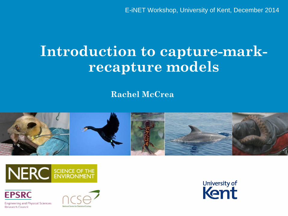
Introduction to capture-mark-recapture models
E-iNET Workshop, University of Kent, December 2014
Rachel McCrea
Overview
• Introduction
• Lincoln-Petersen estimate
• Maximum-likelihood theory*
• Capture-mark-recapture
• Cormack-Jolly-Seber model
• Developments
* Technical aside
Historical Context
• Estimation of the population of France (1802)
• Human demography What are we interested in?
• Marking of birds started ~1899 in Denmark
• Capture-recapture techniques widely applied: Medical Epidemiological Sociological Ecological
Lincoln-Petersen Estimate
• Two sample experiment
• Interested in estimating population size, N
Lincoln-Petersen Estimate
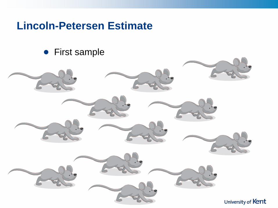
• First sample
Lincoln-Petersen Estimate
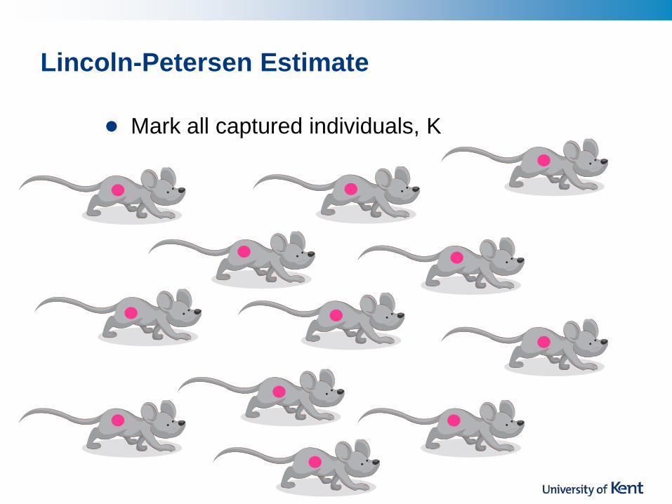
• Mark all captured individuals, K
Lincoln-Petersen Estimate
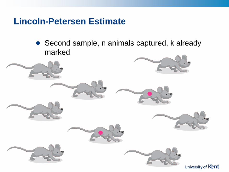
• Second sample, n animals captured, k already marked
Lincoln-Petersen Estimate
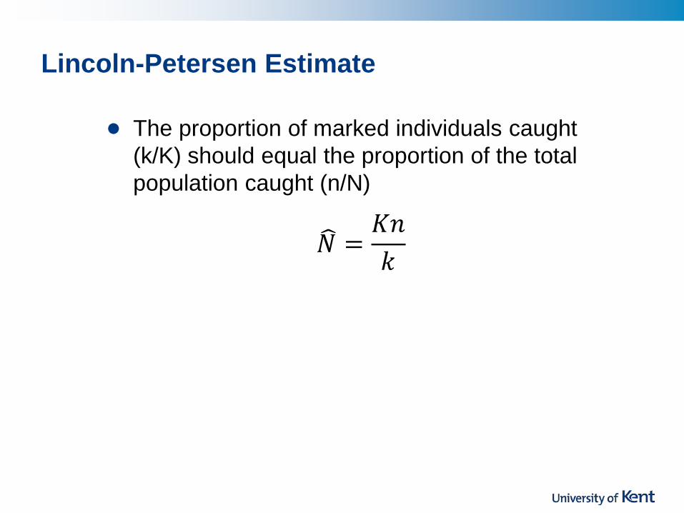
• The proportion of marked individuals caught (k/K) should equal the proportion of the total population caught (n/N)
𝑁� =𝐾𝐾𝑘
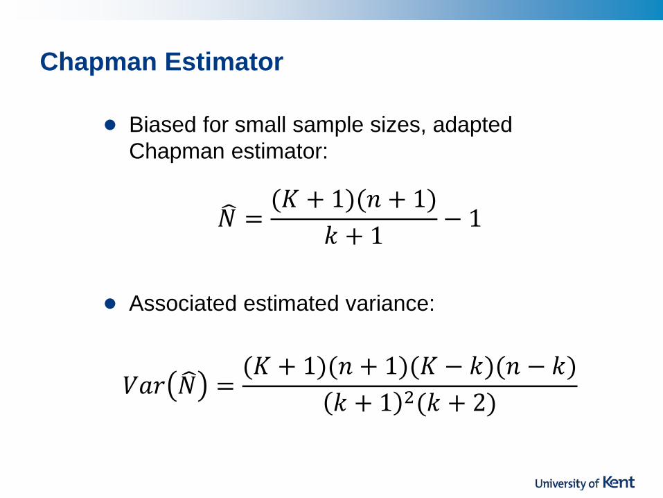
Chapman Estimator
• Biased for small sample sizes, adapted Chapman estimator:
𝑁� =(𝐾 + 1)(𝐾 + 1)
𝑘 + 1− 1
• Associated estimated variance:
𝑉𝑉𝑉 𝑁� =(𝐾 + 1)(𝐾 + 1)(𝐾 − 𝑘)(𝐾 − 𝑘)
𝑘 + 1 2(𝑘 + 2)
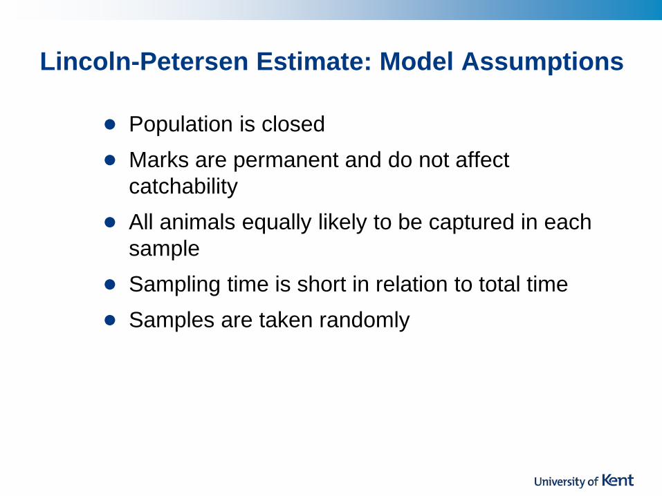
Lincoln-Petersen Estimate: Model Assumptions
• Population is closed
• Marks are permanent and do not affect catchability
• All animals equally likely to be captured in each sample
• Sampling time is short in relation to total time
• Samples are taken randomly
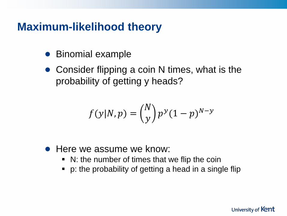
Maximum-likelihood theory
• Binomial example
• Consider flipping a coin N times, what is the probability of getting y heads?
𝑓(𝑦|𝑁,𝑝) = 𝑁𝑦 𝑝𝑦(1 − 𝑝)𝑁−𝑦
• Here we assume we know: N: the number of times that we flip the coin p: the probability of getting a head in a single flip
Maximum-likelihood theory
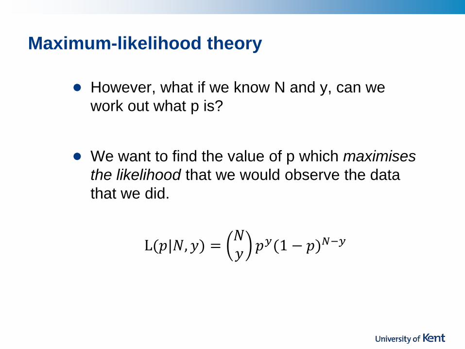
• However, what if we know N and y, can we work out what p is?
• We want to find the value of p which maximises the likelihood that we would observe the data that we did.
L(𝑝|𝑁,𝑦) = 𝑁𝑦 𝑝𝑦(1 − 𝑝)𝑁−𝑦
Maximum-likelihood theory
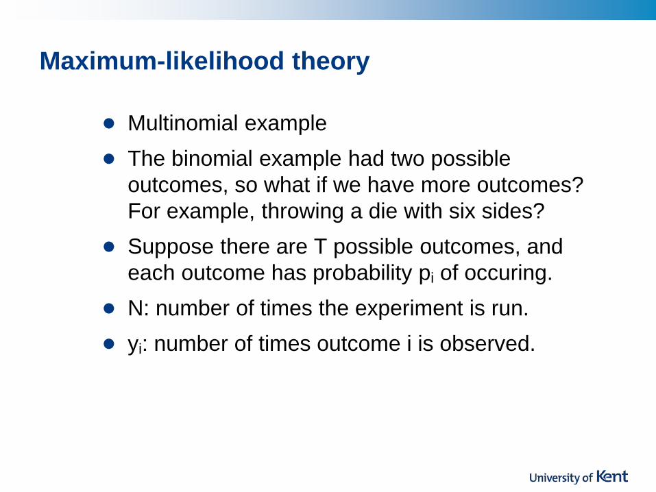
• Multinomial example
• The binomial example had two possible outcomes, so what if we have more outcomes? For example, throwing a die with six sides?
• Suppose there are T possible outcomes, and each outcome has probability pi of occuring.
• N: number of times the experiment is run.
• yi: number of times outcome i is observed.
Maximum-likelihood theory
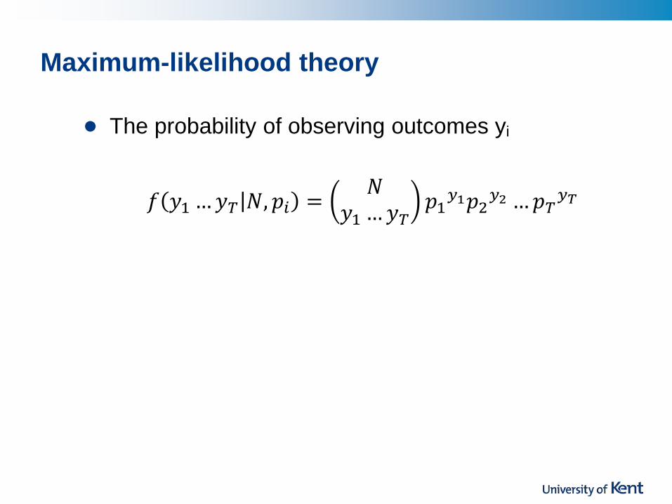
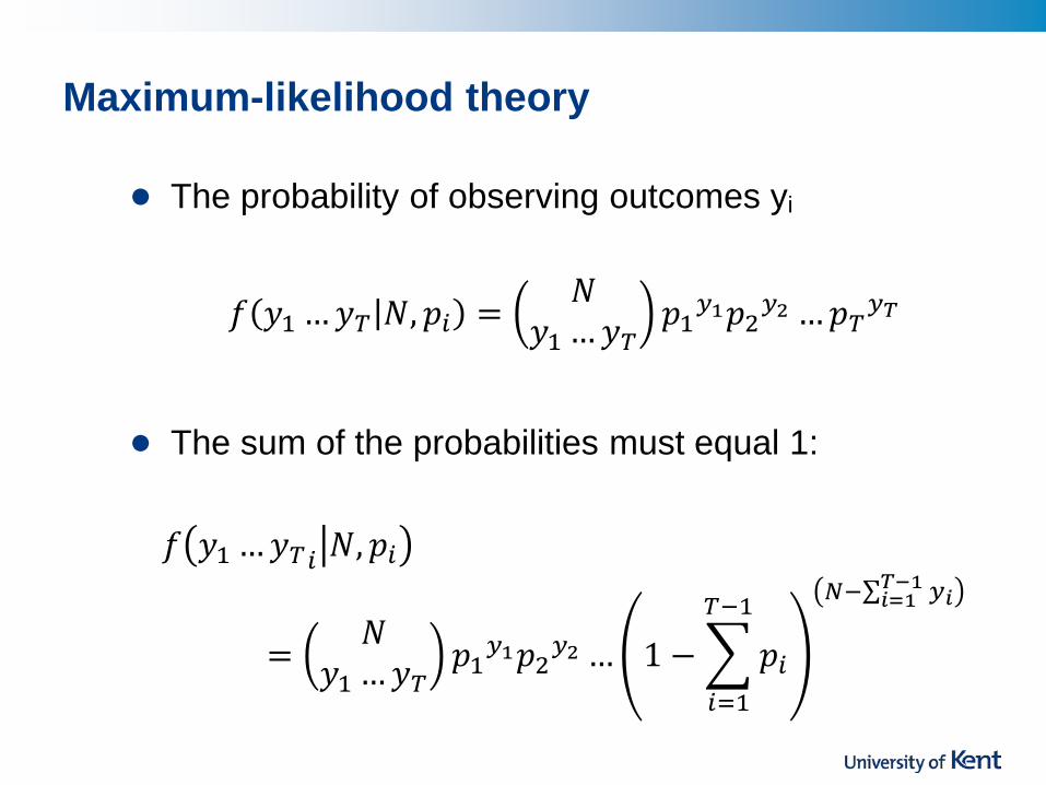
• The probability of observing outcomes yi
𝑓 𝑦1 …𝑦𝑇 𝑁,𝑝𝑖 = 𝑁𝑦1 …𝑦𝑇
𝑝1𝑦1𝑝2𝑦2 …𝑝𝑇𝑦𝑇
Maximum-likelihood theory
• The probability of observing outcomes yi
𝑓 𝑦1 …𝑦𝑇 𝑁,𝑝𝑖 = 𝑁𝑦1 …𝑦𝑇
𝑝1𝑦1𝑝2𝑦2 …𝑝𝑇𝑦𝑇
• The sum of the probabilities must equal 1: 𝑓 𝑦1 …𝑦𝑇𝑖 𝑁,𝑝𝑖
= 𝑁𝑦1 …𝑦𝑇
𝑝1𝑦1𝑝2𝑦2 … 1 −�𝑝𝑖
𝑇−1
𝑖=1
𝑁−∑ 𝑦𝑖𝑇−1𝑖=1
Maximum-likelihood theory
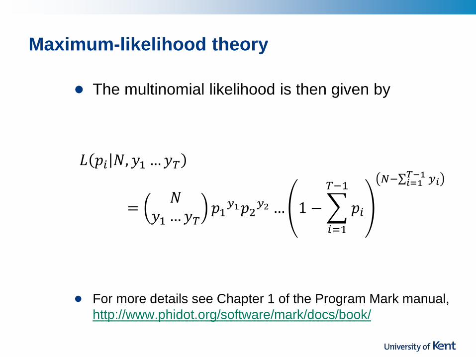
• The multinomial likelihood is then given by
𝐿 𝑝𝑖 𝑁,𝑦1 …𝑦𝑇
= 𝑁𝑦1 …𝑦𝑇
𝑝1𝑦1𝑝2𝑦2 … 1 −�𝑝𝑖
𝑇−1
𝑖=1
𝑁−∑ 𝑦𝑖𝑇−1𝑖=1
• For more details see Chapter 1 of the Program Mark manual, http://www.phidot.org/software/mark/docs/book/
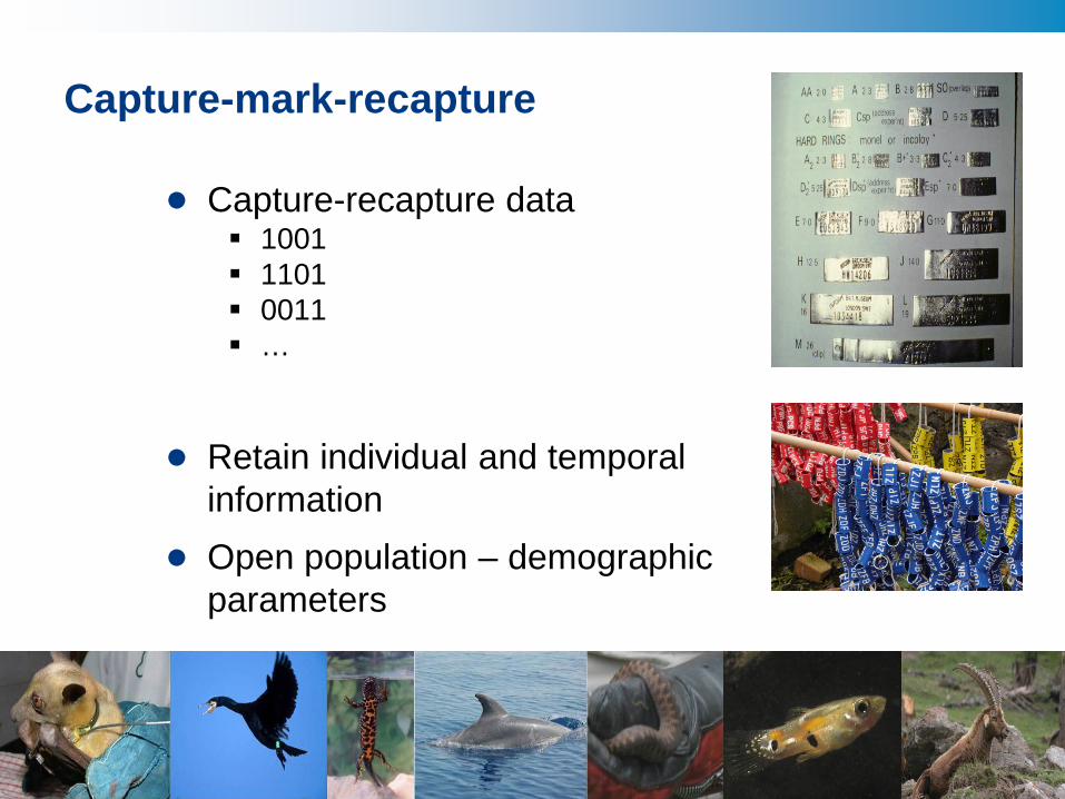
Capture-mark-recapture
• Capture-recapture data 1001 1101 0011 …
• Retain individual and temporal information
• Open population – demographic parameters
Cormack-Jolly-Seber model
• Population is open – births and death can occur within the study period
• Population size is no longer the parameter of interest
• φ: survival probability
• Condition on first capture
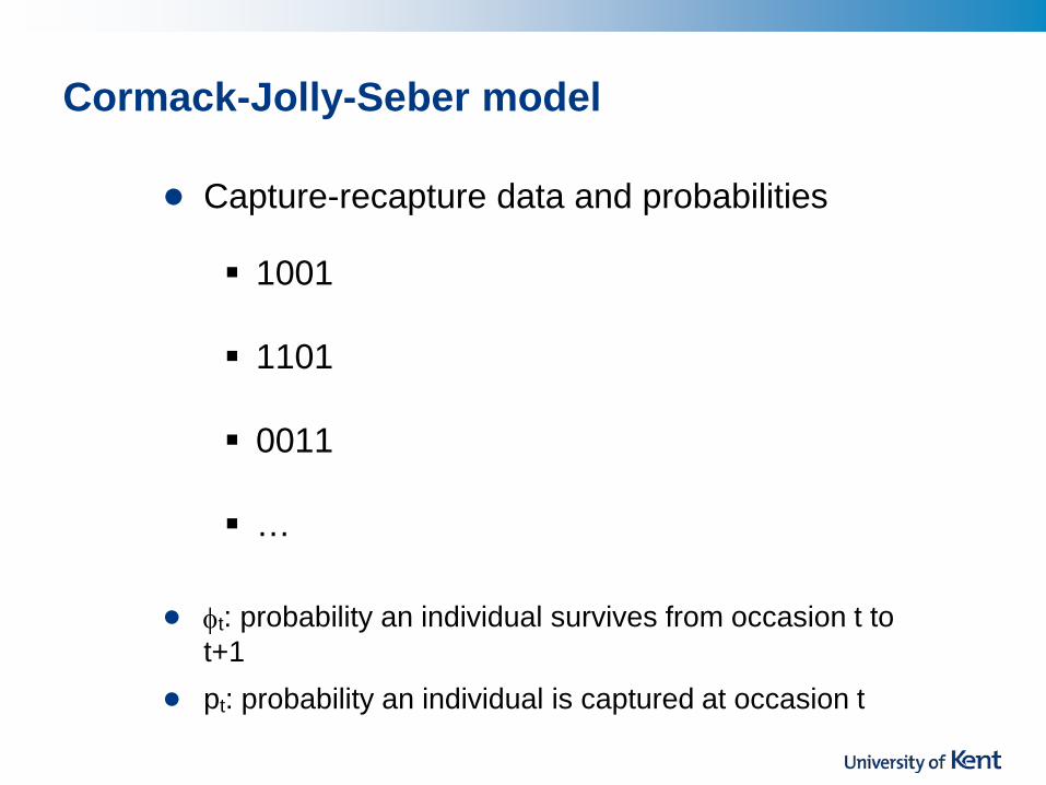
Cormack-Jolly-Seber model
• Capture-recapture data and probabilities
1001
1101 0011
…
• φt: probability an individual survives from occasion t to
t+1
• pt: probability an individual is captured at occasion t
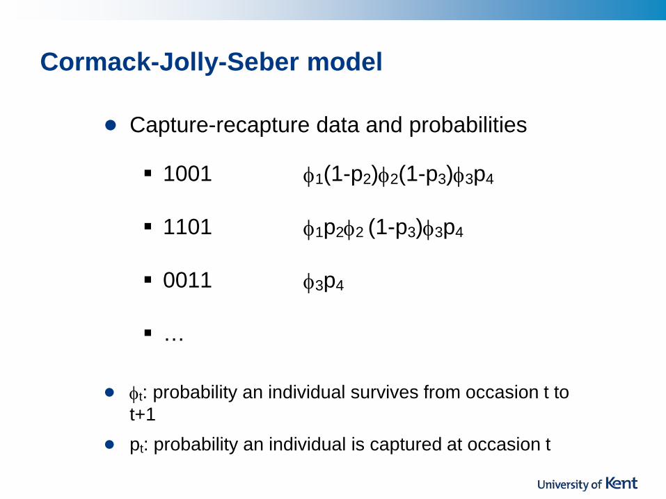
Cormack-Jolly-Seber model
• Capture-recapture data and probabilities
1001 φ1(1-p2)φ2(1-p3)φ3p4
1101 φ1p2φ2 (1-p3)φ3p4 0011 φ3p4
…
• φt: probability an individual survives from occasion t to
t+1
• pt: probability an individual is captured at occasion t
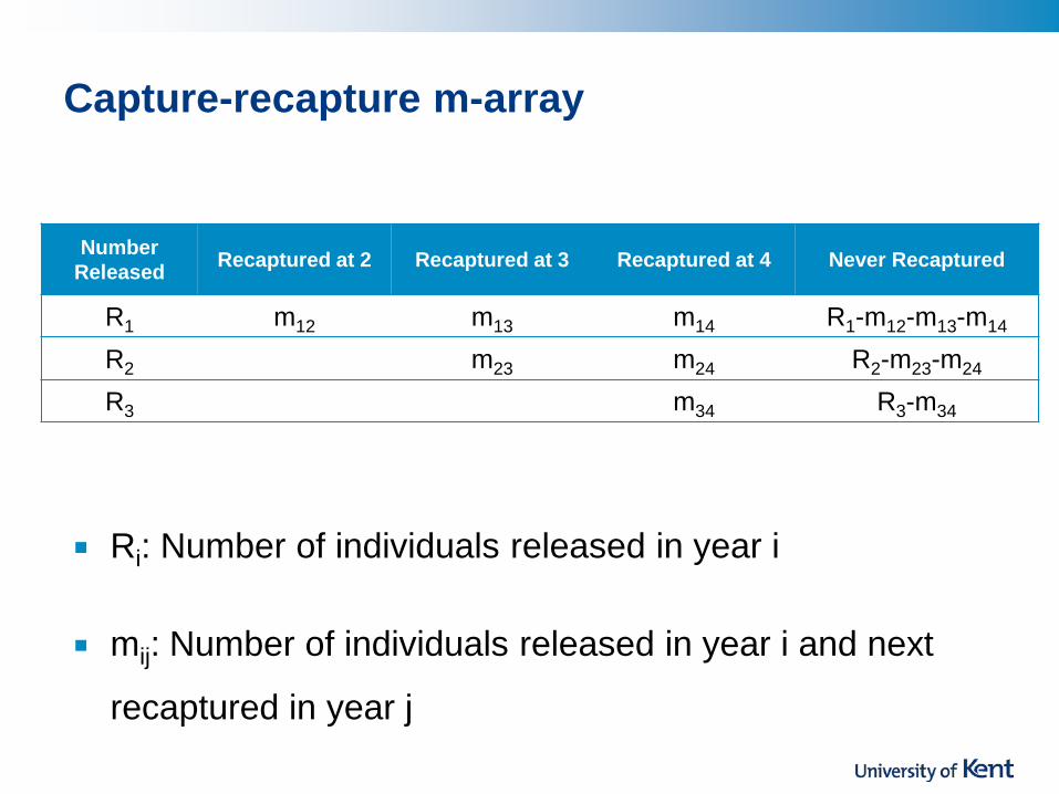
Capture-recapture m-array
Number Released Recaptured at 2 Recaptured at 3 Recaptured at 4 Never Recaptured
R1 m12 m13 m14 R1-m12-m13-m14
R2 m23 m24 R2-m23-m24
R3 m34 R3-m34
Ri: Number of individuals released in year i
mij: Number of individuals released in year i and next
recaptured in year j
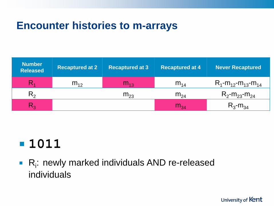
Encounter histories to m-arrays
1011 Ri: newly marked individuals AND re-released
individuals
Number Released Recaptured at 2 Recaptured at 3 Recaptured at 4 Never Recaptured
R1 m12 m13 m14 R1-m12-m13-m14
R2 m23 m24 R2-m23-m24
R3 m34 R3-m34
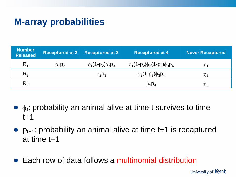
M-array probabilities
• φt: probability an animal alive at time t survives to time t+1
• pt+1: probability an animal alive at time t+1 is recaptured at time t+1
• Each row of data follows a multinomial distribution
Number Released Recaptured at 2 Recaptured at 3 Recaptured at 4 Never Recaptured
R1 φ1p2 φ1(1-p2)φ2p3 φ1(1-p2)φ2(1-p3)φ3p4 χ1
R2 φ2p3 φ2(1-p3)φ3p4 χ2
R3 φ3p4 χ3
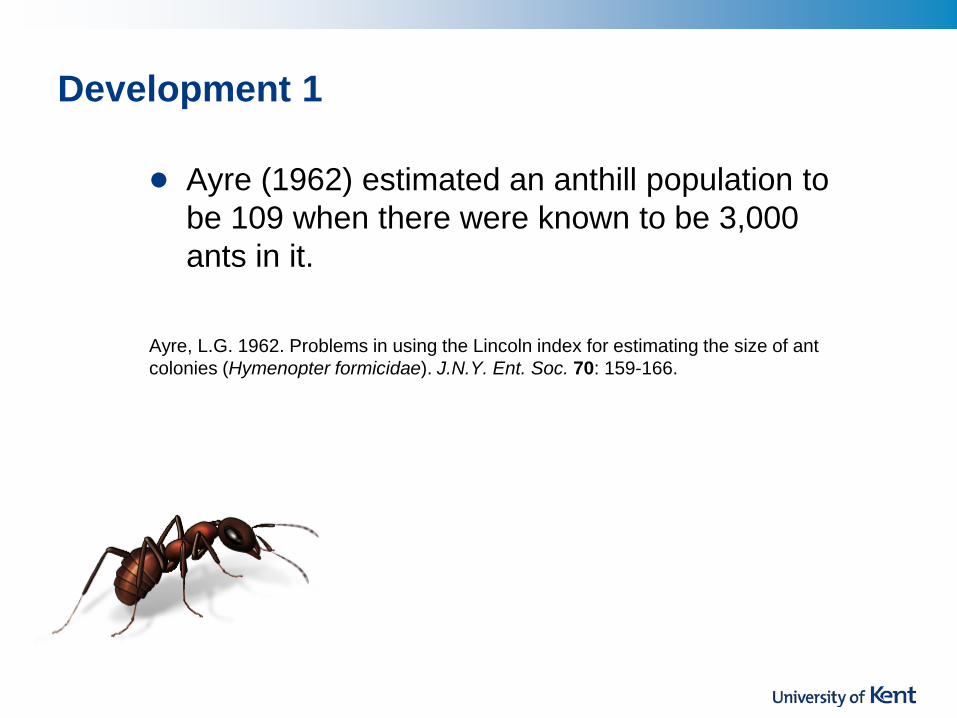
Development 1
• Ayre (1962) estimated an anthill population to be 109 when there were known to be 3,000 ants in it.
Ayre, L.G. 1962. Problems in using the Lincoln index for estimating the size of ant colonies (Hymenopter formicidae). J.N.Y. Ent. Soc. 70: 159-166.
Lincoln-Petersen Estimate: Model Assumptions
• Population is closed
• Marks are permanent and do not affect catchability
• All animals equally likely to be captured in each sample
• Sampling time is short in relation to total time
• Samples are taken randomly
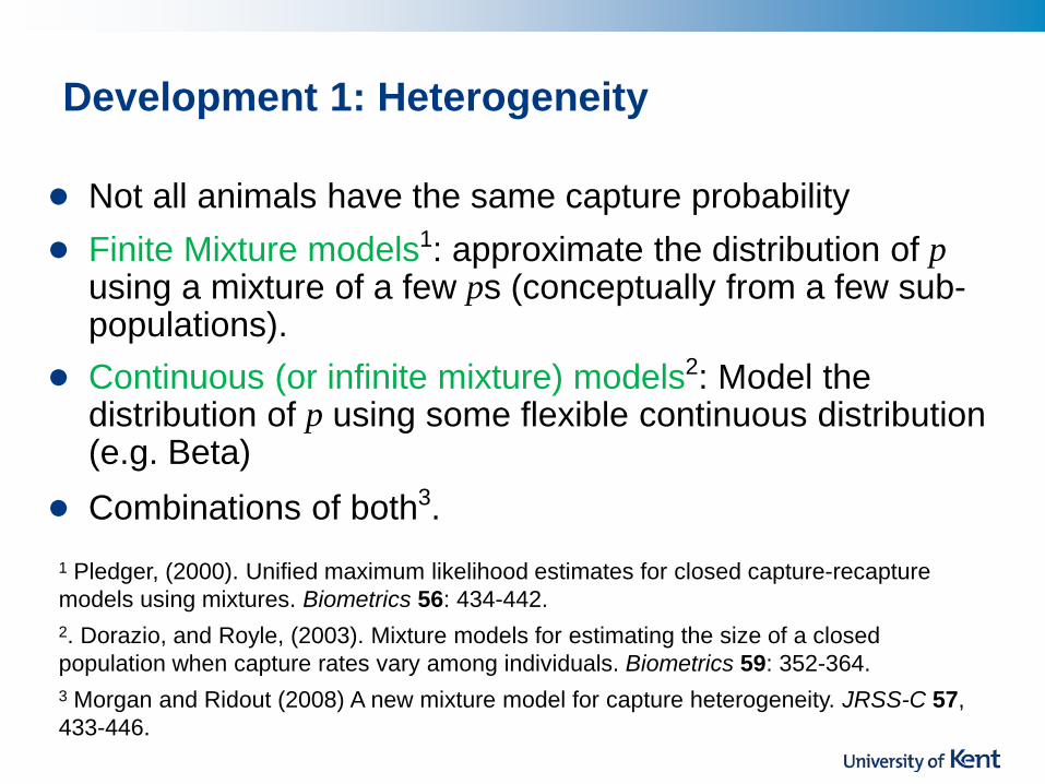
Development 1: Heterogeneity
• Not all animals have the same capture probability
• Finite Mixture models1: approximate the distribution of p using a mixture of a few ps (conceptually from a few sub-populations).
• Continuous (or infinite mixture) models2: Model the distribution of p using some flexible continuous distribution (e.g. Beta)
• Combinations of both3. 1 Pledger, (2000). Unified maximum likelihood estimates for closed capture-recapture models using mixtures. Biometrics 56: 434-442. 2. Dorazio, and Royle, (2003). Mixture models for estimating the size of a closed population when capture rates vary among individuals. Biometrics 59: 352-364. 3 Morgan and Ridout (2008) A new mixture model for capture heterogeneity. JRSS-C 57, 433-446.
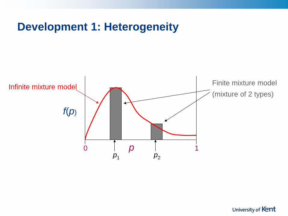
f(p)
p 1 0
Finite mixture model (mixture of 2 types)
p1 p2
Infinite mixture model
Development 1: Heterogeneity

Development 2: Modelling movement
Site A
Site B
Site C
),( CAψ
),( ACψ
),( BCψ
),( ABψ
),( CBψ
),( BAψ
),( BBψ),( CCψ
),( AAψ
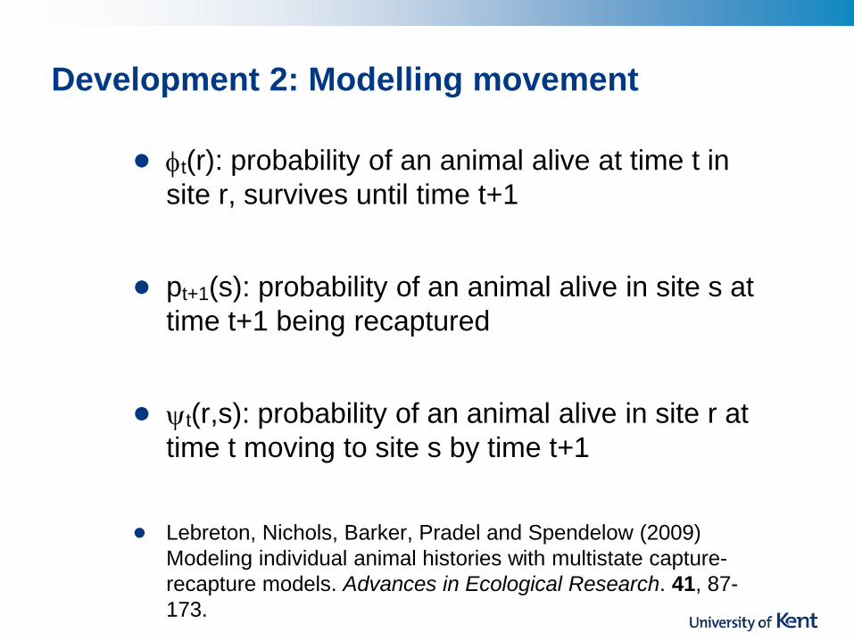
Development 2: Modelling movement
• φt(r): probability of an animal alive at time t in site r, survives until time t+1
• pt+1(s): probability of an animal alive in site s at time t+1 being recaptured
• ψt(r,s): probability of an animal alive in site r at time t moving to site s by time t+1
• Lebreton, Nichols, Barker, Pradel and Spendelow (2009) Modeling individual animal histories with multistate capture-recapture models. Advances in Ecological Research. 41, 87-173.
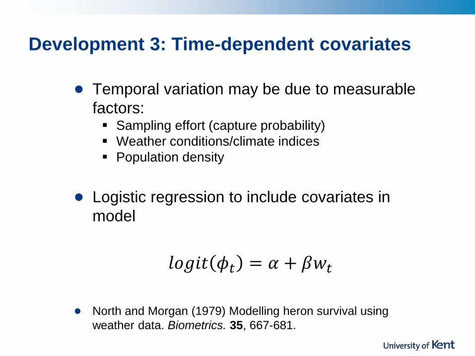
Development 3: Time-dependent covariates
• Temporal variation may be due to measurable factors: Sampling effort (capture probability) Weather conditions/climate indices Population density
• Logistic regression to include covariates in model
𝑙𝑙𝑙𝑙𝑙 𝜙𝑡 = 𝛼 + 𝛽𝑤𝑡 • North and Morgan (1979) Modelling heron survival using
weather data. Biometrics. 35, 667-681.
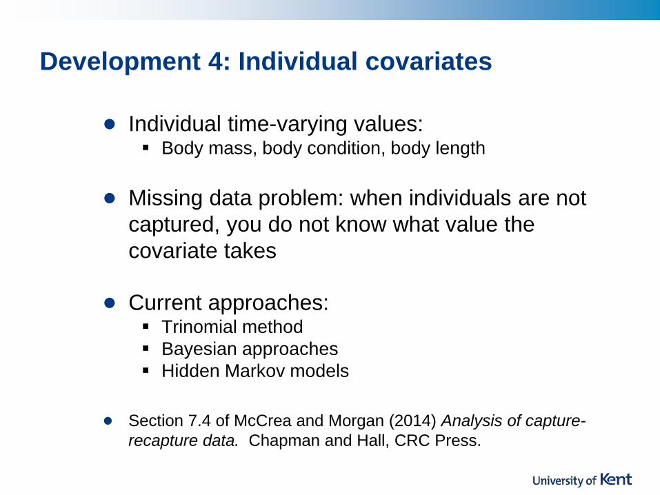
Development 4: Individual covariates
• Individual time-varying values: Body mass, body condition, body length
• Missing data problem: when individuals are not captured, you do not know what value the covariate takes
• Current approaches: Trinomial method Bayesian approaches Hidden Markov models
• Section 7.4 of McCrea and Morgan (2014) Analysis of capture-recapture data. Chapman and Hall, CRC Press.
Useful References
• Williams, Nichols and Conroy (2002) Analysis and management of animal populations. Academic Press.
• Lebreton, Burnham and Clobert (1992) Modeling survival and testing biological hypotheses using marked animals: a unified approach with case studies. Ecological monographs. 62, 67-118.
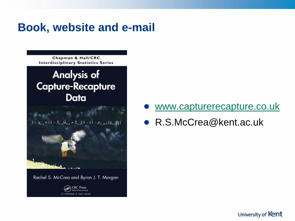
Book, website and e-mail
• www.capturerecapture.co.uk