Introduction to Black Hole Informatics

Introduction to Black Hole Informatics- Lecture 3 -

Lárus Thorlacius

2018 Arnold Sommerfeld School on “Black Holes and Quantum Information”

Arnold Sommerfeld Center for Theoretical Physics Munich, 8 - 12 October 2018

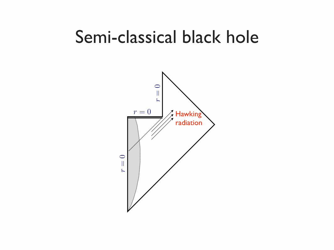
Semi-classical black hole

r=

0

r = 0r

=0

Hawkingradiation

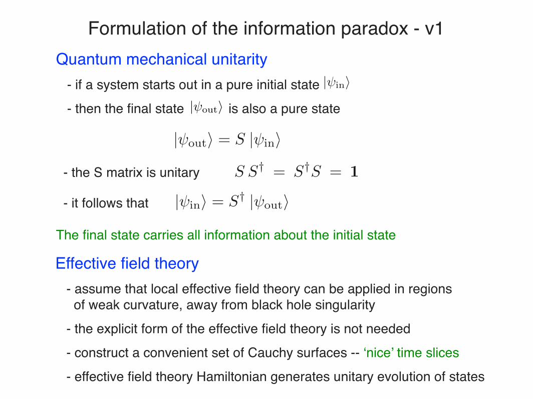
Formulation of the information paradox - v1Quantum mechanical unitarity

- if a system starts out in a pure initial state

- then the final state is also a pure state

- the S matrix is unitary

- it follows that

The final state carries all information about the initial state

|�in�

|�out�

|�out� = S |�in�

|�in� = S† |�out�

S S† = S†S = 1

Effective field theory

- assume that local effective field theory can be applied in regions of weak curvature, away from black hole singularity

- the explicit form of the effective field theory is not needed

- construct a convenient set of Cauchy surfaces -- ‘nice’ time slices

- effective field theory Hamiltonian generates unitary evolution of states

�out

�ext

�bh P�in

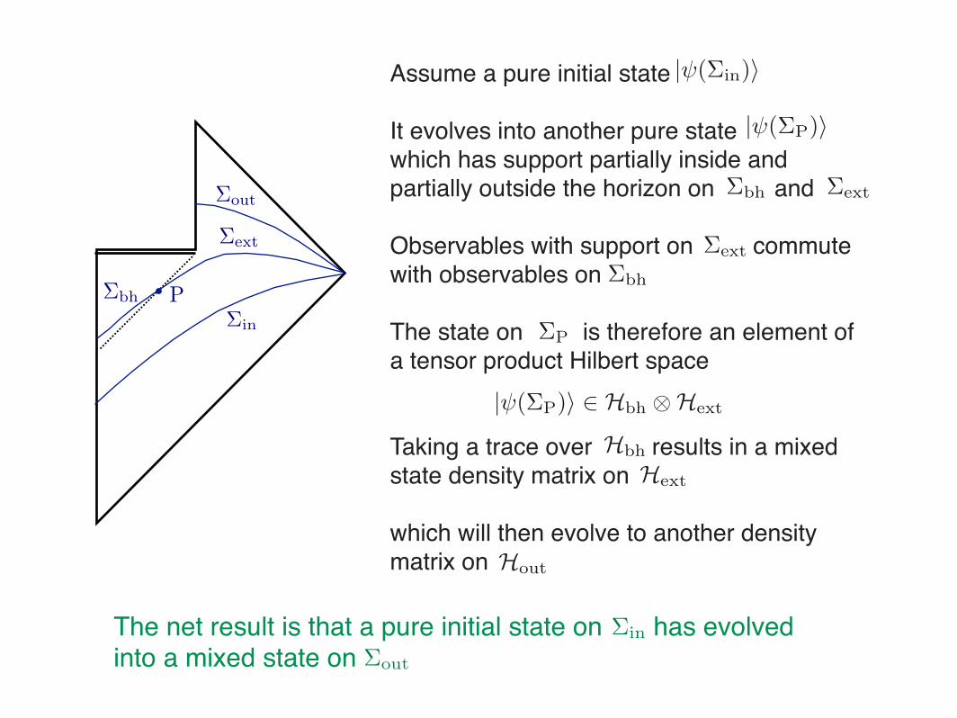
Assume a pure initial state

It evolves into another pure statewhich has support partially inside and partially outside the horizon on and

Observables with support on commutewith observables on

The state on is therefore an element ofa tensor product Hilbert space

Taking a trace over results in a mixed state density matrix on

which will then evolve to another density matrix on

|�(�in)�

|�(�P)�

|�(�P)⌅ ⇥ Hbh �Hext

�bh �ext

�P

Hbh

Hext

Hout

�ext

�bh

The net result is that a pure initial state on has evolvedinto a mixed state on

�in

�out

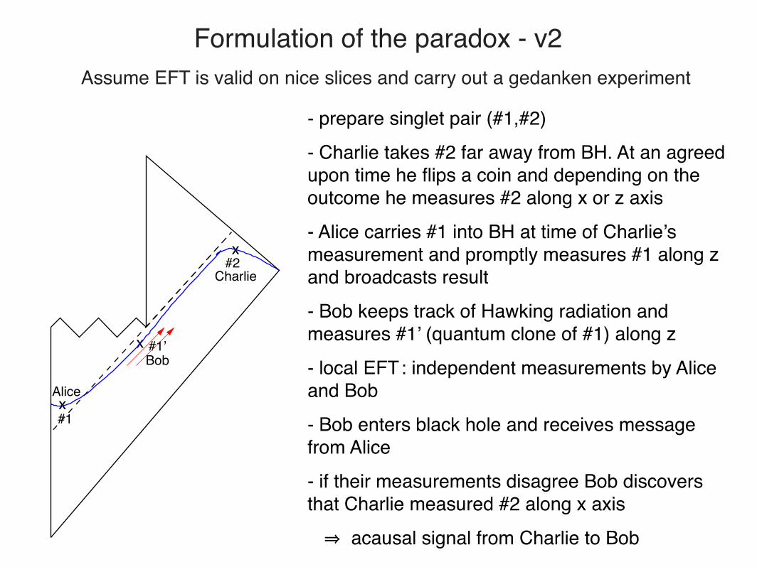
Formulation of the paradox - v2

- prepare singlet pair (#1,#2)

- Charlie takes #2 far away from BH. At an agreed upon time he flips a coin and depending on the outcome he measures #2 along x or z axis

- Alice carries #1 into BH at time of Charlie’s measurement and promptly measures #1 along z and broadcasts result

- Bob keeps track of Hawking radiation and measures #1’ (quantum clone of #1) along z

- local EFT : independent measurements by Alice and Bob

- Bob enters black hole and receives message from Alice

- if their measurements disagree Bob discovers that Charlie measured #2 along x axis

⇒ acausal signal from Charlie to Bob

Assume EFT is valid on nice slices and carry out a gedanken experiment

x

x

x #1’

#2

#1

Charlie

Alice

Bob

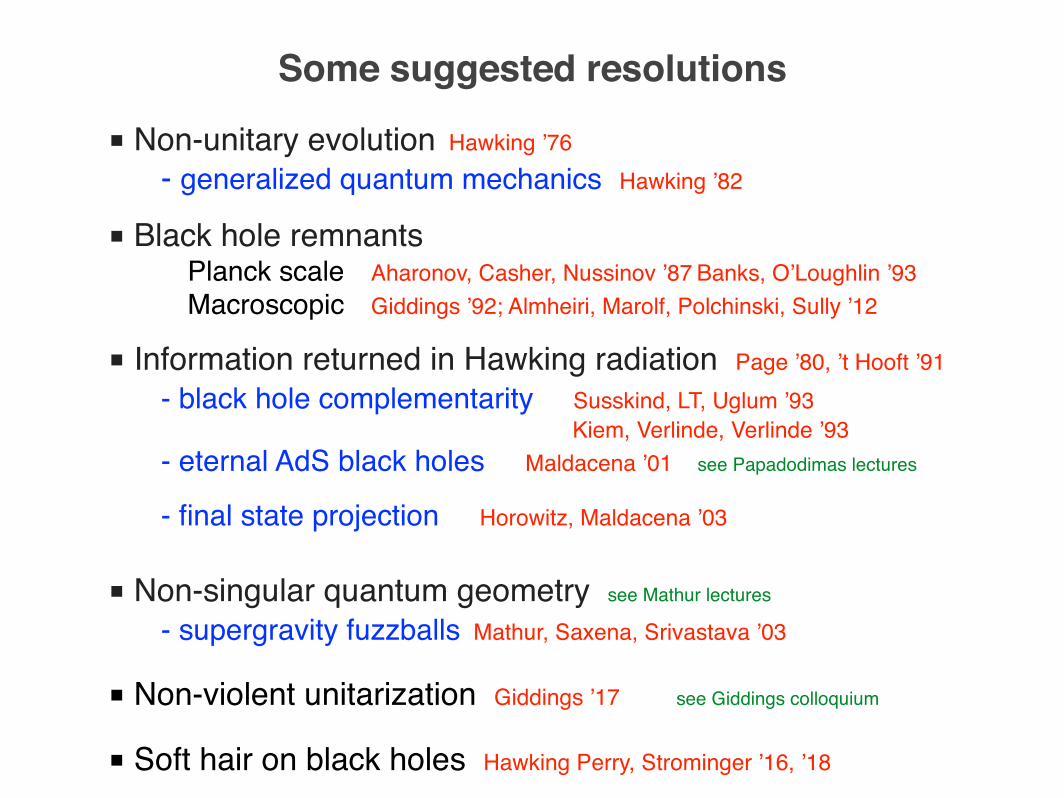
Some suggested resolutions

■ Non-unitary evolution Hawking ’76

- generalized quantum mechanics Hawking ’82

■ Black hole remnants

Planck scale Aharonov, Casher, Nussinov ’87 Banks, O’Loughlin ’93 Macroscopic Giddings ’92; Almheiri, Marolf, Polchinski, Sully ’12

■ Information returned in Hawking radiation Page ’80, ’t Hooft ’91

- black hole complementarity Susskind, LT, Uglum ’93 Kiem, Verlinde, Verlinde ’93 - eternal AdS black holes Maldacena ’01 see Papadodimas lectures

- final state projection Horowitz, Maldacena ’03

■ Non-singular quantum geometry see Mathur lectures

- supergravity fuzzballs Mathur, Saxena, Srivastava ’03

■ Non-violent unitarization Giddings ’17 see Giddings colloquium ■ Soft hair on black holes Hawking Perry, Strominger ’16, ’18

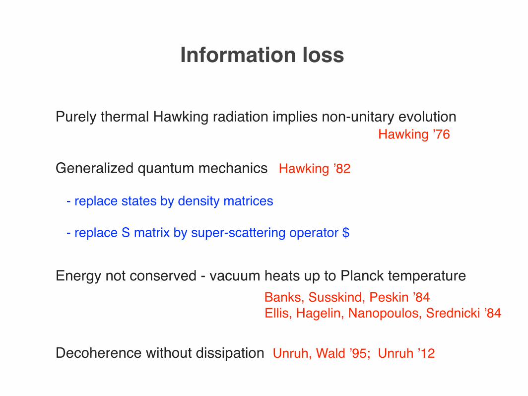
Information loss

Purely thermal Hawking radiation implies non-unitary evolution Hawking ’76

Generalized quantum mechanics Hawking ’82 - replace states by density matrices

- replace S matrix by super-scattering operator $

Energy not conserved - vacuum heats up to Planck temperature

Banks, Susskind, Peskin ’84 Ellis, Hagelin, Nanopoulos, Srednicki ’84

Decoherence without dissipation Unruh, Wald ’95; Unruh ’12

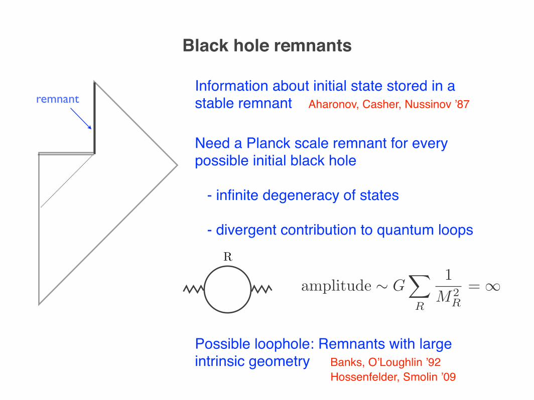
Black hole remnants

R

amplitude � G�

R

1M2

R

=⇥

remnantInformation about initial state stored in a stable remnant Aharonov, Casher, Nussinov ’87

Need a Planck scale remnant for every possible initial black hole

- infinite degeneracy of states

- divergent contribution to quantum loops

Possible loophole: Remnants with large intrinsic geometry Banks, O’Loughlin ’92 Hossenfelder, Smolin ’09

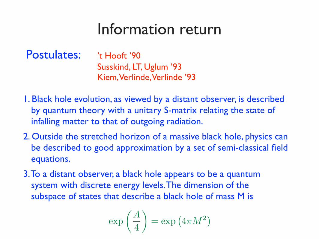
Information return

Postulates: ’t Hooft ’90 Susskind, LT, Uglum ’93 Kiem, Verlinde, Verlinde ’93

1. Black hole evolution, as viewed by a distant observer, is described by quantum theory with a unitary S-matrix relating the state of infalling matter to that of outgoing radiation.

2. Outside the stretched horizon of a massive black hole, physics can be described to good approximation by a set of semi-classical field equations.

3. To a distant observer, a black hole appears to be a quantum system with discrete energy levels. The dimension of the subspace of states that describe a black hole of mass M is

exp⇤

A

4

⌅= exp

�4�M2

⇥

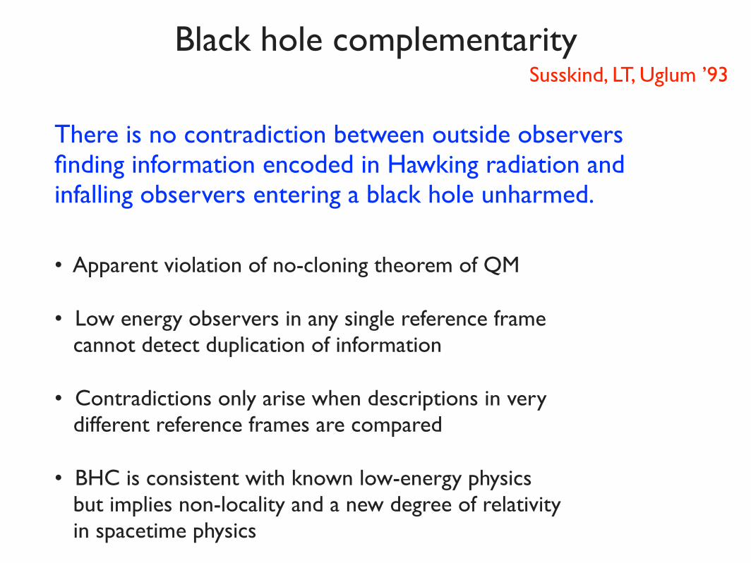
Black hole complementaritySusskind, LT, Uglum ’93

There is no contradiction between outside observers finding information encoded in Hawking radiation and infalling observers entering a black hole unharmed.

• Apparent violation of no-cloning theorem of QM

• Low energy observers in any single reference frame cannot detect duplication of information

• Contradictions only arise when descriptions in very different reference frames are compared

• BHC is consistent with known low-energy physics but implies non-locality and a new degree of relativity in spacetime physics

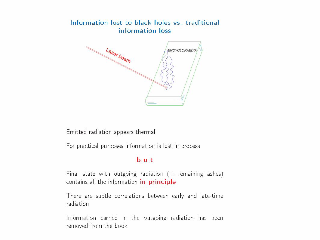
Laser beam

ENCYCLOPAEDIA

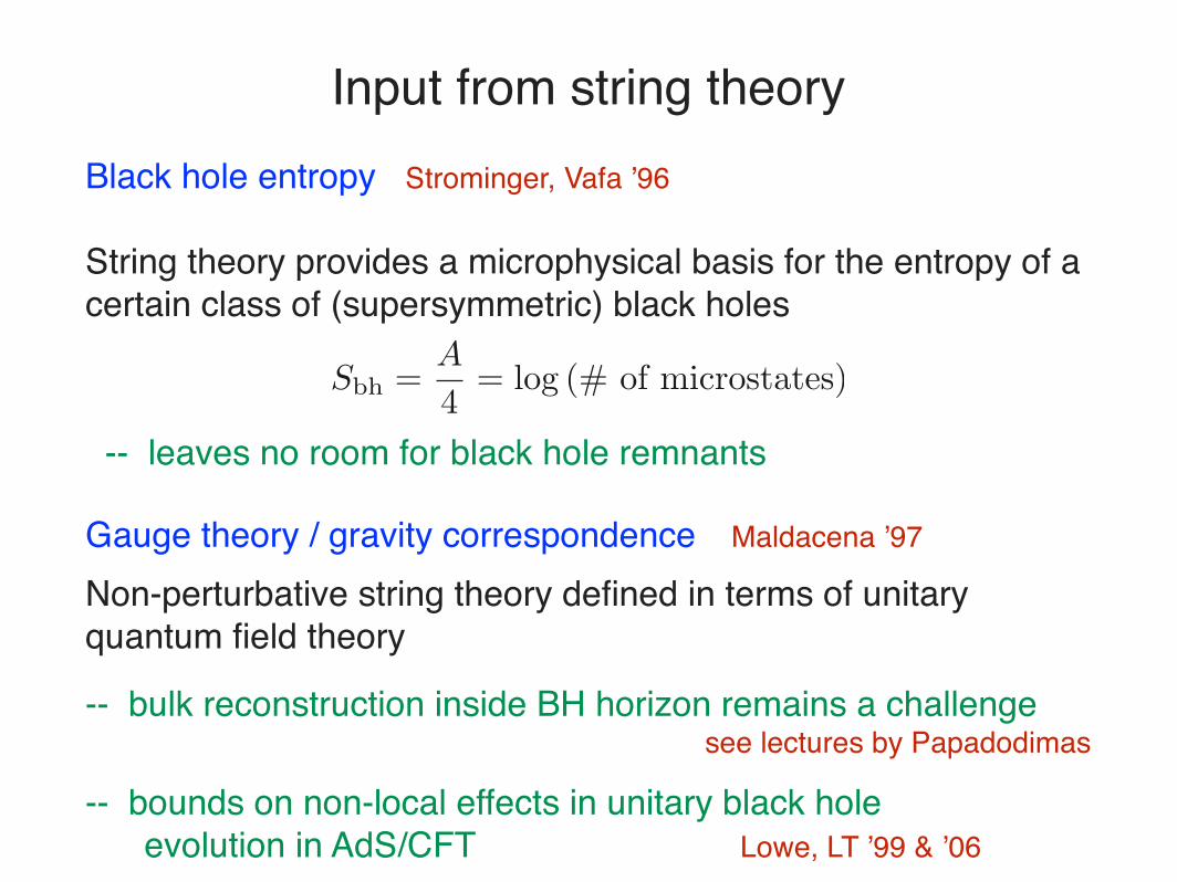
Input from string theoryBlack hole entropy Strominger, Vafa ’96

String theory provides a microphysical basis for the entropy of a certain class of (supersymmetric) black holes

-- leaves no room for black hole remnants

Sbh =A

4= log (# of microstates)

Gauge theory / gravity correspondence Maldacena ’97

Non-perturbative string theory defined in terms of unitary quantum field theory

-- bulk reconstruction inside BH horizon remains a challengesee lectures by Papadodimas

-- bounds on non-local effects in unitary black hole evolution in AdS/CFT Lowe, LT ’99 & ’06

Tests of black hole complementarity

Membrane paradigm Thorne, Price, MacDonald ’82-’86

Replace black hole by a stretched horizon -- a membrane ‘near’ the event horizon

In astrophysical applications ‘near’ means close compared to f.ex. distance to companion in a binary system

Quantum mechanical stretched horizon Susskind, LT, Uglum’93

Minimal stretching:

Unspecified microphysics with

Ash = Aeh + 1

# of states = exp(A/4)

Gedanken experiments Susskind, LT ’93

Apparent violations of BHC can be traced to assumptions about physics at Planck energy (or higher)

Information paradox involves Planck scale in subtle ways

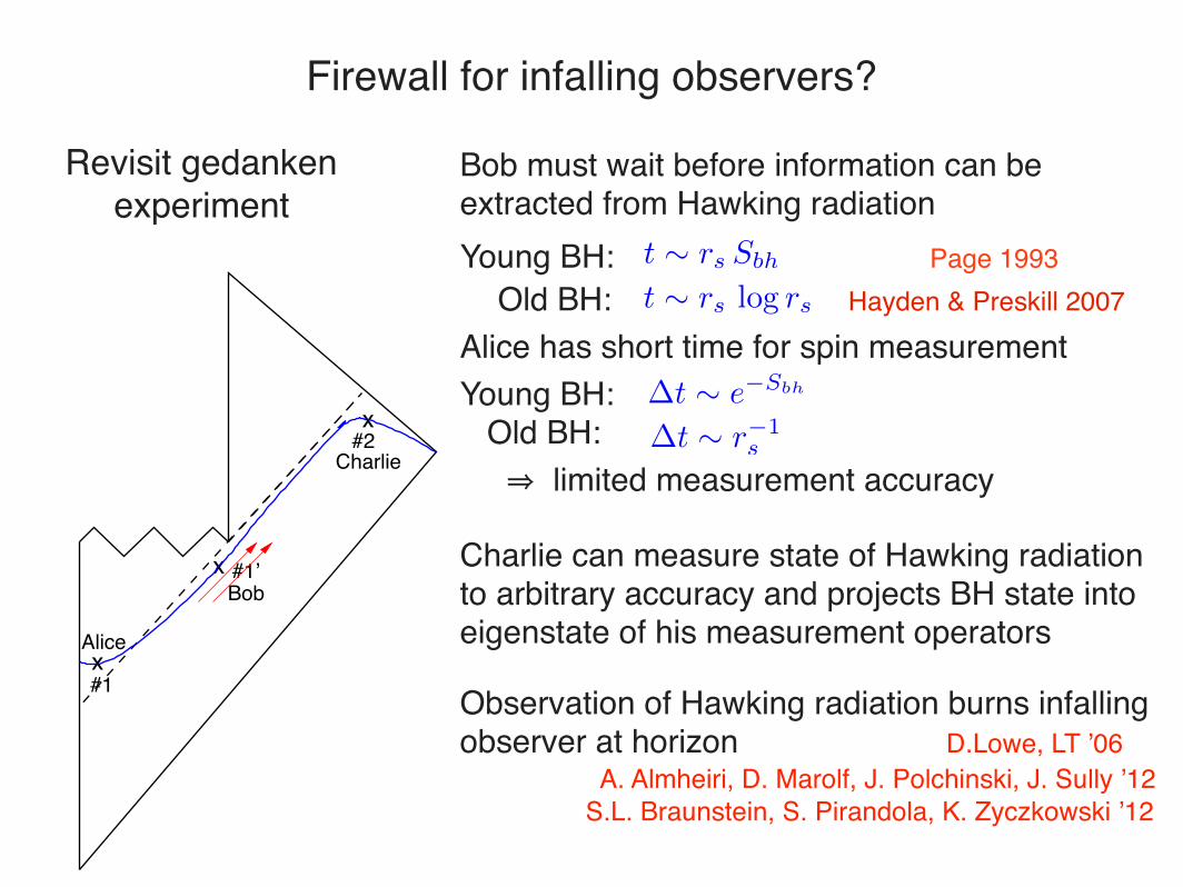
Firewall for infalling observers?

Revisit gedanken experiment

Bob must wait before information can beextracted from Hawking radiationYoung BH: Page 1993 Old BH: Hayden & Preskill 2007Alice has short time for spin measurementYoung BH: Old BH: ⇒ limited measurement accuracy

Charlie can measure state of Hawking radiation to arbitrary accuracy and projects BH state into eigenstate of his measurement operators

Observation of Hawking radiation burns infalling observer at horizon D.Lowe, LT ’06 A. Almheiri, D. Marolf, J. Polchinski, J. Sully ’12 S.L. Braunstein, S. Pirandola, K. Zyczkowski ’12

t ⇠ rs Sbh

t ⇠ rs log rs

�t ⇠ e�Sbh

�t ⇠ r�1s

x

x

x #1’

#2

#1

Charlie

Alice

Bob

A holographic view of the black hole interior

D. Lowe & L.T. - JHEP 1801 (2018) 049 JHEP 1612 (2016) 024 JHEP 1512 (2015) 096 Phys. Lett. B 737 (2014) 320

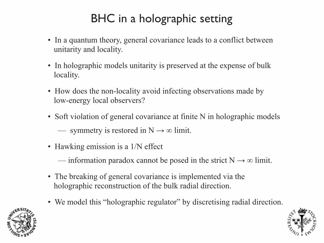
• In a quantum theory, general covariance leads to a conflict between unitarity and locality.

• In holographic models unitarity is preserved at the expense of bulk locality.

• How does the non-locality avoid infecting observations made by low-energy local observers?

• Soft violation of general covariance at finite N in holographic models

— symmetry is restored in N → ∞ limit.

• Hawking emission is a 1/N effect

— information paradox cannot be posed in the strict N → ∞ limit.

• The breaking of general covariance is implemented via the holographic reconstruction of the bulk radial direction.

• We model this “holographic regulator” by discretising radial direction.

BHC in a holographic setting

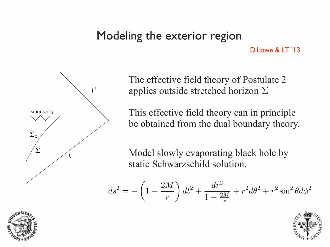
D.Lowe & LT ’13

Model slowly evaporating black hole by static Schwarzschild solution.

S

S0

singularity

i+

i-

Figure 1: Penrose diagram for black hole evaporation. Σ0 is the global horizon and Σ is a stretched

horizon.

The stretched horizon is a surface outside the global black hole horizon that remains

timelike. Outside observers ascribe non-trivial microphysical dynamics to the stretched

horizon that serves to absorb, thermalize, and eventually re-emit the information contained

in infalling matter. The usual thermodynamics of black holes is assumed to arise from a

coarse graining of this (unspecified) microscopic dynamics. From the point of view of outside

observers, no information ever enters the black hole in this description and the stretched

horizon is the end of the road for all infalling matter. In that sense it is indeed a firewall.

According to the fourth postulate the story is very different for an infalling observer. The

spacetime curvature is weak at the horizon of a large black hole and an infalling observer

should not notice anything out of the ordinary upon crossing the horizon. In a recent paper

Almheiri et al. [3] claim, however, that the first two postulates imply that an infalling

observer must also see a firewall. In other words, that the fourth postulate is inconsistent

with the others.

The microscopic stretched horizon in [1] was placed at a proper distance of order the

Planck length away from the global horizon. More generally in the present work, we require

3

The effective field theory of Postulate 2 applies outside stretched horizon ⌃

II. NON-ROTATING BLACK HOLE EVAPORATION IN 3+1 DIMENSIONS:

PROBLEMS AND SOLUTIONS

A. Mode expansions and vacua

In this section we consider a massless conformally coupled scalar field. Issues of

back-reaction will be ignored, and re-examined in the following section. The metric in

Schwarzschild coordinates takes the form

ds

2= �

✓1� 2M

r

◆dt

2+

dr

2

1� 2Mr

+ r

2d✓

2+ r

2sin

2✓d�

2.

In these coordinates, a complete set of modes in the exterior region may be obtained by

separating the equation of motion, and defining the tortoise radial coordinate

r⇤ = r + 2M log

⇣r

2M

� 1

⌘.

The angular and time dependence may be handled straightforwardly, and the radial equation

can be mapped into a scattering problem with a step-like potential separating the behavior at

r ! 1 from the region r ! 2M [9]. This leads to a natural decomposition into independent

modes that we refer to as in-going and out-going [23]:

u

in

(x) = (4⇡!)

�1/2e

�i!t

R

in

l

(!; r)Y

lm

(✓,�)

u

out

(x) = (4⇡!)

�1/2e

�i!t

R

out

l

(!; r)Y

lm

(✓,�) (1)

with

R

out

l

(!; r) ⇠

8><

>:

r

�1e

i!r⇤+ A

out

l

(!)r

�1e

�i!r⇤, r ! 2M

B

l

(!)r

�1e

i!r⇤, r ! 1

R

in

l

(!; r) ⇠

8><

>:

B

l

(!)r

�1e

�i!r⇤, r ! 2M

r

�1e

�i!r⇤+ A

in

l

(!)r

�1e

i!r⇤, r ! 1 .

Scattering off the gravitational field leads to “grey body” factors, so a mode that is purely

outgoing near infinity contains an ingoing component near the horizon, and likewise a mode

that is purely ingoing near the horizon contains an outgoing component near infinity.

The Unruh vacuum is defined by requiring the modes incoming at past null infinity to

be purely positive frequency with respect to t, and while those outgoing from the past

4

Modeling the exterior region

This effective field theory can in principle be obtained from the dual boundary theory.

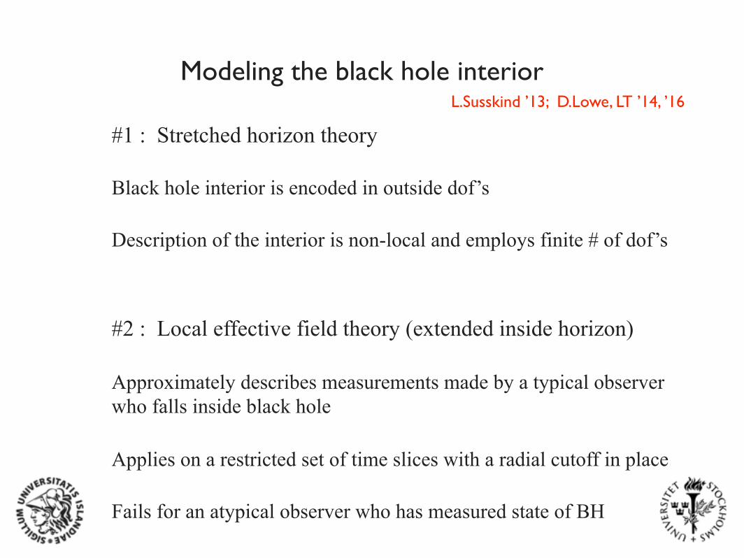
#2 : Local effective field theory (extended inside horizon)

Approximately describes measurements made by a typical observer who falls inside black hole

Applies on a restricted set of time slices with a radial cutoff in place

Black hole interior is encoded in outside dof’s

Description of the interior is non-local and employs finite # of dof’s

#1 : Stretched horizon theory

Fails for an atypical observer who has measured state of BH

L.Susskind ’13; D.Lowe, LT ’14, ’16

Modeling the black hole interior

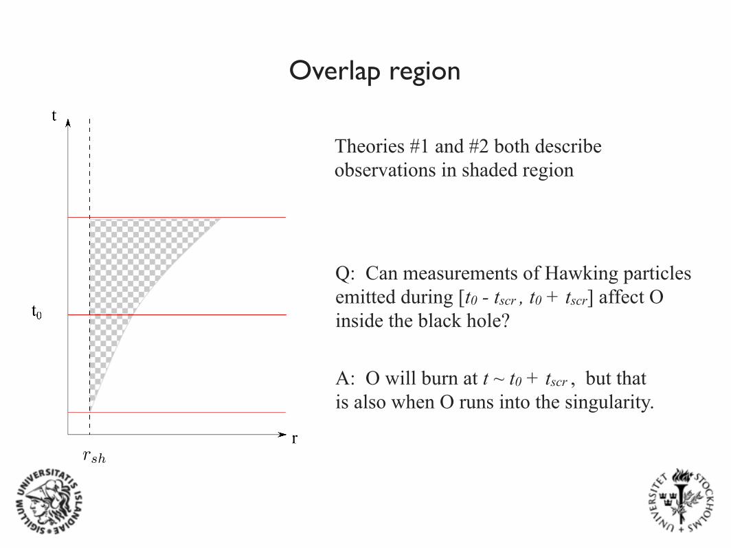
Q: Can measurements of Hawking particles emitted during [t0 - tscr , t0 + tscr] affect O inside the black hole?

Theories #1 and #2 both describe observations in shaded region

A: O will burn at t ~ t0 + tscr , but that is also when O runs into the singularity.

Overlap region

t

r

t0

t0+tscr

rsh

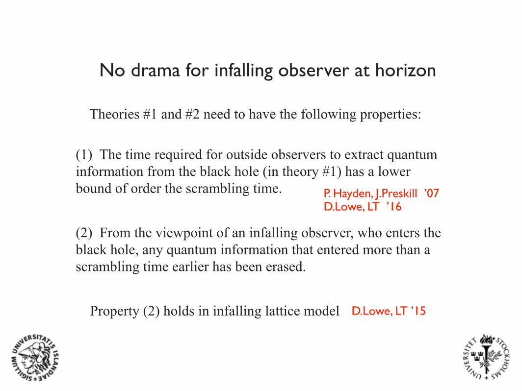
Theories #1 and #2 need to have the following properties:

No drama for infalling observer at horizon

D.Lowe, LT ’15Property (2) holds in infalling lattice model

(2) From the viewpoint of an infalling observer, who enters the black hole, any quantum information that entered more than a scrambling time earlier has been erased.

(1) The time required for outside observers to extract quantum information from the black hole (in theory #1) has a lower bound of order the scrambling time. P. Hayden, J.Preskill ’07

D.Lowe, LT ’16

Breakdown of bulk description

We want to model a laboratory that falls into a black hole.

Early on the lab is well described by the bulk effective Hamiltonian of theory #2.

The lab has a complementary description in terms of theory #1 and must eventually decohere with respect to the exact Hamiltonian.

This will appear highly non-local from the viewpoint of theory #2.

In a toy model we find that the decoherence time matches the scrambling time, which is also when lab approaches the singularity.

Results support the idea that singularity approach is complementary to decoherence of the infalling state.

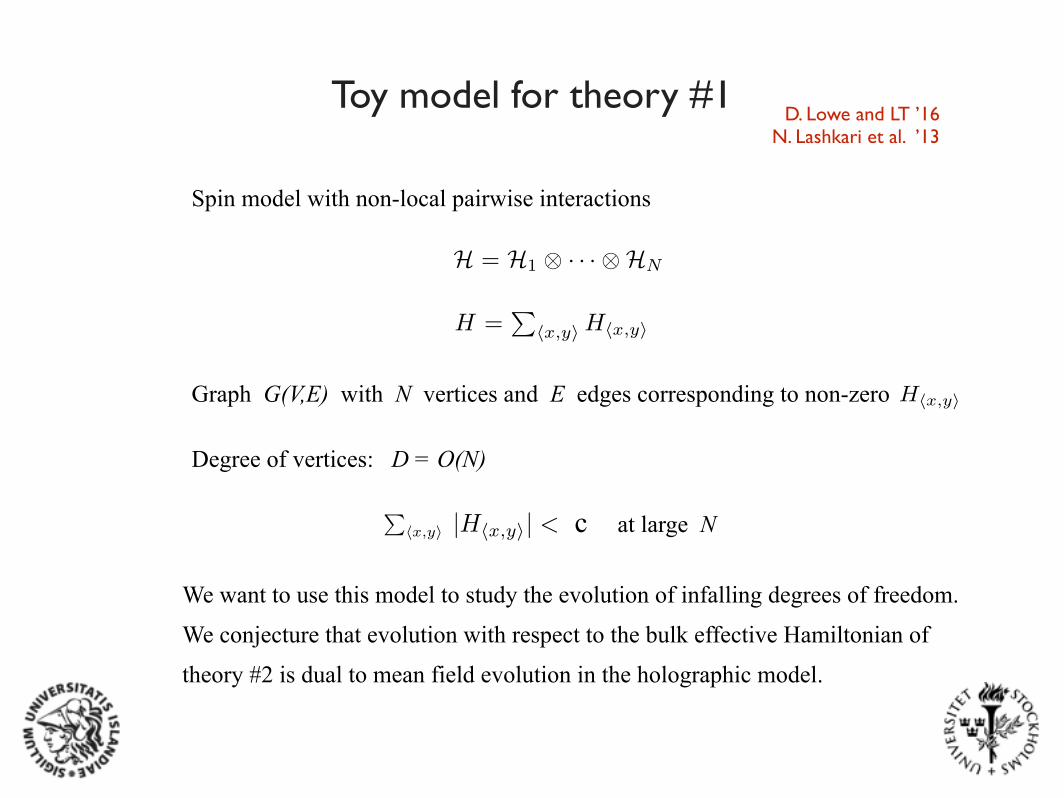
Toy model for theory #1

We want to use this model to study the evolution of infalling degrees of freedom.

We conjecture that evolution with respect to the bulk effective Hamiltonian of

theory #2 is dual to mean field evolution in the holographic model.

D. Lowe and LT ’16 N. Lashkari et al. ’13

for some choice of � < 1. We are not aware of prior appearances of this definition of decoherence timein the literature. This definition should be useful in many other contexts.

In the following we will mostly be interested in studying finite dimensional spin systems. In thisclass of models, we can reformulate the condition (2.3) as a condition on the trace distance using theresults of [11]. We recall the definition

k S � �Sk1 = TrS

q( S � �S)

†( S � �S) (2.4)

In [11] it is shown that|S( S)� S(�S)| k S � �Sk1 log n (2.5)

for two different density matrices in HS . Therefore the definition of the decoherence time can bereformulated as

k S(td)� �S(td)k1 = � (2.6)

for some fixed constant � < 1 and some suitable choice for �S . The state �S(t) should be chosen tomaintain purity under time evolution for the subsystem of interest, but minimize the trace distanceas a function of time so the bound (2.5) is as useful as possible. For the models considered here, wewill choose �S to evolve according to a local mean field Hamiltonian, as we describe below.

In [12] the statement of fast scrambling was defined in a similar way. The key distinction isthat scrambling involves a global mixing of the system, rather than only the mixing of a particularsubsystem of interest. The condition for scrambling would then require that, (2.6) should hold for allsubsystems, suitably defined, rather than some single small subsystem, as typically considered in thedecoherence problem.

3 Toy Holographic Model

While it is interesting to try to derive an effective holographic model for the horizon degrees of freedomof a black hole from some more fundamental description such as AdS/CFT or the Matrix Model, ourstrategy will be to make some minimal assumptions about such a description, and hope that it carriesover to a more precise reconstruction. The key assumption we will make of the model is that it exhibitsfast scrambling in the sense of [13], with a scrambling time

t ⇠ � logSBH

with � the inverse Hawking temperature of a black hole hole with energy E and SBH the Bekenstein-Hawking entropy of the black hole. Later we will also be interested in carrying out computations inthe model for highly entangled states that will model the state of an old black hole entangled with itsHawking radiation. As such, we assume the model contains enough degrees of freedom to model theinterior of the black hole and its immediate vicinity. Thus we make the identification that S ⇠ N thenumber of sites in the model, and � will be scaled out of the problem. The near-horizon region willnot contain all the symmetries of the asymptotic region, so we do not expect conformal symmetry (asin AdS/CFT) or supersymmetry (as in the BFSS model) to be crucial in formulating this effectivemodel. At best the holographic model should contain a version of rotation/translation symmetry, andtime translation invariance.

A toy model that exhibits these features is discussed in [12]. This is a spin model with a non-local pairwise interaction. There are N distinct sites with the Hilbert space of tensor product formH = H1 ⌦ · · · ⌦HN . The sites interact via a pairwise Hamiltonian H =

Phx,yi Hhx,yi summing over

– 4 –




q( S � �S)

†( S � �S) (2.4)



k S(td)� �S(td)k1 = � (2.6)





t ⇠ � logSBH




– 4 –

Spin model with non-local pairwise interactions

Graph G(V,E) with N vertices and E edges corresponding to non-zero unordered pairs of sites. The Hamiltonian may therefore be associated with a graph G = (V,E) withN vertices V , and edges E corresponding to the non-zero Hhx,yi. In order to have fast scrambling, thedegree of the vertices D should be of order the size of the system. We shall then set D = N � 1. Tohave a sensible limit for large N , we take the pairwise interactions to be bounded |Hhx,yi| < c/D, forsome constant c.

The Lieb-Robinson result [14] places bounds on the norm of the commutator of operators localizedat different sites, as a function of time. For local interactions, this is to be interpreted as a proof offinite group velocity in nonrelativistic spin systems. In the case at hand, where interactions are non-local, the same method still yields a bound on the norm of the commutator for operators. In particular,in [12] it is shown that

k[OA(t), OB ]k 4

DkOAk kOBk |A|e8ct (3.1)

Here OX is a bounded norm operator acting in the Hilbert subspace of the sites in the set X, and Bis chosen to be a single site.

The condition for scrambling is set up in [12] as follows. Consider some Hilbert subspace H1

with dimension of order 1, maximally entangled with some reference system P, which experiences nointeractions. Here we set the system S = H1. Under time evolution, the entanglement between H1

and P will decay, which may be quantified by the trace distance

k PS(t⇤)� P(0)⌦ S(t⇤)k1 < ✏ rank P(0) (3.2)

for some constant ✏ ⌧ 1. This may in principle then be used as a definition of scrambling time. Abound on the time t⇤ can then be obtained by noting that it is bounded by the signaling time fromthe space S to its complement Sc, which may be bounded using (3.1).

First apply this to an initial state where S is a single site, and the complement subspace Sc hasdimension of order N . We assume the initial state is of product form | (0)i = | 1iNH1 ⌦ | 2iH2 ⌦· · ·⌦ | N iHN

. Applying (3.1) with B = S and A = Sc one finds the timescale t⇤ is of order a constant.For the black hole problem, the natural initial state to choose is instead one where the black hole

degrees of freedom are maximally entangled with the exterior Hawking radiation. Now essentially theroles of S and Sc are reversed. One takes the system S to be of size of order N , with some smallsubsystem in a factor pure state. The complement is then of size of order 1. To satisfy the bound (3.2)one again requires signaling between S and Sc, and this timescale is bounded by the Lieb-Robinsonresult. This yields a timescale of order logN as expected for a fast scrambling system.

4 Mean field and bulk evolution

At first sight, the results of the previous section are not encouraging for the black hole complementarityscenario. While one can build holographic models that exhibit fast scrambling with t⇤ proportionalto logN , it seems the decoherence time for some small Hilbert subspace in such models will be veryshort. This is, however, not the right question to ask in the black hole problem. Instead, what oneshould do is build a model for a laboratory that one sends into the black hole, and then ask whetherthat laboratory will have a decoherence time sufficiently long that they will not be able to distinguishquantum mechanics failing from their classical demise due to singularity approach.

The eventual failure of quantum mechanics in the infalling laboratory can be traced to the ex-istence of two distinct time evolutions for the state in the lab subspace. One of these will be theexact Hamiltonian evolution according to the holographic Hamiltonian H. The other will be definedaccording to a mean field Hamiltonian HMF , that we describe in more detail shortly, and corresponds

– 5 –

Degree of vertices: D = O(N)unordered pairs of sites. The Hamiltonian may therefore be associated with a graph G = (V,E) withN vertices V , and edges E corresponding to the non-zero Hhx,yi. In order to have fast scrambling, thedegree of the vertices D should be of order the size of the system. We shall then set D = N � 1. Tohave a sensible limit for large N , we take the pairwise interactions to be bounded |Hhx,yi| < c/D, forsome constant c.

The Lieb-Robinson result [14] places bounds on the norm of the commutator of operators localizedat different sites, as a function of time. For local interactions, this is to be interpreted as a proof offinite group velocity in nonrelativistic spin systems. In the case at hand, where interactions are non-local, the same method still yields a bound on the norm of the commutator for operators. In particular,in [12] it is shown that

k[OA(t), OB ]k 4

DkOAk kOBk |A|e8ct (3.1)

Here OX is a bounded norm operator acting in the Hilbert subspace of the sites in the set X, and Bis chosen to be a single site.

The condition for scrambling is set up in [12] as follows. Consider some Hilbert subspace H1

with dimension of order 1, maximally entangled with some reference system P, which experiences nointeractions. Here we set the system S = H1. Under time evolution, the entanglement between H1

and P will decay, which may be quantified by the trace distance

k PS(t⇤)� P(0)⌦ S(t⇤)k1 < ✏ rank P(0) (3.2)

for some constant ✏ ⌧ 1. This may in principle then be used as a definition of scrambling time. Abound on the time t⇤ can then be obtained by noting that it is bounded by the signaling time fromthe space S to its complement Sc, which may be bounded using (3.1).

First apply this to an initial state where S is a single site, and the complement subspace Sc hasdimension of order N . We assume the initial state is of product form | (0)i = | 1iNH1 ⌦ | 2iH2 ⌦· · ·⌦ | N iHN

. Applying (3.1) with B = S and A = Sc one finds the timescale t⇤ is of order a constant.For the black hole problem, the natural initial state to choose is instead one where the black hole

degrees of freedom are maximally entangled with the exterior Hawking radiation. Now essentially theroles of S and Sc are reversed. One takes the system S to be of size of order N , with some smallsubsystem in a factor pure state. The complement is then of size of order 1. To satisfy the bound (3.2)one again requires signaling between S and Sc, and this timescale is bounded by the Lieb-Robinsonresult. This yields a timescale of order logN as expected for a fast scrambling system.

4 Mean field and bulk evolution

At first sight, the results of the previous section are not encouraging for the black hole complementarityscenario. While one can build holographic models that exhibit fast scrambling with t⇤ proportionalto logN , it seems the decoherence time for some small Hilbert subspace in such models will be veryshort. This is, however, not the right question to ask in the black hole problem. Instead, what oneshould do is build a model for a laboratory that one sends into the black hole, and then ask whetherthat laboratory will have a decoherence time sufficiently long that they will not be able to distinguishquantum mechanics failing from their classical demise due to singularity approach.

The eventual failure of quantum mechanics in the infalling laboratory can be traced to the ex-istence of two distinct time evolutions for the state in the lab subspace. One of these will be theexact Hamiltonian evolution according to the holographic Hamiltonian H. The other will be definedaccording to a mean field Hamiltonian HMF , that we describe in more detail shortly, and corresponds

– 5 –




q( S � �S)

†( S � �S) (2.4)



k S(td)� �S(td)k1 = � (2.6)





t ⇠ � logSBH




– 4 –

c at large N

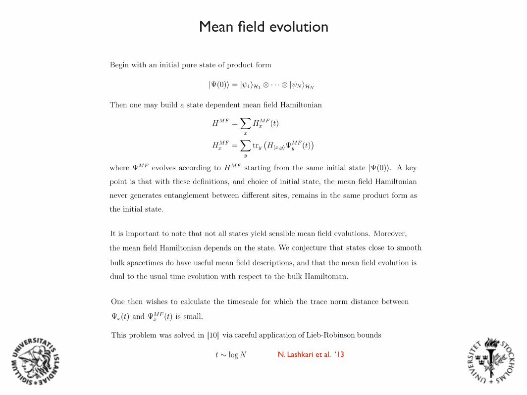
Mean field evolution

mechanics failing from their classical demise due to singularity approach.

If one uses the decoherence time defined according to (7), then one is appealing to the

subsystem N that the laboratory does not have access to. It is then not necessarily a

contraction then that the decoherence time defined this way does not scale with system size.

However if we use the definition in (5), the timescale is defined in terms of observables in

the lab subsystem. In the present section, we study this possibility.

To make sense of this we need two distinct time evolutions for the state in the lab

subspace. One of these will be the exact Hamiltonian evolution according to H. The other

will be defined according to a mean field Hamiltonian HMF that we describe in more detail

shortly.

It is important to note that not all states yield sensible mean field evolutions. Moreover,

as will be clear, the mean field Hamiltonian depends on the state. State dependence of the

holographic construction was emphasized in ... We conjecture that states close to smooth

bulk spacetimes do have useful mean field descriptions, and that the mean field evolution is

dual to the usual time evolution with respect to the bulk Hamiltonian.

The mean field approximation to the time evolution of a density matrix is considered in

some generality in [12]. Begin with an initial pure state of product form

| (0)i = | 1iH1 ⌦ · · ·⌦ | NiHN (8)

Then one may build a state dependent mean field Hamiltonian

HMF=

X

x

HMFx (t)

HMFx =

X

y

try

�Hhx,yi MF

y (t)�

where MF evolves according to HMF starting from the same initial state | (0)i. A key

point is that with these definitions, and choice of initial state, the mean field Hamiltonian

never generates entanglement between different sites, remains in the same product form as

the initial state.

One then wishes to calculate the timescale for which the trace norm distance between

x(t) and MFx (t) is small. This problem was solved in [10] for the spin model considered

above, via careful application of Lieb-Robinson bounds applied to an expansion of the matrix

element⌦ (0)| � MF

x (t)| (0)↵ = 1� ⌦

MFx (t)| x(t)| MF

x (t)↵

(9)

7










shortly.








| (0)i = | 1iH1 ⌦ · · ·⌦ | NiHN (8)


HMF=

X

x

HMFx (t)

HMFx =

X

y

try

�Hhx,yi MF

y (t)�




the initial state.





x (t)| (0)↵ = 1� ⌦

MFx (t)| x(t)| MF

x (t)↵

(9)

7










shortly.








| (0)i = | 1iH1 ⌦ · · ·⌦ | NiHN (8)


HMF=

X

x

HMFx (t)

HMFx =

X

y

try

�Hhx,yi MF

y (t)�




the initial state.





x (t)| (0)↵ = 1� ⌦

MFx (t)| x(t)| MF

x (t)↵

(9)

7










shortly.








| (0)i = | 1iH1 ⌦ · · ·⌦ | NiHN (8)


HMF=

X

x

HMFx (t)

HMFx =

X

y

try

�Hhx,yi MF

y (t)�




the initial state.





x (t)| (0)↵ = 1� ⌦

MFx (t)| x(t)| MF

x (t)↵

(9)

7










shortly.








| (0)i = | 1iH1 ⌦ · · ·⌦ | NiHN (8)


HMF=

X

x

HMFx (t)

HMFx =

X

y

try

�Hhx,yi MF

y (t)�




the initial state.





x (t)| (0)↵ = 1� ⌦

MFx (t)| x(t)| MF

x (t)↵

(9)

7










shortly.








| (0)i = | 1iH1 ⌦ · · ·⌦ | NiHN (8)


HMF=

X

x

HMFx (t)

HMFx =

X

y

try

�Hhx,yi MF

y (t)�




the initial state.





x (t)| (0)↵ = 1� ⌦

MFx (t)| x(t)| MF

x (t)↵

(9)

7










shortly.








| (0)i = | 1iH1 ⌦ · · ·⌦ | NiHN (8)


HMF=

X

x

HMFx (t)

HMFx =

X

y

try

�Hhx,yi MF

y (t)�




the initial state.





x (t)| (0)↵ = 1� ⌦

MFx (t)| x(t)| MF

x (t)↵

(9)

7










shortly.








| (0)i = | 1iH1 ⌦ · · ·⌦ | NiHN (8)


HMF=

X

x

HMFx (t)

HMFx =

X

y

try

�Hhx,yi MF

y (t)�




the initial state.





x (t)| (0)↵ = 1� ⌦

MFx (t)| x(t)| MF

x (t)↵

(9)

7










shortly.








| (0)i = | 1iH1 ⌦ · · ·⌦ | NiHN (8)


HMF=

X

x

HMFx (t)

HMFx =

X

y

try

�Hhx,yi MF

y (t)�




the initial state.





x (t)| (0)↵ = 1� ⌦

MFx (t)| x(t)| MF

x (t)↵

(9)

7










shortly.








| (0)i = | 1iH1 ⌦ · · ·⌦ | NiHN (8)


HMF=

X

x

HMFx (t)

HMFx =

X

y

try

�Hhx,yi MF

y (t)�




the initial state.





x (t)| (0)↵ = 1� ⌦

MFx (t)| x(t)| MF

x (t)↵

(9)

7










shortly.








| (0)i = | 1iH1 ⌦ · · ·⌦ | NiHN (8)


HMF=

X

x

HMFx (t)

HMFx =

X

y

try

�Hhx,yi MF

y (t)�




the initial state.





x (t)| (0)↵ = 1� ⌦

MFx (t)| x(t)| MF

x (t)↵

(9)

7

by making a Dyson series expansion in H � HMFx . This matrix element in turn places a

bound on the trace distance between the states (4). Using the result of [9], this in turn

places a bound on the von Neumann entropy H( x(t)). One finds

⌦

MFx (t)| x(t)| MF

x (t)↵ c0

Dec

00t (10)

where c0and c00 are constants independent of N . For D = N � 1 these quantities become of

order 1 when t ⇠ logN .

Making contact with black hole physics, the holographic description should be useful both

inside and outside the black hole horizon. An initial state of the form (8) is relevant outside

the black hole horizon, so is not immediately relevant for the physics of interior degrees of

freedom.

However suppose instead we choose an initial state where we have a pairwise entanglement

between H2k and H2k+1 for all k � 1. Then we can almost map the problem into the one

just considered by coarse graining, and viewing H2k ⌦ H2k+1 as a pure state on a single

coarse grained site. The new feature is that the coarse grained Hamiltonian now has a self-

interaction term. Such a term must be treated exactly in the mean field approximation. For

this initial state, we therefore define

HMF=

X

x

HMFx (t)

HMFx = Hhx,xi +

X

y\xtry

�Hhx,yi MF

y (t)�

where the sums are over coarse grained sites x = 1, · · · , N/2. This illustrates the state

dependence of the mean field approximation. With this Hamiltonian, we may then proceed

as above to compute the trace distance between the mean field state and the exact evolution,

or equivalently the von Neumann entropy of the exact reduced density matrix, obtaining

the same scaling with N (though different constants c0 and c00).

This is now a nice model for an old evaporating black hole, where the interior degrees

of freedom are maximally entangled with the exterior Hawking radiation. The decoher-

ence time, defined according to the definition (3) is now of order t ⇠ logN matching the

scrambling time.

8

N. Lashkari et al. ’13

Mean field evolution for infalling laboratory

JHEP01(2018)049

systems. The description is very crude however and to correctly describe the short-range

Newtonian gravity limit of freely falling laboratories in detail would require a much more

detailed specification of the holographic model, which for now we steer clear of.

In gauge/gravity duality in general, the map between the holographic model and the

gravitational spacetime is extremely nonlocal. In the present case, we are already led to

use a maximally nonlocal interaction between the spins to generate fast scrambling. We

may view the spins as living on a lattice on a spherical surface embedded in the black hole

spacetime. For example, we can consider approximately spherically symmetric states in

four-dimensional spacetime, in which case the lattice will span the θ,φ coordinates of a

Schwarzschild solution.

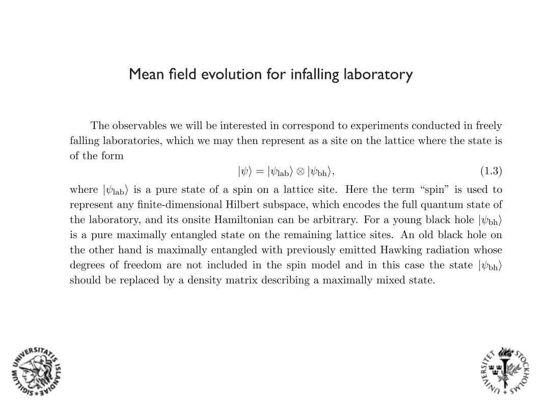
The observables we will be interested in correspond to experiments conducted in freely

falling laboratories, which we may then represent as a site on the lattice where the state is

of the form

|ψ⟩ = |ψlab⟩ ⊗ |ψbh⟩, (1.3)

where |ψlab⟩ is a pure state of a spin on a lattice site. Here the term “spin” is used to

represent any finite-dimensional Hilbert subspace, which encodes the full quantum state of

the laboratory, and its onsite Hamiltonian can be arbitrary. For a young black hole |ψbh⟩is a pure maximally entangled state on the remaining lattice sites. An old black hole on

the other hand is maximally entangled with previously emitted Hawking radiation whose

degrees of freedom are not included in the spin model and in this case the state |ψbh⟩should be replaced by a density matrix describing a maximally mixed state.

Scrambling is accomplished via the nonlocal coupling between different sites. Time

evolution with respect to the holographic Hamiltonian will evolve the state (1.3) forward

in time. The main problem in mapping holographic time evolution to bulk time evolution

involves correctly identifying the relevant bulk timeslices. In this regard, we follow [1] where

a rather generic freely falling Planck lattice was considered as a bulk regulator. In [2] we

found that many of the properties of holographic states are reproduced when matched

with such a bulk description. On the bulk gravity side this evolution corresponds to

propagating the laboratory inwards along a radial timelike geodesic. Since the holographic

Hamiltonian eventually evolves the state toward a stationary thermal state, we are able to

match the holographic time coordinate t with the bulk Killing vector time, and we assume

this matching can be carried out near the black hole a few Schwarzschild radii outside

the horizon.

If we form the reduced density matrix of the laboratory site, by tracing over the Hilbert

subspace associated with all other sites, the evolution will behave as an open quantum sys-

tem [8, 9]. In particular, the state |ψlab⟩ will not experience local unitary evolution due to

interactions with other sites. Ordinary local interactions with the surrounding spacetime

account for part of this effect, but the dominant effect comes down to the nonlocal inter-

action with distant sites. One of the main questions we are interested in is to quantify the

degree to which these nonlocal effects disrupt the experience of unitary quantum mechanics

for the falling laboratory.

To study this we formulate a mean field approximation for the evolution of the

state (1.3). Time dependent mean field approximations have previously been studied in

– 4 –

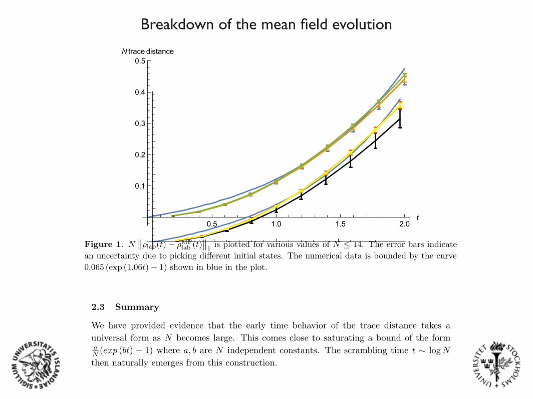
Breakdown of the mean field evolutionJHEP01(2018)049

0.5 1.0 1.5 2.0t

0.1

0.2

0.3

0.4

0.5N trace distance

Figure 1. N∥∥ρlab(t)− ρMF

lab (t)∥∥1is plotted for various values of N ≤ 14. The error bars indicate

an uncertainty due to picking different initial states. The numerical data is bounded by the curve0.065 (exp (1.06t)− 1) shown in blue in the plot.

where ρMF(0) = ρ(0). The early time behavior shows a time dependence that converges

as N increases to an N -indepedent form. Likewise the error bars associated with the

average over initial states are small. Finally the function is bounded by a function of the

form 0.065 (exp (1.06t)− 1), allowing us to extract the scrambling time t ∼ β logN as a

characteristic timescale.

On somewhat longer timescales than shown in figure 1 the purity Trρ2lab(t), which

starts at 1, approaches that of a maximally mixed state (or 1/2 for a 2-state system).

After this a Loschmidt echo develops, as shown in figure 2. If we identify the mixing

timescale with the minimum of the purity, this is well fit by a logarithmic function

tp = −1.70 + 4.26 logN as shown in figure 3, providing another way to see the scrambling

time emerge from the evolution.

2.2 Modeling an old black hole

As a check on the previous results it is interesting to instead begin with the black hole sector

in a maximally mixed density matrix. With the present computations, this is most easily

accomplished by purifying the state. One way to accomplish this is to begin with the initial

state (2.2) but set the Hamiltonian to vanish on sites indexed by i even, and unchanged

when i is odd. The even sites then undergo trivial time evolution, but remain maximally

entangled with the odd sites. Finally we may act with a random unitary transformation

on the Hilbert subspace of the odd sites to generate a typical entangled state.

The results for Ntot ≤ 14 (i.e. Nbh ≤ 7) are shown in figure 4. Up to numerical errors

the results are the same as in the previous subsection for the early time behavior. Again

this shows that N∥∥ρlab(t)− ρMF

lab (t)∥∥1approaches an N independent limit, that is bounded

by a function of the form 0.061 (exp (1.04t)− 1).

– 8 –

JHEP01(2018)049

0.5 1.0 1.5 2.0t

0.1

0.2

0.3

0.4

N trace distance

Figure 4. N∥∥ρlab(t)− ρMF

lab (t)∥∥1is plotted for maximally mixed black hole density matrices,

representing an old black hole. The behavior is very similar to figure 1.

2.3 Summary

We have provided evidence that the early time behavior of the trace distance takes a

universal form as N becomes large. This comes close to saturating a bound of the formaN (exp (bt) − 1) where a, b are N independent constants. The scrambling time t ∼ logN

then naturally emerges from this construction.

3 Mean field theory

We now wish to study observables in the class of states described in the previous section.

One approach would be to carry out explicit numerical calculations but, as we have seen

above, the rapid growth of Hilbert space dimensions and limited computer power restricts

this to relatively modest values of N . We instead adopt a strategy that allows explicit

analytic calculations that are valid for large N . The first step is to reformulate the states

of interest as unentangled pure states in a coarse grained spin model and then carry out a

standard thermodynamic analysis.

3.1 Maximally entangled states in spin models

A maximally entangled state is unitary equivalent to a product state of the form (2.2),

where for simplicity we imagine each site contains a spin 1/2 degree of freedom. As shown

in [2], we may start with a generic maximally entangled state and perform a unitary

transformation to get such a state. Such a unitary transformation does not necessarily

commute with the Hamiltonian.

Now if we coarse grain, combining the sites k and k+1 into a single site, and the state

on each pair into a pure state on the coarse-grained lattice, we are left with an unentangled

– 10 –

The information paradox highlights the incompatibility between general relativity (locality + equivalence principle) and quantum physics (unitarity).

Gauge theory - gravity correspondence implies unitary black hole evolution.

Black hole complementarity provides a "phenomenological" description, which preserves unitarity and the equivalence principle, but requires giving up locality.

Typical infalling observers do not see drama on their way towards a black hole formed from a generic pure state. (Special pure states, as well as special observers, exist for which this is not true.)

An approximate description of observers in the black hole interior can be given in terms of an effective field theory, defined on a limited set of time slices, such that no drama is seen until near the singularity.

A spin system with a nonlocal pairwise interaction provides a toy model for the holographic description of the black hole interior.

Evolution with respect to the bulk effective Hamiltonian is dual to mean field evolution in the holographic model.

Decoherence time for an infalling lab matches black hole scrambling time.

Summary

Observer in free fall near horizon: t = proper time, y = constant

Horizon is at y = t . Observer enters black hole at t = y = 0 .

Coordinate system for infalling observer

Lattice model: Discretise y coordinate

S.Corley & T.Jacobson ’97; D.Lowe, LT ’15

Infalling lattice model

pt

= �E = � �1� v2(r)� dtd⌧

� v(r)dr

d⌧.

Imposing the usual normalization condition on the 4-velocity of the particle, leads to the

orbit equation for radial geodesics✓dr

d⌧

◆2

= E2 � 1 + v2(r) .

The infall coordinates used in [3] are constructed from geodesics with E2= 1, which are at

rest at infinity. For this choice, t is equal to the proper time along the geodesic. One may

then introduce a new radial coordinate

y = t�ˆ

r

2M

dr0

v(r0),

which is constant along the geodesic. In these coordinates, the metric is

ds2 = �dt2 + v2(r)dy2 + r2d⌦2 , (2)

with

r(y, t) = 2M

✓1 +

3

4M(y � t)

◆2/3

. (3)

The horizon is located at y = t and the curvature singularity at y = t� 43M . In particular,

the y = 0 geodesic enters the horizon at t = 0, and hits the singularity at t = 43M .

The freely falling lattice model is obtained by discretizing the y coordinate. We choose a

freely falling Planck scale lattice near the horizon (rescaling M can be used to rescale this

to any desired length), as motivated by holographic models. At larger radius, the proper

spacing falls below the Planck length, limiting the region of spacetime where the effective

field theory description will be valid. However this will be sufficient for our purposes, and

was already sufficient to show cutoff independence of the Hawking flux. The breakdown of

the free-fall lattice regulator far from the black hole is in line with black hole complemen-

tarity. Presumably to represent the far region using a holographic description, one must

evolve operators with respect to a different time coordinate, such as the Schwarzschild time,

resulting in a very different regulator in the bulk effective field theory.

Let us consider a massless scalar field on the freely falling lattice. We choose units such

that the lattice spacing in y is 1. Since the most dangerous modes for us are s-waves, it is

convenient to truncate to only those modes. The Lagrangian is then [3]

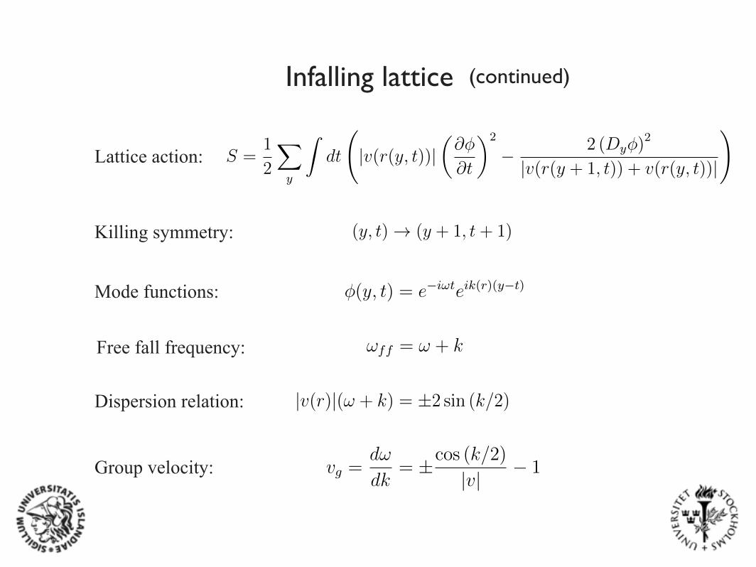
S =

1

2

X

y

ˆdt

|v(r(y, t))|

✓@�

@t

◆2

� 2 (Dy

�)2

|v(r(y + 1, t)) + v(r(y, t))|

!, (4)

6

model, treating the radial direction as a free falling lattice with Planck scale lattice spacing

near the horizon. Rather than work with a two-dimensional model, one can also generalize to

four dimensions, treating the angular directions as continuous spheres, but for our purposes

it turns out to be sufficient to consider the s-wave sector. We will be focusing on near-

horizon physics, so we restrict discussion to the simple case of a Schwarzschild black hole

in asymptotically flat spacetime. Generalization to spacetimes with other asymptotics will

not affect our main conclusions. Furthermore, since we will be considering timescales that

are parametrically short compared to the black hole lifetime, we will model the background

geometry as a static Schwarzschild spacetime.

The starting point for the lattice model is the Schwarzschild metric in Gullstrand-Painlevé

coordinates (in units with G = ~ = c = 1). We define

v(r) = �r

2M

r, (1)

and then the metric is

ds2 = � �1� v2(r)

�dt2 � 2v(r)dt dr + r2d⌦2 ,

where the time coordinate is obtained by adding an r-dependent function to the usual

Schwarzschild time

t = ts

+ 2M

✓� 2

v(r)� log

✓1� v(r)

1 + v(r)

◆◆.

The coordinate transformation is singular on the horizon, as it must be for the Gullstrand-

Painlevé coordinates to be smooth there. We note, however, that this is traded for a coor-

dinate singularity at large r.

For the moment, we take the metric to be of the form (1) inside the horizon of the

black hole r < 2M . This amounts to assuming that neither additional matter stress energy

nor gravitational waves are present inside the horizon. This may appear to be rather a

strong assumption given that the lattice model based on this metric is to be viewed as a

representation of the exact physics described by the holographic theory. However, as we see

later on (towards the end of section III), there is a sense in which the metric (1) behaves as

an attractor in the regulated theory.

The metric is stationary in Gullstrand-Painlevé coordinates so pt

is conserved along a

timelike geodesic. For a particle of unit mass on a radial geodesic we have

5

pt

= �E = � �1� v2(r)� dtd⌧

� v(r)dr

d⌧.



d⌧

◆2

= E2 � 1 + v2(r) .




y = t�ˆ

r

2M

dr0

v(r0),


ds2 = �dt2 + v2(r)dy2 + r2d⌦2 , (2)

with

r(y, t) = 2M

✓1 +

3

4M(y � t)

◆2/3

. (3)
















S =

1

2

X

y

ˆdt

|v(r(y, t))|

✓@�

@t

◆2

� 2 (Dy

�)2

|v(r(y + 1, t)) + v(r(y, t))|

!, (4)

6

Curvature singularity is at y = t - 4M/3 .

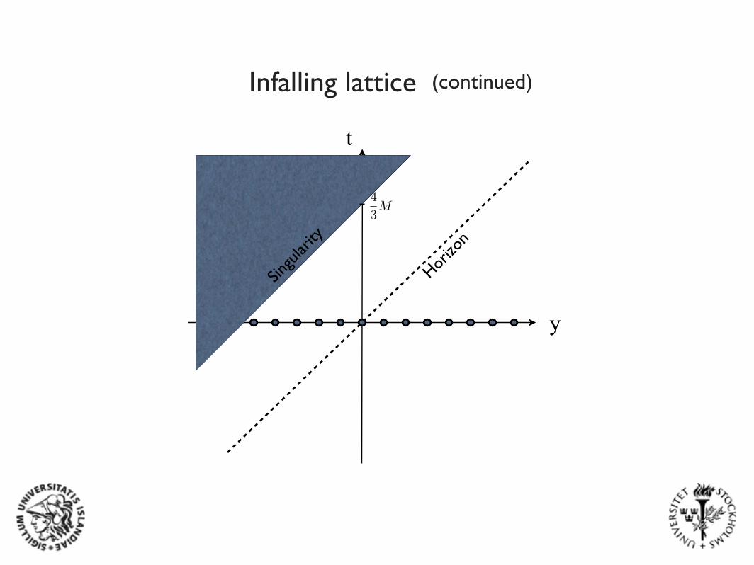
t

y

Singu

larity

4

3M

Horizo

n

Infalling lattice (continued)

Infalling lattice (continued)

Lattice action:

pt

= �E = � �1� v2(r)� dtd⌧

� v(r)dr

d⌧.



d⌧

◆2

= E2 � 1 + v2(r) .




y = t�ˆ

r

2M

dr0

v(r0),


ds2 = �dt2 + v2(r)dy2 + r2d⌦2 , (2)

with

r(y, t) = 2M

✓1 +

3

4M(y � t)

◆2/3

. (3)
















S =

1

2

X

y

ˆdt

|v(r(y, t))|

✓@�

@t

◆2

� 2 (Dy

�)2

|v(r(y + 1, t)) + v(r(y, t))|

!, (4)

6Killing symmetry:

where the difference operator

Dy

� = �(y + 1, t)� �(y, t) .

An attractive feature of this discretization is that the action has a residue of the Killing

symmetry of the Schwarzschild metric

(y, t) ! (y + 1, t+ 1) . (5)

In particular, this allows one to use separation of variables to derive the form of the mode

functions, and determine the lattice dispersion relation. The general form of the mode

function takes the form

�(y, t) = e�i!tf(y � t) , (6)

where the frequency ! may be taken to be any real number. The invariance of the mode

function under

k ! k + 2n⇡, ! ! ! � 2n⇡ (7)

for any integer n allows one to map an arbitrary pair (!, k) into the range

� ⇡ <k ⇡

�1 <!< 1 . (8)

In a WKB approximation, we expand the mode function in terms of wavevectors that

depend on position

�(y, t) = e�i!teik(r)(y�t) . (9)

Plugging (9) into the equation of motion yields the formula obtained by Corley and

Jacobson [3] for the WKB wavevector k(r(y, t))

|v(r)|(! + k) = ±2 sin (k/2) . (10)

This dispersion relation governs the propagation of wavepackets in the (y, t) plane. It can

be solved numerically but the qualitative behavior of solutions can be obtained by simple

graphical analysis based on figure 1. The straight lines in the figure correspond to the left-

hand side of (10) for ! > 0 and three different values of r; outside, inside and at the black

hole horizon, with the slope of the line determined by (1) in each case. Far away from the

black hole v(r) ! 0 and the line approaches horizontal, while deep inside the black hole it

7

Mode functions:


Dy

� = �(y + 1, t)� �(y, t) .



(y, t) ! (y + 1, t+ 1) . (5)




�(y, t) = e�i!tf(y � t) , (6)


function under

k ! k + 2n⇡, ! ! ! � 2n⇡ (7)


� ⇡ <k ⇡

�1 <!< 1 . (8)


depend on position

�(y, t) = e�i!teik(r)(y�t) . (9)



|v(r)|(! + k) = ±2 sin (k/2) . (10)







7

Dispersion relation:


Dy

� = �(y + 1, t)� �(y, t) .



(y, t) ! (y + 1, t+ 1) . (5)




�(y, t) = e�i!tf(y � t) , (6)


function under

k ! k + 2n⇡, ! ! ! � 2n⇡ (7)


� ⇡ <k ⇡

�1 <!< 1 . (8)


depend on position

�(y, t) = e�i!teik(r)(y�t) . (9)



|v(r)|(! + k) = ±2 sin (k/2) . (10)







7

Group velocity:

Figure 2. Interior wavepacket trajectories. The left figure shows the radial position as a function of

the Gulstrand-Painlevé coordinate t. The right figure shows the evolution of the WKB wavevector

k. The blue curves represent the right-moving, horizon skimming mode, which take a scrambling

time to hit the singularity. The red curves represent the left-moving mode. In the figures, M = 100,

! = 1/10.

evolved by free fall from outside the horizon, crossing the horizon at a later time. The

by now standard theory of decoherence (for a textbook treatment see [9]) shows that local

interactions with a large number of exterior degrees of freedom decohere a quantum state,

if given sufficient time. In the case of a black hole this decoherence time is at least of order

the scrambling time [10]. Correlation functions between wavepackets that enter the horizon

separated by less than a scrambling time are not affected by decoherence. However, if our

initial wavepacket is capable of sending a detectable signal to a late time wavepacket that

enters the black hole a scrambling time or more later, then the black hole complementarity

principle will be falsified [11]. In other words, if one takes property #1 as a postulate, then

a violation of property #2 implies violation of black hole complementarity.

It is straightforward to analyze the propagation of such wavepackets, using standard

methods of propagation in dispersive media [12]. The largest amplitude component of the

wavepacket propagates within a timelike cone, bounded by the evolution of trajectories

according to the group velocity of the different Fourier components. The group velocity

with respect to the y � t coordinate of a wavetrain (6) is

vg

=

d!

dk= ±cos (k/2)

|v| � 1 . (11)

Let us begin with a wavepacket just inside the horizon. This is inside the future trapped

region so both signs in (11) correspond to ingoing wavepackets. The minus sign gives rise

10

Free fall frequency:

Figure 1. Graphical solution of the lattice dispersion relation. The straight lines correspond to the

left hand side of 10 for different values of v(r) (and ! > 0).

becomes vertical. For a given value of r, the solutions to the dispersion relation are given by

the points where the corresponding straight line intersects the sinusoidal curves. The choice

of sign in (10) determines whether the mode is right- or left-moving, i.e. moves towards

positive or negative y, respectively, on the infalling lattice with increasing t. For each ! > 0

solution represented in figure 1, there is a corresponding one with ! < 0 (and opposite sign

k). The two branches of solutions are related by complex conjugation and we will restrict

attention to the ! > 0 case.

Far away from the black hole there are four intersection points, corresponding to four

different ! > 0 modes, of which two survive the continuum limit and two are only present

at finite lattice cutoff. Following [3], we denote the modes by +, �, +,s

, and �,s

, and

let the corresponding WKB momenta carry the same subscripts, as indicated in figure 1. Of

these modes, �,s

, is left-moving while the other three are right-moving. The momenta k+

and k� lie outside the fundamental domain in (8) but can be brought inside it by a shift of

the form (7).

Free fall observers, traveling along lines of constant y measure the free-fall frequency

!ff

= ! + k ,

8

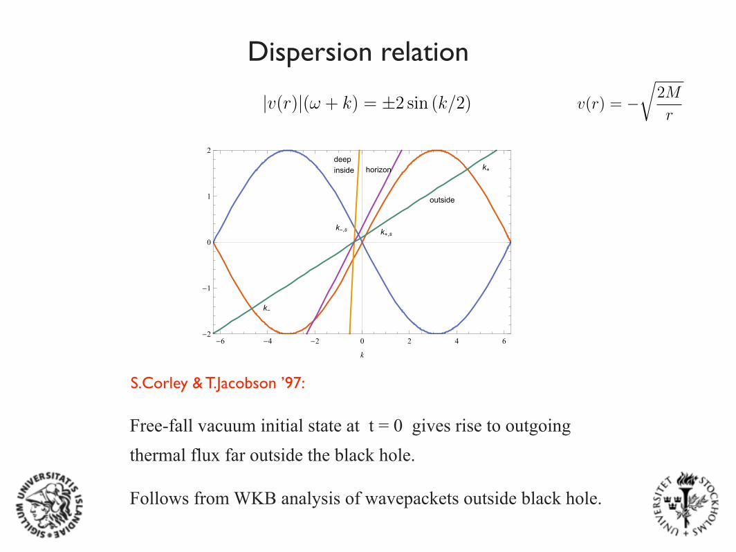
Dispersion relation

outside

horizondeepinside k+

k-

k+,sk-,s

-6 -4 -2 0 2 4 6-2

-1

0

1

2

k













, and �,s

, and


these modes, �,s



the form (7).


!ff

= ! + k ,

8


Dy

� = �(y + 1, t)� �(y, t) .



(y, t) ! (y + 1, t+ 1) . (5)




�(y, t) = e�i!tf(y � t) , (6)


function under

k ! k + 2n⇡, ! ! ! � 2n⇡ (7)


� ⇡ <k ⇡

�1 <!< 1 . (8)


depend on position

�(y, t) = e�i!teik(r)(y�t) . (9)



|v(r)|(! + k) = ±2 sin (k/2) . (10)







7

model, treating the radial direction as a free falling lattice with Planck scale lattice spacing

near the horizon. Rather than work with a two-dimensional model, one can also generalize to

four dimensions, treating the angular directions as continuous spheres, but for our purposes

it turns out to be sufficient to consider the s-wave sector. We will be focusing on near-

horizon physics, so we restrict discussion to the simple case of a Schwarzschild black hole

in asymptotically flat spacetime. Generalization to spacetimes with other asymptotics will

not affect our main conclusions. Furthermore, since we will be considering timescales that

are parametrically short compared to the black hole lifetime, we will model the background

geometry as a static Schwarzschild spacetime.

The starting point for the lattice model is the Schwarzschild metric in Gullstrand-Painlevé

coordinates (in units with G = ~ = c = 1). We define

v(r) = �r

2M

r, (1)

and then the metric is

ds2 = � �1� v2(r)

�dt2 � 2v(r)dt dr + r2d⌦2 ,

where the time coordinate is obtained by adding an r-dependent function to the usual

Schwarzschild time

t = ts

+ 2M

✓� 2

v(r)� log

✓1� v(r)

1 + v(r)

◆◆.

The coordinate transformation is singular on the horizon, as it must be for the Gullstrand-

Painlevé coordinates to be smooth there. We note, however, that this is traded for a coor-

dinate singularity at large r.

For the moment, we take the metric to be of the form (1) inside the horizon of the

black hole r < 2M . This amounts to assuming that neither additional matter stress energy

nor gravitational waves are present inside the horizon. This may appear to be rather a

strong assumption given that the lattice model based on this metric is to be viewed as a

representation of the exact physics described by the holographic theory. However, as we see

later on (towards the end of section III), there is a sense in which the metric (1) behaves as

an attractor in the regulated theory.

The metric is stationary in Gullstrand-Painlevé coordinates so pt

is conserved along a

timelike geodesic. For a particle of unit mass on a radial geodesic we have

5

Free-fall vacuum initial state at t = 0 gives rise to outgoing thermal flux far outside the black hole.

S.Corley & T.Jacobson ’97:

Follows from WKB analysis of wavepackets outside black hole.

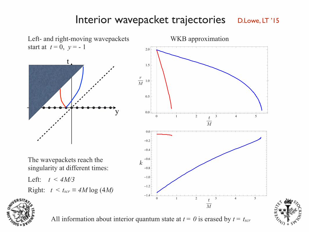
Interior wavepacket trajectories

Left- and right-moving wavepackets start at t = 0, y = - 1

y

t

� � � � � ��

��

��

��

��

�

�





! = 1/10.
















vg

=

d!

dk= ±cos (k/2)

|v| � 1 . (11)



10

t

M

r

M

� � � � � �-��

-��

-��

-��

-��

-��

-��

��

�





! = 1/10.
















vg

=

d!

dk= ±cos (k/2)

|v| � 1 . (11)



10

t

M

k

WKB approximation

The wavepackets reach the singularity at different times:

Left: t < 4M/3 Right: t < tscr ≡ 4M log (4M)

All information about interior quantum state at t = 0 is erased by t = tscr

D.Lowe, LT ’15

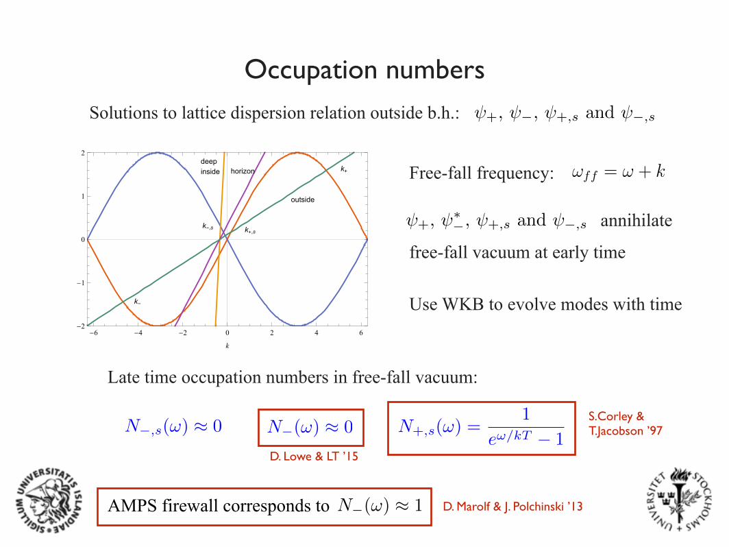
Occupation numbersSolutions to lattice dispersion relation outside b.h.:

Use WKB to evolve modes with time

Free-fall frequency:













, and �,s

, and


these modes, �,s



the form (7).


!ff

= ! + k ,

8outside

horizondeepinside k+

k-

k+,sk-,s

-6 -4 -2 0 2 4 6-2

-1

0

1

2

k













, and �,s

, and


these modes, �,s



the form (7).


!ff

= ! + k ,

8

+, �, +,s and �,s

free-fall vacuum at early time

+, ⇤�, +,s and �,s annihilate

Late time occupation numbers in free-fall vacuum:

N+,s(!) =1

e!/kT � 1N�,s(!) ⇡ 0 N�(!) ⇡ 0

AMPS firewall corresponds to N�(!) ⇡ 1

S.Corley & T.Jacobson ’97

D. Lowe & LT ’15

D. Marolf & J. Polchinski ’13

The information paradox highlights the incompatibility between general relativity (locality + equivalence principle) and quantum physics (unitarity).

Gauge theory - gravity correspondence implies unitary black hole evolution.

Black hole complementarity provides a "phenomenological" description, which preserves unitarity and the equivalence principle, but requires giving up locality.

Typical infalling observers do not see drama on their way towards a black hole formed from a generic pure state. (Special pure states, as well as special observers, exist for which this is not true.)

An approximate description of observers in the black hole interior can be given in terms of an effective field theory, defined on a limited set of time slices, such that no drama is seen until near the singularity.

A spin system with a nonlocal pairwise interaction provides a toy model for the holographic description of the black hole interior.

Evolution with respect to the bulk effective Hamiltonian is dual to mean field evolution in the holographic model.

Decoherence time for an infalling lab matches black hole scrambling time.

Summary

Documents

Introduction to Black Hole Informatics