Embed Size (px)
Citation preview

Introduction to Biostatistics and Bioinformatics
Hypothesis Testing I
This Lecture
By Judy Zhong
Assistant Professor
Division of Biostatistics
Department of Population Health
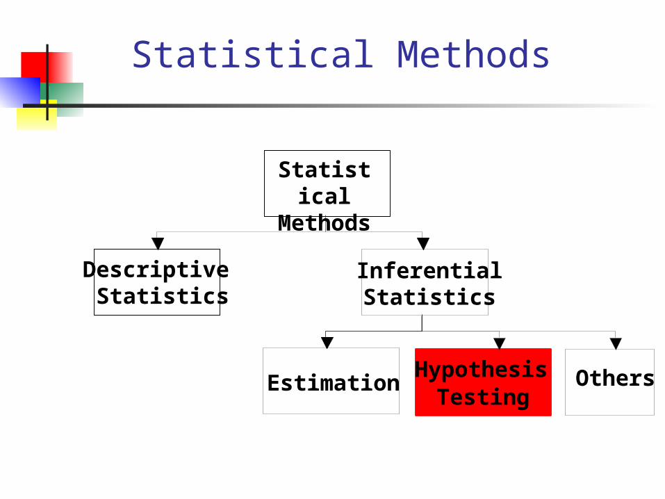
Statistical Methods
StatisticalMethods
Descriptive Statistics
InferentialStatistics
EstimationHypothesis
TestingOthers
Hypothesis testing
Research hypotheses are conjectures or suppositions that motivate the research
Statistical hypotheses restate the research hypotheses to be addressed by statistical techniques.
Formally, a statistical hypothesis testing problem includes two hypothesis Null hypothesis (H0) Alternative hypothesis (Ha, H1)
In statistical hypothesis testing, we start off believing the null hypothesis, and see if the data provide enough evidence to abandon our belief in H0 in favor of Ha
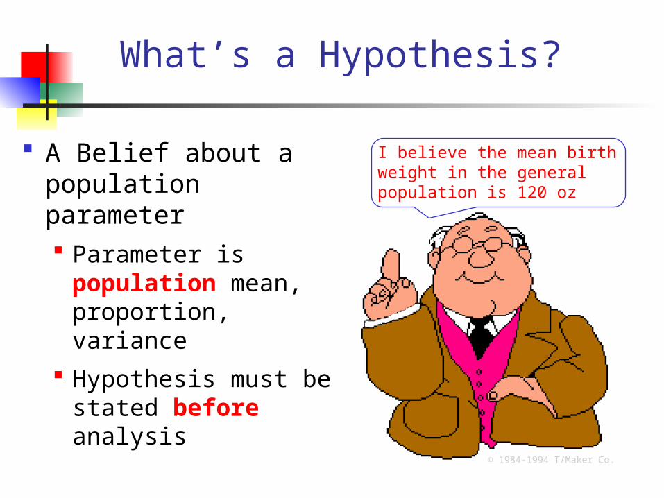
What’s a Hypothesis?
A Belief about a population parameter Parameter is population
mean, proportion, variance
Hypothesis must be stated before analysis
I believe the mean birth weight in the general population is 120 oz
© 1984-1994 T/Maker Co.
Birth Weight Example
Average birth weight in the general population is 120 oz. You take a sample of 100 babies born in the hospital you work at
(that is located in a low-SES area), and find that the sample mean birth weight is 115 oz.
You wonder:
is this observed difference merely due to chance OR
is the mean birth weight of SES babies indeed lower than that in the general population?
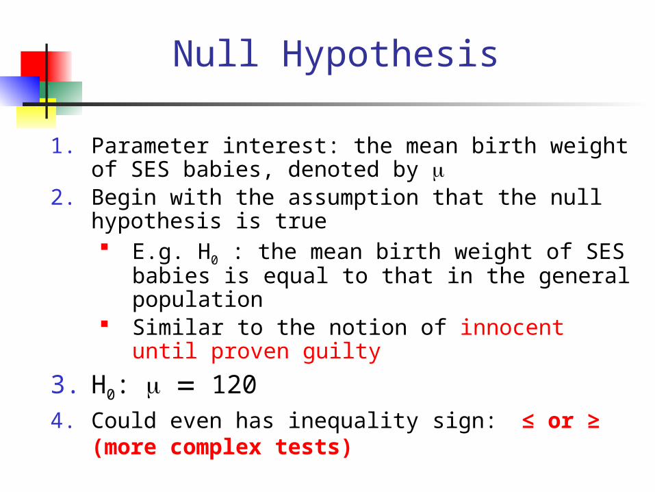
Null Hypothesis
1. Parameter interest: the mean birth weight of SES babies, denoted by
2. Begin with the assumption that the null hypothesis is true E.g. H0 : the mean birth weight of SES babies is
equal to that in the general population Similar to the notion of innocent until proven guilty
3. H0: 1204. Could even has inequality sign: ≤ or ≥ (more complex
tests)
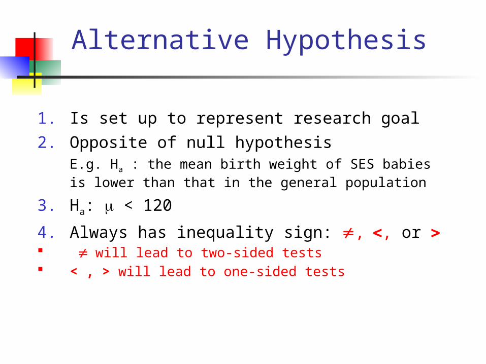
Alternative Hypothesis
1. Is set up to represent research goal
2. Opposite of null hypothesisE.g. Ha : the mean birth weight of SES babies is lower than that in the general population
3. Ha: < 120
4. Always has inequality sign: ,, or will lead to two-sided tests < , > will lead to one-sided tests
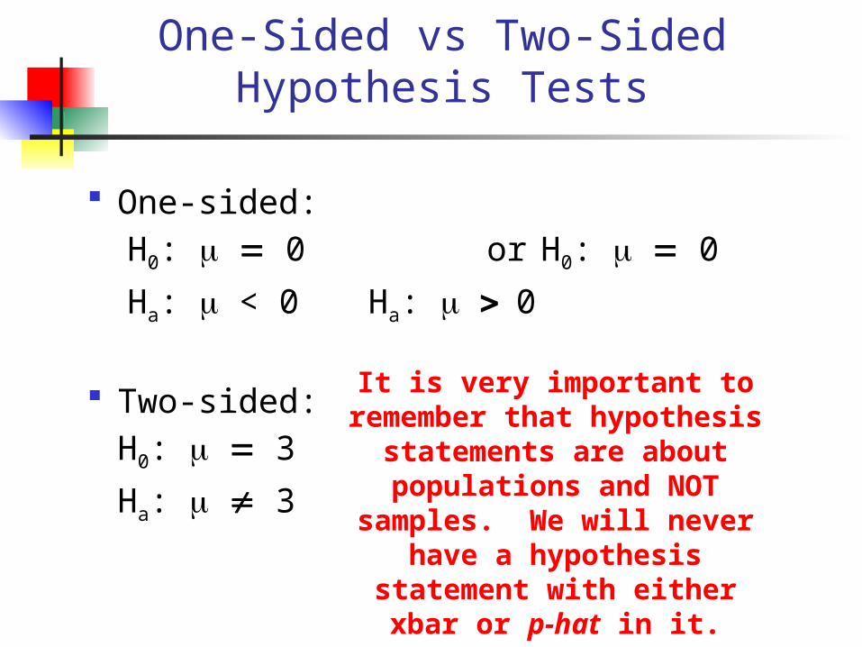
One-Sided vs Two-Sided Hypothesis Tests
One-sided:
H0: 0 or H0: 0
Ha: < 0 Ha: 0
Two-sided:
H0: 3
Ha: 3
It is very important to remember that hypothesis
statements are about populations and NOT
samples. We will never have a hypothesis statement with either xbar or p-hat in it.
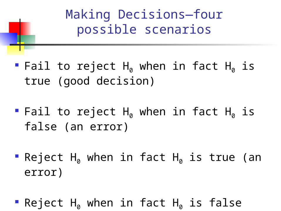
Making Decisions—four possible scenarios
Fail to reject H0 when in fact H0 is true (good decision)
Fail to reject H0 when in fact H0 is false (an error)
Reject H0 when in fact H0 is true (an error)
Reject H0 when in fact H0 is false (good decision)
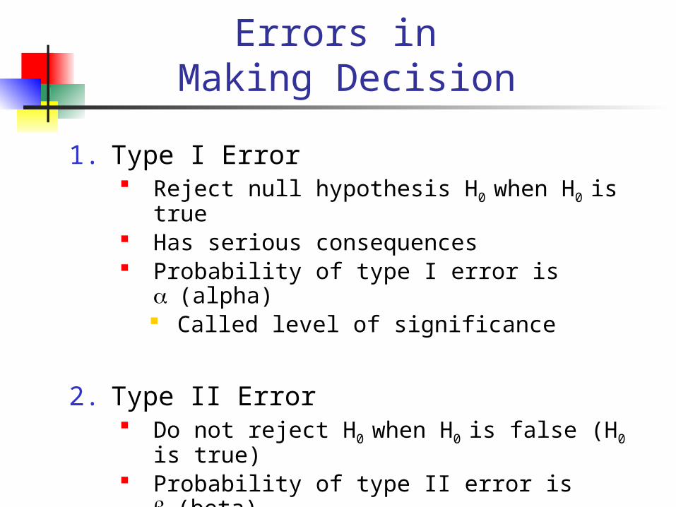
Errors in Making Decision
1. Type I Error Reject null hypothesis H0 when H0 is true Has serious consequences Probability of type I error is (alpha)
Called level of significance
2. Type II Error Do not reject H0 when H0 is false (H0 is true) Probability of type II error is (beta)
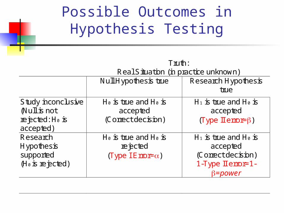
Possible Outcomes in Hypothesis Testing
Truth: Real Situation (in practice unknown)
Null Hypothesis true Research Hypothesis true
Study inconclusive (Null is not rejected: H0 is accepted)
H0 is true and H0 is accepted
(Correct decision)
H1 is true and H0 is accepted
(Type II error=)
Research Hypothesis supported (H0 is rejected)
H0 is true and H0 is rejected
(Type I Error=)
H1 is true and H0 is accepted
(Correct decision) 1-Type II error=1-
=power
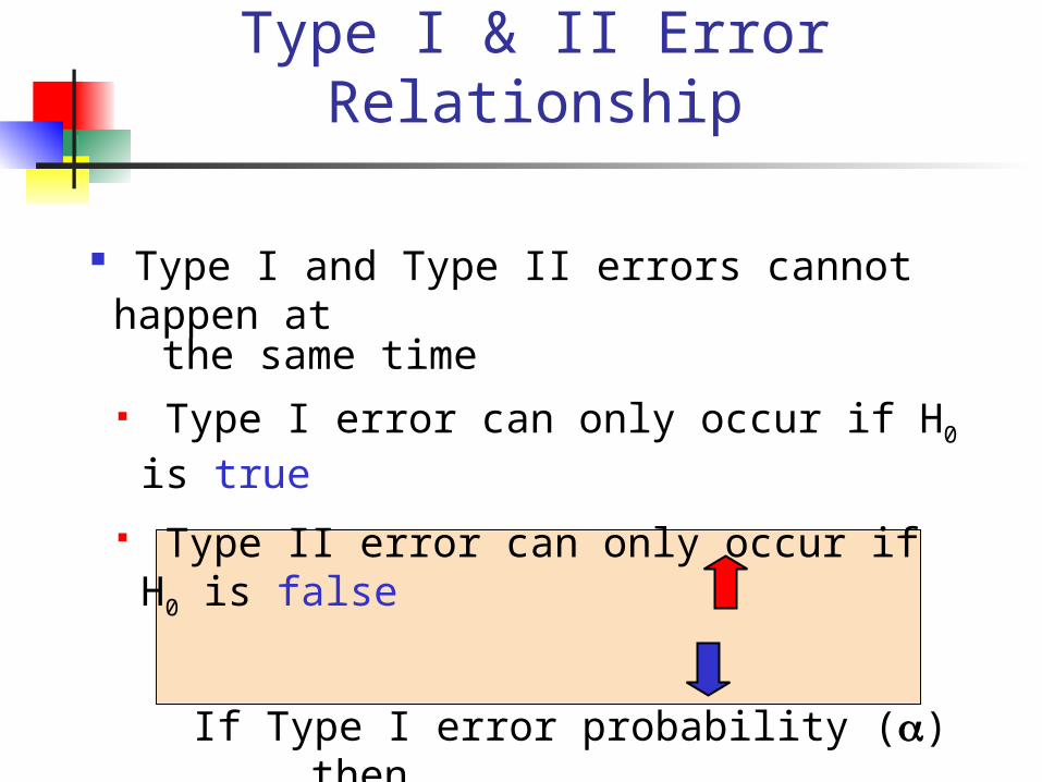
Type I & II Error Relationship
Type I and Type II errors cannot happen at the same time
Type I error can only occur if H0 is true
Type II error can only occur if H0 is false
If Type I error probability () , then
Type II error probability ()
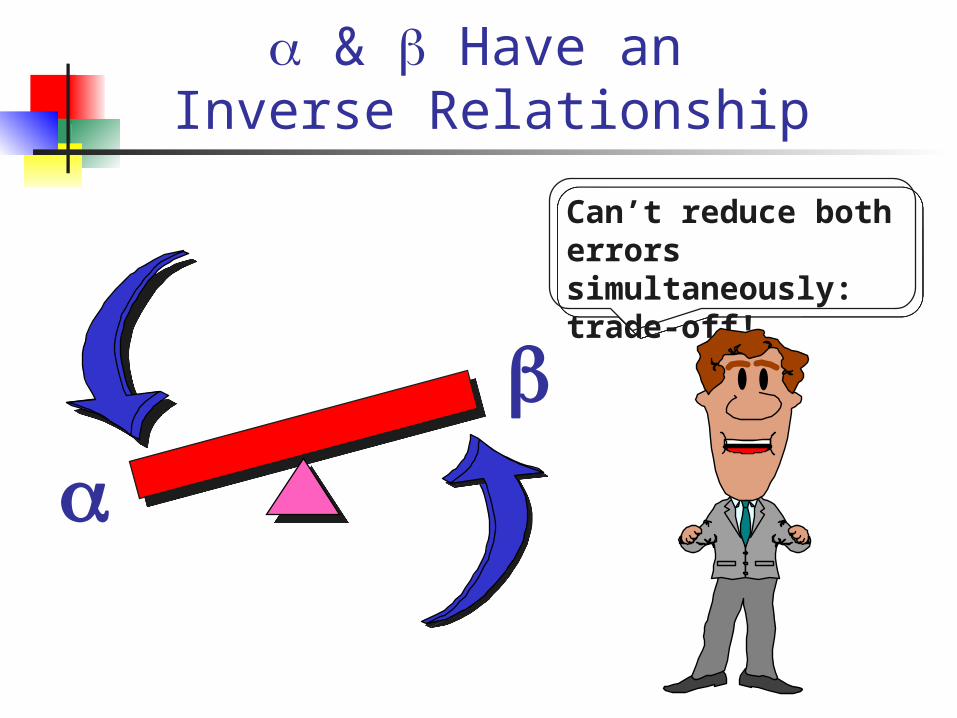
& Have an Inverse Relationship
Can’t reduce both errors simultaneously:
trade-off!
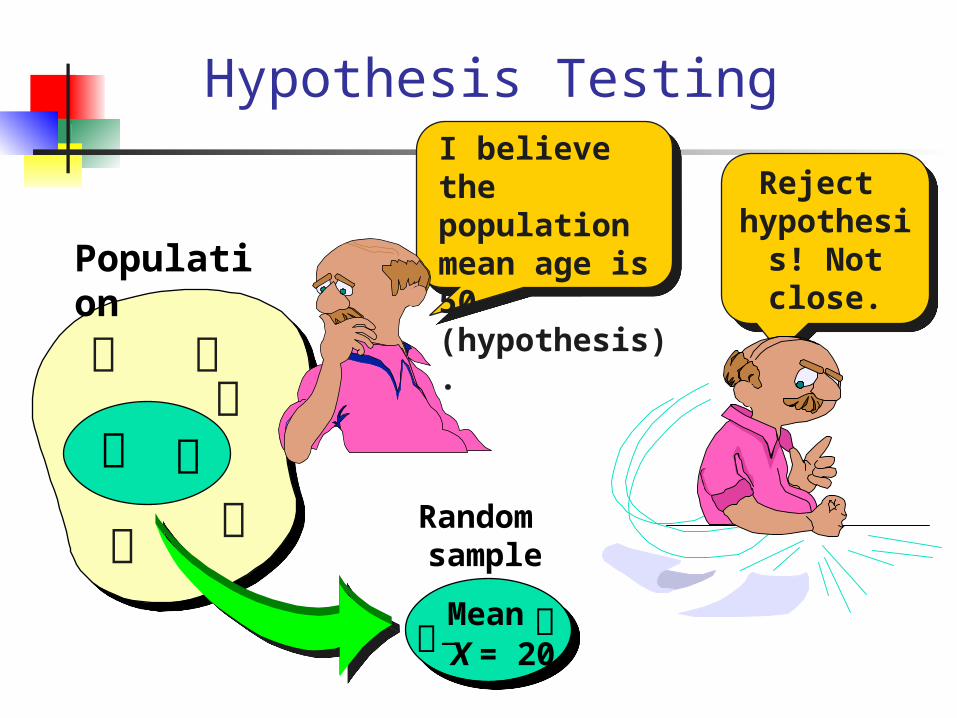
Hypothesis Testing
Population
I believe the population mean age is 50 (hypothesis).
Mean X = 20
Reject hypothesis! Not close.
Reject hypothesis! Not close.
Random sample
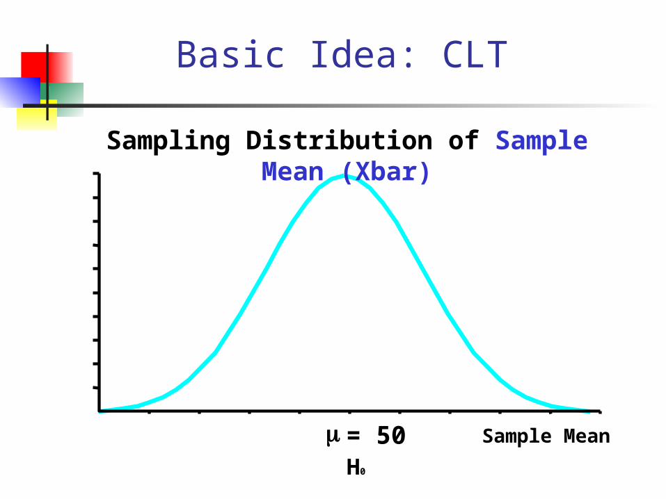
Basic Idea: CLT
Sample Meanm = 50
Sampling Distribution of Sample Mean (Xbar)
H0
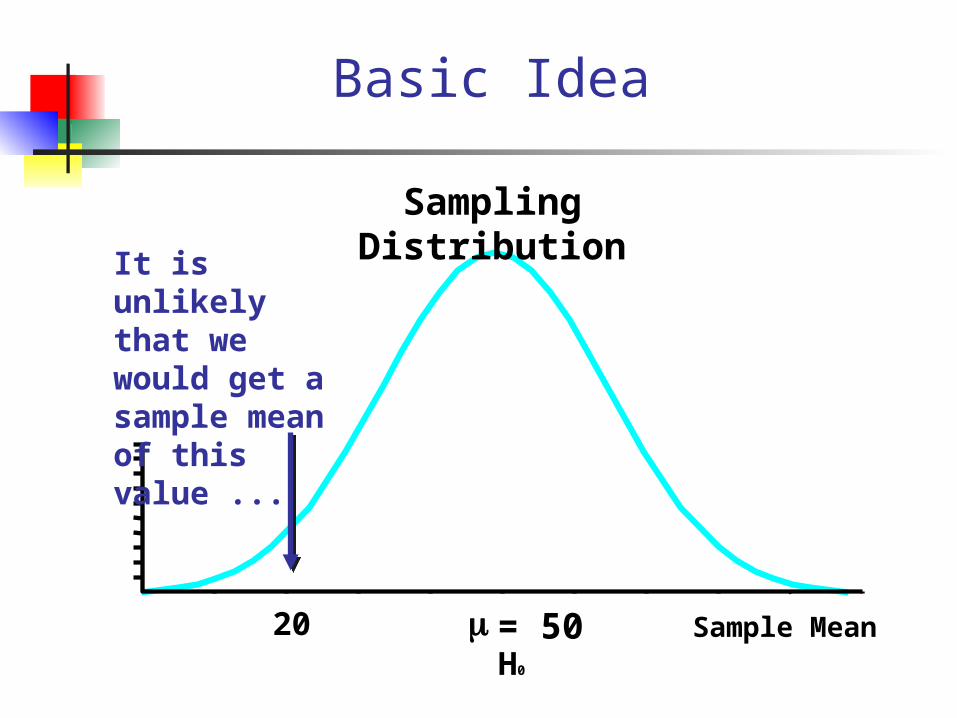
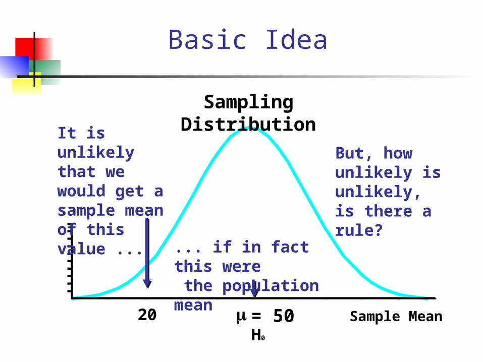
Basic Idea
Sample Meanm = 50
Sampling Distribution
It is unlikely that we would get a sample mean of this value ...
20H0
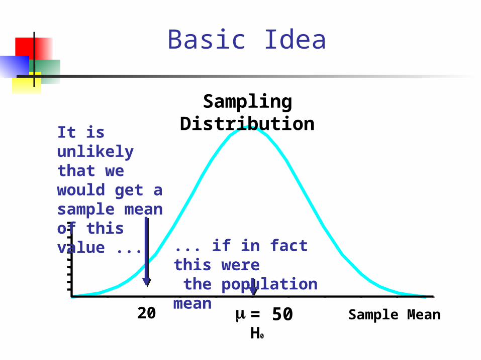
Basic Idea
Sample Meanm = 50
Sampling Distribution
It is unlikely that we would get a sample mean of this value ...
... if in fact this were the population mean
20H0
Basic Idea
Sample Meanm = 50
Sampling Distribution
It is unlikely that we would get a sample mean of this value ...
... if in fact this were the population mean
But, how unlikely is unlikely, is there a rule?
20H0
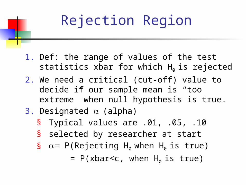
Rejection Region
1. Def: the range of values of the test statistics xbar for which H0 is rejected
2. We need a critical (cut-off) value to decide if our sample mean is “too extreme” when null hypothesis is true.
3. Designated (alpha)§ Typical values are .01, .05, .10§ selected by researcher at start
§ = P(Rejecting H0 when H0 is true)
= P(xbar<c, when H0 is true)
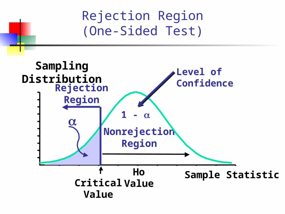
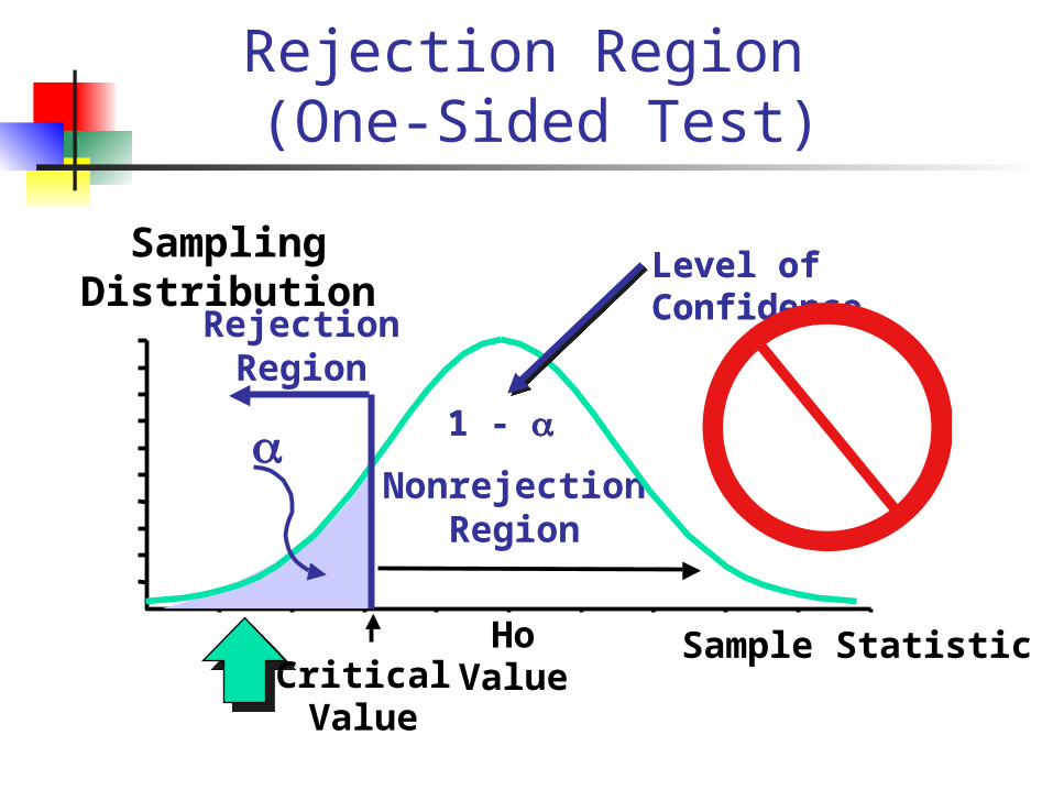
Rejection Region (One-Sided Test)
Sampling Distribution
HoValueCritical
Value
a
Sample Statistic
RejectionRegion
NonrejectionRegion
1 -
Level of Confidence
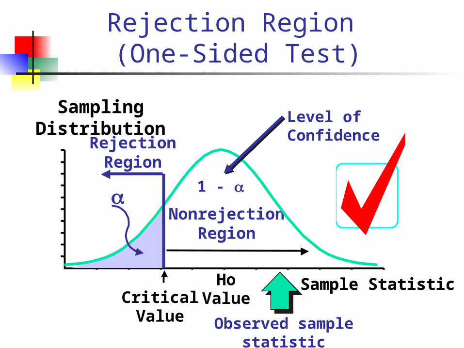
Rejection Region (One-Sided Test)
Sample Statistic
Sampling Distribution
Observed sample statistic
HoValueCritical
Value
a
Sample Statistic
RejectionRegion
NonrejectionRegion
1 -
Level of Confidence
Rejection Region (One-Sided Test)
Sampling Distribution
1 -
Level of Confidence
HoValueCritical
Value
a
Sample Statistic
RejectionRegion
NonrejectionRegion
1 -
Level of Confidence
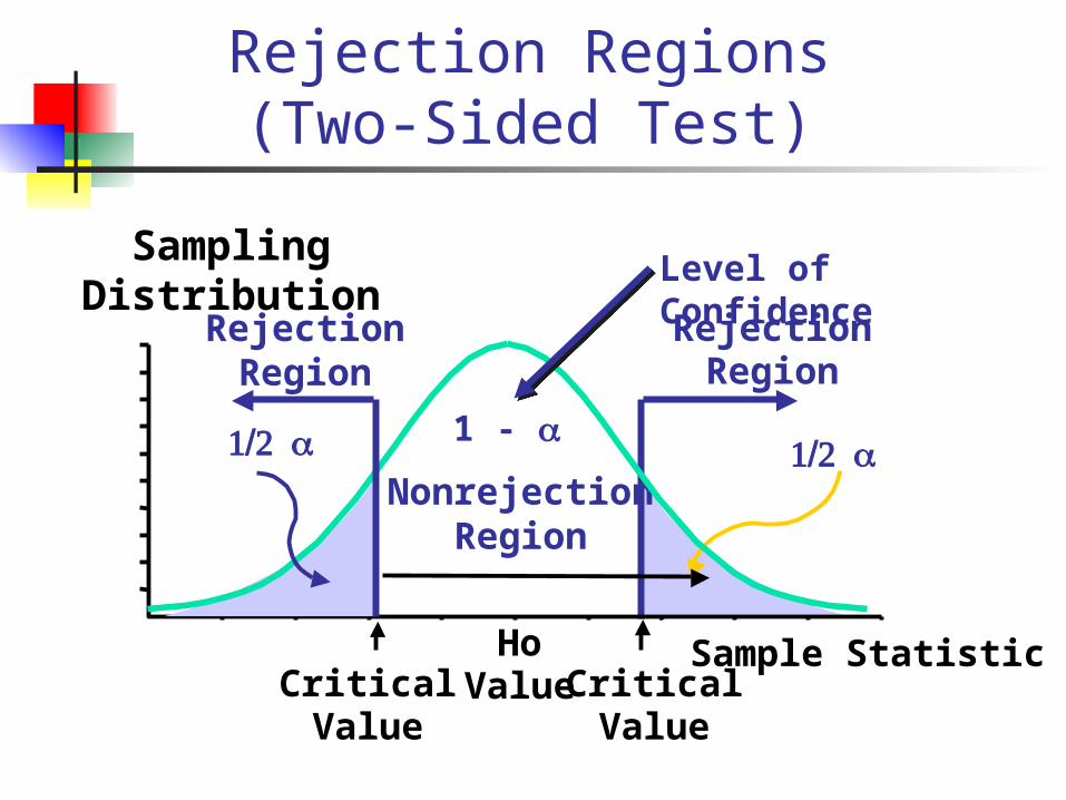
Rejection Regions (Two-Sided Test)
Sampling Distribution
CriticalValue
1/2 a
RejectionRegion
HoValueCritical
Value
1/2 a
Sample Statistic
RejectionRegion
NonrejectionRegion
1 -
Level of Confidence
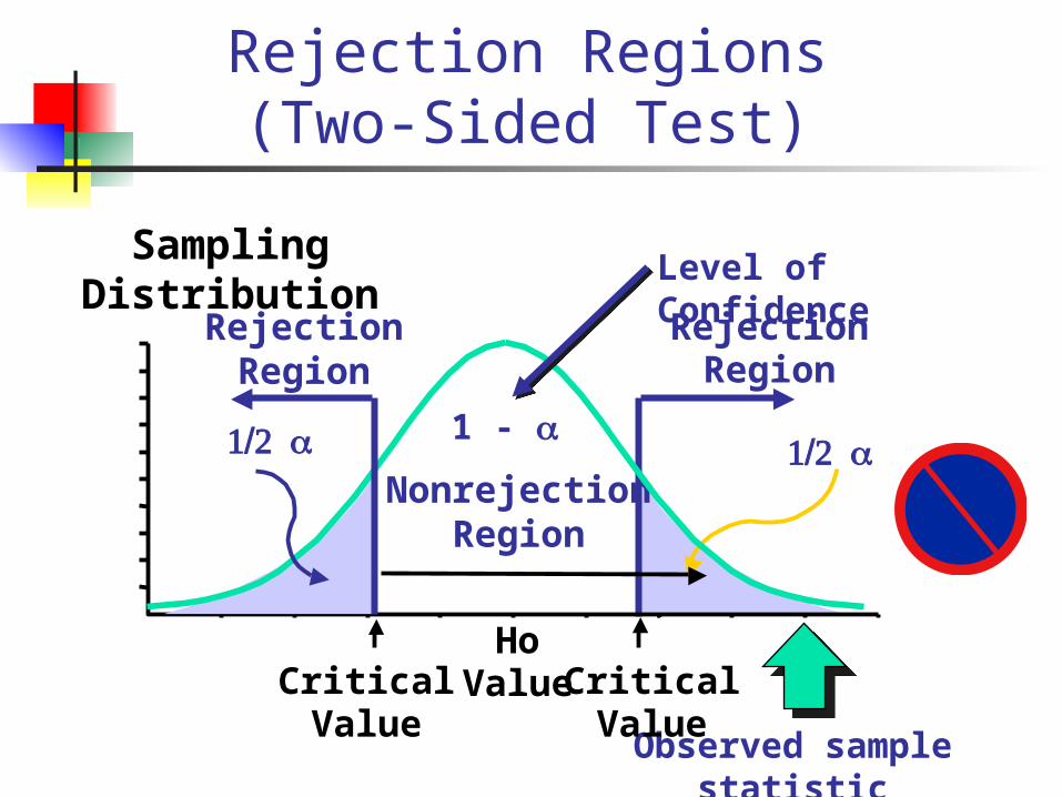
Rejection Regions (Two-Sided Test)
Sampling Distribution
Observed sample statistic
CriticalValue
1/2 a
RejectionRegion
HoValueCritical
Value
1/2 a
RejectionRegion
NonrejectionRegion
1 -
Level of Confidence
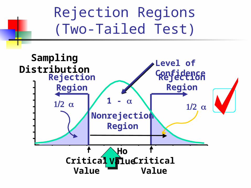
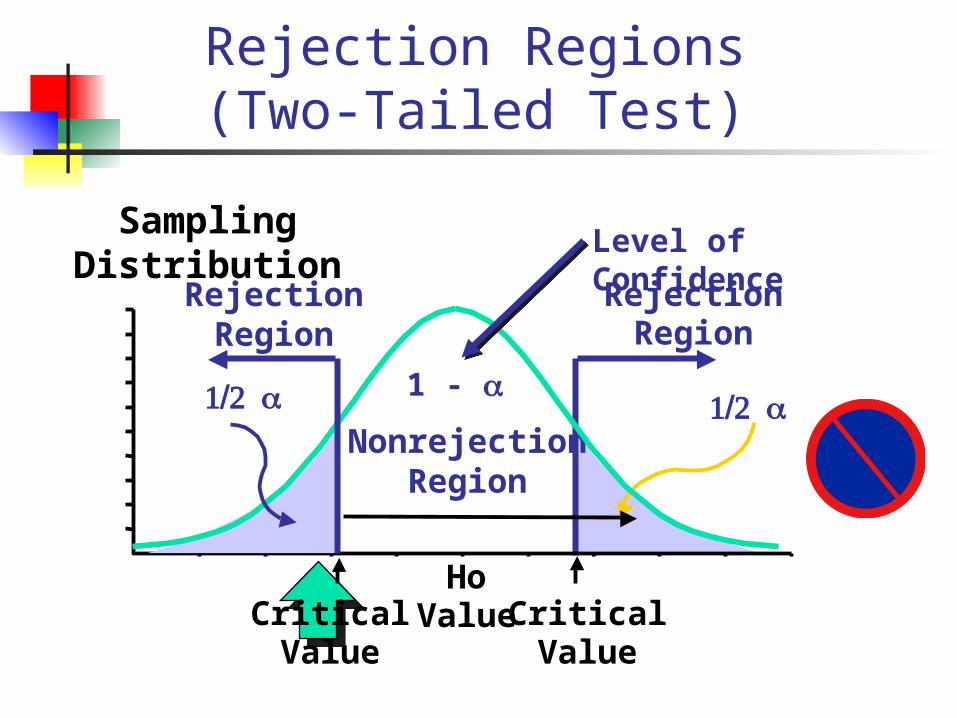
Rejection Regions (Two-Tailed Test)
Sampling Distribution
CriticalValue
1/2 a
RejectionRegion
HoValueCritical
Value
1/2 a
RejectionRegion
NonrejectionRegion
1 -
Level of Confidence
Rejection Regions (Two-Tailed Test)
Sampling Distribution
CriticalValue
1/2 a
RejectionRegion
HoValueCritical
Value
1/2 a
RejectionRegion
NonrejectionRegion
1 -
Level of Confidence
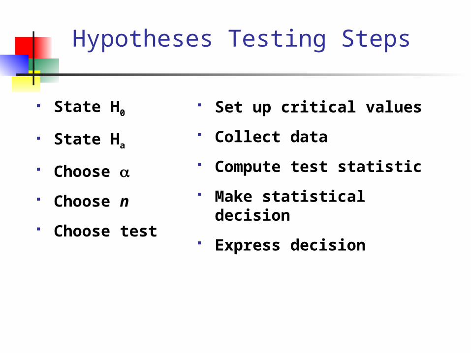
Hypotheses Testing Steps
Set up critical values
Collect data
Compute test statistic
Make statistical decision
Express decision
State H0
State Ha
Choose
Choose n
Choose test
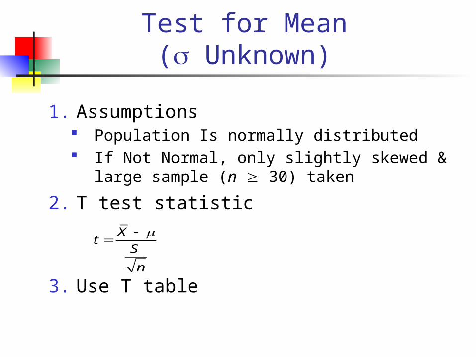
Test for Mean ( Unknown)
1. Assumptions Population Is normally distributed If Not Normal, only slightly skewed & large sample
(n 30) taken
2. T test statistic
3. Use T table
t X
S
n
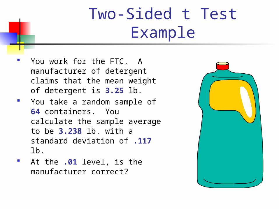
Two-Sided t TestExample
You work for the FTC. A manufacturer of detergent claims that the mean weight of detergent is 3.25 lb.
You take a random sample of 64 containers. You calculate the sample average to be 3.238 lb. with a standard deviation of .117 lb.
At the .01 level, is the manufacturer correct?
3.25 lb.
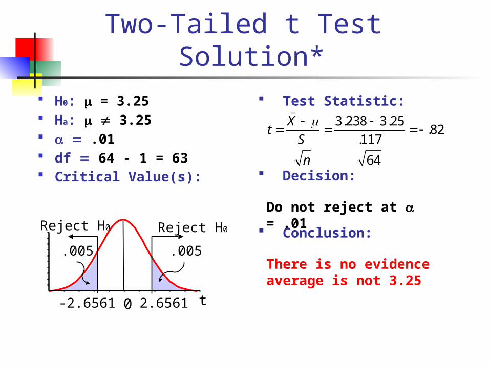
Two-Tailed t Test Solution*
H0: = 3.25 Ha: 3.25 .01 df 64 - 1 = 63 Critical Value(s):
Test Statistic:
Decision:
Conclusion:
t X
S
n
3.238 3.25
.117
64
.82
Do not reject at = .01
There is no evidence average is not 3.25
t0 2.6561-2.6561
.005
Reject H0
.005
Reject H0
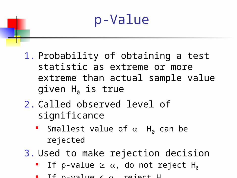
p-Value
1. Probability of obtaining a test statistic as extreme or more extreme than actual sample value given H0 is true
2. Called observed level of significance Smallest value of H0 can be rejected
3. Used to make rejection decision If p-value , do not reject H0
If p-value < , reject H0
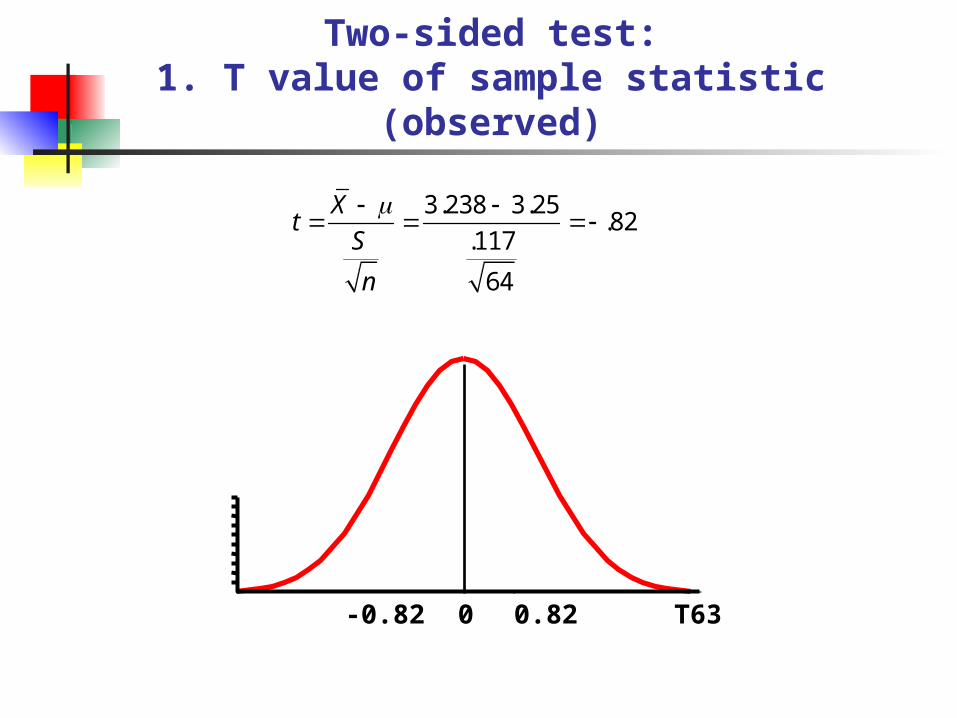
Two-sided test:1. T value of sample statistic (observed)
T630 0.82-0.82
t X
S
n
3.238 3.25
.117
64
.82
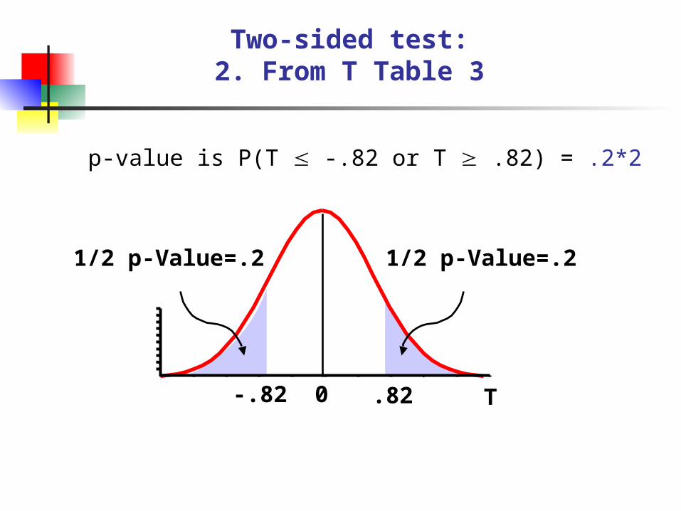
Two-sided test:2. From T Table 3
p-value is P(T -.82 or T .82) = .2*2
T0 .82-.82
1/2 p-Value=.2 1/2 p-Value=.2
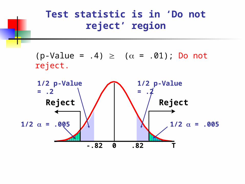
Test statistic is in ‘Do not reject’ region
(p-Value = .4) ( = .01); Do not reject.
0 .82-.82 T
RejectReject
1/2 p-Value = .21/2 p-Value = .2
1/2 = .0051/2 = .005
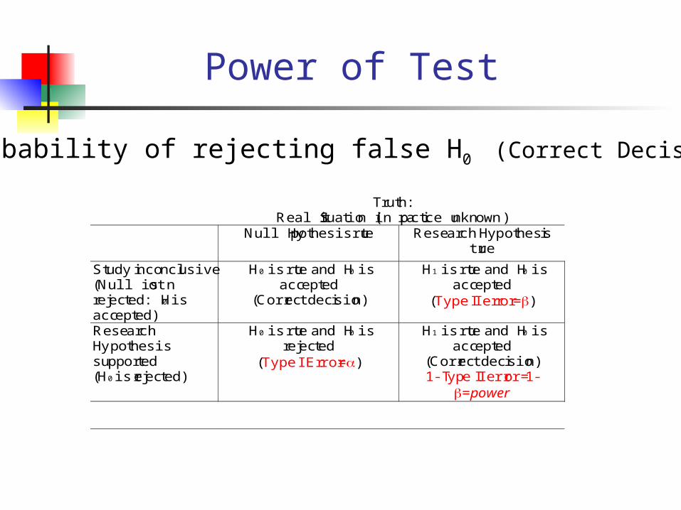
Power of Test
Truth:Real Situation (in practice unknown)
Null Hypothesis true Research Hypothesistrue
Study inconclusive(Null is notrejected: H0 isaccepted)
H0 is true and H0 isaccepted
(Correct decision)
H1 is true and H0 isaccepted
(Type II error=)
ResearchHypothesissupported(H0 is rejected)
H0 is true and H0 isrejected
(Type I Error=)
H1 is true and H0 isaccepted
(Correct decision)1-Type II error=1-
=power
Probability of rejecting false H0 (Correct Decision)
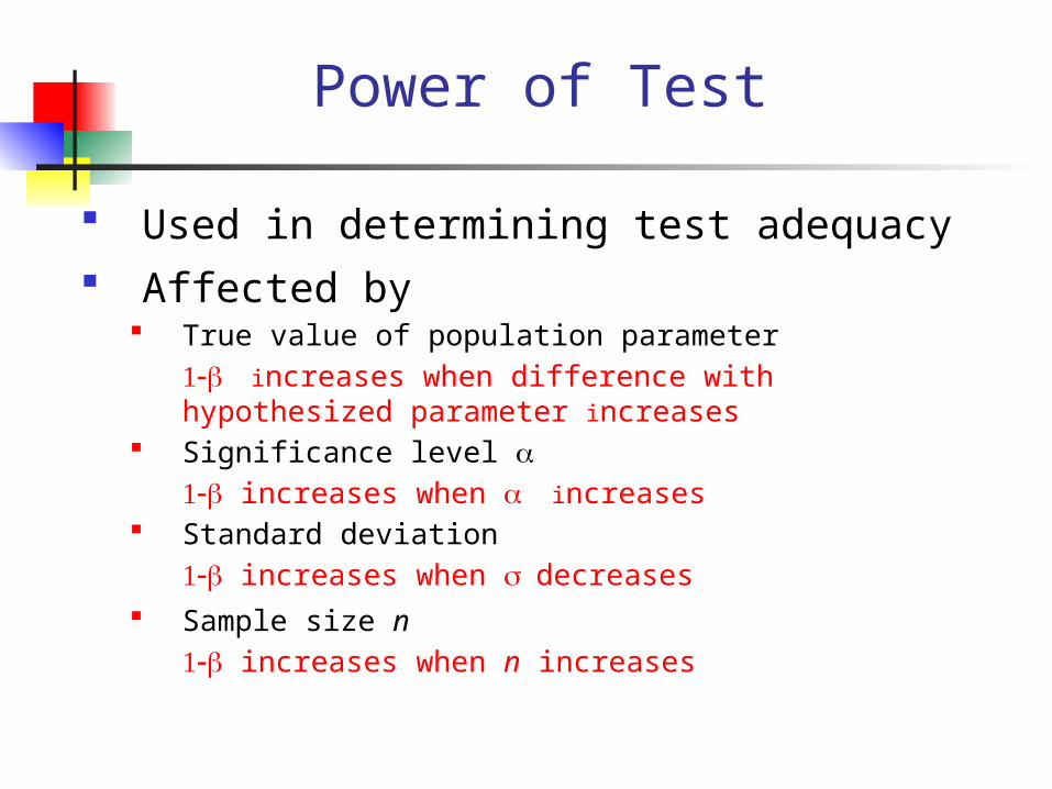
Power of Test
Used in determining test adequacy Affected by
True value of population parameter
1- increases when difference with hypothesized parameter increases
Significance level 1- increases when increases
Standard deviation
1- increases when decreases
Sample size n
1- increases when n increases
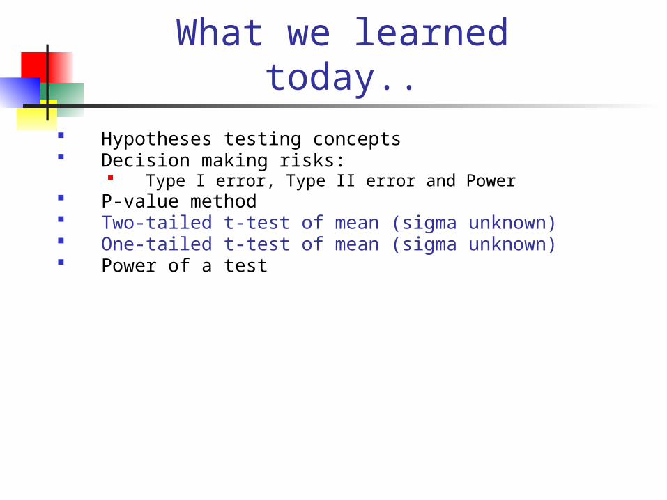
What we learned today..
Hypotheses testing concepts Decision making risks:
Type I error, Type II error and Power P-value method Two-tailed t-test of mean (sigma unknown) One-tailed t-test of mean (sigma unknown) Power of a test