Embed Size (px)
Citation preview

1
1
Introduction to Big Data
Daniel [email protected]
This lecture is an introduction to big data computing, illustrated with Hadoop and Spark.

2
2
Context
We generate more and more dataIndividuals and companies
Kb → Mb → Gb → Tb → Pb → Eb → Zb → Yb → ???
Few numbersIn 2013, Twitter generates 7 Tb per day and Facebook 10 Tb
The square kilometre array radio telescopeProducts 7 Pb of raw data per second, 50 Tb of analyzed data per day
Airbus generates 40 Tb for each plane test
Created digital data worldwide2010 : 1,2 Zb / 2011 : 1,8 Zb / 2012 : 2,8 Zb / 2020 : 40 Zb
90 % of data were created in the last 2 years
Today's digital applications are generating more and more data. These data may be generated by individuals (through social networks) or companies.
Examples are Twitter and Facebook who analyze the behavior of their users, large scientific equipments like the square kilometre array radio telescope.
Another example I have been working on comes from Airbus. When they have designed and built a new plane, during the test phase, the plane is equipped with a huge set of captors which monitor everything. Each test flight generates about 40 TB of data and they run several test flights per week over a year.
The amount of data generated worldwide becomes so large and it is exponential.

3
3
Context
Many data sourcesMultiplication of computing devices and connected electronic equipments
Geolocation, e-commerce, social networks, logs, internet of things …
Many data formatsStructured and unstructured data
It is important to remember that these data are coming from many sources, with the multiplication of devices (personal computers, phones, tablets) and the development of cloud applications.
These diverse sources generate data in many different formats. Such format can be structured (with XML, Json ..) or unstructured (like textual data).

4
4
Applications domains
Scientific applications (biology, climate …)
E-commerce (recommendation)
Equipment supervision (e.g. energy)
Predictive maintenance (e.g. airlines)
EspionageThe NSA has built an infrastructure that allows it to intercept almost everything. With this capability, the vast majority of human communications are automatically ingested without targeting. E Snowden
These data are generated and used (analyzed) in many application domains
Scientific application : biology (genomic) or climate (weather prediction)
E-commerce : profiling users for product recommendation
Equipment supervision : energy where they profile consumption
Predictive maintenance : for instance in the airline industry, they monitor each flight with captors embedded in planes. When a failure occurs, they analyze the monitored data before the failure to identify symptoms that preceded the failure. Therefore, by analyzing data from each flight, they can detect such symptoms before a failure occurs and anticipate a maintenance to prevent the failure.
Espionage : E. Snowden revealed that the NSA was analyzing data from so many sources in a wish to control everybody.

5
5
New jobs
Data ScientistManager : know how to define objectives and identify the value of information
Statistician : know how to use mathematics to classify, group and analyze information
HPC specialist : parallelism is key
IT specialist : know how to develop, parameterize, deploy tools
The field of big data is generating many jobs:
- manager who are dealing with high level objectives
- mathematicians who are analyzing and modeling data
- HPC specialists who know how to improve performance
- IT specialists who master the infrastructure (hardware and software)

6
6
Computing infrastructures
The reduced cost of infrastructures
Main actors (Google, Facebook, Yahoo, Amazon …) developed frameworks for storing and processing data
We generally consider that we enter the Big Data world when processing cannot be performed with a single computer
Decades ago, data treatments were performed by a single computer, a multiprocessor machine if computing power was required.
Two main evolutions modified that:
- new applications which require huge computing power
- the reduced code of hardware (mainly servers and networks), leading to the development of clusters (a huge set of interconnected servers).
A cluster is a set of interconnected servers which are exploited by a distributed operating system in order to give the illusion of a giant computer.
The main actors of the field developed such distributed operating system frameworks to implement a sort of giant computer for storing and processing data.
We generally consider that we enter the Big Data world when processing cannot be performed with a single computer (even a large one) and when a cluster is required.

7
7
Definition of Big Data
DefinitionRapid treatment of large data volumes, that could hardly be handled with traditional techniques and tools
The three V of Big DataVolume
Velocity
Variety
Two additional VVeracity
Value
One (among many) definition of Big Data is the rapid treatment of large data volumes that could hardly be handled with traditional techniques and tools (e.g. a database system on a single computer).
In the field, people are talking about the 3 V which characterize Big Data:
- Volume : dealing with very large data volumes
- Velocity : treatment should be fast enough
- Variety : data may be of very different types
Sometimes, they add 2 additional V :
- Veracity : big data may also consider the trust we have into the handled data
- Value : it may also consider the value of the data
And may be at the time of today, they added again other Vs.

8
8
General approach
Main principle : divide and conquerDistribute IO and computing between several devices
request
request
sub-request
sub-request
Traditional centralized technology
request
sub-request
sub-request
SR SR SR
SR SR SR
Bigdata distributed technology
The general approach used to efficiently treat very large datasets is to apply a well known principle called "divide and conquer".
The principle is to divide a task into several sub-tasks which can be distributed on distributed computers, therefore benefiting from parallel IO (reads from different disks) and/or parallel computation (on different processors).
Figure top : in a traditional centralized setting, a request or task is executed on one computer.
Figure middle : a request can be divided into 2 sub requests executed in parallel on 2 separate computers.
Figure bottom : the request can be divided into many sub-requests scheduled on many computers. This can be done if the initial request is sufficiently large.
Notice here that in this general principle, we don't precise how data are moved to the computers where sub-requests are executed.

9
9
Solutions
Two main families of solutionsProcessing in batch mode (e.g. Hadoop)
Data are initially stored in the cluster
Various requests are executed on these data
Data don't change / requests change
Processing in streaming mode (e.g. Storm)Data are continuously arriving in streaming mode
Treatments are executed on the fly on these data
Data change / Requests don't change
} This lecture
The previous general principle leads to 2 main families of solution.
Processing in batch mode (Hadoop is an example). Data are initially stored on the computers' disks. For instance a very large dataset is divided into blocks and the blocks are distributed on the machines. Then, various requests can be issued to analyze the data. Such a request is divided into sub-requests which will handle the blocks on the different machines (in parallel). What is important here is that the data are installed in the cluster (installed means here that data don't change, they are here to be read and analyzed, not modified) and that many requests can be issued on the same dataset.
Processing in streaming mode (Storm is an example). Data are continuously arriving in streaming mode. Treatments are decomposed in tasks that are deployed in the cluster.
In this lecture, we focus on batch mode processing.

10
10
The map-reduce principle
We have to manage many stores around the worldA large document registers all the sales
For each sale : day – city – product - price
Objective : compute the total of sales per store
The traditional methodA Hashtable memorizes the total for each store (<city, total>)
We iterate through all recordsFor each record, if we find the city in the Hashtable, we add the price
Let's use an illustrative example.
We consider the management of a set of stores geographically distributed.
A large document gathers records of all the sales, with for each sale : the day, the city, the product code and the price.
One request we may issue on the document is to compute for each store the total of the sales.
The traditional method is a sequential program which iterates over all the records. A hashtable registers the total of the sales for each store (<city, total>). In the iteration, for each record, we accumulate the prices for each store.
Figure top : the content of the document
Figure bottom left : the hashtable state after handling of the 3 first lines
Figure bottom right : the hashtable state after handling of the last line
11
11
The map-reduce principle
What happens if the document size is 1 Tb ?I/O are slow
Memory saturation on the host
Treatment is too long
Map-ReduceDivide the document in several fragments
Several machines for computing on the fragments
Mappers : execute in parallel on the fragments
Reducers : aggregate the results from mappers
Mappers Reducers
The traditional sequential execution is not satisfactory if the dataset to handle is very large (e.g. 1 TB).
- data are stored on disk and have to be loaded to be processed, and IO are slow
- memory can be a bottleneck as it is used to load data and also to store the hashtable
The sequential processing of the whole document may take a very long time depending on the size of the document.
The strategy introduced by Google is called map-reduce. It is a way to divide a request into many sub-requests. It is also a programming model which, when it is followed, helps the division into several sub-requests.
The principle is to divide the document (the data) into several fragments which are stored on different machines. Then there are 2 types of tasks executed on the machines. Mappers execute on each machine where a fragment is stored and process the local fragment. They generate results that are sent to Reducers which are responsible for aggregating the results.
Notice that Mappers and Reducers execute in parallel, thus improving performance for big documents.

12
12
The map-reduce principle
MappersGather from a document fragment <city, price> pairs
Send them to reducers according to city
ReducersEach reducer is responsible for a set of city
Each reduce computes the total for each city
In our illustrative example, each Mapper executes on one fragment. It reads the fragment from disk, constructs <city, price> pairs and sends them to the Reducers.
Each reducer is responsible for generating a part of the final result, independently from other reducers. To enforce this independence between Reducers, it guarantees that a pair with a given city always goes to the same Reducer. This Reducer computes the total for that city. Therefore, the final result is the concatenation of the results (a table of <city, total>) from the different Reducers.
In the figure, each Mapper constructs and sends <city, price> pairs which are sent to the Reducers according to the city. Here, the first reducer receives pairs with the Miami city, while the second reducer receives pairs with the LA and NYC cities.
The first reducer generates a result : <Miami, 300>
The second reducer generates a result : <LA, 603>, <NYC, 432>

13
13
Hadoop
Support the execution of Map-Reduce applications in a cluster
The cluster could group tens, hundreds or thousands of nodes
Each node provides storage and compute capacities
ScalabilityIt should allow storage of very large volumes of data
It should allow parallel computing of such data
It should be possible to add nodes
Fault toleranceIf a node crashes
ongoing computing should not fail (jobs are re-submitted)
Data should be still available (data is replicated)
Hadoop is a framework (software infrastructure) introduced by google, which implements the map-reduce model. It allows the execution of map-reduce applications on a cluster of hundreds or thousands of machines. Each machine is supposed to have a independent storage (disk) to host fragments and a compute capacity for handling fragments.
Hadoop is scalable as it allows storing very large datasets and processing such data in parallel for reducing execution time. Scalability means here that by adding new nodes (machines), you increase the storage and computing capacity of the platform.
Hadoop is also fault tolerant :
- regarding storage, fragments are replicated on several nodes, so that data is still available if a node crashes
- regarding computation, a task (mapper of reducer) which fails can be re-submitted, potentially on a different machine.

14
14
Hadoop principles
Two main partsData storage : HDFS (Hadoop Distributed File System)
Data treatment : Map-Reduce
PrincipleCopy data to HDFS – data is divided and stored on a set of nodes
Treat data where they are stored (Map) and gather results (Reduce)
Copy results from HDFS
Hadoop is composed of 2 main parts :
- HDFS which is the Hadoop Distributed File System, allowing to store data (fragments) on the cluster's machines.
- Hadoop which is the engine allowing to execute map-reduce jobs.
The general usage principle :
- your data are initially in an external storage (out of HDFS)
- you copy the data to HDFS
- the mappers and reducers are executed on the fragments
- the results (useful data) are available in HDFS
- you can copy the results from HDFS to the external storage

15
15
A new file system to read and write data in the cluster
Files are divided in blocks between nodes
Large block size (initially 64 Mb)
Blocks are replicated in the cluster (3 times by default)
Write-once-read-many : designed for one write / multiple reads
HDFS relies on local file systems
HDFS : Hadoop Distributed File System
HDFS is a file system distributed over the cluster.
When you copy a large file to HDFS, it is divided into blocks (fragments) distributed over the cluster' nodes.
Block size is significantly large, so that mappers execution time is also significant. Initially, the default block size in Hadoop was 64 MB, it's currently 128 MB.
Each block is replicated (3 times by default) on several nodes, so that a node failure does not compromise the blocks availability.
Files in HDFS are read-only. The goal is to analyze data from these files and generates new data, not to modify the initial data. We say that HDFS is write-once-read-many.
HDFS relies on the local file system to store data on machines.

16
16
HDFS architecture
This figure illustrates the architecture of HDFS.
At the bottom, DataNodes are daemons that run on each node of the cluster. A DataNode allows reading and writing blocks on the local machine.
A global daemon called NameNode allows writing/reading files to/from HDFS. The NameNode is the entry point used by clients of HDFS. When a client invokes (write) the copy of a file to HDFS, the file is split into several blocks which are copied to DataNodes. Each block is replicated in 3 different DataNodes. The NameNode registers for each file its pathname in HDFS (in a logical hierarchy) and the location of its blocks in the cluster (the DataNodes where the blocks are stored).When a client invokes (read) the copy of a file from HDFS, the NameNode knows the location of the blocks which compose the file. It can then read the blocks from the DataNodes and reconstruct the file to be returned to the client.
For fault tolerance, a SecondaryNameNode is launched and can replace the NameNode in case of failure.

17
17
Execution scheme
block 0
block 1
block 2
Here is a more precise illustration of the execution scheme of a Hadoop application.
For each block of a file to handle, a mapper (map operation, we say a map) is executed on one node where the block is located. This map generates results (actually pairs, remember <city, price> in the previous example). These pairs generated by each map are sorted and sent to the reducers, all pairs with the same key (the first field of the pair) going to the same reducer. Each reducer (we say a reduce) aggregates all the pairs it receives and generates a fragment (part) of the final result. Each fragment of the final result is a block in HDFS.

18
18
Programming
Basic entity : key-value pair (KV)
The map functionInput : KV
Output : {KV}
The map function receives successively a set of KV from the local block
The reduce functionInput : K{V}
Output : {KV}
Each key received by a reduce is unique
An application which processes a large dataset with Hadoop has to be programmed following the Hadoop programming model.
In Hadoop, every handled data is a key-value pair (KV).
A map reads a block from HDFS locally. The block is supposed to include KV. Either the file is a KV file and then the map reads these KV, or the file is a text file and then the map reads lines returned as KV like <line-number, line>
The map executes a map() function (programmed by the developer) for each KV it reads. Therefore, the map() function receive one KV and it may generate any number of KV.
A reduce should receive a set of KV, but remember that for one key K, all the KV are going to the same reduce. Actually, the Hadoop system aggregates all the KV with the same key K into a unique pair <K,{V}>.
For each different K that a reduce receives, it invokes a reduce() function (programmed by the developer). This function receives <K,{V}> and may generate any number of KV.
(K1,V1)(K2,V2) (K1, V3) (K2, V4) >>> (K1, {V1, V3}) (K2, {V2,V4})

19
19
WordCount example
The WordCount applicationInput : a large text file (or a set of text files)
Each line is read as a KV <line-number, line>
Output : number of occurrence of each word
Hello World Bye World Goodbye Man
Hello Hadoop Goodbye Hadoop Goodbye Girl
Map1
< Hello, [1,1]> < World, [1,1]> < Bye, [1]> < Goodbye, [1,1,1]> < Man, [1]> < Hadoop, [1,1]> < Girl, [1]>
Blocks
< Hello, 2> < World, 2> < Bye, 1> < Goodbye, 3> < Man, 1> < Hadoop, 2> < Girl, 1>
Map2
MergeReduce
< Hello, 1> < World, 1> < Bye, 1> < World, 1> < Goodbye, 1> < Man, 1>
< Hello, 1>` < Hadoop, 1> < Goodbye, 1> < Hadoop, 1> < Goodbye, 1> < Girl, 1>
Let's see an example. This example is the most popular. It is used in any Big Data tools as a demonstrator.
This example is the WordCount application. The goal is to count the number of occurrence of each word in a text.
For instance, if the document to treat is
Hello World Bye World Goodbye
The final result is
< Hello, 1>< World, 2>< Bye, 1>< Goodbye, 1>
Each block is read line by line and the map() function is called for each line. The map() function splits the line into words (using the blank separator) and generates a KV <word, 1> for each word. This KV indicates 1 occurrence of that word.
In this figure, we assume we have only one reduce, so all the generated KV go to the unique reduce. The reduce invokes the reduce() function for each different K. This reduce() function counts the number of 1 behind a K.

20
20
public static class TokenizerMapper extends Mapper<Object, Text, Text, IntWritable> { private final static IntWritable one = new IntWritable(1); private Text word = new Text(); public void map(Object key, Text value, Context context ) throws IOException, InterruptedException { String tokens[] = value.toString().split(); for (String tok : tokens) { word.set(tok); context.write(word, one); } }}
Map
map(key, value) → List(keyi, valuei)
Hello World Bye World < Hello, 1> < World, 1> < Bye, 1> < World, 1>
This class implements the behavior of the mapper.
The map() method receives as parameter a KV (parameters key and value of the method). In the WordCount example, this KV is <line-number, line>.
The last parameter of the map() method is (context), a reference to an object allowing to generate KV.
The map() method splits (with a Tokenizer object) the line into words (using the blank separator) and generates a KV <word, 1> for each word.

21
21
Sort and Shuffle
Sort : group KVs whose K is identical
Shuffle : distribute KVs to reducers
Done by the framework
Map1
Map2
< Hello, 1> < World, 1> < Bye, 1> < World, 1> < Goodbye, 1> < Man, 1>
< Hello, 1>` < Hadoop, 1> < Goodbye, 1> < Hadoop, 1> < Goodbye, 1> < Girl, 1>
< Hello, [1,1]> < World, [1,1]> < Bye, [1]> < Goodbye, [1,1,1]> < Man, [1]> < Hadoop, [1,1]> < Girl, [1]>
Reduce
All the generated KV are sorted and grouped depending on K (all the KV with the same K are fusionned, giving a <K,{V}> pair), and sent to the reducers.
This is done by the Hadoop framework. It is possible to specialize this mechanism to control the distribution of keys between reducers if we have several reducers.

22
22
Reduce
reduce(key, List(valuei)) → List(keyi, valuei)
public static class IntSumReducer extends Reducer<Text,IntWritable,Text,IntWritable> { private IntWritable result = new IntWritable();
public void reduce(Text key, Iterable<IntWritable> values, Context context ) throws IOException, InterruptedException { int sum = 0; for (IntWritable val : values) { sum += val.get(); } result.set(sum); context.write(key, result);}}
< Hello, [1,1]>
< Hello, 2>
This class implements the behavior of the reducer.
The reduce() method receives as parameter a K{V} (parameters key and values of the method). In the WordCount example, this K{V} is <word, {1}>.
The last parameter of the reduce() method is (context) a reference to an object allowing to generate KV.
The reduce() method aggregates the values (makes the sum) and generates a KV <word, sum> for the word.
23
23
Several reduces
< Man, [1]> < Hadoop, [1,1]> < Girl, [1]>
< Man, 1> < Hadoop, 2> < Girl, 1>
ReduceMap1
Map2
shuffle&
sort
< Hello, [1,1]> < World, [1,1]> < Bye, [1]> < Goodbye, [1,1,1]>
< Hello, 2> < World, 2> < Bye, 1> < Goodbye, 3>
< Hello, 1> < World, 1> < Bye, 1> < World, 1> < Goodbye, 1> < Man, 1>
< Hello, 1>` < Hadoop, 1> < Goodbye, 1> < Hadoop, 1> < Goodbye, 1> < Girl, 1>
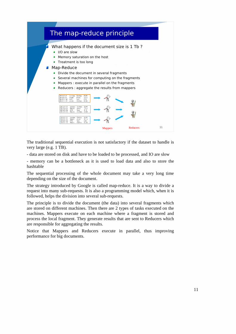
In this figure, we consider several reducers.
The K (words) are distributed between the 2 reduces. For instance, the pairs associated with the Hello word (generated by Map1 and Map2) are both sent to the first reducer. For this word, the reducer receives a pair <Hello, [1,1]> and aggregates the values, generating a pair <Hello, 2>.

24
24
Combiner functions
Reduce data transfer between map and reduceExecuted at the ouput of map
Often the same function as reduce
shuffle&
sort
< Hello, 1> < World, 2> < Bye, 1> < Goodbye, 1> < Man, 1>
< Hello, 1>` < Hadoop, 2> < Goodbye, 2> < Girl, 1>
Reduce
Combiner
Map1
Map2
< Hello, 1> < World, 1> < Bye, 1> < World, 1> < Goodbye, 1> < Man, 1>
< Hello, 1>` < Hadoop, 1> < Goodbye, 1> < Hadoop, 1> < Goodbye, 1> < Girl, 1>
< Man, [1]> < Hadoop, [2]> < Girl, [1]>
< Hello, [1,1]> < World, [2]> < Bye, [1]> < Goodbye, [1,2]>
In some applications, a map may generate a lot of pairs which can be aggregated at the exit of the map, before going through the network. This is a way to decrease the network traffic and therefore to optimize performance.
This is possible in Hadoop thanks to a combiner function which is executed at the exit of each map. The KV are sorted and grouped at the exit of the map, generating a set of <K,{V}> which are handled by the combiner function in the same way as the reduce function, except that this is done on the same node as the map (while the reducer is on a different node).
In the figure, the combiner function is able to aggregate pairs with identical words at the exit of Map1 and Map2.
The interface of a combiner function is the same as the interface of a Reduce function.
Notice that in the WordCount application, we can use the implementation of the reduce function as a combiner function. This is not the case for all applications.

25
25
Main program
public class WordCount { public static void main(String[] args) throws Exception { Configuration conf = new Configuration(); Job job = Job.getInstance(conf, "word count"); job.setJarByClass(WordCount.class); job.setMapperClass(TokenizerMapper.class); job.setCombinerClass(IntSumReducer.class); job.setReducerClass(IntSumReducer.class); job.setOutputKeyClass(Text.class); job.setOutputValueClass(IntWritable.class); FileInputFormat.addInputPath(job, new Path(args[0])); FileOutputFormat.setOutputPath(job, new Path(args[1])); System.exit(job.waitForCompletion(true) ? 0 : 1); }}
Here is the main class of the WordCount application.
It creates a new job which is initialized with :
- the main class
- the mapper class
- the combiner class (the same as the reducer class)
- the reducer class
- the classes for the output (for K and V)
- the path where input data will be found
- the path where output data will be stored
These paths refer to files on the local file system if we run Hadoop standalone (i.e. locally to test a program), or to files in HDFS if we run Hadoop in cluster mode.
26
26
Execution in a cluster
DataNode
Map
HDFS
DataNode DataNode DataNode DataNode DataNode
ReduceMap Map MapReduce
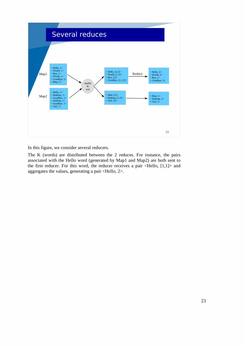
This figure illustrates the execution in a cluster.
HDFS run on all the node with a DataNode daemon.
When running an application, several maps are executed on nodes where blocks are stored. Maps are generating KV which are transmitted to one reduce according to K (blue or red). Each reduce generates a result block which is stored locally in HDFS.

27
27
Evolution from HadoopSpeed: reducing read/write operations
Up to 10 times faster when running on disk
Up to 100 times faster when running in memory
Multiple-languages: Java, Scala or Python
Advance analytics: not only Map-ReduceSQL
Streaming data
Machine Learning
Graph algorithms
Sparks in few words
Spark is an evolution from Hadoop.
One of the main goal was to improve performance, either when used for datasets that fit in memory, or for larger datasets that have to be stored on disk.
Another major improvement is to provide a new programming model (still implementing a map-reduce strategy) for the manipulation of large datasets. This programming model is available in multiple popular languages (Java, Scala or Python).
The Spark environment also provides additional services for
- expressing request in an SQL like syntax
- handling streams of data (arriving continuously)
- applying machine learning algorithms to large datasets
- handling datasets which include graphs

28
28
Programming with Spark (Java)
Initialization
Spark relies on Resilient Distributed Datasets (RDD)Datasets that are partitioned on nodes
Can be operated in parallel
SparkConf conf = new SparkConf().setAppName("WordCount"); JavaSparkContext sc = new JavaSparkContext(conf);
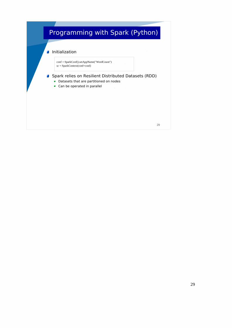
Here is a simple tutorial about programming in Spark. I use Java for the lecture and also for labworks, although I also have a Python version of both.
The first step is to initialize Spark.
You must create a configuration object and then create a spark context object.
This spark context object is then used mainly for accessing (generally from HDFS) the data to be processed.
The Spark programming model relies on Resilient Distributed Datasets or RDD. A RDD is a very large vector of values (any Java object). This vector is partitioned, which means that it is split into fragments (called partitions) that are distributed on different nodes.
This partitioning on nodes allows computations on a RDD to be performed in parallel. For instance, if you want to apply the same operation on each element of one RDD, It can be done in parallel on each node where a partition is stored, each node iterating on the elements it hosts.
29
29
Programming with Spark (Python)
Initialization
Spark relies on Resilient Distributed Datasets (RDD)Datasets that are partitioned on nodes
Can be operated in parallel
conf = SparkConf().setAppName("WordCount") sc = SparkContext(conf=conf)

30
30
Programming with Spark (Java)
RDD created from a Python data
RDD created from an external storage (file)
List<Integer> data = Arrays.asList(1, 2, 3, 4, 5); JavaRDD<Integer> rdd = sc.parallelize(data);
JavaRDD<String> rdd = sc.textFile("data.txt");
You can create a RDD from a Java object (here a list of Integer) with the parallelize() method. Notice that a RDD is typed: here it is a JavaRDD<Integer>
Generally a RDD is large (we are in the Big Data world). It is read from an external storage such as HDFS. In the second example, the textFile() method on the sparkcontext allows to create a RDD from a text file, thus resulting in a JavaRDD<String>. The elements in this RDD are the lines from the text file. This RDD is composed of distributed partitions, each partition corresponding to a block in HDFS.
It is important to note that a RDD is an abstract entity. When you execute textFile(), data are not loaded in memory. It registers that data will be loaded from a text file in the future. The data are effectively loaded when operations are performed on the data.

31
31
Programming with Spark (Python)
RDD created from a Java object
RDD created from an external storage (file)
data = [1, 2, 3, 4, 5] rdd = sc.parallelize(data)
rdd = sc.textFile("data.txt")

32
32
Programming with Spark
Driver program: the main program
Two types of operation on RDDTransformations: create a new RDD from an existing one
e.g. map() passes each RDD element through a given function
Actions: compute a value from a existing RDDe.g. reduce() aggregates all RDD elements using a given function and computes a single value
Transformations are lazily computed when needed to perform an action (optimization)
By default, transformations are cached in memory, but they can be recomputed if they don't fit in memory
The execution of a Spark application first executes the main method in a single process. This process is called the Driver program. Then, the operations on RDDs as distributed, i.e. executed on all the nodes where partitions are located. For instance, if a RDD is initialized with a HDFS file distributed on several nodes (blocks in HDFS), an operation on that RDD will be distributed and executed in parallel on these nodes, where partitions will be loaded from blocks in HDFS.
Two types of operation can be performed on RDD:
- Transformations which create a new RDD from an existing one. An example is a map(f) operation which applies the f function on all elements within the RDD. The resulting RDD is distributed on all the nodes where the existing RDD is.
- Actions which compute a final value from an existing RDD. The result is stored in the Driver program. An example is a reduce(f) operation which aggregates all elements within the existing RDD. The f function takes a pair of elements as parameter and computes the aggregation into one element. The same function f is used to aggregate all the elements into a single value.
Transformations are computed lazily, generally when an action has to be performed. For instance :
rdd=(1,2,3,4)
rdd.map(increment()) // means each element should be incremented
rdd.map(double()) // means each element should be doubled
sum=rdd.reduce(add()) // compute a final value (sum), add() being an additioner // which aggregates 2 elements into one
We don't have to parse the RDD for each map. We can parse the RDD only once and apply both the increment() and double() functions only when the element is considered for aggregating it with another element.
When the result of a transformation is reused for different computations, it is cached in memory. But if memory is lacking, it may be evicted from cache and later recomputed (remember that RDD are immutable, only new RDDs are generated).

33
33
Programming with Spark (Java)
Example with lambda expressionsmap(): apply a function to each element of a RDD
reduce(): apply a function to aggregate all values from a RDDFunction must be associative and commutative for parallelism
Or with Java functions
JavaRDD<String> lines = sc.textFile("data.txt"); JavaRDD<Integer> lineLengths = lines.map(s -> s.length()); int totalLength = lineLengths.reduce((a, b) -> a + b);
class lenFunc implements Function<String, Integer> { public Integer call(String s) { return s.length(); } } JavaRDD<String> lines = sc.textFile("data.txt"); JavaRDD<Integer> lineLengths = lines.map(new lenFunc()); ...
To program functions (f or increment in the previous slide) which can be used in operations (like map() or reduce()), we can use lambda expressions or Java functions. Map and reduce operations were presented in the previous slide.
In this example, lines is a RDD of String, initialized from a data.txt file (may be in HDFS). It contains the lines from the document. The map() operation replaces each line by its length, resulting into a RDD of Integer. The reduce() operation aggregates all the elements from that RDD, using an additioner : (a,b) → a+b
This way of writing a function is a lambda expression.
In a reduce(), the aggregation function must be associative and commutative, which means that the order the elements are aggregated does not matter. For instance, the aggregation of (1,2,3,4) may be performed in these orders:
(1+2) + (3+4) or ((1+2)+3)+4
You provide an aggregation function (commutative and associative) and Spark is responsible for applying it.
In the bottom, you have the equivalent with Java functions. A Java function is a parametric class : Function <param_1, param_2 …, result> where param_i is the type of the ith param, and result the returned type. The class must implement a call() method which is the method invoked when the function is called. Notice in the example that the parameters of the call() method are consistent with those of the class definition.

34
34
Programming with Spark (Python)
Example with lambda expressionsmap(): apply a function to each element of a RDD
reduce(): apply a function to aggregate all values from a RDDFunction must be associative and commutative for parallelism
Or with a function
lines = sc.textFile("data.txt") LineLengths = lines.map(lambda s: len(s)) totalLength = lineLengths.reduce(lambda a, b: a + b)
def lenFunc(s): return len(words)
lines = sc.textFile("data.txt") sc.textFile("file.txt").map(lenFunc) ...

35
35
Programming with Spark (Java)
Execution of operations (transformations/actions) is distributed
Variables in the driver program are serialized and copied on remote hosts (they are not global variables)
Should use special Accumulator/Broadcast variables
int counter = 0; JavaRDD<Integer> rdd = sc.parallelize(data);
// Wrong: Don't do this!! rdd.foreach(x -> counter += x); println("Counter value: " + counter);
You must remember that the executions of transformations and actions are distributed on the nodes of the cluster. This implies that variables in the Driver program (the main method) cannot be used in operations on RDDs. Actually, they are serialized and copied on all the nodes, but their values may be inconsistent.
In the given example, we try to use a variable (counter) in the Driver program to sum values in a RDD (foreach() applies a function on each element of the RDD, but without generating a new RDD).
DON'T DO THAT
Global variables exist in Spark. You should use special variables : Accumulator and Broadcast.

36
36
Programming with Spark (Python)
Execution of operations (transformations/actions) is distributed
Variables in the driver program are serialized and copied on remote hosts (they are not global variables)
Should use special Accumulator/Broadcast variables
counter = 0 rdd = sc.parallelize(data)
# Wrong: Don't do this!! def increment_counter(x): global counter counter += x
rdd.foreach(increment_counter) print("Counter value: ", counter)

37
37
Programming with Spark (Java)
Many operations rely on key-value pairsExample (count the lines)
mapToPairs(): each element of the RDD produces a pair
reduceByKey(): apply a function to aggregate values for each key
JavaRDD<String> lines = sc.textFile("data.txt"); JavaPairRDD<String, Integer> pairs = lines.mapToPair(s -> new Tuple2(s, 1)); JavaPairRDD<String, Integer> counts = pairs.reduceByKey((a, b) -> a + b);
In Spark (as in Hadoop), many operations rely on key-value pairs.
While a RDD of type T is : JavaRDD<T>
A RDD of pairs of types K and V is : JavaPairRDD<K,V>
Such a pair RDD can be generated by a mapToPair(f) operation, f being a function which transforms an element into a pair (an instance of the Tuple2 class in Java).
Another form of reduce operation allows to do what we were doing with Hadoop : sorting/grouping keys and aggregating values for each unique key.
reduceByKey(f) on a pair RDD groups keys and aggregates values with the f function (which should still be associative and commutative)
In the example,
- the mapToPair() operation generates for each element (line) a pair <line,1>. Notice that it returns a JavaPairRDD<String, Integer>
- the reduceByKey() operation groups identical lines and additions all the 1 behind a unique line.
Globally the result gives for each unique line the number of times the line appears in the text file (it counts redundant lines).

38
38
Programming with Spark (Python)
Many operations rely on key-value pairsExample (count the lines)
map(): each element of the RDD produces a pair
reduceByKey(): apply a function to aggregate values for each key
lines = sc.textFile("data.txt") pairs = lines.map(lambda s: (s, 1)) counts = pairs.reduceByKey(lambda a, b: a + b)

39
39
WordCount example (Java)
JavaRDD<String> words = sc.textFile(inputFile).flatMap(s -> Arrays.asList(s.split(" ")).iterator());
JavaPairRDD<String, Integer> counts =
words.mapToPair(w -> new Tuple2<String, Integer>(w,1)).reduceByKey((a,b) -> a + b);
Here is the implementation of the WordCount example that we saw in Hadoop.
- the split() method returns a String[]
- asList() returns a List<String>
- like map(f), flatMap(f) applies the f function on each element of the RDD. The difference is that map() generates for each element one element in the result RDD, while flatMap() may generate 0 or n elements. The function f in flatMap(f) should return an iterator used by Spark to insert the generated elements in the result RDD. In this example, the function in flatMap() splits each line into words and returns an iterator on the list of words. The flatMap() returns a JavaRDD<String> includeing all the words.
- mapToPair() generates for each word w a pair <w, 1>
- reduceByKey() groups words and additions all the 1 behind each unique word
JavaRDD<String> data = sc.textFile(inputFile);
// returns ("toto titi tutu", "tata titi toto", "tata toto tutu")
JavaRDD<String> words = data.flatMap(s -> Arrays.asList(s.split(" ")).iterator());
// returns ("toto", "titi", "tutu", "tata", "titi", "toto", "tata", "toto", "tutu")
JavaPairRDD<String, Integer> pairs =
words.mapToPair(w -> new Tuple2<String, Integer>(w,1));
// returns (("toto",1), ("titi",1), ("tutu",1), ("tata",1), ("titi",1), ("toto",1), ("tata",1), ("toto",1), ("tutu",1))
JavaPairRDD<String, Integer> counts = pairs.reduceByKey((c1,c2) -> c1 + c2);
// group words (("toto",{1,1,1}), ("titi",{1,1}), ("tutu",{1,1}), ("tata",{1,1}))
// and then addition (("toto",3), ("titi",2), ("tutu",2), ("tata",2))

40
40
WordCount example (Python)
words = sc.textFile(inputFile).flatMap(lambda line : line.split(" "))
counts = words.map(lambda w : (w, 1)).reduceByKey(lambda a, b: a + b)

41
41
Many APIs
42
42
Using Spark (Java)
Install Sparktar xzf spark-2.2.0-bin-hadoop2.7.tgz
Define environment variablesexport SPARK_HOME=<path>/spark-2.2.0-bin-hadoop2.7
export PATH=$PATH:$SPARK_HOME/bin:$SPARK_HOME/sbin
Development with eclipseCreate a Java Project
Add jars in the build path• $SPARK_HOME/jars/spark-core_2.11-2.2.0.jar
• $SPARK_HOME/jars/scala-library-2.11.8.jar
• $SPARK_HOME/jars/hadoop-common-2.7.3.jar
• Could include all jars, but not very clean
Your application should be packaged in a jar
Launch the applicationspark-submit --class <classname> --master <url-master> <jarfile>
Centralized: <url-master> = local or local[n]
Cluster: <url-master> = url to access the cluster's master
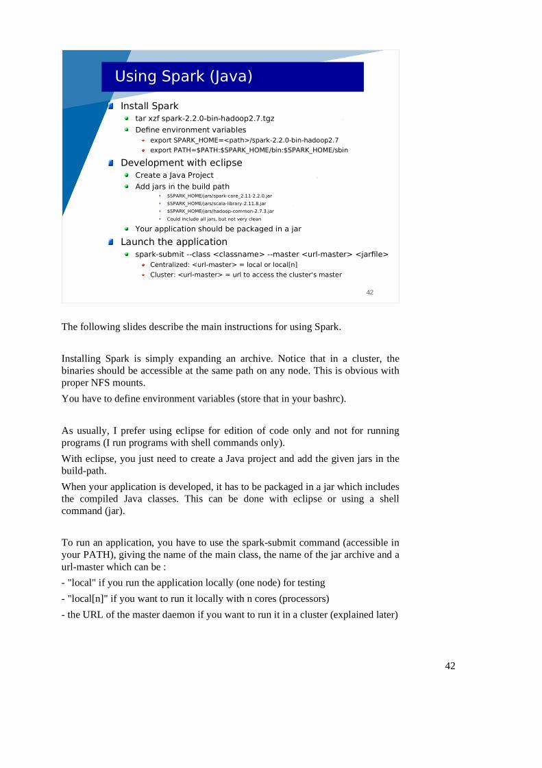
The following slides describe the main instructions for using Spark.
Installing Spark is simply expanding an archive. Notice that in a cluster, the binaries should be accessible at the same path on any node. This is obvious with proper NFS mounts.
You have to define environment variables (store that in your bashrc).
As usually, I prefer using eclipse for edition of code only and not for running programs (I run programs with shell commands only).
With eclipse, you just need to create a Java project and add the given jars in the build-path.
When your application is developed, it has to be packaged in a jar which includes the compiled Java classes. This can be done with eclipse or using a shell command (jar).
To run an application, you have to use the spark-submit command (accessible in your PATH), giving the name of the main class, the name of the jar archive and a url-master which can be :
- "local" if you run the application locally (one node) for testing
- "local[n]" if you want to run it locally with n cores (processors)
- the URL of the master daemon if you want to run it in a cluster (explained later)

43
43
Using Spark (Python)
Install Python3The default Python should refer to Python3
Install Sparktar xzf spark-2.2.0-bin-hadoop2.7.tgz
Define environment variablesexport SPARK_HOME=<path>/spark-2.2.0-bin-hadoop2.7
export PATH=$PATH:$SPARK_HOME/bin:$SPARK_HOME/sbin
Development with eclipseGo to the Help/MarketPlace and install PyDev
Go to Windows/Preferences … Python InterpreterLibraries/New Zip
• add <SPARK_HOME>/python/lib/py4j-0.10.7-src.zip
• add <SPARK_HOME>/python/lib/pyspark.zip
Environment• add SPARK_HOME = <SPARK_HOME>

44
44
Using Spark (Python)
Development with eclipseCreate a PyDev Project
Develop your modules
Launch the applicationspark-submit --master <url-master> <python-file>
Centralized: <url-master> = local or local[n]
Cluster: <url-master> = url to access the cluster's master

45
45
Cluster mode
Starting the masterstart-master.sh
You can check its state and see its URL at http://master:8080
Starting slavesstart-slave.sh -c 1 <url master>
// -c 1 to use only one core
FilesIf not running on top of HDFS, you have to replicate your files on the slaves
Else you program should refer to the input file in HDFS with a URL
To deploy a cluster, you have to launch :
- start-master.sh on the master node to start the master daemon
You can check its state with a web console (and also copy the URL of the master, spark://masternode:7077)
- start-slaves.sh on the master node to start the worker daemons on the slave nodes (assuming that you have configured a "slaves" file describing the nodes where workers should be started)
Alternatively, you can start slaves (by hand) on each node with start-slave.sh giving as parameter the URL of the master.

46
46
Conclusion
Spark is just the beginning
You should have a look atSpark streaming
Spark SQL
ML Lib
GraphX
...