Introduction to Automata Theory - Notesvillagenotesvillage.com/upload/MODULE II.pdfR 703 Theory of Computation 2.5 Deterministic Finite Automata can be defined as M=(Q,Σ,δ,q0,F)

R 703 Theory of Computation 2.1

Introduction to Automata TheoryAutomata theory is basically about the study of different mechanisms for generation and

recognition of languages. Automata theory is basically for the study of different types of grammars and automata. A grammar is a mechanism for the generation of sentences in a language. Automata is a mechanism for recognition of languages. Automata theory is mainly for the study of different kinds of automata as language recognizers and their relationship with grammars.

In theoretical computer science, automata theory is the study of abstract machines and problems they are able to solve. Automata theory is closely related to formal language theory as the automata are often classified by the class of formal languages they are able to recognize.

An automaton is a mathematical model for a finite state machine (FSM). A FSM is a machine that, given an input of symbols, "jumps" through a series of states according to a transition function (which can be expressed as a table). In the common "Mealy" variety of FSMs, this transition function tells the automaton which state to go to next given a current state and a current symbol.

The input is read symbol by symbol, until it is consumed completely (think of it as a tape with a word written on it, that is read by a reading head of the automaton; the head moves forward over the tape, reading one symbol at a time). Once the input is depleted, the automaton is said to have stopped.

Depending on the state in which the automaton stops, it's said that the automaton either accepts or rejects the input. If it landed in an accept state, then the automaton accepts the word. If, on the other hand, it lands on a reject state, the word is rejected. The set of all the words accepted by an automaton is called the language accepted by the automaton.

Automata play a major role in compiler design and parsing.

Finite Automata is the simplest one of different classes of automata. Mainly there are 3 variants of finite automata. They are:Deterministic Finite AutomataNon-deterministic Finite AutomataNon-deterministic Finite Automata with Є-transition.

Here we define the acceptability of strings by finite automata.

Computer Science & Engineering. Dept. SJCET, Palai

http://en.wikipedia.org/wiki/Theoretical_computer_science

http://en.wikipedia.org/wiki/Formal_language

http://en.wikipedia.org/wiki/Mealy_machine

http://en.wikipedia.org/wiki/Transition_function

http://en.wikipedia.org/wiki/Finite_state_machine


http://en.wikipedia.org/wiki/Automata

http://en.wikipedia.org/wiki/Formal_language_theory

http://en.wikipedia.org/wiki/Abstract_machine


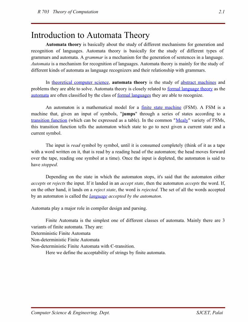
Description of AutomatonAn automaton can be defined in an abstract way by the following figure.

i) Input: - At each of the discrete instants of time t1,t2,…..input values I1,I2……… each of

which can take a finite number of fixed values from the input alphabet Σ, are applied to the input side of the model.

ii) Output : - O1,O2….are the outputs of the model, each of which can take finite numbers of fixed values from an output O.

iii) States : - At any instant of time the automaton can be in one of the states q1,q2…..qniv) State relation : - The next state of an automaton at any instant of time is determined by

the present state and the present input. ie, by the transition function.v) Output relation : - Output is related to either state only or both the input and the state. It

should be noted that at any instant of time the automaton is in some state. On 'reading' an input symbol, the automaton moves to a next state which is given by the state relation.

An automaton in which the output depends only on the input is called an automaton without a memory. An automaton in which the output depends on the states also is called automaton with a finite memory. An automaton in which the output depends only on the states of the machine is called a Moore Machine. An automaton in which the output depends on the state and the input at any instant of time is called a Mealy machine.

Definition of a finite automatonBasic model of finite automata consists of :

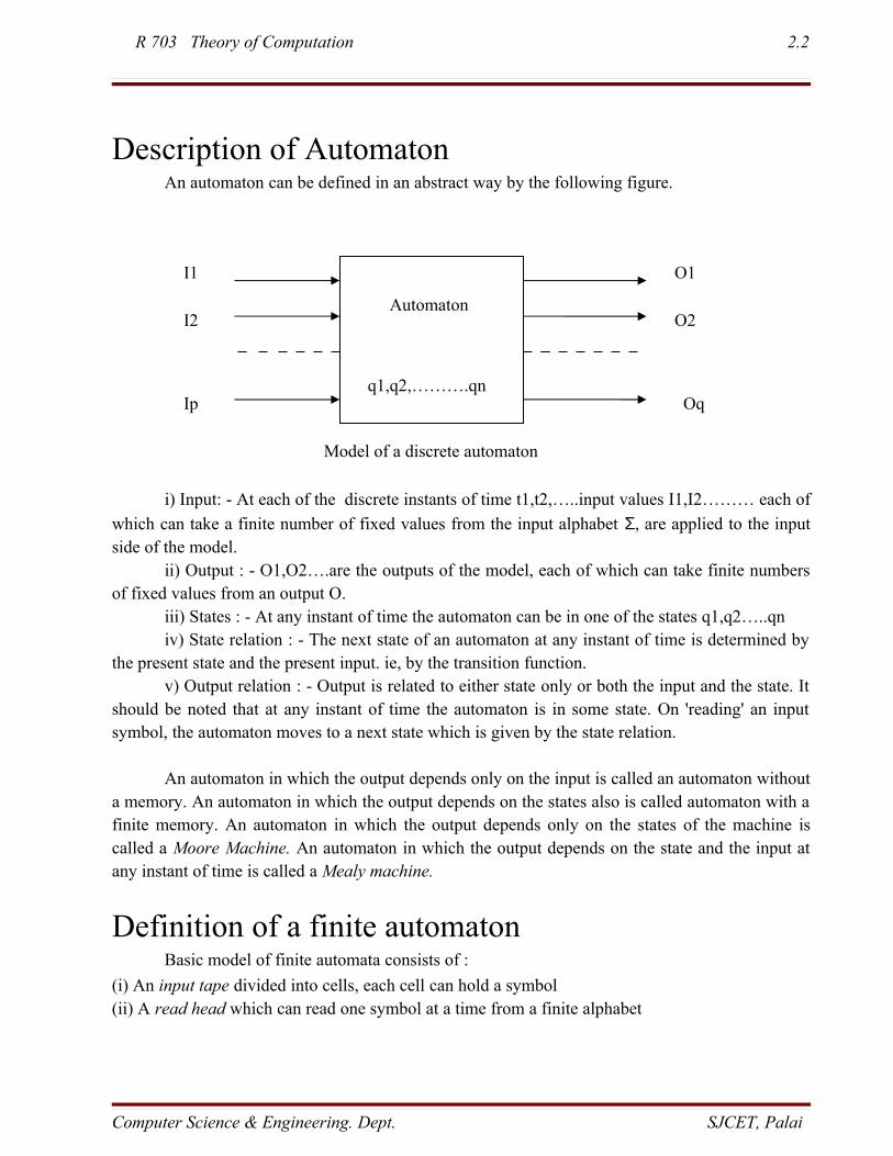
(i) An input tape divided into cells, each cell can hold a symbol(ii) A read head which can read one symbol at a time from a finite alphabet


O1

O2

Oq

I1

I2

Ip

Automaton

q1,q2,……….qn

Model of a discrete automaton


(iii) A finite control which works within a finite set of states. At each step, it changes its state depending on the current state and input read. Its change of state is specified by a transition function. It accepts the input if it is in a set of accepting states.

a) Finite Automata – Formal DefinitionA finite automaton can be represented by a 5-tuple (Q,Σ,δ,q0,F) where

Q – finite set of internal states

Σ - finite set of symbols called input alphabetδ – transition function q0 Є Q – start state or initial state

F ⊆ Q – set of accepting states or final statesTransition function describes the change of states during the transition. This mapping is

usually represented by Transition diagram or Transition table.

Transition diagrams and Transition SystemsA transition graph or a transition system is a finite directed labeled graph in which each

vertex (node) represents a state and the directed edges indicate the transition of a state and the edges are labelled with input. A transition graph contains:(i) A finite set of states, one of which are designated as start state and some of which are designated as final states.

(ii) An alphabet Σ of possible input letters from which input strings are formed.(iii) A finite set of transitions that show, how to go from some states to some other states.

So a transition system is a 5-tuple (Q,Σ,δ,q0,F)


Finite Control

Input Tape

Read Head

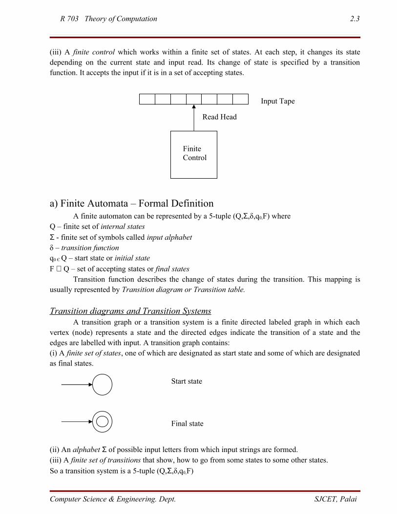
Start state

Final state


If δ(qi,a)=qj, there is an edge labeled by 'a' from qi to qj . A transition system accepts a string

'w' in Σ* if 1) there exists a path which originates from some initial state, goes along the arrows, and

terminates at some final state.2) the path value obtained by concatenation of all edge-labels of the path is equal to 'w'.

Transition Table

The description of the automation can be given in the form of transition table also, in which we tabulate the details of the transitions defined be the automaton from one state to another.

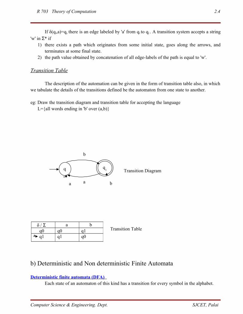
eg: Draw the transition diagram and transition table for accepting the language L={all words ending in 'b' over (a,b)}

b) Deterministic and Non deterministic Finite Automata

Deterministic fin ite automata (DFA) Each state of an automaton of this kind has a transition for every symbol in the alphabet.


q

0

q1

a

b

a b

Transition Diagram

δ / Σ a b q0 q0 q1* q1 q1 q0

Transition Table

http://en.wikipedia.org/wiki/Deterministic_finite_state_machine


Deterministic Finite Automata can be defined as M=(Q,Σ,δ,q0,F) where Q is the set of states

Σ is the input symbols

δ is the transition function Q x Σ Qq0 is the start stateF is the final state

Nondeterministic finite automata (NFA)States of an automaton of this kind may or may not have a transition for each symbol in the

alphabet, or can even have multiple transitions for a symbol. The automaton accepts a word if there exists at least one path from q0 to a state in F labeled with the input word. If a transition is undefined, so that the automaton does not know how to keep on reading the input, the word is rejected. NFA is equivalent to the DFA.

Non-Deterministic Finite Automata also can be defined as M=(Q,Σ,δ,q0,F) where Q is the set of states

Σ is the input symbols

δ is the transition function Q x Σ 2Q

q0 is the start stateF is the final state

Nondeterministic finite automata, with ε transitions (FND-ε or ε-NFA) Besides of being able to jump to more (or none) states with any symbol, these can jump on no symbol at all. That is, if a state has transitions labeled with ε, then the NFA can be in any of the states reached by the ε-transitions, directly or through other states with ε-transitions. The set of states that can be reached by this method from a state q, is called the ε-closure of q.

Moore machi ne The FSM uses only entry actions, i.e. output depends only on the state. The advantage of the Moore model is a simplification of the behaviour. The example in figure 1 shows a Moore FSM of an elevator door. The state machine recognizes two commands: "command_open" and "command_close" which trigger state changes. The entry action (E:) in state "Opening" starts a motor opening the door, the entry action in state "Closing" starts a motor in the other direction closing the door. States "Opened" and "Closed" don't perform any actions. They signal to the outside world (e.g. to other state machines) the situation: "door is open" or "door is closed".


http://en.wikipedia.org/wiki/Moore_machine

http://en.wikipedia.org/wiki/Nondeterministic_finite_state_machine

http://en.wikipedia.org/wiki/Nondeterministic_finite_state_machine


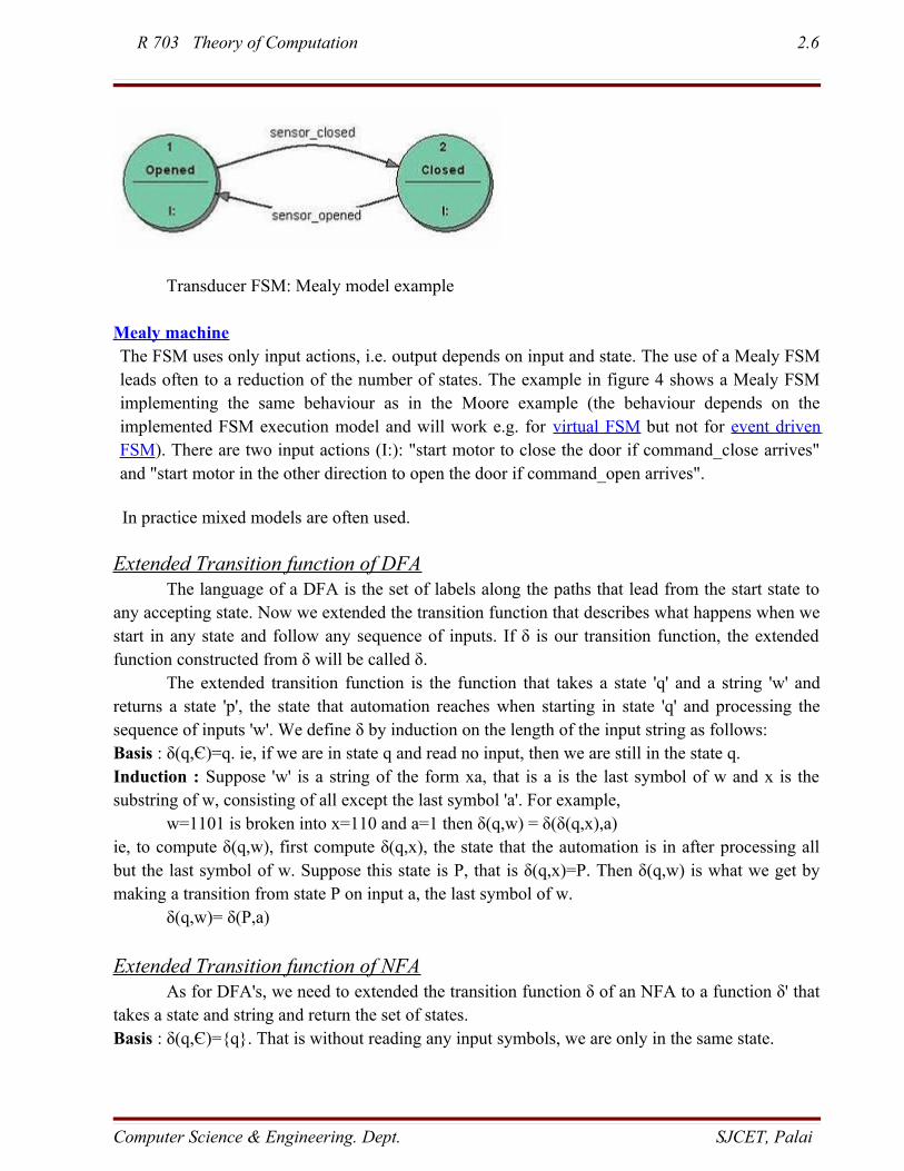
Transducer FSM: Mealy model example

Mealy machine The FSM uses only input actions, i.e. output depends on input and state. The use of a Mealy FSM leads often to a reduction of the number of states. The example in figure 4 shows a Mealy FSM implementing the same behaviour as in the Moore example (the behaviour depends on the implemented FSM execution model and will work e.g. for virtual FSM but not for event driven FSM). There are two input actions (I:): "start motor to close the door if command_close arrives" and "start motor in the other direction to open the door if command_open arrives".

In practice mixed models are often used.

Extended Transition function of DFAThe language of a DFA is the set of labels along the paths that lead from the start state to

any accepting state. Now we extended the transition function that describes what happens when we start in any state and follow any sequence of inputs. If δ is our transition function, the extended function constructed from δ will be called δ.

The extended transition function is the function that takes a state 'q' and a string 'w' and returns a state 'p', the state that automation reaches when starting in state 'q' and processing the sequence of inputs 'w'. We define δ by induction on the length of the input string as follows:Basis : δ(q,Є)=q. ie, if we are in state q and read no input, then we are still in the state q.Induction : Suppose 'w' is a string of the form xa, that is a is the last symbol of w and x is the substring of w, consisting of all except the last symbol 'a'. For example,

w=1101 is broken into x=110 and a=1 then δ(q,w) = δ(δ(q,x),a)ie, to compute δ(q,w), first compute δ(q,x), the state that the automation is in after processing all but the last symbol of w. Suppose this state is P, that is δ(q,x)=P. Then δ(q,w) is what we get by making a transition from state P on input a, the last symbol of w.

δ(q,w)= δ(P,a)

Extended Transition function of NFAAs for DFA's, we need to extended the transition function δ of an NFA to a function δ' that

takes a state and string and return the set of states. Basis : δ(q,Є)={q}. That is without reading any input symbols, we are only in the same state.


http://en.wikipedia.org/wiki/Event_driven_finite_state_machine

http://en.wikipedia.org/wiki/Event_driven_finite_state_machine

http://en.wikipedia.org/wiki/Virtual_finite_state_machine

http://en.wikipedia.org/wiki/Mealy_machine

http://en.wikipedia.org/wiki/Image:Fsm_mealy_model_door_control.jpg


Induction : Suppose w is of the form w=xa, where a is the last symbol and x is the substring containing rest of w. Let us suppose that

δ(q,x)={p1,p2…..pk}Let U δ(pi,a)={r1,r2……….rm} thenδ(q,w)={r1,r2……..rm}. Less formally, we compute δ(q,w) by first computing δ(q,x), and by then following any transition from any of these states that is labeled a.

Language acceptability by Finite AutomataSuppose a1,a2,a3………….an is a sequence of input symbols, q0,q1,q2…….qn are set of

states where q0 is start state and qn is final state and transition function processed asδ(q0,a1)=q1δ(q1,a2)=q2δ(q2,a3)=q3.......δ(qn-1,an)=qn

Input a1,a2,a3……..an is said to be 'accepted ' since qn is a member of the final state, and if not then it is 'rejected'.

Language accepted by DFA 'M' written asL(M)={w/ δ(q0,w)=qf for some qf in F}

Examples of DFA

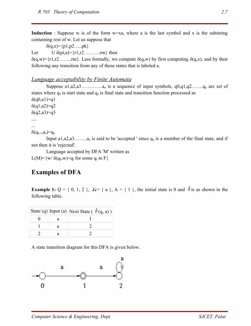
Example 1: Q = { 0, 1, 2 }, = { a }, A = { 1 }, the initial state is 0 and is as shown in the following table.

A state transition diagram for this DFA is given below.


State (q) Input (a) Next State ( (q, a) )

0 a 1

1 a 2

2 a 2


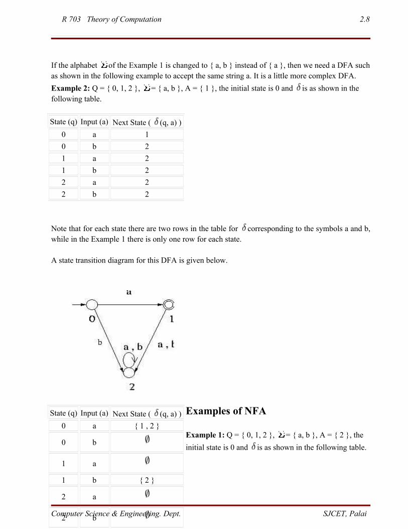
If the alphabet of the Example 1 is changed to { a, b } instead of { a }, then we need a DFA such as shown in the following example to accept the same string a. It is a little more complex DFA.

Example 2: Q = { 0, 1, 2 }, = { a, b }, A = { 1 }, the initial state is 0 and is as shown in the following table.

Note that for each state there are two rows in the table for corresponding to the symbols a and b, while in the Example 1 there is only one row for each state.

A state transition diagram for this DFA is given below.

Examples of NFA

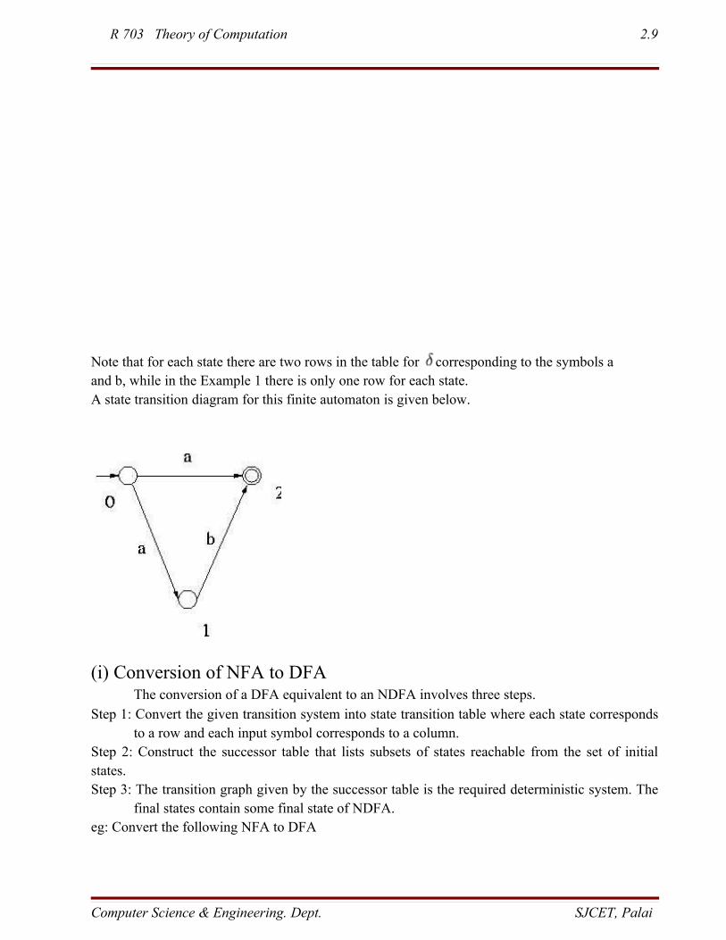
Example 1: Q = { 0, 1, 2 }, = { a, b }, A = { 2 }, the

initial state is 0 and is as shown in the following table.



0 a 1

0 b 2

1 a 2

1 b 2

2 a 2

2 b 2


0 a { 1 , 2 }

0 b

1 a

1 b { 2 }

2 a

2 b


Note that for each state there are two rows in the table for corresponding to the symbols aand b, while in the Example 1 there is only one row for each state. A state transition diagram for this finite automaton is given below.

(i) Conversion of NFA to DFAThe conversion of a DFA equivalent to an NDFA involves three steps.

Step 1: Convert the given transition system into state transition table where each state corresponds to a row and each input symbol corresponds to a column.

Step 2: Construct the successor table that lists subsets of states reachable from the set of initial states.Step 3: The transition graph given by the successor table is the required deterministic system. The

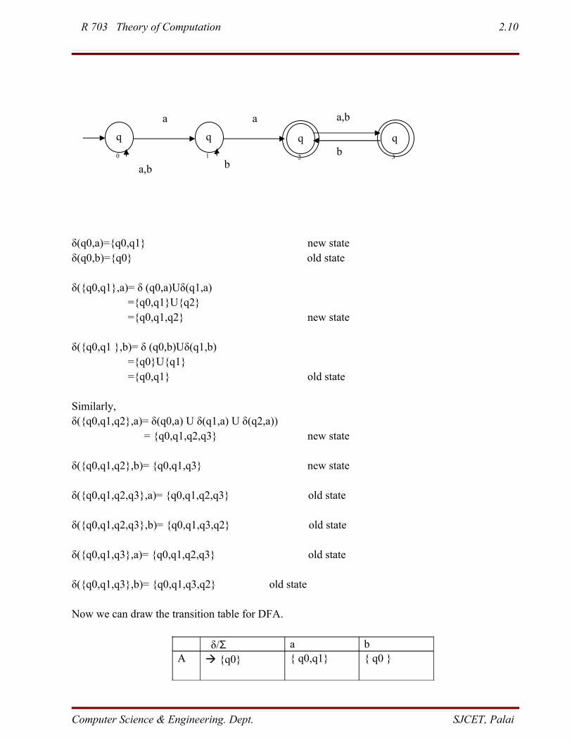
final states contain some final state of NDFA.eg: Convert the following NFA to DFA



δ(q0,a)={q0,q1} new stateδ(q0,b)={q0} old state

δ({q0,q1},a)= δ (q0,a)Uδ(q1,a) ={q0,q1}U{q2} ={q0,q1,q2} new state

δ({q0,q1 },b)= δ (q0,b)Uδ(q1,b) ={q0}U{q1} ={q0,q1} old state

Similarly,δ({q0,q1,q2},a)= δ(q0,a) U δ(q1,a) U δ(q2,a))

= {q0,q1,q2,q3} new state

δ({q0,q1,q2},b)= {q0,q1,q3} new state

δ({q0,q1,q2,q3},a)= {q0,q1,q2,q3} old state

δ({q0,q1,q2,q3},b)= {q0,q1,q3,q2} old state

δ({q0,q1,q3},a)= {q0,q1,q2,q3} old state

δ({q0,q1,q3},b)= {q0,q1,q3,q2} old state

Now we can draw the transition table for DFA.

δ/Σ a bA {q0} { q0,q1} { q0 }


q

0

q

1

q

2

aa

ba,b

q

3

a,b

b


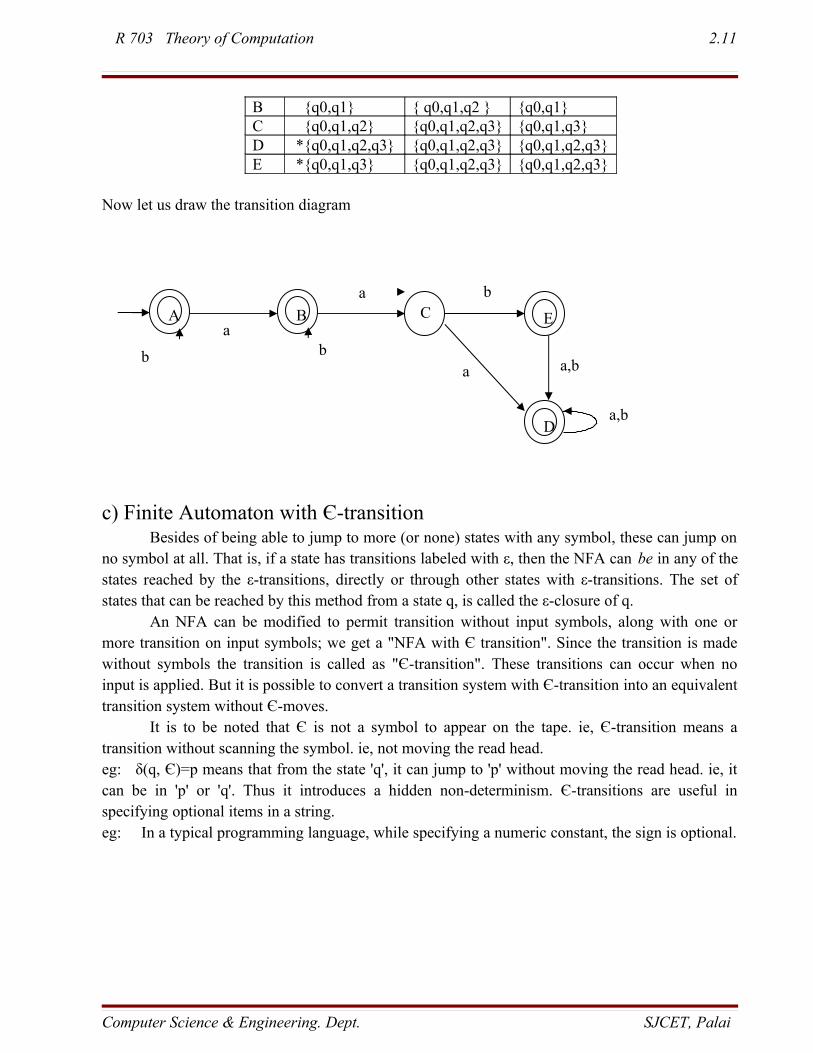
B {q0,q1} { q0,q1,q2 } {q0,q1}C {q0,q1,q2} {q0,q1,q2,q3} {q0,q1,q3}D *{q0,q1,q2,q3} {q0,q1,q2,q3} {q0,q1,q2,q3}E *{q0,q1,q3} {q0,q1,q2,q3} {q0,q1,q2,q3}

Now let us draw the transition diagram

c) Finite Automaton with Є-transitionBesides of being able to jump to more (or none) states with any symbol, these can jump on

no symbol at all. That is, if a state has transitions labeled with ε, then the NFA can be in any of the states reached by the ε-transitions, directly or through other states with ε-transitions. The set of states that can be reached by this method from a state q, is called the ε-closure of q.

An NFA can be modified to permit transition without input symbols, along with one or more transition on input symbols; we get a "NFA with Є transition". Since the transition is made without symbols the transition is called as "Є-transition". These transitions can occur when no input is applied. But it is possible to convert a transition system with Є-transition into an equivalent transition system without Є-moves.

It is to be noted that Є is not a symbol to appear on the tape. ie, Є-transition means a transition without scanning the symbol. ie, not moving the read head.eg: δ(q, Є)=p means that from the state 'q', it can jump to 'p' without moving the read head. ie, it can be in 'p' or 'q'. Thus it introduces a hidden non-determinism. Є-transitions are useful in specifying optional items in a string.eg: In a typical programming language, while specifying a numeric constant, the sign is optional.


Ca

abb

BAa

E

b

D

a,b

a,b


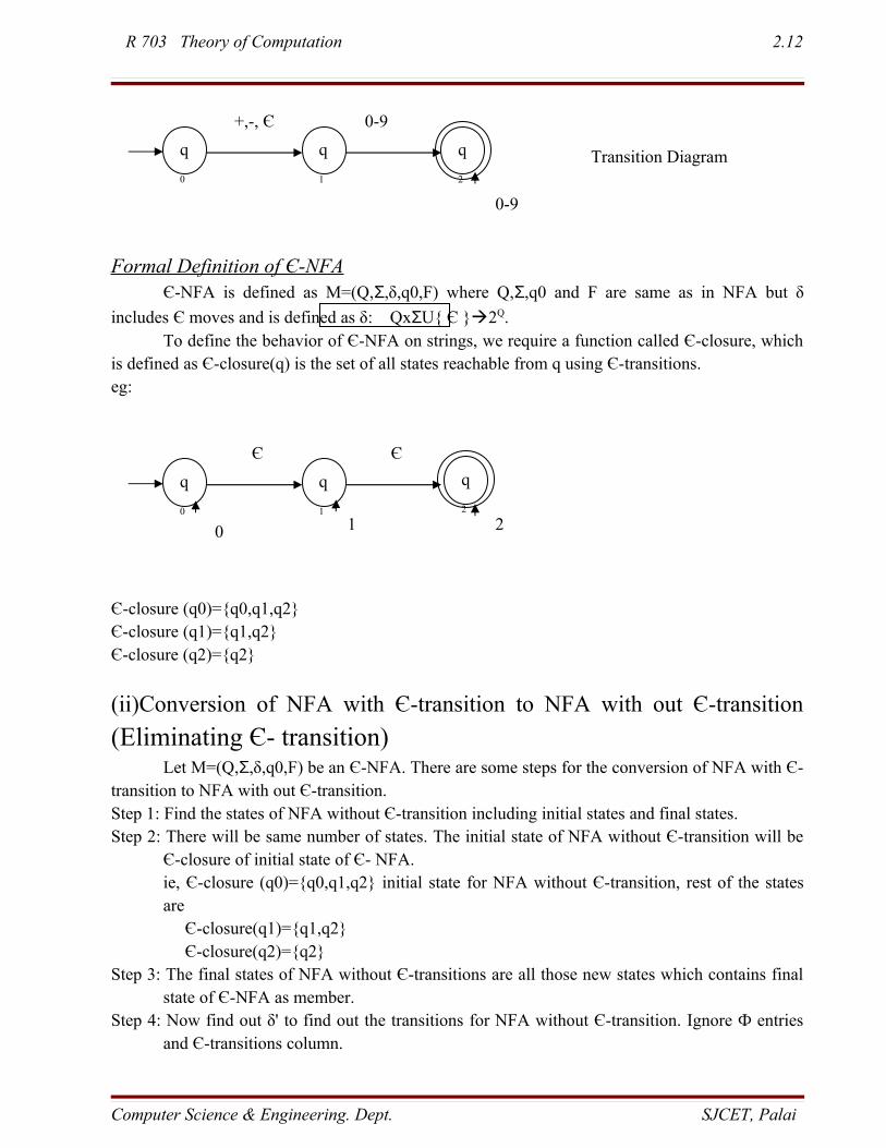
Formal Definition of Є-NFAЄ-NFA is defined as M=(Q,Σ,δ,q0,F) where Q,Σ,q0 and F are same as in NFA but δ

includes Є moves and is defined as δ: QxΣU{ Є }2Q.To define the behavior of Є-NFA on strings, we require a function called Є-closure, which

is defined as Є-closure(q) is the set of all states reachable from q using Є-transitions.eg:

Є-closure (q0)={q0,q1,q2}Є-closure (q1)={q1,q2}Є-closure (q2)={q2}

(ii)Conversion of NFA with Є-transition to NFA with out Є-transition

(Eliminating Є- transition)Let M=(Q,Σ,δ,q0,F) be an Є-NFA. There are some steps for the conversion of NFA with Є-

transition to NFA with out Є-transition. Step 1: Find the states of NFA without Є-transition including initial states and final states.Step 2: There will be same number of states. The initial state of NFA without Є-transition will be

Є-closure of initial state of Є- NFA.ie, Є-closure (q0)={q0,q1,q2} initial state for NFA without Є-transition, rest of the states are Є-closure(q1)={q1,q2} Є-closure(q2)={q2}

Step 3: The final states of NFA without Є-transitions are all those new states which contains final state of Є-NFA as member.

Step 4: Now find out δ' to find out the transitions for NFA without Є-transition. Ignore Ф entries and Є-transitions column.


q

0

q

1

Transition Diagramq

2

+,-, Є 0-9

0-9

q

0

q

1

q

2

Є

2

Є

010


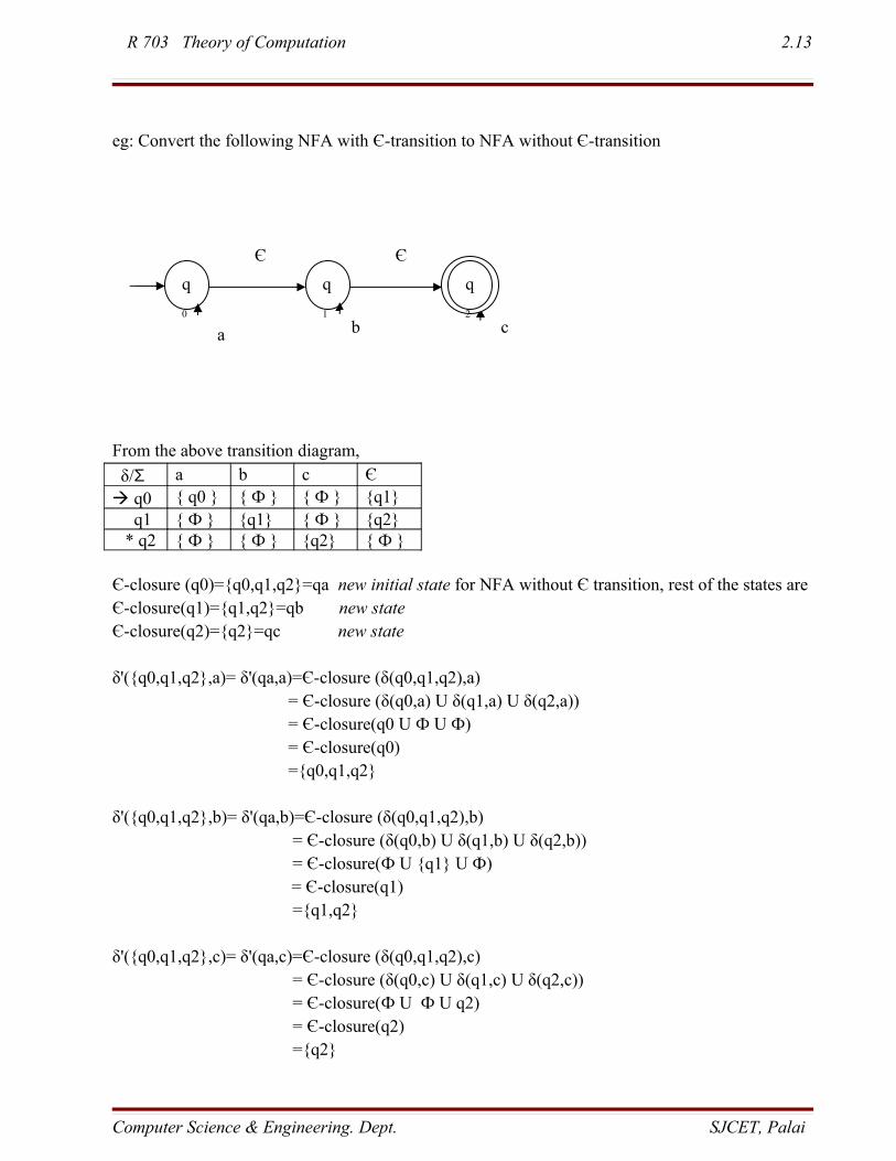
eg: Convert the following NFA with Є-transition to NFA without Є-transition

From the above transition diagram,

δ/Σ a b c Є q0 { q0 } { Ф } { Ф } {q1} q1 { Ф } {q1} { Ф } {q2} * q2 { Ф } { Ф } {q2} { Ф }

Є-closure (q0)={q0,q1,q2}=qa new initial state for NFA without Є transition, rest of the states areЄ-closure(q1)={q1,q2}=qb new stateЄ-closure(q2)={q2}=qc new state

δ'({q0,q1,q2},a)= δ'(qa,a)=Є-closure (δ(q0,q1,q2),a)= Є-closure (δ(q0,a) U δ(q1,a) U δ(q2,a))

= Є-closure(q0 U Ф U Ф) = Є-closure(q0)

={q0,q1,q2}

δ'({q0,q1,q2},b)= δ'(qa,b)=Є-closure (δ(q0,q1,q2),b) = Є-closure (δ(q0,b) U δ(q1,b) U δ(q2,b)) = Є-closure(Ф U {q1} U Ф)

= Є-closure(q1) ={q1,q2}

δ'({q0,q1,q2},c)= δ'(qa,c)=Є-closure (δ(q0,q1,q2),c) = Є-closure (δ(q0,c) U δ(q1,c) U δ(q2,c)) = Є-closure(Ф U Ф U q2) = Є-closure(q2) ={q2}


q

0

q

1

Є

c

Є

ba

q

2


δ'({q1,q2},a)= δ'(qb,a)=Є-closure (δ(q1,q2),a)= Є-closure (δ(q1,a) U δ(q2,a))

= Є-closure(Ф U Ф)= Є-closure(Ф)= Ф

δ'({q1,q2},b)= δ'(qb,b)=Є-closure (δ(q1,q2),b)= Є-closure (δ(q1,b) U δ(q2,b))= Є-closure(q1 U Ф)= Є-closure(q1)= {q1,q2}

δ'({q1,q2},c)= δ'(qb,c)=Є-closure (δ(q1,q2),c)= Є-closure (δ(q1,c) U δ(q2,c))= Є-closure(Ф U q2)= Є-closure(q2)= {q2}

δ'({q2},a)= δ'(qc,a)=Є-closure (δ(q2),a) = Ф

δ'({q2},b)= δ'(qc,b)=Є-closure (δ(q2),b) = Ф

δ'({q2},c)= δ'(qc,c)=Є-closure (δ(q2),c) = Є-closure(q2)

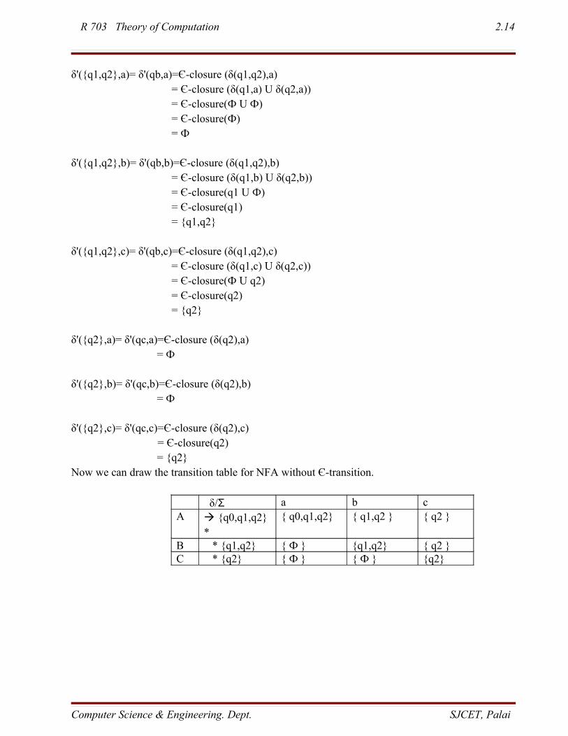
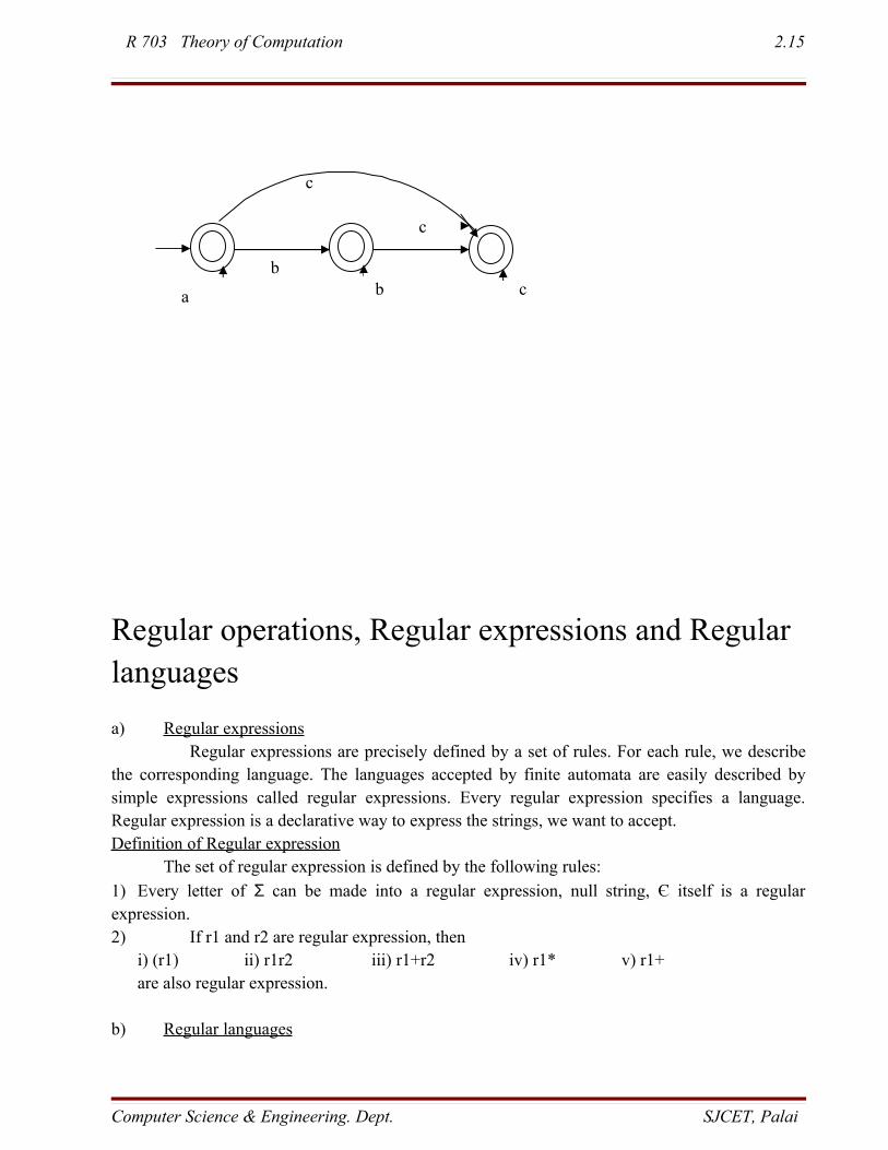
= {q2} Now we can draw the transition table for NFA without Є-transition.

δ/Σ a b cA {q0,q1,q2}

*

{ q0,q1,q2} { q1,q2 } { q2 }

B * {q1,q2} { Ф } {q1,q2} { q2 }C * {q2} { Ф } { Ф } {q2}



Regular operations, Regular expressions and Regular languages

a) Regular expressions Regular expressions are precisely defined by a set of rules. For each rule, we describe

the corresponding language. The languages accepted by finite automata are easily described by simple expressions called regular expressions. Every regular expression specifies a language. Regular expression is a declarative way to express the strings, we want to accept.Definition of Regular expression

The set of regular expression is defined by the following rules:

1) Every letter of Σ can be made into a regular expression, null string, Є itself is a regular expression.2) If r1 and r2 are regular expression, then

i) (r1) ii) r1r2 iii) r1+r2 iv) r1* v) r1+ are also regular expression.

b) Regular languages


c

c

c

ba

b


Regular languages are those that can be generated by applying certain standard operations like union, concatenation and closure, a finite number of times. They can be recognized by finite automata.

Let Σ be an alphabet. The regular expressions over Σ and the sets that they denote are defined recursively as follows.

1) Φ is a regular expression and denotes the empty set.

2) ε is a regular expression and denotes the set {ε}.

3) For each 'a' in Σ, a is a regular expression and denotes the set {a}.

These are known as simple regular languages. Regular language over an alphabet Σ is one that can be obtained from these basic (simple) languages using the operations of union, concatenation and closure, a finite number of times.

c) Regular operations Mainly there are 3 operations on regular expressions. They are union, concatenation, and

kleene closure operation.

If L1 and L2 are any elements of set R of regular languages over ∑ and r1 and r2 are the corresponding regular expressions,i) Union – (L1 U L2) corresponding regular expression is (r1+r2)ii) Concatenation – (L1.L2) corresponding regular expression is (r1. r2)iii) Kleene closure – (L1*) corresponding regular expression is (r1)*

Algebra of Regular Expression

Regular expressions satisfy the following algebraic identities. These identities help us in simplifying regular expressions.(1) Identity Law

∈.R=R.∈=R

Φ+R=R+Φ=R(2) Idempotent Law

R+R=R(R*)=R*

(3) Distributive LawA.(B+C)=A.B+A.C

(4) Associative LawA.(B.C)=(A.B).CA+(B+C)=(A+B)+C

(5) Annihilation

Φ.R=R.Φ=Φ



Example 1: It is easy to see that the RE (0+1)*(0+11) represents the language of all strings over {0,1} which are either ended with 0 or 11.

Example 2: Consider the language of strings over {0,1} containing two or more 1's.

Solution : There must be at least two 1's in the RE somewhere and what comes before, between, and after is completely arbitrary. Hence we can write the RE as (0+1)*1(0+1)*1(0+1)*. But following two REs also represent the same language, each ensuring presence of least two 1's somewhere in the string

i) 0*10*1(0+1)*

ii) (0+1)*10*10*

iii) Regular Expression to Finite state Automata :

Lemma : If L(r) is a language described by the RE r, then it is regular i.e. there is a FA such that L(M) L(r).

Proof : To prove the lemma, we apply structured index on the expression r. First, we show how to

construct FA for the basis elements: , and for any . Then we show how to combine these Finite Automata into Complex Automata that accept the Union, Concatenation, Kleen Closure of the languages accepted by the original smaller automata.

Use of NFAs is helpful in the case i.e. we construct NFAs for every REs which are represented by transition diagram only.

Basis :

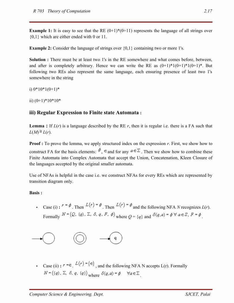
• Case (i) : . Then . Then and the following NFA N recognizes L(r).

Formally where Q = {q} and .

• Case (ii) : . , and the following NFA N accepts L(r). Formally

where .



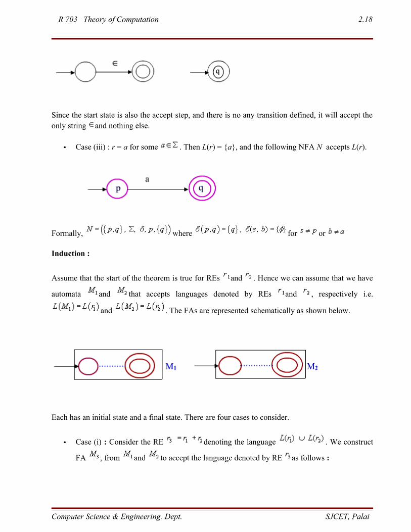
Since the start state is also the accept step, and there is no any transition defined, it will accept the only string and nothing else.

• Case (iii) : r = a for some . Then L(r) = {a}, and the following NFA N accepts L(r).

Formally, where for or

Induction :

Assume that the start of the theorem is true for REs and . Hence we can assume that we have

automata and that accepts languages denoted by REs and , respectively i.e.

and . The FAs are represented schematically as shown below.

Each has an initial state and a final state. There are four cases to consider.

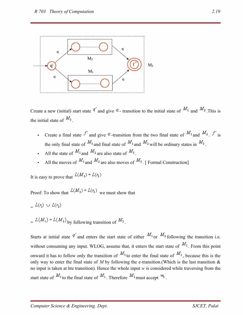
• Case (i) : Consider the RE denoting the language . We construct

FA , from and to accept the language denoted by RE as follows :



Create a new (initial) start state and give - transition to the initial state of and .This is

the initial state of .

• Create a final state and give -transition from the two final state of and . is

the only final state of and final state of and will be ordinary states in .

• All the state of and are also state of .

• All the moves of and are also moves of . [ Formal Construction]

It is easy to prove that

Proof: To show that we must show that

=

= by following transition of .

Starts at initial state and enters the start state of either or following the transition i.e.

without consuming any input. WLOG, assume that, it enters the start state of . From this point

onward it has to follow only the transition of to enter the final state of , because this is the only way to enter the final state of M by following the e-transition.(Which is the last transition & no input is taken at hte transition). Hence the whole input w is considered while traversing from the

start state of to the final state of . Therefore must accept .



Say, or .

WLOG, say

Therefore when process the string w , it starts at the initial state and enters the final state when

w consumed totally, by following its transition. Then also accepts w, by starting at state and

taking -transition enters the start state of -follows the moves of to enter the final state of

consuming input w thus takes -transition to . Hence proved.

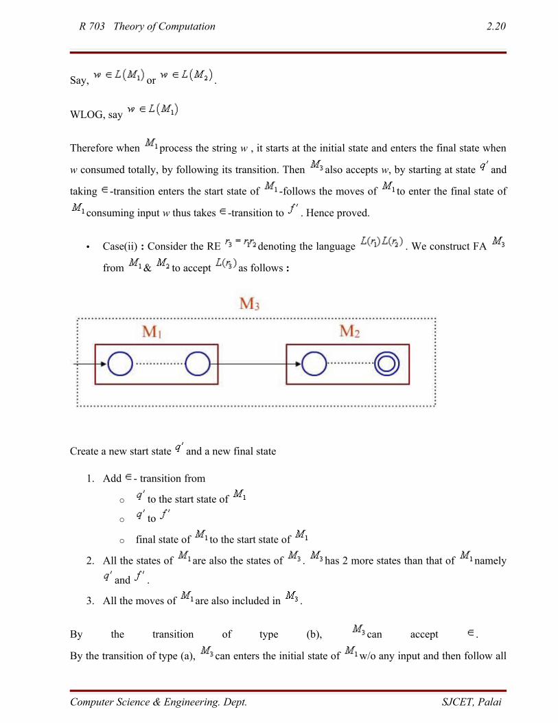
• Case(ii) : Consider the RE denoting the language . We construct FA

from & to accept as follows :

Create a new start state and a new final state

1. Add - transition from

o to the start state of

o to

o final state of to the start state of

2. All the states of are also the states of . has 2 more states than that of namely

and .

3. All the moves of are also included in .

By the transition of type (b), can accept .

By the transition of type (a), can enters the initial state of w/o any input and then follow all



kinds moves of to enter the final state of and then following -transition can enter .

Hence if any is accepted by then w is also accepted by . By the transition of type (b),

strings accepted by can be repeated by any no of times & thus accepted by . Hence

accepts and any string accepted by repeated (i.e. concatenated) any no of times. Hence

• Case(iv) : Let =( ). Then the FA is also the FA for ( ), since the use of parentheses does not change the language denoted by the expression.

iv) Conversion of Finite Automata to Regular Expression by Elimination of States

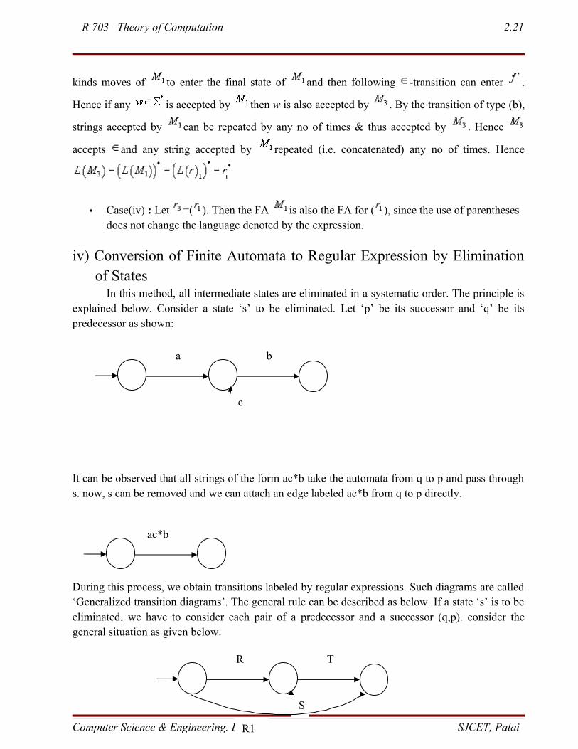
In this method, all intermediate states are eliminated in a systematic order. The principle is explained below. Consider a state ‘s’ to be eliminated. Let ‘p’ be its successor and ‘q’ be its predecessor as shown:

It can be observed that all strings of the form ac*b take the automata from q to p and pass through s. now, s can be removed and we can attach an edge labeled ac*b from q to p directly.

During this process, we obtain transitions labeled by regular expressions. Such diagrams are called ‘Generalized transition diagrams’. The general rule can be described as below. If a state ‘s’ is to be eliminated, we have to consider each pair of a predecessor and a successor (q,p). consider the general situation as given below.


ac*b

ba

c

TR

S

R1


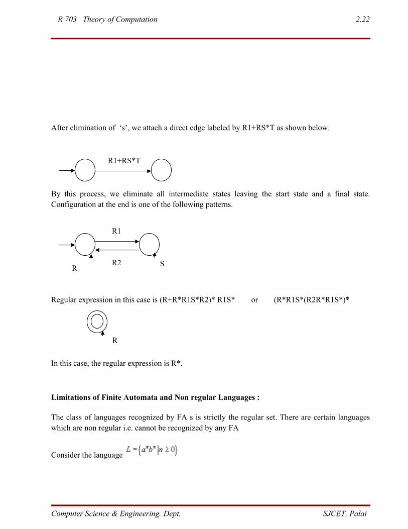
After elimination of ‘s’, we attach a direct edge labeled by R1+RS*T as shown below.

By this process, we eliminate all intermediate states leaving the start state and a final state. Configuration at the end is one of the following patterns.

Regular expression in this case is (R+R*R1S*R2)* R1S* or (R*R1S*(R2R*R1S*)*

In this case, the regular expression is R*.

Limitations of Finite Automata and Non regular Languages :

The class of languages recognized by FA s is strictly the regular set. There are certain languages which are non regular i.e. cannot be recognized by any FA

Consider the language


R1+RS*T

R1

SR

R2

R


In order to accept is language, we find that, an automaton seems to need to remember when passing

the center point between a's and b's how many a's it has seen so far. Because it should have to

compare that with the number of b's to either accept (when the two numbers are same) or reject (when they are not same) the input string.

But the number of a's is not limited and may be much larger than the number of states since the string may be arbitrarily long. So, the amount of information the automaton need to remember is unbounded.

A finite automaton cannot remember this with only finite memory (i.e. finite number of states).

The fact that FA s have finite memory imposes some limitations on the structure of the languages recognized. Inductively, we can say that a language is regular only if in processing any string in this language, the information that has to be remembered at any point is strictly limited. The

argument given above to show that is non regular is informal. We now present a formal

method for showing that certain languages such as are non regular.

Pumping Lemma for regular languages

In the theory of formal languages, a pumping lemma states that any language of a given class can be "pumped" and still belong to that class. A language can be pumped if any sufficiently long string in the language can be broken into pieces that can be repeated to produce an even longer string in the language. Thus, if there is a pumping lemma for a given language class, any language in the class will contain an infinite set of finite strings all produced by a simple rule given by the lemma. The two most important examples are the pumping lemma for regular languages and the pumping lemma for context-free languages. Unlike theorems, lemmas are specifically intended to facilitate streamlined proofs. These two lemmas are used to determine if a particular language is not in a given language class. However, they cannot be used to determine if a language is in a given class, since satisfying the pumping lemma is a necessary, but not sufficient, condition for class membership.

Pumping Lemma :

Let L be a regular language. Then the following property olds for L.

There exists a number (called, the pumping length), where, if w is any string in L of length at

least k i.e. , then w may be divided into three sub strings w = xyz, satisfying the following conditions:

1. i.e.


http://en.wikipedia.org/wiki/Necessary_and_sufficient

http://en.wikipedia.org/wiki/Lemma_(mathematics)

http://en.wikipedia.org/wiki/Theorem

http://en.wikipedia.org/wiki/Context-free_language

http://en.wikipedia.org/wiki/Regular_language



2.

3.

Proof : Since L is regular, there exists a DFA that recognizes it, i.e. L = L(M) . Let the number of states in M is n.

Say,

Consider a string such that (we consider the language L to be infinite and hence such

a string can always be found). If no string of such length is found to be in L , then the lemma becomes vacuously true.

Since . Say while processing the string w , the DFA M goes through a sequence of states of states. Assume the sequence to be

Since , the number of states in the above sequence must be greater than n + 1. But number

of states in M is only n. hence, by pigeonhole principle at least one state must be repeated.

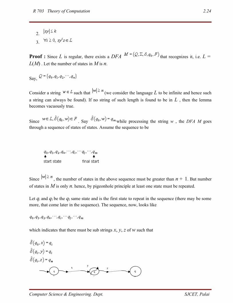
Let qi and ql be the ql same state and is the first state to repeat in the sequence (there may be some more, that come later in the sequence). The sequence, now, looks like

which indicates that there must be sub strings x, y, z of w such that


q

0

q

i

q

m

xy

z


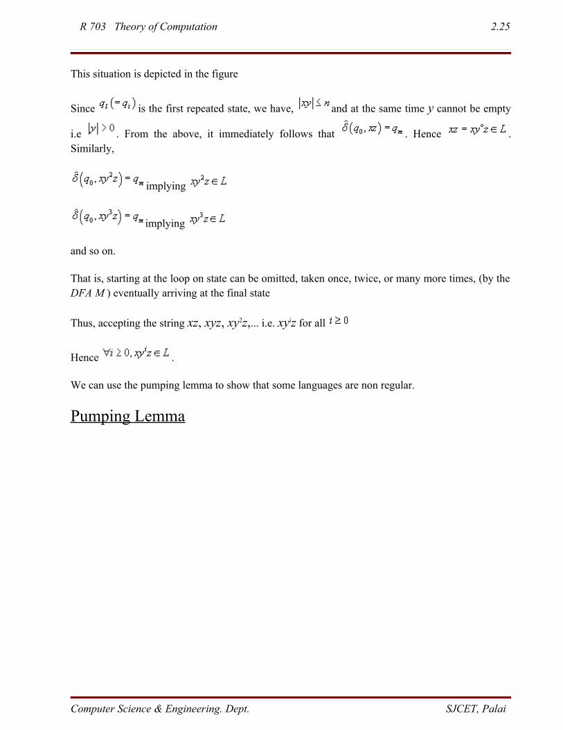
This situation is depicted in the figure

Since is the first repeated state, we have, and at the same time y cannot be empty

i.e . From the above, it immediately follows that . Hence . Similarly,

implying

implying

and so on.

That is, starting at the loop on state can be omitted, taken once, twice, or many more times, (by the DFA M ) eventually arriving at the final state

Thus, accepting the string xz, xyz, xy2z,... i.e. xyiz for all

Hence .

We can use the pumping lemma to show that some languages are non regular.

Pumping Lemma



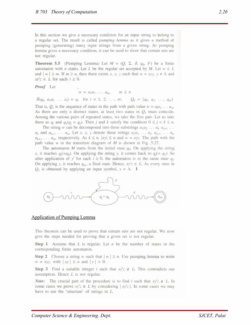
Application of Pumping Lemma



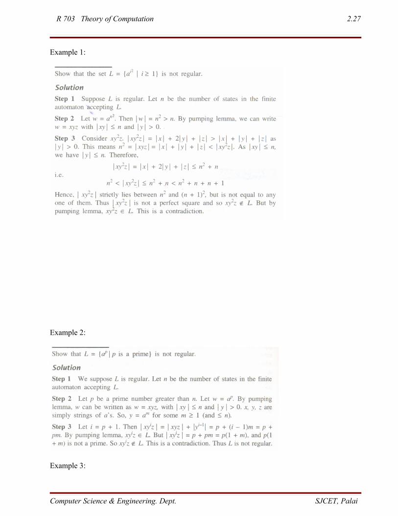
Example 1:

Example 2:

Example 3:



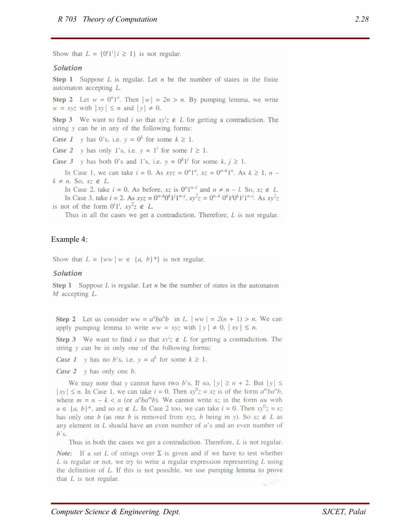
Example 4:



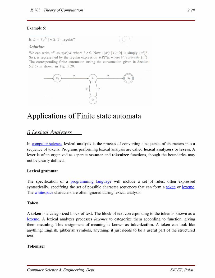
Example 5:

Applications of Finite state automata

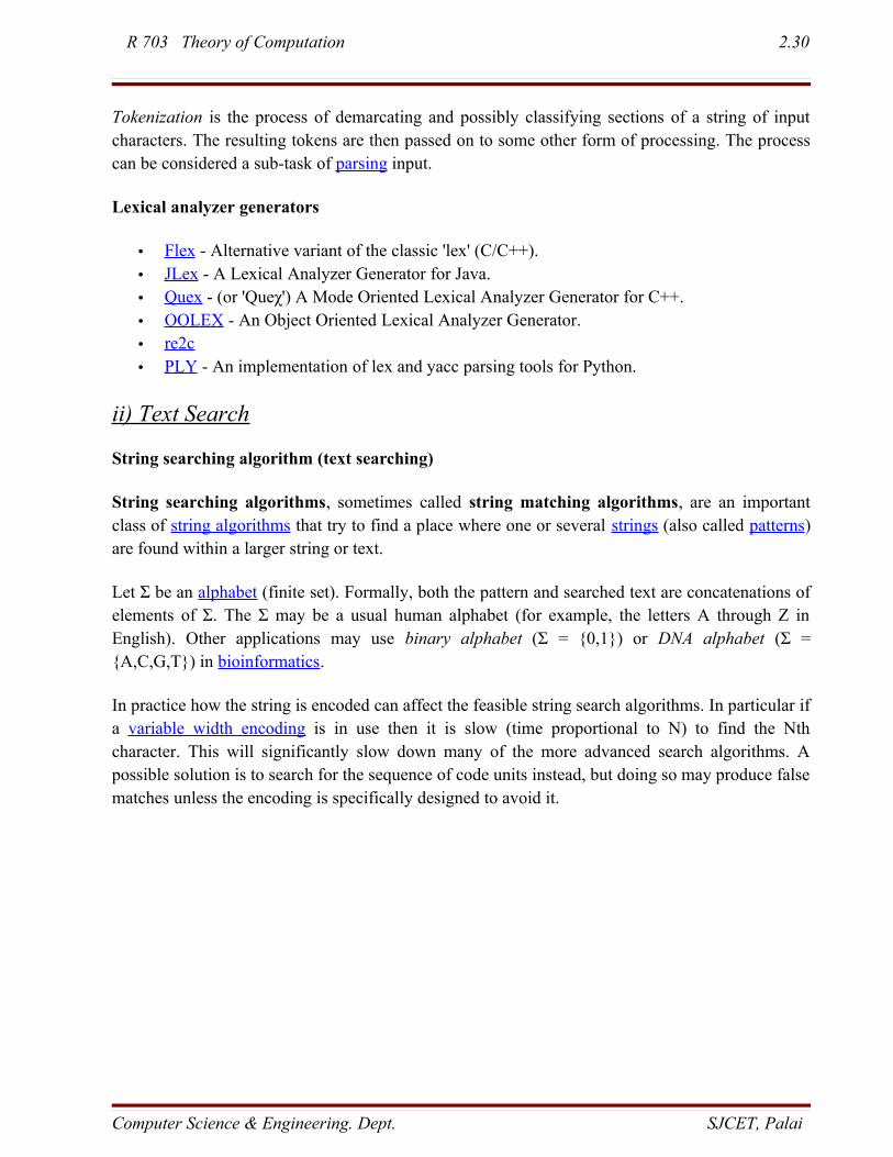
i) Lexical Analyzers

In computer science, lexical analysis is the process of converting a sequence of characters into a sequence of tokens. Programs performing lexical analysis are called lexical analyzers or lexers. A lexer is often organized as separate scanner and tokenizer functions, though the boundaries may not be clearly defined.

Lexical grammar

The specification of a programming language will include a set of rules, often expressed syntactically, specifying the set of possible character sequences that can form a token or lexeme. The whitespace characters are often ignored during lexical analysis.

Token

A token is a categorized block of text. The block of text corresponding to the token is known as a lexeme. A lexical analyzer processes lexemes to categorize them according to function, giving them meaning. This assignment of meaning is known as tokenization. A token can look like anything: English, gibberish symbols, anything; it just needs to be a useful part of the structured text.

Tokenizer


http://en.wikipedia.org/wiki/Lexeme

http://en.wikipedia.org/wiki/Whitespace

http://en.wikipedia.org/wiki/Lexeme

http://en.wikipedia.org/wiki/Token

http://en.wikipedia.org/wiki/Programming_language

http://en.wikipedia.org/wiki/Computer_science


Tokenization is the process of demarcating and possibly classifying sections of a string of input characters. The resulting tokens are then passed on to some other form of processing. The process can be considered a sub-task of parsing input.

Lexical analyzer generators

• Flex - Alternative variant of the classic 'lex' (C/C++). • JLex - A Lexical Analyzer Generator for Java. • Quex - (or 'Queχ') A Mode Oriented Lexical Analyzer Generator for C++. • OOLEX - An Object Oriented Lexical Analyzer Generator. • re2c • PLY - An implementation of lex and yacc parsing tools for Python.

ii) Text Search

String searching algorithm (text searching)

String searching algorithms, sometimes called string matching algorithms, are an important class of string algorithms that try to find a place where one or several strings (also called patterns) are found within a larger string or text.

Let Σ be an alphabet (finite set). Formally, both the pattern and searched text are concatenations of elements of Σ. The Σ may be a usual human alphabet (for example, the letters A through Z in English). Other applications may use binary alphabet (Σ = {0,1}) or DNA alphabet (Σ = {A,C,G,T}) in bioinformatics.

In practice how the string is encoded can affect the feasible string search algorithms. In particular if a variable width encoding is in use then it is slow (time proportional to N) to find the Nth character. This will significantly slow down many of the more advanced search algorithms. A possible solution is to search for the sequence of code units instead, but doing so may produce false matches unless the encoding is specifically designed to avoid it.


http://en.wikipedia.org/wiki/Variable_width_encoding

http://en.wikipedia.org/wiki/Bioinformatics

http://en.wikipedia.org/wiki/Alphabet_(computer_science)

http://en.wikipedia.org/wiki/Pattern

http://en.wikipedia.org/wiki/String_(computer_science)

http://en.wikipedia.org/wiki/String_algorithm

http://en.wikipedia.org/w/index.php?title=PLY_(lexical_analyser)&action=edit&redlink=1

http://en.wikipedia.org/w/index.php?title=Re2c_(lexical_analyser)&action=edit&redlink=1

http://en.wikipedia.org/w/index.php?title=OOLEX&action=edit&redlink=1

http://en.wikipedia.org/wiki/Quex

http://en.wikipedia.org/wiki/JLex

http://en.wikipedia.org/wiki/Flex_lexical_analyser

http://en.wikipedia.org/wiki/Parsing



Documents

Introduction to Automata Theory - Notesvillagenotesvillage.com/upload/MODULE II.pdfR 703 Theory of Computation 2.5 Deterministic Finite Automata can be defined as M=(Q,Σ,δ,q0,F)