Embed Size (px)
Citation preview

Treatment variation Sums of squares Normal sampling models
Introduction to ANOVAApplied Statistics and Experimental Design
Chapter 5
Peter Hoff
Statistics, Biostatistics and the CSSSUniversity of Washington

Treatment variation Sums of squares Normal sampling models
Response time data
Background: Psychologists are interested in how learning methods affectshort-term memory.
Hypothesis: Different learning methods may result in different recall time.
Treatments: 5 different learning methods (A, B, C, D, E).
Experimental design: (CRD) 20 male undergraduate students were randomlyassigned to one of the 5 treatments, so that there are 4 students assignedto each treatment. After a learning period, the students were given cuesand asked to recall a set of words. Mean recall time for each student wasrecorded in seconds.
Results:
Treatment sample mean sample sdA 6.88 0.76B 5.41 0.84C 6.59 1.37D 5.46 0.41E 5.64 0.83
Question: Is treatment a source of variation?

Treatment variation Sums of squares Normal sampling models
Response time data
●
●
●●
●
●
●
●
●
●
●
●
●
●●●
●
●
●
●
56
78
treatment
resp
onse
tim
e (s
econ
ds)
A B C D E

Treatment variation Sums of squares Normal sampling models
Possible data analysis method
Test H0i1 i2 : µi1 = µi2 versus H1i1 i2 : µi1 6= µi2
for each of the`
52
´= 10 possible pairwise comparisons.
Reject a hypothesis if the associated p-value ≤ α.
Problem: If there is no treatment effect at all, then
Pr(reject H0i1 i2 |H0i1 i2 true) = α
Pr(reject any H0i1 i2 | all H0i1 i2 true ) = 1− Pr( accept all H0i1 i2 | all H0i1 i2 true )
≈ 1−Yi<j
(1− α)
If α = 0.05, then
Pr(reject one or more H0i1 i2 | all H0i1 i2 true ) ≈ 1− .9510 = 0.40

Treatment variation Sums of squares Normal sampling models
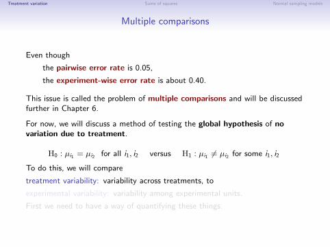
Multiple comparisons
Even though
the pairwise error rate is 0.05,
the experiment-wise error rate is about 0.40.
This issue is called the problem of multiple comparisons and will be discussedfurther in Chapter 6.
For now, we will discuss a method of testing the global hypothesis of novariation due to treatment.
H0 : µi1 = µi2 for all i1, i2 versus H1 : µi1 6= µi2 for some i1, i2
To do this, we will compare
treatment variability: variability across treatments, to
experimental variability: variability among experimental units.
First we need to have a way of quantifying these things.

Treatment variation Sums of squares Normal sampling models
Multiple comparisons
Even though
the pairwise error rate is 0.05,
the experiment-wise error rate is about 0.40.
This issue is called the problem of multiple comparisons and will be discussedfurther in Chapter 6.
For now, we will discuss a method of testing the global hypothesis of novariation due to treatment.
H0 : µi1 = µi2 for all i1, i2 versus H1 : µi1 6= µi2 for some i1, i2
To do this, we will compare
treatment variability: variability across treatments, to
experimental variability: variability among experimental units.
First we need to have a way of quantifying these things.

Treatment variation Sums of squares Normal sampling models
A model for treatment variation
Data:yij = measurement from the jth replicate under the ith treatment.
i = 1, . . . ,m indexes treatmentsj = 1, . . . , n indexes observations or replicates.
Treatment means model:
yij = µi + εij
E[εij ] = 0
Var[εij ] = σ2
µi is the ith treatment mean,
εij ’s represent within treatment variation, also known as error or noise.

Treatment variation Sums of squares Normal sampling models
A model for treatment variation
Data:yij = measurement from the jth replicate under the ith treatment.i = 1, . . . ,m indexes treatments
j = 1, . . . , n indexes observations or replicates.
Treatment means model:
yij = µi + εij
E[εij ] = 0
Var[εij ] = σ2
µi is the ith treatment mean,
εij ’s represent within treatment variation, also known as error or noise.

Treatment variation Sums of squares Normal sampling models
A model for treatment variation
Data:yij = measurement from the jth replicate under the ith treatment.i = 1, . . . ,m indexes treatmentsj = 1, . . . , n indexes observations or replicates.
Treatment means model:
yij = µi + εij
E[εij ] = 0
Var[εij ] = σ2
µi is the ith treatment mean,
εij ’s represent within treatment variation, also known as error or noise.

Treatment variation Sums of squares Normal sampling models
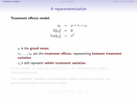
A reparameterization
Treatment effects model:
yij = µ+ τi + εij
E[εij ] = 0
Var[εij ] = σ2
µ is the grand mean;
τ1, . . . , τm are the treatment effects, representing between treatmentvariation
εij ’s still represent within treatment variation.
In this model, we typically restrictPτi = 0, otherwise the model is
overparameterized.
The treatment means and treatment effects models represent twoparameterizations of the same model:
µi = µ+ τi ⇔ τi = µi − µ

Treatment variation Sums of squares Normal sampling models
A reparameterization
Treatment effects model:
yij = µ+ τi + εij
E[εij ] = 0
Var[εij ] = σ2
µ is the grand mean;
τ1, . . . , τm are the treatment effects, representing between treatmentvariation
εij ’s still represent within treatment variation.
In this model, we typically restrictPτi = 0, otherwise the model is
overparameterized.
The treatment means and treatment effects models represent twoparameterizations of the same model:
µi = µ+ τi ⇔ τi = µi − µ

Treatment variation Sums of squares Normal sampling models
Null (or reduced) model
yij = µ+ εij
E[εij ] = 0
Var[εij ] = σ2
This is a special case of the above two models with
• µ = µ1 = · · ·µm , or equivalently
• τi = 0 for all i .
In this model, there is no variation due to treatment.
Two models:• Treament variation model
• Treatment means parameterization: yi,j = µi + εi,j• Treatment effects parameterization: yi,j = µ+ τj + εi,j
• No treatment variation model• Null model: yi,j = µ+ εi,j

Treatment variation Sums of squares Normal sampling models
Model Fitting
What are good estimates of the parameters?
One criteria used to evaluate different values of µ = {µ1, . . . , µm} is the
least squares criterion : SSE(µ) =mX
i=1
nXj=1
(yij − µi )2
The value of µ that minimizes SSE(µ) is
called the least-squares estimate.
and will be denoted µ.

Treatment variation Sums of squares Normal sampling models
Estimating treatment means:
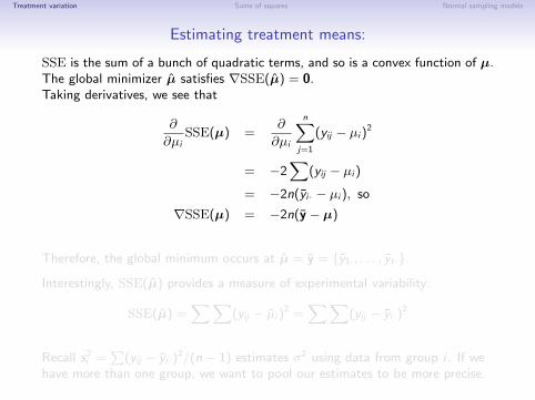
SSE is the sum of a bunch of quadratic terms, and so is a convex function of µ.The global minimizer µ satisfies ∇SSE(µ) = 0.Taking derivatives, we see that
∂
∂µiSSE(µ) =
∂
∂µi
nXj=1
(yij − µi )2
= −2X
(yij − µi )
= −2n(yi· − µi ), so
∇SSE(µ) = −2n(y − µ)
Therefore, the global minimum occurs at µ = y = {y1·, . . . , yt·}.
Interestingly, SSE(µ) provides a measure of experimental variability:
SSE(µ) =XX
(yij − µi )2 =
XX(yij − yi·)
2
Recall s2i =
P(yij − yi·)
2/(n − 1) estimates σ2 using data from group i . If wehave more than one group, we want to pool our estimates to be more precise.

Treatment variation Sums of squares Normal sampling models
Estimating treatment means:
SSE is the sum of a bunch of quadratic terms, and so is a convex function of µ.The global minimizer µ satisfies ∇SSE(µ) = 0.Taking derivatives, we see that
∂
∂µiSSE(µ) =
∂
∂µi
nXj=1
(yij − µi )2
= −2X
(yij − µi )
= −2n(yi· − µi ), so
∇SSE(µ) = −2n(y − µ)
Therefore, the global minimum occurs at µ = y = {y1·, . . . , yt·}.
Interestingly, SSE(µ) provides a measure of experimental variability:
SSE(µ) =XX
(yij − µi )2 =
XX(yij − yi·)
2
Recall s2i =
P(yij − yi·)
2/(n − 1) estimates σ2 using data from group i . If wehave more than one group, we want to pool our estimates to be more precise.
Treatment variation Sums of squares Normal sampling models
Estimating the variance
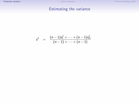
s2 =(n − 1)s2
1 + · · ·+ (n − 1)s2m
(n − 1) + · · ·+ (n − 1)
=
P(y1j − y1·)
2 + · · ·+P
(y1j − y1·)2
m(n − 1)
=
PP(yij − µi )
2
m(n − 1)
=SSE(µ)
m(n − 1)≡ MSE

Treatment variation Sums of squares Normal sampling models
Estimating the variance
s2 =(n − 1)s2
1 + · · ·+ (n − 1)s2m
(n − 1) + · · ·+ (n − 1)
=
P(y1j − y1·)
2 + · · ·+P
(y1j − y1·)2
m(n − 1)
=
PP(yij − µi )
2
m(n − 1)
=SSE(µ)
m(n − 1)≡ MSE

Treatment variation Sums of squares Normal sampling models
Estimating the variance
s2 =(n − 1)s2
1 + · · ·+ (n − 1)s2m
(n − 1) + · · ·+ (n − 1)
=
P(y1j − y1·)
2 + · · ·+P
(y1j − y1·)2
m(n − 1)
=
PP(yij − µi )
2
m(n − 1)
=SSE(µ)
m(n − 1)≡ MSE

Treatment variation Sums of squares Normal sampling models
Estimating the variance
s2 =(n − 1)s2
1 + · · ·+ (n − 1)s2m
(n − 1) + · · ·+ (n − 1)
=
P(y1j − y1·)
2 + · · ·+P
(y1j − y1·)2
m(n − 1)
=
PP(yij − µi )
2
m(n − 1)
=SSE(µ)
m(n − 1)≡ MSE

Treatment variation Sums of squares Normal sampling models
Interpreting sample estimates
The values µ and s2 have various interpretations depending on assumptions.
Consider the following assumptions:
A0: Data are independently sampled from their respective populations
A1: Populations have the same variance
A2: Populations are normally distributed
Then
A0 → µ is an unbiased estimator of µ
A0+A1 → s2 is an unbiased estimator of σ2
A0+A1+A2 →(µ, s2) are the minimum variance unbiased estimators of (µ, σ2)(µ, n−1
ns2) are the maximum likelihood estimators of (µ, σ2)

Treatment variation Sums of squares Normal sampling models
Within-treatment variability
SSE(µ) ≡ SSE is a measure of within treatment variability:
SSE =mX
i=1
nXj=1
(yij − yi·)2
It is the sum of squared deviation of observation values from their group mean.
MSE = SSE/m(n − 1) =1
m(s2
1 + · · ·+ s2m)
Clearly MSE is a measure of average (or mean) within-treatment variability.

Treatment variation Sums of squares Normal sampling models
Between-treatment variabilityThe analogous measure of between treatment variability is
SST =mX
i=1
nXj=1
(yi· − y··)2 = n
mXi=1
(yi· − y··)2
where
y·· =1
mn
XXyij
=1
m(y1 + · · ·+ ym)
is the grand mean of the sample.
We call SST the treatment sum of squares.We also define MST = SST/(m − 1) as
the treatment mean squares or
the mean squares (due to) treatment.
Note MST is simply n times the sample variance of the sample means:
MST = n ×
"1
m − 1
mXi=1
(yi· − y··)2
#

Treatment variation Sums of squares Normal sampling models
Testing hypothesis with MSE and MST
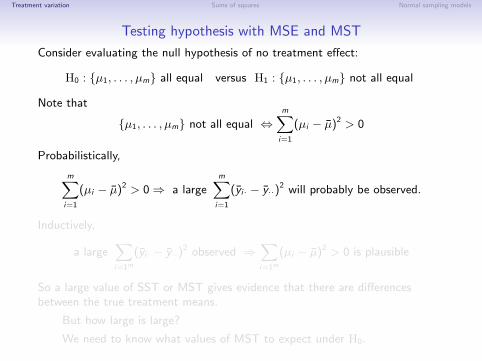
Consider evaluating the null hypothesis of no treatment effect:
H0 : {µ1, . . . , µm} all equal versus H1 : {µ1, . . . , µm} not all equal
Note that
{µ1, . . . , µm} not all equal ⇔mX
i=1
(µi − µ)2 > 0
Probabilistically,
mXi=1
(µi − µ)2 > 0⇒ a largemX
i=1
(yi· − y··)2 will probably be observed.
Inductively,
a largeXi=1m
(yi· − y··)2 observed ⇒
Xi=1m
(µi − µ)2 > 0 is plausible
So a large value of SST or MST gives evidence that there are differencesbetween the true treatment means.
But how large is large?
We need to know what values of MST to expect under H0.

Treatment variation Sums of squares Normal sampling models
Testing hypothesis with MSE and MST
Consider evaluating the null hypothesis of no treatment effect:
H0 : {µ1, . . . , µm} all equal versus H1 : {µ1, . . . , µm} not all equal
Note that
{µ1, . . . , µm} not all equal ⇔mX
i=1
(µi − µ)2 > 0
Probabilistically,
mXi=1
(µi − µ)2 > 0⇒ a largemX
i=1
(yi· − y··)2 will probably be observed.
Inductively,
a largeXi=1m
(yi· − y··)2 observed ⇒
Xi=1m
(µi − µ)2 > 0 is plausible
So a large value of SST or MST gives evidence that there are differencesbetween the true treatment means.
But how large is large?
We need to know what values of MST to expect under H0.

Treatment variation Sums of squares Normal sampling models
MST under the null
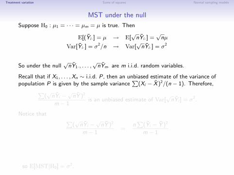
Suppose H0 : µ1 = · · · = µm = µ is true. Then
E[(Yi·] = µ → E[√
nYi·] =√
nµ
Var[Yi·] = σ2/n → Var[√
nYi·] = σ2
So under the null√
nY1·, . . . ,√
nYm· are m i.i.d. random variables.
Recall that if X1, . . . ,Xn ∼ i.i.d. P, then an unbiased estimate of the variance ofpopulation P is given by the sample variance
P(Xi − X )2/(n − 1). Therefore,P
(√
nYi −√
nY )2
m − 1is an unbiased estimate of Var[
√nYi ] = σ2.
Notice that P(√
nYi −√
nY )2
m − 1=
nP
(Yi − Y )2
m − 1
=SST
m − 1= MST,
so E[MST|H0] = σ2.

Treatment variation Sums of squares Normal sampling models
MST under the null
Suppose H0 : µ1 = · · · = µm = µ is true. Then
E[(Yi·] = µ → E[√
nYi·] =√
nµ
Var[Yi·] = σ2/n → Var[√
nYi·] = σ2
So under the null√
nY1·, . . . ,√
nYm· are m i.i.d. random variables.
Recall that if X1, . . . ,Xn ∼ i.i.d. P, then an unbiased estimate of the variance ofpopulation P is given by the sample variance
P(Xi − X )2/(n − 1). Therefore,P
(√
nYi −√
nY )2
m − 1is an unbiased estimate of Var[
√nYi ] = σ2.
Notice that P(√
nYi −√
nY )2
m − 1=
nP
(Yi − Y )2
m − 1
=SST
m − 1= MST,
so E[MST|H0] = σ2.

Treatment variation Sums of squares Normal sampling models
MST under the null
Suppose H0 : µ1 = · · · = µm = µ is true. Then
E[(Yi·] = µ → E[√
nYi·] =√
nµ
Var[Yi·] = σ2/n → Var[√
nYi·] = σ2
So under the null√
nY1·, . . . ,√
nYm· are m i.i.d. random variables.
Recall that if X1, . . . ,Xn ∼ i.i.d. P, then an unbiased estimate of the variance ofpopulation P is given by the sample variance
P(Xi − X )2/(n − 1). Therefore,P
(√
nYi −√
nY )2
m − 1is an unbiased estimate of Var[
√nYi ] = σ2.
Notice that P(√
nYi −√
nY )2
m − 1=
nP
(Yi − Y )2
m − 1
=SST
m − 1
= MST,
so E[MST|H0] = σ2.

Treatment variation Sums of squares Normal sampling models
MST under the null
Suppose H0 : µ1 = · · · = µm = µ is true. Then
E[(Yi·] = µ → E[√
nYi·] =√
nµ
Var[Yi·] = σ2/n → Var[√
nYi·] = σ2
So under the null√
nY1·, . . . ,√
nYm· are m i.i.d. random variables.
Recall that if X1, . . . ,Xn ∼ i.i.d. P, then an unbiased estimate of the variance ofpopulation P is given by the sample variance
P(Xi − X )2/(n − 1). Therefore,P
(√
nYi −√
nY )2
m − 1is an unbiased estimate of Var[
√nYi ] = σ2.
Notice that P(√
nYi −√
nY )2
m − 1=
nP
(Yi − Y )2
m − 1
=SST
m − 1= MST,
so E[MST|H0] = σ2.

Treatment variation Sums of squares Normal sampling models
MST under the null
Suppose H0 : µ1 = · · · = µm = µ is true. Then
E[(Yi·] = µ → E[√
nYi·] =√
nµ
Var[Yi·] = σ2/n → Var[√
nYi·] = σ2
So under the null√
nY1·, . . . ,√
nYm· are m i.i.d. random variables.
Recall that if X1, . . . ,Xn ∼ i.i.d. P, then an unbiased estimate of the variance ofpopulation P is given by the sample variance
P(Xi − X )2/(n − 1). Therefore,P
(√
nYi −√
nY )2
m − 1is an unbiased estimate of Var[
√nYi ] = σ2.
Notice that P(√
nYi −√
nY )2
m − 1=
nP
(Yi − Y )2
m − 1
=SST
m − 1= MST,
so E[MST|H0] = σ2.
Treatment variation Sums of squares Normal sampling models
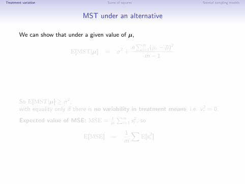
MST under an alternative
We can show that under a given value of µ,
E[MST|µ] = σ2 +nPm
i=1(µi − µ)2
m − 1
= σ2 + n
Pmi=1 τ
2i
m − 1
≡ σ2 + nv 2τ
So E[MST|µ] ≥ σ2,with equality only if there is no variability in treatment means, i.e. v 2
τ = 0.
Expected value of MSE: MSE = 1m
Pmi=1 s2
i , so
E[MSE] =1
m
XE[s2
i ]
=1
m
Xσ2 = σ2

Treatment variation Sums of squares Normal sampling models
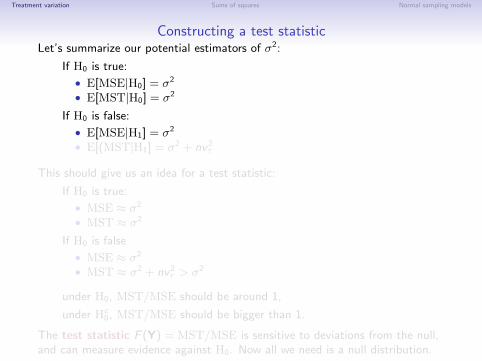
Constructing a test statisticLet’s summarize our potential estimators of σ2:
If H0 is true:
• E[MSE|H0] = σ2
• E[MST|H0] = σ2
If H0 is false:
• E[MSE|H1] = σ2
• E[(MST|H1] = σ2 + nv 2τ
This should give us an idea for a test statistic:
If H0 is true:
• MSE ≈ σ2
• MST ≈ σ2
If H0 is false
• MSE ≈ σ2
• MST ≈ σ2 + nv 2τ > σ2
under H0, MST/MSE should be around 1,
under Hc0, MST/MSE should be bigger than 1.
The test statistic F (Y) = MST/MSE is sensitive to deviations from the null,and can measure evidence against H0. Now all we need is a null distribution.

Treatment variation Sums of squares Normal sampling models
Constructing a test statisticLet’s summarize our potential estimators of σ2:
If H0 is true:
• E[MSE|H0] = σ2
• E[MST|H0] = σ2
If H0 is false:
• E[MSE|H1] = σ2
• E[(MST|H1] = σ2 + nv 2τ
This should give us an idea for a test statistic:
If H0 is true:
• MSE ≈ σ2
• MST ≈ σ2
If H0 is false
• MSE ≈ σ2
• MST ≈ σ2 + nv 2τ > σ2
under H0, MST/MSE should be around 1,
under Hc0, MST/MSE should be bigger than 1.
The test statistic F (Y) = MST/MSE is sensitive to deviations from the null,and can measure evidence against H0. Now all we need is a null distribution.

Treatment variation Sums of squares Normal sampling models
Example (response times):
y b a r . t<−t a p p l y ( y , x , mean )s2 . t<−t a p p l y ( y , x , v a r )
SSE<− sum ( ( n−1)∗ s2 . t )SST<− n∗sum ( ( y b a r . t−mean ( y ) ) ˆ 2 )
MSE<−SSE /(m∗(n−1))MST<−SST/(m−1)
> SSE[ 1 ] 12 .0379
> SST[ 1 ] 7 .55032
> MSE[ 1 ] 0 .8025267
> MST[ 1 ] 1 .88758
It is customary to summarize these calculations in a table:
Source of variation Sums of Squares Mean Squares F -ratioTreatment 7.55 1.89 2.35Noise 12.04 0.80

Treatment variation Sums of squares Normal sampling models
Example (response times):
The F -ratio deviates a bit from 1. Possible explanations:
• H1: The F -value is a result of actual differences between treatments.
• H0: The F -value is a result of a chance assignment of treatments , eg. theslow students were randomized to A, the fast students to D.
To evaluate H0 we look at how likely such a treatment assignment is.
F . obs<−anova ( lm ( y ˜ as . f a c t o r ( x ) ) ) $F [ 1 ]
> F . obs[ 1 ] 2 .352046
$s e t . s e e d ( 1 )F . n u l l <−NULLf o r ( nsim i n 1 : 1 0 0 0 ){
x . sim<−sample ( x )F . n u l l <−c ( F . n u l l , anova ( lm ( y ˜ as . f a c t o r ( x . s im ) ) ) $F [ 1 ] )
}$> mean ( F . n u l l >=F . obs )[ 1 ] 0 . 1 0 2

Treatment variation Sums of squares Normal sampling models
Randomization test
F0 2 4 6 8
0.0
0.2
0.4
0.6
Observed between-group variation is larger than within-group variation,but not substantially larger than the types of F -statistics we’d expect to get ifthe null hypothesis were true.

Treatment variation Sums of squares Normal sampling models
Randomization test
F0 2 4 6 8
0.0
0.2
0.4
0.6
Observed between-group variation is larger than within-group variation,but not substantially larger than the types of F -statistics we’d expect to get ifthe null hypothesis were true.

Treatment variation Sums of squares Normal sampling models
Partitioning sums of squares
Informally, we can think about the total variation in a datasets as follows:
Total variability = variability due to treatment + variability due to other things
= between treatment variability + within treatment variability
This can in fact be made formal:
SSTotal ≡mX
i=1
nXj=1
(yij − y··)2 = SST + SSE
Proof:mX
i=1
nXj=1
(yij − y··)2 =
Xi
Xj
[(yij − yi·) + (yi· − y··)]2
=X
i
Xj
˘(yij − yi·)
2 + 2(yij − yi·)(yi· − y··) + (yi· − y··)2¯
=X
i
Xj
(yij − yi·)2 +
Xi
Xj
2(yij − yi·)(yi· − y··) +X
i
Xj
(yi· − y··)2
= (1) + (2) + (3)

Treatment variation Sums of squares Normal sampling models
Partitioning sums of squares
Informally, we can think about the total variation in a datasets as follows:
Total variability = variability due to treatment + variability due to other things= between treatment variability + within treatment variability
This can in fact be made formal:
SSTotal ≡mX
i=1
nXj=1
(yij − y··)2 = SST + SSE
Proof:mX
i=1
nXj=1
(yij − y··)2 =
Xi
Xj
[(yij − yi·) + (yi· − y··)]2
=X
i
Xj
˘(yij − yi·)
2 + 2(yij − yi·)(yi· − y··) + (yi· − y··)2¯
=X
i
Xj
(yij − yi·)2 +
Xi
Xj
2(yij − yi·)(yi· − y··) +X
i
Xj
(yi· − y··)2
= (1) + (2) + (3)

Treatment variation Sums of squares Normal sampling models
Partitioning sums of squares
(1) =P
i
Pj(yij − yi·)
2 = SSE
(3) =P
i
Pj(yi· − y··)
2 = nP
i (yi· − y··)2 = SST
(2) = 2P
i
Pj(yij − yi·)(yi· − y··) = 2
Pi (yi· − y··)
Pj(yij − yi·)
but note that Xj
(yij − yi·) = (X
j
yij)− nyi,·
= nyi,· − nyi,· = 0
for all j .
Therefore (2) = 0 and we have
total sum of squared deviations from grand mean = between trt sums of squares +within trt sums of squares
or more succinctly,SSTotal = SST + SSE.
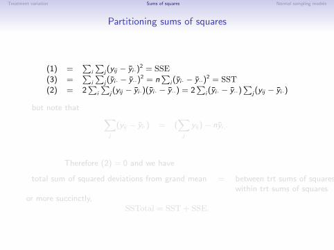

Treatment variation Sums of squares Normal sampling models
Partitioning sums of squares
(1) =P
i
Pj(yij − yi·)
2 = SSE
(3) =P
i
Pj(yi· − y··)
2 = nP
i (yi· − y··)2 = SST
(2) = 2P
i
Pj(yij − yi·)(yi· − y··) = 2
Pi (yi· − y··)
Pj(yij − yi·)
but note that Xj
(yij − yi·) = (X
j
yij)− nyi,·
= nyi,· − nyi,· = 0
for all j . Therefore (2) = 0 and we have
total sum of squared deviations from grand mean = between trt sums of squares +within trt sums of squares
or more succinctly,SSTotal = SST + SSE.
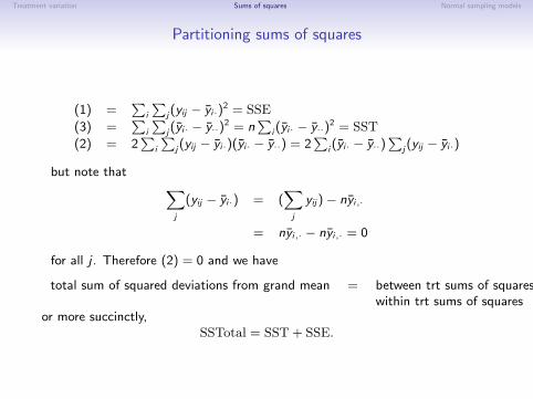
Treatment variation Sums of squares Normal sampling models
Partitioning sums of squares
(1) =P
i
Pj(yij − yi·)
2 = SSE
(3) =P
i
Pj(yi· − y··)
2 = nP
i (yi· − y··)2 = SST
(2) = 2P
i
Pj(yij − yi·)(yi· − y··) = 2
Pi (yi· − y··)
Pj(yij − yi·)
but note that Xj
(yij − yi·) = (X
j
yij)− nyi,·
= nyi,· − nyi,· = 0
for all j . Therefore (2) = 0 and we have
total sum of squared deviations from grand mean = between trt sums of squares +within trt sums of squares
or more succinctly,SSTotal = SST + SSE.

Treatment variation Sums of squares Normal sampling models
Putting it all together:
H0 : µi1 = µi2 for all i1, i2 ⇒ Reduced model : yij = µ+ εijH1 : µi1 6= µi2 for some i1 6= i2 ⇒ Full model : yij = µi + εij
• The fitted value or predicted value of yi,j is yij .• The residual εij is the observed value minus the fitted value, εij = yij − yij .
If we believe H1,• our estimate of µi is µi = yi·• the fitted value of yij is yij = µi = yi·• the residual for (ij) is εij = (yij − yij) = (yij − yi·).• the model lack-of-fit is measured by the “sum of squared errors”:X
i
Xj
(yij − yi·)2 = SSEF
If we believe H0,• our estimate of µ is µ = y··• the fitted value of yij is yij = µ = y··• the residual for (ij) is εij = (yij − yij) = (yij − y··).• the model lack-of-fit in this case isX
i
Xj
(yij − y··)2 = SSER = SSTotal

Treatment variation Sums of squares Normal sampling models
The ANOVA table
The improvement in model fit by including treatment parameters is
error in reduced model - error in full model = improvement in model fit
SSTotal - SSE = SST
The main idea:Variance can be partitioned into parts representing different sources.The variance explained by different sources can be compared and analyzed.This gives rise to the ANOVA table.
ANOVA = Analysis of Variance
Source Deg of Freedom Sums of Squares Mean Squares F-ratioTreatment m − 1 SST MST=SST/(m − 1) MST/MSENoise m(n − 1) SSE MSE=SSE/m(n − 1)
Total mn − 1 SSTotal

Treatment variation Sums of squares Normal sampling models
The ANOVA table
The improvement in model fit by including treatment parameters is
error in reduced model - error in full model = improvement in model fitSSTotal - SSE = SST
The main idea:Variance can be partitioned into parts representing different sources.The variance explained by different sources can be compared and analyzed.This gives rise to the ANOVA table.
ANOVA = Analysis of Variance
Source Deg of Freedom Sums of Squares Mean Squares F-ratioTreatment m − 1 SST MST=SST/(m − 1) MST/MSENoise m(n − 1) SSE MSE=SSE/m(n − 1)
Total mn − 1 SSTotal

Treatment variation Sums of squares Normal sampling models
Reaction time example:
Source of variation Deg of Freedom Sums of Squares Mean Squares F-ratioTreatment 4 7.55 1.89 2.352Noise 15 12.04 0.80Total 19 19.59
Uses of the ANOVA table:
• No model assumptions → a descriptive decomposition of variation.
• Assuming Var[Yij ] = σ2 in all groups →• E[MSE] = σ2
• E[MST] = σ2 + nv2τ , where v2
τ = variance of true group means.
• Assuming trts were randomly assigned → hypothesis tests, p-values.
• Assuming data are random samples from normal population →hypothesis tests, p-values, confidence intervals for parameters, powercalculations.

Treatment variation Sums of squares Normal sampling models
Understanding Degrees of Freedom:
Consider an experiment with m treatments/groups :
Data Group meansy11 . . . , y1n y1·y21 . . . , y2n y2·
......
ym1 . . . , ymn ym·
9>>>>>=>>>>>;y =
ny1 + · · ·+ nym
mn=
y1 + · · ·+ ym
m
We can “decompose” each observation as follows:
yij = y + (yi − y) + (yij − yi )
This leads to
(yij − y) =
(yi − y) + (yij − yi )total variation = between group variation + within group variation
Each observation can be decomposed this way, leading to the decomposition ofthe data vector of length m × n into two parts.
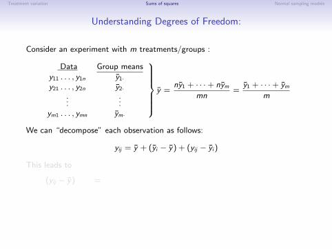

Treatment variation Sums of squares Normal sampling models
Understanding Degrees of Freedom:
Consider an experiment with m treatments/groups :
Data Group meansy11 . . . , y1n y1·y21 . . . , y2n y2·
......
ym1 . . . , ymn ym·
9>>>>>=>>>>>;y =
ny1 + · · ·+ nym
mn=
y1 + · · ·+ ym
m
We can “decompose” each observation as follows:
yij = y + (yi − y) + (yij − yi )
This leads to
(yij − y) = (yi − y) +
(yij − yi )total variation = between group variation + within group variation
Each observation can be decomposed this way, leading to the decomposition ofthe data vector of length m × n into two parts.

Treatment variation Sums of squares Normal sampling models
Understanding Degrees of Freedom:
Consider an experiment with m treatments/groups :
Data Group meansy11 . . . , y1n y1·y21 . . . , y2n y2·
......
ym1 . . . , ymn ym·
9>>>>>=>>>>>;y =
ny1 + · · ·+ nym
mn=
y1 + · · ·+ ym
m
We can “decompose” each observation as follows:
yij = y + (yi − y) + (yij − yi )
This leads to
(yij − y) = (yi − y) + (yij − yi )
total variation = between group variation + within group variation
Each observation can be decomposed this way, leading to the decomposition ofthe data vector of length m × n into two parts.

Treatment variation Sums of squares Normal sampling models
Understanding Degrees of Freedom:
Consider an experiment with m treatments/groups :
Data Group meansy11 . . . , y1n y1·y21 . . . , y2n y2·
......
ym1 . . . , ymn ym·
9>>>>>=>>>>>;y =
ny1 + · · ·+ nym
mn=
y1 + · · ·+ ym
m
We can “decompose” each observation as follows:
yij = y + (yi − y) + (yij − yi )
This leads to
(yij − y) = (yi − y) + (yij − yi )total variation =
between group variation + within group variation
Each observation can be decomposed this way, leading to the decomposition ofthe data vector of length m × n into two parts.

Treatment variation Sums of squares Normal sampling models
Understanding Degrees of Freedom:
Consider an experiment with m treatments/groups :
Data Group meansy11 . . . , y1n y1·y21 . . . , y2n y2·
......
ym1 . . . , ymn ym·
9>>>>>=>>>>>;y =
ny1 + · · ·+ nym
mn=
y1 + · · ·+ ym
m
We can “decompose” each observation as follows:
yij = y + (yi − y) + (yij − yi )
This leads to
(yij − y) = (yi − y) + (yij − yi )total variation = between group variation +
within group variation
Each observation can be decomposed this way, leading to the decomposition ofthe data vector of length m × n into two parts.

Treatment variation Sums of squares Normal sampling models
Understanding Degrees of Freedom:
Consider an experiment with m treatments/groups :
Data Group meansy11 . . . , y1n y1·y21 . . . , y2n y2·
......
ym1 . . . , ymn ym·
9>>>>>=>>>>>;y =
ny1 + · · ·+ nym
mn=
y1 + · · ·+ ym
m
We can “decompose” each observation as follows:
yij = y + (yi − y) + (yij − yi )
This leads to
(yij − y) = (yi − y) + (yij − yi )total variation = between group variation + within group variation
Each observation can be decomposed this way, leading to the decomposition ofthe data vector of length m × n into two parts.

Treatment variation Sums of squares Normal sampling models
ANOVA decomposition
Total Treatment Errory11 − y.. = (y1. − y..) + (y11 − y1.)y12 − y.. = (y1. − y..) + (y12 − y1.)
. = . + .
. = . + .
. = . + .y1n − y.. = (y1. − y..) + (y1n − y1.)y21 − y.. = (y2. − y..) + (y21 − y2.)
. = . + .
. = . + .
. = . + .y2n − y.. = (y2. − y..) + (y2n − y2.)
......
...ym1 − y.. = (ym. − y..) + (ym1 − ym.)
. = . + .
. = . + .
. = . + .ymn − y.. = (ym. − y..) + (ymn − ym.)
SSTotal = SSTrt + SSEmn − 1 = m − 1 + m(n − 1)

Treatment variation Sums of squares Normal sampling models
Understanding degrees of freedom
How do we interpret the degrees of freedom?We’ve seen “degrees of freedom” before, in the definition of a χ2 rv:
dof = number of statistically independent elements in a vector
In the ANOVA table, the dof have a geometric interpretation:
dof = number of components of a vector that can vary independently
To understand this latest definition, consider x1, x2, x3 and x = (x1 + x2 + x3)/3:0@ x1 − xx2 − xx3 − x
1A =
0@ c1
c2
c3
1AHow many degrees of freedom does the vector (c1, c2, c3)T have?
How many components can vary independently, if we know the elements areequal to some numbers minus the average of the numbers?

Treatment variation Sums of squares Normal sampling models
Understanding degrees of freedom
c1 + c2 + c3 = x1 − x + x2 − x − x3 − x
= (x1 + x2 + x3)− 3x
= 3x − 3x
= 0
Thus we must have c1 + c2 = −c3, and so c1, c2, c3 can’t all be independentlyvaried, only two at a time can be arbitrarily changed.
This vector lies in a two-dimensional subspace of R3, has 2 degrees of freedom.In general, 0B@ x1 − x
...xm − x
1CAis an m-dimensional vector in an m − 1 dimensional subspace,having m − 1 degrees of freedom.
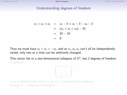

Treatment variation Sums of squares Normal sampling models
Understanding degrees of freedom
Exercise: Return to the vector decomposition of the data and obtain thedegrees of freedom of each component.Note that
• dof = dimension of the space the vector lies in
• SS = squared length of the vector
We will soon see the relationship between the geometric interpretation ofdegrees of freedom and the interpretation involving χ2 random variables.

Treatment variation Sums of squares Normal sampling models
Sums of squares geometry
(to be done on the board)

Treatment variation Sums of squares Normal sampling models
Unbalanced designs
(to be done on the board)

Treatment variation Sums of squares Normal sampling models
Example (Blood coagulation):
N=24 animals were selected from a large population of farm animals.Animals randomly assigned to one of four different diets A, B, C , D.However, due to resource constraints, nA = 4, nB = 6, nC = 6, nD = 8.
A
A
A
A
B
B
B
BBB
C
C
C
CCC
D
D
DDDDD
D
6065
70
diet
coag
ulat
ion
time

Treatment variation Sums of squares Normal sampling models
Inferential questions
• Does diet have an effect on coagulation time?
• If a given diet were assigned to all the animals in the population,what would the distribution of coagulation times be?
• If there is a diet effect, how do the mean coagulation times differ?
The first question we can address with a randomization test.For the second and third we need a sampling model:
yij = µi + εij
ε11 . . . εmnm ∼ i.i.d. normal(0, σ2)
This model implies
• independence of errors
• constant variance
• normally distributed data

Treatment variation Sums of squares Normal sampling models
Sampling model
Another way to write the model is as follows:
yA1, . . . , yA4 ∼ i.i.d. normal(µA, σ2)
yB1, . . . , yB6 ∼ i.i.d. normal(µB , σ2)
yC1, . . . , yC6 ∼ i.i.d. normal(µC , σ2)
yD1, . . . , yD8 ∼ i.i.d. normal(µD , σ2)
So we are viewing the 4 samples under A as a random sample from thepopulation of coagulation times that would be present if all animals got A(and similarly for samples under B, C and D).
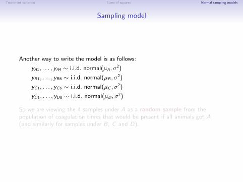

Treatment variation Sums of squares Normal sampling models
Hypothesis testing
> anova ( lm ( c t i m e ˜ d i e t ) )A n a l y s i s o f V a r i a n c e Table
Response : c t i m eDf Sum Sq Mean Sq F v a l u e
d i e t 3 2 2 8 . 0 7 6 . 0 13 .571R e s i d u a l s 20 1 1 2 . 0 5 . 6
The F -statistic is large, but how unlikely is it under H0?
Two viewpoints on null distributions:
• The 24 animals we selected are fixed. Other possible outcomes of theexperiment correspond to different assignments of the treatments.
• The 24 animals we selected are random samples from a larger populationof animals. Other possible outcomes of the experiment correspond todifferent experimental units.
Randomization tests correspond to the first viewpoint,sampling theory to the second.

Treatment variation Sums of squares Normal sampling models
Sampling distribution of the F -statistic
Recall the χ2 distribution:
Z1, . . . ,Zm ∼ i.i.d. normal(0, 1)⇒X
Z 2i ∼ χ2
m
Y1, . . . ,Yn ∼ i.i.d. normal(µ, σ2)⇒ 1
σ2
X(Yi − Y )2 ∼ χ2
n−1
Also,X1 ∼ χ2
k1
X2 ∼ χ2k2
X1,X2 independent
9=;⇒ X1 + X2 ∼ χ2k1+k2

Treatment variation Sums of squares Normal sampling models
Distribution of SSE, SSTSSE:P P
(Yij−Yi·)2
σ2 = 1σ2
P(Y1j − Y1·)
2 + · · · + 1σ2
P(Ymj − Ym·)
2
∼ χ2n1−1 + · · · + χ2
nm−1
∼ χ2N−m
So SSE/σ2 ∼ χ2N−m.
SST under the null:
Yi ∼ normal(µ, σ2/ni )
√ni Yi ∼ normal(niµ, σ
2)
1
σ2SST =
1
σ2
Xni (Yi − Y··)
2
=1
σ2
mXi=1
(√
ni Yi −√
ni Y··)2 ∼ χ2
m−1
Results so far:
• SSE/σ2 ∼ χ2N−m
• SST/σ2 ∼ χ2m−1
• SSE, SST independent (why?)

Treatment variation Sums of squares Normal sampling models
Distribution of SSE, SSTSSE:P P
(Yij−Yi·)2
σ2 = 1σ2
P(Y1j − Y1·)
2 + · · · + 1σ2
P(Ymj − Ym·)
2
∼ χ2n1−1 + · · · + χ2
nm−1
∼ χ2N−m
So SSE/σ2 ∼ χ2N−m.
SST under the null:
Yi ∼ normal(µ, σ2/ni )√
ni Yi ∼ normal(niµ, σ2)
1
σ2SST =
1
σ2
Xni (Yi − Y··)
2
=1
σ2
mXi=1
(√
ni Yi −√
ni Y··)2 ∼ χ2
m−1
Results so far:
• SSE/σ2 ∼ χ2N−m
• SST/σ2 ∼ χ2m−1
• SSE, SST independent (why?)

Treatment variation Sums of squares Normal sampling models
Introducing the F -distribution:
X1 ∼ χ2k1
X2 ∼ χ2k2
X1 ⊥ X2
9=;⇒ X1/k1
X2/k2∼ Fk1,k2
Fk1,k2 is the “F -distribution with k1 and k2 degrees of freedom.”
Application: Under H0`SSTσ2
´/(m − 1)`
SSEσ2
´/(N −m)
=MST
MSE∼ Fm−1,N−m
A large value of Fobs = F (y) is evidence against H0, so reject H0 if F > Fcrit.
How to determine Fcrit?
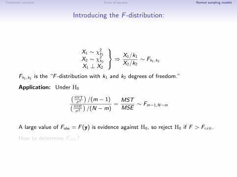

Treatment variation Sums of squares Normal sampling models
Level-α testing procedure
1. gather data
2. construct ANOVA table
3. reject “H0 : µi = µ for all i” if F > Fcrit
where Fcrit is the 1− α quantile of an Ft−1,N−t distribution,
available in R via qf(1−alpha, dof. trt , dof . err ) .
Under this procedure (and a host of assumptions),
Pr(reject H0|H0 true) =
α

Treatment variation Sums of squares Normal sampling models
Level-α testing procedure
1. gather data
2. construct ANOVA table
3. reject “H0 : µi = µ for all i” if F > Fcrit
where Fcrit is the 1− α quantile of an Ft−1,N−t distribution,
available in R via qf(1−alpha, dof. trt , dof . err ) .
Under this procedure (and a host of assumptions),
Pr(reject H0|H0 true) = α

Treatment variation Sums of squares Normal sampling models
Some F distributions
0 5 10 15 20
0.0
0.2
0.4
0.6
F
dens
ity
F(3,20)F(3,10)F(3,5)F(3,2)
0 5 10 15 20
0.2
0.4
0.6
0.8
1.0
F
CD
F
F(3,20)F(3,10)F(3,5)F(3,2)
Try to understand the relationship between curve shape and degrees of freedom.

Treatment variation Sums of squares Normal sampling models
Implementation in R
> anova ( lm ( c t i m e ˜ d i e t ) )A n a l y s i s o f V a r i a n c e Table
Response : c t i m eDf Sum Sq Mean Sq F v a l u e Pr(>F )
d i e t 3 2 2 8 . 0 7 6 . 0 13 .571 4 . 6 5 8 e−05 ∗∗∗R e s i d u a l s 20 1 1 2 . 0 5 . 6
Fobs<−anova ( lm ( c t i m e ˜ d i e t ) ) $F [ 1 ]Fsim<−NULLf o r ( nsim i n 1 : 1 0 0 0 ) {d i e t . sim<−sample ( d i e t )Fsim<−c ( Fsim , anova ( lm ( c t i m e ˜ d i e t . s im ) ) $F [ 1 ] )
}
> mean ( Fsim>=Fobs )[ 1 ] 0
> 1−p f ( Fobs , 3 , 2 0 )[ 1 ] 4 .658471 e−05

Treatment variation Sums of squares Normal sampling models
Null distributions
F
p((F
3,, 2
0))
0 2 4 6 8
0.0
0.2
0.4
0.6
randomization 95th percentilenormal theory 95th percentile

Treatment variation Sums of squares Normal sampling models
Parameter estimates and treatment comparisons
Rejecting H0 indicates evidence that some population means are different.
We can explore this further by making treatment comparisons.
If H0 is rejected we
• estimate µi with yi
• estimate σ2i with
s2i : if sample var are very unequal, this might be a better estimate.
s2p = MSE : if sample var are close and ni is small, this is generally a better
estimate.
Standard practice: Unless there is strong evidence to the contrary, we typically
• assume Var[Yij ] = Var[Ykl ] = σ2,
• and use s2 ≡ MSE to estimate σ2.
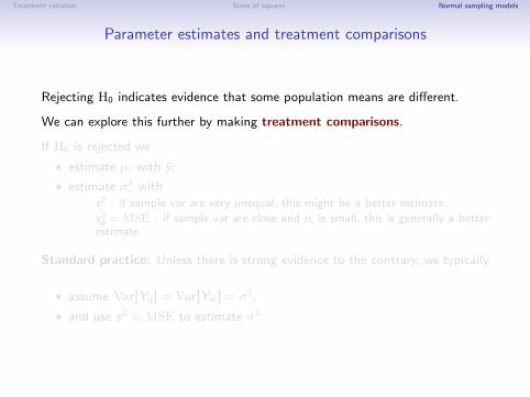
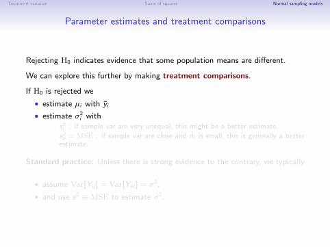

Treatment variation Sums of squares Normal sampling models
Standard error
Assuming equal variances,
Var[µi ] = Var[Yi·] = σ2/ni
≈ s2/ni
The “standard error of the mean” = SE[µi ] =p
s2/ni ,
is an estimate of SD[µi ] =q
Var[Yi·] = σ/√
ni .
The standard error is a very useful quantity.
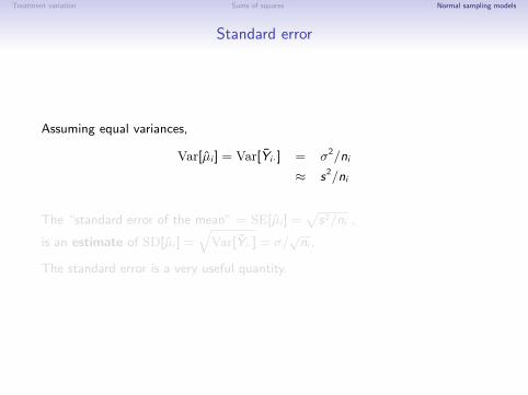
Treatment variation Sums of squares Normal sampling models
Standard error
Assuming equal variances,
Var[µi ] = Var[Yi·] = σ2/ni
≈ s2/ni
The “standard error of the mean” = SE[µi ] =p
s2/ni ,
is an estimate of SD[µi ] =q
Var[Yi·] = σ/√
ni .
The standard error is a very useful quantity.

Treatment variation Sums of squares Normal sampling models
Standard error
Assuming equal variances,
Var[µi ] = Var[Yi·] = σ2/ni
≈ s2/ni
The “standard error of the mean” = SE[µi ] =p
s2/ni ,
is an estimate of SD[µi ] =q
Var[Yi·] = σ/√
ni .
The standard error is a very useful quantity.

Treatment variation Sums of squares Normal sampling models
Standard error
Assuming equal variances,
Var[µi ] = Var[Yi·] = σ2/ni
≈ s2/ni
The “standard error of the mean” = SE[µi ] =p
s2/ni ,
is an estimate of SD[µi ] =q
Var[Yi·] = σ/√
ni .
The standard error is a very useful quantity.

Treatment variation Sums of squares Normal sampling models
Standard error
The usual definition of the standard error of an estimator θ of a parameter θ isan estimate of its sampling standard deviation:
θ = θ(Y)
Var[θ] = γ2
Var[θ] = γ2
SE[θ] = γ
where γ2 is an estimate of γ2.
For example,
µi = Yi·
Var[µi ] = σ2/ni
Var[µi ] = σ2/ni = s2/ni
SE[µi ] = s/√
ni

Treatment variation Sums of squares Normal sampling models
Confidence intervals for treatment means:
Obtaining confidence intervals is very similar to the one-sample case.The only difference is that we use data from all of the groups to estimate thevariance.As a result, the degrees of freedom changes.
Yi· − µi
SE[Yi·]=
Yi· − µipMSE/ni
=Yi· − µi
s/√
ni
∼ tN−m
Note that degrees of freedom are those associated with MSE, NOT ni − 1.As a result,
Yi ± SE[Yi·]× t1−α/2,N−m
is a 100× (1− α)% confidence interval for µi .
A handy rule of thumb:If θ is an estimator of θ, then in many situations
θ ± 2× SE[θ]
is an approximate 95% CI for θ.

Treatment variation Sums of squares Normal sampling models
Coagulation Example
Yi ± SE[Yi·]× t1−α/2,N−m
For 95% confidence intervals,
• t1−α,N−m = t.975,20 = qt (.975,20) ≈ 2.1
• SE[Yi ] =p
s2/ni =p
5.6/ni = 2.37/√
ni
Diet µdiet ni SE[µdiet] 95% CI for µdiet
C 68 6 0.97 (65.9,70.0)B 66 6 0.97 (63.9,68.0)A 61 4 1.18 (58.5,63.5)D 61 8 0.84 (59.2,62.8)

Treatment variation Sums of squares Normal sampling models
Power calculations for the F-testRecall, the power of a test is the probability of rejecting H0 when it is false.Of course, this depends on how the null hypothesis is false.
Power(µ, σ2, n) = Pr(reject H0|µ, σ2, n)
= Pr(Fobs > F1−α,m−1,N−m|µ, σ2, n)
The noncentral F-distribution: Suppose H0 is false , with
Y11 . . . ,Y1n ∼ i.i.d. normal(µ1, σ2)
......
...
Ym1 . . . ,Ymn ∼ i.i.d. normal(µm, σ2)
Under this model, F = F (Y) has a non-central F distribution, with
• degrees of freedom m − 1,N −m
• noncentrality parameter λ
λ = nX
τ 2i /σ
2
where τi = µi − µ is the ith treatment effect.

Treatment variation Sums of squares Normal sampling models
Power
We can gain some more intuition by rewriting λ as follows:
λ = nX
τ 2i /σ
2
= n ×m ׄP
τ 2i
m
«1
σ2
= N × between-treatment variation
within-treatment variation
So power is increasing in N and λ.
Power(µ, σ2, n) = Pr(reject H0|µ, σ2, n)
= Pr(Fobs > F1−α,m−1,N−m|µ, σ2, n)
= 1−pf( qf(1−alpha,m−1,N−m) , m−1 , N−m , ncp=lambda )

Treatment variation Sums of squares Normal sampling models
Power
In many texts, power is expressed as a function of the quantity Φ:
Φ =
rnPτ 2i
σ2m=
sPτ 2i /m
σ2/n=pλ/m
Lets try to understand what Φ represents:
Φ2 =
Pτ 2i /m
σ2/n
=treatment variation
experimental uncertainty
= treatment variation× experimental precision
“treatment variation” means “average squared treatment effect size”.“experimental precision” means “average squared treatment effect size”.

Treatment variation Sums of squares Normal sampling models
Power
2 4 6 8 10
3.0
3.5
4.0
n
F.c
rit
2 4 6 8 1010
1520
2530
3540
nλλ
2 4 6 8 10
0.4
0.6
0.8
1.0
n
pow
er
m == 4 αα == 0.05 var.b/var.w=1
2 4 6 8 10
3.0
3.5
4.0
n
F.c
rit
2 4 6 8 10
2030
4050
6070
80
n
λλ
2 4 6 8 100.
750.
850.
95n
pow
er
m == 4 αα == 0.05 var.b/var.w=2