Embed Size (px)
Citation preview
Introduction to Analog And Digital Communications
Second Edition
Simon Haykin, Michael Moher
Chapter 9 Noise in Analog Communications
9.1 Noise in Communication Systems9.2 Signal-to-Noise Ratios9.3 Band-Pass Receiver Structures9.4 Noise in Linear Receivers Using Coherent Detection9.5 Noise in AM Receivers Using Envelope Detection9.6 Noise in SSB Receivers9.7 Detection of Frequency Modulation (FM)9.8 FM Pre-emphasis and De-emphasis9.9 Summary and Discussion
3
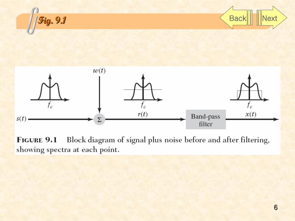
Noise can broadly be defined as any unknown signal that affects the recovery of the desired signal.
The received signal is modeled as
is the transmitted signal
is the additive noise
)1.9()()()( twtstr +=
)(ts
)(tw
4
Lesson 1 : Minimizing the effects of noese is a prime concern in analog communications, and consequently the ratio of signal power is an important metric for assessing analog communication quality.
Lesson 2 : Amplitude modulation may be detected either coherently requiring the use of a synchronized oscillator or non-coherently by means of a simple envelope detector. However, there is a performance penalty to be paid for non-coherent detection.
Lesson 3 : Frequency modulation is nonlinear and the output noise spectrum is parabolic when the input noise spectrum is flat. Frequency modulation has the advantage that it allows us to trade bandwidth for improved performance.
Lesson 4 : Pre-and de-emphasis filtering is a method of reducing the output noise of an FM demodulator without distorting the signal. This technique may be used to significantly improve the performance of frequency modulation systims.
5
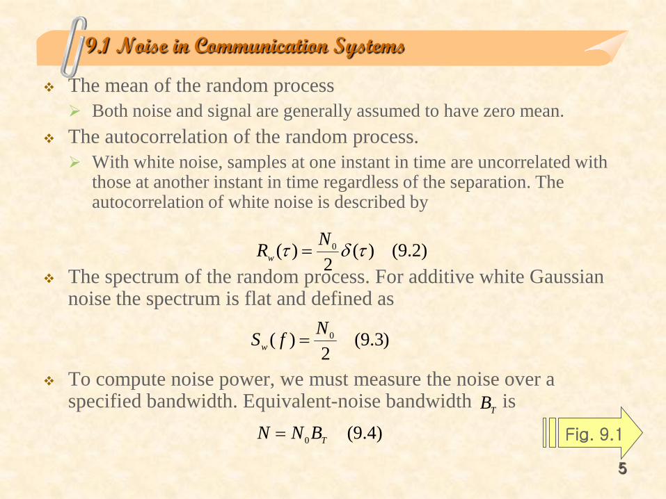
9.1 Noise in Communication Systems
The mean of the random process Both noise and signal are generally assumed to have zero mean.
The autocorrelation of the random process. With white noise, samples at one instant in time are uncorrelated with
those at another instant in time regardless of the separation. The autocorrelation of white noise is described by
The spectrum of the random process. For additive white Gaussian noise the spectrum is flat and defined as
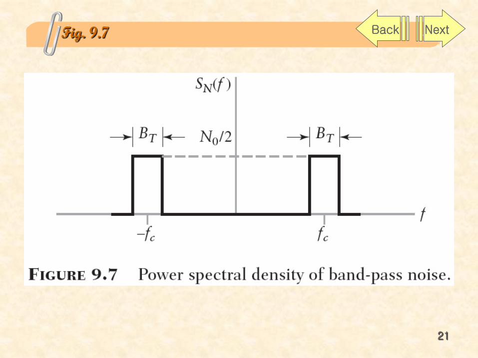
To compute noise power, we must measure the noise over a specified bandwidth. Equivalent-noise bandwidth is
)2.9()(2
)( 0 τδτ NRw =
)3.9(2
)( 0NfSw =
)4.9(0 TBNN = Fig. 9.1
TB
6
Fig. 9.1 Back Next
7
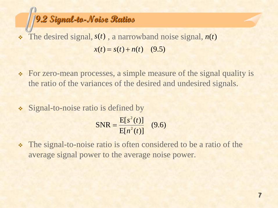
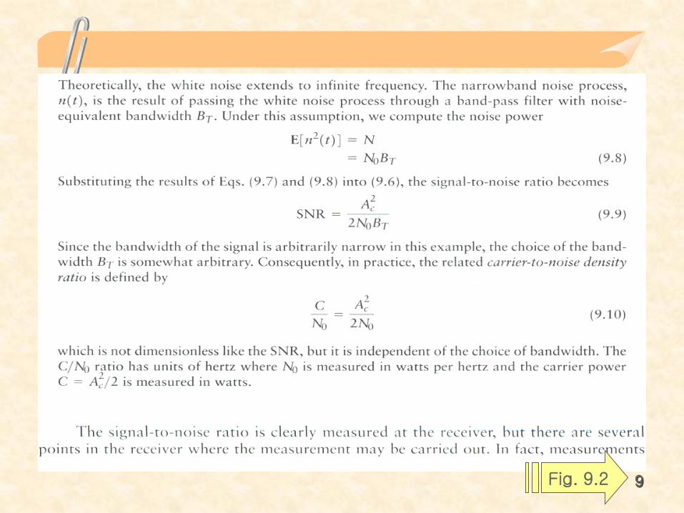
9.2 Signal-to-Noise Ratios
The desired signal, , a narrowband noise signal,
For zero-mean processes, a simple measure of the signal quality is the ratio of the variances of the desired and undesired signals.
Signal-to-noise ratio is defined by
The signal-to-noise ratio is often considered to be a ratio of the average signal power to the average noise power.
)5.9()()()( tntstx +=
)6.9()]([E)]([ESNR 2
2
tnts
=
)(ts )(tn
8
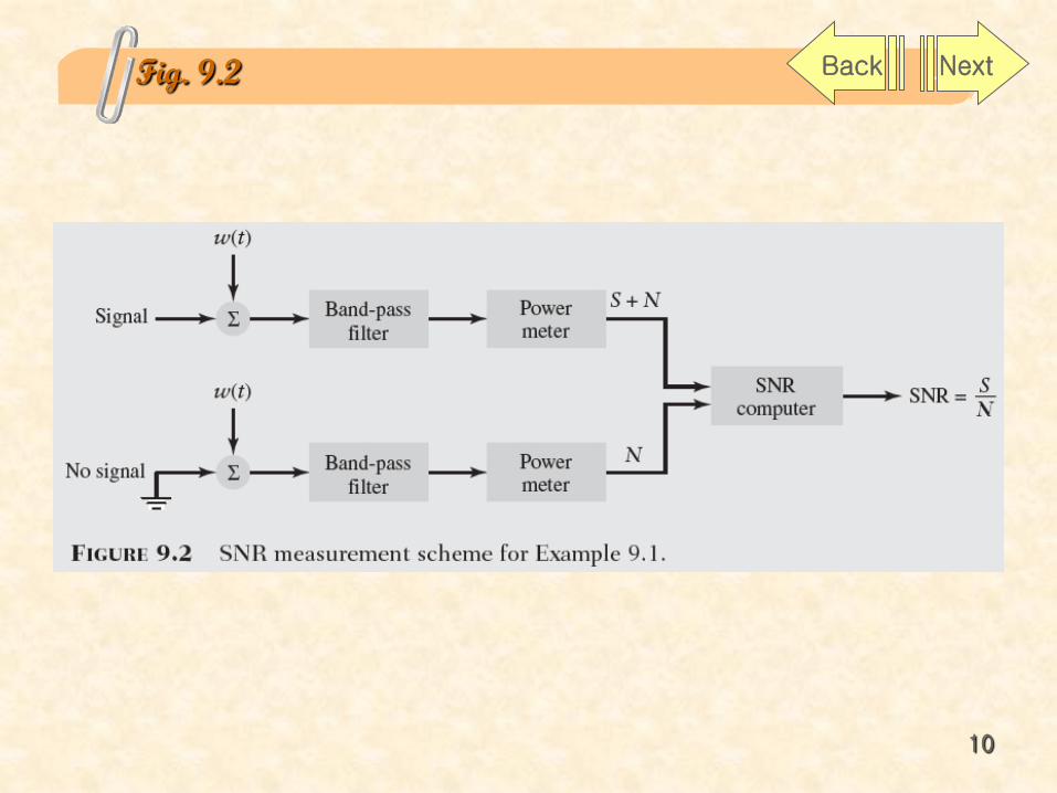
9Fig. 9.2
10
Fig. 9.2 Back Next
11
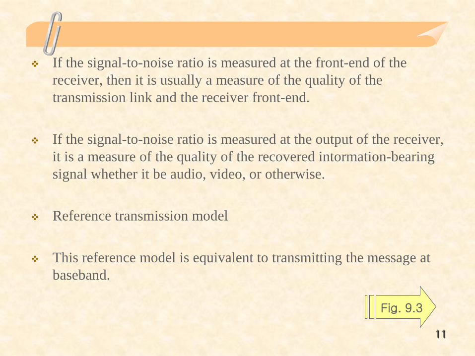
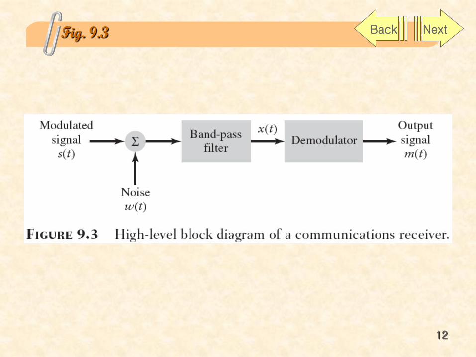
If the signal-to-noise ratio is measured at the front-end of the receiver, then it is usually a measure of the quality of the transmission link and the receiver front-end.
If the signal-to-noise ratio is measured at the output of the receiver, it is a measure of the quality of the recovered intormation-bearing signal whether it be audio, video, or otherwise.
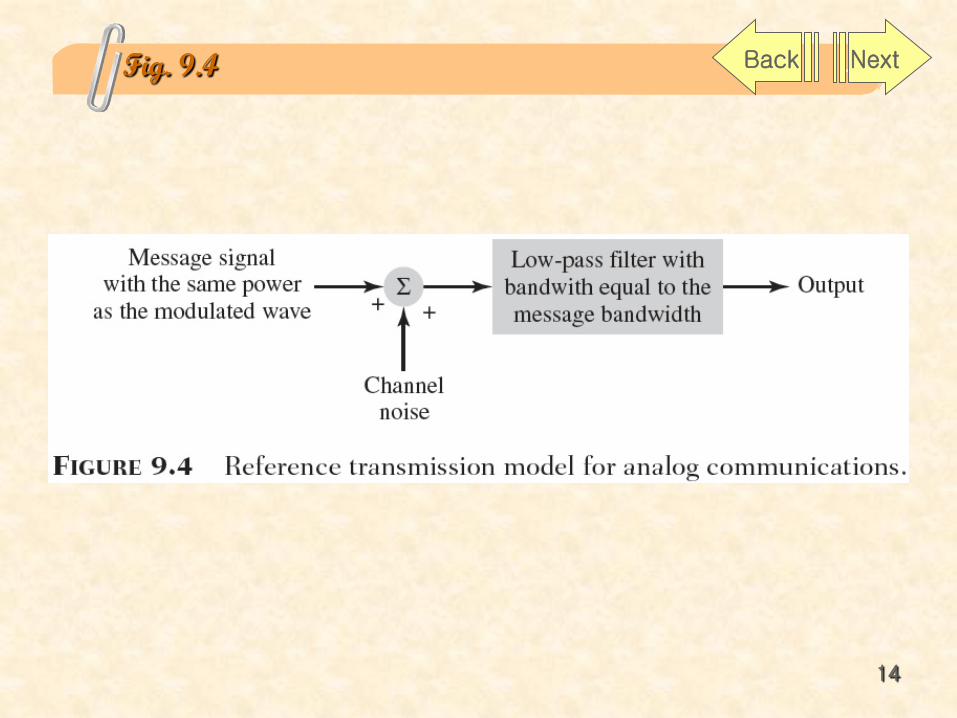
Reference transmission model
This reference model is equivalent to transmitting the message at baseband.
Fig. 9.3
12
Fig. 9.3 Back Next
13
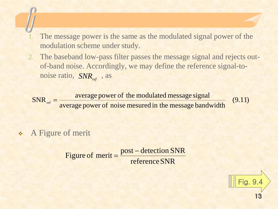
1. The message power is the same as the modulated signal power of the modulation scheme under study.
2. The baseband low-pass filter passes the message signal and rejects out-of-band noise. Accordingly, we may define the reference signal-to-noise ratio, , as
A Figure of merit
refSNR
)11.9(bandwidth message in the mesured noise ofpower average
signal message modulated theofpower averageSNR ref =
SNR referenceSNRdetection postmerit of Figure −
=
Fig. 9.4
14
Fig. 9.4 Back Next
15
The higher the value that the figure of merit gas, the better the noise performance of the receiver will be.
To summarize our consideration of signal-to-noise ratios: The pre-detection SNR is measured before the signal is demodulated. The post-detection SNR is measured after the signal is demodulated. The reference SNR is defined on the basis of a baseband transmission
model. The figure of merit is a dimensionless metric for comparing sifferent
analog modulation-demodulation schemes and is defined as the ratio of the post-detection and reference SNRs.
16
9.3 Band-Pass Receiver Structures
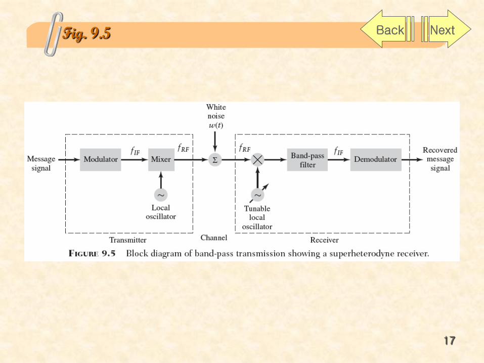
Fig. 9.5 shows an example of a superheterodyne receiver AM radio transmissions Common examples are AM radio transmissions, where the RF channels’
frequencies lie in the range between 510 and 1600 kHz, and a common IF is 455 kHz
FM radio Another example is FM radio, where the RF channels are in the range from 88
to 108 MHz and the IF is typically 10.7 MHz.
The filter preceding the local oscillator is centered at a higher RF frequency and is usually much wider, wide enough to encompass all RF channels that the receiver is intended to handle.
With the same FM receiver, the band-pass filter after the local oscillator would be approximately 200kHz wide; it is the effects of this narrower filter that are of most interest to us.
)12.9()2sin()()2cos()()( tftstftsts cQcI ππ −=
Fig. 9.5
17
Fig. 9.5 Back Next
18
9.4 Noise in Linear Receivers Using Coherent Detection
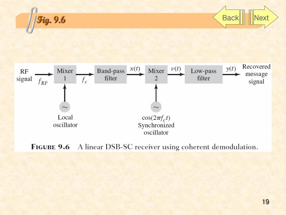
Double-sideband suppressed-carrier (DSB-SC) modulation, the modulated signal is represented as
is the carrier frequency is the message signal The carrier phase In Fig. 9.6, the received RF signal is the sum of the modulated
signal and white Gaussian noise After band-pass filtering, the resulting signal is
)13.9()2cos()()( θπ += tftmAts cc
)14.9()()()( tntstx +=
cf
)(tm
θ
)(tw
Fig. 9.6
19
Fig. 9.6 Back Next
20
In Fig.9.7 The assumed power spectral density of the band-pass noise is illustrated
For the signal of Eq. (9.13), the average power of the signal component is given by expected value of the squared magnitude.
The carrier and modulating signal are independent
Pre-detection signal-to-noise ratio of the DSB-SC system A noise bandwidth The signal-to-noise ratio of the signal is
)15.9()]([E]))2cos([(E)]([E 222 tmtfAts cc θπ +=
)16.9()]([E 2 tmP =
)17.9(2
)]([E2
2 PAts c=
)18.9(2
SNR0
2DSBpre
T
c
BNPA
=
)(ts
TB
Fig. 9.7
21
Fig. 9.7 Back Next
22
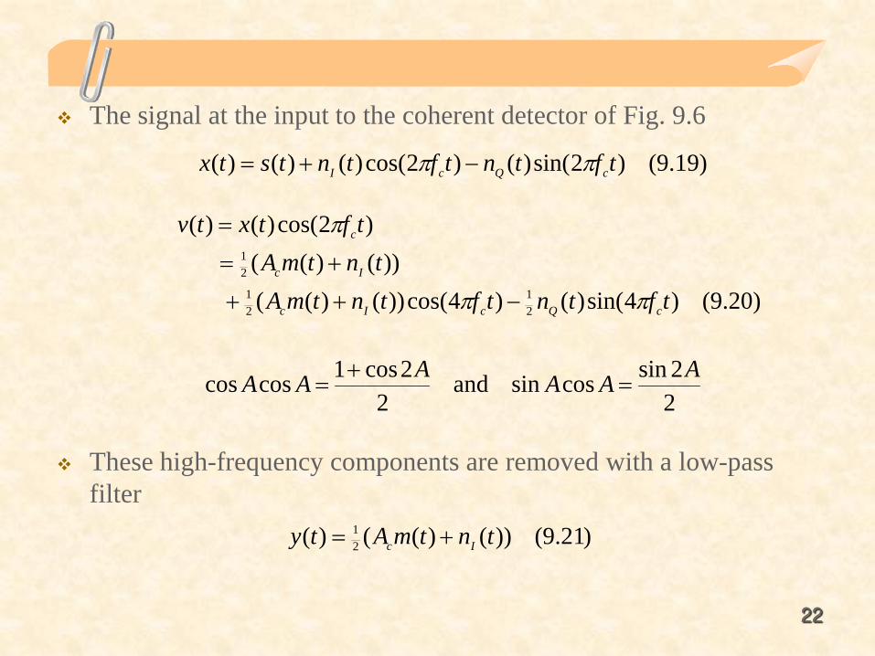
The signal at the input to the coherent detector of Fig. 9.6
These high-frequency components are removed with a low-pass filter
)19.9()2sin()()2cos()()()( tftntftntstx cQcI ππ −+=
)20.9()4sin()()4cos())()(( ))()((
)2cos()()(
21
21
21
tftntftntmAtntmA
tftxtv
cQcIc
Ic
c
ππ
π
−++
+=
=
22sincossinand
22cos1coscos AAAAAA =
+=
)21.9())()(()( 21 tntmAty Ic +=
23
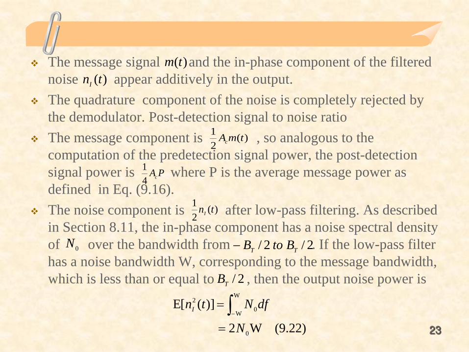
The message signal and the in-phase component of the filtered noise appear additively in the output.
The quadrature component of the noise is completely rejected by the demodulator. Post-detection signal to noise ratio
The message component is , so analogous to the computation of the predetection signal power, the post-detection signal power is where P is the average message power as defined in Eq. (9.16).
The noise component is after low-pass filtering. As described in Section 8.11, the in-phase component has a noise spectral density of over the bandwidth from . If the low-pass filter has a noise bandwidth W, corresponding to the message bandwidth, which is less than or equal to , then the output noise power is
)22.9(W2
)]([E
0
W
W 02
N
dfNtnI
=
= ∫−
)(tm)(tnI
)(21 tmAc
PAc41
)(21 tnI
0N 2/2/ TT BtoB−
2/TB
24
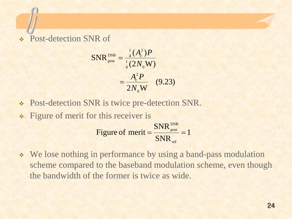
Post-detection SNR of
Post-detection SNR is twice pre-detection SNR. Figure of merit for this receiver is
We lose nothing in performance by using a band-pass modulation scheme compared to the baseband modulation scheme, even though the bandwidth of the former is twice as wide.
)23.9(W2
)W2()(SNR
0
2
041
241
DSBpost
NPA
NPA
c
c
=
=
1SNRSNR
merit of Figureref
DSBpost ==
25
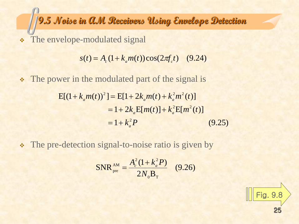
9.5 Noise in AM Receivers Using Envelope Detection
The envelope-modulated signal
The power in the modulated part of the signal is
The pre-detection signal-to-noise ratio is given by
)24.9()2cos())(1()( tftmkAts cac π+=
)25.9( 1 )]([E)]([E21
)]()(21[E]))(1[(E
2
22
222
Pktmktmk
tmktmktmk
a
aa
aaa
+=
++=
++=+
Fig. 9.8
)26.9(B2
)1(SNRT0
22AMpre N
PkA ac +=
26
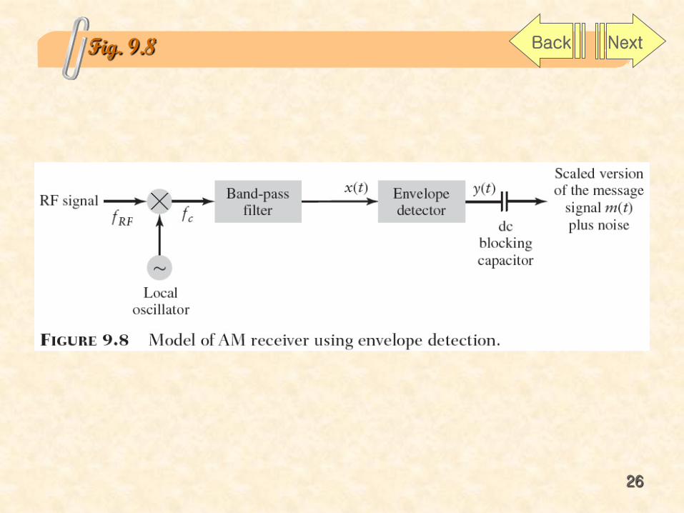
Fig. 9.8 Back Next
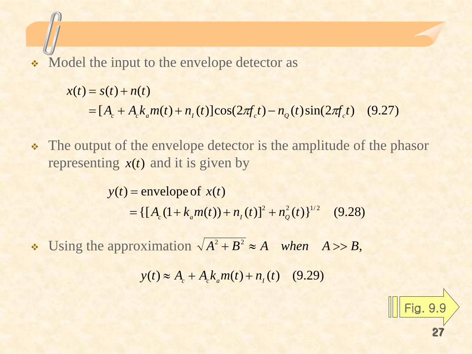
27
Model the input to the envelope detector as
The output of the envelope detector is the amplitude of the phasor representing and it is given by
Using the approximation
)27.9()2sin()()2cos()]()([ )()()(
tftntftntmkAAtntstx
cQcIacc ππ −++=+=
)28.9()}()]())(1({[ )( of envelope)(
2/122 tntntmkAtxty
QIac +++=
=
)29.9()()()( tntmkAAty Iacc ++≈
Fig. 9.9
)(tx
,22 BAwhenABA >>≈+
28
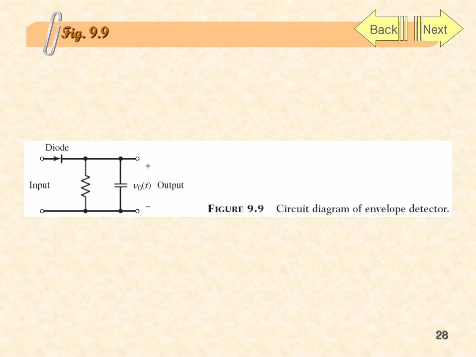
Fig. 9.9 Back Next
29
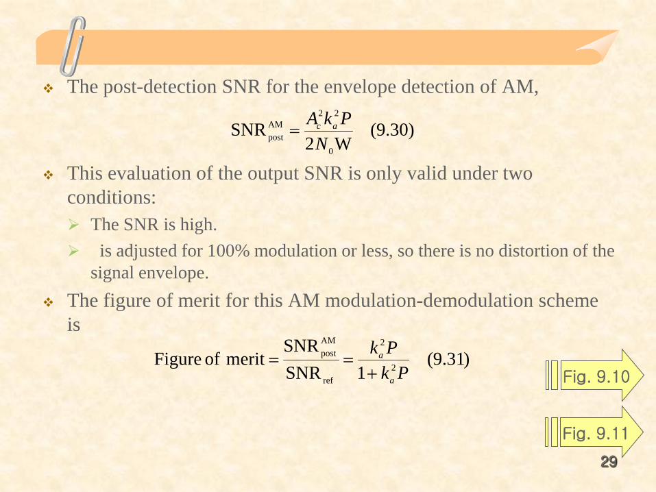
The post-detection SNR for the envelope detection of AM,
This evaluation of the output SNR is only valid under two conditions: The SNR is high. is adjusted for 100% modulation or less, so there is no distortion of the
signal envelope. The figure of merit for this AM modulation-demodulation scheme
is
)30.9(W2
SNR0
22AMpost N
PkA ac=
)31.9(1SNR
SNRmerit of Figure 2
2
ref
AMpost
PkPka
a
+==
Fig. 9.10
Fig. 9.11
30
Fig. 9.10 Back Next
31
Fig. 9.11 Back Next
32
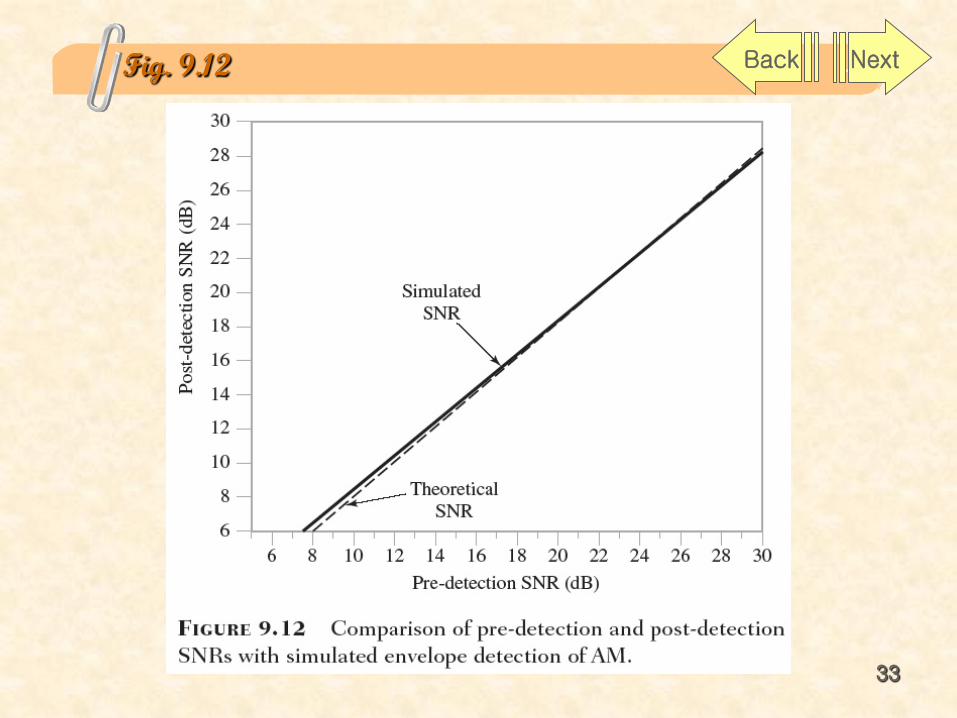
In the experiment, the message is a sinusoidal wave We compute the pre-detection and post-detection SNRs for samples of its
signal. These two measures are plotted against one another in Fig. 9.12 for.
The post-detection SNR is computed as follows: The output signal power is determined by passing a noiseless signal through the
envelope detector and measuring the output power. The output noise is computed by passing plus noise through the envelope
detector and subtracting the output obtained form the clean signal only. With this approach, any distortion due to the product of noise and signal components is included as noise contribution.
From Fig.9.12, there is close agreement between theory and experiment at high SNR values, which is to be expected. There are some minor discrepancies, but these can be attributed to the limitations of the discrete time simulation. At lower SNR there is some variation from theory as might also be expected.
Fig. 9.12
),2sin()( tfAtm mπ=
3.0=ak
33
Fig. 9.12 Back Next
34
9.6 Noise in SSB Receivers
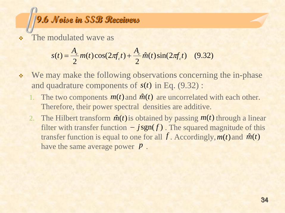
The modulated wave as
We may make the following observations concerning the in-phase and quadrature components of in Eq. (9.32) :
1. The two components and are uncorrelated with each other. Therefore, their power spectral densities are additive.
2. The Hilbert transform is obtained by passing through a linear filter with transfer function . The squared magnitude of this transfer function is equal to one for all . Accordingly, and have the same average power .
)32.9()2sin()(ˆ2
)2cos()(2
)( tftmAtftmAts cc
cc ππ +=
)(ts)(tm )(ˆ tm
)(ˆ tm )(tm)sgn( fj−
fp
)(tm )(ˆ tm
35
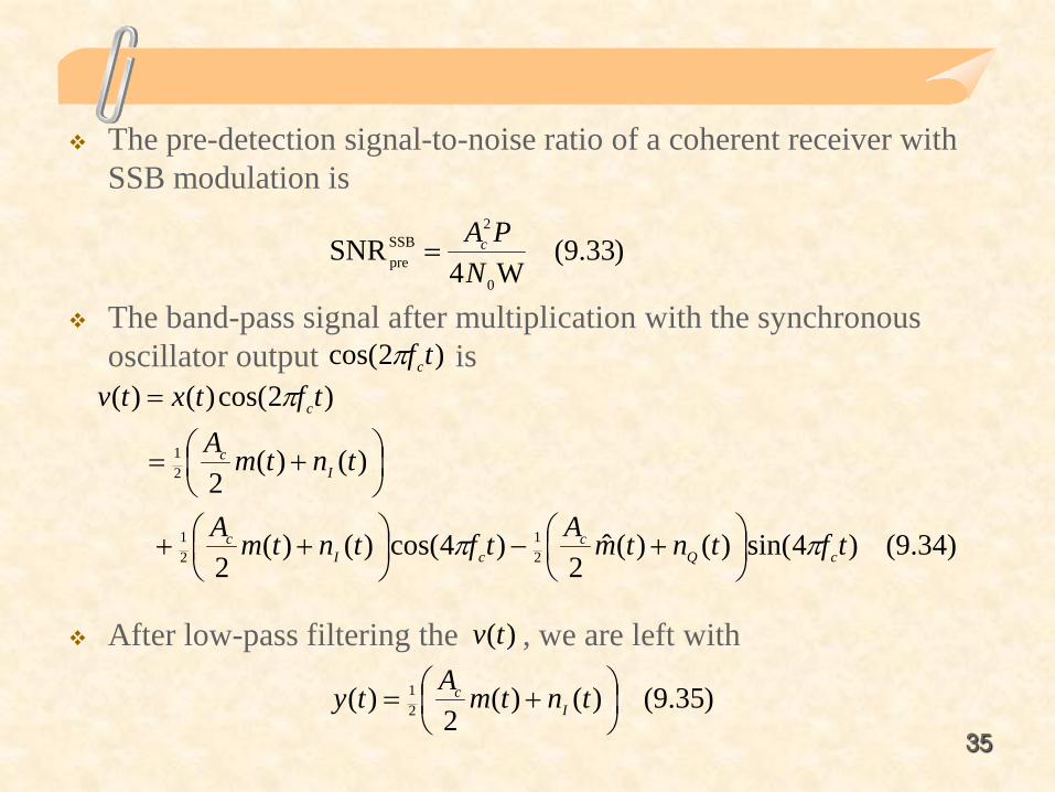
The pre-detection signal-to-noise ratio of a coherent receiver with SSB modulation is
The band-pass signal after multiplication with the synchronous oscillator output is
After low-pass filtering the , we are left with
)33.9(W4
SNR0
2SSBpre N
PAc=
)34.9()4sin()()(ˆ2
)4cos()()(2
)()(2
)2cos()()(
21
21
21
tftntmAtftntmA
tntmAtftxtv
cQc
cIc
Ic
c
ππ
π
+−
++
+=
=
)35.9()()(2
)( 21
+= tntmAty I
c
)(tv
)2cos( tfcπ
36
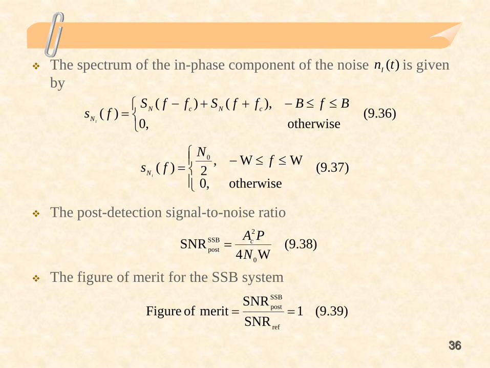
The spectrum of the in-phase component of the noise is given by
The post-detection signal-to-noise ratio
The figure of merit for the SSB system
)36.9( otherwise ,0
),()()(
≤≤−++−
=BfBffSffS
fs cNcNN I
)37.9( otherwise ,0
WW,2)(
0
≤≤−= fN
fsIN
)38.9(W4
SNR0
2SSBpost N
PAc=
)39.9(1SNRSNR
merit of Figureref
SSBpost ==
)(tnI
37
Comparing the results for the different amplitude modulation schemes There are a number of design tradeoffs.
Single-sideband modulation achieves the same SNR performance as the baseband reference model but only requires half the transmission bandwidth of the DSC-SC system.
SSB requires more transmitter processing.
38
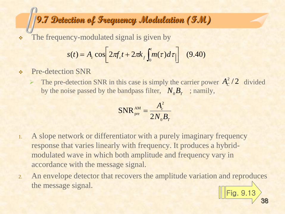
9.7 Detection of Frequency Modulation (FM)
The frequency-modulated signal is given by
Pre-detection SNR The pre-detection SNR in this case is simply the carrier power divided
by the noise passed by the bandpass filter, ; namily,
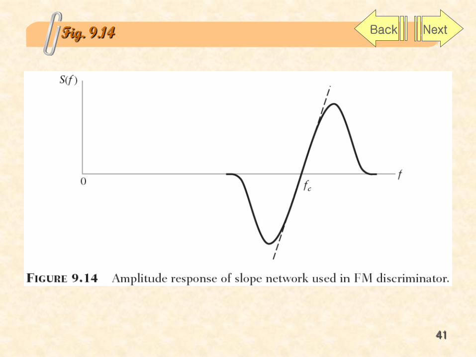
1. A slope network or differentiator with a purely imaginary frequency response that varies linearly with frequency. It produces a hybrid-modulated wave in which both amplitude and frequency vary in accordance with the message signal.
2. An envelope detector that recovers the amplitude variation and reproduces the message signal.
)40.9()(22cos)(0
+= ∫
t
fcc dmktfAts ττππ
2/2CA
TBN0
T
c
BNA
0
2AMpre 2
SNR =
Fig. 9.13
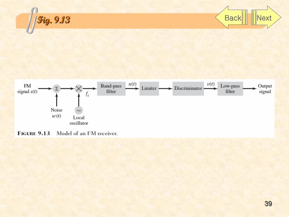
39
Fig. 9.13 Back Next
40
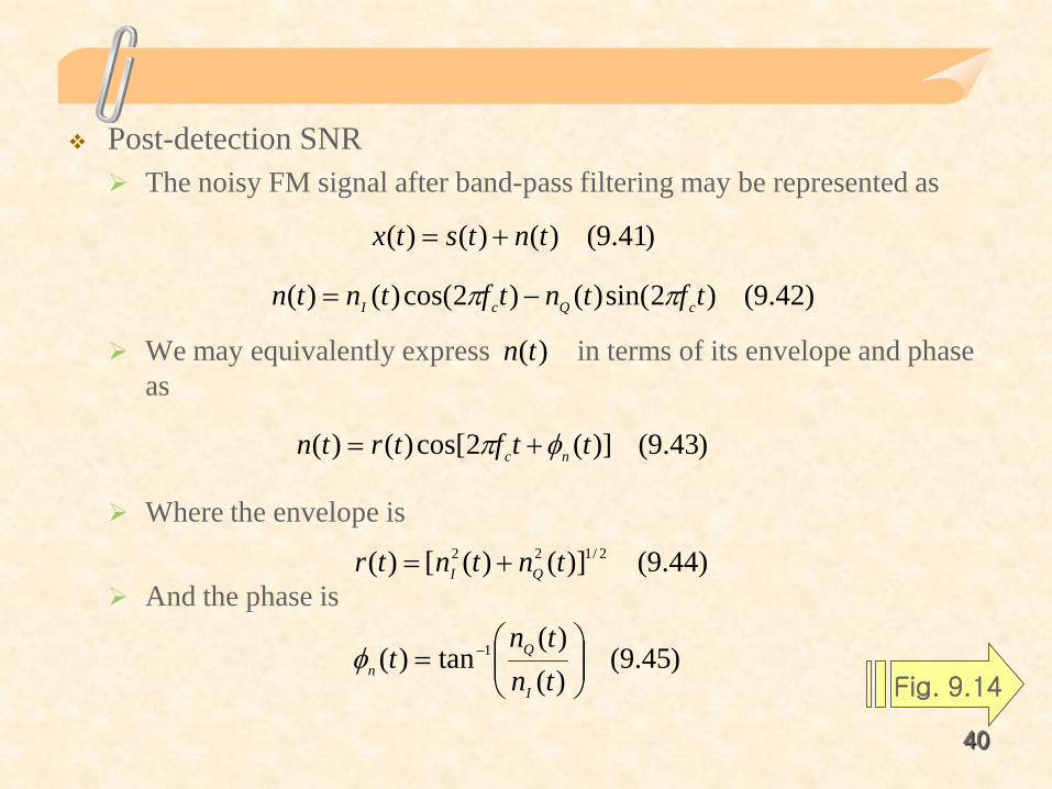
Post-detection SNR The noisy FM signal after band-pass filtering may be represented as
We may equivalently express in terms of its envelope and phase as
Where the envelope is
And the phase is
)41.9()()()( tntstx +=
)42.9()2sin()()2cos()()( tftntftntn cQcI ππ −=
)43.9()](2cos[)()( ttftrtn nc φπ +=
)(tn
)44.9()]()([)( 2/122 tntntr QI +=
)45.9()()(
tan)( 1
= −
tntn
tI
Qnφ
Fig. 9.14
41
Fig. 9.14 Back Next
42
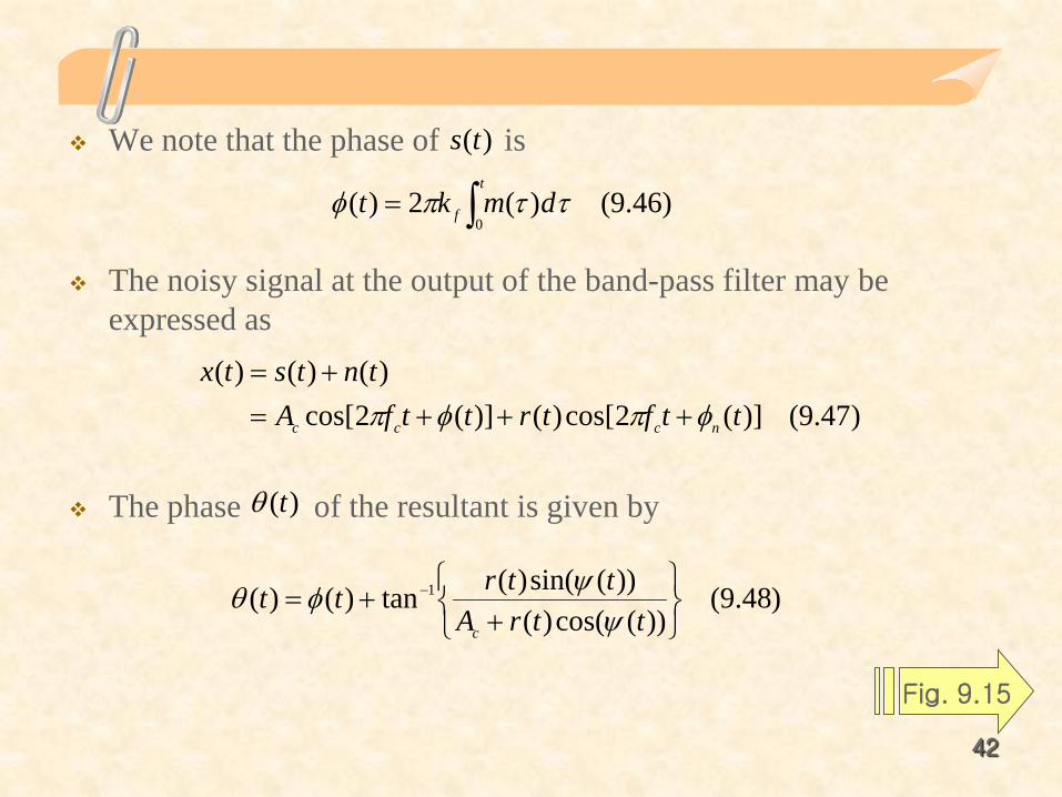
We note that the phase of is
The noisy signal at the output of the band-pass filter may be expressed as
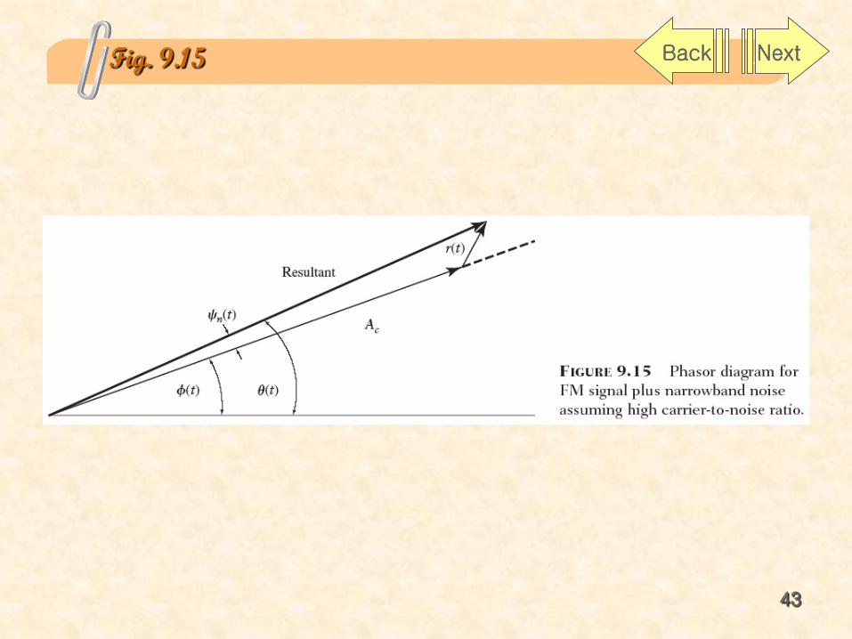
The phase of the resultant is given by
)46.9()(2)(0∫=t
f dmkt ττπφ
)47.9()](2cos[)()](2cos[ )()()(
ttftrttfAtntstx
nccc φπφπ +++=+=
)48.9())(cos()(
))(sin()(tan)()( 1
++= −
ttrAttrtt
c ψψφθ
)(ts
)(tθ
Fig. 9.15
43
Fig. 9.15 Back Next
44
Under this condition, and noting that , the expression for the phase simplifies to
Then noting that the quadrature component of the noise iswe may simplify Eq.(9.49) to
The ideal discriminator output
)50.9()(
)()(c
Q
Atn
tt +=φθ
)51.9()(
)(2)(0
c
Qt
f Atn
dmkt +≈ ∫ ττπθ
)52.9()()(
)(21)(
tntmkdt
tdtv
df +=
=θ
π
)49.9()](sin[)()()( tAtrttc
ψφθ +=
1sintan 1 <<≈− ξξξ ce
)],(sin[)()( ttrtn nQ φ=
45
The noise term is defined by
The additive noise at the discriminator output is determined essentially by the quadrature component of the marrowband noise .
The power spectral density of the quadrature noise compinentas follows;
)53.9()(
21)(
dttdn
Atn Q
cd π
=
)54.9(22)(
cc Ajf
AfjfG ==
ππ
)55.9()(
)(|)(|)(
2
2
2
fSAf
fSfGfS
Q
Qd
Nc
NN
=
=
)(tnd
)(tnQ
)(tn
)( fSQN
)(tnQ
46
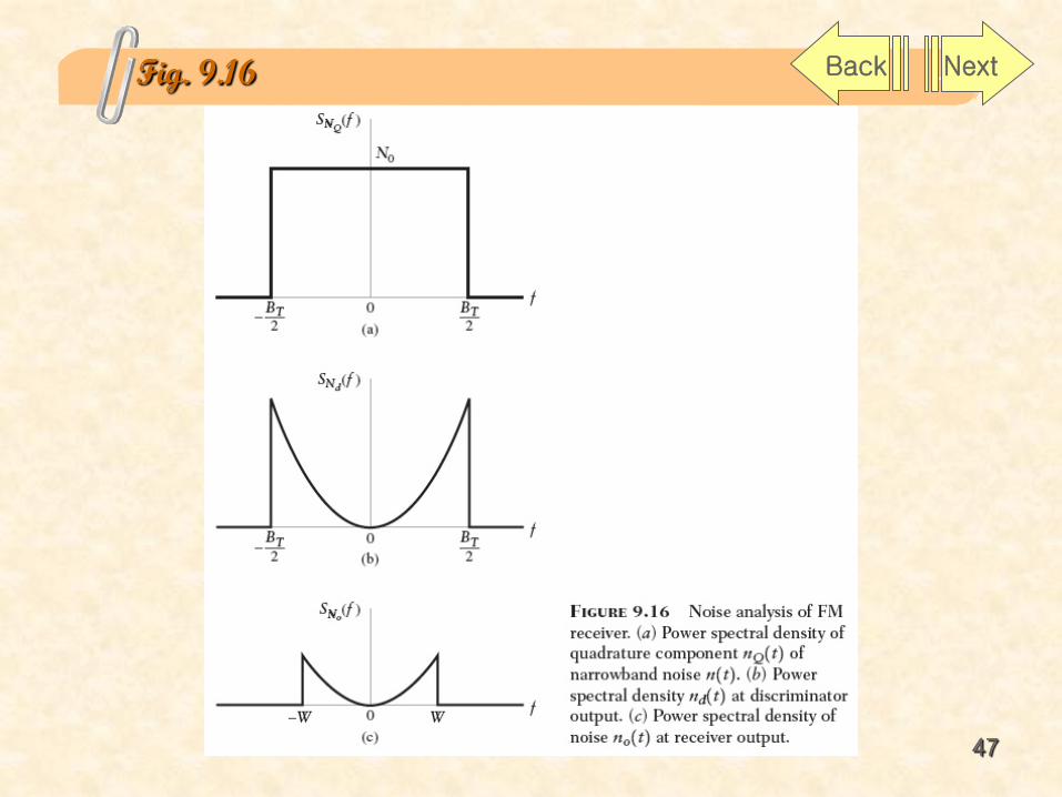
Power spectral density of the noise is shown in Fig.9.16
Therefore, the power spectral density of the noise appearing at the receiver output is defined by
)56.9(otherwise ,0
2||,)( 2
20
<
=T
cN
BfA
fNfS
d
)57.9(otherwise ,0
W||,)( 2
20
0
<
=f
AfN
fScN
)58.9(3
W2
power noisedetection -post Average
2
30
W
W
220
c
c
AN
dffAN
=
= ∫−
)(tnd
Fig. 9.16
)(0
fSN )(0 tn
47
Fig. 9.16 Back Next
48
Figure of merit
The figure of merit for an FM system is approximately given by
)59.9(W2
3SNR 3
0
22FMpost N
PkA fc=
)60.9( 3
W3
W2
W23
SNRSNR
merit of Figure
2
2
2
0
2
30
22
ref
FMpost
D
PkNA
NPkA
f
c
fc
=
=
==
)61.9(W4
3merit of Figure2
≈ TB
49
Thus, when the carrier to noise level is high, unlike an amplitude modulation system an FM system allows us to trade bandwidth for improved performance in accordance with square law.
50
51
52
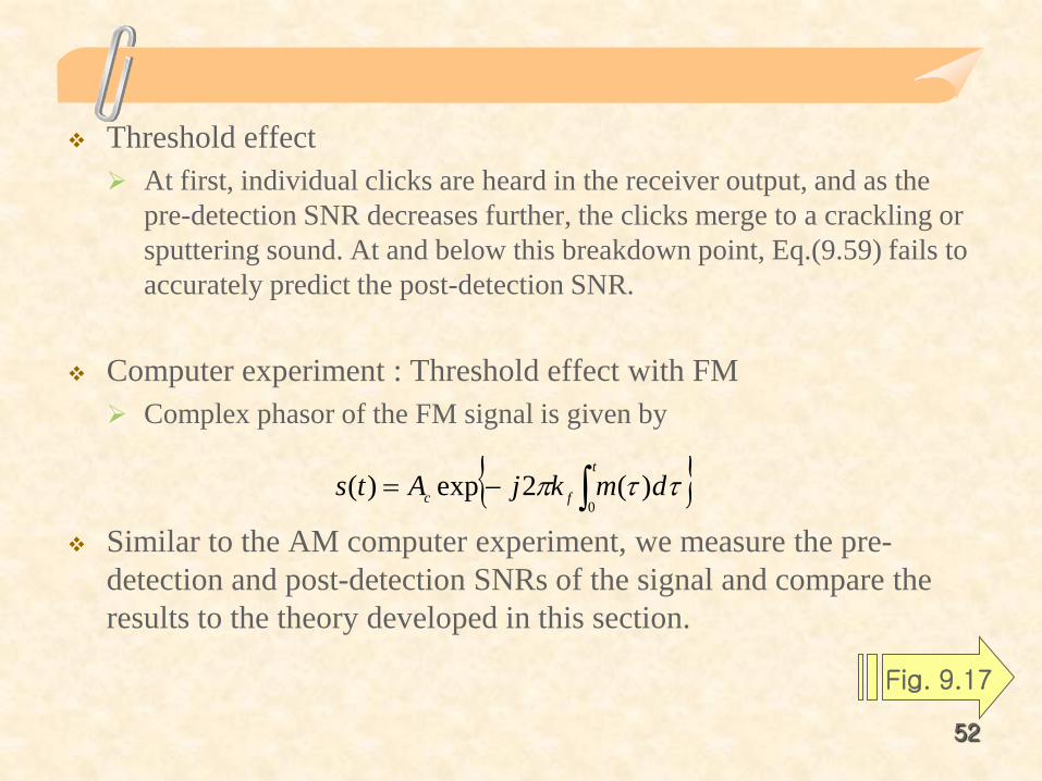
Threshold effect At first, individual clicks are heard in the receiver output, and as the
pre-detection SNR decreases further, the clicks merge to a crackling or sputtering sound. At and below this breakdown point, Eq.(9.59) fails to accurately predict the post-detection SNR.
Computer experiment : Threshold effect with FM Complex phasor of the FM signal is given by
Similar to the AM computer experiment, we measure the pre-detection and post-detection SNRs of the signal and compare the results to the theory developed in this section.
Fig. 9.17
{ }∫−=t
fc dmkjAts0
)(2exp)( ττπ
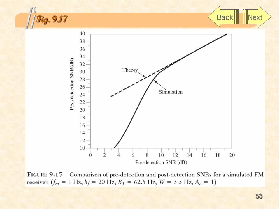
53
Fig. 9.17 Back Next
54
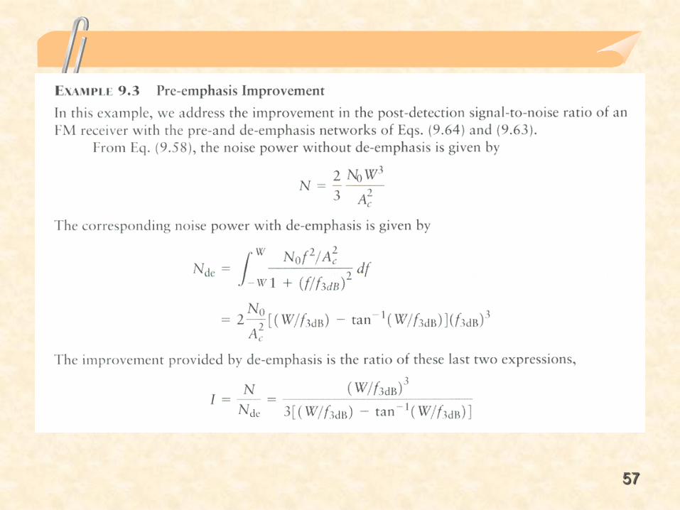
9.8 FM Pre-emphasis and De-emphasis
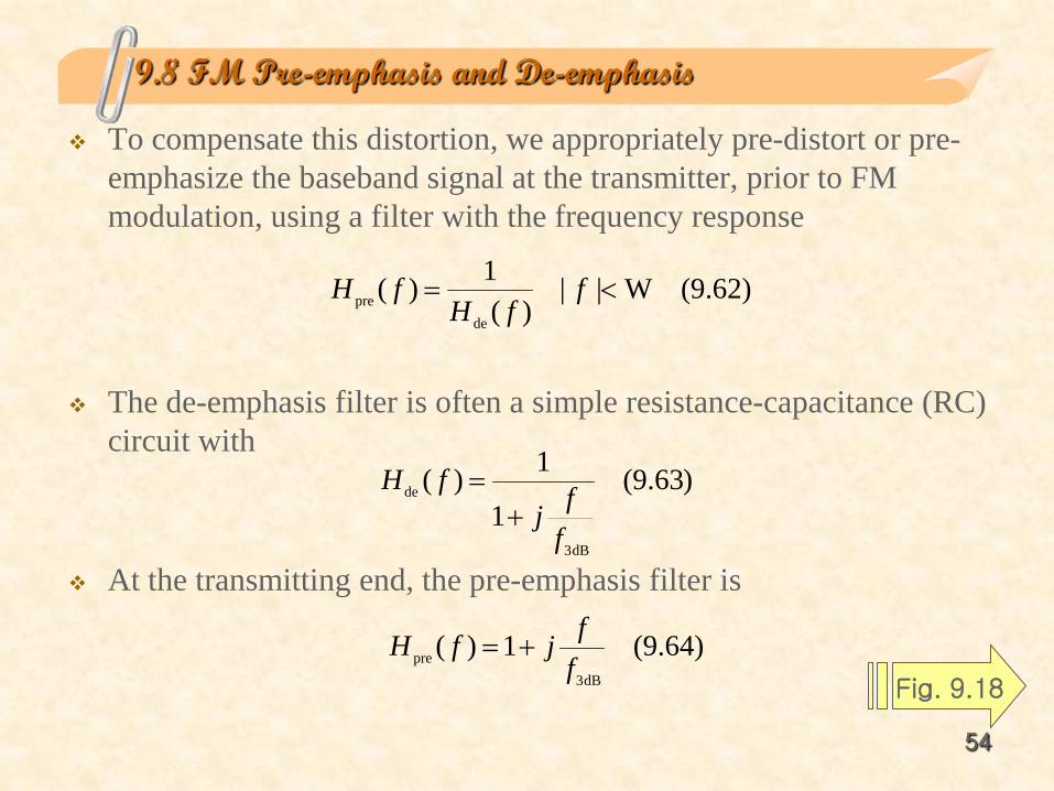
To compensate this distortion, we appropriately pre-distort or pre-emphasize the baseband signal at the transmitter, prior to FM modulation, using a filter with the frequency response
The de-emphasis filter is often a simple resistance-capacitance (RC) circuit with
At the transmitting end, the pre-emphasis filter is
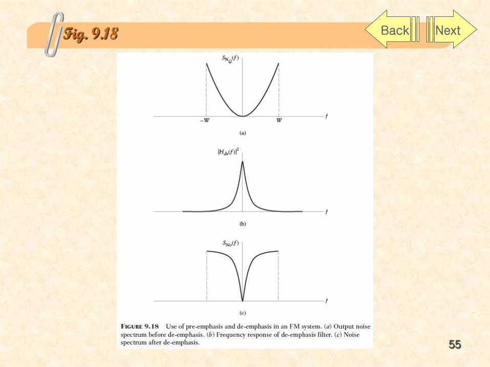
Fig. 9.18
)62.9(W||)(
1)(de
pre <= ffH
fH
)63.9(1
1)(
dB3
de
ffj
fH+
=
)64.9(1)(dB3
pre ffjfH +=
55
Fig. 9.18 Back Next
56
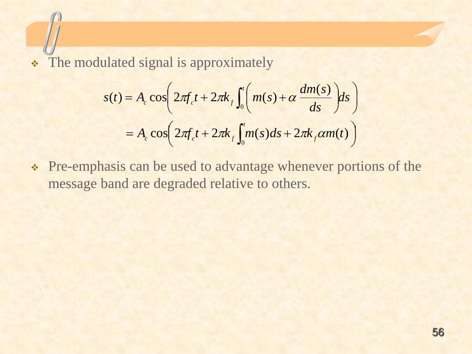
The modulated signal is approximately
Pre-emphasis can be used to advantage whenever portions of the message band are degraded relative to others.
++=
++=
∫
∫)(2)(22cos
)()(22cos)(
0
0
tmkdssmktfA
dsds
sdmsmktfAts
f
t
fcc
t
fcc
απππ
αππ
57
58
9.9 Summary and Discussion
We analyzed the noise performance of a number of different amplitude modulation schemes and found:
1. The detection of DSB-SC with a linear coherent receiver has the same SNR performance as the baseband reference model but requires synchronization circuitry to recover the coherent carrier for demodulation.
2. Non-suppressed carrier AM systems allow simple receiver design including the use of envelope detection, but they result in significant wastage of transmitter power compared to coherent systems.
3. Analog SSB modulation provides the same SNR performance as DSB-SC while requiring only half the transmission bandwidth.
In this chapter, we have shown the importance of noise analysis based on signal-to-noise ratio in the evaluation of the performance of analog communication systems. This type system, be it analog or digital.