DSP2009.doc 1

Introduction to DSP: Text Books : (P) = Proakis , (M) = Mitra (I) = Iffeachor. (previous reference continues to apply unless change is indicated)

Advantages: • Guaranteed accuracy: no. of bits • Perfect reproducibility: no equipment dependence, tolerances etc. • No drift in performance with age, temp, • With CMOS, reliability, small size, low cost, low power and high speed • Flexibility: a given system can be reprogrammed, with same hardware • Superior, near ideal performance: i.e. linearity, adaptive filtering etc • Storage: digital storage media can be used

Classification of Signals: (P,M)

Multichannel and Multidimensional Signal is a function of one or more variables. It can be real valued, complex valued or a vector

• tA π3sin is real valued • tjAe π3 is complex valued

Vector signals are generated by multiple sources. E.g. 3 lead ECG, RGB, and are multichannel signals. The variable may be 1-dimensional e.g. t A picture signal (B&W) is 2-dimensional as it is a function of x and y Colour TV is 3 channel 3 dimensional e.g. (x,y,t),

Continuous Time and Discrete Time Signals: (P,M) • Continuous time signals are defined for all value of time i.e. speech • Discrete time signals defined at specific instances of time x[n]

Continuous time signals may be

• analog if all values are allowed, or • Quantized Boxcar signals if specific values are allowed.

Discrete time signals may be

• digital (specific values) or • sampled (any value)

DSP2009.doc 2

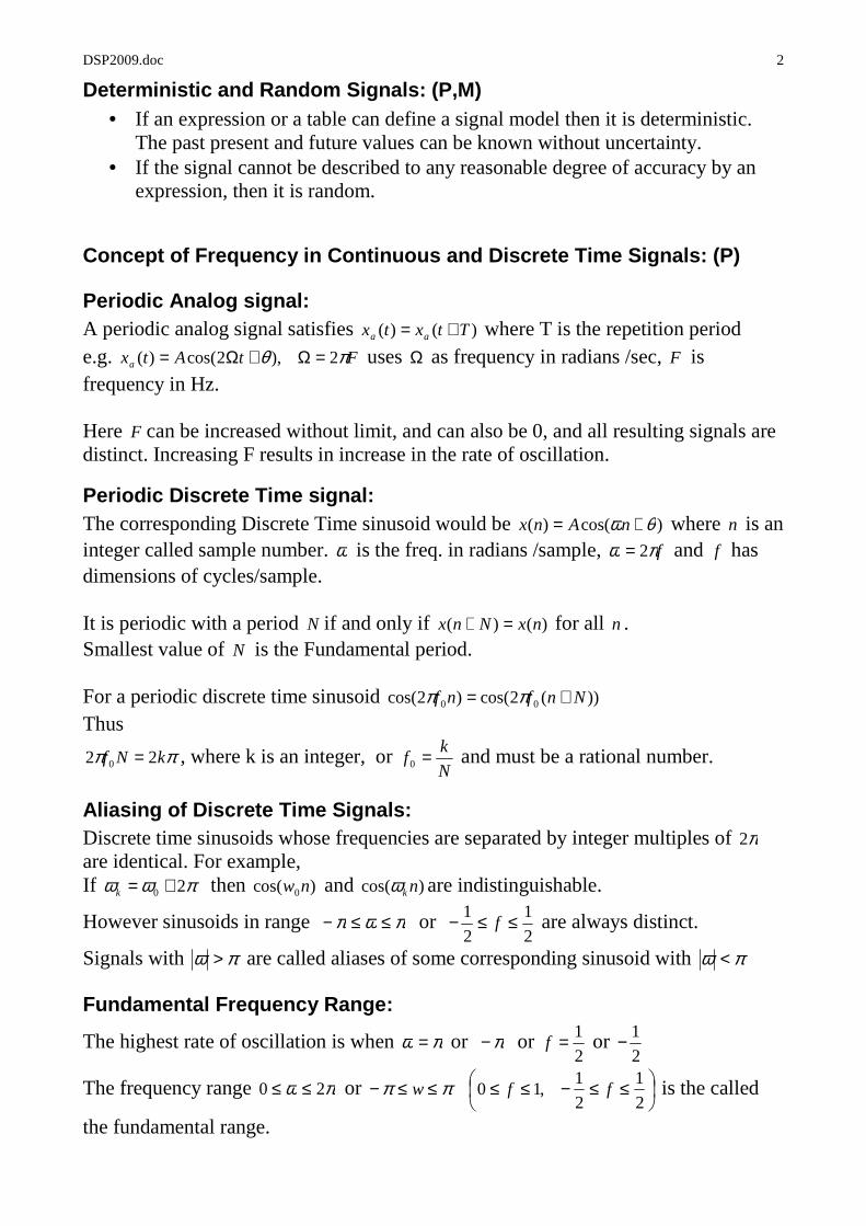
Deterministic and Random Signals: (P,M) • If an expression or a table can define a signal model then it is deterministic.

The past present and future values can be known without uncertainty. • If the signal cannot be described to any reasonable degree of accuracy by an

expression, then it is random.

Concept of Frequency in Continuous and Discrete Tim e Signals: (P)

Periodic Analog signal: A periodic analog signal satisfies )()( Ttxtx aa += where T is the repetition period e.g. FtAtxa πθ 2),2cos()( =Ω+Ω= uses Ω as frequency in radians /sec, F is frequency in Hz. Here F can be increased without limit, and can also be 0, and all resulting signals are distinct. Increasing F results in increase in the rate of oscillation.

Periodic Discrete Time signal: The corresponding Discrete Time sinusoid would be )cos()( θω += nAnx where n is an integer called sample number. ω is the freq. in radians /sample, fπω 2= and f has dimensions of cycles/sample. It is periodic with a period N if and only if )()( nxNnx =+ for all n . Smallest value of N is the Fundamental period. For a periodic discrete time sinusoid ))(2cos()2cos( 00 Nnfnf += ππ Thus

ππ kNf 22 0 = , where k is an integer, or N

kf =0 and must be a rational number.

Aliasing of Discrete Time Signals: Discrete time sinusoids whose frequencies are separated by integer multiples of π2 are identical. For example, If πωω 20 +=k then )cos( 0nw and )cos( nkω are indistinguishable.

However sinusoids in range πωπ ≤≤− or 2

1

2

1 ≤≤− f are always distinct.

Signals with πω > are called aliases of some corresponding sinusoid with πω <

Fundamental Frequency Range:

The highest rate of oscillation is when πω = or π− or 2

1=f or 2

1−

The frequency range πω 20 ≤≤ or

≤≤−≤≤≤≤−2

1

2

1,10 ffw ππ is the called

the fundamental range.

DSP2009.doc 3

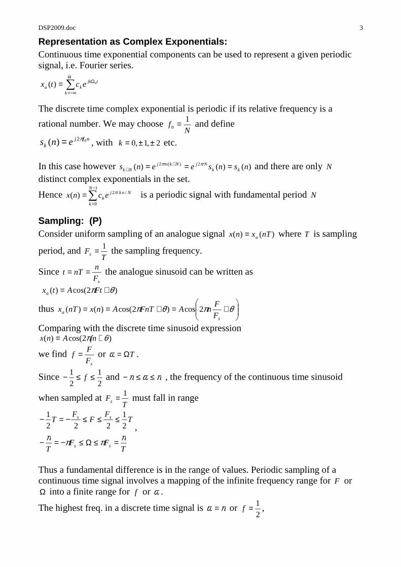
Representation as Complex Exponentials: Continuous time exponential components can be used to represent a given periodic signal, i.e. Fourier series.

The discrete time complex exponential is periodic if its relative frequency is a

rational number. We may choose N

f1

0 = and define

nfjk ens 02)( π= , with 2,1,0 ±±=k etc.

In this case however )()()( 2)(2 nsnseens kk

NjNknjNk === +

+ππ and there are only N

distinct complex exponentials in the set.

Hence ∑−

=

=1

0

/2)(N

k

Nnkjk ecnx π is a periodic signal with fundamental period N

Sampling: (P) Consider uniform sampling of an analogue signal )()( nTxnx a= where T is sampling

period, and T

Fs

1= the sampling frequency.

Since sF

nnTt == the analogue sinusoid can be written as

)2cos()( θπ += FtAtxa

thus

+=+== θπθπ

sa F

FnAFnTAnxnTx 2cos)2cos()()(

Comparing with the discrete time sinusoid expression )2cos()( θπ += fnAnx

we find sF

Ff = or TΩ=ω .

Since 2

1

2

1 ≤≤− f and πωπ ≤≤− , the frequency of the continuous time sinusoid

when sampled at T

Fs

1= must fall in range

TF

FF

T ss

2

1

222

1 ≤≤≤−=−,

TFF

T ss

ππππ =≤Ω≤−=−

Thus a fundamental difference is in the range of values. Periodic sampling of a continuous time signal involves a mapping of the infinite frequency range for F or Ω into a finite range for f or ω .

The highest freq. in a discrete time signal is πω = or 2

1=f ,

∑+∞

−∞=

Ω=k

tjkka ectx 0)(

DSP2009.doc 4

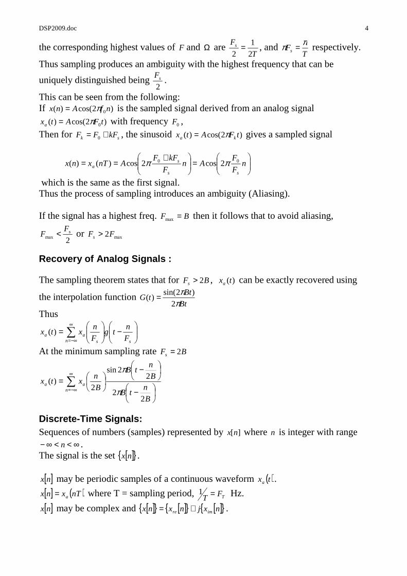
the corresponding highest values of F and Ω are T

Fs

2

1

2= , and

TFs

ππ = respectively.

Thus sampling produces an ambiguity with the highest frequency that can be

uniquely distinguished being 2

sF .

This can be seen from the following: If )2cos()( 0nfAnx π= is the sampled signal derived from an analog signal

)2cos()( 0tFAtxa π= with frequency 0F , Then for sk kFFF += 0 , the sinusoid )2cos()( tFAtx ka π= gives a sampled signal

which is the same as the first signal. Thus the process of sampling introduces an ambiguity (Aliasing). If the signal has a highest freq. BF =max then it follows that to avoid aliasing,

2maxsF

F < or max2FFs >

Recovery of Analog Signals :

The sampling theorem states that for BFs 2> , )(txa can be exactly recovered using

the interpolation function Bt

BttG

ππ

2

)2sin()( =

Thus

∑∞

−∞=

−

=

n ssaa F

ntg

F

nxtx )(

At the minimum sampling rate BFs 2=

∑∞

−∞=

−

−

=n

aa

B

ntB

B

ntB

B

nxtx

22

22sin

2)(

π

π

Discrete-Time Signals: Sequences of numbers (samples) represented by ][nx where n is integer with range

∞<<∞− n . The signal is the set [ ] nx .

[ ]nx may be periodic samples of a continuous waveform ( )txa .

[ ] ( )nTxnx a= where T = sampling period, TFT =1 Hz.

[ ]nx may be complex and [ ] [ ] [ ] nxjnxnx imre += .

=

+== n

F

FAn

F

kFFAnTxnx

ss

sa

00 2cos2cos)()( ππ

DSP2009.doc 5

Types of Sequences: (M) Finite: A sequence is finite if ∞<<∞−>≤≤ 211221 ,,, NNNNNnN Length is defined as 121 −+= NNN (N point sequence) Such a sequence can be made infinite by assigning zero values outside defined range.

[ ]418.02050.6705.04.95.3][ −=nh Above sequence is defined from 32 ≤≤− n . It can be made infinite by defining 0][ =nh for 3,2 >−< nn . Infinite: Right Sided. Zero values for 11, NNn < negative or positive.

20][ −<= nnx , and 2][ −≥= nnnx

If 01 ≥N then CAUSAL.

Left Sided: zero for 2Nn > . If 02 ≤N then ANTI CAUSAL.

( ) 51][ −≤−= nnnx 5 0][ −>= nnx

Two Sided: Has ∞≤≤∞− n .

21][ nnx =

Even / Odd: Conjugate symmetric ][][ nxnx −= ∗ If all ][nx real then EVEN Conjugate asymmetric ][][ nxnx −−= ∗ , If all ][nx real then ODD

Periodic: ][][ kNnxnx += for all n , N is a positive integer, and is the PERIOD of sequence

fN = fundamental period is the period with smallest N

Bounded:

[ ] ∞<≤ xBnx 00][ ≤= nnx

01][ >= nnnx Absolutely Summable:

[ ] ∞<∑ nx

DSP2009.doc 6

Square Summable:

[ ] ∞<=∑2

nxE , E is the energy

Basic Sequences: (M) Unit Sample:

00][

01][

≠===

nn

nn

δδ

Unit Step:

00][

01][

<=≥=

nn

nn

µµ

∑= ][][ kn δµ ]1[][][ −−= nnn µµδ

Exponential:

[ ] nAnx α= , where A , α are complex in general and 00 ωσα je += , Φ= jeAA .

[ ] ( )Φ+= neAnx nre 0cos0 ωσ

[ ] ( )Φ+= neAnx nim 0sin0 ωσ

For a real sinusoid ( )Φ+= nAnx 0cos][ ω , 0ω is angular frequency. In Phase Sequence: For a real sinusoid sequence ][][][ nxnxnx qi += ,

)cos(cos][ 0nAnxi ωφ= is the in-phase sequence Quadrature Sequence:

)sin(sin][ 0nAnxq ωφ−= is the quadrature sequence. Complex exponential sequence with 00 =σ and real sinusoidal sequence are periodic with period N as long as rn πω 20 = where r is an integer.

Or rN=

0

2ω

π .

Thus Periodic only if 0

2ω

π is rational.

Operations on Sequences: (M) Product:

][][][ nynxnw •= i.e. in modulation, windowing Addition:

][][][ nynxnw +=

Scalar multiplication:

][][ nAxnw =

DSP2009.doc 7

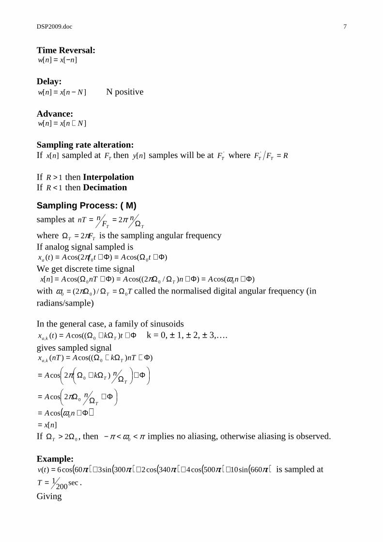
Time Reversal:

][][ nxnw −= Delay:

][][ Nnxnw −= N positive Advance:

][][ Nnxnw +=

Sampling rate alteration: If ][nx sampled at TF then ][ny samples will be at '

TF where RFF TT =' If 1>R then Interpolation If 1<R then Decimation

Sampling Process: ( M)

samples at TT

nF

nnT Ω== π2

where TT Fπ2=Ω is the sampling angular frequency If analog signal sampled is

)cos()2cos()( 00 Φ+Ω=Φ+= tAtfAtxa π We get discrete time signal )cos())/2cos(()cos(][ 000 Φ+=Φ+ΩΩ=Φ+Ω= nAnAnTAnx T ωπ with TT 000 /)2( Ω=ΩΩ= πω called the normalised digital angular frequency (in radians/sample) In the general case, a family of sinusoids

Φ+Ω+Ω= tkAtx Tka )cos(()( 0, k = 0, ± 1, ± 2, ± 3,….

gives sampled signal

( )][

cos

2cos

)2cos

))cos(()(

0

0

0

0,

nx

nA

nA

nkA

nTkAnTx

T

TT

Tka

=Φ+=

Φ+ΩΩ=

Φ+

ΩΩ+Ω=

Φ+Ω+Ω=

ω

π

π

If 02Ω>ΩT , then πωπ <<− 0 implies no aliasing, otherwise aliasing is observed. Example:

( ) ( ) ( ) ( ) ( )ttttttv πππππ 660sin10500cos4340cos2300sin360cos6)( ++++= is sampled at

sec2001=T .

Giving

DSP2009.doc 8

( ) ( ) ( ) ( ) ( )nnnnnnv πππππ 3.3sin105.2cos47.1cos25.1sin33.0cos6)( ++++= ( ) ( )( ) ( )( ) ( )( ) ( )( )nnnnnnv πππππππππ 7.04sin105.02cos43.02cos25.02sin33.0cos6)( −+++−+−+=( ) ( )nnnnv πππ 7.0sin106435.05.0cos(53.0cos8)( +++=

Same results are obtained if w(t) = 8 cos (60πt) + 5 cos (100πt + 0.6435) -10 sin (140πt) are sampled at the same rate.

Linear Systems: (M, P) Input x[n] = α x1[n] + β x2[n] gives an output y[n] = α y1[n] + β y2[n] for all α, β, x1, and x2

example: y[n] = nx[n] is linear y1[n[ = nx1[n], y2[n] = nx2[n] thus y3[n] = n([a1x1[n] + a2x2[n]) also a1y1[n] +a2y2[n] = a1nx1[n] + a2nx2[n] . y[n] = x[n2] is linear y1[n] = x1[n

2] and y2[n] = x2[n2] hence y3[n] = a1 x1[n

2] + a2 x2[n2]

linear combination of outputs is a1y1[n] +a2y2[n] = a1 x1[n2] + a2 x2[n

2] y[n] = x2[n] is non-linear y1[n] = x1

2[n] and y2[n] = x22[n] hence y3[n] = (a1 x1[n] + a2 x2[n])2

linear combination of outputs is a1y1[n] +a2y2[n] = a1 x12[n] + a2 x2

2[n] y[n] = Ax[n] + B is linear only if B = 0 y1[n] = Ax1[n] + B and y2[n] = Ax2[n] + B hence y3[n] = A(a1 x1[n] + a2 x2[n]) + B linear combination of outputs is a1y1[n] +a2y2[n] = Aa1x1[n] + a1B + Aa2x2[n] + a2B Accumulator [ ] [ ]∑= nxny

y[n] = ∑ (α x1[k] + β x2[k]) = α ∑ x1[k] + β ∑ x2[k] = α y1[n] + β y2[n] is linear Accumulator with an initial condition (Causal accumulator) has

∑=

+−=n

k

kxyny0

111 ][]1[][ and ∑=

+−=n

k

kxyny0

222 ][]1[][

Hence for input α x1[n] + β x2[n]

∑=

++−=n

l

kxkxyny0

2111 ][][]1[][ βα = ∑∑==

++−n

k

n

k

kxkxy0

20

1 ][][]1[ βα

but

∑∑==

+−++−=+n

k

n

k

kxykxynyny0

220

1121 ][]1[][]1[][][ ββααβα

DSP2009.doc 9

which can equal y[n] only if y[-1] = α y1[-1] + β y2[-1] for all α, β, y[-1], y1[-1] and y2[-1]. This is possible if and only if system starts from rest with initial condition zero. Otherwise it is Nonlinear

Shift Invariance: (Time Invariance) (M,P) If x[n] → y[n] then x[n-n0] → y[n-n0] Y[n] = x[n] – x[n-1] is time invariant If input is delayed and applied y(n,k) = x(n-k) – x(n-k-1) If output is delayed y(n-k) = x(n-k) – x(n-k-1) Y[n] = nx[n] is time variant Response to x(n-k) is y(n,k) = nx(n-k) However if output is delayed, y(n-k) = (n-k)x(n-k) Y[n] = x[-n] is time variant Response to x(n-k) is y(n,k) = x(-n-k) However if output is delayed, y(n-k) = (-n+k) Y[n] = x[n]cos(wn) is time variant

Linear Time Invariant (LTI): A system having both Linear and Time-invariance properties.

Causality: y[n0] depends only on x[n] where n ≤ n0

Stability: Bounded input gives bounded output (BIBO Stability) if |x[n]| < Bx then |y[n]| < By

Impulse Response And Step Response:

Impulse Response: denoted by h[n] is the response to a unit sample sequence δ[n]

Step Response: S[n] → response to µ [n]

Response To Signal x[n]: (M,P)

Expressing [ ]nx sequence as ∑+∞=

−∞=

−=k

k

knkxnx )(][][ δ the response of LTI system to

)(][ knkx −δ will be [ ] [ ]knhkx −

DSP2009.doc 10

Thus [ ] [ ] [ ]∑ −= knhkxny or by a change of variables

[ ] [ ] [ ]∑ −= khknxny

which is a convolution [ ] [ ]nhnx ∗ example:

[ ]31102 −−=a , [ ]1021 −=b [ ]31513142 −−−=∗ ba

Because of the summation both [ ]nx and [ ]ny cannot be infinite. Convolution of sequence of lengths M and N gives a sequence of length M+N-1 Convolution is commutative, associative and distributive.

Stability Condition For LTI System: (P) ∞<=∑ ][nhS

Causality Condition: (P) 0][ =nh for 0<n

For a Causal sequence input into a causal LTI system

i.e. 0][ =ny for 0<n and is thus also causal

Classes of LTI Systems: (P)

FIR: Finite Impulse Response

if h[n] is of finite length 0][ =nh for 1Nn < and 2Nn > with 21 NN < .

Impulse response is zero outside a finite time interval. Causal FIR system has 0][ =nh for 0<n and Mn ≥

The convolution equation for causal FIR is Output is the weighted linear combination of the past M input samples. Has a memory of M samples. It can be realised by adders, multipliers and finite memory.

IIR: infinite impulse response

IIR if h[n] is of infinite length. In a causal IIR summation in the convolution is from k = 0 to ∞ It involves all the past input samples, and requires infinite memory. So realisation by convolution ∑ form is impractical. A more practical way is by the difference equation form.

∑∑==

−=−=n

k

n

k

knhkxknxkhny00

][][][][][

∑−

=

−=1

0

][][][M

k

knxkhny

DSP2009.doc 11

Example: cumulative average of x[n] in 0 ≤ k ≤ n Knowledge of all input samples required, and therefore an increasing memory requirement with time. However rewriting the above expression as:

The expression is recursive, and calculation requires 2 multiplication, 1 addition and 1 memory location ]1[ −ny Recursive System: Systems whose output depends on past output values. In the previous example

][1

1]1[

1][ 0

00

0

00 nx

nny

n

nny

++−

+=

]1[ 0 −ny is the initial condition at 0nn = . Computation of the output of a recursive system at a time say 0n requires computation of the previous values of ][ky in correct order. Non-Recursive System: Such systems depend only on the present and past inputs. Causal FIR systems are non-recursive. Their computation can be in any order Simple Recursive System: Let ][]1[][ nxnayny +−= & let initial condition be ]1[−y

]0[]1[]0[ xayy +−= ]1[]0[]1[]1[]0[]1[ 2 xaxyaxayy ++−=+=

]2[]1[]0[]1[]2[]1[]2[ 23 xaxxayaxayy +++−=+= or

For an initially relaxed system 0]1[ =−y , and the output is the zero-state response or the Forced response. For a non-relaxed system, with 0][ =nx for all n , output is called zero input response or Natural or Free response.

Finite Dimensional LTI System: (M)

KK 1,0][1

1][

0

=+

= ∑=

nkxn

nyn

k

0][]1[][0

1 ≥−+−= ∑=

+ nknxayanyn

k

knLL

][1

1]1[

1][

][]1[][][][)1(1

0

nxn

nyn

nny

nxnnynxkxnynn

++−

+=

∴

+−=+=+ ∑−

DSP2009.doc 12

A sub-class of LTI system characterised by a linear constant coefficient difference equation:

][][00

knxpknydM

kk

N

kk −=− ∑∑

==

where

kd and kp are constants, MN ≥ and N is the order of the equation.

Linearity, Time Invariance and Stability: (P)

Constant coefficient linear difference equation implies a time invariant system.

BIBO:

Bounded Input Bounded Output Stable if and only if for every bounded input and every bounded initial condition the total system response is bounded. Example:

][]1[][ nxnayny +−= Assume ][nx is bounded i.e. ∞≤≤ xMnx ][ for all 0≥n . Then

∑=

+ −+−≤n

k

kn knxayany0

1 ][]1[][

∑=

+ +−≤n

k

k

xn aMyany

0

1 ]1[][

y

n

x

nM

a

aMyany =

−−

+−≤+

+

1

1]1[][

11

If n is finite yM is finite irrespective of a , but as ∞→n , yM is finite only if 1<a .

Thus system is stable only if 1<a .

Z-Transform and Transfer Functions:

Direct z-transform: (P)

x[n] has a z-transform X(z) given by

where z is complex. The infinite series converges for a set of values of z (Region of Convergence – ROC) examples:

∑∞

−∞=

−=n

nznxzX ][)(

DSP2009.doc 13

1. [ ]107521][ =nx 5321 7521)( −−−− ++++= zzzzzX ; ROC entire z-plane except z = 0

2. [ ]107521][ =nx 312 7521)( −− ++++= zzzzzX ; ROC entire z-plane except z = 0, ∞

3. [ ]10752100][ =nx 75432 752)( −−−−− ++++= zzzzzzX ; ROC entire z-plane except z = 0

4. ][][ nnx δ= 1)( =zX ; ROC entire z-plane

5. 0],[][ >−= kknnx δ , kzzX −=)( ; ROC entire z-plane except z = 0

6. 0],[][ >+= kknnx δ kzzX =)( ; ROC entire z-plane except z = ∞

x[n] having infinite duration can be described by a closed form expression in z (infinite geometric series) example:

][][ nunx nα= i.e. nα when 0≥n and 0 when 0<n has

in closed form this is expressed as 11

1−− zα

, ROC α>z

however if ]1[][ −−−= nunx nα i.e. 0 when 0≥n and nα− when 1−≤n ,

in closed form this is expressed as 11

1−− zα

, ROC α<z

Thus the z-transform is the same for both series, only the region of convergence differs. Therefore it needs to be stated to uniquely identify the sequence.

]1[][][ −−+= nubnunx nnα

has The first converges for α>z , the second for bz <

If | b |<| α | ROCs do not overlap and hence X(z) does not exist If | b | > | α | ROCs do overlap giving a ring in the z-plane where both terms converge. Hence X(z) exists, with ROC |α| < |z| < |b|. This is the general case with two-sided infinite duration signals

∑∑∞

−∞

− ==0

1

0

)()( nnn zzzX αα

∑∑−

∞−

−∞

− +=1

0

)( nnnn zbzzX α

DSP2009.doc 14

POLES and ZEROS of Z-transform: (P)

If X(z) is rational then

Which can be expressed as

where 0

0a

bG = , then there are M finite zeros, N finite poles and N - M zeros

(if N > M) or poles (if N < M) at the origin. Zeros and poles may also exist at ∞ The ROC of the z-transform does not contain poles, and is bounded by them. Effect of Pole position on Impulse Response

Poles inside unit circle give bounded output, faster decay as pole is nearer to origin. poles outside unit circle give unbounded output and hence unstable single pole- if signal is real pole also must be real. –ve pole causes signal to alternate in sign. The signal x(n) = anu(n) has transform X(z) = 1/(1-az-1), zero at 0 pole at a

NN

MM

zazaa

zbzbb

zD

zNzX −−

−−

++++++

==....

....

)(

)()(

110

110

∏

∏

−

−= −

N

k

M

kMN

pz

zzGzzX

1

1

)(

)()(

DSP2009.doc 15

∑∑ == −M

kM

MkM

k zbz

zbzH00

1)(

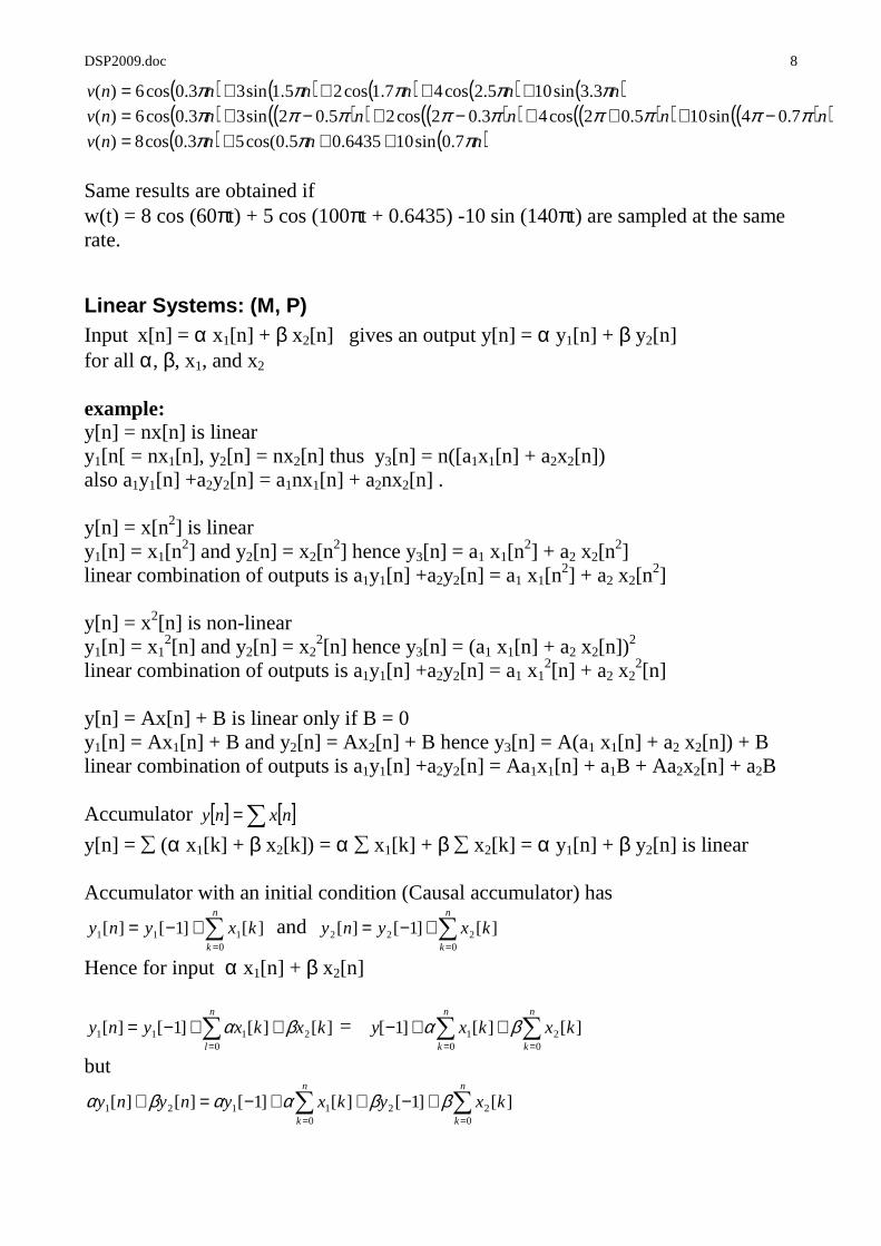
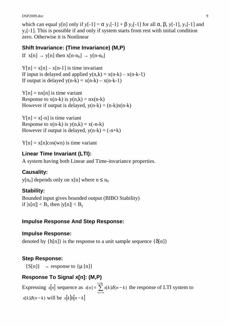
double real poles in expression of type x[n] = nanu[n].even on unit circle unbounded increase. complex conjugates → exponentially weighted sinusoid, envelope varies as rn, frequency on angle.

double complex → even on unit circle increasing envelope Poles inside unit circle give bounded output, faster decay as pole is nearer to origin. poles outside unit circle give unbounded output and hence unstable

Transfer Function:

Let system have a linear coefficient difference equation

taking z- transform with time shifting

hence in above equation if ak=0 then for 1 ≤ k ≤ n

∑∑ −+−−=M

k

N

k knxbknyany01

][][][

∑ ∑ −− +−=N M

kk

kk zzXbzzYazY

1 0

)()()(

DSP2009.doc 16

The multiple M poles at 0 are trivial, and there are M nontrivial zeros. This is an All-Zero system, It has a finite duration Impulse response (FIR). If bk= 0 for 1 ≤ k ≤ n the system is an All-Poles system. Its impulse response is infinite duration (IIR). In the general case both poles and zeros exist. Because of the poles the system will be IIR.

Frequency response: (M)

The frequency response is the complex DTFT of the LTI system.

Its magnitude is the magnitude response and its angle is the phase response. G(w) = 20 log10| H(ejw) | dB is the GAIN function and – G(w) is called Attenuation or LOSS function. For a real impulse response h[n] magnitude response is even and phase response is odd. The negative of derivative of the angle θ(w) w.r.t. w is called the GROUP DELAY. For the LTI system Y(ejw) = H(ejw).X(ejw) If the system is characterised by a constant coefficient difference equation

then

The transfer function is a generalisation of the frequency response. It is the z-transform of h[n], has real coefficients and is a rational polynomial in z-1.

∑ −=2

1

][)(N

N

nznhzH

The frequency response is the transfer function evaluated at z = ejw. For a FIR filter, we have. Then for a causal FIR filter N1= 0 and N2 > 0, all poles are at the origin, and ROC is the entire z-plane except z = 0. For a finite dimensional IIR characterised by a difference equation the transfer function is a rational expression

which can be written as

∑+∞

∞−

−= jwnjw enheH ][)(

∑ ∑= =

−=−N

k

M

kkk knxpknyd

0 0

][][

∑

∑

=

−

=

−

=N

k

jwkk

M

k

jwkk

jw

ed

epeH

0

0)(

NN

MM

zdzdzdd

zpzpzppzH −−−

−−−

++++++++

=L

L

22

110

22

110)(

DSP2009.doc 17

where ξ1, ξ2, are the finite zeros and λ1, λ2 etc are the finite poles. There are additional N-M zeros or poles at origin.

• FIR transfer function is always stable, For IIR all poles must be within the unit circle for stability.

• Poles and zeros determine the filter behaviour, and may be placed to obtain a particular frequency response.

• Poles near the points (but inside unit circle) emphasise the frequency corresponding to the point on the circle.

• Zeros may be placed near frequency to be de-emphasised, and need not be within the unit circle.

• Complex zeros and poles must occur in conjugate pairs to make filter coefficients real

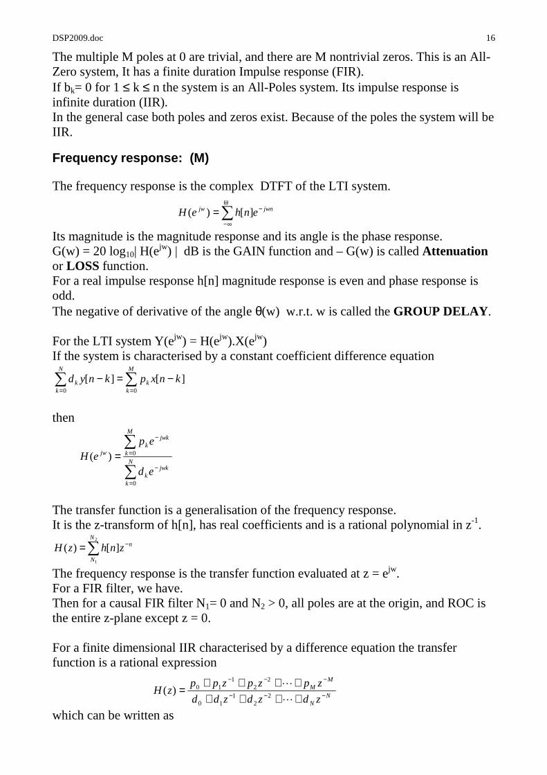
Geometric evaluation of the Frequency Response: (P)

The z-transform of the LTI system may be expressed in terms of its poles and zeros

for N = M for simplicity

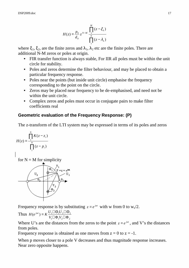
Frequency response is by substituting jwtez = with w from 0 to ws/2.

Thus 2211

2211)(Φ∠Φ∠Θ∠Θ∠

=VV

UUKeH jwt

Where U’s are the distances from the zeros to the point jwtez = , and V’s the distances from poles. Frequency response is obtained as one moves from z = 0 to z = -1.

When p moves closer to a pole V decreases and thus magnitude response increases. Near zero opposite happens.

∏

∏

−

−= −

N

k

M

kMN

z

zz

d

pzH

1

1

0

0

)(

)()(

λ

ξ

∏

∏

−

−=

N

i

N

i

pz

zzKzH

1

1

)(

)()(

DSP2009.doc 18

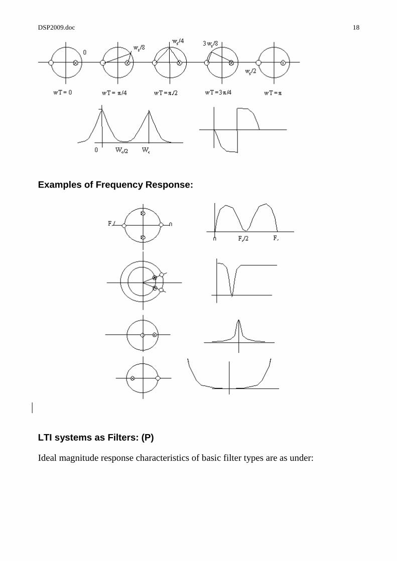
Examples of Frequency Response:

LTI systems as Filters: (P)

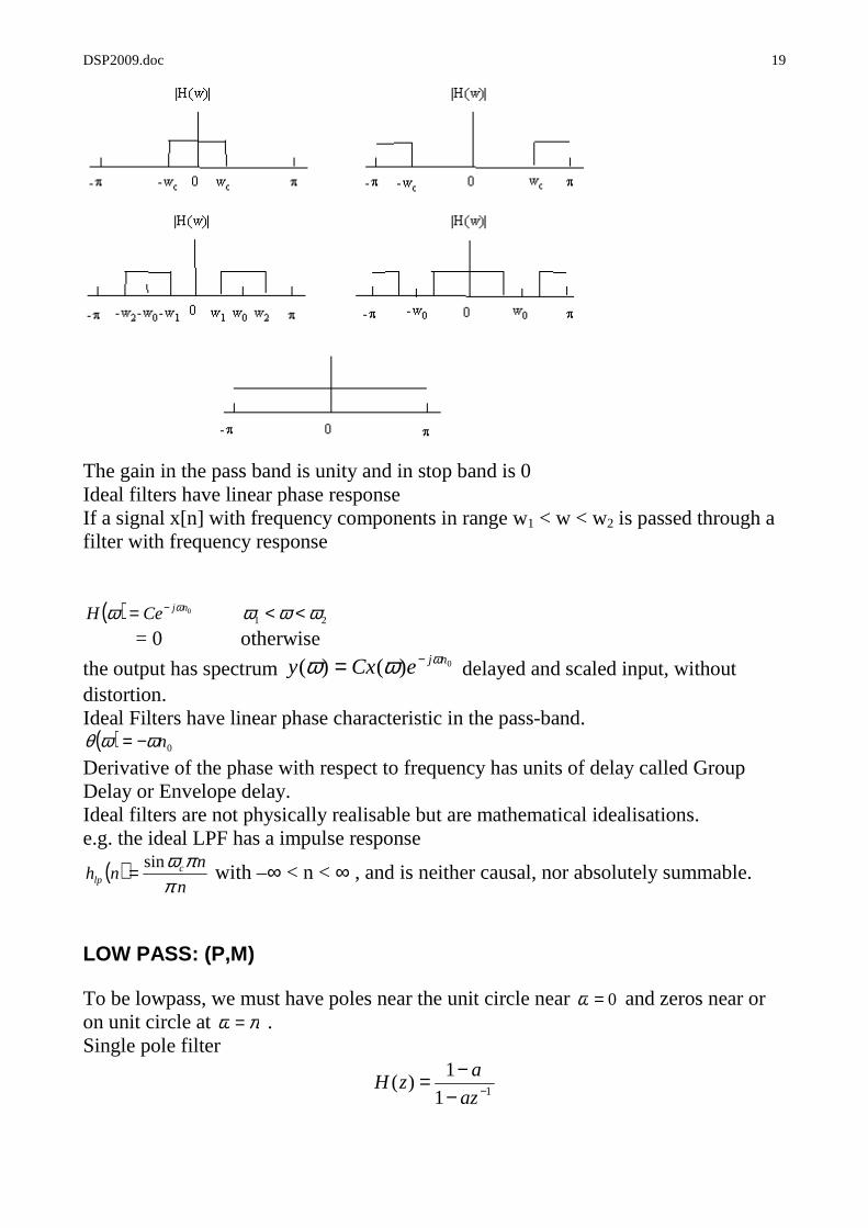
Ideal magnitude response characteristics of basic filter types are as under:

DSP2009.doc 19

The gain in the pass band is unity and in stop band is 0 Ideal filters have linear phase response If a signal x[n] with frequency components in range w1 < w < w2 is passed through a filter with frequency response

( ) 0njCeH ωω −= 21 ωωω << = 0 otherwise

the output has spectrum 0)()( njeCxy ωωω −= delayed and scaled input, without distortion. Ideal Filters have linear phase characteristic in the pass-band.

( ) 0nωωθ −=

Derivative of the phase with respect to frequency has units of delay called Group Delay or Envelope delay. Ideal filters are not physically realisable but are mathematical idealisations. e.g. the ideal LPF has a impulse response

( )n

nnh c

lp ππωsin

= with –∞ < n < ∞ , and is neither causal, nor absolutely summable.

LOW PASS: (P,M)

To be lowpass, we must have poles near the unit circle near 0=ω and zeros near or on unit circle at πω = . Single pole filter

11

1)( −−

−=az

azH

DSP2009.doc 20

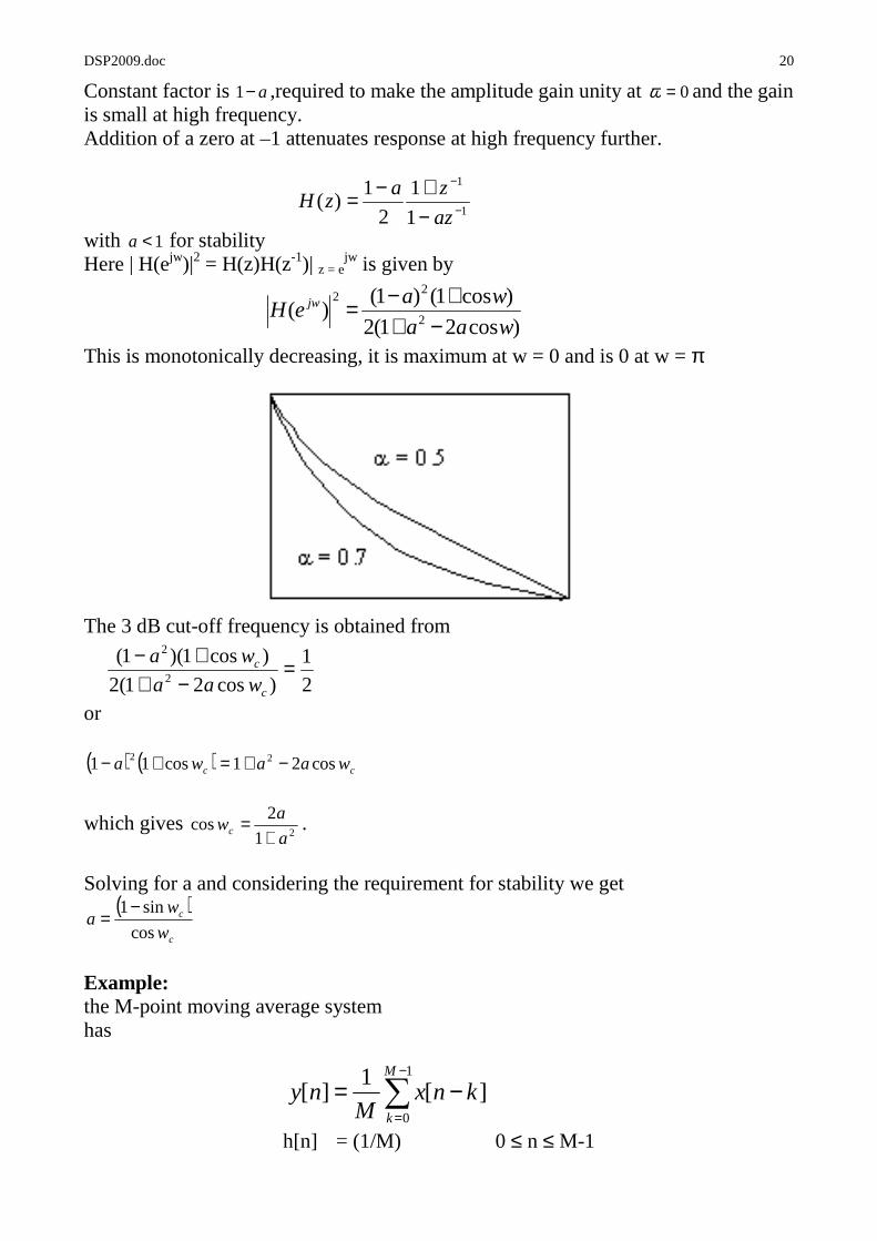
Constant factor is a−1 ,required to make the amplitude gain unity at 0=ω and the gain is small at high frequency. Addition of a zero at –1 attenuates response at high frequency further.

with 1<a for stability Here | H(ejw)|2 = H(z)H(z-1)| z = e

jw is given by

This is monotonically decreasing, it is maximum at w = 0 and is 0 at w = π

The 3 dB cut-off frequency is obtained from

or ( ) ( ) cc waawa cos21cos11 22 −+=+−

which gives 21

2cos

a

awc +

= .

Solving for a and considering the requirement for stability we get

( )c

c

w

wa

cos

sin1−=

Example: the M-point moving average system has

h[n] = (1/M) 0 ≤ n ≤ M-1

)cos21(2

)cos1()1()(

2

22

waa

waeH jw

−++−=

2

1

)cos21(2

)cos1)(1(2

2

=−+

+−

c

c

waa

wa

1

1

1

1

2

1)( −

−

−+−=

az

zazH

][1

][1

0

knxM

nyM

k

−= ∑−

=

DSP2009.doc 21

= 0 otherwise with M = 2 the transfer function is

H(z) = ½(1 + z-1) Its frequency response is

H(jw) = e-jw/2 cos(w/2) Thus magnitude response | H(ejw) | = cos(w/2) is monotonically decreasing from w = 0 to w = π and the –3 dB frequency is at cos2(wc/2) = ½ i.e. at π/2 a cascade of M such sections has wc = 2cos-1(2-1/2M) for M =3 wc = 0.3 π and thus higher order has a sharper cut-off. A higher order moving average filter will be an even better approximation to ideal LP filter. Example: A two pole LP filter is H(z) = b0/(1−pz-1)2

Determine b0 and p such that H(0) = 1 and |H(π/4)|2 = ½ Here when w = 0 H(ej0) = b0/(1-p)2 = 1 at w = 0 so b0 = (1-p)2 At w = π / 4 H(ejπ/4)= (1-p)2 / (1-pe-j π /4)2 = (1-p)2 / (1-p Cos(π /4) + j p sin(π /4))2

= (1-p)2 / (1-p/√2 + jp/√2)2

Then (1-p)4 / [(1-p/√2)2 + p2/2] 2 = ½ Or √2(1-p)2 = 1 + p2 – √(2p) Solution is p = 0.32 giving H(z) = 0.46 / (1- 0.32z-1)2

High Pass: (P,M)

Translating Hlp (w) by π radians (i.e. replacing w by w - π) converts it into a HP filter. i.e. Hhp(w) = Hlp(w - π) The frequency translation of π is equivalent to multiplication of impulse reponse hlp by e jπn

Thus hhp(n) = (e jπ)n hlp(n) = (−1)n hlp(n) This means changing signs of the odd samples in hlp(n) Conversely, hlp(n) = (−1)n hhp(n) Proof: Let the LPF be described by the difference equation

∑∑==

−+−−=M

kk

N

kk knxbknyany

01

)()()(

DSP2009.doc 22

1

1

1

1

2

1)( −

−

+−−=

az

zazH

Its frequency response is

replacing w by w- π gives

corresponding to the difference equation

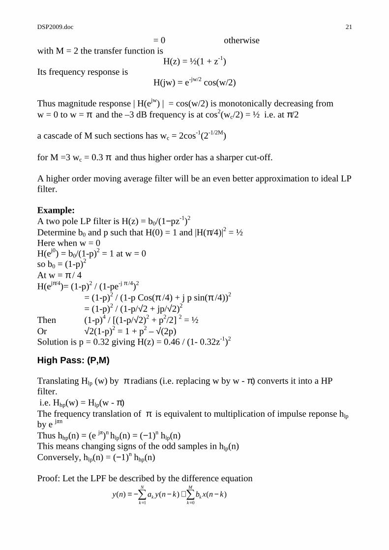
Example: The LPF y(n) = 0.9y(n-1) + 0.1x(n) give HPF y(n) = -0.9y(n-1) + 0.1x(n) with frequency response as Hhp(w) = 0.1/(1+0.9e –jw) Thus high pass single pole amplifier

has the response

To get a HP FIR filter replace z in the moving average filter with –z to get H(z) = ½ (1-z-1). For M = 2, This has H(ejw) = e-jw/2 sin(w/2) a higher order filter of the form

yields a sharper HP response.

Band- Pass Filter and Band- Stop Filter: (M,P)

A Band pass filter should contain one or more pairs of complex conjugate poles near the unit circle, near the frequency band that is the pass-band.

∑−

=

−−=1

0

)1(1

)(M

n

nn zM

zH

∑∑==

−−+−−−=M

kk

kN

kk

k knxbknyany01

)()1()()1()(

∑

∑

=

−

=

−

−+

−= N

k

jwkk

k

M

k

jwkk

k

hp

ea

ebwH

1

0

)1(1

)1()(

∑

∑

=

−

=

−

+= N

k

jwkk

M

k

jwkk

lp

ea

ebwH

0

0

1)(

21

2

)1(1

1

2

1)( −−

−

++−−−=

azza

zazH

β

DSP2009.doc 23

Has centre frequency w0 = cos-1(β) and 3-dB bandwidth = cos-1 (2a/(1+a2)) A band stop filter has zero on the unit circle at the frequency w0, and has a transfer function of the form

Its notch frequency is w0 = cos-1(β) and 3-dB bandwidth is cos-1 (2a/(1+a2)) like in the BPF. Example: Design a two pole BPF with pass-band centred at w = π/2 zeros at w = 0 and π and magnitude response is 1/√2 at w = 4 π / 9 Let the poles be p1,2 = re± j π /2 and zeros be at –1 and 1 Then

The frequency response at π/2 is

( ) 11

2

2 2=

−=

rGH

π

or G = (1-r2)/2 Evaluating |H(4 π/9)|2 at w = 4 π/9

which gives 1.94(1-r2)2 = 1 − 1.88 r2 + r4 which is having solution r2 = 0.7, so the system function is H(z) = (0.15)(1−z -2)/(1+ 0.7z−2)

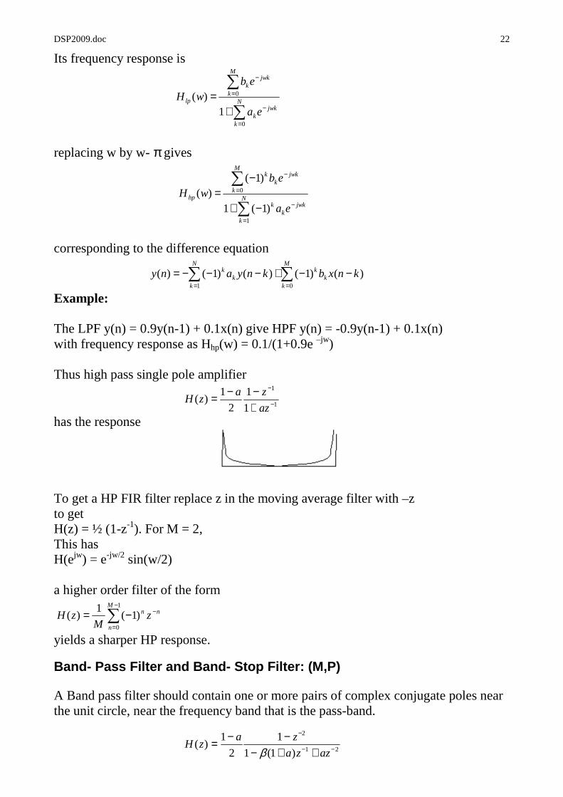
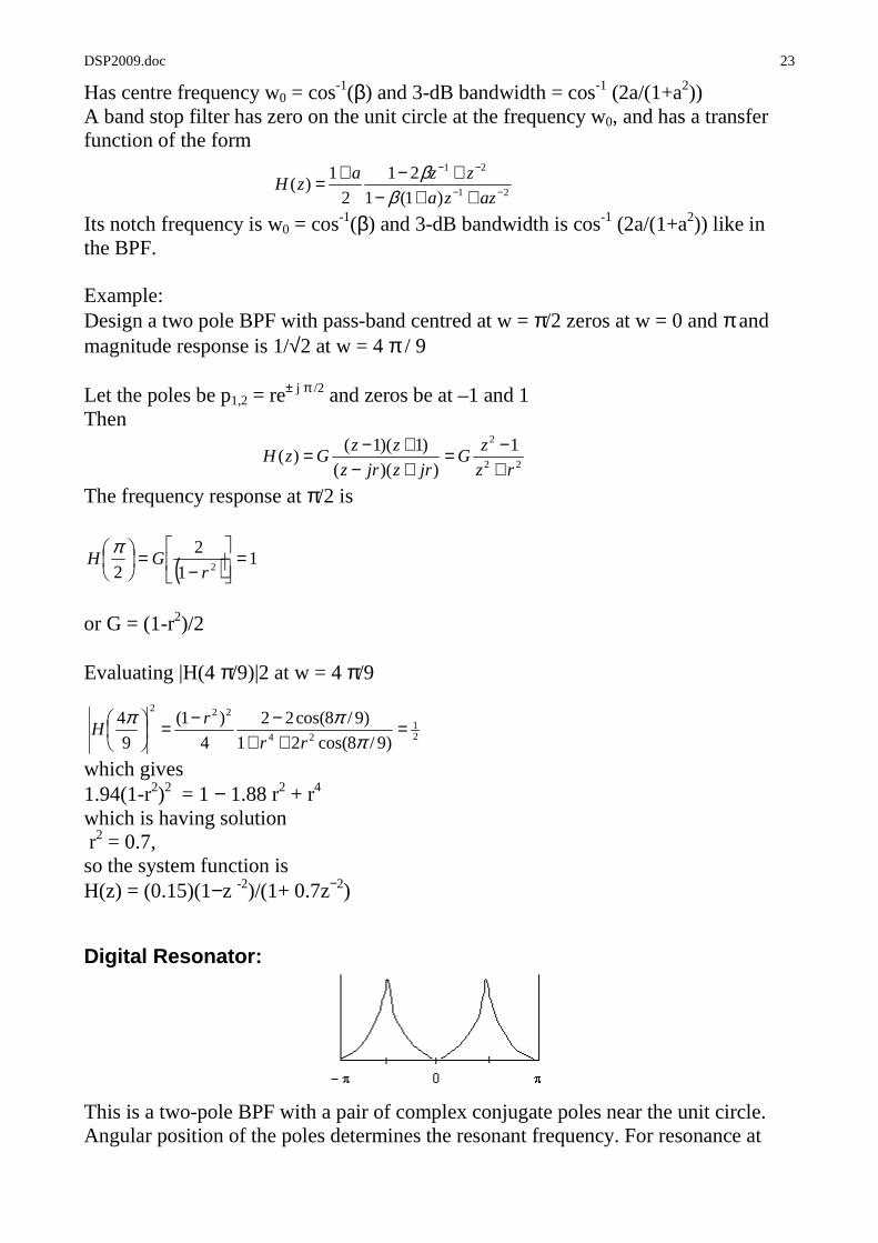
Digital Resonator:

This is a two-pole BPF with a pair of complex conjugate poles near the unit circle. Angular position of the poles determines the resonant frequency. For resonance at

22

2 1

))((

)1)(1()(

rz

zG

jrzjrz

zzGzH

+−=

+−+−=

21

24

222

)9/8cos(21

)9/8cos(22

4

)1(

9

4 =++

−−=

πππ

rr

rH

21

21

)1(1

21

2

1)( −−

−−

++−+−+=

azza

zzazH

ββ

DSP2009.doc 24

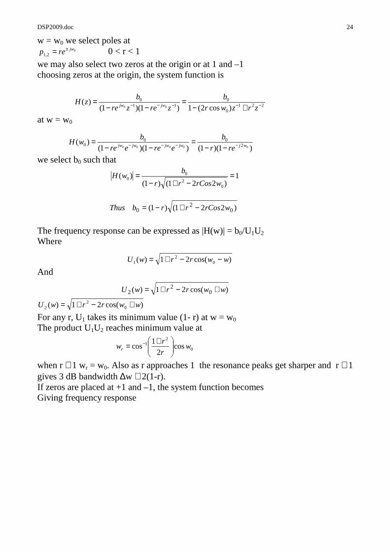
)cos(21)( 02

2 wwrrwU +−+=

w = w0 we select poles at 0

2,1jwrep ±= 0 < r < 1

we may also select two zeros at the origin or at 1 and –1 choosing zeros at the origin, the system function is

at w = w0

we select b0 such that

The frequency response can be expressed as |H(w)| = b0/U1U2 Where

And

)cos(21)( 02

2 wwrrwU +−+=

For any r, U1 takes its minimum value (1- r) at w = w0 The product U1U2 reaches minimum value at

when r ≅ 1 wr = w0. Also as r approaches 1 the resonance peaks get sharper and r ≅ 1 gives 3 dB bandwidth ∆w ≅ 2(1-r). If zeros are placed at +1 and –1, the system function becomes Giving frequency response

2210

011

0

)cos2(1)1)(1()(

00 −−−−− +−=

−−=

zrzwr

b

zrezre

bzH jwjw

)1)(1()1)(1()(

00000 200

0 wjjwjwjwjw rer

b

ereere

bwH −−−− −−

=−−

=

)221()1( 02

0 wrCosrrbThus −+−=

1)221()1(

)(0

2

00 =

−+−=

wrCosrr

bwH

)cos(21)( 02

1 wwrrwU −−+=

0

21 cos

2

1cos w

r

rwr

+= −

DSP2009.doc 25

The amplitude response is |H(w)| = b0N(w)/U1(w)U2(w) where N(w) is defined as above. Thus the resonant frequency and bandwidth are altered by the added zeros.

Digital Oscillator: (P)

A two pole resonator for which the poles lie on the circle.

has complex conjugate poles at 0ωjre± and unit sample response h[n] = [bor

n/(sin wo)]×sin(n+1)wou(n) If r = 1, bo = A sinwo then h[n] =A sin(n+1)wou(n) giving sinusoidal oscillations.

Notch filters: (P)

Used to eliminate specific frequencies. E.g. power line frequency and its harmonics. To create a notch at w0 introduce a pair of conjugate complex zeros at angle w0 on the unit circle.

02,1

ωjez ±=

Thus system function for a FIR notch filter would be )cos21()1)(1()( 21

011

000 −−−−− +−=−−= zzzezebzH jj ωωω

The notch will have a large bandwidth. This can be reduced by adding a pair of complex poles at 0

2,1ωjrep ±=

The poles introduce resonance and reduce bandwidth. The system transfer function is then:

2210

2

11

11

)cos2(1

1

)1)(1(

)1)(1()(

00 −−−−−

−−

+−−=

−−+−=

zrzwr

zG

zrezre

zzGzH

jwjw

[ ][ ])()(

2

0 00 11

1)( wwjwwj

wj

rere

ebwH +−

−

−−−=

wwN 2cos1(2)( −=

2210

0

)cos2(1)( −− +−

=zrzwr

bzH

z z2rcosw-1

z z2cosw-1)(

2-21-0

-2-10

0 rbzH

++=

DSP2009.doc 26

Introduction of a pole near the zero may result in a ripple in the pass-band, which may be removed by adding more poles and zeros.

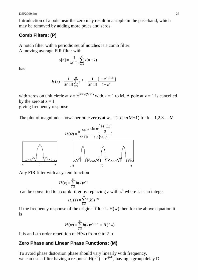
Comb Filters: (P)

A notch filter with a periodic set of notches is a comb filter. A moving average FIR filter with

has

with zeros on unit circle at z = ej2π k/(M+1) with k = 1 to M, A pole at z = 1 is cancelled by the zero at z = 1 giving frequency response The plot of magnitude shows periodic zeros at wk = 2 π k/(M+1) for k = 1,2,3 …M

Any FIR filter with a system function

can be converted to a comb filter by replacing z with zL where L is an integer

If the frequency response of the original filter is H(w) then for the above equation it is

It is an L-th order repetition of H(w) from 0 to 2 π.

Zero Phase and Linear Phase Functions: (M)

To avoid phase distortion phase should vary linearly with frequency. we can use a filter having a response H(ejw) = e-jwD, having a group delay D.

∑=

−+

=M

k

knxM

ny0

)(1

1][

1

)1(

0 1

]1[

1

1

1

1)( −

+−

=

−

−−

+=

+= ∑ z

z

Mz

MzH

MM

k

k

( )2/sin2

1sin

1)(

2/

w

Mw

M

ewH

jwM

+

+=

−

∑=

−=M

k

kLL zkhzH

0

)()(

)()()(0

LwHekhwHM

k

jkLw ==∑=

−

∑=

−=M

k

kzkhzH0

)()(

DSP2009.doc 27

Response of an ideal LP with linear phase 0jwne− in 0 <| w | <wc is h[n] = sin wc(n-n0)/π (n-n0) - ∞ <n < ∞ choosing n0 = N/2 and truncating to N+1 terms h[n] = sin wc(n-N/2)/π (n-N/2) 0 ≤ n ≤ N gives a FIR filter having a frequency response

where H(w) is the zero-phase response, real function of w. The resulting filter exhibits ripples around the cut-off frequency. Increasing N increases sharpness of response but increases the no. of ripples. (GIBBS Phenomena) Symmetry / anti-symmetry of the impulse response is a necessary condition for a linear phase FIR filter

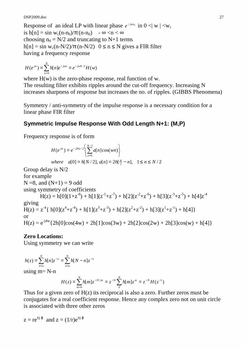
Symmetric Impulse Response With Odd Length N+1: (M, P)

Frequency response is of form

Group delay is N/2 for example N =8, and (N+1) = 9 odd using symmetry of coefficients

H(z) = h[0](1+z-8) + h[1](z-1+z-7) + h[2](z-2+z-6) + h[3](z-3+z-5) + h[4]z-4

giving H(z) = z-4 h[0](z4+z-4) + h[1](z3+z-3) + h[2](z2+z-2) + h[3](z1+z-1) + h[4] or H(z) = e-j4w2h[0]cos(4w) + 2h[1]cos(3w) + 2h[2]cos(2w) + 2h[3]cos(w) + h[4] Zero Locations: Using symmetry we can write

using m= N-n

Thus for a given zero of H(z) its reciprocal is also a zero. Further zeros must be conjugates for a real coefficient response. Hence any complex zero not on unit circle is associated with three other zeros z = re±j ϕ and z = (1/r)e±j ϕ

2/1],[2][],2/[]0[

)cos(][)(

2

2/

0

2/

NnnhnaNhawhere

wnnaeeH

N

N

n

jNwjw

≤≤−==

= ∑

=

−

∑∑=

−

=

− −==N

on

nN

on

n znNhznhzh ][][)(

)(][][)( 1

00

−−−

=

+− === ∑∑ zHzzmhzzmhzH NN

mNN

m

mN

)(][)( 2/

0

wHeenheH jwNN

n

jwnjw −

=

− ==∑

DSP2009.doc 28

for the zeros on the unit circle, its reciprocal is also the conjugate, so these zeros are a pair z = e±j ϕ A real zero pairs with its reciprocal z = σ and z = 1/σ Any zero at +1 or –1 is its own reciprocal and can appear only once.

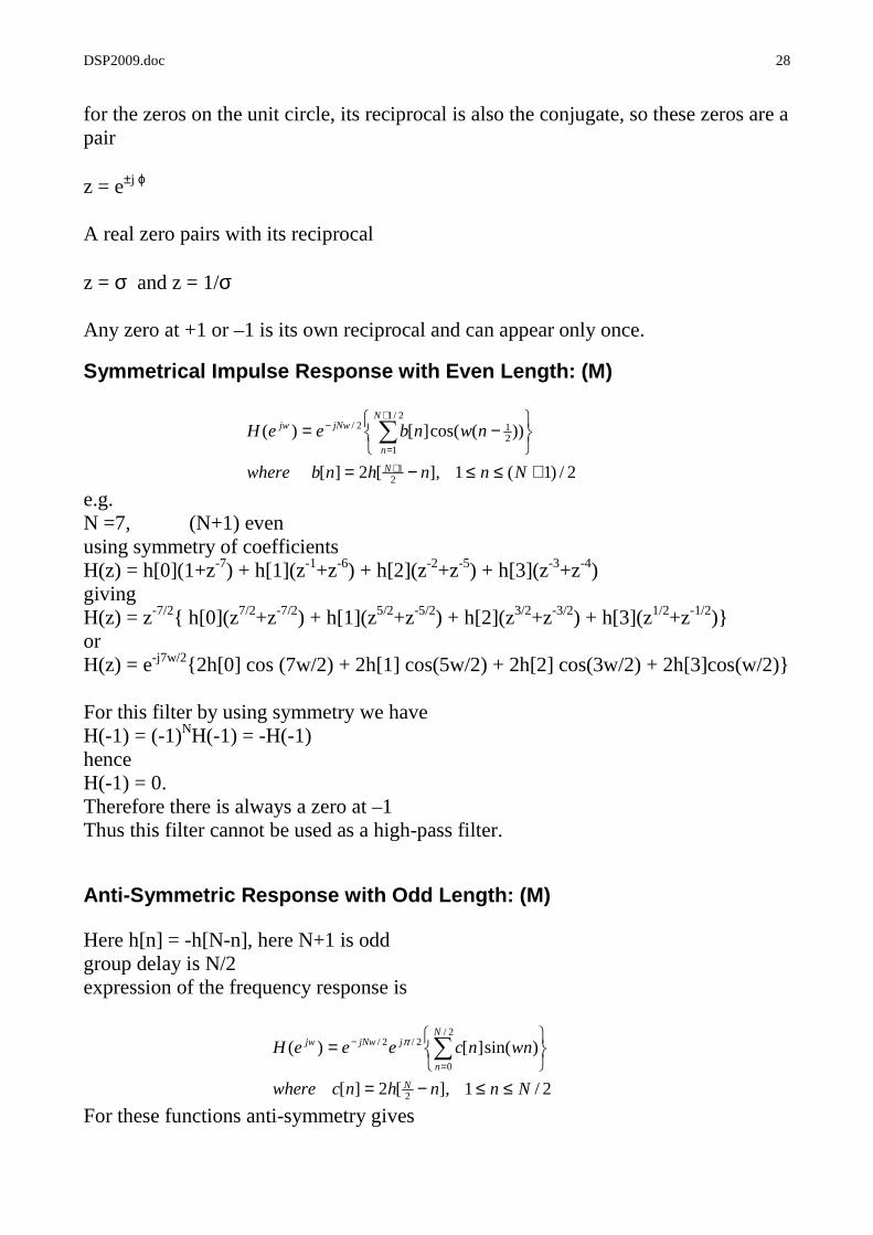
Symmetrical Impulse Response with Even Length: (M)

e.g. N =7, (N+1) even using symmetry of coefficients H(z) = h[0](1+z-7) + h[1](z-1+z-6) + h[2](z-2+z-5) + h[3](z-3+z-4) giving H(z) = z-7/2 h[0](z7/2+z-7/2) + h[1](z5/2+z-5/2) + h[2](z3/2+z-3/2) + h[3](z1/2+z-1/2) or H(z) = e-j7w/22h[0] cos (7w/2) + 2h[1] cos(5w/2) + 2h[2] cos(3w/2) + 2h[3]cos(w/2) For this filter by using symmetry we have H(-1) = (-1)NH(-1) = -H(-1) hence H(-1) = 0. Therefore there is always a zero at –1 Thus this filter cannot be used as a high-pass filter.

Anti-Symmetric Response with Odd Length: (M)

Here h[n] = -h[N-n], here N+1 is odd group delay is N/2 expression of the frequency response is

For these functions anti-symmetry gives

2/)1(1],[2][

))(cos(][)(

21

2/1

1212/

+≤≤−=

−=

+

+

=

− ∑

Nnnhnbwhere

nwnbeeH

N

N

n

jNwjw

2/1],[2][

)sin(][)(

2

2/

0

2/2/

Nnnhncwhere

wnnceeeH

N

N

n

jjNwjw

≤≤−=

= ∑

=

− π

DSP2009.doc 29

H(z) = -z-NH(z-1) Hence the poles are located as in the previous case and there is also a zero at z = -1 as H(-1) = -H(-1). Similarly there is a zero at +1 as H(1) = -H(1) It cannot be used in high-pass, Low-pass or Band-stop filters because of these zeros.

Anti Symmetric Response with Even Length: (M)

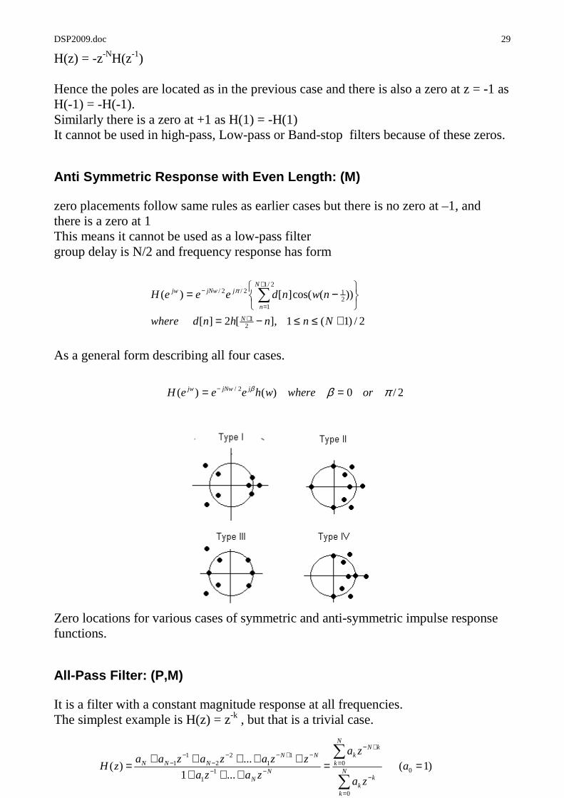
zero placements follow same rules as earlier cases but there is no zero at –1, and there is a zero at 1 This means it cannot be used as a low-pass filter group delay is N/2 and frequency response has form

As a general form describing all four cases.

Zero locations for various cases of symmetric and anti-symmetric impulse response functions.

All-Pass Filter: (P,M)

It is a filter with a constant magnitude response at all frequencies. The simplest example is H(z) = z-k , but that is a trivial case.

2/)1(1],[2][

))(cos(][)(

21

2/1

1212/2/

+≤≤−=

−=

+

+

=

− ∑

Nnnhndwhere

nwndeeeH

N

N

n

jjNwjw π

2/0)()( 2/ πββ orwherewheeeH jjNwjw == −

)1( ...1

...)( 0

0

01

1

11

22

11 ==

++++++++=

∑

∑

=

−

=

+−

−−

−+−−−

−− a

za

za

zaza

zzazazaazH N

k

kk

N

k

kNk

NN

NNNNN

DSP2009.doc 30

A system function of form is an all pass filter with ak real. If we define the denominator as A(z), with a0 = 1 then

and H(z)H(z-1) = 1= |H(z)|2, If z0 is a pole, then 1/z0 is a zero.

Phase function shows discontinuities of 2π which can be removed by UNWRAPPING. Properties: The All-pass function is a lossless bounded real transfer function. The magnitude of A(z)< 1 for z >1, = 1 for z = 1, > 1 for z <1 Unwrapped phase is monotonically decreasing so that group delay is positive. The change in the phase of the Mth order all-pass function as w goes from 0 to π radians is M π Application is as a delay equaliser. If G(z) is a filter designed to meet a given amplitude specification, its phase response will inn general be non-linear, It can then be cascaded with an all-pass filter A(z) such that the overall function has a linear phase and constant group delay

Stability:

Stability Triangle: (M,P)

If denominator in the H(z) is D(z) = 1 + d1z-1 + d2z

-2 In terms of its poles

D(z) = (1-λ 1z-1) (1-λ 2z

-1) = 1-(λ1+λ2)z-1 +λ1 λ2 z

-2 Thus d1 = -(λ1+λ2) and d2 = λ1 λ2 As poles are within unit circle, + λ1 < 1, λ2 < 1 hence d2 < 1 Also

)(

)()(

1

zA

zAzzH N

−−=

2

4 2211

2,1

ddd −±−=λ

DSP2009.doc 31

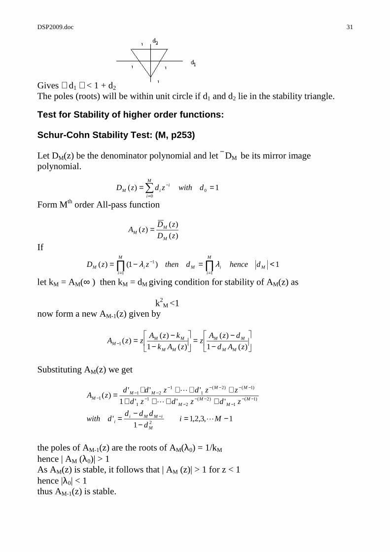
Gives d1 < 1 + d2

The poles (roots) will be within unit circle if d1 and d2 lie in the stability triangle.

Test for Stability of higher order functions:

Schur-Cohn Stability Test: (M, p253)

Let DM(z) be the denominator polynomial and let DM be its mirror image polynomial.

Form Mth order All-pass function

If

let kM = AM(∞ ) then kM = dM giving condition for stability of AM(z) as

k2M <1

now form a new AM-1(z) given by

Substituting AM(z) we get

the poles of AM-1(z) are the roots of AM(λ0) = 1/kM

hence | AM (λ0)| > 1 As AM(z) is stable, it follows that | AM (z)| > 1 for z < 1 hence |λ0| < 1 thus AM-1(z) is stable.

1)( 00

== −

=∑ dwithzdzD iM

iiM

)(

)()(

zD

zDzA

M

MM =

−−

=

−−

=− )(1

)(

)(1

)()(1 zAd

dzAz

zAk

kzAzzA

MM

MM

MM

MMM

1,3,2,11

'

'''1

''')(

2

)1(1

)2(2

11

)1()2(1

121

1

−=−

−=

++++++++

=

−

−−−

−−−

−

−−−−−−−

−

Mid

ddddwith

zdzdzd

zzdzddzA

M

iMMii

MM

MM

MMMM

M

L

L

L

1)1()(1

1

1

<=−= ∏∏=

−

=M

M

iiM

M

iiM dhencedthenzzD λλ

DSP2009.doc 32

We carry out this process for kM-2,….k1 then AM(z) is stable if Ki

2 < 1 for all i.

example: using

Hence system is stable.

Digital FIR Filter Design:

IIR and FIR selection:

• FIR can have linear phase response, are always stable if realised non-recursively, are affected less by quantisation and rounding errors

• IIR require less no. of coefficients. They are derivable using analog filter design techniques, and are easier to synthesise

• Therefore use IIR when requirement is for a sharp cut-off and high throughput • Use FIR if no . of coefficients is not too large, and if linear phase is required

Steps in Design of digital filters:

1. Give specifications and filter type 2. Select suitable method and calculate coefficients of the filter transfer function. 3. Convert transfer function into a suitable structure such as cascade realisation or

parallel realisation. 4. Analyse for error from finite bit number effects. 5. Implement by building hardware or software for actual filtering operation.

FIR filter design:

DSP2009.doc 33

FIR filter is characterised by a constant coefficient difference equation

where N is the filter length. It is a non-recursive all zero form and is always stable. This is a straightforward way to calculate the response. FIR filters can also be made to have an exactly linear phase response, with constant group and phase delays. Thus the filter is non-distorting. Finally FIR structures are easier to implement, and typical DSP processor architectures are suited to FIR filtering, the implementation results in less finite word-length errors.

Window method: (I,M)

Let the ideal filter be HD(w), then its impulse response is hD(n) which is obtained by inverse Fourier transform. Ideal impulse responses of the different filters are given below; LP:

n ≠ 0, with hD(0) = 2fc

HP:

n ≠ 0, with hD(0) =1- 2fc BP:

n ≠ 0, with hD(0) =2(f2-f1) BS:

n ≠ 0, with hD(0) =1-2(f2-f1) Ideal responses are infinite in duration, and decrease with increasing n. They are also symmetric, thus requiring calculation of only half the total number of coefficients. However, infinite duration implies infinite number of coefficients. Practical approach is to truncate the impulse response by setting hD(n) = 0 for n > say M. This is equivalent to multiplying hD(n) by a rectangular window w(n) = 1 , n = 0,1,…,M-1

∑−

=

−=1

0

)()(][N

k

knxkhny

c

ccD n

nfnh

ωω )sin(

2)( =

c

ccD n

nfnh

ωω )sin(

2)( −=

1

11

2

22

)sin(2

)sin(2)(

ωω

ωω

n

nf

n

nfnhD −=

2

22

1

11

)sin(2

)sin(2)(

ωω

ωω

n

nf

n

nfnhD −=

DSP2009.doc 34

= 0 elsewhere. In the frequency domain, this gives convolution of HD(w) and W(w), the latter having the (sin x)/x shape. The resulting impulse response of the windowed filter has ripples and overshoots in the pass and stop bands (Gibbs Phenomena). The transition width of the filter is greater, and depends on the width of the main lobe of the window function, and the ripples depend on the sidelobes. Instead of a rectangular window, other window functions may be used, which produce reduced ripples at the cost of greater transition width.

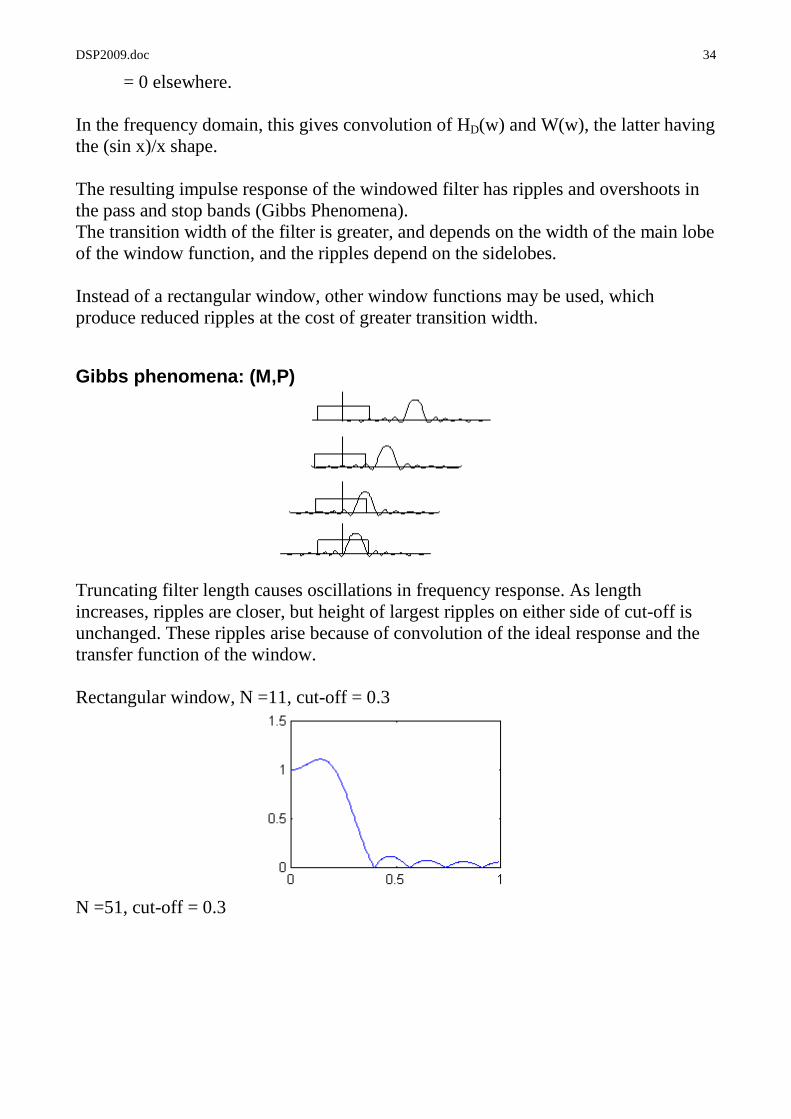
Gibbs phenomena: (M,P)

Truncating filter length causes oscillations in frequency response. As length increases, ripples are closer, but height of largest ripples on either side of cut-off is unchanged. These ripples arise because of convolution of the ideal response and the transfer function of the window. Rectangular window, N =11, cut-off = 0.3

N =51, cut-off = 0.3

DSP2009.doc 35

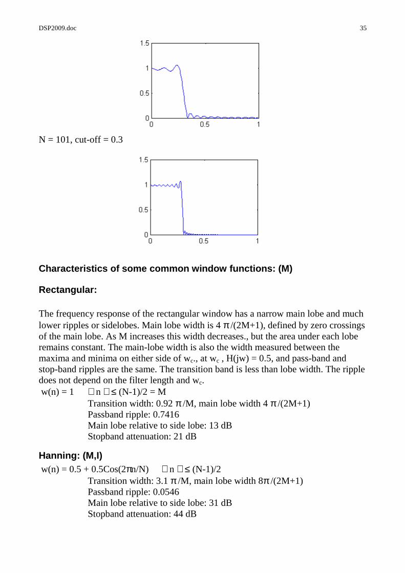
N = 101, cut-off = 0.3

Characteristics of some common window functions: (M )

Rectangular:

The frequency response of the rectangular window has a narrow main lobe and much lower ripples or sidelobes. Main lobe width is 4 π /(2M+1), defined by zero crossings of the main lobe. As M increases this width decreases., but the area under each lobe remains constant. The main-lobe width is also the width measured between the maxima and minima on either side of wc., at wc , H(jw) = 0.5, and pass-band and stop-band ripples are the same. The transition band is less than lobe width. The ripple does not depend on the filter length and wc. w(n) = 1 n ≤ (N-1)/2 = M Transition width: 0.92 π /M, main lobe width 4 π /(2M+1) Passband ripple: 0.7416 Main lobe relative to side lobe: 13 dB Stopband attenuation: 21 dB

Hanning: (M,I) w(n) = 0.5 + 0.5Cos(2πn/N) n ≤ (N-1)/2 Transition width: 3.1 π /M, main lobe width 8π /(2M+1) Passband ripple: 0.0546 Main lobe relative to side lobe: 31 dB Stopband attenuation: 44 dB

DSP2009.doc 36

Hamming: (M,I) w(n) = 0.54 + 0.46Cos(2πn/N) n ≤ (N-1)/2 Transition width: 3.3 π /M, main lobe width 8 π /(2M+1) Passband ripple: 0.0194 Main lobe relative to side lobe: 41 dB Stopband attenuation: 53 dB

Blackman: (M,I) w(n) = 0.42 + 0.5Cos(2πn/N-1) + 0.08 Cos(4πn/N-1) n ≤ (N-1)/2 Transition width: 5.5 π /M main lobe width 12π /(2M+1) Passband ripple: 0.0017 Main lobe relative to side lobe: 57 dB Stopband attenuation: 74 dB These windows have fixed characteristics, and equal Passband and Stopband ripples. This is their major disadvantage.

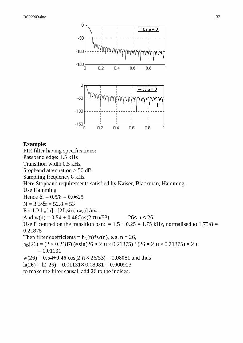
Kaiser window: (M,I) This window has a ripple control parameter β which allows adjustment of ripple against transition width. The window function is:

for -(N-1)/2 ≤ n ≤ (N-1)/2, and = 0 elsewhere. Here I0 is the zero-order modified Bessel’s function of the first kind., and β controls the way the function tapers at the edges in the time domain. With β = 0 Kaiser window corresponds to the rectangular window. With β = 5.44 results are very similar to the Hamming window. β is determined according to Stopband attenuation requirement as follows: if A ≤ 21 dB, β = 0 21 < A < 50 dB β = 0.5842(A-21)0.4 + 0.07886(A-21) A ≥ 50 dB β = 0.1102(A-8.7) where A = -20 log (δ ) and δ = min(δp, δs). The number of coefficients N is given by N ≥ (A-7.95)/14.36 ∆f where ∆f is the normalised transition width.

)(

12

1

)(0

2/12

0

β

β

I

N

nI

nw

−−

=

DSP2009.doc 37

Example: FIR filter having specifications: Passband edge: 1.5 kHz Transition width 0.5 kHz Stopband attenuation > 50 dB Sampling frequency 8 kHz Here Stopband requirements satisfied by Kaiser, Blackman, Hamming. Use Hamming Hence δf = 0.5/8 = 0.0625 N = 3.3/δf = 52.8 = 53 For LP hD[n]= [2fCsin(nwc)] /nwc And w(n) = 0.54 + 0.46Cos(2 π n/53) -26≤ n ≤ 26 Use fc centred on the transition band = 1.5 + 0.25 = 1.75 kHz, normalised to 1.75/8 = 0.21875 Then filter coefficients = hD(n)*w(n), e.g. n = 26, hD(26) = (2 × 0.21876)×sin(26 × 2 π × 0.21875) / (26 × 2 π × 0.21875) × 2 π = 0.01131 w(26) = 0.54+0.46 cos(2 π × 26/53) = 0.08081 and thus h(26) = h(-26) = 0.01131× 0.08081 = 0.000913 to make the filter causal, add 26 to the indices.

DSP2009.doc 38

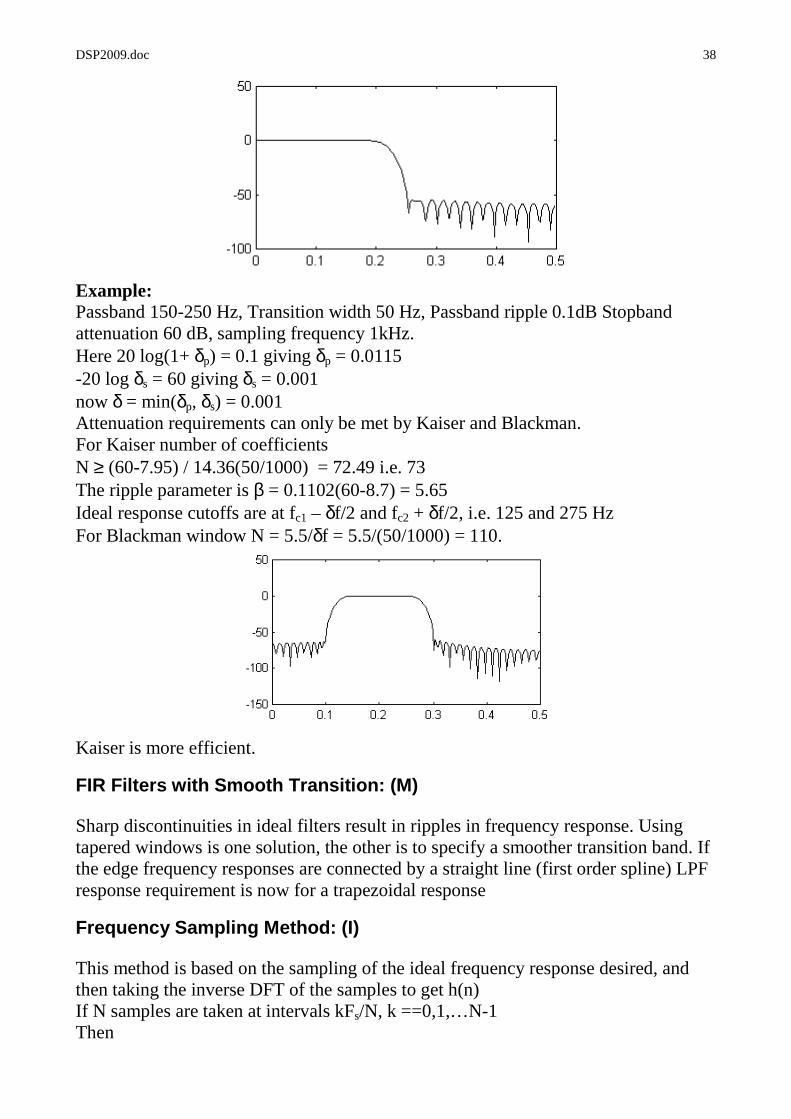
Example: Passband 150-250 Hz, Transition width 50 Hz, Passband ripple 0.1dB Stopband attenuation 60 dB, sampling frequency 1kHz. Here 20 log(1+ δp) = 0.1 giving δp = 0.0115 -20 log δs = 60 giving δs = 0.001 now δ = min(δp, δs) = 0.001 Attenuation requirements can only be met by Kaiser and Blackman. For Kaiser number of coefficients N ≥ (60-7.95) / 14.36(50/1000) = 72.49 i.e. 73 The ripple parameter is β = 0.1102(60-8.7) = 5.65 Ideal response cutoffs are at fc1 – δf/2 and fc2 + δf/2, i.e. 125 and 275 Hz For Blackman window N = 5.5/δf = 5.5/(50/1000) = 110.

Kaiser is more efficient.

FIR Filters with Smooth Transition: (M)

Sharp discontinuities in ideal filters result in ripples in frequency response. Using tapered windows is one solution, the other is to specify a smoother transition band. If the edge frequency responses are connected by a straight line (first order spline) LPF response requirement is now for a trapezoidal response

Frequency Sampling Method: (I)

This method is based on the sampling of the ideal frequency response desired, and then taking the inverse DFT of the samples to get h(n) If N samples are taken at intervals kFs/N, k ==0,1,…N-1 Then

DSP2009.doc 39

H(k) are the samples of the target frequency response.

where a = (N-1)/2

as h(n) is real. For a linear phase filter h(n) is symmetric leading to:

for N odd upper limit is (N-1)/2 Example:

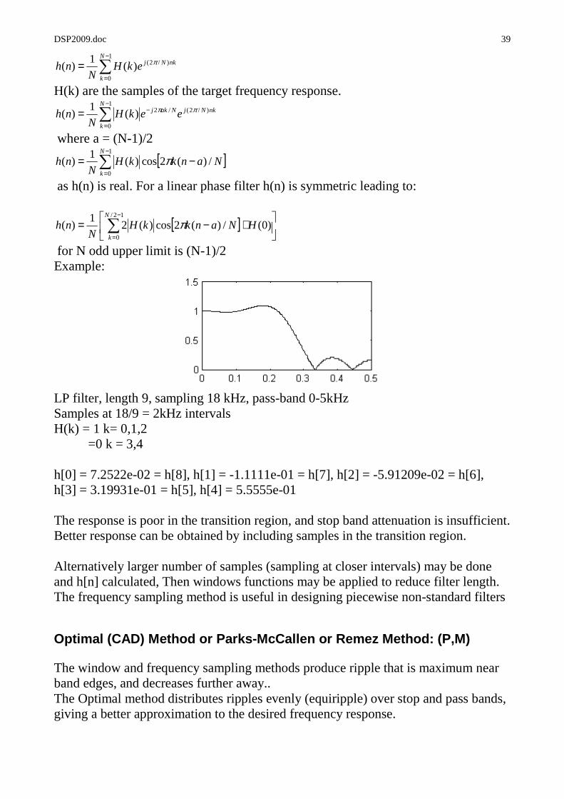
LP filter, length 9, sampling 18 kHz, pass-band 0-5kHz Samples at 18/9 = 2kHz intervals H(k) = 1 k= 0,1,2 =0 k = 3,4 h[0] = 7.2522e-02 = h[8], h[1] = -1.1111e-01 = h[7], h[2] = -5.91209e-02 = h[6], h[3] = 3.19931e-01 = h[5], h[4] = 5.5555e-01 The response is poor in the transition region, and stop band attenuation is insufficient. Better response can be obtained by including samples in the transition region. Alternatively larger number of samples (sampling at closer intervals) may be done and h[n] calculated, Then windows functions may be applied to reduce filter length. The frequency sampling method is useful in designing piecewise non-standard filters

Optimal (CAD) Method or Parks-McCallen or Remez Met hod: (P,M)

The window and frequency sampling methods produce ripple that is maximum near band edges, and decreases further away.. The Optimal method distributes ripples evenly (equiripple) over stop and pass bands, giving a better approximation to the desired frequency response.

∑−

=

=1

0

)/2()(1

)(N

k

nkNjekHN

nh π

∑−

=

−=1

0

)/2(/2)(1

)(N

k

nkNjNakj eekHN

nh ππ

[ ]∑−

=

−=1

0

/)(2cos)(1

)(N

k

NankkHN

nh π

[ ]

+−= ∑−

=

)0(/)(2cos)(21

)(12/

0

HNankkHN

nhN

k

π

DSP2009.doc 40

Let HD(w) be the ideal and H(w0 the actual and W(w) be a weighting function that allows the relative error of the approximation to be defined Then the difference between ideal and practical is E(w) = W(w)[HD(w) –H(w)] The method finds the h(n) which minimises the maximum weighted error in the pass and stop bands It can be shown that when max E(w) is minimised the filter will have an equi-ripple response, with the ripple alternating between two equal amplitude levels. (Alteration Theorem) for linear phase filters there are R+1 or R+2 such extremas, R = (N+1)/2. The locations of the extremal frequencies are generally not known except at the band edges fp and fs/2 If the extremal frequencies can be found, then the frequency response is known, and the impulse coefficients can be obtained. To find the extremal frequency the REMEZ algorithm (Parks-McCallen Algorithm) starts with an initial estimate of three R+1 extremas, and then uses a convergent iterative process to arrive at the extremal frequency values. The number of the extremal frequencies depends on the filter length, which can be calculated from the desired attenuation, ripple and transition band Example:

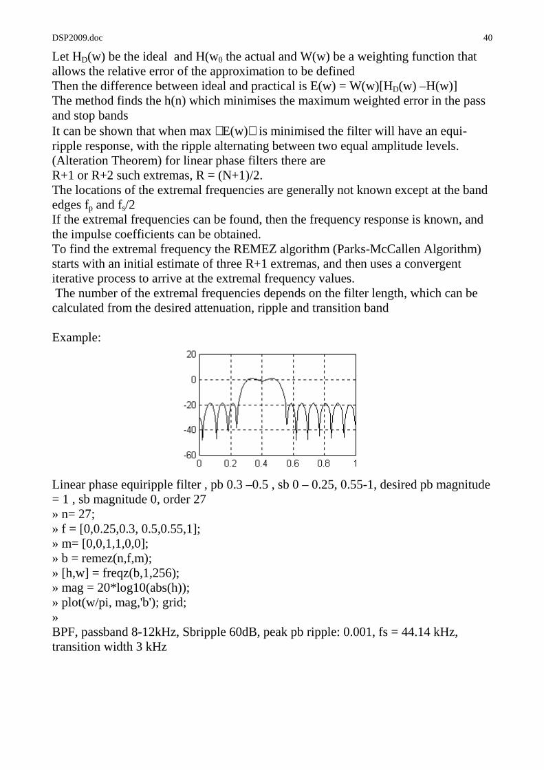
Linear phase equiripple filter , pb 0.3 –0.5 , sb 0 – 0.25, 0.55-1, desired pb magnitude = 1 , sb magnitude 0, order 27 » n= 27; » f = [0,0.25,0.3, 0.5,0.55,1]; » m= [0,0,1,1,0,0]; » b = remez(n,f,m); » [h,w] = freqz(b,1,256); » mag = 20*log10(abs(h)); » plot(w/pi, mag,'b'); grid; » BPF, passband 8-12kHz, Sbripple 60dB, peak pb ripple: 0.001, fs = 44.14 kHz, transition width 3 kHz

DSP2009.doc 41

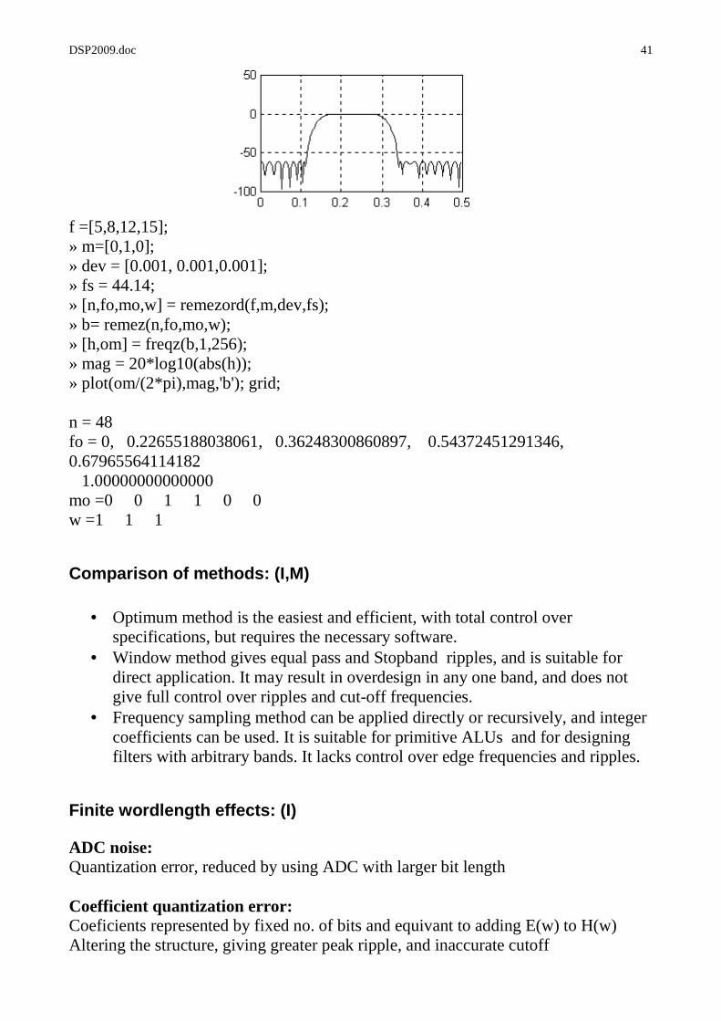
f =[5,8,12,15]; » m=[0,1,0]; » dev = [0.001, 0.001,0.001]; » fs = 44.14; » [n,fo,mo,w] = remezord(f,m,dev,fs); » b= remez(n,fo,mo,w); » [h,om] = freqz(b,1,256); » mag = 20*log10(abs(h)); » plot(om/(2*pi),mag,'b'); grid; n = 48 fo = 0, 0.22655188038061, 0.36248300860897, 0.54372451291346, 0.67965564114182 1.00000000000000 mo =0 0 1 1 0 0 w =1 1 1

Comparison of methods: (I,M)

• Optimum method is the easiest and efficient, with total control over specifications, but requires the necessary software.

• Window method gives equal pass and Stopband ripples, and is suitable for direct application. It may result in overdesign in any one band, and does not give full control over ripples and cut-off frequencies.

• Frequency sampling method can be applied directly or recursively, and integer coefficients can be used. It is suitable for primitive ALUs and for designing filters with arbitrary bands. It lacks control over edge frequencies and ripples.

Finite wordlength effects: (I)

ADC noise: Quantization error, reduced by using ADC with larger bit length Coefficient quantization error: Coeficients represented by fixed no. of bits and equivant to adding E(w) to H(w) Altering the structure, giving greater peak ripple, and inaccurate cutoff

DSP2009.doc 42

Roundoff error: x(n-m) is 12 bit and h(n) is 16 bit. The 24 bit product is rounded off to 16 bits in memeory, or 12 bit in DAC, may result in more severe effect than ADC quantisation. Avoided partly by using double length registers and rounding in the final step. Overflow error: When the sums exceed allowed wordlength. Avoided by scaling down h(n) and inputs by constants = sum of terms and then rescaling.

IIR Filter Design: (I, P,M)

IIR selection: • IIR require less no. of coefficients. They are derivable using analog filter

design techniques, and are easier to synthesise • Therefore Use IIR when requirement is for a sharp cut-off and high throughput

Steps in Design of digital IIR filters:

1. Give specifications and filter type 2. Select suitable lowpass analog filter prototype to meet the specifications. 3. Design the analog filter using specifications to find required order and

find prototype analog coefficients of the filter transfer function. 4. Use frequency band transformation (with pre-warping if necessary) to

convert the LP prototype to the required type of filter, and determine the equation of H(s).

5. Choose suitable analog to digital filter transformation method, and apply it to the analog filter to get the digital filter design.

6. Convert digital transfer function into a suitable structure such as cascade realisation or parallel realisation.

7. Analyse for error from finite bit number effects. If specifications are not met, repeat above steps choosing a higher order for the filter or different prototype.

8. Implement by building hardware or software for actual filtering operation.

Analog filter specifications: (M)

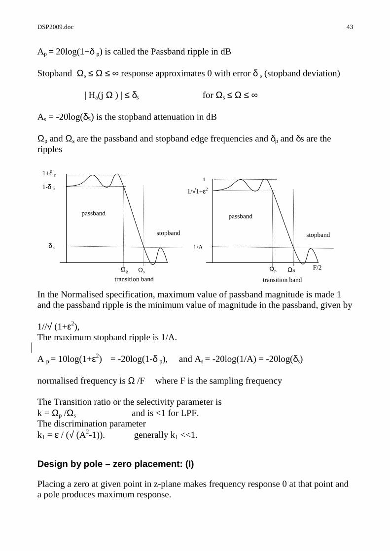
Ideal filters have brick-wall characteristics, which do not give causal impulse responses, and are therefore unrealisable. A realisable filter, say a LPF is generally specified by giving a desired passband gain of 1 with acceptable error (tolerance) ±δ p (Pass band deviation). 1-δp < | Ha(j Ω ) | <1+δp for | Ω | ≤ Ω p

DSP2009.doc 43

Ap = 20log(1+δ p) is called the Passband ripple in dB Stopband Ωs ≤ Ω ≤ ∞ response approximates 0 with error δ s (stopband deviation)

| Ha(j Ω ) | ≤ δs for Ωs ≤ Ω ≤ ∞

As = -20log(δS) is the stopband attenuation in dB Ωp and Ωs are the passband and stopband edge frequencies and δp and δs are the ripples

In the Normalised specification, maximum value of passband magnitude is made 1 and the passband ripple is the minimum value of magnitude in the passband, given by 1//√ (1+ε2), The maximum stopband ripple is 1/A. A p = 10log(1+ε2) = -20log(1-δ p), and As = -20log(1/A) = -20log(δs) normalised frequency is Ω /F where F is the sampling frequency The Transition ratio or the selectivity parameter is k = Ωp /Ωs and is <1 for LPF. The discrimination parameter k1 = ε / (√ (A2-1)). generally k1 <<1.

Design by pole – zero placement: (I)

Placing a zero at given point in z-plane makes frequency response 0 at that point and a pole produces maximum response.

transition band

passband

stopband

1

1/√1+ε2

1/A

Ωp Ωs

1+δ p

1-δ p

passband

stopband

transition band

δ s

Ωp Ωs F/2

DSP2009.doc 44

Poles close to unit circle give large peaks and zeros close to the circle produce troughs. For the coefficients to be real poles and zeros must be either real or in conjugate pairs. Further, poles must be within unit circle for stability For the pole with r > 0.9, bandwidth is approximately r = 1-(BW/F)π Example: Bandpass filter with complete rejection at 0 and 250 Hz, narrow passband centred at 125 Hz, and 3-dB bandwidth 10 Hz. Sampling frequency 500 Hz. zeros at 0 and 360 x 250/500 = 180 degrees. Pass band at 125 requires poles at ± 360 x 125/500 = ± 90 as conjugate pair. with BW = 10, F = 500, r = 0.937 for poles thus H(z) = (z-1)(z+1)/(z - 0.937ej π /2)(z - 0.937e-j π /2) i.e. H(z) = (1-z -2)/(1+0.877969z –2) The difference equation is y[n] = -0.877969y[n-2] + x[n] – x[n-2] Example 2 Notch filter, notch frequency 50 Hz, 3 dB BW ± 5Hz, sampling 500 Hz. To reject 50 Hz, a pair of complex zeros at ± 360 x 50/500 = ± 36 degrees To get sharp rejection a pair of poles at r < 1, from BW 10 Hz we get r = 0.938 The H(z) is H(z) = [z- e - j36][z- e j36]/ [z-0.937e –39.6] [z-0.937e +39.6] giving

Bilinear Transform Method Of IIR Filter Design: (P)

(For derivation of the bilinear transformation equation refer to Proakis and Manolakis) Bilinear transformation maps Left half s-plane uniquely into the unit circle in z-plane.

+−= −

−

1

1

1

12

z

z

Ts

0.937

]2[8780.0]1[5161.1]2[]1[6180.1][][

8780.05161.11

6180.11)(

21

21

−−−+−+−−=

+−+−= −−

−−

nynynxnxnxny

withzz

zzzH

DSP2009.doc 45

and an analog transfer function H(s) is mapped to the z plane as H(z) .

imaginary axis maps to unit circle, LHP to a point within the unit circle, and RHP to a point outside. Making substitution z = ejwT and s = jw’

s-plane w’ = k tan (wT/2), k = 1 or T/2 so +ve imaginary axis in s-plane is the upper half of unit circle. Similarly for the negative imaginary axis the lower half of the unit circle. This is a non-linear mapping and introduces a distortion called frequency warping. We therefore have to pre-warp the critical bandedge frequency to find their analog equivalents, design the analog prototype, using these pre-warped frequency and the transform with bilinear transform

In design the digital specifications are transformed to analogue by inverse bilinear transform, to get specifications of the analogue prototype. Then analogue filter is designed for the transformed specifications, Finally the bilinear transform is applied again to get the digital filter

jw’

σ

s-plane z-plane

Re z

Im z

1 -1

Bilinear transformation mapping

w

W’

π

-π

0

w’=k tan(wT/2)

+−= −

−=1

1

1

12)()(z

z

Ts

sHzH

DSP2009.doc 46

The process is summarised by: 1. Use digital specifications to decide upon a suitable normalised analogue transfer

function H(s) 2. Let the critical frequency of the digital filter be wp (cut-off or pass-band edge) 3. Obtain analogue critical frequency wp’ by pre-warping wp’ = k tan(wpT/2) 4. De-normalise the analogue filter replacing s with s/wp’ 5. Apply bilinear transformation replacing s by (z-1)/(z+1) Example: Normalised transfer function is H(s) = 1 / (s+1). Sampling frequency 150 Hz and cut-off 30 Hz Critical frequency is wp = 2 π 30 rad. analogue frequency after pre-warping wp’ = tan (wpT/2) with T = 1/150 we get wp’=0.7265 The de-normalised transfer function is H’(s) = 1/[(s / 0.7265) + 1] then H(z) = H’(s) with bilinear transform substitution H(z) = 0.4208 (1 + z –1) / (1-0.1584 z –1) The difference equation is y[n] = 0.1584y[n-1] + 0.4208[x[n] +x[n-1]]

Design using Analog filters:

Butterworth LPF: (I,P)

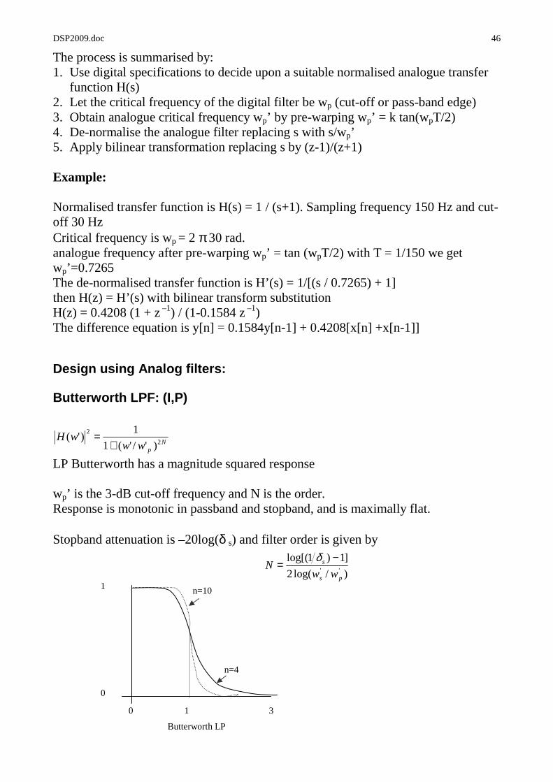
LP Butterworth has a magnitude squared response wp’ is the 3-dB cut-off frequency and N is the order. Response is monotonic in passband and stopband, and is maximally flat. Stopband attenuation is –20log(δ s) and filter order is given by

)/log(2

]1)1log[(''ps

s

wwN

−=

δ

1

0

0 3 1

Butterworth LP

n=4

n=10

Npww

wH2

2

)'/'(1

1)'(

+=

DSP2009.doc 47

The transfer function has zero at ∞ and uniformly spaced poles on a circle of radius wp’ in the s-plane These poles occur in conjugate pairs and lie on LHS of s-plans pk = wp’ e

j π (2k + N –1)/2N k = 1,2, …,N

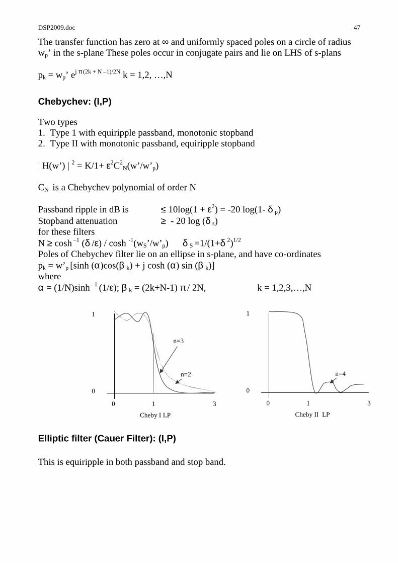
Chebychev: (I,P)

Two types 1. Type 1 with equiripple passband, monotonic stopband 2. Type II with monotonic passband, equiripple stopband | H(w’) | 2 = K/1+ ε2C2

N(w’/w’ p) CN is a Chebychev polynomial of order N Passband ripple in dB is ≤ 10log(1 + ε2) = -20 log(1- δ p) Stopband attenuation ≥ - 20 log (δ s) for these filters N ≥ cosh –1 (δ /ε) / cosh -1(wS’/w’ p) δ S =1/(1+δ 2)1/2 Poles of Chebychev filter lie on an ellipse in s-plane, and have co-ordinates pk = w’p [sinh (α)cos(β k) + j cosh (α) sin (β k)] where α = (1/N)sinh –1 (1/ε); β k = (2k+N-1) π / 2N, k = 1,2,3,…,N

Elliptic filter (Cauer Filter): (I,P) This is equiripple in both passband and stop band.

1

0

0 3 1

Cheby I LP

n=2

n=3

Cheby II LP

1

0

0 3 1

n=4

DSP2009.doc 48

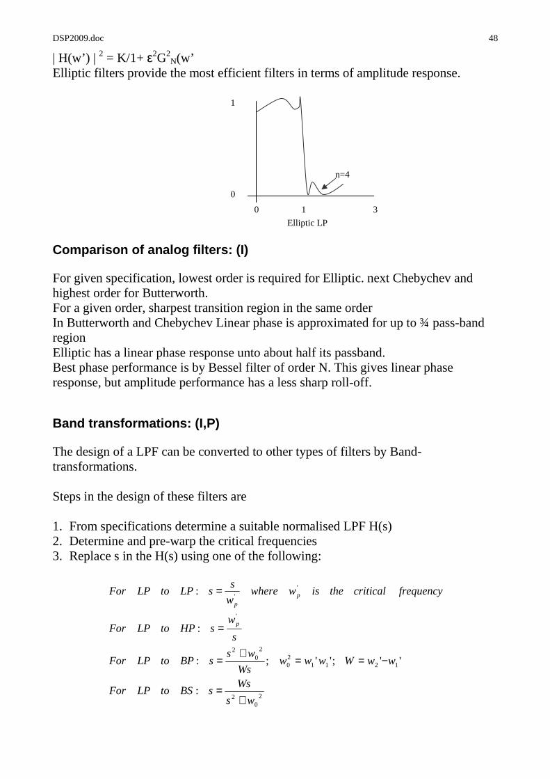
| H(w’) | 2 = K/1+ ε2G2N(w’

Elliptic filters provide the most efficient filters in terms of amplitude response.

Comparison of analog filters: (I)

For given specification, lowest order is required for Elliptic. next Chebychev and highest order for Butterworth. For a given order, sharpest transition region in the same order In Butterworth and Chebychev Linear phase is approximated for up to ¾ pass-band region Elliptic has a linear phase response unto about half its passband. Best phase performance is by Bessel filter of order N. This gives linear phase response, but amplitude performance has a less sharp roll-off.

Band transformations: (I,P)

The design of a LPF can be converted to other types of filters by Band-transformations. Steps in the design of these filters are 1. From specifications determine a suitable normalised LPF H(s) 2. Determine and pre-warp the critical frequencies 3. Replace s in the H(s) using one of the following:

1

0

0 3 1

Elliptic LP

n=4

20

2

121120

20

2

'

''

:

'';'';:

:

:

ws

WssBStoLPFor

wwWwwwWs

wssBPtoLPFor

s

wsHPtoLPFor

frequencycriticaltheiswwherew

ssLPtoLPFor

p

pp

+=

−==+

=

=

=

DSP2009.doc 49

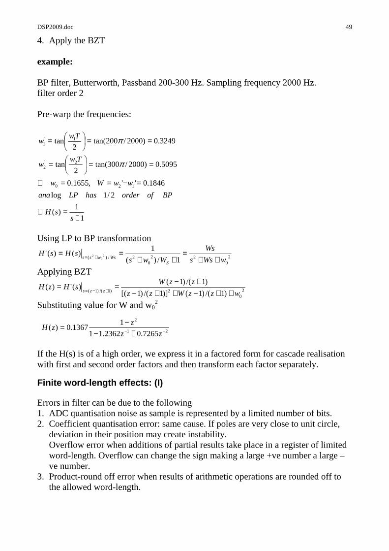
4. Apply the BZT example: BP filter, Butterworth, Passband 200-300 Hz. Sampling frequency 2000 Hz. filter order 2 Pre-warp the frequencies:

Using LP to BP transformation

Applying BZT

Substituting value for W and w02

If the H(s) is of a high order, we express it in a factored form for cascade realisation with first and second order factors and then transform each factor separately.

Finite word-length effects: (I)

Errors in filter can be due to the following 1. ADC quantisation noise as sample is represented by a limited number of bits. 2. Coefficient quantisation error: same cause. If poles are very close to unit circle,

deviation in their position may create instability. Overflow error when additions of partial results take place in a register of limited word-length. Overflow can change the sign making a large +ve number a large –ve number.

3. Product-round off error when results of arithmetic operations are rounded off to the allowed word-length.

1

1)(

2/1log

1846.0'',1655.0

5095.0)2000/300tan(2

tan

3249.0)2000/200tan(2

tan

120

2'2

1'1

+=∴

=−==∴

==

=

==

=

ssH

BPoforderhasLPana

wwWw

Tww

Tww

π

π

20

220

2/)( 1/)(

1)()(' 2

02

wWss

Ws

WwssHsH

SWswss ++

=++

==+=

20

2)1/()1( )1/()1()]1/()1[(

)1/()1()(')(

wzzWzz

zzWsHzH

zzs ++−++−+−==

+−=

21

2

7265.02362.11

11367.0)( −− +−

−=zz

zzH