Introduction: structural econometrics

Jean-Marc Robin

Abstract

1. Descriptive vs structural models

2. Correlation is not causality

a. Simultaneity

b. Heterogeneity

c. Selectivity

Descriptive models

Consider a sample of N observations of a couple of variables S = f(yi; xi); i = 1; :::; Ng.

A descriptive model is a statistical restriction (a list of assumptions) on the distribution of S.

It describes the statistical link between xi and yi, not the causal relationship between thesevariables.

Example: the linear model.

Assume xi 2 RK and X =

0BB@ xT1...

xTN

1CCA is full column rank (the columns of X are linearly indep.).

Then, the symmetric matrix XTX =PN

i=1 xixTi is invertible and the Ordinary Least Squares

(OLS) estimator exists:

bb = " NXi=1

xixTi

#�1 NXi=1

xiyi =�XTX

��1XTy where y =

0BB@ y1...

yN

1CCA :

1

Assuming moreover iid observations and E(xixTi ) non singular, the Law of Large Numbers impliesthat

plimN!1

bb = �E(xixTi )��1E(xiyi) � b:

Parameter b is the coe¢ cient of the theoretical regression of yi on xi. It describes the correlationsbetween yi and xi in the whole population whereas bb describes the correlations between yi and xiin the sample.bb and b always exist under these assumptions......even if the true Data Generating Process is not a linear model.

Examples: it may very well be that the true DGP is

� yi � N�cx2i ; �

2�, yi; xi 2 R.

� yi 2 f0; 1g and Pr fyi = 1jxig = ��xTi

�(Probit model).

2

Correlation is not causality

In general, however, correlations can be pointing in the wrong direction of causality.

This happens in particular

� when xi is endogenous: either because of simultaneity biases, or because of unobservedheterogeneity.

� when the sample is endogenous (selectivity biases).

3

Example of simultaneity bias:the supply-demand model

Aggregate demand: Di = a� bpi + ui.

Aggregate supply: Si = � + �pi + vi.

Assume demand shock ui and supply shock vi uncorrelated.

At the equilibrium, supply equals demand equals exchanged quantity:(yi = a� bpi + ui

yi = � + �pi + vi)

8><>:yi =

a� + b�

b + �+�ui + bvib + �

pi =a� �

b + �+ui � vib + �

:

Regressing yi on pi yields

=Cov (yi; pi)

Var (pi)=��2u � b�2v�2u + �

2v

which is a weighted average of b and �.

4

Instrumental variables

Demand curves and supply curves are identi�able if there exist observed supply and demand shocks:(ui = xTi c + "i

vi = zTi + �i

Under the assumptions that

Cov (xi; �i) = 0

Cov (zi; "i) = 0

� regressing yi on pi by Two Stage Least Squares (2SLS) using zi (supply shocks) to instrumentpi yields consistent estimates of a and b (demand curve);

� regressing yi on pi by Two Stage Least Squares (2SLS) using xi (demand shocks) to instrumentpi yields consistent estimates of � and � (supply curve).

5

Example of heterogeneity bias:convergence and growth

Do LDCs grow faster than developed countries so that their wealths will converge?

Idea: regress qit1 � qit0 on qit0 � qt0, for a sample f(qit0; qit1) ; i = 1; :::; Ng where qit is per capitaGDP (in log) of country i measured at two di¤erent times t0 and t1 (for example t0 = 1960 andt1 = 1990) and qt =

1N

PNi=1 qit.

The OLS estimate of b, bb, is found signi�cantly negative, which seems to imply that the countriesstarting from a high GDP value relative to the mean (qit0 � qt0 > 0) have a lower growth rate thanthe others.

Structural model.

Assume that the GDP of each country �uctuates around the same international trend but with

di¤erent levels:

qit = qt + �i + vit:

where E�i = 0 and Var�i = �2�, and vit is an iid shock, independent of �i and qt, with mean 0 andVar vit = �2v (white noise).

6

Regression to the mean 1

OLS estimator of the regression of qit1 � qt1 on qit0 � qt0:

b�10 = Pi

�qit1 � qt1

� �qit0 � qt0

�Pi

�qit0 � qt0

�2 =

Pi (�i + vit1) (�i + vit0)P

i (�i + vit0)2

P! Cov (�i + vit1; �i + vit0)

Var (�i + vit0)=

�2��2� + �

2v

= � < 1:

OLS estimator of the regression of qit0 � qt0 on qit1 � qt1:

b�01 = Pi

�qit0 � qt0

� �qit1 � qt1

�Pi

�qit1 � qt1

�2 =

Pi (�i + vit1) (�i + vit0)P

i (�i + vit1)2

P! Cov (�i + vit1; �i + vit0)

Var (�i + vit1)=

�2��2� + �

2v

= � < 1:

Hence the regressing qit1 � qt1 on qit0 � qt0 or qit0 � qt0 on qit1 � qt1 yields two estimatorsb�10 andb�01 which converge to the same value � < 1!!!!

7

Regression to the mean 2

Lastly,

qit1 � qt1 = b�10 �qit0 � qt0�+ bui

, qit1 � qit0 = qt1 � qt0 +�b�10 � 1�| {z }

=b<0

�qit0 � qt0

�+ bui:

So, one obtainsbb < 0 although all countries follow parallel GDP trajectories, which therefore cannotconverge!

This result is known since Galton (1822-1911) who observed that regressing the sizes of sons on thesizes of fathers or the sizes of fathers on the sizes of sons produced a coe¢ cient less than one. Thisis the �regression to the mean�phenomenon.

8

Alternative model

Construct a dynamic model of each country�s GDP with heterogeneous levels:

qit = �i + �qi;t�1 + vit; i = 1; :::; N; t = 1; :::; T:

If � < 1 and (vit) is stationary, each country tends to �uctuate around a speci�c target�i1�� as

qit � qi;t�1 = � (1� �)

�qi;t�1 �

�i1� �

�+ vit:

�Clubs�of convergence: countries with similar values of �i.

9

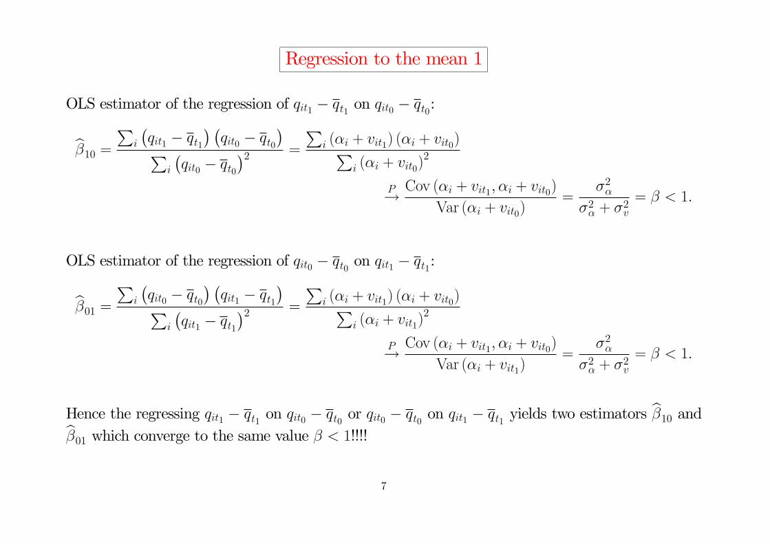
Example of selectivity bias:productivity and wages

Based on Heckman, Ecta, 1974.

I will develop the di¤erent steps from the construction of an economic model, to the constructionof the econometric model.

Individuals determine labour supply by trading o¤ consumption for leisure:

maxc;`

U(c; `) s.t.

(c = �h + �

0 < c; 0 < ` � T(1)

where utility function U(c; `) is increasing in consumption c and leisure `, � is the wage (equal tolabour productivity), � is nonlabour income.

Let

`�( �+=�

; � + �T�

) = argmaxc;`fU(c; `)jc + �` = �T + �; 0 < c; 0 < `g

be the Marshallian demand for leisure (interior solution to optimization programme, i.e. without

` � T ). The solution to (1) is

` (�; � + �T ) =

����� `� if `� < T

T if `� � T:

10

Proof

The Lagrangian is

L(c; `; 1; 2) = U(c; `) + 1(�T + �� c� �`) + 2(T � `);

where 1 and 2 are the Lagrange multipliers. A solution (c; `) is such that

@L(c; `; 1; 2)

@c=

@U(c; `)

@c� 1 = 0

@L(c; `; 1; 2)

@`=

@U(c; `)

@`� 1� � 2 = 0

with

2 � 0;

2(T � `) = 0;

c + �` = �T + �;

c > 0; T � ` > 0:

11

Interior solution. An interior solution, such that c > 0; T > ` > 0, has 2 = 0, and

@U(c; `)

@`/@U(c; `)

@c= �;

c + �` = �T + �:

Note that duality theory implies that the solution to this system is

` = `� (�; �T + �) = �@V (�; �T + �) =@�@V (�; �T + �) =@y

where

V (�; y) = maxc>0;`>0

U(c; `) s.t. c + �` = y;

is the indirect utility function associated to U .

12

Corner solution. A corner solution has ` = T; c = �, and

@U(�; T )

@`/@U(�; T )

@c= 1� + 2

1= � +

2 1� �:

as 1 > 0 as U(c; `) is strictly increasing wrt c. However, 2 can be equal to 0.

Lastly, by de�nition, `� (�; �T + �), satis�es

@U(c�; `�)

@`/@U(c

�; `�)

@c= �;

c� + �`� = �T + �:

The TMS @U(�(T�`)+�;`)@` /@U(�(T�`)+�;`)@c being a decreasing function (of `) when U is concave, the

inequality@U(�; T )

@`/@U(�; T )

@c� �

holds i¤ `� (�; �T + �) � T . (Draw a picture that shows that you want to be at the corner when`� (�; �T + �) � T .)

13

Speci�cation of labour supply function

The next step is to specify the labour supply functions.

First way. Choose a speci�cation for U or V and determine `.

Example:

V (�; y) = ����y +

�

�� ��

1� �� �2

2� �

�;

where y = �T + �. By Roy�s identity,

`� (�; y) = �@V (�; y)@�

/@V (�; y)@y

= �������1

hy + �

� ���1�� �

�2

2��

i+ ���

h� �1�� �

2 �2��

i���

= � + � +�

�+ �

y

�: (LS1)

14

Second way. Determine U or V such as ` has the desired form.

A good parametric speci�cation is linear:

`� (�; y) = �� � ln� + y; (LS2)

which is parametrically simpler as (LS1) (less parameters, e¤ects of � and y additively separable).

Is is possible to �nd a utility function which rationalizes this function?

Yes, one can show that

V (�; y) =

��� � ln�

+ y

�e� � � �

E1 ( �)

where E1 (t) =R1t

e�xx dx = �Ei (�t), works.

15

Proof

We search for a cost function y (�; v) such that V (�; y) = v and

�@V (�; y)@�

/@V (�; y)@y

= �� � ln� + y:

Fix v and di¤erentiate V (�; y) = v wrt �:

@V (�; y)

@�+@V (�; y)

@y

@y

@�= 0

or, assuming that @V (�;y)@y 6= 0,

@y (�; v)

@�= �� � ln� + y:

This is a linear ODE, the solution of which is easily found to be

y (�; v) = ��� � ln�

+

��

E1 ( �) + c (v)

�e �

where E1 (t) =R1t

e�xx dx = �Ei (�t) is the E1-exponential-integral function and c (v) is an arbi-

trary function of v, that has to be increasing for y (�; v) to be a cost function. Function c (v) isarbitrary, so one can take c (v) = v. By inverting y (�; v) = y wrt v, one proves the announcedresult.

16

Theoretical predictions

A model is useful if/as it allows to make predictions.

Consumer theory tells us that the cost function

y (�; v) = ��� � ln�

+

�v +

�

E1 ( �)

�e �

has to be increasing in v (true) and increasing and concave in �:

@y (�; v)

@�= �� � ln� + y (�; v) > 0;

@2y (�; v)

@�2= ��

�+

@y (�; v)

@�< 0:

Duality theory implies that @y(�;v)@� = `� (�; y (�; v)). Hence

`� (�; y) > 0 and � �

�+ `� (�; y) < 0:

These conditions cannot be imposed ex ante but should be veri�ed over the whole support of thedistribution of (�; y) after estimation.

Lastly, if leisure is a normal good,@`� (�; y)

@y= > 0:

Moreover, we see that ��� + `

� < 0 and `� > 0 imply that � > 0. Parameter � can be positiveor negative.

17

Econometric model

Now, we want to use the previous model to analyze a sample of individual data on female partici-pation. There is an iid sample of N observations of weekly hours worked (hi = T � `i), individualwage (wi)�if i does not work, then wi = �, the number of years of education (Edi), the individual�sage (Agei) and the husband�s wage (�i).

The theory yields the following model for (hi; wi):

hi

wi

!=

8>>>><>>>>:

h�i

�i

!if h�i > 0;

0

�

!if h�i � 0;

(selection rule)

where

h� (�; y) = T � `� (�; y) = T � � + � ln� � y:

An econometric model requires to consider themodelling of observed and unobserved heterogeneity.

18

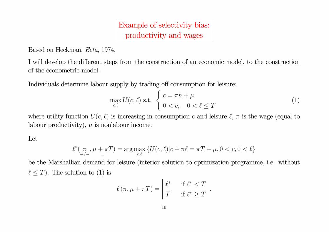
Modelling heterogeneity

We could assume that (h�i = aTxi + � ln�i + ui;

ln�i = bTzi + vi;(latent)

where

xi =�1; Edi; Expi; (Expi)

2 ; �i

�T; a = (a1; a2; a3; a4; a5);

zi =�1; Edi; Expi; (Expi)

2; Edi � Expi�T; b = (b1; b2; b3; b4; b5);

with Expi = Agei � Edi � 6, and ui

vi

!� N

0

0

!;

�2u ��u�v

��u�v �2v

!!:

The correlation between ui and vi re�ects omitted variables determining both individual preferencesand productivity.

Note that education and experience/age are likely to determine both preferences and productivity.

Note also that we have put some restrictions: �i only conditions preferences and the interactionEdi � Expi only conditions productivity. Always useful to have these sorts of restrictions as theyprovide instruments for potential endogeneity or selectivity problem.

19

Identi�cation

The next step is to discuss identi�cation.

Given that one has speci�ed a fully parametric model, parametric identi�cation is to show that twosets of parameters yielding the same likelihood value are necessarily equal.

Here, one can show that the selection model makes no di¤erence. The model is identi�ed if thelatent model (latent) is identi�ed. This requires the existence of variables determining ln�i but noth�i .

Nonparametric identi�cation holds when the distribution of observables picks only one set of para-meters irrespective of the stochastic assumption on the distribution of ui and vi.

Much more di¢ cult to prove. We shall come back to this point later.

20

Limited information models

In general it is useful to search for model parts which are simpler to estimate.

a. Participation model. Eliminate ln�i out of h�i :

h�i = aTxi + � ln�i + ui

= aTxi + �bTzi + ui + �vi

= cTqi + ri;

where

qi =�1; Edi; Expi; (Expi)

2 ; Edi � Expi; �i�T

;

c = (a1 + �b1; a2 + �b2; a3 + �b3; a4 + �b4; �b5; a5)T ;

ri = ui + �vi;

and vi

ri

!� N

0

0

!;

�2v �rv

�rv �2r

!!;

where �2r = �2u + �2�2v + 2���u�v and �rv = ��2v + ��u�v.

21

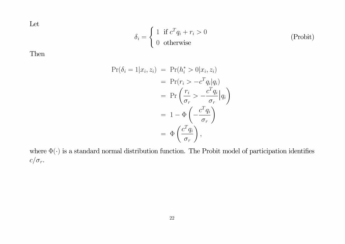
Let

�i =

(1 if cTqi + ri > 0

0 otherwise(Probit)

Then

Pr(�i = 1jxi; zi) = Pr(h�i > 0jxi; zi)= Pr(ri > �cTqijqi)

= Pr

�ri�r

> �cTqi�rjqi�

= 1� ���c

Tqi�r

�= �

�cTqi�r

�;

where �(�) is a standard normal distribution function. The Probit model of participation identi�esc=�r.

22

b. Reduced form labour supply model. Consider regressing hi on xi and zi using a TOBIT

model:

hi =

(cTqi + ri if cTqi + ri > 0

0 otherwise(Tobit)

This will separately identify c and �r.

c. Productivity equation. One has the following selection model for productivity:

lnwi =

(bTzi + vi if cTqi + ri > 0

� otherwise(Selection)

One can (should) use ML to estimate this selection model and consistently estimate b; c=�r; �v and�.

Alternatively, one can use Heckman�s two-step estimator:

E(ln�ijri; xi; zi) = bTzi + E (vijri; xi; zi)= bTzi + E (vijri)= bTzi +

�rv�2rri:

23

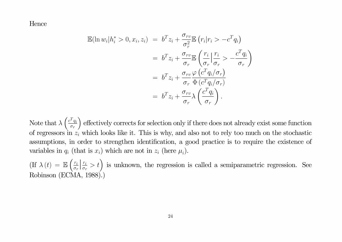
Hence

E(lnwijh�i > 0; xi; zi) = bTzi +�rv�2rE�rijri > �cTqi

�= bTzi +

�rv�rE�ri�rj ri�r

> �cTqi�r

�= bTzi +

�rv�r

'�cTqi=�r

�� (cTqi=�r)

= bTzi +�rv�r�

�cTqi�r

�:

Note that ��cT qi�r

�e¤ectively corrects for selection only if there does not already exist some function

of regressors in zi which looks like it. This is why, and also not to rely too much on the stochasticassumptions, in order to strengthen identi�cation, a good practice is to require the existence ofvariables in qi (that is xi) which are not in zi (here �i).

(If � (t) = E�ri�rj ri�r > t

�is unknown, the regression is called a semiparametric regression. See

Robinson (ECMA, 1988).)

24

Semiparametric regression

Consider the regression:

yi = xTi � + � (zi) + ui

Then

yi � E (yijxi) = � (zi)� E (� (zi) jxi) + ui � m (xi; zi) + ui

Function E (yijxi) is identi�ed, and so is m (xi; zi) = E [yi � E (yijxi) jxi; zi]. Hence:@m (x; z)

@z=d� (z)

dz

is identi�ed. So � (z) is identi�ed up to an additive constant.

For estimation, replace conditional expectations by conditional mean estimators, like the Nadaraya-

Watson kernel estimator:

x 7! bE (yijx) = NXi=1

yiK�xi�xh

�PNi=1K

�xi�xh

�whereK

�th

�is a function that puts a lot of weight at t = 0 et less and less when jtj gets away from

0 (like the density of a continuous distribution centered at 0).

25

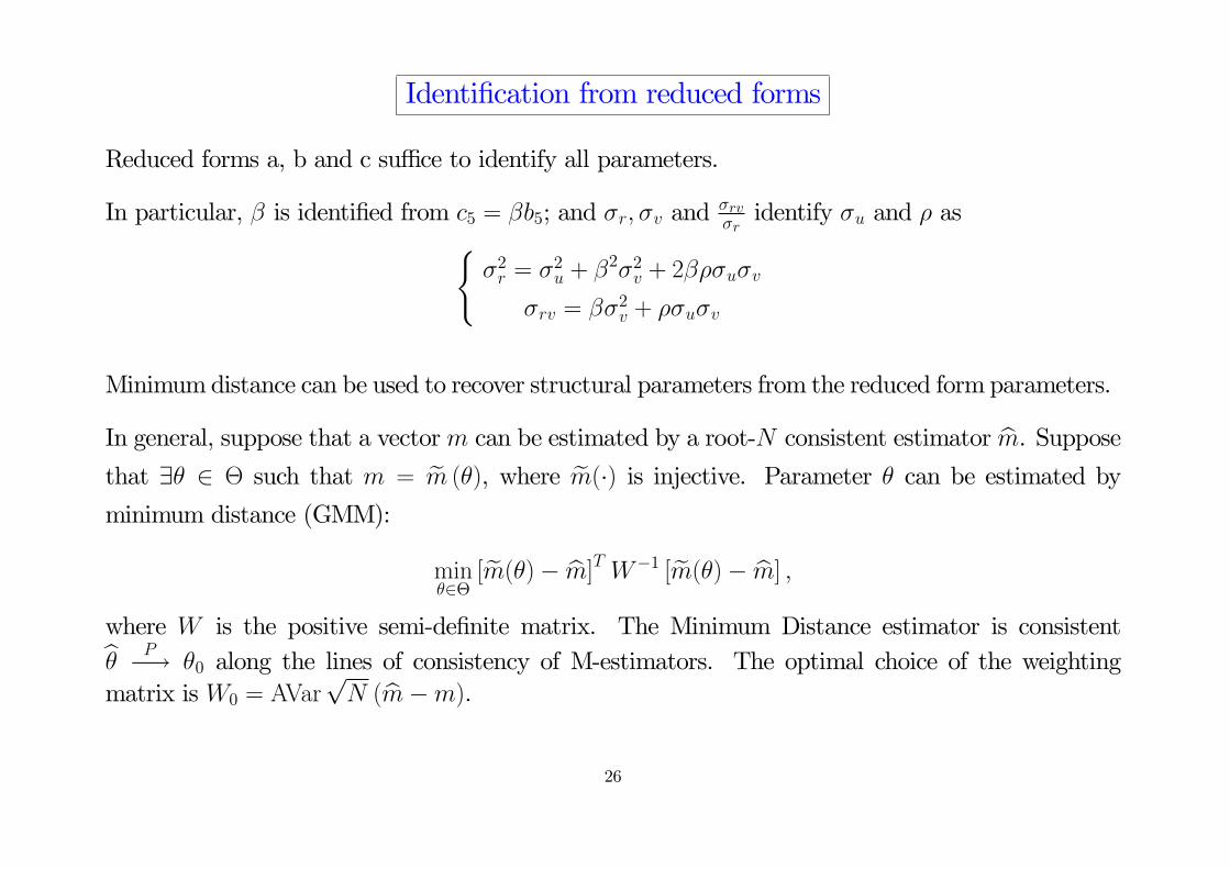
Identi�cation from reduced forms

Reduced forms a, b and c su¢ ce to identify all parameters.

In particular, � is identi�ed from c5 = �b5; and �r; �v and �rv�ridentify �u and � as(

�2r = �2u + �2�2v + 2���u�v

�rv = ��2v + ��u�v

Minimumdistance can be used to recover structural parameters from the reduced form parameters.

In general, suppose that a vectorm can be estimated by a root-N consistent estimator bm. Supposethat 9� 2 � such that m = em (�), where em(�) is injective. Parameter � can be estimated byminimum distance (GMM):

min�2�

[em(�)� bm]T W�1 [em(�)� bm] ;where W is the positive semi-de�nite matrix. The Minimum Distance estimator is consistentb� P�! �0 along the lines of consistency of M-estimators. The optimal choice of the weightingmatrix is W0 = AVar

pN (bm�m).

26

The asymptotic variance of the GMM estimator with the optimal weighting matrix is

AVar(b�) = �M0W�10 MT

0

��1N

;

where M0 =@ em(�0)@�T

.

In this example,

m =

�bT ; cT ;

�rv�r; �v; �r

�Tis related to

� =�aT ; �; bT ; �u; �v; �

�Tby the set of nonlinear equations sketched above.

27

Minimum distance

The MD estimator solves:

H�bm;b�� � @ em(b�)

@�TW�1

hem(b�)� bmi = 0:Taylor expansion in the neighboorhood of (m0 � em(�0); �0):

H�bm;b��| {z }=0

' H (m0; �0)| {z }=0

+@H (m0; �0)

@mT(bm�m0) +

@H (m0; �0)

@�T

�b� � �0

�, @H (m0; �0)

@�T

�b� � �0

�' �@H (m0; �0)

@mT(bm�m0)

where@H (m0; �0)

@�T=

@ em(�0)@�T

W�1�@ em(�0)@�T

�T�M0W

�1MT0

@H (m0; �0)

@mT= �@ em(�0)

@�TW�1 = �M0W

�1

If matrix M0W�1MT

0 (i.e. em(�) injective) is invertible, the consistency and asymptotic normalityof bm implies that of b�: p

N�b� � �0

�L! N (0;0 (W ))

28

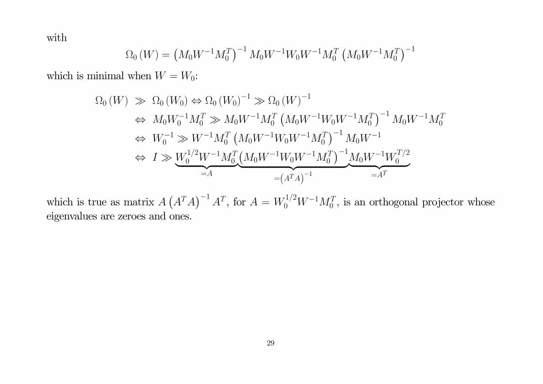
with

0 (W ) =�M0W

�1MT0

��1M0W

�1W0W�1MT

0

�M0W

�1MT0

��1which is minimal when W = W0:

0 (W ) � 0 (W0), 0 (W0)�1 � 0 (W )

�1

, M0W�10 MT

0 �M0W�1MT

0

�M0W

�1W0W�1MT

0

��1M0W

�1MT0

, W�10 � W�1MT

0

�M0W

�1W0W�1MT

0

��1M0W

�1

, I � W1=20 W�1MT

0| {z }=A

�M0W

�1W0W�1MT

0

��1| {z }=(ATA)

�1

M0W�1W

T=20| {z }

=AT

which is true as matrix A�ATA

��1AT , for A = W

1=20 W�1MT

0 , is an orthogonal projector whoseeigenvalues are zeroes and ones.

29

Full Maximum Likelihood

Full maximum likelihood yields e¢ ciency.

Usually, involves numerical optimization techniques. Reduced forms are useful to provide startingvalues for the algorithms and control the results (easy to make programming mistakes; Monte Carlosimulations recommended).

The likelihood is given by

L(�) =Yhi>0

pdf(ln�i = lnwi; h�i = hi)

Yhi=0

Pr(h�i � 0)

=Yhi>0

Pr(h�i = hij lnwi) pdf(ln�i = lnwi)Yhi=0

Pr(h�i � 0)

=Yhi>0

1

�up1� �2

'

aTxi + � ln�i +

��u�v�2v

�lnwi � bTzi

��up1� �2

!1

�v�

�ln�i � bTzi

�v

�Yhi=0

�1� �

�cTqi�r

��;

Notice that h�i = hi when hi > 0 implies that h�i > 0. So Pr (h�i > 0) is �embedded�in pdf(ln�i =

lnwi; h�i = hi).

30

Do not maximize L(�) directly. Operate �rst the change in variables:

a! a

�u; � ! �

�u; b! b

�v; �u !

1

�u; �v !

1

�v:

The likelihood becomes more linear in the parameters, which makes numerical convergence easierto achieve. Moreover, parameter � is usually di¢ cult to recover. It is advisable to use a grid searchfor �, i.e. maximize the likelihood wrt to a

�u; ��u ;

b�v; 1�u and

1�vfor di¤erent values of � in [�1; 1].

This provides a �rst approximation of b� and the other estimates. Then maximize the likelihoodwrt a

�u; ��u ;

b�v; 1�u ;

1�vand � starting from this point. This allows to �nd the right local maximum.

The MLE provides an e¢ cient estimator under the joint normality assumption. However, thejoint normality may be a strong assumption. Multi-step methods are often more robust as theyare consistent under less restrictive conditions. Moreover, the MLE is sometimes compositionallycumbersome.

31

Conclusion

It is very di¢ cult to properly analyze these issues of unobserved heterogeneity, simultaneity andselectivity without a proper economic model formatting the econometric equations.

Ideally, the econometric model should be the economic model. That is, heterogeneity and shocksshould be proper variables of the economic model, and the stochastic assumptions about theirdistributions should be embedded in the economic model itself.

I will call this empirical approach, structural econometrics.

Econometrics would then be only about the statistical techniques of inference on the model para-meters, not about modelling.

Unfortunately, this is not always the case. Papers start with a question. Then there is an economicinterpretation. Sometimes, a formal economic model is developed to analyze this questions, butnot always. Lastly, very often, a reduced form econometric study is provided which establishes afew correlations which are supposed to support the economic theory.

The aim of the remaining lectures is to study exemplary structural econometric papers.

32