Embed Size (px)
Citation preview

THE FEYNMAN PROPAGATOR ON PERTURBATIONS OF
MINKOWSKI SPACE
JESSE GELL-REDMAN, NICK HABER, AND ANDRAS VASY
Abstract. In this paper we analyze the Feynman wave equation on Lorentzianscattering spaces. We prove that the Feynman propagator exists as a map
between certain Banach spaces defined by decay and microlocal Sobolev reg-
ularity properties. We go on to show that certain nonlinear wave equationsarising in QFT are well-posed for small data in the Feynman setting.
1. Introduction
In this paper we use the method introduced in [43], extended in [2] and [24], toanalyze the Feynman propagator on spaces (M, g), called spaces with Lorentzianscattering metrics, that at infinity resemble Minkowski space in an appropriatemanner. As the Feynman propagator is of fundamental importance in quantumfield theory, we expect that our result and methods will be useful in a systematictreatment of QFT on curved, non-static, Lorentzian backgrounds.
Here the Feynman propagator is defined as the inverse of the wave operatoracting as a map between appropriate function spaces that generalize the behaviorof the standard Feynman propagator on exact Minkowski space. Thus, we set upfunction spaces which are weighted microlocal Sobolev spaces of an appropriate kindsuch that the wave operator for any Lorentzian scattering metric is Fredholm forall but a discrete set of weights – See Theorem 3.3 for a precise statement. Indeed,the same statement holds for more general perturbations of Lorentzian scatteringmetrics in the sense of smooth sections of Sym2 scT ∗M , defined below in Section 2.Further, for perturbations of Minkowski space, in the sense of smooth sections ofSym2 scT ∗M , we show in Theorem 3.6 that the operator is invertible for a suitablerange of weights, which is to say we prove the Feynman propagator exists for thesespace-times.
In order to give a rough idea for what the Feynman propagator is we recall thatin their groundbreaking paper [14] Duistermaat and Hormander constructed distin-guished parametrices for wave equations, i.e. distinguished solution operators for�u = f modulo C∞(M◦). Recall that by Hormander’s theorem [26], singularitiesof solutions of wave equations propagate along bicharacteristics inside the charac-teristic set in phase space, i.e. T ∗M◦; the projections of these to the base space arenull-geodesics. Here a bicharacteristic is an integral curve of the Hamilton vectorfield of the principal symbol of the wave operator, which is the dual metric functionon T ∗M◦. For the inhomogeneous wave equation, �u = f , if, say, f has wavefront set (i.e. is singular) at only one point in T ∗M◦, the different distinguishedparametrices produce solutions with different wave front sets, namely either the
The third author gratefully acknowledges partial support from the NSF under grant numberDMS-1068742 and DMS-1361432.
1

2 JESSE GELL-REDMAN, NICK HABER, AND ANDRAS VASY
forward or the backward bicharacteristic through the point in question. Here for-ward and backward are measured relative to the vector field whose integral curvesthey are, i.e. the Hamilton vector field. Note, however, that there is a differentnotion of forward and backward, which one may call future- or past-orientedness,namely whether the underlying time function is increasing or decreasing along theflow. The relative sign between these notions is the opposite in the two halves ofthe characteristic set of the wave operator over each point. We point out that fromthe perspective of microlocal analysis the natural direction of propagation is givenby the Hamilton flow.
As explained by Duistermaat and Hormander, a distinguished parametrix isobtained by choosing a direction of propagation (of singularities, or estimates)in each connected component of the characteristic set of the wave operator. Herethe direction of propagation is relative to the Hamilton flow, as above. If theunderlying manifold is connected, as one may assume, the characteristic set hastwo connected components, and there are 22 = 4 choices: propagation forwardrelative to the Hamilton flow everywhere, propagation backward along the Hamiltonflow everywhere (these are the Feynman and anti-Feynman propagators), resp.propagation in the future direction everywhere (the retarded propagator) and inthe past direction everywhere (the advanced propagator). A parametrix, however,is only an approximate inverse, modulo smoothing — smoothing operators are noteven compact on such a manifold; for actual applications (such as any computationsin physics) one would need an actual inverse, and most importantly a notion of aninverse. This is exactly what we provide in Theorem 3.6 below.
The historically usual setup for wave equations, and more generally evolutionequations, is that of Cauchy problems: one specifies initial data at a time slice, andthen one studies local or global solvability. In this sense wave equations are alwayslocally well-posed due to the finite speed of propagation, which in turn is proved byenergy estimates. Global well-posedness follows if the local solutions can be piecedtogether well: global hyperbolicity is a notion that allows one to do so. If one turnsthis into a setup of inhomogeneous wave equations, �u = f , by cutting f into twopieces, located in the future, resp. the past, of a Cauchy surface, the choice oneis making is that the support of u be in the future, resp. the past, of that of f .This necessarily implies, indeed is substantially stronger than, the statement thatsingularities of solutions are accordingly propagated, so two of the Duistermaat-Hormander parametrices correspond to these. Thus, due to the energy estimates,even when one considers global solutions, the Cauchy problem, or equivalentlythe future (or past) oriented problem, for the wave equation is essentially localin character, though, as discussed in [43, 24], in order to understand the globalbehavior of solutions, it is extremely useful to work directly in a global frameworkin any case.
What we achieve here is to give an analogous well-posedness framework for theFeynman problems (as opposed to the Cauchy problems). These problems are nec-essarily global in character, very much unlike the Cauchy problems. Thus, theybehave similarly, in a certain sense, to elliptic PDE. Indeed, from our perspec-tive, it is an accident (happening for good reasons) that the future/past orientedwave equations are local; one should not normally expect this for any PDE. To be
THE FEYNMAN PROPAGATOR ON PERTURBATIONS OF MINKOWSKI SPACE 3
more precise, singularities of solutions behave just as predicted by the Duistermaat-Hormander construction, but this has no content for C∞ solutions — the C∞ ‘part’of solutions is globally determined.
There has been extensive work in the mathematical physics literature on suchQFT problems, often from the perspective of trying to make sense of division byfunctions with zeros on the characteristic set: for Minkowski space, the Fouriertransform gives rise to a multiplier ξ2n− (ξ21 + . . .+ ξ2n−1); in a ±i0 sense division bythis is well-behaved away from the origin, but at the origin delicate questions arise.This is usually thought of as a degree of freedom in defining propagators: preciselyhow one extends the distribution to 0 even in this constant coefficient setting. (See[6, Section 5] for a discussion of this in the QFT context, and [45] for a recenttreatment of renormalization as such extensions.) From our perspective, this is dueto translational invariance of the problem being emphasized at the expense of itshomogeneity; Mellin transforming in the radial variable gives rise to a much betterbehaved problem. Indeed, a generalization of this is what Melrose’s framework of b-analysis [35] relies on; we further explore it here in the non-elliptic setting following[43, 24]. For the Feynman-type propagator then, i.e. where the microlocal structureof the function spaces the wave operator is acting on corresponds to the abovepropagation statements, the remaining choice is that of a weight: in the case ofMinkowski space it turns out that weights l with |l| < n−2
2 give rise to invertibility,while outside this range the index of the operator changes, with jumps at weightvalues corresponding to resonances of the Mellin transformed wave operator family,which in turn correspond to eigenvalues of the Laplacian on the sphere ∆Sn−1 aswe show by a complex scaling (Wick rotation) argument in Section 4.
For QFT on curved space-times, the work of Duistermaat and Hormander wasused to introduce a microlocal characterization of Hadamard states, which are con-sidered as physical states of non-interacting QFT, by Radzikowski [40]. (Indeed,part of the paper of Duistermaat and Hormander was motivated by QFT ques-tions.) This in turn was then extended by Brunetti, Fredenhagen and Kohler [5, 6].Gerard and Wrochna gave a new pseudodifferential construction of Hadamard states[16, 17]. In a different direction, Finster and Strohmaier extended the general the-ory to Maxwell fields [15]. However, in all these cases, there is no way of fixing apreferred state: one is always working modulo smoothing operators. Our frameworkon the other hand gives exactly such a preferred choice. Note also that the Feyn-man propagator we construct relates to an Hadamard-type condition; see Remark3.5 below.
In the settings with extra structure, involving time-like Killing vector fields, onecan construct Feynman propagators in terms of elliptic operators, e.g. via Cauchydata. Other constructions (such as extensions across null-infinity) in similar set-tings are investigated by Dappiaggi, Moretti and Pinamonti [11, 38, 12]. In fact,these latter results in bear the closest connections to ours in that a canonical stateis constructed using the structure on null-infinity. Our results deal directly withthe ‘bulk’, thanks to the Fredholm formulation, with the linear results having con-siderable perturbation stability in particular. (It is due to the module structurerequired in Section 5 that the non-linear problem is more restrictive.)
Along with setting up such a Fredholm framework, we also study semilinearwave equations, following the general scheme of [24]; we think of these as a firststep towards interacting QFT in this setting. However, being fully microlocal, the

4 JESSE GELL-REDMAN, NICK HABER, AND ANDRAS VASY
necessary framework requires more sophisticated function spaces than those dis-cussed in [24]. We prove small data well-posedness results in the Feynman settingfor certain semilinear wave equations in Theorems 5.11 and 5.16 below. In partic-ular, Theorem 5.16 can be summarized as follows
Theorem. In R3+1, if g is a perturbation of the Minkowski metric for which boththe invertibility statements in Theorem 3.6 and Theorem 5.1 hold, the problem
�u+ λu3 = f
is well-posed for small f , where f lies in the range, and u in the domain, of theFeynman wave operator, in particular u = �−1g,fey(f − λu3) where �−1g,fey is the
Feynman propagator mapping as in (3.18) with l ≥ 0 sufficiently small.
While as far as we are aware non-linear problems have not been considered inthe Feynman context, for the usual Cauchy problem, i.e. the retarded and advancedpropagators, non-linear problems on Minkowski space, as well as perturbations ofMinkowski space (as opposed to the more general Lorentzian scattering metricsconsidered in the linear parts of the paper here), have been very well studied.In particular, even quasilinear equations are well understood due to the work ofChristodoulou [8] and Klainerman [29, 28], with their book on the global stabilityof Einstein’s equation [9] being one of the main achievements. Lindblad and Rod-nianski [31, 32] simplified some of their arguments, and Bieri [3, 4] relaxed some ofthe decay conditions. We also mention the work of Wang [46] obtaining asymptoticexpansions, of Lindblad [30] for results on a class of quasilinear equations, and ofChrusciel and Leski [10] on improvements when there are no derivatives in the non-linearity. Hormander’s book [27] provides further references in the general area,while the work of Hintz and Vasy [24] develops the analogue of the framework weuse here in the general Lorentzian scattering metric setting (but still for the Cauchyproblem). Works for the linear problem with implications for non-linear ones, e.g.via Strichartz estimate include the recent work of Metcalfe and Tataru [37] wherea parametrix construction is presented in a low regularity setting.
The structure of the paper is as follows. In Section 2 we describe the underlyinggeometry and study the wave operator microlocally in the sense of smoothness (asopposed to decay). Estimates modulo compact errors, and thus Fredholm proper-ties, are established in Section 3. In Section 4 we show that in Minkowski space,the Feynman propagator is the limit of the inverses of elliptic problems, achievedby a ‘Wick rotation’; this means that from the perspective of spectral theory theFeynman and anti-Feynman propagators are the natural replacement for resolvents.This in particular establishes the invertibility of the Minkowski wave operator onthe appropriately weighted function spaces. Finally, in Section 5 we study semilin-ear wave equations in the Feynman framework.
The third author is grateful to Jan Derezinski, Christian Gerard and MichalWrochna for very helpful discussions, and the authors are grateful to Peter Hintzfor comments on the manuscript.
2. Geometry and the d’Alembertian
The basic object of interest is a manifold M with boundary ∂M equipped with aLorentzian metric g (which we take to be signature (1, n− 1)) in its interior whichhas a certain form at the boundary (which is geometrically infinity) modelled onthe Minkowski metric. In order to define the precise class of metrics, it is useful

THE FEYNMAN PROPAGATOR ON PERTURBATIONS OF MINKOWSKI SPACE 5
to introduce a more general structure. Thus, scT ∗M is the scattering cotangentbundle, which we describe presently, originally defined in [36]. If ρ is a boundarydefining function, meaning a function in C∞(M) which is non-negative, has {ρ =0} = ∂M , and such that dρ is non-vanishing on ∂M , smooth sections of scT ∗M nearthe boundary are locally given by C∞(M) linear combinations of the differentialforms
dρ
ρ2,
dwiρ,
where w1, . . . , wn−1 form local coordinates on ∂M . A non-degenerate smooth sec-tion of Sym2 scT ∗M of Lorentzian signature (which we take to be (1, n−1)) is calleda Lorentzian sc-metric. The smooth topology on sc-metrics is the C∞ topology onsections of scT ∗M . In order to make this class more concrete, the radial compacti-fication of Rn to a ball Bn, see [36], using ‘reciprocal spherical coordinates’ to gluethe sphere at infinity Sn−1 to Rn gives an example. Then C∞(Bn) consists exactlyof the space of classical (one step polyhomogeneous) symbols of order 0, while thestandard coordinate differentials dzj lift to Bn to give a basis, over C∞(Bn), of allsmooth sections of scT ∗Bn. In particular, any translation invariant Lorentzian met-ric on Rn is (after this identification) a sc-metric; and remains so under symbolicperturbations of its coefficients.
We next recall the definition of the more refined structure of a Lorentzian scat-tering space from [2] (see also [24, Section 5]), of which the Minkowski metric isan example via the radial compactification of Rn, depicted in Figure 2. For this,we assume that there is a C∞ function v defined near ∂M , with v|∂M having anon-degenerate differential at the zero-set S = {v = 0, ρ = 0} of v in ∂M (whichwe call the light cone at infinity); here ρ is a boundary defining function with theproperty that the scattering normal vector field V = ρ2∂ρ modulo ρVsc(M) (it iswell-defined in this sense) satisfies that g(V, V ) has the same sign as v at each pointin ∂M , g has the form
(2.1) g = vdρ2
ρ4−(dρ
ρ2⊗ α
ρ+α
ρ⊗ dρ
ρ2
)− g
ρ2,
where g ∈ C∞(M ; Sym2 T ∗M), α ∈ C∞(M ;T ∗M), α|S = 12 dv and g|Ann(dρ,dv) at
S is positive definite.This is not quite a statement about g|∂M as a metric on scTM , i.e. as a section of
Sym2 scT ∗M , because of the implied absence of a O(ρ)dρ2
ρ4 term. Adding such a term
results in a long-range Lorentzian scattering metric, the whole theory relevant to thediscussion below goes through in this setting, as shown in the work of Baskin, Vasyand Wunsch [1]; e.g. Schwarzschild space-time is of this form near the boundary ofthe light cone at infinity. (The difference is in the precise form of the asymptoticsof the linear waves; they are well-behaved on a logarithmically different blow-up ofM at S.)
Note that a perturbation of a Lorentzian scattering metric in the sense of sc-metrics (smooth sections of Sym2 scT ∗M) is a Lorentzian sc-metric, but it neednot be (even a long-range) Lorentzian scattering metric, since the above form ofthe metric (2.1) need not be preserved. However, the subspace of sc-metrics of theform (2.1) is a closed subset in the C∞ topology of sc-metrics within the open setof Lorentzian sc-metrics (in the space of smooth sections of Sym2 scT ∗M); by a
6 JESSE GELL-REDMAN, NICK HABER, AND ANDRAS VASY
perturbation in the sense of Lorentzian scattering metrics we mean a perturbationwithin this closed subset.
We remark here that, as is generally the case, only finite regularity (not beingC∞) is relevant in any of the discussion below, though the specific regularity neededwould be a priori rather high. However, using the low regularity results of Hintz[21] on b-pseudodifferential operators one could easily obtain rather precise low-regularity versions of the linear results presented here.
For statements beyond Fredholm properties, based on the work in Section 4, Mwill be the ball Bn, i.e. the radial compactification of Rn, equipped with a smoothperturbation of the Minkowski metric,
(2.2) g = dz2n − dz21 − dz22 − · · · − dz2n−1,
with perturbation understood in the set of sc-metrics. (Later, in Section 5, it will beimportant to have perturbations within scattering metrics to preserve the modulestructure discussed there.) To see that this takes the form in (2.1), following [2, Sect.3.1], set t = ρ−1 cos θ, zj = ρ−1ωj sin θ, where ρ = |z|, and ωj = zj/(ρ
2 − z2n)1/2.(Note that above we assumed that our boundary defining function was smooth onall of M , which our ρ here is certainly not; but we are only concerned about thevalue of ρ near the boundary, where we can take it to be the stated value with noproblem.) In this case α = dv/2 identically.
The main object of study here is the wave operator, defined in local coordinatesby
(2.3) �g :=1√g∂iG
ij√g∂j ,
where G denotes the inverse of g, i.e. the dual metric on 1−forms defined by g.We further assume that g is non-trapping, which is to say we assume that S =
S+ ∪S− (S± disjoint union of connected components), {ρ = 0, v > 0} = C+ ∪C−,C± open, ∂C± = S±, and such that the null-geodesics of g tend to S+ as theparameter goes to +∞, S− as the parameter goes to −∞, or vice versa. We thenconsider �g, on functions (or in the future differential forms or various other squaresof Dirac-type operators), and we wish to analyze the invertibility of the Feynmanpropagator. An important issue here is that �g is by no means self-adjoint on anynatural domain even though it is symmetric.
For this purpose it is convenient to conjugate �g and consider
(2.4) L = ρ−(n−2)/2ρ−2�gρ(n−2)/2;
then L ∈ Diff2b(M), the space of b-differential operators, meaning that locally
near ∂M , using coordinates (ρ, w1, . . . , wn−1) where ρ is the boundary definingfunction from (2.1) and wi are any coordinates on ∂M , there are smooth functionsai,α ∈ C∞(M), such that
L =∑
i+|α|≤2
ai,α(ρ∂ρ)i∂αw.
Its principal symbol is the dual metric G of the Lorentzian b-metric
(2.5) g = ρ2g.
In general, Diff∗b(M) is the algebra of differential operators generated by Vb, theset of smooth sections of bT (M), which more concretely is the C∞(M) span of the

THE FEYNMAN PROPAGATOR ON PERTURBATIONS OF MINKOWSKI SPACE 7
vector fields
(2.6) ρ∂ρ, ∂wi ,
That L is indeed in Diff2b(M) can be checked directly from (2.1) and (2.3). In
the definition of L in (2.4), ρ(n−2)/2 is introduced to make L formally self-adjointwith respect to the b-metric g. The conformal factor ρ merely reparameterizesnull-bicharacteristics, so our assumption is equivalent to the statement that null-bicharacteristics of L tend to S±,
One of the main features of our analysis, parallel to the recent work [24, 23] aswell as much other work on analysis on non-compact spaces going back to Melrose[35], is that we use an extension of the vector bundle T ∗(M int) up to the boundarywhich is better suited to the analysis than T ∗M , and for which in particular thebeginnings and ends of null-bicharacteristics become tractable objects. Concretely,we use the b-conormal bundle, bT ∗M , the dual bundle of the b-tangent bundlebTM , whose local sections near the boundary are C∞(M) linear combinations of
dρ
ρ, dwi,
coordinates as above. We describe the structure of the null-bicharacteristics at theboundary in detail now. The Hamilton flow on null-bicharacteristics correspondingto L descends from a flow on T ∗(M int) to a flow on the spherical cotangent bundleS∗(M int) := (T ∗(M int)− o)/R+ , where o denotes the zero section and the actionof R+ is the standard dilation action on the fibers. There is a natural map of the b-tangent space bTM −→ TM defined on sections, i.e. elements of Vb, by consideringa b-vector field as a standard vector field. (Thus the inclusion is not surjective overthe boundary.) We can use the dual map T ∗M −→ bT ∗M to define the b-conormalbundle of submanifolds; specifically, for our submanifold S, the conormal bundlebN∗S equal to the image in bT ∗M of covectors in T ∗M annihilating the image ofTS ⊂ TSM in bTM . It turns out that the null-bicharacteristics of L (see Figure2) terminate both at S+ and S− at the spherical b-conormal bundle
bSN∗S± = (bN∗S± \ o)/R+.
Before we describe this in more detail, we point out that bN∗S in fact has onedimensional fibers, since in coordinates ρ, v, si with ρ, v (so S = {ρ = 0 = v}) asabove and si local coordinates on S, so vectors in TS are ∂si , are annihilated byforms a dv+ b dρ in T ∗M , which map to forms a dv+ bρ(ρ−1 dρ) = a dv since S liesin the boundary ρ = 0. More concretely, the b-conormal bundle of S is generatedby dv. This means that
bSN∗S has two connected components.
Indeed, the flow on null-bicharacteristics, in view of the structure of the operatorat S±, as shown in [24, Section 5] makes the two halves of the spherical b-conormalbundle of S, bSN∗S = bSN∗+S ∪ bSN∗−S, into a family of sources (−) or sinks (+)
for the Hamilton flow, meaning that the null-bicharacteristics approach bSN∗+S+
as their parameter goes to +∞ and bSN∗−S− as the parameter goes to −∞, orbSN∗+S− as their parameter goes to +∞ and bSN∗−S+ as the parameter goes to
−∞. Correspondingly, the characteristic set Σ ⊂ bT ∗M \ o, which we also identifyas a subset of bS∗M , of L globally splits into the disjoint union Σ+ ∪ Σ−, withthe first class of bicharacteristics contained in Σ+, the second in Σ−. (The relevant

8 JESSE GELL-REDMAN, NICK HABER, AND ANDRAS VASY
S+
S−
C+
C−
ρ
hyperbolic
de Sitter
hyperbolic
v < 0
v > 0
v > 0
Figure 1. ρ equals zero exactly on the boundary and has non-vanishing differential there.
term in the dual metric is −4v∂2v , which gives 4(ξ′)2∂ξ′ for the Hamilton flow whereξ′ is dual to v, and this is a sink for infinity where ξ′ > 0 and a source for ξ′ < 0.)
Recall that the basic result for elliptic problems on compact manifolds withoutboundary is elliptic regularity estimates, which in turn imply Fredholm properties.Indeed, if P is an elliptic operator of order k on a compact manifold withoutboundary X, then for any m′ < m+ k one has the estimate
(2.7) ‖u‖Hm+k(X) ≤ C(‖Pu‖Hm(X) + ‖u‖Hm′ (X)).
That P is a Fredholm map from Hm+k(X) to Hm(X) is an immediate consequence
of this estimate and the fact that Hm+k(X) is a compact subspace of Hm′(X),together with the fact that P ∗, the formal adjoint of P , is then also elliptic, soanalogous estimates hold for P ∗.
Here we have real principal type points over M◦ as �g is non-elliptic, as well asso-called radial points at bSN∗±S±. Recall that real principal type estimates simplypropagate regularity along null-bicharacteristics, i.e. given that the estimate holdsat a point, one gets it elsewhere as well. The basic result at radial points which aresources or sinks, see [2, Proposition 4.4], [24, Proposition 5.1] and indeed [20] fora precursor in the boundaryless setting (in turn based on [43], which further goesback to [36]), in terms of b-Sobolev spaces, which we proceed to describe in detail, isthat subject to restrictions on the decay and regularity orders, in the high regularityregime, one has a real principal type estimate but without an assumption that onehas the regularity anywhere, provided one has at least a minimum amount of apriori regularity at the point in question. On the other hand, in the low regularitysetting, one can propagate estimates into the radial points, much as in the case ofreal principal type estimates. See Theorem 2.1.
To describe this concretely, we must first say what we mean precisely by regu-larity and vanishing order. For any manifold with boundary X, fix a non-vanishingb-density µ, i.e. a non-vanishing smooth section of the density bundle of bTX,which necessarily takes the form ρ−1µ for a non-vanishing density on the manifoldwith boundary X so in the coordinates ρ, v, y above is a smooth function times

THE FEYNMAN PROPAGATOR ON PERTURBATIONS OF MINKOWSKI SPACE 9
ρ−1 dρ dv dy, then letting
(2.8) 〈u, v〉L2b
=
∫X
uvµ,
define the weighted b-Sobolev spaces, first for integer orders k ∈ N by lettingu ∈ Hk
b (X) if and only if V 1 . . . V k′u ∈ L2
b for every k′−tuple of b-vector fieldsVi ∈ Vb with k′ ≤ k. For m ∈ R we have
Hmb (X) = {u ∈ C−∞(X) | Au ∈ L2
b(X) ∀A ∈ Ψmb (X)},
Hm,lb (X) = ρlHm
b (X)(2.9)
where Ψmb (X) is the space of b-pseudodifferential operators, described in Section
3. In general, we will allow a variable m ∈ C∞(bS∗X), in which case the rigorousdefinitions are below in (5.6)–(5.7). Note that we may choose the measure µ in
(2.8) so that H0,n/2b = L2 where L2 here and below denotes the standard Hilbert
space on Rn. Note that the L2b pairing gives an isomorphism
(2.10) (Hm,lb )∗ ' H−m,−lb .
For s ∈ R, the weighted b-Sobolev wavefront sets of a distribution u, denoted
WFs,lb (u) are the directions in phase space in which u fails to be in Hs,lb (X). A
concrete definition using explicit b-pseudodifferential operators is given in (3.9)
below, but for the moment we state that it is defined for u ∈ H−N,lb by
(2.11) WFs,lb (u) = ∩{
Σ(A) ⊂ bTX : Au ∈ Hs,lb (X)
},
where A ∈ Ψ0,0b (X), i.e. A is a (0, 0) order b-pseudodifferential operator (again, see
Section 3) and Σ(A) is the characteristic set (vanishing set of the principal symbol)
of A. Equivalently, a point (p, ξ) /∈ WFs,lb (u) (where ξ ∈ bT ∗pM \ o) if there exists
A ∈ Ψ0,0b (X) which is elliptic at (p, ξ) such that Au ∈ Hm,l
b (X). We say that u is
in Hs,lb microlocally if (p, ξ) 6∈ WFs,lb (u) where ξ ∈ bT ∗pM . There is a completely
analogous definition of WFm,lb for varying m ∈ C∞(bS∗X) and for l ∈ R.We have the following result, which is essentially [24, Proposition 5.1]. For the
following statement, let R be any of the above discussed connected components ofradial sets bSN∗±S±.
Proposition 2.1. Let (M, g) be a Lorentzian scattering space as in (2.1). Let L
be as above and u ∈ H−∞,lb (M).If m+l < 1
2 and m is nonincreasing along the Hamilton flow in the direction that
approaches R, then R is disjoint from WFm,lb (u) provided that R∩WFm−1,lb (Lu) =
∅ and a punctured neighborhood in Σ∩bS∗M of R with R removed is disjoint from
WFm,lb (u).On the other hand, suppose that m′ + l > 1
2 ,m ≥ m′ and m is nonincreasing
along the Hamilton flow in the direction that leaves R. Then if WFm′,l
b (u) and
WFm−1,lb (Lu) are both disjoint from R, then WFm,lb (u) is disjoint from R.
For elliptic regularity, the variable order m is completely arbitrary, for real prin-cipal type estimates in has to be non-increasing in the direction along the Hamiltonflow in which we wish to propagate the estimates.
So now fixing l and taking m satisfying m+ l > 1/2, resp. m+ l < 1/2 at exactlyone of bSN∗+S+, resp. bSN∗−S−, and similarly m + l > 1/2, resp. m + l < 1/2

10 JESSE GELL-REDMAN, NICK HABER, AND ANDRAS VASY
at exactly one of bSN∗−S+, resp. bSN∗+S−, we obtain Hm,lb estimates for u in
terms of Hm−1,lb estimates for Lu plus a weaker norm Hm′,l
b of u, m′ < m. To
make this precise we work with varying order Sobolev spaces Hm,lb (M). These
are discussed in detail in [2, Appendix] in the setting of standard Sobolev spaces(i.e. without the “b”), but since the development is nearly identical we discussthem only briefly. Specifically, given a function m ∈ C∞(bS∗M) that is monotonic
along the Hamilton flow, u ∈ Hm,lb (M) if and only if Au ∈ L2
b(M) for any A ∈Ψm,l
b = ρlΨmb , where for l = 0 membership of Ψm,l
b means that A is the quantization
of a symbol a ∈ C∞(bT ∗M) satisfying (among other standard symbol conditions
elaborated in [2, Appendix]) that |a(ρ, w, σ, ω)| ≤ C(1 + σ2 + |ω|2)m/2; here ρ isagain a boundary defining function, and coordinates on bT ∗M are obtained byparametrizing b-covectors as
σdρ
ρ+ ωidwi.
For l ∈ R, we thus have Hm,lb (M) := ρlHm,0
b (M); the norm on these spaces is given
by any elliptic A ∈ Ψm,lb together with the Hm′,l
b norm, where m′ < inf m. (This isonly defined up to equivalence of norms, but that is all we need.) Thus, given anys, r with s monotone along the Hamilton flow and r ∈ R, consider the spaces
(2.12) Ys,r = Hs,rb (M), X s,r = {u ∈ Hs,r
b (M) : Lu ∈ Hs−1,rb (M)}.
With m, l and m′ as above (in particular m is a function), we have the estimates
(2.13) ‖u‖Hm,lb (X) ≤ C(‖Lu‖Hm−1,lb (X) + ‖u‖
Hm′,l
b (X)).
(Here m′ < m can be taken to be a function, but this is not important. It can, forinstance, be taken to be an integer N < inf m.)
Note that the ‘end’ of the bicharacteristics at which m+ l < 1/2 is the directionin which the estimates are propagated, thus the choices
±(m+ l − 1/2) < 0 at bSN∗+S+, and
±(m+ l − 1/2) < 0 at bSN∗−S+
(2.14)
determine what (if any) type of inverse we get for L; we denote L on the corre-sponding spaces by L±± with the two ± corresponding to the two ± as in (2.14),i.e. the first to the direction of propagation in Σ+, the second to that in Σ−, withthe signs being positive if the propagation is towards S+. That is to say,
L±± denotes any map L : Xm,l −→ Ym−1,l
for which the pair (m, l) satisfy (2.14) with the given ±,± combination (the firstsign in the first inequality and the second in the second). Strictly speaking, L±±depends on m, but in fact we will see that the choice of m satisfying a particularversion of (2.14) is irrelevant. Thus we use the notation
(2.15) Xm,l±± = Xm,l for any (m, l) satisfying (2.14)
with the given ±, ± combination. See Figure 2.We call L++ the forward wave operator (corresponding to the forward solution),
L−− the backward wave operator, L+− and L−+ the Feynman wave operators, withL+− propagating forward along the Hamilton flow, and L−+ backward along theHamilton flow in both Σ+ and Σ−. Here we point out that either of the forward andbackward wave operators propagate estimates in the opposite directions relative to

THE FEYNMAN PROPAGATOR ON PERTURBATIONS OF MINKOWSKI SPACE 11
S+
bSN∗+S+,m+ l < 1/2
bSN∗−S+,m+ l > 1/2
S−
bSN∗−S−,m+ l > 1/2
bSN∗+S−,m+ l < 1/2
Figure 2. For the operator L+−, corresponding to the forwardFeynman problem, high regularity is imposed at the ‘beginning’(near bSN∗−S) of each null bicharacteristic, whether they begin atS+ or S−.
Σ+ Σ−
p p
S+
S−
p
Figure 3. The traces (i.e. projections from the cotangent space)of the light rays passing through an arbitrary point p. In the cotan-gent space these separate into the forward and backward pointingnull-bicharacteristics, depicted heuristically at right. The opera-tor L+− corresponds to propagation of singularities along the flow,and corresponds to the choice of + in the first and − in the secondinequality in (2.14)
the Hamilton flow in Σ+, resp. Σ−; the propagation is in the same direction relativeto a time function in the underlying space M .
3. Mapping properties of the Feynman propagator
The main result of this section is Theorem 3.3 below, which asserts that L±± areFredholm maps between appropriate Hilbert spaces. As mentioned, the estimatesin (2.13) are not sufficient to conclude that L is Fredholm, since the weaker normdoes not possess additional decay. Thus the main technical result of this sectionis the following. For (m, l) chosen as in (2.14) for any choice of signs ±±, and for

12 JESSE GELL-REDMAN, NICK HABER, AND ANDRAS VASY
certain choices of l (see the theorem), we have
‖u‖Hm,lb≤ C(‖Lu‖Hm−1,l
b+ ‖u‖
Hm′,l′
b
)
‖v‖H1−m,−lb
≤ C(‖Lv‖H−m,−lb+ ‖v‖
H1−m′′,−l′′b
)(3.1)
where m′ < m < m′′ and l′ < l < l′′. As explained in the proof of Theorem 3.3,
it is then a simple exercise using the fact that Hm,lb ⊂ Hm′,l′
b is compact providedm′ < m and l′ < l to show that L±± is Fredholm on the spaces in the theorem.
To obtain the improved estimates in (3.1), as in elliptic problems, we also need to
consider the Mellin transformed normal operator N(L)(σ) of L, which is a familyof differential operators on ∂M , parameterized by σ ∈ C. Given an arbitraryP ∈ Diff∗b of order k,
(3.2) P =∑
i+|α|≤k
ai,α(ρ, x)(ρ∂ρ)i∂αx ,
the normal operator is locally given by
(3.3) N(P ) :=∑
i+|α|≤k
ai,α(0, x)(ρ∂ρ)i∂αx ∈ Diffkb([0,∞)ρ × ∂M).
The Mellin transform is defined, initially on compactly supported smooth functionsu ∈ C∞(R+;C), by
M(u)(σ) = u(σ) =
∫ ∞0
ρ−iσu(ρ)dρ
ρ.
Note that Mu(σ) = Fv(σ) where F is the Fourier transform and v(x) = u(ex).Writing complex numbers σ = ξ + iη, it extends to a unitary isomorphism
(3.4) M : ρlL2(R+, dρ/ρ) −→ L2({Imσ = −l} , dξ).
The inverse map of (3.4) is given by
(3.5) M−1l f(ρ) =1
2π
∫{Imσ=−l}
ρiσf(ρ)dσ.
Moreover, composing N(P ) with the Mellin transform in ρ gives
(3.6) N(P )(σ) =∑
i+|α|≤k
ai,α(0, x)σi∂αx
We digress briefly to describe following typical example of a b-pseudodifferentialoperator which is elliptic at a point p ∈ bTM lying over the boundary, and how itrelates to the b-wavefront set discussed above. If p ∈ bT ∗M lies over the bound-ary, then some in coordinates (ρ, y, ξ, η) on bTM where ρ is a boundary definingfunction, ξ is dual to ρ and η to y, we have p = (0, y0, ξ0, η0). We obtain a b-pseudodifferential operator that is elliptic at p by choosing a cutoff function χ(ρ, y)with χ(0, y0) 6= 0 and such that χ is supported in {ρ < ε} for small ε, in particularsmall enough so that {ρ < ε} ' ∂M × [0, ε). Let φ(ξ, η) be a symbol, homogeneousnear infinity, non-zero in the cone given by positive multiples of (ξ0, η0). With Fthe Fourier transform in the y variables, we define
Au :=M−10 F−1φFM(χu).(3.7)

THE FEYNMAN PROPAGATOR ON PERTURBATIONS OF MINKOWSKI SPACE 13
Then A ∈ Ψ0,0b (M), and the b-principal symbol of A at order and weight (m, l) =
(0, 0) is:
(3.8) σ0,0(A) : bT ∗M −→ C, σ0,0(A) = χφ
where we think of χφ = χ(ρ, ξ)φ(ξ, η) as a function on bT ∗M , which near the bound-ary and with our coordinates is diffeomorphic to {ρ < ε, ξ} × T ∗∂M , supported onthe neighborhood of (0, y0, ξ0, η0) under consideration. In fact, such operators canbe used to neatly describe the b-wavefront sets of distributions. Given a distribution
u ∈ H−N,lb (M), then for m, l ∈ R,
(3.9) (0, y0, ξ0, η0) 6∈WFm,lb (u) ⇐⇒ ∃χ, φ with Aρ−lu ∈ Hm,0b (M),
where A is formed from χ and φ as in (3.7). (The ρ−l in the front is there so thatthe inverse Mellin transform M−10 of the resulting object is well defined.)
The structure and properties of N(L)(σ) are discussed at length in [24]. To
briefly summarize, for each σ, N(L)(σ) is a second order differential operator whichis elliptic in the interior of the regions C±, and hyperbolic on their complement
∂M \ (C+ ∪ C−) whose characteristic set splits into two components Σ±, each ofwhich contains a Lagrangian submanifold of radial points lying over S = ∂C+∪∂C−,and which split the conormal bundle N∗S (in ∂M) into four components N∗±S±which are sources (N∗−S) and sinks (N∗+S) for the Hamilton flow.
The estimates corresponding to those of the previous section allow one to con-clude that N(L)(σ) is Fredholm for each σ on the induced Sobolev spaces, whereImσ = −l, i.e. provided
±(m− Imσ − 1/2) < 0 at N∗+S+, and
±(m− Imσ − 1/2) < 0 at N∗−S+.(3.10)
More precisely here m is replaced by m|S∗∂MM , which is a well-defined subbundle ofbS∗∂MM . (The map T ∗M −→ bT ∗M discussed above restricts to the boundary togive a map from T ∗∂MM −→ bT ∗∂MM , from which one sees S∗∂MM as a subbundleof bS∗∂MM .) Thinking of σ as the b-dual variable of ρ (which thus depends on the
choice of dρρ at ∂M), covectors are of the form β+σ dρρ , β ∈ T ∗M , thus (identifying
functions on bS∗M with homogeneous degree 0 functions on bT ∗M \ o, where odenotes the zero section) for each σ 6= 0 one actually has a function on T ∗∂M .One thus obtains a family of large parameter norms (as described in the theoremjust below), analogous to the usual semiclassical norms: for σ in a compact set,the norms are uniformly equivalent to each other, but as σ →∞ this ceases to bethe case. In fact, we have the following applications of [2, Proposition 5.2], [43,Theorem 2.14].
Theorem 3.1. In strips in which Imσ is bounded, N(L)(σ)−1 has finitely manypoles.
Proof. As we will see momentarily, our family N(L)(σ) forms an analytic Fredholmfamily
(3.11) N(L)(σ) : Xm(∂M) −→ Ym−1(∂M),
where Xm(∂M) = {φ : φ ∈ Hm(∂M), N(L)(σ)φ ∈ Hm−1(∂M)}, and Ym(∂M) ={φ : φ ∈ Hm(∂M)} provided that σ and m are related as in (3.10), whose inverse
is thus meromorphic if N(L)(σ) is invertible for at least one σ = σ0. For bounded

14 JESSE GELL-REDMAN, NICK HABER, AND ANDRAS VASY
Imσ, we can see that N(L)(σ) is invertible for sufficiently large Reσ. This followsexactly as in [2, Proposition 5.2], which in turn follows directly from [43, Theorem2.14]. The key to this is to consider the semiclassical problem gotten by letting
h = |σ|−1 and z = σ|σ| , and, letting Pσ = N(L)(σ), studying
Ph,z := h2Ph−1z ∈ Ψ2h(∂M),
where Ψ2h(∂M) denotes the space of semiclassical pseudodifferential operators of
order 2 on ∂M . This semiclassical family on ∂M has Lagrangian submanifoldsof radial points (coming from the b-radial points of L), and, as described in [43,Section 2.8], the standard positive commutator proof of propagation of singularitiesaround Lagrangian submanifolds of radial points carries over to the semiclassicalregime without difficulty. This allows us to obtain estimates
‖u‖Hmh ≤ C(h−1‖Ph,zu‖Hm−1h
+ h‖u‖H−Nh )
‖v‖H1−mh≤ C(h−1‖Ph,zv‖H−mh + h‖u‖H−Nh )
for arbitrarily large N , within strips of bounded Imσ. As described at the be-ginning of the proof of Theorem 3.3 below, these estimates imply that N(L)(σ)mapping in (3.11) is Fredholm. Hence, for sufficiently small h, the −N norm canbe absorbed into the left hand side, giving by the first inequality injectivity and bythe second surjectivity. (This point is also elaborated in Theorem 3.3.) Note thatthe statement of [2, Proposition 5.2] is for only the forward and backward propa-gators, as the results come from microlocal positive commutator estimates whichare sufficiently microlocal, the conclusion, with the same proof, also holds for theFeynman operators. �
Remark 3.2. We point out that analogues of the estimates used so far go throughif L has sufficiently weak trapping with slight modifications: so-called b-normallyhyperbolic trapping, as introduced in [22], gives essentially the same estimates forσ real and large. (However, we do not study this here.)
Following [24] we will prove the following.
Theorem 3.3. Assume that (m, l) are chosen as in (2.14) for any choices ±,±,with the additional property that when the − sign is valid on the left hand side, i.e.−(m + l − 1/2) < 0, then in fact −(m + l − 3/2) < 0 as well, and such that there
are no poles of N(L)(σ)−1 on the line Imσ = −l, (where N(L) maps as in (3.11)with m = m|T∗∂M .) Then L is Fredholm as a map
(3.12) L : Xm,l → Ym−1,l.
In other words, if (m, l) are chosen to correspond to the signs ±± in (2.14), thenL±± is a Fredholm map for l satisfying the given condition on the poles.
Remark 3.4. Note that the Fredholm property is stable under b-perturbations ofL, in Ψ2,0
b . In particular, any perturbation of a Lorentzian scattering metric in thesense of sc-metrics gives rise to a similarly Fredholm problem.
Remark 3.5. Microlocal elliptic regularity states that WFm0,lb (u)\Σ ⊂WFm0−2,l
b (f)
if Lu = f and u ∈ Hm,lb for some m (i.e. u ∈ H−∞,lb ). Propagation of singularities,
in the sense of WFb, implies that if Lu = f , where u ∈ Hm,lb , f ∈ Hm−1,l
b for some
m, l satisfying (2.14) for the +− signs, then a point α ∈ Σ \ (bSN∗+S+ ∪ bSN∗+S−)

THE FEYNMAN PROPAGATOR ON PERTURBATIONS OF MINKOWSKI SPACE 15
(i.e. α is not at the radial sink, at which the function spaces have low regularity) is
not in WFm0,lb (u) provided that the backward bicharacteristic through α is disjoint
from WFm0−1,lb (f) and provided WFm0−1,l
b (f) is disjoint from bSN∗−S+∪bSN∗−S−,i.e. the radial sources at which high regularity is imposed. In particular, if f is
compactly supported in M◦, then WFm0,lb (u) \ (bSN∗+S+ ∪ bSN∗+S−) contained in
the order m0− 1 wavefront set of f together with the flowout of the intersection ofthe wavefront set of f with the characteristic set Σ of L. Restricted to the interior,where WFb is just the standard wave front set WF(u) ⊂ S∗M◦, this states that
(3.13) WFm0(u) ⊂WFm0−1(f)⋃
(∪t≥0Φt(WFm0−1(f) ∩ Σ))
where Φt is the time t Hamilton flow (on the cosphere bundle). In particular thisapplies to u = L−1+−f when L+− is actually invertible, so within the characteristicset the wave front set of u is a subset of the forward flowout of that of f .
There are analogous conclusions for the other choices of signs in (2.14) with thewavefront sets of solutions contained in the direction of the Hamilton flowout ofthe wavefront set of f corresponding to the choice of direction on each componentof the characteristic set. In particular, for the −+ sign, ∪t≥0Φt(WFm0−1(f) ∩ Σ)
is replaced by ∪t≤0Φt(WFm0−1(f) ∩ Σ).
Further, it is not hard to show that, provided L−1±± exists, the Schwartz kernel
K±± of L−1±± satisfies a corresponding wave front set conclusion in M◦ ×M◦. For
instance, for L−1+−, WF(K+−)\N∗diag is contained in the forward flowout ofN∗diag,the conormal bundle of the diagonal, with respect to the Hamilton vector field inthe left factor.
Proof. We wish to obtain the improvements to (2.13) in the estimates in (3.1).These estimates imply that the map in (3.12) is Fredholm. Indeed, using the fact
that the containment Hm,lb ⊂ Hm′,l′
b is compact provided m′ < m and l′ < l, thefirst estimate in (3.1) shows that the map has closed range and finite dimensionalkernel. Assuming that v lies in (image(L : Xm,l → Ym−1,l))⊥, where the orthogonal
complement is taken with respect to the L2b pairing (see (2.8)) between H1−m,−l
b
and Ym−1,l = Hm−1,lb , it follows that Lv = 0 and thus the second estimate in (3.1)
shows that the space of such v is finite dimensional.Thus we need only obtain the improved estimate in (3.1). The proof is essentially
the proof of [24, Proposition 2.3], and we recall it briefly for the convenience of the
reader. The condition on N(L)(σ)−1 on the line Im(σ) = −l implies by taking theinverse Mellin transform that the map
(3.14) N(L) : Xm′,l(∂M × R+) −→ Ym
′−1,l(∂M × R+)
is bounded and invertible, where m′ : T ∗∂M −→ R is any function satisfying theconstraints in (2.14) that m satisfies. Thus there is a C such that
‖u‖Hm′,l
b (∂M×R+)≤ C‖N(L)u‖
Hm′−1,l
b (∂M×R+),
and we may furthermore choose m′ so that it satisfies the constraint and thatm′ < m. Choosing a cutoff function χ that is supported near ∂M and equal to 1in a neighborhood thereof, we have (with a constant whose value changes from line

16 JESSE GELL-REDMAN, NICK HABER, AND ANDRAS VASY
to line)
‖u‖Hm,lb (M) ≤ C(‖Lu‖Hm−1,lb (M) + ‖u‖
Hm′,l
b (M))
≤ C(‖Lu‖Hm−1,lb (M) + ‖χu‖
Hm′,l
b (M)+ ‖(1− χ)u‖
Hm′,l
b (M))
≤ C(‖Lu‖Hm−1,lb (M) + ‖N(L)χu‖
Hm′−1,l
b (M)+ ‖u‖
Hm′,l′
b (M)).
Now, writing N(L)χ = [N(L), χ] + χ(N(L)− L) + χL, and using N(L)− L = ρPwhere P ∈ Diff2
b(M), and [N(L), χ] = ρP ′ where P ′ ∈ Diff1b(M), note that
‖u‖Hm,lb (M) ≤ C(‖Lu‖Hm−1,lb (M) + ‖u‖
Hm′+1,l′
b (M)),
so to obtain the improved estimate in (3.1) we need only make sure that m′+1 < mwhich can be done due to the −(m+ l− 3/2) < 0 assumption at appropriate radialsets. �
It is important to remark here that L±± are rather different operators for dif-ferent choices of ±±, on the other hand the choice of m, l satisfying the constraintscorresponding to a given ± (i.e. a given one of the two constraints) matter much
less: e.g. the invertibility of the normal operator N(L)(σ) is independent of theseadditional choices, so long as the m satisfies that m − Imσ − 1/2 has the correctsign at the relevant locations and has the correct monotonicity, in the Feynman casesee Proposition 4.7 below: the regularity theory shows that the potential kernel ofthe operator, as well as of the adjoint, is indeed independent of these choices. Thechoice of l does affect the index of L, however as a Fredholm operator, as we showfor the Feynman operator in Theorem 4.3.
We also note that the adjoint of L++ is L−−, while that of L+− is L−+, so oneshould not think of L as a self-adjoint operator even though it is of course formallyself-adjoint.
The standard setting in which �g is considered is that of evolutionary problems,
in which the forward or backward propagator L−1++ and L−1−− are considered. On theother hand, the Feynman propagator arises by Wick-rotating suitable Riemannianproblems. Here we are interested in the Feynman propagator, but we first explainthe more studied forward and backward problems in order to be able to contrastthese.
For the forward or backward problems the usual tools of evolutionary problems,namely standard energy estimates, can be used to compute the index in some cases,as discussed in [24, Theorem 5.2]. For this purpose it is useful to recall that for
the forward problem, the poles of N(L)(σ)−1 consist of resonances of the polesof the meromorphically continued resolvent RC+
(σ) (with Imσ > 0 the ‘physicalhalf plane’) and RC−(−σ) on the asymptotically hyperbolic caps C±, as well aspossibly a subset of iZ \ {0}. (The latter correspond to possible differentiateddelta distributional resonant states, which exist e.g. in even dimensional Minkowskispace and which are responsible for the strong Huygens principle on the one handand for the absence of poles of the meromorphically continued resolvent on odddimensional hyperbolic spaces on the other hand.) Further, the resonant statesand dual states have a certain support structure (this corresponds to C0 being
a hyperbolic region), namely for φ supported in C0 ∪ C+, N(L)(σ)−1φ can onlyhave poles if σ is either a pole of RC+
(σ) or is in −iN+, see [2, 44]. Thus, see[24], suppose that |l| < 1 (one could take l larger if one also excludes the possible
imaginary integer poles of N(L)(σ)−1), and RC±(σ) have no poles in Imσ ≥ −|l|,

THE FEYNMAN PROPAGATOR ON PERTURBATIONS OF MINKOWSKI SPACE 17
and that there is a boundary-defining function ρ which is globally time-like (in the
sense that dρρ is such with respect to g) near C+ ∪ C−. (These assumptions hold
e.g. on perturbations of Minkowski space.) Then any element of KerL would bevanishing to infinite order at C− (and the same for KerL∗, where L∗ is the adjointof L with respect to the L2
b = L2(Rn, µ) pairing in (2.8), with C− replaced by
C+) by the first hypothesis and vanishing in a neighborhood of C− by the second.Finally, a result of Geroch’s [18] (relying on a construction of Hawking’s) showsthat M is globally hyperbolic (there is a Cauchy surface for which every timelikecurve intersects it exactly one time) under these assumptions, and in particularL++ and L−− are invertible since any element of KerL++ would vanish globally,and similarly for elements of KerL∗++. One can then use the relative index theoremto compute the index on other weighted spaces.
For the Feynman propagator there is no simple direct identification of the polesof N(L)(σ). However, in Minkowski space, one can compute these exactly by virtueof a Wick rotation (Proposition 4.7), and further even show the invertibility of L
on appropriate weighted spaces (Theorem 3.6). Namely, the poles of N(L)(σ) areexactly those values of σ for which the operator ∆Sn−1 + (n − 2)2/4 + σ2 is not
invertible, i.e. σ is of the form ±i√λ+ (n− 2)2/4, λ an eigenvalue of ∆Sn−1 , i.e.
λ = k(k+n−2), k ∈ N, so λ+(n−2)2/4 = (k+(n−2)/2)2, and thus σ = ±i(n−22 +k).For future reference, we define
(3.15) Λ =
{±(n− 2
2+ k) : k ∈ N0
}This gives a gap between the two strings of poles with positive and negative imag-inary parts, and for |l| < n−2
2 , L+− and L−+ are invertible (and are adjoints ofeach other on dual spaces). Since the framework we set up is stable under generalb-ps.d.o. perturbations, we conclude that for general sc-metric perturbations g ofthe Minkowski metric g0, Lg,+− and Lg,−+ have the same properties, provided the|l| is taken slightly smaller:
Theorem 3.6. Let δ ∈ (0, n−22 ). Then there exists a neighborhood U of the
Minkowski metric g0 in C∞(M ; Sym2 scT ∗M) (i.e. in the sense of sc-metrics) suchthat for g ∈ U ,
(3.16) Lg,+− : Xm,l+− −→ Ym−1,l+−
is invertible for |l| < n−22 − δ and m satisfying the forward Feynman condition for
+− in (2.14), strengthened as in Theorem 3.3, and where Xm,l+− is the domain ofthe Feynman wave operator defined in (2.15). The same is true for Lg,−+ with +−replaced by −+ in all the spaces.
Proof. For the actual Minkowski metric g0, the invertibility is a restatement ofTheorem 4.6 below. Since the estimates in (3.1) hold uniformly on a sufficientlysmall neighborhood U ′ of g0, Lg,+− defines a continuous bounded family mappingas in (3.16), and thus is invertible on a possibly smaller neighborhood U . �
Taking into account the construction of L (see (2.4)), for metrics g in the neigh-borhood U in the theorem, we deduce that
(3.17) �g,+− : Xm,l+n−22
+− → Ym,l+n−22 +2
+−

18 JESSE GELL-REDMAN, NICK HABER, AND ANDRAS VASY
is invertible for |l| < n−22 −δ. Its inverse is indeed the forward Feynman propagator
(which is well defined on space Ym,l+n−22 +2
+− with weight l in the stated range,
(3.18) �−1g,fey : Ym,l+n−22
+− → Xm,l+n−22 +2
+− .
The same for +− replaced by −+ and “forward” replaced by “backward”.
Remark 3.7. The class of perturbations we consider does not preserve the radialpoint structure at bSN∗S±. Nonetheless, the estimates the radial point structureimplies for L and L∗ are preserved, much as discussed for Kerr-de Sitter spaces in[43].
4. Wick rotation (complex scaling)
In this section we work only with the Minkowski metric, which we continue todenote by g. We now explain Wick rotations in Minkowski space, where it amountsto replacing �g = D2
zn −D2z1 − . . .−D
2zn−1
by
(4.1) �g,θ = e−2θD2zn −D
2z1 − . . .−D
2zn−1
where θ is a complex parameter. Concretely, consider complex scaling, correspond-ing to pull-back by the diffeomorphism Φθ(z) = (z1, . . . , zn−1, e
θzn) for θ ∈ R, i.e.considering U∗θ�(U−1θ )∗, where Uθ = (detDΦθ)
1/2Φ∗θf , extending the result to ananalytic family of operators in θ ∈ C (near the reals). This gives rise to the family�g,θ. Letting
(4.2) Lθ = ρ−(n−2)/2ρ−2�g,θρ(n−2)/2,
as soon as Im θ ∈ (−π, π) \ {0}, Lθ is a an elliptic b-differential operator; whenθ = ±iπ/2, one obtains the Euclidean Laplacian �g,±iπ/2 = ∆Rn . In the ellipticregion the corresponding operator Lθ satisfies the Fredholm estimates uniformlyfor Lθ,+− (and its adjoint, for which the imaginary part switches sign, but onepropagates estimates backwards) when Im θ ≥ 0, and for Lθ,−+ when Im θ ≤ 0.
The main analytic property that we will use below for the operators Lθ is that forregularity functions m chosen to satisfy say the forward (+−) Feynman condition,the corresponding operators Lθ,+− satisfy estimates
(4.3) ‖u‖Hm,lb≤ C(‖Lθu‖Hm−1,l
b+ ‖u‖
Hm′,l′
b
).
uniformly in θ for m, l corresponding to +− and m′ < m, l′ < l, meaning precisely
that there is a constant C such that for |θ| < δ0, Im θ ≥ 0 for u ∈ Hm,lb , (4.3)
holds provided m, l satisfy the +− Feynman condition and −l 6∈ Λ. For |θ| <δ0, Im θ ≤ 0 they hold provided m, l satisfy the −+ Feynman condition and l 6∈ Λ.(Note that Λ = −Λ so actually the conditions on l are the same.) The reasonfor the uniformity is that all of the ingredients are uniform; this is standard forelliptic estimates. On the other hand, it holds for real principal type estimateswhere the imaginary part of the principal symbol amounts to complex absorption,provided one propagates estimates in the forward direction of the Hamilton flow ifthe imaginary part of the principal symbol is ≤ 0 (which is the case for Im θ ≥ 0, θsmall) and backwards along the Hamilton flow if the imaginary part of the principalsymbol is ≥ 0, as shown by Nonnenmacher and Zworski [39] and Datchev and Vasy[13] in the semiclassical microlocal setting and, as is directly relevant here, extendedto the general b-setting by Hintz and Vasy [24, Section 2.1.2]. Moreover, at radial

THE FEYNMAN PROPAGATOR ON PERTURBATIONS OF MINKOWSKI SPACE 19
points in the standard microlocal setting this was shown by Haber and Vasy [20],and the proof of Proposition 2.1 can be easily modified in the same manner sothat non-real principal symbol is also allowed at the b-radial points. Finally, thenormal operator constructions are also uniform since they rely on estimates for theMellin transformed family which are uniform as we stated; the resonances (poles)of the inverse of this family thus a priori vary continuously, so in particular nearan invertible weight for θ = 0 one has uniform estimates. (In fact we will showin Proposition 4.7 below that the poles of the complex scaled normal families areconstant, i.e. do not vary with θ.)
Note that the estimates in (4.3) are not the standard elliptic estimates. Indeed,the term on the left hand side is in a space of differentiability order one lower thanellipticity provides. The point is that the estimates in (4.3) are exactly those whichare uniform down to Im θ = 0.
The family of operators Lθ defines a family of Mellin transformed normal op-erators on the boundary, N(Lθ)(σ) as above, and we have, still for g equal to theMinkowski metric, that
(4.4) N(L±iπ/2)(σ) = ∆Sn−1 + (n− 2)2/4 + σ2.
We recall the theorem of Melrose describing the behavior of the elliptic operatorsLθ for Im θ 6= 0, which is a special case of our more general framework in that ellipticoperators are also Fredholm on variable order Sobolev spaces in view of our results.
Theorem 4.1 (Melrose [35], with Theorem 3.3 here giving the variable order ver-sion). Let P be an elliptic b-differential operator of order k on a manifold with
boundary M , and assume that N(P )−1(σ) has no poles on the line Imσ = −l.Then the operator P satisfies
(4.5) ‖u‖Hs+k,lb≤ C(‖Pu‖Hs,lb
+ ‖u‖H−N,l
′b
),
for any N > 0 and some l′ < l. In particular,
P : Hs+k,lb −→ Hs,l
b
is Fredholm.
Thus the set Λ in (3.15) gives the set of weights l for which
∆Rn : Hm+1,l+(n−2)/2b −→ H
m−1,l+(n−2)/2+2b
is Fredholm; indeed by the definition of Lθ in (4.2), we see that
Liπ/2 = ρ−(n−2)/2ρ−2∆Rnρ(n−2)/2 : Hm+1,l
b −→ Hm−1,lb
is Fredholm exactly when −l 6∈ Λ. Consider the elliptic operators Lθ as mapsbetween forward Feynman b-Sobolev spaces
(4.6) Lθ,+− : Hm+1,lb −→ Hm−1,l
b .
In Section 4.3 below, we will prove in Proposition 4.7 that for the θ−dependentfamily of Mellin transformed normal operators of the complex scaled Feynmanoperators, N(Lθ,+−)(σ), the inverse families have equal poles. Thus the set Λ in
(3.15) is in fact the set of all poles of the inverse families N(Lθ,+−) in the forwardFeynman setting. The same holds for −+. As a corollary to Theorem 4.1 and thefact that the index of a continuous family of Fredholm operators is constant (see[41]), we obtain the following:

20 JESSE GELL-REDMAN, NICK HABER, AND ANDRAS VASY
0
iπ/2�+−
∆
0 < Im θ < π
Figure 4. The index of Lθ is constant in the grey region by thestandard continuity of the index for Fredholm families. In Theorem4.3 we show the continuity of the index extends up to the dashedline at bottom, i.e. to L+−.
Lemma 4.2. For Λ as in (3.15) and −l 6∈ Λ, the maps in (4.6) form a continuousFredholm family and thus have constant index for θ ∈ (0, π/2].
4.1. Index of Lθ,+−. To prove the invertibility theorem, we will first establish thefollowing
Theorem 4.3. For fixed m, l satisfying the forward Feynman condition in L+−,and such that l 6∈ Λ, for Im θ ∈ (0, π/2),
(4.7) Index(Lθ : Hm+1,lb −→ Hm−1,l
b ) = Index(L+− : Xm,l −→ Ym−1,l).
Proof. This follows from the mere fact that the estimates in (4.3) hold uniformlyin θ for m, l corresponding to +− and m′ < m, l′ < l.
Assume first, if L+− on the right hand side of (4.7) is invertible. Then one candrop the compact error terms, and thus then the estimates take the form
(4.8) ‖u‖Hm,lb≤ C‖Lu‖Hm−1,l
b, ‖v‖H1−m,−l
b≤ C‖L∗v‖H−m,−lb
,
where again L∗ is the adjoint of L with respect to the L2b pairing (see (2.8)). To see
that the estimate on the right follows, since H−m,−lb is dual to Hm,lb with respect
to the L2b pairing, using the surjectivity of L to go to the second line we have
‖L∗v‖H−m,−lb= sup‖w‖
Hm,lb
=1
〈L∗v, w〉L2b≥ sup‖w‖Xm,l=1
〈v, Lw〉L2b
≥ 1
Csup
‖g‖Hm−1,lb
〈v, g〉L2b
=1
C‖v‖H1−m,−l
b.
We claim that the estimates in (4.8) imply the analogous estimates also hold forLθ, Im θ small with Im θ > 0, namely that
(4.9) ‖u‖Hm,lb≤ C‖Lθu‖Hm−1,l
b, ‖v‖H1−m,−l
b≤ C‖L∗θv‖H−m,−lb
.
Otherwise, for example for the first estimate, we would have a sequence θj → 0with Im θj > 0 and uj with
‖uj‖Hm,lb= 1 and Lθjuj → 0 in Hm−1,l
b .
Extracting a strongly convergent subsequence of the uj in Hm′,l′
b for m′ < m andl′ < l, by the uniform estimates in (4.3) we would obtain a limit u with u 6= 0 and

THE FEYNMAN PROPAGATOR ON PERTURBATIONS OF MINKOWSKI SPACE 21
Lu = 0, a contradiction. A similar argument shows that the second estimate alsoholds for small θ with Im θ > 0.
Now as soon as Im θ 6= 0, these give improved estimates by elliptic regularity,namely
‖u‖Hm+1,lb
≤ C‖Lθu‖Hm−1,lb
, ‖v‖H2−m,−lb
≤ C‖L∗θv‖H−m,−lb.
Indeed these follow since for Im θ > 0, Lθ and L∗θ are Fredholm maps from Hm′+1,lb
to Hm′−1,lb for any m′ and by (4.9) are injective for the given m and l and thus for
any m′ by elliptic regularity. Thus, for example taking m = s to be constant in thefirst inequality and m = −s + 1 in the second inequality gives that Lθ is injective
and surjective with domain Hm,lb (which again by elliptic regularity means that Lθ
is an isomorphism for any m and the given l). This establishes the theorem in thecase that L+− is invertible on the spaces under consideration.
If L+− is not invertible but is Fredholm, one can get back to the same settingby adding finite dimensional function spaces to the domain and target as usual,showing that the index is stable under this deformation. Concretely, let
V := Ker(L+− : Xm,l −→ Hm−1,lb )
W := Coker(L+− : Xm,l −→ Hm−1,lb ),
where by definition the cokernel in the second line is the orthogonal complement of
the range with respect to some (fixed) inner product. The map Lθ from W⊕Xm,l =
W ⊕V ⊕V ⊥ to V ⊕Hm−1,lb = V ⊕W ⊕W⊥ which takes w+ v+ v′ to v+w+Lθv
′
is an isomorphism for θ = 0, and by the above analysis is also an isomorphism forθ small with Im θ > 0. Therefore the Fredholm index of the Feynman propagatorsfor Minkowski space is the same as that of ∆Rn acting on a weighted b-space withthe same weight. �
We can use Melrose’s relative index theorem to compute the index explicitly.
Corollary 4.4. Under assumptions as in Lemma 4.2,
(4.10) Index(Lθ,+− : Xm,l −→ Ym−1,l) = − sgn(l)N(∆Sn−1 + (n− 2)2/4; l),
where N(∆Sn−1 +(n−2)2/4; l) is the number of eigenvalues λ of ∆Sn−1 +(n−2)2/4with λ < l2. In particular,
|l| < (n− 2)/2 =⇒ Index(Lg,+− : Xm,l −→ Ym−1,l) = 0.
Proof. By Theorem 4.3, we have that
Index(Lθ,+− : Xm,l −→ Ym−1,l)
= Index(Liπ/2 : Hm+1,lb −→ Hm−1,l
b )
= Index(∆Rn : Hm+1,l+(n−2)/2b −→ H
m−1,l+(n−2)/2+2b ),
and the latter was computed by Melrose, see [35, Section 6.2], or the interpretationin [19, Theorem 2.1] where it is shown to be exactly the right hand side of (4.10). �
4.2. Invertibility of the Feynman problem for �g,θ down to θ = 0. It fol-lows from Theorem 4.1 and (4.4), together with the spectral theory of the spherediscussed above, that
∆Rn : Hm+1,l+(n−2)/2b −→ H
m−1,l+(n−2)/2+2b
is Fredholm as long as −l 6∈ Λ where Λ is defined in (3.15). In fact, we have

22 JESSE GELL-REDMAN, NICK HABER, AND ANDRAS VASY
Theorem 4.5. The map ∆Rn : Hm+1,l+(n−2)/2b −→ H
m−1,l+(n−2)/2+2b is invertible
provided |l| < (n− 2)/2, m ∈ C∞(bS∗Rn).
Proof. This is shown in the proof of [7, Lemma 3.2], for m ∈ R. Indeed, they showusing the maximum principle and elliptic regularity that there can be no nullspace
of ∆ in Hm,lb for any l > 0 (and the same must be true for the formal adjoint), from
which the result follows since the operator is Fredholm. Our results give the generalFredholm statement for arbitrary m ∈ C∞(S∗Rn), and elliptic regularity then gives
that any element of the kernel is in H∞,l+(n−2)/2b , with an analogous statement for
the cokernel, and these are trivial in turn by the constant m result. �
Consider the map
(4.11) �g,θ : Xm,(n−2)/2+l+− (θ) −→ Hm−1,(n−2)/2+l+2b
where Xm,l+− (θ) = {u ∈ Hm,lb : �g,θu ∈ Hm−1,l+2
b }, so by the elliptic estimatesdiscussed above,
Xm,l+− (θ) =
{Xm,l+(n−2)/2
+− if θ ∈ RHm+1,l+(n−2)/2b if Im θ ∈ (0, π)
when Im θ > 0. (Here the +− is just to remind us that m+ l satisfies the conditionscorresponding to Lg,+−, although this makes no difference in the elliptic region.)We will now study the set
Dl = {θ : Im(θ) ∈ [0, π/2] and �g,θ mapping as in (4.11) is invertible.}
We see that for |l| < (n− 2)/2, Dl contains iπ/2 and is thus non-empty.
Theorem 4.6. Let |l| < (n − 2)/2. The set Dl contains the entire closed strip{Im θ ∈ [0, π/2]}. In particular �g,+− mapping as in (3.17) is invertible for g equalto the Minkowski metric and |l| < (n− 2)/2.
We will prove Theorem 4.6 by arguing along lines similar to those in [33, 34],which in turn follow the development in [25].
Proof of Theorem 4.6. We will define a subspace A ⊂ L2 = L2(Rn) of so-calledanalytic vectors and a family of maps
(4.12) Uθ : A −→ L2,
for θ in an open neighborhood D ⊂ C of 0 with the following properties:
(i) For θ ∈ R, Uθ is unitary on L2.(ii) For f ∈ A and θ ∈ D,
Uθ�θ0U−1θ f = �g,θ+θ0f.
In particular, Uθ is injective and A is in the range of Uθ for θ ∈ D.
(iii) UθA is dense in Hm,lb for all θ ∈ D and any m : bS∗M −→ R, l ∈ R.
We will then leverage the properties of A and Uθ to prove Theorem 4.6 as follows.Recall that, by Theorem 4.3, �g,θ as in (4.11) is a Fredholm map of index zero.Since it is invertible for θ′ = iπ/2, it is invertible for θ near θ′. It follows by theanalytic Fredholm theorem that
(4.13) �−1g,θ : Hm−1,lb,+− −→ Hm+1,l
b,+−

THE FEYNMAN PROPAGATOR ON PERTURBATIONS OF MINKOWSKI SPACE 23
extends to a meromorphic family of operators in the strip {0 < Im θ < π} with
finite rank poles. In particular, for θ near any θ
(4.14) �−1g,θ+θ
=
−1∑j=−N
Aj(θ − θ)j +Mθ, where Mθ is holomorphic.
Thus if θ is indeed a pole, by the density of A we may choose f, h such that, e.g.
〈f,A1h〉 6= 0 and thus 〈f,�−1g,θ+θ
h〉 has a pole at θ = θ. On the other hand the
matrix elements satisfy
(4.15) 〈f,�−1g,θ+θ
h〉L2 = 〈Uθf,�−1g,θU−1θ h〉.
We will see that for h ∈ A, both Uθh and U−1θ h are analytic for θ ∈ D, so the
matrix elements of �−1g,θ+θ
are analytic functions for θ ∈ D ∩ {0 < Im θ < π}, and
thus �−1g,θ+θ
has no poles in 0 < Im θ ≤ π/2.We have proven that �g,θ is invertible only for those θ with 0 < Im θ < π. Since
�g,θ is not strictly speaking an analytic Fredholm family on an open set containingθ = 0 since the domain changes according to whether Im θ = 0 or not and θ = 0lies on the boundary of 0 ≤ Im θ ≤ π/2 , we need a different argument there. Pickθ0 close enough to 0 so that the density statements for UθA hold on an open setincluding θ = −θ0. Assuming for contradiction that �g,+− is not invertible for l inthe given range, it will suffice to construct elements f, h ∈ A such that
(4.16) 〈f,�−1g,θ0+θh〉L2 diverges as θ0 + θ → 0 in Im(θ + θ0) > 0,
since then by (4.15) with θ = θ0 we will have a contradiction. Note that by this
assumption there exists u0 lying in Hm−1,l+(n−2)/2+2b,+− such that
u0 6∈ Ran(�g,+− : Xm,l+(n−2)/2+− −→ H
m−1,l+(n−2)/2+2b )
since by Theorem 4.3 the map has index zero. Since (4.11) is Fredholm and Ais dense, we may instead choose h ∈ A such that also h 6∈ Ran(�g,0). Using the
invertibility proved above, for Im(θ0 + θ) > 0, we consider �−1g,θ0+θh ∈ Hm+1,lb ⊂
Xm,l+(n−2)/2b . We claim that
‖�−1g,θ0+θh‖Xm,l+(n−2)/2+−
diverges as θ + θ0 → 0
Indeed, otherwise �−1g,θ0+θh converges subsequentially to some u ∈ Xm,lb weakly, andby a standard argument we must have L0u = h, which is impossible by assumption.
Note that this does not guarantee that (4.16) holds for any f ∈ A; this requiresa further argument. To see this, we use the uniform Fredholm estimates in (4.3),which in terms of �g,θ0+θ and applied to �−1g,θ0+θh take the form
‖�−1g,θ0+θh‖Hm,l+(n−2)/2b
≤ C(‖h‖Hm−1,l+(n−2)/2+2b
+ ‖�−1g,θ0+θh‖Hm′,l′+(n−2)/2b
),(4.17)
where m′ < m and l′ < l. Letting θj be a sequence with θj → −θ0, let cj =
‖�−1g,θ0+θjh‖Hm,l+(n−2)/2b
, and let
uj = c−1j �−1g,θ0+θj
h.

24 JESSE GELL-REDMAN, NICK HABER, AND ANDRAS VASY
By (4.17) and the compact containment of Hs,`b ⊂ Hs′,`′
b when s′ < s and `′ < `,the uj converge subsequentially (dropped from the notation) to a non-zero element
u ∈ Hm,l+(n−2)/2b . It follows that
〈�−1g,θ0+θjh, u〉Hm,l+(n−2)/2b
= cj(1 + o(1)),
where o(1)→ 0 as j →∞. We claim that there is a δ0 > 0 such that for any f with
‖f − u‖Hm,l+(n−2)/2b
< δ0, that 〈�−1g,θ0+θjh, f〉Hm,l+(n−2)/2b
is also divergent. Indeed,
〈f ,�−1g,θ0+θjh〉Hm,l+(n−2)/2b
= 〈u,�−1g,θ0+θjh〉Hm,l+(n−2)/2b
+ 〈f − u,�−1g,θ0+θjh〉Hm,l+(n−2)/2b
≥ cj(1 + o(1))− Ccjδ0 ≥1
2cj ,
(4.18)
for Cδ0 < 1/3 and j large. This is not exactly the desired divergence in (4.16) sincethe inner product is not L2. Define
(4.19) 〈z〉 = (z21 + · · ·+ z2n + 1)1/2,
and let P ∈ Ψmb (Rn) be elliptic and self-adjoint. Then (since by the paragraph
below (2.8) we have H0,n/2b = L2(Rn))
〈z〉l−1(P + i) : Hm,l+(n−2)/2b −→ L2(Rn).
and we may take the Hm,l+(n−2)/2b inner product to be
〈u, v〉Hm,l+(n−2)/2b
= 〈〈z〉l−1(P + i)u, 〈z〉l−1(P + i)v〉L2 .
Using the density of A in all weighted b-Sobolev spaces, we choose
f = (P − i)−1〈z〉−2l+2(P + i)−1f
for some f ∈ A such that f within δ0 of u in Hm,l+(n−2)/2b . Thus
〈f ,�−1g,θ0+θjh〉Hm,l+(n−2)/2b
= 〈f,�−1g,θ0+θjh〉L2 ,
and (4.16) is established, which means that up to the construction of A and Uθ andshowing that the properties claimed for them hold, the proof is complete.
It remains to define A and Uθ and prove that they have the properties i)-iii)stated above. Following [33], we define A to be the space of f ∈ C∞(Rn−1 × R)such that, writing z = (z′′, zn) with z′′ ∈ Rn−1, we have that f(z′′, zn) is therestriction to ζ ∈ R of an entire function f(z′′, ζ) which satisfies
(4.20) sup|Re ζ|<C| Im ζ|
|f(z′′, ζ)|〈ζ〉N < +∞,
for any C,N > 0 where 〈ζ〉 = (1 + |ζ|2)1/2, and also assume that
(4.21) supp f(z′′, ζ) ⊂ K × C,where K ⊂ Rn−1 is compact. Finally, for f ∈ A let
(4.22) Uθ(f)(z′′, zn) := f(z′′, eθzn).
By the proof of [33, Proposition 3.6], for | Im θ| < π/4, UθA is dense in L2 =L2(Rn, |dz|), where |dz| denotes Lebesgue measure. Indeed, given f ∈ C∞c (Rn), let
ft(z′′, zn) :=
1
(4πt)1/2
∫Re−(zn−e
θy)2/4teθf(z′′, y)dy.

THE FEYNMAN PROPAGATOR ON PERTURBATIONS OF MINKOWSKI SPACE 25
Then the reference shows that ft ∈ A and Uθft → f in L2 as t→∞. Thus UθA is
dense in L2 = H0,n/2b . To see that UθA is dense in HM,L
b , for any f ∈ C∞c take a
sequence Uθfi with
Uθfi → (e2θz2n + |z′′|2 + i)−L−2M+n/2(�iπ/2+θ + i)Mf ∈ H0,n/2b ,
and set Fi := (e2θz2n+|z′′|2+i)L+2M−n/2(�iπ/2+θ+i)−M fi. Then in fact Fi = Uθfi,
where fi = (z2n + |z′′|2 + i)L+2M−n/2(∆ + i)−M fi where again ∆ = �iπ/2 is the
Laplacian on Rn. Since Fi = Uθfi → f in HM,Lb , and since HM,L
b is dense in Hm,lb
provided M ≥ L and L ≥ l, the desired density is established.�
4.3. Complex scaling for N(Lθ). In this section we will apply another complexscaling to the normal operators corresponding to the Lθ. Namely, let m, l be chosenfor the forward Feynman problem L+−, and consider the operators Lθ,+− defined in(4.2). LetHm(∂M) denote the variable order Sobolev spaces obtained by restrictingm to T ∗∂M as described above. Consider the operators
(4.23) N(Lθ,+−)(σ) : Xmθ (∂M) −→ Hm−1(∂M),
where Xmθ (∂M) = {u ∈ Hm(∂M) : N(Lθ)(σ)u ∈ Hm−1(∂M)}.
Proposition 4.7. The poles of the inverse family N(Lθ,+−)(σ)−1 are independentof θ for Im θ ∈ [0, π/2].
Proof. As in the previous section, we wish to define a set of analytic vectors A ⊂L2(∂M), and a family of maps Uθ : A −→ L2(∂M) defined for θ in an open setwhich we also call D ⊂ C, and such that conditions i), ii), and iii) below (4.12)above hold. The Proposition then follows exactly as in the proof of Theorem 4.6above.
Consider homogeneous degree zero functions on Rn of the form
(4.24) F =pl(z1, . . . , zn)
(z21 + z22 + · · ·+ e2ωz2n)l/2,
where pl is a homogeneous polynomial of degree l and ω ∈ C with | Im(ω)| < π/4 .
(4.25) A =
{f ∈ C∞(∂M) : f =
k∑i=1
Fi||z|=1
},
or in words, A consists of all finite sums of restrictions of homogeneous degree zero
functions as in (4.24) to the sphere. Note that A is dense in every Sobolev space;
indeed, A contains the spherical harmonics, which are restrictions to the sphere ofharmonic polynomials, and which form a basis of every Sobolev space by Fourierseries [42]. For θ ∈ R, we define
(4.26) VθF = (detDΦθ)1/2Φ∗θF,
with Φθ as above, i.e. Φθ(z1, . . . , zn−1, zn) = (z1, . . . , zn−1, eθzn), and thereby de-
fine, for f =∑ki=1 Fi||z|=1,
(4.27) Uθf =
k∑i=1
(VθFi)||z|=1.
In fact A ⊂ UθA for Im θ less than some δ, so the density result holds also for Uθ.

26 JESSE GELL-REDMAN, NICK HABER, AND ANDRAS VASY
�
5. Module regularity and semilinear problems
Elaborating on Proposition 2.1, one can also have a version between spaces withadditional module regularity, much as in [24, Section 5]. The module regularityis with respect to pseudodifferential operators characteristic on the halves of theconormal bundles of S± toward which we propagate regularity, e.g. for L+− theyare characteristic on bSN∗+S+ and bSN∗+S−. Concretely, consider the Ψ0
b-moduleM±± in Ψ1
b consisting of b-pseudodifferential operators A whose b-principal sym-bols σb,1(A) vanish on the components of bSN∗±S± at which the domain L±± haslow regularity. Thus, elements in
M+− are characteristic at bSN∗+S+ ∪ bSN∗+S−, and in
M++ are characteristic at bSN∗S+.
For an integer k we consider spaces
(5.1) Hm,l,kb,±± := {u ∈ Hm,l
b :Mk±±u ⊂ H
m,lb }.
The Hm,l,kb,++ (and the −− whose analysis is essentially identical to the Hm,l,k
b,++)thus have module regularity defined by M++, which consists of first order b-pseudodifferential operators that are characteristic on the b-conormal bundle ofS+ and are allowed to be b-elliptic at S−. Thus M++ admits local generators inthe following sense; if V++ denotes the C∞(M) module of vector fields V which inthe coordinates ρ, v, y satisfy that, in a neighborhood of S−, V is in the C∞(M)span of ρ∂ρ, ∂v, ∂y, i.e. V is locally a b-vector field there, while near S+ is is in
the C∞(M) span of ρ∂ρ, ρ∂v, v∂v, ∂y, i.e. V is tangent to S+. The Hm,l,kb,++ were
studied in [24, Section 5]. Note that if we localize near S−, since elements ofM++
are not required to be characteristic on SN∗S−, we have full b-regularity to orderm + k there, which is to say that if χ is a cutoff function supported away from a
neighborhood of S+, then for u ∈ Hm,l,kb,++ , χu ∈ Hm+k,l
b .We have the following regularity result which says that if the right hand side
of L±±u = f has module regularity then the solution u has the appropriate corre-sponding module regularity. As explained below [24, Theorem 5.2], the followingis a consequence of the extension of [2, Proposition 4.4] obtained in [20, Theorem6.3] in the interior case (i.e. with no “b”); since the proof is essentially identical inthe b-case we have
Proposition 5.1. Let g be a perturbation of the Minkowski metric in the sense ofLorentzian scattering metrics (see Section 2). Let m : bS∗M −→ R, l ∈ R satisfy(3.10) corresponding to a particular choice of ±±, and let k ∈ N0. Then L−1±±restricts to a bounded map
L−1±± : Hm−1,l,kb,±± −→ Hm,l,k
b,±± .
Thus, Hm,l,kb,+− is the subspace of Hm,l
b consisting of u such that with M+−
denoting 1st order b-pseudodifferential operators characteristic on bSN∗+S+ andbSN∗−S−, Mk
+−u ∈ Hm,lb . Notice that such operators are actually elliptic on the
other halves of the conormal bundles, thus one has m+ k b-derivatives there. Alsonotice that m+l > 1/2 at the radial sets from which we propagate estimates impliesthat m+ l + k > 1/2 for k ∈ N, so the requirements for the propagation estimates

THE FEYNMAN PROPAGATOR ON PERTURBATIONS OF MINKOWSKI SPACE 27
are satisfied there; for the radial sets towards which we propagate the estimates westill need, and have, m + l < 1/2 as the module derivatives are ‘free’. (One couldalso use a different normalization, so there are no k additional derivatives presentat the other halves, but one has to be careful then to make the total weight functionbehave appropriately; for the present normalization the previous assumptions onm are the appropriate ones.)
One reason one may want to develop this is to solve nonlinear equations, as wedo in Section 5.3. To this end we will be forced to restrict the class of regularity
functions m we consider in the spaces Hm,l,kb so that we can keep track of the
wavefront sets of products of distributions therein. Specifically, we will assumethat, writing m+(x) = maxbS∗xM
m, that
(5.2)
∀s < m+, {ξ ∈ bT ∗xM \ o : m(x, ξ) ≤ s} is a convex cone,
x ∈ S+ ⇒ m|bS∗xM attains its minimum on bSN∗+S+,
x ∈ S− ⇒ m|bS∗xM attains its minimum on bSN∗−S−.
The first of these conditions says that all of the non-trivial sublevel sets are convexcones within the fibers of bT ∗xM . The last two are only important because of thetreatment of module derivatives, where our modules are characteristic on exactlythe two above mentioned sets where the minimum is attained.
For this purpose, one then wants to check the following analogue of [24, Lemma 5.4]:
Proposition 5.2. Assume that m : bS∗M −→ R satisfies (5.2). If furthermore,m > 1/2 and k ∈ N satisfies k > (n− 1)/2. Then
(5.3) Hm,l1,kb,+− Hm,l2,k
b,+− ⊂ Hm−0,l1+l2,kb,+− ,
where Hm−0,l1+l2,kb,+− = ∩ε>0H
m−ε,l1+l2,kb,+− .
The proof of Proposition 5.2 comes at the end of Section 5.2 below. The conditionthat m > 1/2 can (and will) be relaxed in Section 5.3, but for the moment we useit to simplify arguments below.
To use this proposition for the semilinear Feynman problems, we will need toapply it to the spaces Hb,+−.
Corollary 5.3. For every weight ` < 0, there exists a function m : bS∗M −→ Rsuch that: 1) m > 1/2, 2) m, ` satisfy the forward Feynman condition in thestrengthened form given in Theorem 3.3, and 3) m satisfies the property on thesublevel sets and minima in (5.2). For such m, ` and for k ∈ N satisfying k >(n− 1)/2,
(5.4) Hm,l1,kb,+− Hm,l2,k
b,+− ⊂ Hm−0,l1+l2,kb,+− .
In particular, under these assumptions the p-fold products satisfy
(5.5) (Hm,l,kb,+−)p ⊂ Hm−0,pl,k
b,+− .
Proof of Corollary 5.3 assuming Proposition 5.2. Fix ` < 0. The corollary fol-lows from the proposition by construction of a regularity function m satisfyingthe conditions listed in the statement of the corollary. To do so, fix a constantm+ > 1/2− ` > 1/2; indeed to satisfy the strengthened form given in Theorem 3.3take m+ > 3/2 − ` > 3/2. The function m will be arranged to be equal to m+
except on a small neighborhood U+ of bSN∗+S+ and U− of bSN∗−S−, which are

28 JESSE GELL-REDMAN, NICK HABER, AND ANDRAS VASY
the low regularity regions, where it will be arranged to be smaller. We considerU+; U− is analogous. Using any (local) defining functions ρi, i = 1, . . . , n + 1, ofbSN∗+S+ in bS∗M and letting f =
∑ρ2i , the Hamilton derivative of f is monotone
in a neighborhood U+ of bSN∗+S+ due to the non-degenerate linearization in thenormal direction (with the size of the neighborhood of course depending on thechoice of the ρi), with the monotonicity being strict in the punctured neighbor-hood. We may assume that U+ is disjoint from any other component of the radialset; note that if one chooses to, one may always shrink U+ to lie in any pre-specifiedneighborhood of bSN∗+S+. One then takes a cutoff function φ, with φ ≡ 1 near0, φ′ ≤ 0 on [0,∞), φ supported sufficiently close to 0 so that φ ◦ f is compactlysupported in U+; for c > 0, m = m+ − c(φ ◦ f) satisfies all monotonicity require-ments along the Hamilton flow, and if m+ − c < 1/2 − `, i.e. c > m+ + ` − 1/2,then the radial point part of the Feynman condition is also achieved. Note that as1/2 − ` > 1/2, we may arrange in addition that m− = inf m = m+ − c > 1/2 bychoosing c < m+− 1/2. This also gives the minimum attaining conditions in (5.2).To arrange the convexity, it is useful to be more definite about the ρi: the conormalbundle is ρ = v = 0, ζ = 0, η = 0 where ζ is b-dual to ρ and η is b-dual to the vari-ables y along S+. Thus, with ξ′ the b-dual variable to v (which is thus non-zero onthe conormal bundle minus the zero section) a (local) quadratic defining function
f is f = ζ2
(ξ′)2 + |η|2(ξ′)2 + v2 + ρ2. The convexity requirement for the sublevel sets
of m then is implied by one for those of f (only the ones below sufficiently smallpositive values matter), which is thus a convexity condition for the sets
{(ξ′, ζ, η) :ζ2
(ξ′)2+|η|2
(ξ′)2≤ α, ξ′ > 0},
for all sufficiently small α > 0, which however certainly holds. This completes theproof of the corollary. �
5.1. Microlocal multiplicative properties of Sobolev spaces. Before we turnto multiplicative properties of b-Sobolev spaces as in Proposition 5.2 we first studythe analogous properties of standard Sobolev spaces. Here we need to work with
variable order Sobolev spaces because of the microlocal nature of the spaces Hm,l1,kb,+− ,
in particular as m is a function in this case, and as k gives additional regularity forone half of a conormal bundle only.
Thus, for a distribution u and for s ∈ C∞(S∗X) one defines WFs(u) as in the caseof the b-wave front set (so the definitions agree in the interior): (p, ξ) /∈ WFs(u)if there exists A ∈ Ψ0(X) elliptic at (p, ξ) such that Au ∈ Hs(X), or equivalently,if there exists A ∈ Ψs(X) elliptic at (p, ξ) such that Au ∈ L2(X). We are theninterested in questions of the kind: for which functions r ≥ s ≥ s0 on S∗X doesthe implication
u ∈ Hr, v ∈ Hs0 ⇒WFs(uv) ⊂WFs(v),
hold?By a weight function w : Rn −→ R, we mean a smooth, measurable, positive
function of polynomial growth, meaning w ≤ C〈ξ〉N for some C,N > 0. Thevariable order Sobolev space H(w) is then
(5.6) H(w) = {u ∈ S′(Rn) : wu ∈ L2(Rn)}.

THE FEYNMAN PROPAGATOR ON PERTURBATIONS OF MINKOWSKI SPACE 29
Thus w(ξ) = 〈ξ〉s for s ∈ R defines the standard Sobolev space of order s. The
most common weight function we use below is of the form w(ξ) = 〈ξ〉s(ξ) where
ξ = ξ/|ξ|,so s is a function on the unit sphere, and thus we let
(5.7) Hs := H(w), where w = 〈ξ〉s,even when s is a function.
Given an interior point p ∈ M and local coordinates x near p, we write theinduced coordinates on the cotangent space T ∗pM with the variable ξ. The map
ξ 7→ ξ then identifies the spherical conormal bundle at p,
S∗pM := (TpM \ o)/R+,
with the unit sphere in Rn. Here o denotes the zero section, and the R+ action is
the natural dilation on the fibers. Given ξ ∈ S∗pM and s ∈ R, the Sobolev wavefrontset of order s at p of a distribution u, WFs(u), satisfies (p, ξ0) 6∈ WFs(u) if andonly if there is a cutoff function χ on M supported near p so that w(ξ)χu ∈ L2 fora weight function w satisfying
(5.8) w(ξ) ≥ χ2(ξ)〈ξ〉s
for χ2 a cutoff function on the unit sphere Sn−1 with χ2(ξ0) ≡ 1 on a neighborhood
of ξ0 in Sn−1. In particular, (p, ξ0) 6∈WFs(u) if and only if, for some cutoff function
χ and some s with s = s(ξ), s(ξ0) ≡ s on some open set U ⊂ S∗pM with ξ0 ∈ U ands� 0 off U , then χu ∈ Hs.
We are interested in properties of the Sobolev wavefront sets of products ofdistributions, and to this end we will exploit [24, Lemma 4.2]:
Lemma 5.4. Let w1, w2, w be weight functions such that one of the quantities
M+ := supξ∈Rn
∫ (w(ξ)
w1(η)w2(ξ − η)
)2
dη
M− := supξ∈Rn
∫ (w(ξ)
w1(η)w2(ξ − η)
)2
dξ
(5.9)
is finite. Then H(w1) ·H(w2) ⊂ H(w).
The most well-known algebra property of Sobolev spaces is that Hs is an algebraprovided s > n/2. We now ask, for example, under what assumption on r, s, s0 doesone have
(5.10) u ∈ Hr, v ∈ Hs0 =⇒ WFs(uv) ⊂WFs(v),
i.e. if u satisfies an a priori high regularity assumption, and v has a priori not toolow regularity, can we conclude that if v is Hs microlocally, then uv is also Hs
microlocally? As we show now using Lemma 5.4, for distributions u, v (which onemay assume to be compactly supported due to the locality of multiplication) and
r, s0 ∈ R, s = s(ξ),
(5.11) r ≥ s ≥ s0 > 0 and r − s+ s0 > n/2 =⇒ the containment (5.10) holds.
Indeed, let u, v be compactly supported distributions and let ξ0 6= 0 have (x0, ξ0) 6∈WFs(v). By definition, there is an open cone C ⊂ Rn\o containing ξ0 and a function

30 JESSE GELL-REDMAN, NICK HABER, AND ANDRAS VASY
s = s(ξ) such that s ≡ s on C, s ≥ s0, and a cutoff function χ supported near x0such that χv ∈ Hs, i.e. χv〈ξ〉s ∈ L2. To see that (x0, ξ0) 6∈ WFs(uv) we choose a
conic subset K ⊂ C with compact cross section and ξ0 ∈ K, and let s′ = s′(ξ) be
such that s′(ξ) ≡ s for ξ near ξ0, s′ ≤ s everywhere, and such that s′ = s0 on a
conic neighborhood of Kc. Thus if χuv ∈ Hs′ for some (possibly different) cutoffχ with χ(x0) 6= 0, then (x0, ξ0) 6∈ WFs(uv). The argument below shows that uv
is microlocally Hs′ outside K, but we concentrate on the statement in K. We willapply Lemma 5.4 with w = 〈ξ〉s′ , w1 = 〈ξ〉r, and w2 = 〈ξ〉s. That is, we will showthat
(5.12) Hr ·Hs ⊂ Hs′ ,
for r, s, s′ chosen as above. Writing
(5.13) Iξ =
∫ (w(ξ)
w1(η)w2(ξ − η)
)2
dη,
we want to show that supξ Iξ ≤ C <∞.We first note that for ξ ∈ K this is bounded by the analogous expression where
w(ξ) is replaced by 〈ξ〉s. Thus, we first we show
(5.14) supξ∈K
Iξ = supξ∈K
∫ ( 〈ξ〉s
〈η〉s(η)〈ξ − η〉r)2dη
is finite. Since s ≥ 0, 〈ξ〉2s . 〈η〉2s + 〈ξ − η〉2s, it suffices to prove that
(5.15) supξ∈K
∫1
〈η〉2s(η)−2s〈ξ − η〉2rdη and sup
ξ∈K
∫1
〈η〉2s(η)〈ξ − η〉2r−2sdη
are finite. We start by looking at the second of these. We break up the integralinto 〈η〉 ≥ 〈ξ− η〉 and it complement. In the first region the integral is bounded by∫
1
〈ξ − η〉2r−2s+2s(η)dη
and since r ≥ s in the second by∫1
〈η〉2r−2s+2s(η)dη,
both of which are finite under the assumption in (5.11) as s ≥ s0.Turning to the first integral, we break it up into one over C and one over Cc.
Now,∫C
1
〈η〉2s(η)−2s〈ξ − η〉2rdη =
∫C
1
〈ξ − η〉2rdη ≤
∫1
〈ξ − η〉2rdη =
∫1
〈η〉2rdη
is finite, independent of ξ, if r > n/2 (which is implied by r − s + s0 > n/2 ands ≥ s0). For the integral over Cc, we use that there is a constant C0 > 0 such thatC0〈ξ − η〉 ≥ 〈η〉 for ξ ∈ K and η ∈ Cc. Correspondingly, as r ≥ 0,∫
Cc
1
〈η〉2s(η)−2s〈ξ − η〉2rdη ≤ C2r
0
∫Cc
1
〈η〉2s(η)−2s+2rdη ≤ C2r
0
∫1
〈η〉2s0−2s+2rdη
which is finite if r − s+ s0 > n/2. This proves (5.14).The bound for Iξ with ξ 6∈ K proceeds along the same lines, where now one can
replace w(ξ) by 〈ξ〉s0 , and 〈η〉s(η) by 〈η〉s0 , and is left to the reader.

THE FEYNMAN PROPAGATOR ON PERTURBATIONS OF MINKOWSKI SPACE 31
This completes the proof of (5.12) and thus that the conditions on r, s, s0 in (5.11)imply (5.10). Note that taking r = s = s0 > n/2 gives the standard statement thatHs is an algebra for s > n/2.
For our applications, i.e. to study the module regularity defining the spaces
Hm,l,kb,±± we will first study spaces for which one has extra regularity in certain di-
rections. To this end, we write Rn as Rd+(n−d), i.e. we decompose into x = (x′, x′′)where x′ ∈ Rd and x′′ ∈ Rn−d, and for functions f , we write the Fourier sidevariable ξ as (ξ′, ξ′′). Let
(5.16) Ym,ad (Rd+(n−d)) = {u : u〈ξ〉m〈ξ′′〉a ∈ L2},
so elements have m total derivatives and a derivatives in x′′.
Lemma 5.5. Let m, a ∈ R. If m > d/2 and a > (n−d)/2 then Ym,ad is an algebra.
If a+ b > n− d, then Ym,ad · Ym,bd ⊂ Hm.
Proof. We begin with the second statement. This is exactly [24, Equation 4.6],namely using 〈ξ〉p . 〈η〉p + 〈ξ − η〉p for p ≥ 0, we have∫ (
〈ξ〉m
〈ξ − η〉m〈ξ′′ − η′′〉a〈η〉m〈η′′〉b
)2
dη
≤∫ (
1
〈ξ − η〉m〈ξ′′ − η′′〉a〈η′′〉b
)2
dη +
∫ (1
〈ξ′′ − η′′〉a〈η〉m〈η′′〉b
)2
dη
≤∫ (
1
〈ξ′ − η′〉m〈ξ′′ − η′′〉a〈η′′〉b
)2
dη +
∫ (1
〈ξ′′ − η′′〉a〈η′〉m〈η′′〉b
)2
dη,
(5.17)
and integrating first in the primed and then the double primed variable shows thisintegral is uniformly bounded.
When a = b > (n − d)/2, estimating the numerator in (5.17) in the same way,we see that Ym,ad is an algebra since∫ (
〈ξ〉m〈ξ′′〉a
〈ξ − η〉m〈ξ′′ − η′′〉a〈η〉m〈η′′〉a
)2
dη
≤2∑
i,j=1
∫ (figj
〈ξ − η〉m〈ξ′′ − η′′〉a〈η′′〉a
)2
dη,
(5.18)
where f1 = 〈η〉m, f2 = 〈ξ − η〉m and g1 = 〈η′′〉a, g2 = 〈ξ′′ − η′′〉a. We estimate thef1g1 term by∫ (
〈η〉m〈η′′〉a
〈ξ − η〉m〈ξ′′ − η′′〉a〈η〉m〈η′′〉a
)2
dη
≤∫ (
1
〈ξ − η〉m〈ξ′′ − η′′〉a
)2
dη ≤∫ (
1
〈ξ′ − η′〉m〈ξ′′ − η′′〉a
)2
dη,
so integrating separately in the primed and double primed variable shows this isuniformly bounded. The other terms are bounded in exactly the same way. �
The wavefront set containment in (5.10)–(5.11) can be “improved” when oneassumes the distributions lie in the Ym,ad , in the sense that less total regularity (i.e.smaller m) is required.

32 JESSE GELL-REDMAN, NICK HABER, AND ANDRAS VASY
Lemma 5.6. Let r, a,m ∈ R, and let u ∈ Hr, v ∈ Ym,ad . Then, provided, m > d/2,and a > (n− d)/2 we have that for any s ∈ R with r ≥ s ≥ m+ a, that
(5.19) WFs(uv) ⊂WFs(v).
Proof. Note first that the conditions on r, s,m, and a imply that r, s > n/2 andthus give square integrable weight functions. Let ξ0 6= 0 and (x0, ξ0) 6∈WFs(v). Asabove, let C ⊂ Rn be an open, conic set, such that
ξ0 ∈ C and (x0,C) ⊂ (WFs(v))c,
There is a function s = s(ξ) such that s|C = s, and χv ∈ H(w1) where
w1 = 〈ξ〉m〈ξ′′〉a + 〈ξ〉s.Furthermore, χ can be chosen such that χu ∈ H(w2) where w2 = 〈ξ〉r. To showthat (x0, ξ0) 6∈WFs(uv), we choose K a conic subset containing ξ0, and a function
s′(ξ) with
(5.20) s′(ξ) = s for ξ0 near ξ, while s′(ξ) = δ on a neighborhood of Kc,
where δ > 0 is fixed and small and also s′ ≤ s everywhere. We apply Lemma 5.4with this w1, w2 and w = 〈ξ〉s′ .
Defining Iξ as in (5.13) with the current w1, w2 and w we have
(5.21) Iξ :=
∫ ( 〈ξ〉s
(〈η〉m〈η′′〉a + 〈η〉s)〈ξ − η〉r)2dη,
and we want to know that M+ = supξ Iξ is finite. Again we use that 〈ξ〉p .〈η〉p + 〈ξ − η〉p for p > 0 to write I(ξ) ≤ I1(ξ) + I2(ξ) where
I1(ξ) =
∫ ( 〈η〉s
(〈η〉m〈η′′〉a + 〈η〉s)〈ξ − η〉r)2dη and
I2(ξ) =
∫ ( 〈ξ − η〉s
(〈η〉m〈η′′〉a + 〈η〉s)〈ξ − η〉r)2dη.
(5.22)
For any ξ, since 〈ξ − η〉s/〈ξ − η〉r ≤ 1,
I2(ξ) ≤∫ ( 1
〈η〉m〈η′′〉a + 〈η〉s)2dη ≤
∫1
〈η′〉2m〈η′′〉2adη′dη′′,
which is bounded since m > d/2 and a > (n− d)/2.Finally consider I1(ξ) for ξ ∈ K. We break the integral up into η ∈ C and η ∈ Cc.
Using that, s′(ξ) ≤ s, and that s = s on C with s ≥ m+ a,∫C
( 〈η〉s
(〈η〉m〈η′′〉a + 〈η〉s)〈ξ − η〉r)2dη ≤
∫C
1
〈ξ − η〉2rdη,
which is bounded uniformly. On the other hand, since K has compact cross sectionand ξ ∈ K, we have 〈η〉 ≤ 〈ξ − η〉 for η ∈ Cc, so∫
C
( 〈η〉s
(〈η〉m〈η′′〉a + 〈η〉s)〈ξ − η〉r)2dη ≤
∫C
1
(〈η〉m〈η′′〉a + 〈η〉s)2dη
≤∫C
1
〈η′〉2m〈η′′〉2adη′dη′′,
and again the last integral is bounded. Again, we leave the estimate for ξ 6∈ K tothe reader. �
Furthermore, we have

THE FEYNMAN PROPAGATOR ON PERTURBATIONS OF MINKOWSKI SPACE 33
Lemma 5.7. Let a,m, s ∈ R. Let u, v ∈ Ym,ad . Then, provided m > d/2, anda > (n− d)/2 with s ≥ m+ a, we have
(5.23) WFs(uv) ⊂ (WFs(u) + WFs(v)) ∪WFs(u) ∪WFs(v).
Remark 5.8. Lemma 5.7 gives the following elaboration on (5.10)–(5.11). If u, v ∈Hs0 for s0 ∈ R, s0 > n/2, then for any s ∈ R, (5.23) holds. Indeed, for s0 > n/2and any d one can find m, a ∈ R such that m > d/2, a > (n− d)/2 and s ≥ m+ a,and for any such Hs0 ⊂ Ym,ad , so the lemma applies to u, v.
Proof of Lemma 5.7. The idea behind the proof is the following. Working above afixed point x0 ∈ Rn, given
(5.24) ξ 6∈ (WFs(u) + WFs(v)) ∪WFs(u) ∪WFs(v),
consider the integral
(5.25)
∫ ( 〈ξ〉s
(〈η〉m〈η′′〉a + 〈η〉s1)(〈ξ − η〉m〈ξ′′ − η′′〉a + 〈ξ − η〉s2)
)2dη,
where s1 and s2 are chosen so that u ∈ Hs1 and v ∈ Hs2 (near x0), and suchthat si = s > n/2 on sets that are as large as possible. If one could take s1 = son (WFs(u))c and s2 = s on (WFs(v))c (one cannot) then the integral would bebounded since by (5.24), either η 6∈WFs(u) or ξ− η 6∈WFs(v). In the former casefor example, the integral is bounded by∫
1
〈ξ − η〉2m〈ξ′′ − η′′〉2sdη,
which is bounded uniformly in ξ.
For the formal argument, note that for any open conic sets C1 ⊃ WFs(u) and
C2 ⊃ WFs(v) there are functions s1, s2 so that si ≡ s off Ci and such that χu ∈Hs1 , χv ∈ Hs2 for some cutoff χ with χ(x0) = 1. Given ξ as in (5.24), assume
furthermore that ξ 6∈ C1 + C2, and let C be a conic open set with C ⊂ (C1 + C2)c
For ξ ∈ C where C is an arbitrary open subset with C ⊂ (C1 + C2)c. Writing〈ξ〉2s . 〈η〉2s + 〈ξ − η〉2s, we can bound the integral above by two terms (one withthe η in the numerator and the other with the ξ−η). The argument to bound eachof these is symmetric so we consider only the η term. Then for ξ ∈ C, the integral
in (5.25) can be broken up as an integral over C1 and over Cc1. Over Cc1, we havethat 〈η〉m〈η′′〉a + 〈η〉s1 > (1/2)〈η〉s, so that part of the integral is bounded by∫ ( 1
〈ξ − η〉m〈ξ′′ − η′′〉a + 〈ξ − η〉s2)2dη,(5.26)
which is uniformly bounded. On the other hand, for η ∈ C1, we have that
s2(ξ − η) = s, since ξ ∈ C, that is ξ = ξ − η + η 6∈ C1 + C2, so ξ − η 6∈ C2.
Therefore on the C1 region, the integral in (5.25) is bounded by
(5.27)
∫ ( 〈η〉s
(〈η〉m〈η′′〉a + 〈η〉s1)〈ξ − η〉s)2dη.
But since ξ ∈ C (so in particular ξ /∈ C1), 〈η〉 . 〈ξ− η〉, so the integral is uniformlybounded.
Thus we will be able to apply Lemma 5.4 with wi = 〈η〉m〈η′′〉a + 〈η〉si andw = 〈ξ〉s with s = s on an arbitrary conic subset K′ ⊂ C by arguing exactly asin the previous lemmata, namely taking s small but uniformly positive off of K′ so

34 JESSE GELL-REDMAN, NICK HABER, AND ANDRAS VASY
that both w/w1 and w/w2 bounded off C. In summary we have shown that forsuch w,w1, w2 that
(5.28) H(w1) ·H(w2) ⊂ H(w),
and thus the lemma follows. �
5.2. Microlocal multiplicative properties of b-Sobolev spaces and moduleregularity spaces. Recall that the b-Sobolev space Hm,0
b consists of distributionsu which are Hm locally in the interior and such that, given a boundary pointp ∈ ∂M , and local coordinates (ρ, z) near p where ρ is a boundary defining function,if we define an operation on functions v of (ρ, z) by
(5.29) v(x, z) = v(ex, z),
then for some cutoff function χ, χu ∈ Hm, where, if m : bT ∗M −→ R is a homoge-neous degree zero function (at least outside a compact set) i.e. a function on bS∗M ,then we mean Hm as defined in (5.7), where m = m(p, ξ) and ξ is a coordinate onbT ∗pM . Note that the Fourier transform of u is equal to the distribution obtained bytaking the Fourier transform in the z variables and the Mellin transform (see (3.4))
in ρ. The weighted b-Sobolev spaces are defined by Hm,lb = ρlHm,0
b , and given
u ∈ H−N,0b for some N , a covector (p, ξ) ∈ bT ∗p (M) satisfies (p, ξ) 6∈ WFm,0b (u) if
w(ξ)χu ∈ L2 for some cutoff function, where w satisfies (5.8). Just as stated above
(5.8), this is equivalent to having a χ for which χu ∈ Hs where s = s(ξ), s(ξ0) ≡ s
in a neighborhood of ξ0 and s� 0 away from ξ0. Finally, for u ∈ H−N,lb with l ∈ R,
(5.30) WFm,lb (u) := WFm,0b (ρ−lu).
Using the previous section we can, for example, easily prove
Lemma 5.9. Given r, s0, s ∈ R, then
(5.31) u ∈ Hr,l1b , v ∈ Hs0,l2
b =⇒ uv ∈ Hs0,l1+l2b and WFsb(uv) ⊂WFsb(v),
provided (5.11) above holds, i.e. r ≥ s ≥ s0 ≥ 0 and r − s+ s0 > n/2.
Proof. The proof follows from the paragraph following Lemma 5.4, as we explainnow.
First let l1 = 0 = l2. Given such u and v, we want to show first that uv ∈Hs0,l1+l2
b . In the interior of M this follows from (5.10) and (5.11) directly. Forp ∈ ∂M , by definition, there is a cutoff function χ so that χu ∈ Hr, χv ∈ Hs0 ,where the tilded functions are the functions on the cylinder defined in (5.29). Thenχuχv ∈ Hs0 by applying (5.10) with s = s0.
Now we show the wavefront set containment, which is almost identical to theparagraph following (5.11). Indeed, for (p, ξ0) 6∈ WFs,0b (v), let C ⊂ bT ∗pM be an
open cone with ξ0 ∈ C and C ∩WFs,0b (v) = ∅. By definition there is a cutoff χsupported near p such that χv ∈ Hs for some s with s ≡ s on C, s ≥ s0 and suchthat χu ∈ Hr. Then let K ⊂ C be a conic set with compact cross section and
ξ0 ∈ K, and let s′ = s′(ξ) be such that s′(ξ) ≡ s for ξ near ξ0 and such that s′ = s0outside K. It suffices to show that χuχv ∈ Hs′ , but this is exactly (5.12) above.
The statement for l1 and l2 follows by applying the above paragraph to ρ−l1uand ρ−l2v. �

THE FEYNMAN PROPAGATOR ON PERTURBATIONS OF MINKOWSKI SPACE 35
We can now show that the module regularity spaces Hb,++ have the followingalgebra property near the low regularity region, S+.
Lemma 5.10. Let m : bS∗M −→ R satisfy that m ≡ m0 ∈ R in a neighborhood U
of S+, and let k ∈ N. Provided m0 > 1/2 and k > (n− 1)/2, if u1 ∈ Hm,l1,kb,++ , u2 ∈
Hm,l2,kb,++ have support in U , then u1u2 ∈ Hm,l1+l2,k
b,++ .
Proof. Away from the boundary this is just the statement that Hm0+k is an algebra.Thus we assume that the ui are supported in a small neighborhood of a pointx ∈ ∂M . If x ∈ ∂M \ S+, this is just the statement that Hm0+k
b is an algebra, sowe assume x ∈ S+. We begin by showing that
ui ∈ Ym−,k1
for m− = minm > 1/2, where ui is defined as in (5.29) and Ym−,k1 is the spacesdefined in (5.16) with d = 1, a = k. Indeed, for our coordinates (ρ, v, y) whereρ is a boundary defining function and ρ = 0 = v defines S+ (see Section 2),recall the Mellin transform (3.4), and consider the Mellin-Fourier transform of testfunctions ψ ∈ H∞,∞b , MFv,y(ψ), where Fv,y denotes the Fourier transform in thev, y variables. Concretely
(5.32) MFv,y(ψ) =
∫ρ−iζe−ivξ
′−iy·ηψ(ρ, v, y)ρ−1dρdvdy,
and we write
(5.33) ξ := (ξ′, ζ, η), ξ′′ := (ζ, η),
so ξ is the total dual variable and ξ′ is dual to v. Consider the locally defined orderm− elliptic b-pseudodifferential operator Am− defined by
(5.34) Am−ψ = F−1M−10 〈ξ〉mMFv,yψ,
and the order ≤ k b-pseudodifferential operator Bα, |α| ≤ k, defined by
(5.35) Bαψ = F−1M−10 (ξ′′)αMFv,yψ.
By definition of Hm−,0,kb,++ we have Am−Bαui ∈ L2
b for all |α| ≤ k, so since the Mellin
transform of u is the Fourier transform in x = log ρ of u we have ui ∈ Ym−,k1 locallynear p, as claimed.
To prove the lemma, we must show that if a, b, c > 0 integers and a+ b+ c ≤ k,we have that (ρ∂ρ)
a(ρ∂v)b(v∂v)
c(u1w) ∈ Hmb , but this distribution is equal to
(5.36) ∑a′+b′+c′≤a+b+c
Ca′,b′,c′((ρ∂ρ)a′(ρ∂v)
b′(v∂v)c′u1)((ρ∂ρ)
a−a′(ρ∂v)b−b′(v∂v)
c−c′w),
for some constants Ca′,b′,c′ (which depend on a, b, c). In each of these terms we have
the product of two elements u1, u2, which ui ∈ Hm,0,k−rib,++ where k−r1 +k−r2 ≥ k.
But by the previous paragraph, locally near S+, the ui satisfy that ui lies in Ym,k−rid .
Thus by the first part of Lemma 5.5, u1u2 ∈ Hm, which is to say that u1u2 ∈ Hm,0b ,
locally near S+, which is what we wanted in the case l1 = l2 = 0. General weightsare multiplicative. �
Finally, we can prove Proposition 5.2 above.

36 JESSE GELL-REDMAN, NICK HABER, AND ANDRAS VASY
Proof of Proposition 5.2. Using that multiplication is local, we will reduce in theend to considering two compactly supported distributions ui, i = 1, 2, with ui ∈Hm,li,k
b (M) supported in a neighborhood of a point x ∈M .While in fact the boundary case discussed below handles this as well, we first
treat interior points. So assume that the ui are supported in a coordinate chartin M◦. Thus the ui ∈ Hm+k(Rn), and since m > 1/2, k > (n − 1)/2, there is aconstant m0 ∈ R so that the ui ∈ Hm0+k(Rn) and m0 + k > n/2. Since Hm0+k isan algebra, u1u2 ∈ Hm0+k. We claim that u1u2 ∈ Hm−ε+k. Indeed, for any x andfor any s ∈ R with s− k < m+ = maxS∗xRn m, the sets WFs(ui) satisfy
WFs(ui) ∩ T ∗x (Rn) ⊂ {(x, ξ) : m(x, ξ) + k ≤ s}.
By Remark 5.8,
WFs(u1u2) ⊂ (WFs(u1) + WFs(u2)) ∪WFs(u1) ∪WFs(u2),
and thus, by the assumption that the non-trivial sublevel sets are convex, we con-
clude that WFs(u1u2) ∩ T ∗xRn is also a subset of {(x, ξ) : m(x, ξ) + k ≤ s}. To seethat u1u2 ∈ Hm−ε+k then, for any (x, ξ) let s = m(x, ξ)−ε/2+k, and then note thatsince (x, ξ) 6∈WFs(ui) for i = 1, 2, by what we just said also (x, ξ) 6∈WFs(u1u2).
For p ∈ ∂M and the ui supported near p, we first assume that l1 = 0 = l2.
Since such ui are also contained in Hm−,0,kb,++ , by Lemma 5.10 we know that u1u2 ∈
Hm−,0,kb,++ . Due to the second assumption in (5.2), given ε > 0, microlocally near
bSN∗+S+ (with the neighborhood size depending on ε), Hm−,0,kb,++ is contained in
Hm−ε,0,kb,+− , so microlocally near bSN∗+S+ we have the conclusion of the proposition (if
l1 = l2 = 0). Thus, it remains to consider points p ∈ bSN∗Rn away from bSN∗+S+,
but there the microlocal membership of Hm−ε,0,kb,+− is equivalent to not being an
element of WFm+k−εb . Now (x, ξ) ∈WFs,0b (ui) if and only if ξ ∈WFs(χui) for each
χ with χ ≡ 1 near x. But then by Lemma 5.7 we have (5.23) with ui replacingu, v. Thus the same statements hold for this product as for the interior case, and
the same argument shows that their product is in Hm+k−ε,0b , completing the proof
of the proposition in l1 = l2 = 0. Since weights are multiplicative, establishing theproposition. �
5.3. A semilinear problem. Using the above, one has a complete analogue of thesemilinear results of [24]. Concretely, one can conclude that the Feynman problemfor the equation
(5.37) �gu+ λup = f
is well-posed for appropriate p (and small f), which includes p ≥ 3 if n ≥ 4, so inparticular the not-yet-second-quantized ϕ4 theory is well-behaved on these curvedspace-times.
Theorem 5.11. Suppose g is a perturbation of Minkowski space in the sense ofLorentzian scattering metrics (see Section 2) so that in particular Theorem 5.1holds. Given p ∈ N, λ ∈ R with p and the dimension n satisfying (5.42) below, forany weight ` < 0 satisfying (5.43) there is a constant C > 0 such that the small-dataFeynman problem for (5.37), i.e. given
f ∈ Hm−1,`+(n−2)/2+2,kb,+− with norm < C
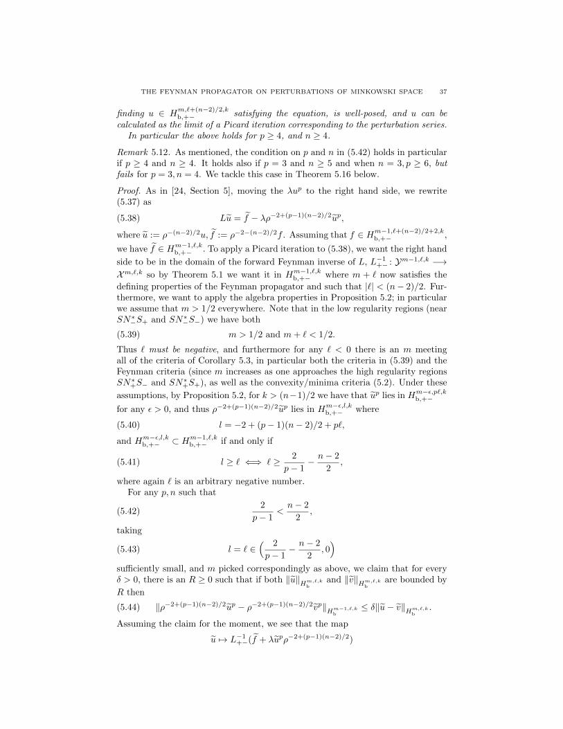
THE FEYNMAN PROPAGATOR ON PERTURBATIONS OF MINKOWSKI SPACE 37
finding u ∈ Hm,`+(n−2)/2,kb,+− satisfying the equation, is well-posed, and u can be
calculated as the limit of a Picard iteration corresponding to the perturbation series.In particular the above holds for p ≥ 4, and n ≥ 4.
Remark 5.12. As mentioned, the condition on p and n in (5.42) holds in particularif p ≥ 4 and n ≥ 4. It holds also if p = 3 and n ≥ 5 and when n = 3, p ≥ 6, butfails for p = 3, n = 4. We tackle this case in Theorem 5.16 below.
Proof. As in [24, Section 5], moving the λup to the right hand side, we rewrite(5.37) as
(5.38) Lu = f − λρ−2+(p−1)(n−2)/2up,
where u := ρ−(n−2)/2u, f := ρ−2−(n−2)/2f . Assuming that f ∈ Hm−1,`+(n−2)/2+2,kb,+− ,
we have f ∈ Hm−1,`,kb,+− . To apply a Picard iteration to (5.38), we want the right hand
side to be in the domain of the forward Feynman inverse of L, L−1+− : Ym−1,`,k −→Xm,`,k so by Theorem 5.1 we want it in Hm−1,`,k
b,+− where m + ` now satisfies the
defining properties of the Feynman propagator and such that |`| < (n− 2)/2. Fur-thermore, we want to apply the algebra properties in Proposition 5.2; in particularwe assume that m > 1/2 everywhere. Note that in the low regularity regions (nearSN∗−S+ and SN∗−S−) we have both
(5.39) m > 1/2 and m+ ` < 1/2.
Thus ` must be negative, and furthermore for any ` < 0 there is an m meetingall of the criteria of Corollary 5.3, in particular both the criteria in (5.39) and theFeynman criteria (since m increases as one approaches the high regularity regionsSN∗+S− and SN∗+S+), as well as the convexity/minima criteria (5.2). Under these
assumptions, by Proposition 5.2, for k > (n−1)/2 we have that up lies in Hm−ε,p`,kb,+−
for any ε > 0, and thus ρ−2+(p−1)(n−2)/2up lies in Hm−ε,l,kb,+− where
(5.40) l = −2 + (p− 1)(n− 2)/2 + p`,
and Hm−ε,l,kb,+− ⊂ Hm−1,`,k
b,+− if and only if
(5.41) l ≥ ` ⇐⇒ ` ≥ 2
p− 1− n− 2
2,
where again ` is an arbitrary negative number.For any p, n such that
(5.42)2
p− 1<n− 2
2,
taking
(5.43) l = ` ∈( 2
p− 1− n− 2
2, 0)
sufficiently small, and m picked correspondingly as above, we claim that for everyδ > 0, there is an R ≥ 0 such that if both ‖u‖Hm,`,kb
and ‖v‖Hm,`,kbare bounded by
R then
(5.44) ‖ρ−2+(p−1)(n−2)/2up − ρ−2+(p−1)(n−2)/2vp‖Hm−1,`,kb
≤ δ‖u− v‖Hm,`,kb.
Assuming the claim for the moment, we see that the map
u 7→ L−1+−(f + λupρ−2+(p−1)(n−2)/2)

38 JESSE GELL-REDMAN, NICK HABER, AND ANDRAS VASY
is a contraction mapping on Hm,`,kb and thus the Picard iteration un+1 = L−1+−(f +
λupnρ−2+(p−1)(n−2)/2) with u1 = 0 converges if f is sufficiently small in Hm−1,`,k
b
(as assumed in the theorem).Thus it remains only to prove the claim. For any ` and for any ε > 0 we have
‖up − vp‖Hm−ε,p`,kb=∥∥∥(u− v)
p−1∑j=0
uj vp−1−j∥∥∥Hm−ε,p`,kb
≤ C‖u− v‖Hm,`,kbmax(‖u‖Hm,`,kb
, ‖u‖Hm,`,kb)p−1
(5.45)
provided m−(p−2)µ > 1/2. Since ` satisfies (5.41) with l as in (5.43), by bounding
the Hm,`,kb norm with the Hm,l,k
b norm,
‖ρ−2+(p−1)(n−2)/2up − ρ−2+(p−1)(n−2)/2vp‖Hm−ε,`,kb≤ ‖up − vp‖Hm−ε,p`,kb
,
and combining with (5.45) gives the claim once µ > 0 is taken sufficiently small. �
To extend to p = 3, n = 4, we need improvements of the regularity properties forproducts which allow us to take the weight l to be greater than zero. To do so andstill have m+ l < 1/2 in the low regularity zone, we need m < 1/2, which is belowthe regularity threshold in the work in Section 5.5; thus we need improvementsof the results therein. The necessary improvements are based on the ideas in thefollowing.
Lemma 5.13. Let s, s′, s0 ∈ R. Let u, v ∈ Hs0 , then WFs′(uv) ⊂ WFs(v), pro-
vided s ≥ s0 ≥ s′ and s− s′ + s0 > n/2.
The point here is that one can take s0 < n/2, and obtain a result for uv whichsays it is in a worse Sobolev space then Hs0 microlocally provided v is in a betterone microlocally.
The proof in fact follows the first of the product regularity arguments above,namely that (5.11) implies (5.10). Consider a point ξ0 with (x0, ξ0) 6∈WFs(v), anda function s ≥ s0 which equals s on an open cone C ⊂ (WFs(v))comp and takes′ ≡ s0 outside some compact set K ⊂ C, s′ ≡ s′ near ξ0 with s′ ≤ s everywhere;as we show this implies that Hs · Hs0 ⊂ Hs′ . Indeed, this is analogous to (5.12)above, and we break the relevant integral Iξ up in the same way as in (5.15), so wemust bound integrals
supξ∈K
∫1
〈η〉2s−2s′〈ξ − η〉2s0dη and sup
ξ∈K
∫1
〈η〉2s〈ξ − η〉2s0−2s′dη.
The second integral is bounded by the arguments above, and for the first integral,the only difference is that over the set C, using that s− s′ ≥ 0 there, we have∫
C
1
〈η〉2s−2s′〈ξ − η〉2s0dη ≤
∫C
1
〈ξ − η〉2(s−s′+s0)dη ≤
∫C
1
〈ξ − η〉2(s−s′+s0)dη,
which is finite since s − s′ + s0 > n/2. The rest of the estimates are exactly as inthe previous case.
Applying this line of thinking to the model spaces Ym,ad defined in (5.16), we canobtain a regularity result for products which allows us to dip under the thresholdd/2 above.

THE FEYNMAN PROPAGATOR ON PERTURBATIONS OF MINKOWSKI SPACE 39
Lemma 5.14. For m,m′,m0, a ∈ R such that m−m′ +m0 > d/2, a > (n− d)/2
and m ≥ m0 ≥ m′, we have Ym0,ad · Ym,a ⊂ Ym′,a. Furthermore,
(5.46) WFm′+a(uv) ⊂ (WFm+a(u) + WFm+a(v)) ∪WFm+a(u) ∪WFm+a(v).
Proof. To see that the first conclusion holds, we argue as in Lemma 5.5, and thususe the inequality ∫ (
〈ξ〉m′〈ξ′′〉a
〈ξ − η〉m0〈ξ′′ − η′′〉a〈η〉m〈η′′〉a
)2
dη
≤2∑
i,j=1
∫ (figj
〈ξ − η〉m〈ξ′′ − η′′〉a〈η′′〉a
)2
dη,
(5.47)
where f1 = 〈η〉m′ , f2 = 〈ξ − η〉m′ and g1 = 〈η′′〉a, g2 = 〈ξ′′ − η′′〉a. Replacing theunprimed variable with primed variables and using that both∫ (
〈η′〉m′
〈ξ − η′〉m0〈η′〉m
)2
dη′,
∫ (〈ξ′ − η′〉m′
〈ξ − η′〉m0〈η′〉m
)2
dη′
are uniformly bounded under the stated assumptions on m,m′,m0 gives the state-ment.
The wavefront set containment is obtained by locating similar improvements inthe proof of Lemma 5.7. Indeed, as there, we have that u ∈ H(w1), v ∈ H(w2) wherewi(ξ) = 〈ξ〉m0〈ξ′′〉a + 〈ξ〉si where si = si(ξ) where the si ≡ m + a off open conic
sets Ci are arbitrary open sets containing, respectively, WFm+a(u) and WFm+a(v).We want to show that given
ξ 6∈ (WFm+a(u) + WFm+a(v)) ∪WFm+a(u) ∪WFm+a(v)
and a proper choice of function s with s = m′ + a near ξ that uv ∈ Hs, whichamounts to applying Lemma 5.4 with w = s and w1, w2 exactly as in Lemma 5.7.
We thus want to bound an integral similar to (5.25), namely∫ ( 〈ξ〉s
(〈η〉m0〈η′′〉k + 〈η〉s1)(〈ξ − η〉m0〈ξ′′ − η′′〉k + 〈ξ − η〉s2)
)2dη,
We choose s so that s ≤ m + a and bound 〈ξ〉2s . 〈η〉2(m+a) + 〈ξ − η〉2(m+a) andas usual break the integral into two parts involving the two terms on the right of
this bound. Again we focus on the 〈η〉2s term. Integrating first over C1 and then
(C1)comp; over Cc1, we have that 〈η〉m〈η′′〉k + 〈η〉s1 > (1/2)〈η〉s, so that part of the
integral with 〈η〉2s in the numerator over C1 is bounded by∫ ( 1
〈η〉s1−s〈ξ − η〉m〈ξ′′ − η′′〉k + 〈ξ − η〉s2)2dη
≤∫ ( 1
〈η′〉m−m′〈ξ′ − η′〉m0〈ξ′′ − η′′〉k,)2dη.
which, by separating into primed and double primed coordinates and using theassumptions on m,m0,m
′ is uniformly bounded. The rest of the bounds proceedanalogously and are left to the reader.
�

40 JESSE GELL-REDMAN, NICK HABER, AND ANDRAS VASY
By reducing locally and arguing exactly as in the proof of Proposition 5.2 andCorollary 5.3, we obtain
Proposition 5.15. For ` sufficiently small, there exists m : bS∗M −→ R satisfying:1) that m ≥ 1/2 − δ for some δ ∈ (0, 1/2), 2) m, ` satisfy the forward Feynmancondition in the strengthened form given in Theorem 3.3, and 3) m satisfies thecondition on the sublevel sets and minima in (5.2). Then for k ∈ N satisfyingk > (n− 1)/2,
Hm,l1,kb,+− Hm,l2,k
b,+− ⊂ Hm−2δ−0,l1+l2,kb,+− .
In particular, for δ sufficiently small (Hm,l1,kb,+− )3 ⊂ Hm−4δ−0,l1+l2,k
b,+− .
We can now finally prove
Theorem 5.16 (p = 3, n = 4). Suppose g is a perturbation of Minkowski spacein the sense of Lorentzian scattering metrics (see Section 2), in particular so thatTheorem 5.1 holds. In dimension n = 4, given λ ∈ R and a weight ` ≥ 0 and `sufficiently small, there is C > 0 such that the small-data Feynman problem, i.e.given
f ∈ Hm−1,`+(n−2)/2+2,kb,+− with norm < C
finding u ∈ Hm,`+(n−2)/2,kb,+− satisfying
(5.48) �g,+−u+ λu3 = f,
is well-posed, and u can again be calculated as the limit of a Picard iteration corre-sponding to the perturbation series.
Remark 5.17. Although we do not state it here explicitly, Proposition 5.15 alsogives improvements to the statement of Theorem 5.11 for other n, p in terms of thespaces in which solvability holds (what ` can be), though not for whether there isa space of the kind considered there in which solvability holds.
Proof. The proof is identical to that of Theorem 5.11 incorporating the improve-ments given by Proposition 5.15. We take ` ≥ 0 and find an m such that m + `satisfies the Feynman condition and m > 1/2− δ for some small δ > 0. Rewriting
the equation as in (5.38) with f and u defined in the same way, and assuming that
f ∈ Hm,`,kb,+− , the condition that
ρ2−(p−1)(n−2)/2up = ρ4−nu3 ∈ Hm−5δ,`,kb,+− ⊂ Hm−1,`,k
b,+−
is now that δ be less than 1/5 and that
(5.49) ` ≤ 4− n+ 3` ⇐⇒ ` ≥ n/2− 2.
If n = 4, we can thus find ` and m satisfying the Feynman conditions and (5.49)simultaneously. From now on we assume that n = 4. The existence of an msatisfying the conditions in (5.2) is a trivial modification of the proof of Corollary5.3.
The Picard iteration argument is now identical to that in Theorem 5.11 exceptincorporating the loss in Proposition 5.15. In this case, the claim in 5.44 is substi-tuted by the following: for every δ > 0 sufficiently small, there is an R ≥ 0 suchthat if both ‖u‖Hm−δ,`,kb
and ‖v‖Hm−δ,`,kbare bounded by R then
‖u3 − v3‖Hm−5δ,`,kb
≤ δ‖u− v‖Hm−δ,`,kb.

THE FEYNMAN PROPAGATOR ON PERTURBATIONS OF MINKOWSKI SPACE 41
This and the rest of the proof follow exactly as in Theorem 5.11 using the improve-ment in Proposition 5.14. �
References
[1] D. Baskin, A. Vasy, and J. Wunsch. Asymptotics of scalar waves on long-range asymptotically
minkowski spaces. Manucript, In preparation.
[2] Dean Baskin, Andras Vasy, and Jared Wunsch. Asymptotics of radiation fields in asymptot-ically Minkowski space. arXiv:1212.5141, 2012.
[3] Lydia Bieri. Part I: Solutions of the Einstein vacuum equations. In Extensions of the stability
theorem of the Minkowski space in general relativity, volume 45 of AMS/IP Stud. Adv. Math.,pages 1–295. Amer. Math. Soc., Providence, RI, 2009.
[4] Lydia Bieri and Nina Zipser. Extensions of the stability theorem of the Minkowski space
in general relativity, volume 45 of AMS/IP Studies in Advanced Mathematics. AmericanMathematical Society, Providence, RI, 2009.
[5] R. Brunetti, K. Fredenhagen, and M. Kohler. The microlocal spectrum condition and Wickpolynomials of free fields on curved spacetimes. Comm. Math. Phys., 180(3):633–652, 1996.
[6] Romeo Brunetti and Klaus Fredenhagen. Microlocal analysis and interacting quantum field
theories: renormalization on physical backgrounds. Comm. Math. Phys., 208(3):623–661,2000.
[7] Gilles Carron, Thierry Coulhon, and Andrew Hassell. Riesz transform and Lp-cohomology
for manifolds with Euclidean ends. Duke Math. J., 133(1):59–93, 2006.[8] Demetrios Christodoulou. Global solutions of nonlinear hyperbolic equations for small initial
data. Comm. Pure Appl. Math., 39(2):267–282, 1986.
[9] Demetrios Christodoulou and Sergiu Klainerman. The global nonlinear stability of theMinkowski space, volume 41 of Princeton Mathematical Series. Princeton University Press,
Princeton, NJ, 1993.
[10] Piotr T. Chrusciel and Szymon Leski. Polyhomogeneous solutions of nonlinear wave equationswithout corner conditions. J. Hyperbolic Differ. Equ., 3(1):81–141, 2006.
[11] Claudio Dappiaggi, Valter Moretti, and Nicola Pinamonti. Rigorous steps towards holographyin asymptotically flat spacetimes. Rev. Math. Phys., 18(4):349–415, 2006.
[12] Claudio Dappiaggi, Valter Moretti, and Nicola Pinamonti. Cosmological horizons and recon-
struction of quantum field theories. Comm. Math. Phys., 285(3):1129–1163, 2009.[13] Kiril Datchev and Andras Vasy. Gluing semiclassical resolvent estimates via propagation of
singularities. Int. Math. Res. Not. IMRN, (23):5409–5443, 2012.
[14] J. J. Duistermaat and L. Hormander. Fourier integral operators. II. Acta Math., 128(3-4):183–269, 1972.
[15] F. Finster and A. Strohmaier. Gupta-Bleuer quantization of the Maxwell field in globally
hyperbolic spacetimes. Preprint, arXiv:1307.1632, 2014.[16] C. Gerard and M. Wrochna. Construction of Hadamard states by pseudo-differential calculus.
Comm. Math. Phys., 325(2):713–755, 2014.
[17] C. Gerard and M. Wrochna. Hadamard states for the linearized Yang-Mills equation oncurved spacetime. Preprint, arxiv:1403.7153, 2014.
[18] Robert Geroch. Domain of dependence. J. Mathematical Phys., 11:437–449, 1970.[19] Colin Guillarmou and Andrew Hassell. Resolvent at low energy and Riesz transform for
Schrodinger operators on asymptotically conic manifolds. I. Math. Ann., 341(4):859–896,
2008.[20] Nick Haber and Andras Vasy. Propagation of singularities around a Lagrangian submanifold
of radial points. arXiv:1110.1419, 2011.[21] P. Hintz. Global well-posedness of quasilinear wave equations on asymptotically de sitter
spaces. Preprint, arXiv:1311.6859, 2013.[22] P. Hintz and A. Vasy. Non-trapping estimates near normally hyperbolic trapping. Preprint,
arXiv:1306.4705, 2013.[23] Peter Hintz and Andras Vasy. Global analysis of quasilinear wave equations on asymptotically
Kerr-de Sitter spaces. arXiv:1306.4705, 2013.
[24] Peter Hintz and Andras Vasy. Semilinear wave equations on asymptotically de Sitter, Kerr-deSitter, and Minkowski spacetimes. arXiv:1306.4705, 2013.

42 JESSE GELL-REDMAN, NICK HABER, AND ANDRAS VASY
[25] P. D. Hislop and I. M. Sigal. Introduction to spectral theory, volume 113 of Applied Mathemat-
ical Sciences. Springer-Verlag, New York, 1996. With applications to Schrodinger operators.
[26] Lars Hormander. On the existence and the regularity of solutions of linear pseudo-differentialequations. Enseignement Math. (2), 17:99–163, 1971.
[27] Lars Hormander. Lectures on nonlinear hyperbolic differential equations, volume 26 of
Mathematiques & Applications (Berlin) [Mathematics & Applications]. Springer-Verlag,Berlin, 1997.
[28] S. Klainerman. The null condition and global existence to nonlinear wave equations. In Non-
linear systems of partial differential equations in applied mathematics, Part 1 (Santa Fe,N.M., 1984), volume 23 of Lectures in Appl. Math., pages 293–326. Amer. Math. Soc., Prov-
idence, RI, 1986.
[29] Sergiu Klainerman. Uniform decay estimates and the Lorentz invariance of the classical waveequation. Comm. Pure Appl. Math., 38(3):321–332, 1985.
[30] Hans Lindblad. Global solutions of quasilinear wave equations. Amer. J. Math., 130(1):115–157, 2008.
[31] Hans Lindblad and Igor Rodnianski. Global existence for the Einstein vacuum equations in
wave coordinates. Comm. Math. Phys., 256(1):43–110, 2005.[32] Hans Lindblad and Igor Rodnianski. The global stability of Minkowski space-time in harmonic
gauge. Ann. of Math. (2), 171(3):1401–1477, 2010.
[33] Rafe Mazzeo and Andras Vasy. Analytic continuation of the resolvent of the Laplacian onSL(3)/SO(3). Amer. J. Math., 126(4):821–844, 2004.
[34] Rafe Mazzeo and Andras Vasy. Analytic continuation of the resolvent of the Laplacian on
symmetric spaces of noncompact type. J. Funct. Anal., 228(2):311–368, 2005.[35] Richard B. Melrose. The Atiyah-Patodi-Singer index theorem, volume 4 of Research Notes
in Mathematics. A K Peters Ltd., Wellesley, MA, 1993.
[36] Richard B. Melrose. Spectral and scattering theory for the Laplacian on asymptotically Eu-clidian spaces. In Spectral and scattering theory (Sanda, 1992), volume 161 of Lecture Notes
in Pure and Appl. Math., pages 85–130. Dekker, New York, 1994.[37] Jason Metcalfe and Daniel Tataru. Global parametrices and dispersive estimates for variable
coefficient wave equations. Math. Ann., 353(4):1183–1237, 2012.
[38] Valter Moretti. Quantum out-states holographically induced by asymptotic flatness: invari-ance under spacetime symmetries, energy positivity and Hadamard property. Comm. Math.
Phys., 279(1):31–75, 2008.
[39] Stephane Nonnenmacher and Maciej Zworski. Quantum decay rates in chaotic scattering.Acta Math., 203(2):149–233, 2009.
[40] Marek J. Radzikowski. Micro-local approach to the Hadamard condition in quantum field
theory on curved space-time. Comm. Math. Phys., 179(3):529–553, 1996.[41] Michael E. Taylor. Partial differential equations I. Basic theory, volume 115 of Applied Math-
ematical Sciences. Springer, New York, second edition, 2011.
[42] Michael E. Taylor. Partial differential equations II. Qualitative studies of linear equations,volume 116 of Applied Mathematical Sciences. Springer, New York, second edition, 2011.
[43] Andras Vasy. Microlocal analysis of asymptotically hyperbolic and Kerr-de Sitter spaces (withan appendix by Semyon Dyatlov). Invent. Math., 194(2):381–513, 2013.
[44] Andras Vasy. Microlocal analysis of asymptotically hyperbolic spaces and high-energy resol-
vent estimates. In Inverse problems and applications: inside out. II, volume 60 of Math. Sci.Res. Inst. Publ., pages 487–528. Cambridge Univ. Press, Cambridge, 2013.
[45] N. D. Viet. Renormalization of quantum field theory on curved space-times, a causal approach.Preprint, arxiv:1312.5674, 2013.
[46] F. Wang. Radiation field for vacuum Einstein equation. PhD thesis, Massachusetts Institute
of Technology, 2010. arXiv:1304.0407.
Department of Mathematics, Johns Hopkins University, MD 21218
E-mail address: [email protected]
MSRI, Berkeley and McGill University, Montreal.
E-mail address: [email protected]
Department of Mathematics, Stanford University, CA 94305-2125, USAE-mail address: [email protected]


![arXiv:1310.7888v1 [math.AP] 29 Oct 2013Zelditch).pdf · and Fourier Tauberian theorems. The wave equation techniques mainly involve the construc-tion of parametrices for the fundamental](https://img.pdfslide.us/doc/110x75/60f836e9119914661133d687/arxiv13107888v1-mathap-29-oct-2013-zelditchpdf-and-fourier-tauberian-theorems.jpg)
![arXiv:1611.09296v1 [cs.DS] 28 Nov 2016stefan/netup-dag-arxiv.pdf · arXiv:1611.09296v1 [cs.DS] 28 Nov 2016 Congestion-Free Rerouting of Flows on DAGs⋆ Saeed Akhoondian Amiri1 Szymon](https://img.pdfslide.us/doc/110x75/60383aa6d02f533dca5e1917/arxiv161109296v1-csds-28-nov-2016-stefannetup-dag-arxivpdf-arxiv161109296v1.jpg)

![arXiv:1202.5249v1 [cs.RO] 23 Feb 2012acg.cs.tau.ac.il/projects/mms/papers/arxiv.pdf · abilistic completeness proof for the most prevalent case, namely MMS with samples that are a](https://img.pdfslide.us/doc/110x75/5b8587f57f8b9a784a8e87cf/arxiv12025249v1-csro-23-feb-abilistic-completeness-proof-for-the-most-prevalent.jpg)

![arXiv:1410.0440v1 [cs.LG] 2 Oct 2014djhsu/papers/apple-arxiv.pdf · Scalable Nonlinear Learning with Adaptive Polynomial Expansions Alekh Agarwal 1, Alina Beygelzimer2, Daniel Hsu3,](https://img.pdfslide.us/doc/110x75/6054bc74a7739e523e34e65e/arxiv14100440v1-cslg-2-oct-djhsupapersapple-arxivpdf-scalable-nonlinear.jpg)
![arXiv:submit/2340273 [cs.CV] 24 Jul 2018cocosci.princeton.edu/papers/deep-sim-arxiv.pdf · understanding (LeCun, Bengio, & Hinton, 2015), among other breakthroughs in natural language](https://img.pdfslide.us/doc/110x75/601f3dd5aa680b4e06665cf7/arxivsubmit2340273-cscv-24-jul-understanding-lecun-bengio-hinton.jpg)