Embed Size (px)
Citation preview
11-755/18-797 Machine Learning for Signal Processing
IntroductionSignal representation
Class 1. 24 August 2010
Instructor: Bhiksha Raj
24 Aug 2010 11-755/18-797 1
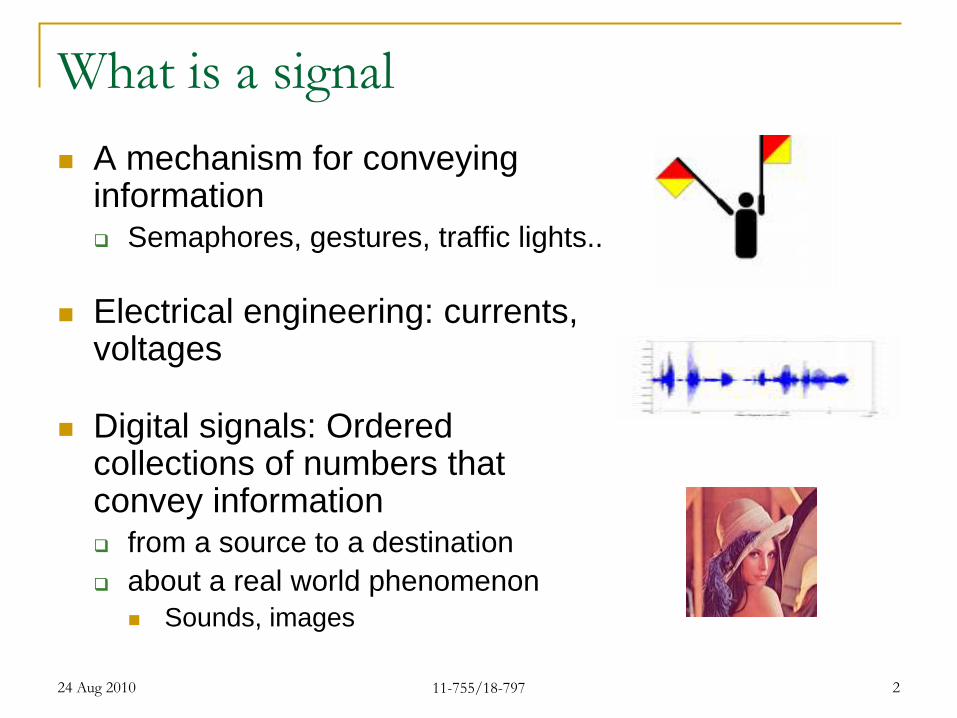
What is a signal A mechanism for conveying
information Semaphores, gestures, traffic lights..
Electrical engineering: currents, voltages
Digital signals: Ordered collections of numbers that convey information from a source to a destination about a real world phenomenon
Sounds, images
24 Aug 2010 11-755/18-797 2

Signal Examples: Audio
A sequence of numbers [n1 n2 n3 n4 …] The order in which the numbers occur is important
Ordered Represent a perceivable sound
24 Aug 2010 11-755/18-797 3
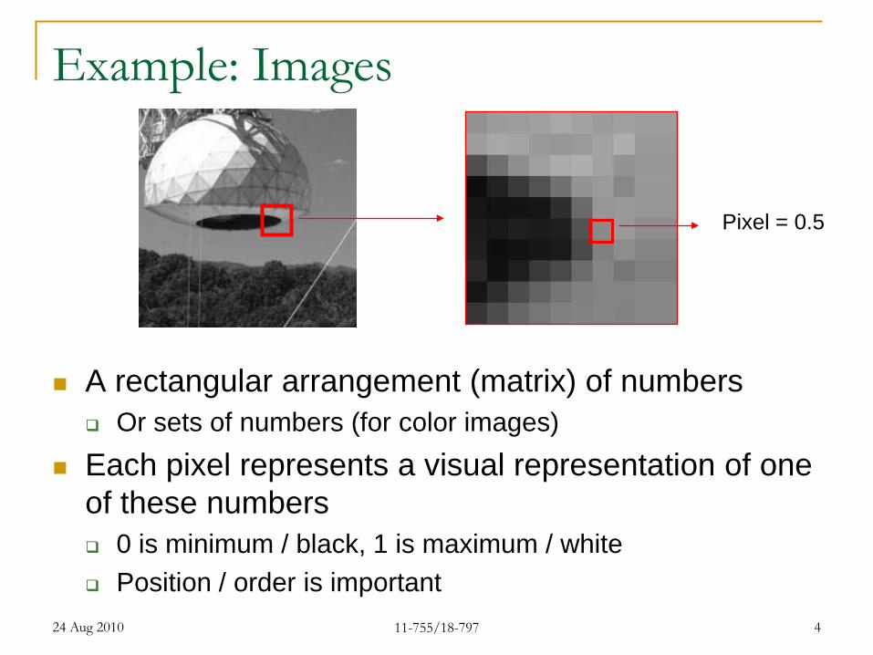
Example: Images
A rectangular arrangement (matrix) of numbers Or sets of numbers (for color images)
Each pixel represents a visual representation of one of these numbers 0 is minimum / black, 1 is maximum / white Position / order is important
Pixel = 0.5
24 Aug 2010 11-755/18-797 4

What is Signal Processing
Analysis, Interpretation, and Manipulation of signals. Decomposition: Fourier transforms, wavelet
transforms Denoising signals Coding: GSM, LPC, Mpeg, Ogg Vorbis Detection: Radars, Sonars Pattern matching: Biometrics, Iris recognition,
finger print recognition Etc.
24 Aug 2010 11-755/18-797 5

What is Machine Learning The science that deals with the development of
algorithms that can learn from data Learning patterns in data
Automatic categorization of text into categories; Market basket analysis
Learning to classify between different kinds of data Spam filtering: Valid email or junk?
Learning to predict data Weather prediction, movie recommendation
Statistical analysis and pattern recognition when performed by a computer scientist..
24 Aug 2010 11-755/18-797 6

MLSP The application of Machine Learning techniques to the analysis of
signals such as audio, images and video Learning to characterize signals in a data driven manner
What are they composed of? Can we automatically deduce that the fifth symphony is composed of notes? Can we segment out components of images? Can we learn the sparsest way to represent any signal
Learning to detect signals Radars. Face detection. Speaker verification
Learning to recognize themes in signals Face recognition. Speech recognition.
Learning to: interpret; optimally represent etc
In some sense, a combination of signal processing and machine learning But also includes learning based methods (as opposed to deterministic
methods) for data analysis
24 Aug 2010 11-755/18-797 7

MLSP IEEE Signal Processing Society has an MLSP committee:
The Machine Learning for Signal Processing Techinical Committee (MLSP TC) is at the interface between theory and application, developing novel theoretically-inspired methodologies targeting both longstanding and emergent signal processing applications. Central to MLSP is on-line/adaptive nonlinear signal processing and data-driven learning methodologies. Since application domains provide unique problem constraints/assumptions and thus motivate and drive signal processing advances, it is only natural that MLSP research has a broad application base. MLSP thus encompasses new theoretical frameworks for statistical signal processing (e.g. machine learning-based and information-theoretic signal processing), new and emerging paradigms in statistical signal processing (e.g. independent component analysis (ICA), kernel-based methods, cognitive signal processing) and novel developments in these areas specialized to the processing of a variety of signals, including audio, speech, image, multispectral, industrial, biomedical, and genomic signals.
24 Aug 2010 11-755/18-797 8

MLSP: Fast growing field IEEE Workshop on Machine Learning for Signal Processing
Held this year in Finland. Aug 29-Sep 1, http/mlsp2010.conwiz.dk/ MLSP 2011 is to be held in Beijing, China
Used everywhere Biometrics: Face recognition, speaker identification User interfaces: Gesture based UIs, voice-based retrieval voice
UIs, music retrieval Data capture: Optical character recognition. Compressive sensing Network traffic analysis: Routing algorithms for bits and vehicular
traffic
Synergy with other topics (text / genome)
24 Aug 2010 11-755/18-797 9

In this Course Jetting through fundamentals:
Signal Processing, Linear Algebra, Probability
Sounds: Characterizing sounds Denoising speech Synthesizing speech Separating sounds in mixtures Processing music.
Images: Characterization Denoising Object detection and recognition Face recognition Biometrics
Representation: Transform methods Compressive sensing.
Topics covered are representative Actual list to be covered may change, depending on how the course progresses
24 Aug 2010 11-755/18-797 10

Required Background DSP
Fourier transforms, linear systems, basic statistical signal processing
Linear Algebra Definitions, vectors, matrices, operations, properties
Probability Basics: what is an random variable, probability
distributions, functions of a random variable
Machine learning Learning, modelling and classification techniques
24 Aug 2010 11-755/18-797 11

Guest Lectures Several guest lectures by experts in the topics
Alan Black (CMU) Statistical speech synthesis Voice morphing
Fernando de la Torre (CMU) Data representations
Marios Savvides Iris recognition
Vijay Kumar Super resolution for face recognition
Petros Boufounos (Mitsubishi) Compressive Sensing
24 Aug 2010 11-755/18-797 12

Guest Lectures Several guest lectures by experts in the topics
Rahul Sukhtankar (Intel) Face detection
Mario Berges Load monitoring
John McDonough Microphone arrays
Subject to change Guest lecturers are notorious for having schedule changes If the guest lecturer is unavailable, the topic will be covered by me
24 Aug 2010 11-755/18-797 13
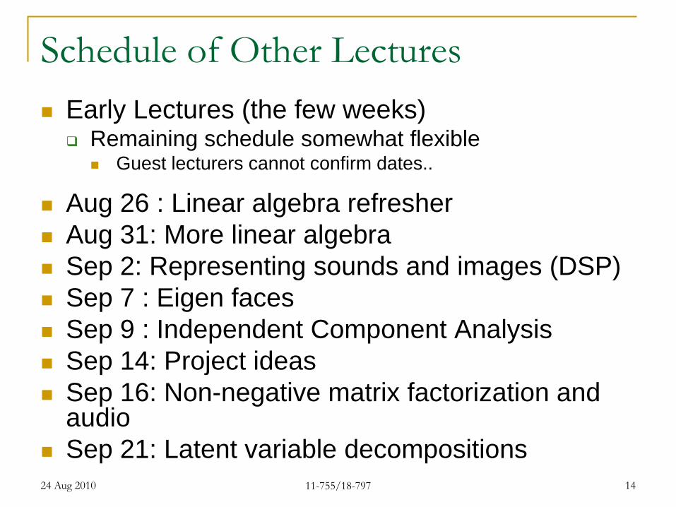
Schedule of Other Lectures Early Lectures (the few weeks)
Remaining schedule somewhat flexible Guest lecturers cannot confirm dates..
Aug 26 : Linear algebra refresher Aug 31: More linear algebra Sep 2: Representing sounds and images (DSP) Sep 7 : Eigen faces Sep 9 : Independent Component Analysis Sep 14: Project ideas Sep 16: Non-negative matrix factorization and
audio Sep 21: Latent variable decompositions24 Aug 2010 11-755/18-797 14

Grading
Homework assignments : 50% Mini projects Will be assigned during course 3 in all
Final project: 50% Will be assigned early in course No classes on Nov. 25 or Nov 30 to give you time
for the project Dec 2: Poster presentation for all projects, with
demos (if possible) Partially graded by visitors to the poster
24 Aug 2010 11-755/18-797 15

Projects: 2009 Statistical Klatt Parametric Synthesis Augmented Reality / Seam Carving / Audio Content-aware resizing for video Voice transformation with Canonical Correlation Analysis Talking Karaoke Sound source separation and missing feature
enhancement Voice transformation Image segmentation Non-intrusive load monitoring Counting blood cells in Cerebrospinal fluid Determining Music tablature Image Deblurring
24 Aug 2010 11-755/18-797 16

Instructor and TA Instructor: Prof. Bhiksha Raj
Room 6705 Hillman Building [email protected] 412 268 9826
TA: Sourish Chaudhuri
Office Hours: Bhiksha Raj: Mon 3:00-4.00 TA: TBD Available by email: [email protected]
Hillman
Windows
My office
Forbes
24 Aug 2010 11-755/18-797 17

Additional Administrivia
Website: http://mlsp.cs.cmu.edu/courses/fall2010/ Lecture material will be posted on the day of each
class on the website Reading material and pointers to additional
information will be on the website
Discussion board blackboard.andrew.cmu.edu/
24 Aug 2010 11-755/18-797 18
Representing Data
Audio
Images Video
Other types of signals In a manner similar to one of the above
24 Aug 2010 11-755/18-797 19

What is an audio signal A typical audio signal It’s a sequence of points
24 Aug 2010 11-755/18-797 20

Where do these numbers come from?
Any sound is a pressure wave: alternating highs and lows of air pressure moving through the air
When we speak, we produce these pressure waves Essentially by producing puff after puff of air Any sound producing mechanism actually produces pressure waves
These pressure waves move the eardrum Highs push it in, lows suck it out We sense these motions of our eardrum as “sound”
Pressure highs
Spaces betweenarcs show pressurelows
24 Aug 2010 11-755/18-797 21

SOUND PERCEPTION
24 Aug 2010 11-755/18-797 22

Storing pressure waves on a computer The pressure wave moves a diaphragm
On the microphone The motion of the diaphragm is converted to
continuous variations of an electrical signal Many ways to do this
A “sampler” samples the continuous signal at regular intervals of time and stores the numbers
24 Aug 2010 11-755/18-797 23
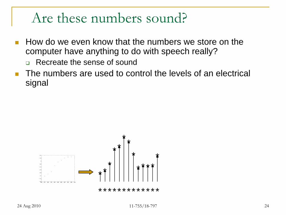
Are these numbers sound? How do we even know that the numbers we store on the
computer have anything to do with speech really? Recreate the sense of sound
The numbers are used to control the levels of an electrical signal
The electrical signal moves a diaphragm back and forth to produce a pressure wave That we sense as sound
************
****
****
****
*
*
24 Aug 2010 11-755/18-797 24
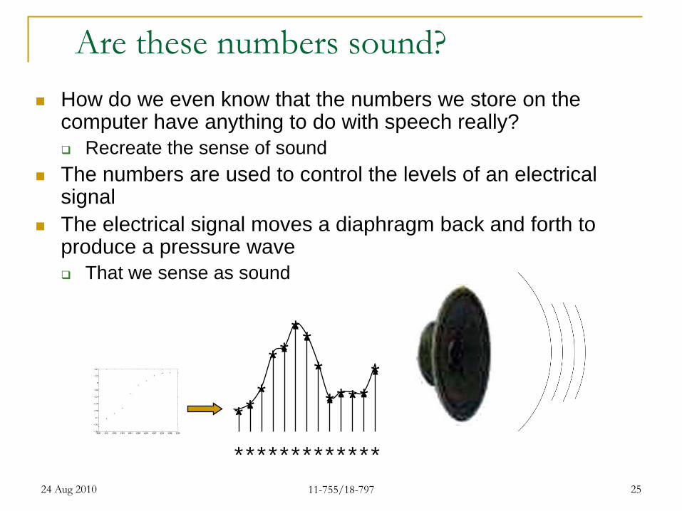
Are these numbers sound? How do we even know that the numbers we store on the
computer have anything to do with speech really? Recreate the sense of sound
The numbers are used to control the levels of an electrical signal
The electrical signal moves a diaphragm back and forth to produce a pressure wave That we sense as sound
************
****
****
****
*
*
24 Aug 2010 11-755/18-797 25

How many samples a second Convenient to think of sound in terms of
sinusoids with frequency
Sounds may be modelled as the sum of many sinusoids of different frequencies Frequency is a physically motivated unit Each hair cell in our inner ear is tuned to
specific frequency
Any sound has many frequency components We can hear frequencies up to 16000Hz
Frequency components above 16000Hz can be heard by children and some young adults
Nearly nobody can hear over 20000Hz.
0 10 20 30 40 50 60 70 80 90 100-1
-0.5
0
0.5
1
←P
ress
ure→
A sinusoid
24 Aug 2010 11-755/18-797 26

Signal representation - Sampling Sampling frequency (or sampling rate) refers
to the number of samples taken a second
Sampling is measured in Hz We need a sample rate twice as high as the
highest frequency we want to represent (Nyquist freq)
For our ears this means a sample rate of at least 40kHz Cause we hear up to 20kHz
Common sample rates For speech 8kHz to 16kHz For music 32kHz to 44.1kHz Pro-equipment 96kHz When in doubt use 44.1kHz
****
****
*****
Time in secs.
24 Aug 2010 11-755/18-797 27

Aliasing Low sample rates result in aliasing High frequencies are misrepresented Frequency f1 will become (sample rate – f1 ) In video also when you see wheels go
backwards
24 Aug 2010 11-755/18-797 28

Aliasing examples
Time
Freq
uenc
y
0 0.1 0.2 0.3 0.4 0.5 0.6 0.7 0.8 0.90
0.5
1
1.5
2
x 104
Time
Freq
uenc
y
0 0.1 0.2 0.3 0.4 0.5 0.6 0.7 0.8 0.90
2000
4000
6000
8000
10000
Time
Freq
uenc
y
0 0.1 0.2 0.3 0.4 0.5 0.6 0.7 0.8 0.90
1000
2000
3000
4000
5000
Sinusoid sweeping from 0Hz to 20kHz44kHz SR, is ok 22kHz SR, aliasing! 11kHz SR, double aliasing!
On real sounds
at 44kHz
at 22kHz
at 11kHz
at 5kHz
at 4kHz
at 3kHz
On videoOn images
24 Aug 2010 11-755/18-797 29

Avoiding Aliasing
Sound naturally has all perceivable frequencies And then some Cannot control the rate of variation of pressure waves in
nature Sampling at any rate will result in aliasing Solution: Filter the electrical signal before sampling
it Cut off all frequencies above samplingfrequency/2 E.g., to sample at 44.1Khz, filter the signal to eliminate all
frequencies above 22050 Hz
AntialiasingFilter Sampling
Analog signal Digital signal
24 Aug 2010 11-755/18-797 30
Storing numbers on the Computer Sound is the outcome of a continuous range of
variations The pressure wave can take any value (within limit) The diaphragm can also move continuously The electrical signal from the diaphragm has continuous
variations
A computer has finite resolution Numbers can only be stored to finite resolution E.g. a 16-bit number can store only 65536 values, while a 4-
bit number can store only 16 values To store the sound wave on the computer, the continuous
variation must be “mapped” on to the discrete set of numbers we can store
24 Aug 2010 11-755/18-797 31

Mapping signals into bits Example of 1-bit sampling table
Signal Value Bit sequence Mapped to
S > 2.5v 1 1 * const
S <=2.5v 0 0
Original Signal Quantized approximation
24 Aug 2010 11-755/18-797 32

Mapping signals into bits Example of 2-bit sampling table
Signal Value Bit sequence Mapped toS >= 3.75v 11 3 * const3.75v > S >= 2.5v 10 2 * const2.5v > S >= 1.25v 01 1 * const1.25v > S >= 0v 0 0
Original Signal Quantized approximation
24 Aug 2010 11-755/18-797 33
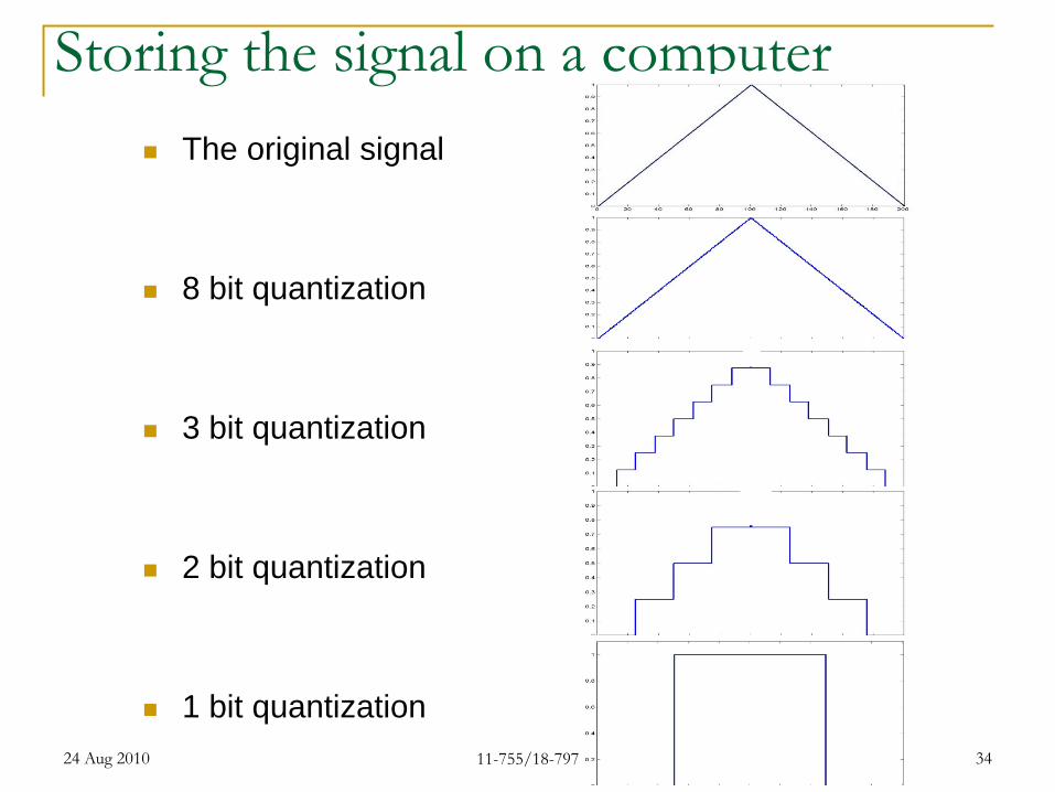
Storing the signal on a computer The original signal
8 bit quantization
3 bit quantization
2 bit quantization
1 bit quantization24 Aug 2010 11-755/18-797 34

Tom Sullivan Says his Name 16 bit sampling
5 bit sampling
4 bit sampling
3 bit sampling
1 bit sampling
24 Aug 2010 11-755/18-797 35

A Schubert Piece 16 bit sampling
5 bit sampling
4 bit sampling
3 bit sampling
1 bit sampling24 Aug 2010 11-755/18-797 36

Sampling Formats Sampling can be uniform Sample values equally spaced out
Or nonuniform
Signal Value Bits Mapped toS >= 3.75v 11 3 * const3.75v > S >= 2.5v 10 2 * const2.5v > S >= 1.25v 01 1 * const1.25v > S >= 0v 0 0
Signal Value Bits Mapped toS >= 4v 11 4.5 * const4v > S >= 2.5v 10 3.25 * const2.5v > S >= 1v 01 1.25 * const1.0v > S >= 0v 0 0.5 * const
24 Aug 2010 11-755/18-797 37

Uniform Sampling
UPON BEING SAMPLED AT ONLY 3 BITS (8 LEVELS)
24 Aug 2010 11-755/18-797 38

Uniform Sampling
At the sampling instant, the actual value of the waveform is rounded off to the nearest level permitted by the quantization
Values entirely outside the range are quantized to either the highest or lowest values
24 Aug 2010 11-755/18-797 39

Uniform Sampling
There is a lot more action in the central region than outside. Assigning only four levels to the busy central region and
four entire levels to the sparse outer region is inefficient Assigning more levels to the central region and less to the
outer region can give better fidelity for the same storage
24 Aug 2010 11-755/18-797 40

Non-uniform Sampling
Assigning more levels to the central region and less to the outer region can give better fidelity for the same storage
24 Aug 2010 11-755/18-797 41
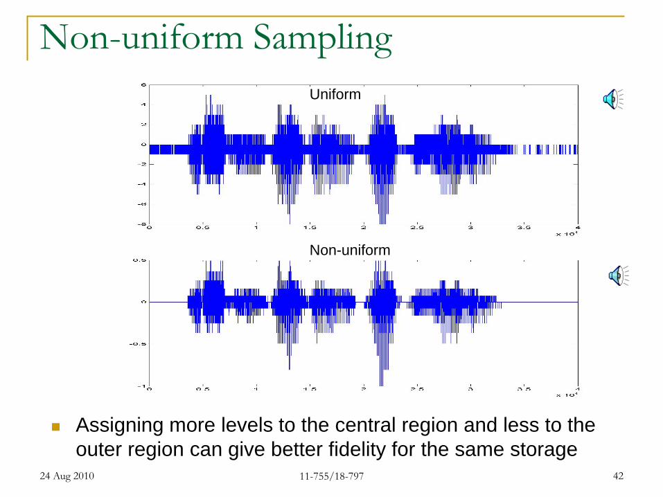
Non-uniform Sampling
Assigning more levels to the central region and less to the outer region can give better fidelity for the same storage
Uniform
Non-uniform
24 Aug 2010 11-755/18-797 42

Non-uniform Sampling
At the sampling instant, the actual value of the waveform is rounded off to the nearest level permitted by the quantization
Values entirely outside the range are quantized to either the highest or lowest values
Original Uniform Nonuniform
24 Aug 2010 11-755/18-797 43
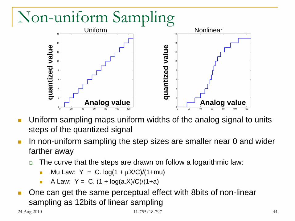
Non-uniform Sampling
Uniform sampling maps uniform widths of the analog signal to units steps of the quantized signal
In non-uniform sampling the step sizes are smaller near 0 and wider farther away The curve that the steps are drawn on follow a logarithmic law:
Mu Law: Y = C. log(1 + µX/C)/(1+mu) A Law: Y = C. (1 + log(a.X)/C)/(1+a)
One can get the same perceptual effect with 8bits of non-linear sampling as 12bits of linear sampling
NonlinearUniform
Analog valuequan
tized
val
ue
Analog valuequan
tized
val
ue
24 Aug 2010 11-755/18-797 44
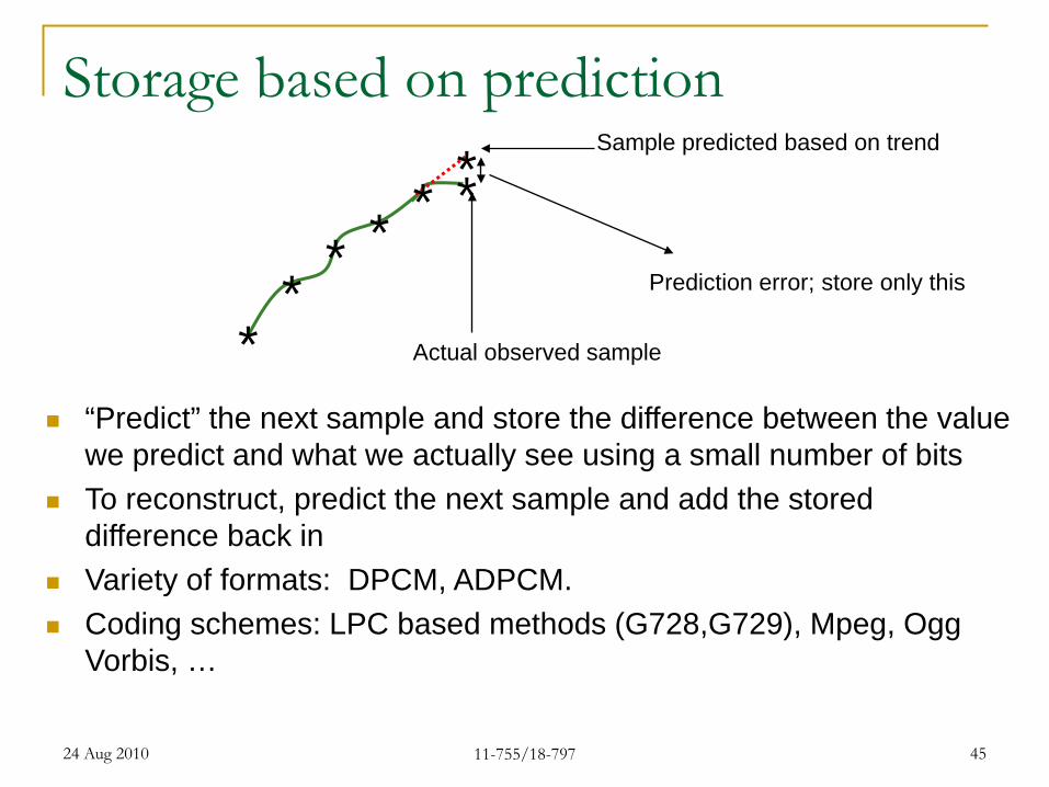
Storage based on prediction
“Predict” the next sample and store the difference between the value we predict and what we actually see using a small number of bits
To reconstruct, predict the next sample and add the stored difference back in
Variety of formats: DPCM, ADPCM. Coding schemes: LPC based methods (G728,G729), Mpeg, Ogg
Vorbis, …
**
* * * **
Actual observed sample
Sample predicted based on trend
Prediction error; store only this
24 Aug 2010 11-755/18-797 45

Dealing with audio
Capture / read audio in the format provided by the file or hardware Linear PCM, Mu-law, A-law, Coded
Convert to 16-bit PCM value I.e. map the bits onto the number on the right column This mapping is typically provided by a table computed from the sample
compression function No lookup for data stored in PCM
Conversion from Mu law: http://www.speech.cs.cmu.edu/comp.speech/Section2/Q2.7.html
Signal Value Bits Mapped toS >= 3.75v 11 33.75v > S >= 2.5v 10 22.5v > S >= 1.25v 01 11.25v > S >= 0v 0 0
Signal Value Bits Mapped toS >= 4v 11 4.54v > S >= 2.5v 10 3.252.5v > S >= 1v 01 1.251.0v > S >= 0v 0 0.5
24 Aug 2010 11-755/18-797 46

Common Audio Capture Errors Gain/Clipping: High gain
levels in A/D can result in distortion of the audio
Antialiasing: If the audio is sampled at N kHz, it must first be low-pass filtered at < N/2 kHz Otherwise high-frequency
components will alias into lower frequencies and distort them
24 Aug 2010 11-755/18-797 47
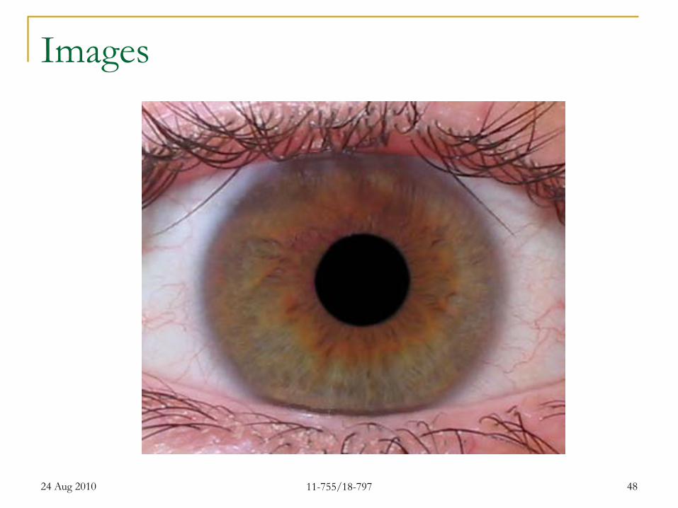
Images
24 Aug 2010 11-755/18-797 48

Images
24 Aug 2010 11-755/18-797 49

The Eye
Basic Neuroscience: Anatomy and Physiology Arthur C. Guyton, M.D. 1987 W.B.Saunders Co.
Retina
24 Aug 2010 11-755/18-797 50
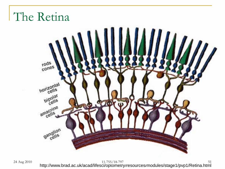
The Retina
http://www.brad.ac.uk/acad/lifesci/optometry/resources/modules/stage1/pvp1/Retina.html24 Aug 2010 11-755/18-797 51

Rods and Cones Separate Systems Rods
Fast Sensitive predominate in the
periphery Cones
Slow Not so sensitive Fovea / Macula COLOR!
Basic Neuroscience: Anatomy and Physiology Arthur C. Guyton, M.D. 1987 W.B.Saunders Co.24 Aug 2010 11-755/18-797 52

The Eye
The density of cones is highest at the fovea The region immediately surrounding the fovea is the macula
The most important part of your eye: damage == blindness Peripheral vision is almost entirely black and white
Eagles are bifoveate Dogs and cats have no fovea, instead they have an elongated slit24 Aug 2010 11-755/18-797 53

Spatial Arrangement of the Retina
(From Foundations of Vision, by Brian Wandell, Sinauer Assoc.)24 Aug 2010 11-755/18-797 54

Three Types of Cones (trichromatic vision)
Wavelength in nm
Nor
mal
ized
repo
nse
24 Aug 2010 11-755/18-797 55

Trichromatic Vision
So-called “blue” light sensors respond to an entire range of frequencies Including in the so-called “green” and “red”
regions The difference in response of “green” and
“red” sensors is small Varies from person to person
Each person really sees the world in a different color If the two curves get too close, we have color
blindness Ideally traffic lights should be red and blue
24 Aug 2010 11-755/18-797 56

White Light
24 Aug 2010 11-755/18-797 57

Response to White Light
?
24 Aug 2010 11-755/18-797 58

Response to White Light
24 Aug 2010 11-755/18-797 59
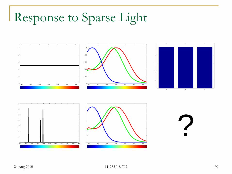
Response to Sparse Light
?24 Aug 2010 11-755/18-797 60

Response to Sparse Light
24 Aug 2010 11-755/18-797 61

The same intensity of monochromatic light will result in different perceived brightness at different wavelengths
Many combinations of wavelengths can produce the same sensation of colour.
Yet humans can distinguish 10 million colours
Human perception anomalies
Dim Bright
24 Aug 2010 11-755/18-797 62
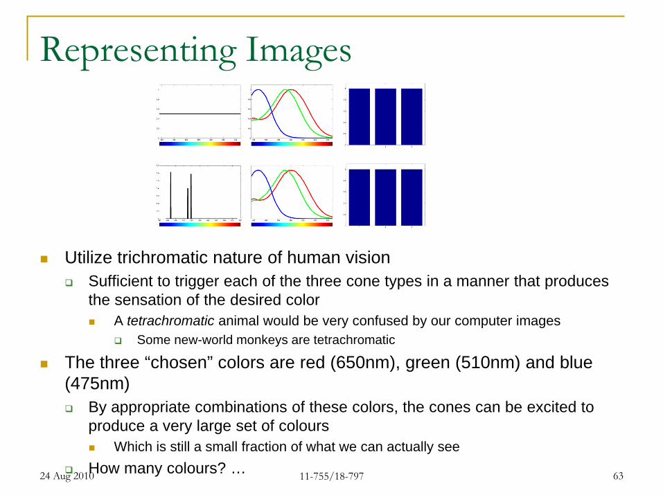
Representing Images
Utilize trichromatic nature of human vision Sufficient to trigger each of the three cone types in a manner that produces
the sensation of the desired color A tetrachromatic animal would be very confused by our computer images
Some new-world monkeys are tetrachromatic
The three “chosen” colors are red (650nm), green (510nm) and blue (475nm) By appropriate combinations of these colors, the cones can be excited to
produce a very large set of colours Which is still a small fraction of what we can actually see
How many colours? …24 Aug 2010 11-755/18-797 63

The “CIE” colour space From experiments done in the 1920s by W.
David Wright and John Guild Subjects adjusted x,y,and z on the right of a
circular screen to match a colour on the left
X, Y and Z are normalized responses of the three sensors X + Y + Z is 1.0
Normalized to have to total net intensity
The image represents all colours a person can see The outer curved locus represents monochromatic
light X,Y and Z as a function of λ
The lower line is the line of purples End of visual spectrum
The CIE chart was updated in 1960 and 1976 The newer charts are less popular
International council on illumination, 1931
24 Aug 2010 11-755/18-797 64

What is displayed The RGB triangle
Colours outside this area cannot be matched by combining only 3 colours Any other set of monochromatic colours would
have a differently restricted area TV images can never be like the real world
Each corner represents the (X,Y,Z) coordinate of one of the three “primary” colours used in images
In reality, this represents a very tiny fraction of our visual acuity Also affected by the quantization of levels of
the colours
24 Aug 2010 11-755/18-797 65

Representing Images on Computers Greyscale: a single matrix of numbers
Each number represents the intensity of the image at a specific location in the image
Implicitly, R = G = B at all locations
Color: 3 matrices of numbers The matrices represent different things in different
representations RGB Colorspace: Matrices represent intensity of Red,
Green and Blue CMYK Colorspace: Cyan, Magenta, Yellow YIQ Colorspace.. HSV Colorspace..
24 Aug 2010 11-755/18-797 66

Picture Element (PIXEL)Position & gray value (scalar)
Computer Images: Grey ScaleR = G = B. Only a single number needbe stored per pixel
24 Aug 2010 11-755/18-797 67
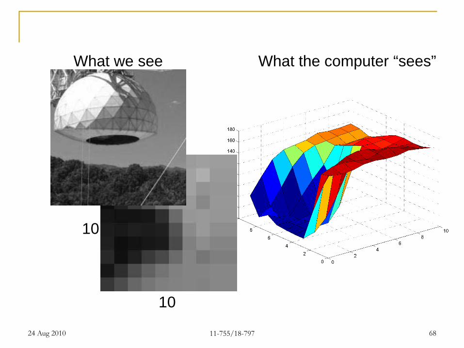
10
10
What we see What the computer “sees”
24 Aug 2010 11-755/18-797 68
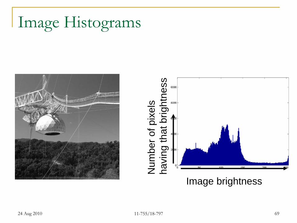
Image Histograms
Image brightness
Num
ber o
f pix
els
havi
ng th
at b
right
ness
24 Aug 2010 11-755/18-797 69
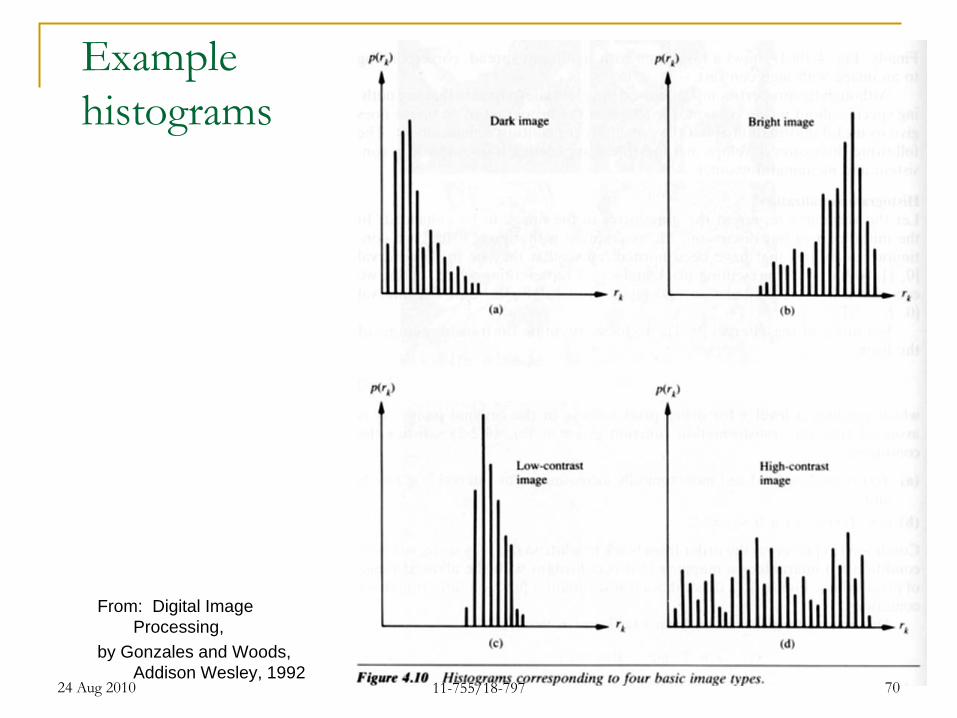
Example histograms
From: Digital Image Processing,
by Gonzales and Woods, Addison Wesley, 1992
24 Aug 2010 11-755/18-797 70

Pixel operations New value is a function of the old value
Tonescale to change image brightness Threshold to reduce the information in an image Colorspace operations
24 Aug 2010 11-755/18-797 71

J=1.5*I
24 Aug 2010 11-755/18-797 72

J=0.5*I
24 Aug 2010 11-755/18-797 73

J=uint8(0.75*I)
24 Aug 2010 11-755/18-797 74
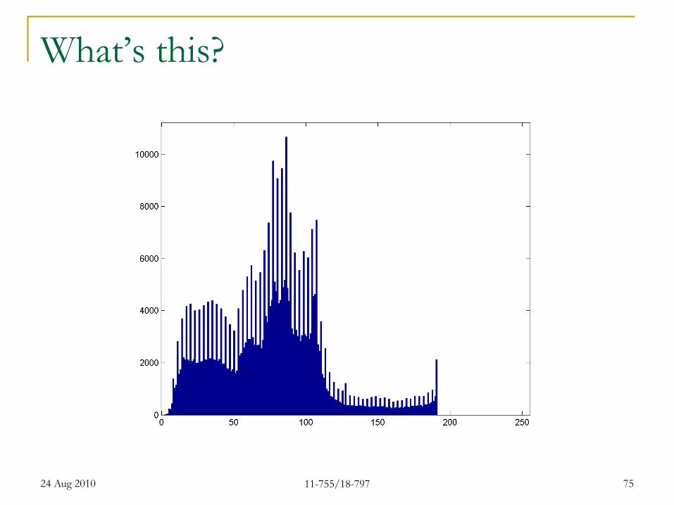
What’s this?
24 Aug 2010 11-755/18-797 75

Non-Linear Darken
24 Aug 2010 11-755/18-797 76
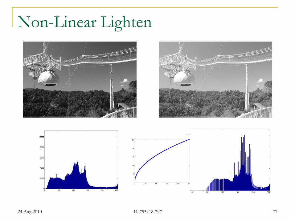
Non-Linear Lighten
24 Aug 2010 11-755/18-797 77

Linear vs. Non-Linear
24 Aug 2010 11-755/18-797 78
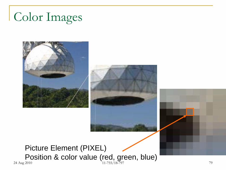
Picture Element (PIXEL)Position & color value (red, green, blue)
Color Images
24 Aug 2010 11-755/18-797 79

RGB Representation
original
R
B
G
R
B
G
24 Aug 2010 11-755/18-797 80

RGB Manipulation Example: Color Balance
original
R
B
G
R
B
G
24 Aug 2010 11-755/18-797 81
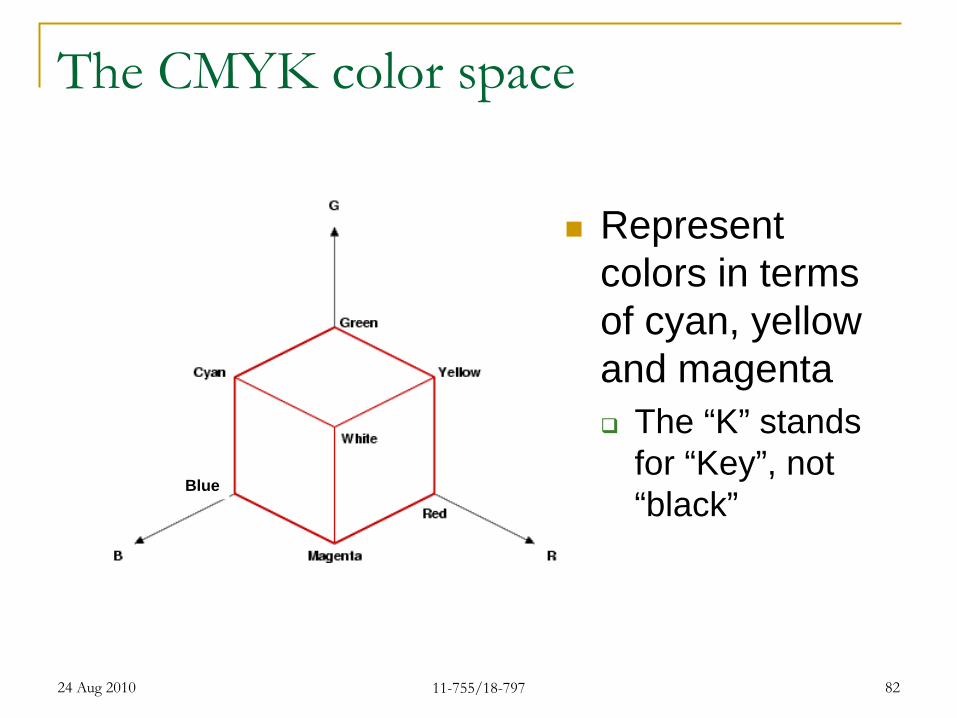
The CMYK color space
Represent colors in terms of cyan, yellow and magenta The “K” stands
for “Key”, not “black”
Blue
24 Aug 2010 11-755/18-797 82

CMYK is a subtractive representation
RGB is based on composition, i.e. it is an additive representation Adding equal parts of red, green and blue creates white
CMYK is based on masking, i.e. it is subtractive The base is white Masking it with equal parts of C, M and Y creates Black Masking it with C and Y creates Green
Yellow masks blue Masking it with M and Y creates Red
Magenta masks green Masking it with M and C creates Blue
Cyan masks green Designed specifically for printing
As opposed to rendering What happens when you mix red, green and blue paint?
Clue – paint colouring is subtractive..24 Aug 2010 11-755/18-797 83
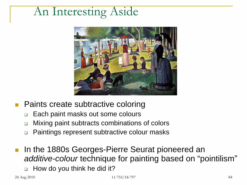
An Interesting Aside
Paints create subtractive coloring Each paint masks out some colours Mixing paint subtracts combinations of colors Paintings represent subtractive colour masks
In the 1880s Georges-Pierre Seurat pioneered an additive-colour technique for painting based on “pointilism” How do you think he did it?
24 Aug 2010 11-755/18-797 84
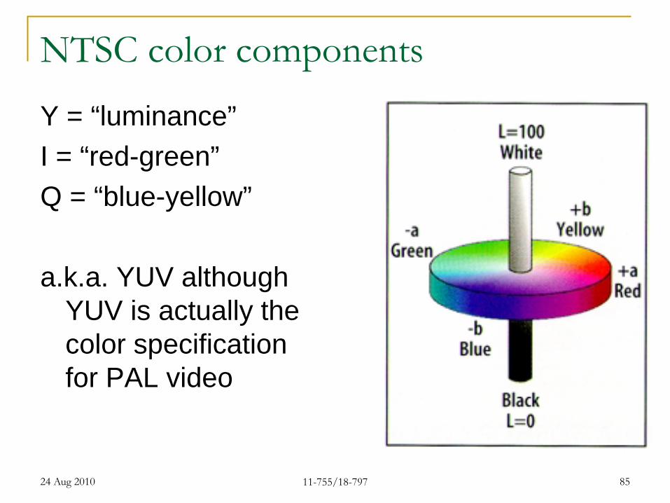
NTSC color components
Y = “luminance” I = “red-green” Q = “blue-yellow”
a.k.a. YUV although YUV is actually the color specification for PAL video
24 Aug 2010 11-755/18-797 85
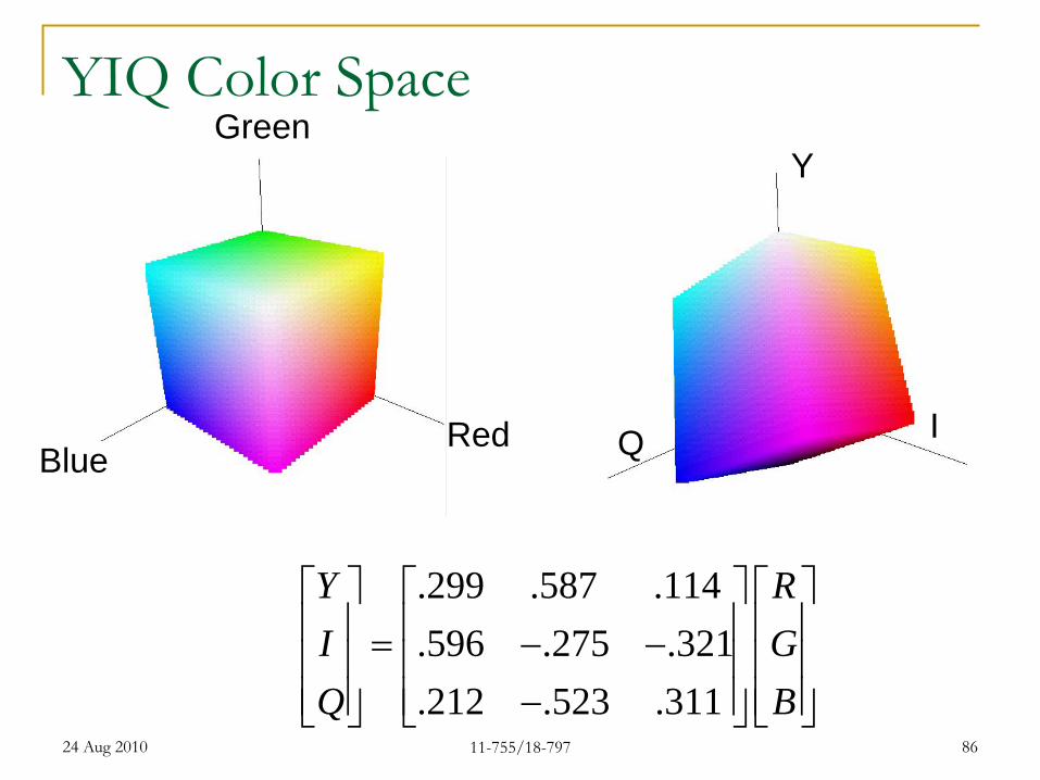
YIQ Color Space
.299 .587 .114
.596 .275 .321
.212 .523 .311
Y RI GQ B
= − − −
Red
Green
BlueIQ
Y
24 Aug 2010 11-755/18-797 86

Color Representations
Y value lies in the same range as R,G,B ([0,1]) I is to [-0.59 0.59] Q is limited to [-0.52 0.52] Takes advantage of lower human sensitivity to I and
Q axes
R
G
B
Y
IQ
24 Aug 2010 11-755/18-797 87

YIQ Top: Original image Second: Y Third: I (displayed as red-cyan) Fourth: Q (displayed as green-
magenta) From http://wikipedia.org/
Processing (e.g. histogram equalization) only needed on Y In RGB must be done on all three
colors. Can distort image colors A black and white TV only needs Y
24 Aug 2010 11-755/18-797 88

Bandwidth (transmission resources) for the components of the television signal
0 1 2 3 4
ampl
itude
frequency (MHz)
Luminance Chrominance
Understanding image perception allowed NTSC to add color to the black and white television signal. The eye is more sensitive to I than Q, so lesser bandwidth is needed for Q. Both together used much less than Y, allowing for color to be added for minimal increase in transmission bandwidth.
24 Aug 2010 11-755/18-797 89

Hue, Saturation, Value
The HSV Colour Model By Mark Roberts http://www.cs.bham.ac.uk/~mer/colour/hsv.html
V = [0,1], S = [0,1]H = [0,360]
Blue
24 Aug 2010 11-755/18-797 90
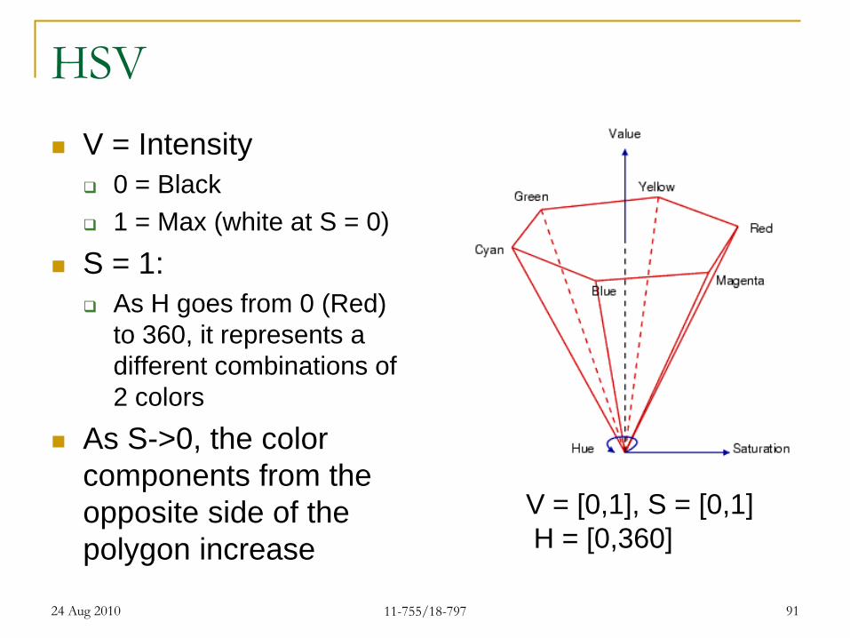
HSV V = Intensity
0 = Black 1 = Max (white at S = 0)
S = 1: As H goes from 0 (Red)
to 360, it represents a different combinations of 2 colors
As S->0, the color components from the opposite side of the polygon increase
V = [0,1], S = [0,1]H = [0,360]
24 Aug 2010 11-755/18-797 91
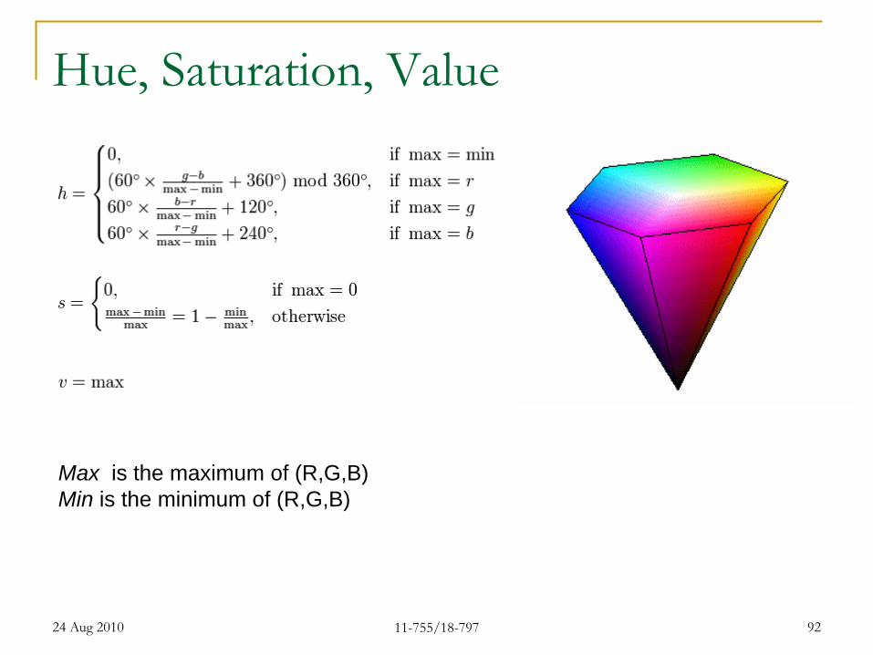
Hue, Saturation, Value
Max is the maximum of (R,G,B)Min is the minimum of (R,G,B)
24 Aug 2010 11-755/18-797 92

HSV Top: Original image Second H (assuming S = 1, V = 1) Third S (H=0, V=1) Fourth V (H=0, S=1)
H
S
V
24 Aug 2010 11-755/18-797 93

Quantization and Saturation Captured images are typically quantized to N-bits Standard value: 8 bits 8-bits is not very much < 1000:1 Humans can easily accept 100,000:1 And most cameras will give you 6-bits anyway…
24 Aug 2010 11-755/18-797 94

Saturation
24 Aug 2010 11-755/18-797 95

Processing Colour Images
Typically work only on the Grey Scale image Decode image from whatever representation to
RGB GS = R + G + B
The Y of YIQ may also be used Y is a linear combination of R,G and B
For specific algorithms that deal with colour, individual colours may be maintained Or any linear combination that makes sense may
be maintained.
24 Aug 2010 11-755/18-797 96
Reference Info
Many books Digital Image Processing, by Gonzales and
Woods, Addison Wesley, 1992 Computer Vision: A Modern Approach, by David
A. Forsyth and Jean Ponce Spoken Language Processing: A Guide to Theory,
Algorithm and System Development, by Xuedong Huang, Alex Acero and Hsiao-Wuen Hon
24 Aug 2010 11-755/18-797 97