Embed Size (px)
Citation preview
SIGNATURE COCYCLES ON THE MAPPING CLASS GROUP ANDSYMPLECTIC GROUPS
DAVE BENSON, CATERINA CAMPAGNOLO, ANDREW RANICKI, AND CARMEN ROVI
Abstract. Werner Meyer constructed a cocycle in H2(Sp(2g,Z);Z) which computes thesignature of a closed oriented surface bundle over a surface, with fibre a surface of genus g.By studying properties of this cocycle, he also showed that the signature of such a surfacebundle is a multiple of 4. In this paper, we study signature cocycles both from the geometricand algebraic points of view. We present geometric constructions which are relevant to thesignature cocycle and provide an alternative to Meyer’s decomposition of a surface bundle.Furthermore, we discuss the precise relation between the Meyer and Wall-Maslov index. Themain theorem of the paper, Theorem 7.2, provides the necessary group cohomology resultsto analyze the signature of a surface bundle modulo any integer N . Using these results, weare able to give a complete answer for N = 2, 4, and 8, and based on a theorem of Deligne,we show that this is the best we can hope for using this method.
Introduction
Given an oriented 4-manifold M with boundary, let σ(M) ∈ Z be the signature of M .As usual, let Σg be the standard closed oriented surface of genus g. For the total space Eof a surface bundle Σg → E → Σh, it is known from the work of Meyer [29] that σ(E) isdetermined by a cohomology class [τg] ∈ H2(Sp(2g,Z);Z), and that both σ(E) and [τg] aredivisible by four. This raises the question of further divisibility by other multiples of two.
Indeed, the higher divisibility of its signature is strongly related to the monodromy ofthe surface bundle: it is known since the work of Chern, Hirzebruch and Serre [11] thattrivial monodromy in Sp(2g,Z) implies signature 0. Rovi [33] showed that monodromy inthe kernel of Sp(2g,Z) → Sp(2g,Z/4) implies signature divisible by 8, and very recentlyBenson [4] proved that the monodromy lying in the even bigger theta subgroup Spq(2g,Z)implies signature divisible by 8. This settled a special case of a conjecture by Klaus andTeichner (see the introduction of [18]), namely that if the monodromy lies in the kernel ofSp(2g,Z)→ Sp(2g,Z/2), the signature is divisible by 8. This result also follows by work ofGalatius and Randal-Williams [15], by completely different methods.
Let us briefly recall the more general importance of the divisibility of the signature inthe topology and geometry of manifolds: 4k-dimensional compact oriented hyperbolic man-ifolds have signature equal to 0, 4-dimensional smooth spin closed manifolds have signaturedivisible by 16.
In the first sections of this paper, we start by giving a review of essential notions: inparticular, we review forms, signature, Novikov additivity and Wall non-additivity of thesignature, and include a discussion of the relation between the Meyer cocycle and the Maslovcocycle. Furthermore, we describe the geometric constructions relevant to the signature
2010 Mathematics Subject Classification. 20J06 (primary) ; 55R10, 20C33 (secondary).1
cocycle. In [29], Meyer constructs his cocycle by decomposing the base space of the surfacebundle into pairs of pants and then using Novikov additivity of the signature. Here wepresent an alternative construction in Figure 9.
In Section 3 we explain the cohomology of Lie groups seen as discrete groups and itsrelationship to their usual cohomology. Specifically, in Section 4, we study the case of theunit circle seen as a discrete group and give expressions for the restriction of the Meyer andMaslov cocycles in this setting.
In [5], we constructed a cohomology class in the second cohomology group of a finitequotient H of Sp(2g,Z) that computes the mod 2 reduction of the signature divided by 4 fora surface bundle over a surface.
The main theorem of this paper, Theorem 7.2, presents an extensive study of the inflationsand restrictions of the Meyer class to various quotients of the symplectic group. It providesthe necessary group cohomology results to analyze the signature of a surface bundle moduloany integer N . Its upshot can be summarized in the diagram below, valid for g ≥ 4, whichillustrates the connection between Meyer’s cohomology class, on the bottom right, and thecentral extension H of H regarded as a cohomology class, on the top left. The group H isthe smallest quotient of the symplectic group that contains the cohomological informationabout the signature modulo 8 of a surface bundle over a surface.
Z/2 = H2(H;Z/2)∼=
//
∼=
H2(H;Z/8) = Z/2∼=
Z/2 = H2(Sp(2g,Z/4);Z/2)∼=//
∼=
H2(Sp(2g,Z/4);Z/8) = Z/2
4
Z/2 = H2(Sp(2g,Z);Z/2)4// H2(Sp(2g,Z);Z/8) = Z/8
Z = H2(Sp(2g,Z);Z)4
//
OOOO
H2(Sp(2g,Z);Z) = Z
OOOO
In these new computations, we focus on g ≥ 2. Our reasons for that are threefold: wheng = 1, 2, the signature of surface bundles over surfaces is 0 anyway [29], so that we do notneed these cases for our purposes. But while g = 2 compares in a reasonable way to thehigher genera, the cohomology of Sp(2,Z) and its quotients behave quite differently: eventhough part of the properties we investigate are shared by all g’s, the common pattern ismore often lost when g = 1. Finally, as it happens that Sp(2,Z) = SL(2,Z), the cohomologyof this group has been studied in depth in other contexts [1, 6, 21].
We apply Theorem 7.2 to the study of the signature modulo N for surface bundles. Theoutcome is the following:
Theorem 7.3. Let g > 4 and Q be a finite quotient of Sp(2g,Z). If c ∈ H2(Q;Z/N) is acohomology class such that for the monodromy χ : π1(Σh)→ Sp(2g,Z) of any surface bundleΣg → E → Σh we have
σ(E) = −〈χ∗p∗(c), [Σh]〉 ∈ Z/N,2
then N = 2, 4, or 8. If N = 2 or 4, the value 〈χ∗p∗(c), [Σh]〉 ∈ Z/N is always 0. Herep : Sp(2g,Z)→ Q denotes the quotient map.
Furthermore, we generalize this result to arbitrary coefficient rings and show that anycohomology class on a finite quotient of the symplectic group yields at most 2-valued infor-mation on the signature of a surface bundle over a surface since it lies in the 2-torsion ofthe arbitrary coefficient ring. This explains the choice of the study of the signature modulo8 by showing that it is the best information a cohomology class on a finite quotient of thesymplectic group can provide.
The paper is complemented by three appendices: Appendix A contains background on thehomology and cohomology of discrete groups. Appendix B collects computations of the firstand second homology and cohomology of the mapping class group, the symplectic group andsome of its quotients, as will be often used in the main sections. Finally, Appendix C is abiography of W. Meyer by W. Scharlau.
Acknowledgements. The authors thank Christophe Pittet for a helpful correspondenceabout Theorem 3.5. Campagnolo acknowledges support by the Swiss National Science Foun-dation, grant number PP00P2-128309/1, and by the German Science Foundation via theResearch Training Group 2229, under which this research was started and completed.
The writing of this paper was overshadowed by the death of Andrew Ranicki in February2018. With deep sorrow, we dedicate this work to his memory.
1. The signature
1.1. Forms. Let R be a commutative ring. The dual of an R-module V is the R-module
V ∗ = HomR(V,R) .
The dual of an R-module morphism f : V → W is the R-module morphism
f ∗ : W ∗ −→ V ∗ ; g 7−→ (x 7−→ g(f(x))) .
As usual, we have an isomorphism of abelian groups
V ∗ ⊗R V ∗ −→ HomR(V, V ∗) ; f ⊗ g 7−→ (x 7−→ (y 7−→ f(x)g(y))) .
If V is f.g. free then so is V ∗, and the natural R-module morphism
V −→ V ∗∗ ; x 7−→ (f 7−→ f(x))
is an isomorphism, in which case it will be used to identify V = V ∗∗.A form (V, b) over R is a f.g. free R-module V together with a bilinear pairing b : V ×V →
R, or equivalently the R-module morphism
b : V −→ V ∗ ; x 7−→ (y 7−→ b(x, y)) .
A morphism of forms f : (V, b)→ (W, c) over R is an R-module morphism f : V → W suchthat
f ∗cf = b : V −→ V ∗
or equivalently
c(f(x), f(y)) = b(x, y) ∈ R (x, y ∈ V ) .3
For ε = ±1 a bilinear form (V, b) is ε-symmetric if
b(y, x) = εb(x, y) ∈ R (x, y ∈ V ) ,
or equivalently εb∗ = b ∈ HomR(V, V ∗). For ε = 1 the form is symmetric; for ε = −1 theform is symplectic.
Given a form (V, b) over R the orthogonal of a submodule L ⊆ V is the submodule
L⊥ = x ∈ V | b(x, y) = 0 ∈ R for all y ∈ L .The radical of (V, b) is the orthogonal of V
V ⊥ = x ∈ V | b(x, y) = 0 ∈ R for all y ∈ V .The form (V, b) is nonsingular if the R-module morphism
b : V −→ V ∗ ; x 7−→ (y 7−→ b(x, y))
is an isomorphism, in which case V ⊥ = 0.A lagrangian of a nonsingular form (V, b) is a f.g. free direct summand L ⊂ V such that
L⊥ = L, or equivalently such that the sequence
0 // Lj// V
j∗b// L∗ // 0
is exact, with j : L → V the inclusion. The metabolic ε-symmetric form defined for anyε-symmetric form (L∗, λ) by
Hε(L) = (L⊕ L∗,(
0 1ε λ
))
is a nonsingular ε-symmetric form over R with lagrangian L.
Proposition 1.1. (i) A nonsingular ε-symmetric form over R admits a lagrangian if andonly if it is isomorphic to Hε(L∗, λ) for some ε-symmetric form (L∗, λ).(ii) For any nonsingular ε-symmetric form (V, b) over R and α ∈ Aut(V, b) the image α(L) ⊂V is a lagrangian of (V, b).(iii) For any lagrangian L of Hε(Rg) there exists α ∈ AutHε(Rg) such that L = α(Rg ⊕ 0).(iv) For any (−ε)-symmetric form (L, θ) there is defined an automorphism
α =
(1 0θ 1
): Hε(L) −→ Hε(L)
and hence a lagrangian of Hε(L)
α(L) = (x, θ(x)) ∈ L⊕ L∗ |x ∈ L .(v) For any nonsingular ε-symmetric form (V, b) over R there is defined a lagrangian of(V, b)⊕ (V,−b)
∆ = (x, x) ∈ V ⊕ V |x ∈ V .For any α ∈ Aut(V, b) the image of the diagonal lagrangian under the automorphism
1⊕ α : (V, b)⊕ (V,−b) −→ (V, b)⊕ (V,−b)
is a lagrangian of (V, b)⊕ (V,−b)
graph(α) = (1⊕ α)(∆) = (x, α(x)) |x ∈ V ⊆ V ⊕ V . 4
Example 1.2. (i) The intersection form of a 2n-dimensional manifold with boundary (M,∂M)is the (−)n-symmetric form (Hn(M,∂M), bM) over R
bM : Hn(M,∂M ;R)×Hn(M,∂M ;R) −→ R ; (x, y) 7−→ 〈x ∪ y, [M ]〉with radical
Hn(M,∂M ;R)⊥ = ker (Hn(M,∂M ;R) −→ Hn(M ;R)) .
If M is closed then (Hn(M ;R), bM) is nonsingular.(ii) If (N, ∂N) is a (2n+ 1)-dimensional manifold with boundary then
ker (Hn(∂N ;R) −→ Hn(N ;R)) ⊆ Hn(∂N ;R)
is a lagrangian of (Hn(∂N ;R), b∂N).
1.2. Signature.
Definition 1.3. The signature of a symmetric form (V, b) over R is defined as usual by
σ(V, b) = dimRV+ − dimRV− ∈ Z
for any decomposition
(V, b) = (V+, b+)⊕ (V−, b−)⊕ (V0, 0)
with (V+, b+) (resp. (V−, b−)) positive (resp. negative) definite.
Definition 1.4. The signature of a 4k-dimensional manifold with boundary (W,∂W ) is
σ(W ) = σ(H2(W,∂W ;R), bW ) ∈ Z .
We shall only be concerned with the case k = 1.
Proposition 1.5. (Novikov additivity of the signature)The signature of the union W1 ∪W2 of 4k-dimensional manifolds with boundary along thewhole boundary components is
σ(W1 ∪W2) = σ(W1) + σ(W2) .
The following construction is central to the computation of the signature of singular sym-metric forms over R, such as arise from 4-dimensional manifolds with boundary.
Proposition 1.6. (Wall [39]) Let (V, b) be a nonsingular ε-symmetric form over R, and letj1 : L1 → V , j2 : L2 → V , j3 : L3 → V be the inclusions of three lagrangians such that theR-module
∆ = ∆(L1, L2, L3) = (a, b, c) ∈ L1 ⊕ L2 ⊕ L3 | a+ b+ c = 0 ∈ V = ker ((j1 j2 j3) : L1 ⊕ L2 ⊕ L3 −→ V )
is f.g. free.(i) The form (∆, a) over R defined by
a =
0 j∗1bj2 00 0 00 0 0
: ∆×∆ −→ R ;
((a, b, c), (a′, b′, c′)) 7−→ b(b, a′) = −b(c, a′) = b(c, b′) ,5
is (−ε)-symmetric, with radical
∆⊥ =(L1 ∩ L2)⊕ (L2 ∩ L3)⊕ (L3 ∩ L1)
L1 ∩ L2 ∩ L3
⊆ ∆ .
(ii) The (−ε)-symmetric form
(∆′, a′) =
(ker ((j∗3bj1 j
∗3bj2) : L1 ⊕ L2 −→ L∗3) ,
(0 j∗1bj2
0 0
))is such that there is defined an isomorphism f : (∆, a) ∼= (∆′, a′) with
f : ∆ −→ ∆′ = (a, b) ∈ L1 ⊕ L2 | a+ b ∈ L3 ; (a, b, c) 7−→ (a, b) .
(iii) If j∗3bj2 : L2 → L∗3 is an isomorphism there is defined an isomorphism of (−ε)-symmetricforms (
1−(j∗3bj2)−1(j∗3bj1)
):(L1,−(j∗1bj2)(j∗3bj2)−1(j∗3bj1)
) ∼=// (∆′, a′) .
Proof. (i) See Wall [39].(ii)+(iii) Immediate from (i).
Remark 1.7. The construction appeared independently later in the work of Leray [24],clarifying earlier work of Maslov [27].
Definition 1.8. (Maslov [27], Wall [39], Leray [24]) The Wall–Maslov index for any con-figuration of three lagrangians L1, L2, L3 of a nonsingular symmetric form (V, b) over R isdefined to be the signature
τ(L1, L2, L3) = σ(∆(L1, L2, L3), a) ∈ Z .
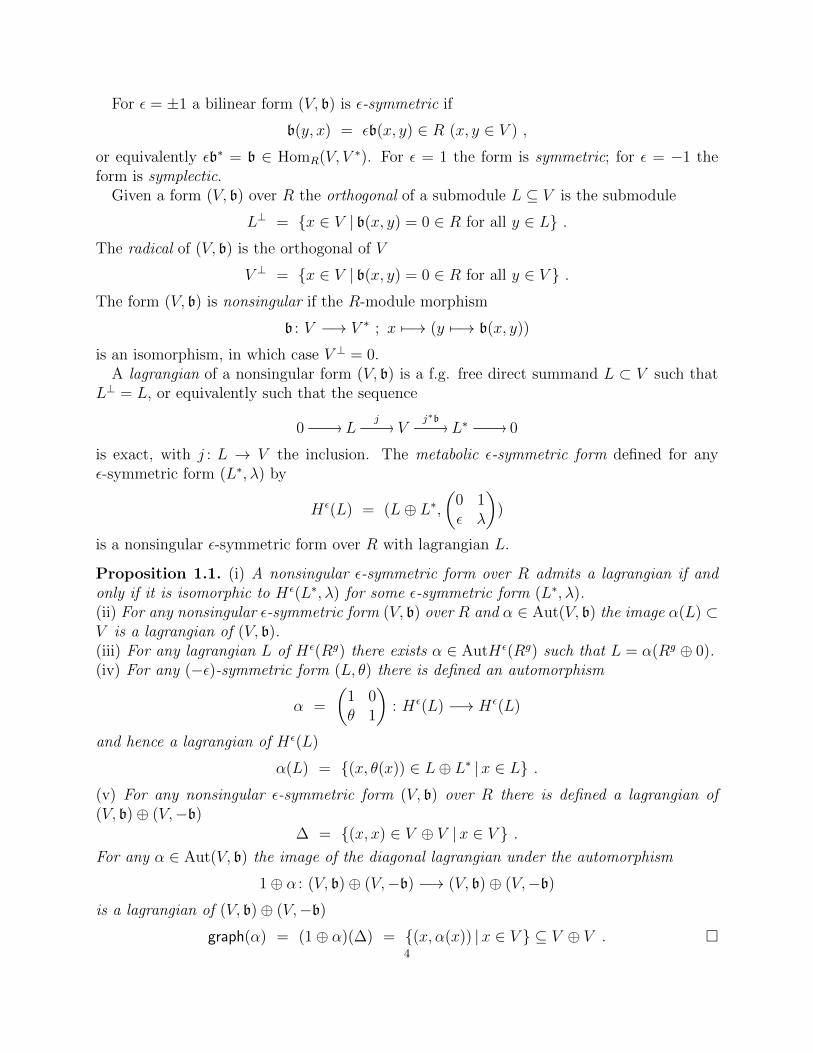
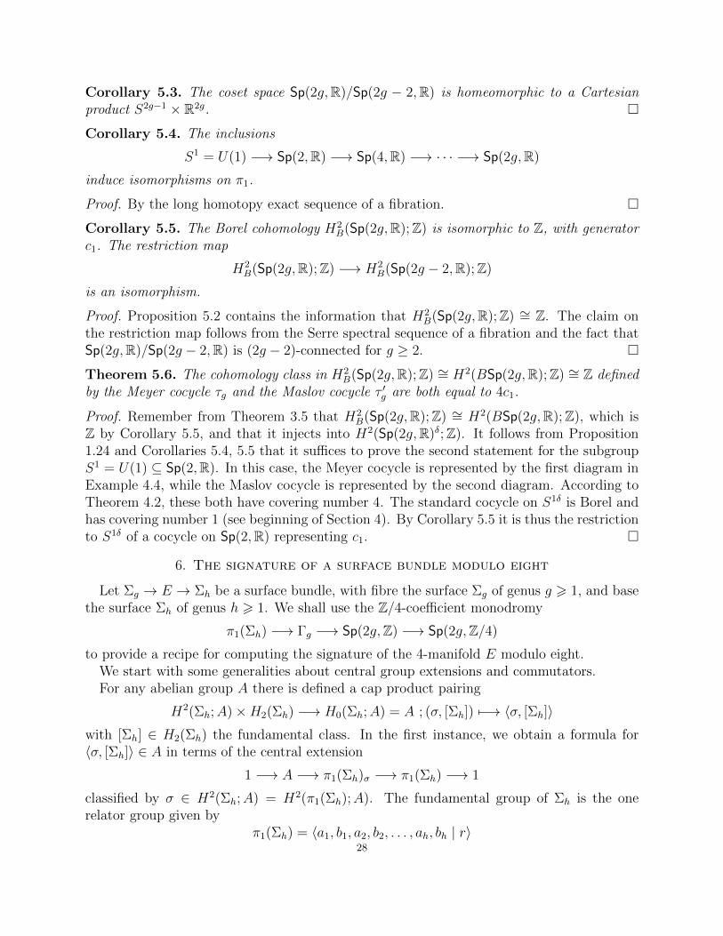
Proposition 1.9. (Wall non-additivity of the signature [39]) Let (W,∂W ) be a 4-dimensionalmanifold with boundary which is a union of three codimension 0 submanifolds with boundary(Wi, ∂+Wi t ∂−Wi), i = 1, 2, 3,
(W,∂W ) = (W1 ∪W2 ∪W3, ∂−W1 t ∂−W2 t ∂−W3)
such that W1 ∩W2, W2 ∩W3 and W3 ∩W1 are three 3-manifolds with the same boundarysurface
W1 ∩W2 ∩W3 = ∂(W1 ∩W2) = ∂(W2 ∩W3) = ∂(W3 ∩W1) = Σ .
The signature of (W,∂W ) is
σ(W ) = σ(W1) + σ(W2) + σ(W3)− σ(∆(L1, L2, L3)) ∈ Z
with the three lagrangians of (H1(Σ;R), bΣ)
L1 = ker(H1(Σ;R) −→ H1(W2 ∩W3;R)
),
L2 = ker(H1(Σ;R) −→ H1(W3 ∩W1;R)
),
L3 = ker(H1(Σ;R) −→ H1(W1 ∩W2;R)
).
Remark 1.10. The Novikov additivity of the signature is the special case of the Wall non-additivity of the signature when the glueing is done along the whole boundary.
6
α
α
α
α
α γ
γα α
α
Idα
βαβ
αβ
γ
γαβ
γβ
β β
β
β
β
α β
β
Id
Id
Id
Id
Id
double-mappingtorus-blownup
T(α, β) T(αβ, γ)
T(α, βγ)
T(β, γ)
W
3
Σ ∂−W1 ∂−W2
∂−W3
W1 W2
W3
Σ
Figure 1. The union W1 ∪W2 ∪W3
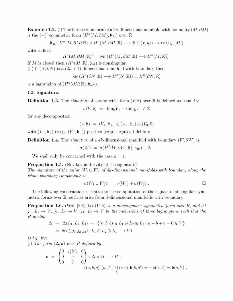
Definition 1.11. (i) Let N1, N2 be two 3-manifolds with the same boundary
∂N1 = ∂N2 = Σg ,
i.e. such that there are given embeddings ij : Σg → Nj (j = 1, 2) with ij(Σg) = ∂Nj. Thetwisted double is the closed 3-dimensional manifold
D(N1, N2, i1, i2) = (N1 tN2)/i1(x) ∼ i2(x) |x ∈ Σg .
(ii) Let N1, N2, N3 be three 3-manifolds with the same boundary
∂N1 = ∂N2 = ∂N2 = Σ ,
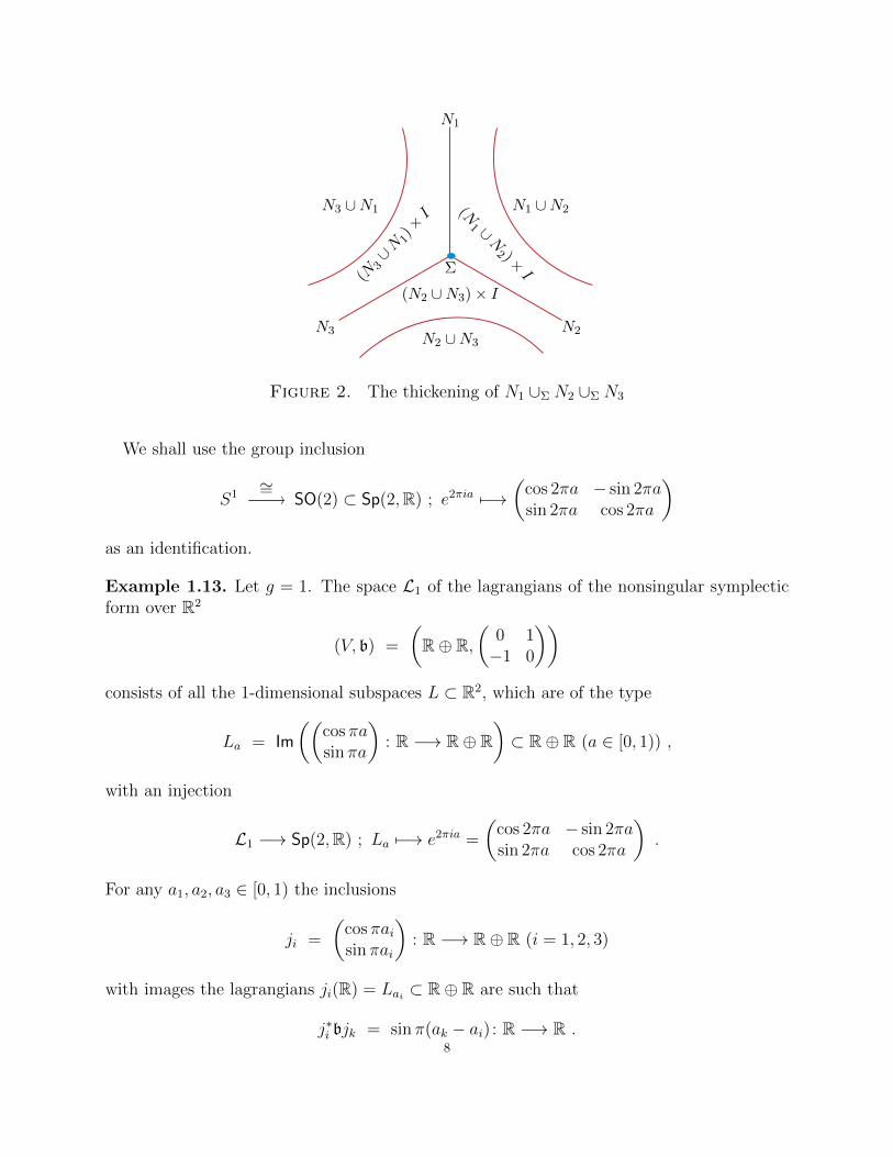
i.e. such that there are given embeddings ij : Σ → Nj (j = 1, 2, 3) with ij(Σ) = ∂Nj. Thethickening of the stratified set
N1 ∪Σ N2 ∪Σ N3 = (N1 tN2 tN3)/i1(x) ∼ i2(x) ∼ i3(x) |x ∈ Σ
is the 4-dimensional manifold with boundary
(W (N1, N2, N3,Σ), ∂W (N1, N2, N3,Σ))
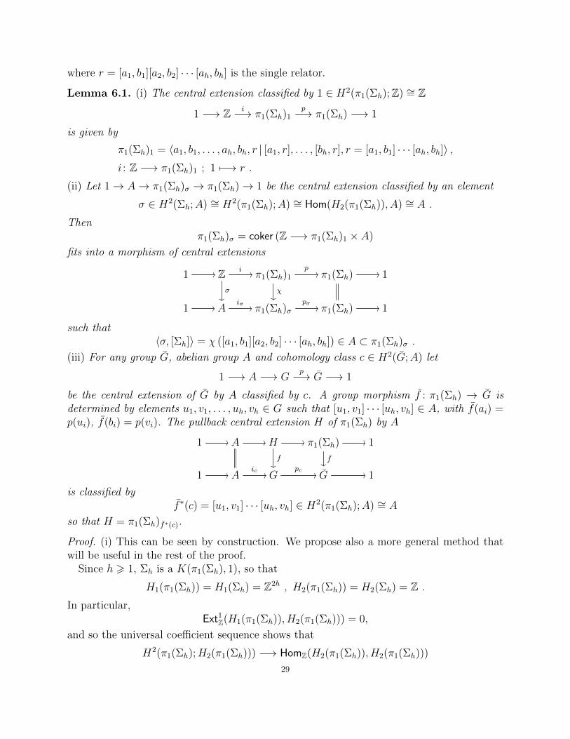
= (D(N1, N2, i1, i2)× I ∪D(N2, N3, i2, i3)× I ∪D(N3, N1, i3, i1)× I,D(N1, N2, i1, i2) tD(N2, N3, i2, i3) tD(N3, N1, i3, i1)) .
Proposition 1.12. As in Definition 1.11 (ii), let N1, N2, N3 be 3-dimensional manifoldswith the same boundary
∂N1 = ∂N2 = ∂N3 = Σ .
The nonsingular symplectic intersection form over R
(V, b) =(H1(Σ;R), bΣ
)has three lagrangians
Li = Im(H1(Ni;R) −→ H1(Σ;R)
)(i = 1, 2, 3),
such that the signature of the thickening W (N1, N2, N3,Σ) is given by
σ (W (N1, N2, N3,Σ)) = −τ(L1, L2, L3) ∈ Z .
Proof. This is a special case of Proposition 1.9. 7
Σ
N1
N2N3
N3 ∪N1
(N3∪N
1)×I
N1 ∪N2(N1 ∪N
2 )×I
N2 ∪N3
(N2 ∪N3)× I
Figure 2. The thickening of N1 ∪Σ N2 ∪Σ N3
We shall use the group inclusion
S1∼=// SO(2) ⊂ Sp(2,R) ; e2πia 7−→
(cos 2πa − sin 2πasin 2πa cos 2πa
)as an identification.
Example 1.13. Let g = 1. The space L1 of the lagrangians of the nonsingular symplecticform over R2
(V, b) =
(R⊕ R,
(0 1−1 0
))consists of all the 1-dimensional subspaces L ⊂ R2, which are of the type
La = Im
((cos πasin πa
): R −→ R⊕ R
)⊂ R⊕ R (a ∈ [0, 1)) ,
with an injection
L1 −→ Sp(2,R) ; La 7−→ e2πia =
(cos 2πa − sin 2πasin 2πa cos 2πa
).
For any a1, a2, a3 ∈ [0, 1) the inclusions
ji =
(cosπaisin πai
): R −→ R⊕ R (i = 1, 2, 3)
with images the lagrangians ji(R) = Lai ⊂ R⊕ R are such that
j∗i bjk = sin π(ak − ai) : R −→ R .8
As in Lemma 1.6 (ii) there is defined an isomorphism of symmetric forms over R
f : (∆(La1 , La2 , La3), a)
=
ker
((cos πa1 cosπa2 cosπa3
sinπa1 sin πa2 sin πa3
): R⊕ R⊕ R −→ R⊕ R
),
0 1 00 0 00 0 0
∼=// (∆′(La1 , La2 , La3), a
′)
=
(ker((
sin π(a1 − a3) sin π(a2 − a3))
: R⊕ R −→ R),
(0 sin π(a2 − a1)0 0
)).
If a1, a2, a3 are not all distinct then b = 0, and τ(La1 , La2 , La3) = 0. If a2 6= a3 then Lemma1.6 (iii) gives an isomorphism(
1−(j∗3bj2)−1(j∗3bj1)
):(R,−(j∗1bj2)(j∗3bj2)−1(j∗3bj1)
) ∼=// (∆′, a′) .
It follows that for any a1, a2, a3 ∈ [0, 1) the Wall-Maslov index is
τ(La1 , La2 , La3) = τ(∆(La1 , La2 , La3), a)
= τ(∆′(La1 , La2 , La3), a′)
= τ(R,− sin π(a1 − a2) sinπ(a2 − a3) sinπ(a3 − a1))
= −sign(sinπ(a1 − a2) sinπ(a2 − a3) sinπ(a3 − a1)) .
Lemma 1.14. If α ∈ Sp(2g,R) then τ(α(L1), α(L2), α(L3)) = τ(L1, L2, L3).
Proof. This is clear from the definition.
Lemma 1.15. If L1, L2, L3, L4 are lagrangians in R2g then
τ(L1, L2, L3)− τ(L1, L2, L4) + τ(L1, L3, L4)− τ(L2, L3, L4) = 0.
Proof. See for example Py [32, Theoreme (2.2.1)].
Now suppose that the symplectic form over R
(R2g+2, b′) = (R2g, b)⊕ (R⊕ R, 〈 , 〉)
is formed from (R2g, b) by adjoining new basis elements vg+1 and wg+1 with 〈vg+1, vg+1〉 = 0,〈wg+1, wg+1〉 = 0 and 〈vg+1, wg+1〉 = 1. Then given any lagrangian L in (R2g, b), we may
form the lagrangian L = L⊕ Rvg+1 in (R2g+2, b′).
Lemma 1.16. Setting ∆ = ∆(L1, L2, L3), we have an isomorphism
(∆, a) = (∆, a)⊕ (Rvg+1, 0) .
In particular, we have
τ(L1, L2, L3) = τ(L1, L2, L3).
Proof. The space ∆ consists of vectors
(a, b, c) = (a+ λvg+1, b+ µvg+1, c+ νvg+1)9
with (a, b, c) ∈ ∆ and λ+ µ+ ν = 0, and the symmetric form (∆, a) is given by
b((a, b, c), (a′, b′, c′)) = a(b, a′)
= a(b, a′) = b((a, b, c), (a′, b′, c′)) .
Lemma 1.17. Let (V, b) be a nonsingular symplectic form over R.(i) The graph of an automorphism α : (V, b)→ (V, b) is a lagrangian of (V ⊕ V, b⊕−b)
graph(α) = Im
((1α
): V −→ V ⊕ V
)⊂ V ⊕ V .
(ii) For any automorphisms αi : (V, b)→ (V, b) (i = 1, 2, 3) let
ji =
(1αi
): (V, 0) −→ (V ⊕ V, b⊕−b)
be the inclusions of the three graph lagrangians. For i 6= k
j∗i (b⊕−b)jk = b− α∗i bαk = b(1− α−1i αk) : V −→ V ∗ ,
so that
(∆′(graph(α1), graph(α2), graph(α3)), a′)
=
(ker((1− α−1
3 α1 1− α−13 α2) : V ⊕ V −→ V
),
(0 b(1− α−1
1 α2)0 0
)).
If one of 1 − α−1i αk is 0 then b′ = 0 and τ(graph(α1), graph(α2), graph(α3)) = 0. If 1 −
α−13 α2 : V → V is an isomorphism there is defined an isomorphism of symmetric forms(
1−(b− α∗3bα2)−1(b− α∗3bα1)
): (V,−(b− α∗1bα2)(b− α∗3bα2)−1(b− α∗3bα1))
∼=// (∆′(graph(α1), graph(α2), graph(α3)), b′) ,
so thatτ(graph(α1), graph(α2), graph(α3))
= τ(V,−(b− α∗1bα2)(b− α∗3bα2)−1(b− α∗3bα1))
= τ(V,−b(1− α−11 α2)(1− α−1
3 α2)−1(1− α−13 α1)) .
Proof. (i) By construction.(ii) Apply Lemma 1.6.
Note that the graph of any element α ∈ Sp(2g,R)
graph(α) = (x, α(x)) |x ∈ R2g ⊂ R2g ⊕ R2g
is a lagrangian of the symplectic form(R2g ⊕ R2g, ((x, y), (x′, y′)) 7−→ 〈x, x′〉 − 〈y, y′〉
),
and that the signature of the double mapping torus (§2.3 below) is
σ(T (α, β)) = −τ(graph(1), graph(α), graph(αβ)) ∈ Z .10
In what follows, when we write Sp(2g,R)δ we mean the same group Sp(2g,R), but with thediscrete topology. For more details on the cohomology of Lie groups with discrete topologysee Section 3.
Definition 1.18. The Meyer cocycle τg : Sp(2g,R)δ × Sp(2g,R)δ → Z is defined by
τg(α, β) = τ(graph(1), graph(α), graph(αβ)).
Remark 1.19. It follows from Lemma 1.15 that τg is a cocycle on Sp(2g,R)δ. By Lemma1.14 we have
τg(α, β) = τ(graph(α−1), graph(1), graph(β)).
So the subspace ∆ consists of triples((x, α−1(x)), (−x− y,−x− y), (y, β(y))
)with x, y ∈ R2g such that α−1(x) + β(y) = x+ y. Thus ∆ is isomorphic to the space
(x, y) ∈ R2g ⊕ R2g | (α−1 − 1)x+ (β − 1)y = 0,
with symmetric form
b ((x, y), (x′, y′)) = 〈x+ y, (1− β)y′〉 .This is the definition found in Meyer [29], except that the original cocycle was on Sp(2g,Z).
Example 1.20. Let (V, b) =
(R⊕ R,
(0 1−1 0
)), so that identifying V = C have b = −i =
e−πi/2. For a ∈ [0, 1) let
α = e2πia =
(cos 2πa − sin 2πasin 2πa cos 2πa
)∈ Aut(V, a) = Sp(2,R) ,
so that
1− α = (2 sinπa)eπi(a+1/2) = (2 sinπa)
(sinπa cos πa− cosπa sinπa
).
(i) For any a1, a2, a3 ∈ [0, 1) let αj = e2πiaj (j = 1, 2, 3). By Lemma 1.17 (ii) the Wall-Maslovindex of the graph lagrangians graph(αj) in (V ⊕ V, b⊕−b) is
τ(graph(α1), graph(α2), graph(α3))
= τ(V,−a(1− α−11 α2))(1− α−1
3 α2)−1(1− α−13 α1))
= τ(V,−e−πi/2((2 sinπ(a2 − a1))eπi(a2−a1+1/2))((2 sinπ(a2 − a3))eπi(a2−a3+1/2))−1
((2 sinπ(a1 − a3))eπi(a1−a3+1/2)))
= τ(V,−2 sinπ(a2 − a1) sinπ(a1 − a3)
sin π(a2 − a3))
= −2sign(sinπ(a1 − a2) sinπ(a2 − a3) sinπ(a3 − a1)) ∈ 0, 2,−2 .
(ii) By (i) the evaluation of the Meyer cocycle on α = e2πia, β = e2πib ∈ Sp(2,R) is
τ1(α, β) = τ(graph(1), graph(α), graph(αβ))
= −2sign(sinπa sin πb sin π(a+ b)) ∈ 0, 2,−2 .11
We now consider another cocycle τ ′g on Sp(2g,R)δ, again defined in terms of the Maslovindex. We shall see in Theorem 5.6 below that it is cohomologous to the Meyer cocycle τg,but not equal to it. (For g = 1 see Example 1.22).
Definition 1.21. The Maslov cocycle τ ′g : Sp(2g,R)δ × Sp(2g,R)δ → Z is defined as follows.
Choose a lagrangian subspace L ⊆ R2g, and set
τ ′g(α, β) = τ(L, α(L), αβ(L)).
It follows from Lemma 1.14 that this is independent of the choice of L, and that
τ ′g(α, β) = τ(α−1(L), L, β(L)).
Example 1.22. Using the inclusion
[0, 1)∼=// SO(2) ⊂ Sp(2,R) ; a 7−→ e2πia =
(cos 2πa − sin 2πasin 2πa cos 2πa
)as an identification we have that for g = 1 Example 1.20 gives the Meyer cocycle on [0, 1)to be
τ1 : [0, 1)× [0, 1) −→ Z ; (a, b) 7−→ −2sign(sinπa sin πb sinπ(a+ b)) .
The Maslov cocycle is given by
τ ′1 : [0, 1]×[0, 1] −→ Z ; (a, b) 7−→ τ(L0, L2πa, L2π(a+b)) = −sign(sin 2πa sin 2πb sin(2π(a+b))) .
The Dedekind (( ))-function is defined by
(( )) : R −→ (−1/2, 1/2) ; x 7−→ ((x)) =
x − 1/2 if x ∈ R\Z,0 if x ∈ Z,
with x ∈ [0, 1) the fractional part of x ∈ R, and is such that
2((2x))− 4((x)) = sign(sin 2πx) ,
2( ((x)) + ((y))− ((x+ y)) ) = −sign(sinπx sin πy sin π(x+ y)) .
Thus
τ1(a, b) = 4( ((a)) + ((b))− ((a+ b)) ) ,
τ ′1(a, b) = 2( ((2a)) + ((2b))− ((2a+ 2b)) ) ,
τ1(a, b)− τ ′1(a, b) = −sign( sin 2πa)− sign(sin 2πb) + sign(sin 2π(a+ b)) ∈ Z
and
[τ1] = [τ ′1] ∈ H2(Sp(2,R)δ;Z) .
(See also Example 4.4.)
Remark 1.23. Gilmer and Masbaum recall a result of Walker in [16, Theorem 8.10] thatstates in their notations that
[τ ′g]
= − [τg] for every g ≥ 1. This is because they have theconvention that τg(α, β) is the signature of the surface bundle over a pair of pants defined byα, β [16, p. 1087], while Meyer [29, p. 243] and this paper (Definition 1.18 and just above)take the opposite convention, that τg(α, β) is minus the signature of the surface bundle overa pair of pants defined by α, β.
12
Proposition 1.24. Embed R2g in R2g+2 by adjoining new basis elements vg+1 and wg+1, andconsider the corresponding embedding Sp(2g,R)δ → Sp(2g + 2,R)δ.
(i) The Maslov cocycle τ ′g+1 on Sp(2g + 2,R)δ restricts to the Maslov cocycle τ ′g on
Sp(2g,R)δ.(ii) The Meyer cocycle τg+1 on Sp(2g+2,R)δ restricts to the Meyer cocycle τg on Sp(2g,R)δ.
Proof. (i) This follows immediately from Lemma 1.16.(ii) For α ∈ Sp(2g,R)δ, the graph of α considered as an element of Sp(2g + 2,R)δ is the
direct sum of the graph of α considered as an element of Sp(2g,R)δ and graph(1) ⊂ R2⊕R2.So apply Lemma 1.16 twice.
2. Surface bundles and the mapping torus constructions
In section 2.1 we recall the classification of oriented surface bundles Σg → E → B withthe fibre Σg the standard closed surface of genus g and the base B an oriented manifold withboundary (which may be empty). We shall be particularly concerned with the constructionof surface bundles in four specific cases of the base B, in each of which E is obtained fromthe monodromy morphism π1(B) → Γg to the mapping class group of Σg by a geometricmapping torus construction:
(i) for a circle (2.2),(ii) for a pair of pants (2.3),
(iii) for a punctured torus (2.4),(iv) for a surface (2.5).
Note that when we talk about a punctured surface we mean a surface with a boundarycomponent for each puncture.
In Section 2.6 we construct a geometric cocycle τ ∈ H2(Γg; Ω4) for the oriented cobordismclass (= signature) of the total space E of a surface bundle Σg → E → B = Σh over asurface.
2.1. Classification of surface bundles. Let Homeo(Σg) be the topological group of self-homeomorphisms α : Σg → Σg, and let Homeo+(Σg) ⊂ Homeo(Σg) be the subgroup of theorientation-preserving self-homeomorphisms. A surface bundle Σg → E → B is oriented ifthe manifolds B,F are oriented and the structure group of the bundle is Homeo+(Σg), sothat E is also an oriented manifold. We shall only be considering oriented surface bundles.
Let EHomeo+(Σg) be a contractible space with a free Homeo+(Σg)-action, so that thesurface bundle over the classifying space BHomeo+(Σg) = EHomeo+(Σg)/Homeo+(Σg)
Σg −→ EHomeo+(Σg)×Homeo+(Σg) Σg −→ BHomeo+(Σg)
is universal. We shall only consider Homeo+(Σg) for g > 2, when the connected com-ponents are contractible. The set of connected components is the mapping class groupΓg = π0Homeo+(Σg), the discrete group of isotopy classes of orientation preserving home-omorphisms α : Σg → Σg, and the forgetful map BHomeo+(Σg) → BΓg is a homotopyequivalence.
13
Proposition 2.1. (Farb and Margalit [14, pp. 154–155]) For g ≥ 2, every surface bundleΣg → E → B is isomorphic to the pullback of the universal surface bundle along a mapB → BΓg, with the monodromy defining a bijective correspondence
isomorphism classes of surface bundles Σg → E → B ≈
[B,BHomeo+(Σg)] = [B,BΓg] = homotopy classes of maps χ : B → BΓg .
We shall be mainly concerned with surface bundles Σg → E → B when B is a connectedn-dimensional manifold with boundary, so that E is an (n + 2)-dimensional manifold withboundary. For n = 1, 2 the forgetful map
[B,BΓg]→ conjugacy classes of χ ∈ Hom(π1(B),Γg)is a bijection, so a surface bundle Σg → E → B is determined by the monodromy groupmorphism χ : π1(B)→ Γg.
Example 2.2. For the circle B = S1 a surface bundle Σg → E → S1 is classified by themonodromy map α ∈ [S1, BΓg], with E isomorphic to the mapping torus T (α) (§2.2 below).
For h, k > 0 let Σh,k be the connected surface obtained from the closed surface Σh by kpunctures
(Σh,k, ∂Σh,k) =(
cl.(Σh\tkD2),t
kS1)
with Euler characteristic χ(Σh,k) = 2− 2h− k. A surface bundle
Σg −→ (E, ∂E) −→ (Σh,k, ∂Σh,k)
is classified by the monodromy group morphism
χ : π1(Σh,k) = 〈x1, y1, . . . , xh, yh, z1, . . . , zk | [x1, y1] . . . [xh, yh] = z1 . . . zk〉 −→ Γg ;
xi 7−→ αi , yi 7−→ βi , zj 7−→ γj .
Example 2.3. For the pair of pants, P = Σ0,3 a surface bundle Σg → (E, ∂E)→ (P, ∂P ) isclassified by the monodromy morphism
χ : π1(P ) = 〈x, y〉 −→ Γg ; x 7−→ α , y 7−→ β
with E isomorphic to the double mapping torus T (α, β) (§2.3 below) and ∂E = T (α) tT (β) t T (αβ).
Example 2.4. For the punctured torus, Q = Σ1,1 a surface bundle Σg → (E, ∂E)→ (Q, ∂Q)is classified by the monodromy morphism
χ : π1(Q) = 〈x, y, z | [x, y] = z〉 −→ Γg ; x 7−→ α , y 7−→ β , z 7−→ γ
with γ = [α, β], and E isomorphic to the commutator mapping torus S(α, β) (§2.4 below)and ∂Q = T (γ).
Example 2.5. For the punctured surface, B = Σh,1 a surface bundle Σg → (E, ∂E) →(Σh,1, S
1) is classified by the monodromy morphism
χ : π1(Σh,1) = 〈x1, y1, . . . , xh, yh, z | [x1, y1] . . . [xh, yh] = z〉 −→ Γg ;
xi 7−→ αi , yi 7−→ βi , z 7−→ γ14
with [α1, β1] . . . [αh, βh] = γ ∈ Γg, E isomorphic to the multiple commutator mapping torusS(α1, β1, . . . , αh, βh) (§2.5 below), and ∂E = T (γ).
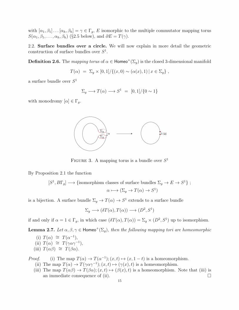
2.2. Surface bundles over a circle. We will now explain in more detail the geometricconstruction of surface bundles over S1.
Definition 2.6. The mapping torus of α ∈ Homeo+(Σg) is the closed 3-dimensional manifold
T (α) = Σg × [0, 1]/(x, 0) ∼ (α(x), 1) |x ∈ Σg ,
a surface bundle over S1
Σg −→ T (α) −→ S1 = [0, 1]/0 ∼ 1
with monodromy [α] ∈ Γg.
T(α : M M)
mapping-torus-2
Σg
Σgα Id
Figure 3. A mapping torus is a bundle over S1
By Proposition 2.1 the function
[S1, BΓg] −→ isomorphism classes of surface bundles Σg → E → S1 ;
α 7−→ (Σg → T (α)→ S1)
is a bijection. A surface bundle Σg → T (α)→ S1 extends to a surface bundle
Σg −→ (δT (α), T (α)) −→ (D2, S1)
if and only if α = 1 ∈ Γg, in which case (δT (α), T (α)) = Σg × (D2, S1) up to isomorphism.
Lemma 2.7. Let α, β, γ ∈ Homeo+(Σg), then the following mapping tori are homeomorphic
(i) T (α) ∼= T (α−1),(ii) T (α) ∼= T (γαγ−1),
(iii) T (αβ) ∼= T (βα).
Proof. (i) The map T (α)→ T (α−1); (x, t) 7→ (x, 1− t) is a homeomorphism.(ii) The map T (α)→ T (γαγ−1); (x, t) 7→ (γ(x), t) is a homeomorphism.
(iii) The map T (αβ) → T (βα); (x, t) 7→ (β(x), t) is a homeomorphism. Note that (iii) isan immediate consequence of (ii).
15
2.3. Surface bundles over a pair of pants. The pair of pants is the oriented surface withboundary defined by the thrice-punctured 2-sphere
(P, ∂P ) = (Σ0,3, ∂Σ0,3)
= (cl.(S2\(D2 tD2 tD2)), S1 t S1 t S1)
with χ(P ) = −1. The pair of pants P is homotopy equivalent to the figure 8, S1 ∨ S1, sothat the three inclusions S1 ⊂ ∂P → P induce morphisms
π1(S1) = Z −→ π1(P ) = Z ∗ Z = 〈x, y〉 ; 11 7−→ x , 12 7−→ y , 13 7−→ xy .
Example 2.8. For any α ∈ Homeo+(Σg) let N1, N2 be the two null-cobordisms of Σg×0, 1defined by
i1 : Σg × 0, 1 −→ N1 = Σg × I ; (x, 0) 7−→ (x, 0) , (x, 1) 7−→ (x, 1) ,
i2 : Σg × 0, 1 −→ N2 = Σg × I ; (x, 0) 7−→ (x, 0) , (x, 1) 7−→ (α(x), 1) .
The twisted double is the mapping torus of α
D(N1, N2, i1, i2) = T (α) .
Definition 2.9. For any α, β ∈ Homeo+(Σg) let N1, N2, N3 be the three null-cobordisms ofΣg × 0, 1 defined by
i1 : Σg × 0, 1 −→ N1 = Σg × I ; (x, 0) 7−→ (x, 0) , (x, 1) 7−→ (x, 1) ,
i2 : Σg × 0, 1 −→ N2 = Σg × I ; (x, 0) 7−→ (x, 0) , (x, 1) 7−→ (α(x), 1) ,
i3 : Σg × 0, 1 −→ N3 = Σg × I ; (x, 0) 7−→ (x, 0) , (x, 1) 7−→ (β(x), 1) .
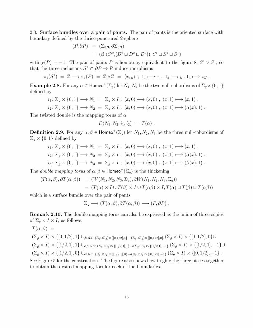
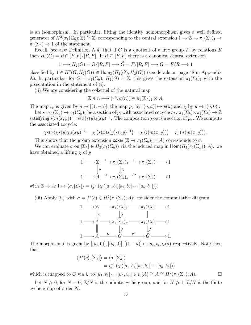
The double mapping torus of α, β ∈ Homeo+(Σg) is the thickening
(T (α, β), ∂T (α, β)) = (W (N1, N2, N3,Σg), ∂W (N1, N2, N3,Σg))
= (T (α)× I ∪ T (β)× I ∪ T (αβ)× I, T (α) t T (β) t T (αβ))
which is a surface bundle over the pair of pants
Σg −→ (T (α, β), ∂T (α, β)) −→ (P, ∂P ) .
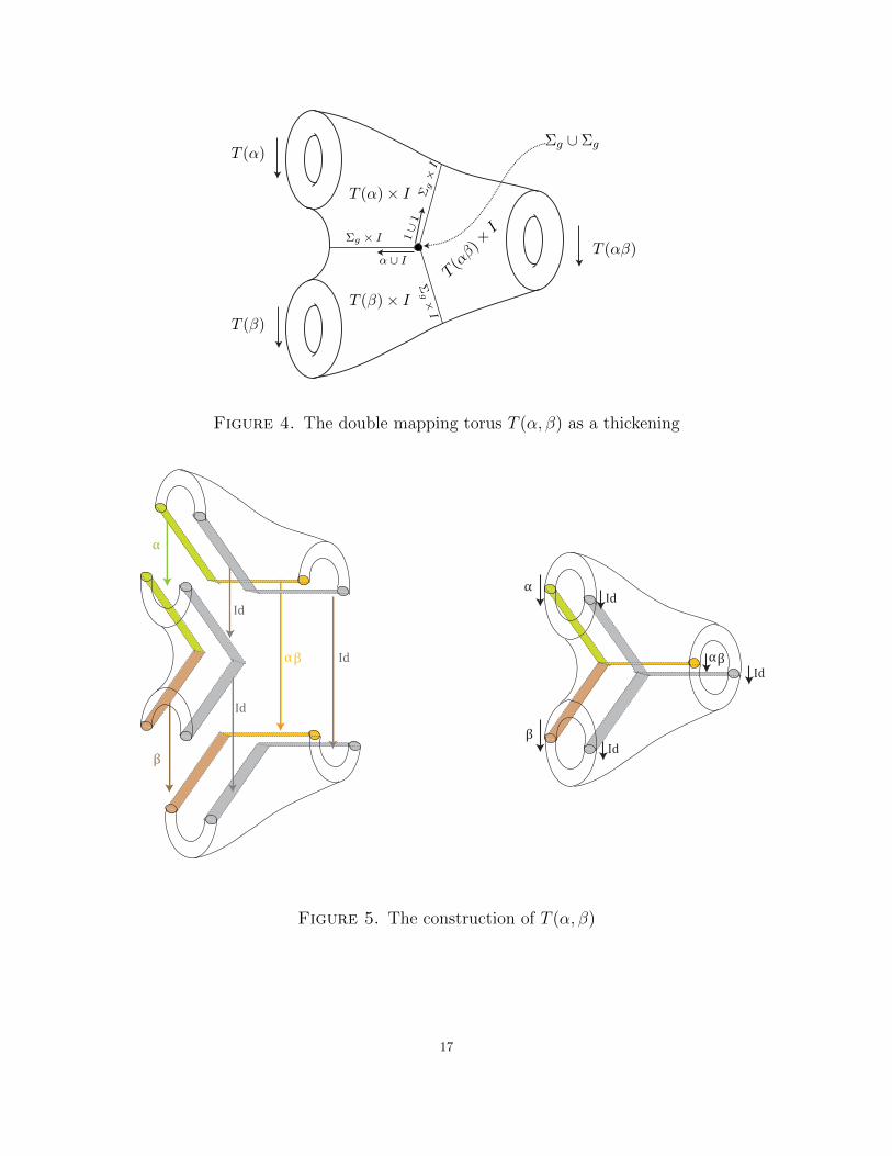
Remark 2.10. The double mapping torus can also be expressed as the union of three copiesof Σg × I × I, as follows:
T (α, β) =
(Σg × I)× [0, 1/2], 1 ∪βtId : (ΣgtΣg)×[0,1/2],1→(ΣgtΣg)×[0,1/2],0 (Σg × I)× [0, 1/2], 0∪(Σg × I)× [1/2, 1], 1 ∪αβtId : (ΣgtΣg)×[1/2,1],1→(ΣgtΣg)×[1/2,1],−1 (Σg × I)× [1/2, 1],−1∪(Σg × I)× [1/2, 1], 0 ∪αtId : (ΣgtΣg)×[1/2,1],0→(ΣgtΣg)×[0,1/2],−1 (Σg × I)× [0, 1/2],−1 .
See Figure 5 for the construction. The figure also shows how to glue the three pieces togetherto obtain the desired mapping tori for each of the boundaries.
16
α
α
α
Id
β
T(β) x I
βdouble-mappingtorus-trisection-simple
N x I1
N x I2
N x I3
T (α)
T (β)
T (αβ)
T (α)× I
T (β)× IT(αβ)×I
Σg×I
Σg×I
Σg × I
α ∪ I
1∪
1
Σg ∪ Σg
Figure 4. The double mapping torus T (α, β) as a thickening
α α
α
α
α
αIdαβ
β
β
β
αβ
β
Id
Id
IdId
Id
Id
double-mappingtorus-blownup
Figure 5. The construction of T (α, β)
17
By Proposition 2.1 the function
[P,BΓg] = [S1 ∨ S1, BΓg]
−→ isomorphism classes of surface bundles Σg → E → P ;
(α, β) 7−→ (Σg → T (α, β)→ P )
is a bijection.
2.4. Surface bundles over a punctured torus. The punctured torus is the 2-dimensionalmanifold with boundary (Q, ∂Q) = (Σ1,1, S
1)
α
α
α
α
α
α
Id
β
β
β
β
Id
Id Id
Id
Id
S(α, β)
S(alpha, beta)
Q
S1
Figure 6. The punctured torus (Q, ∂Q)
with χ(Q) = −1. The punctured torus Q is homotopy equivalent to the figure eight S1∨S1,with the inclusion ∂Q→ Q inducing the morphism
π1(∂Q) = Z −→ π1(Q) = Z ∗ Z = 〈x, y〉 ; 1 7−→ [x, y] .
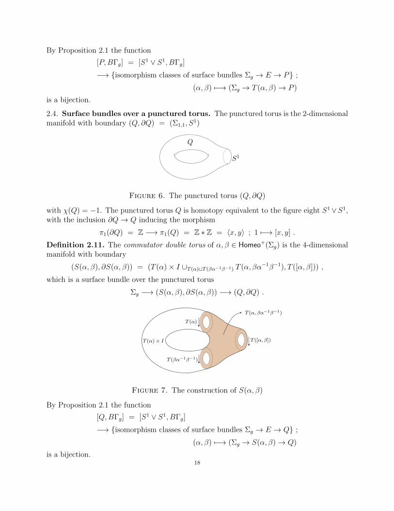
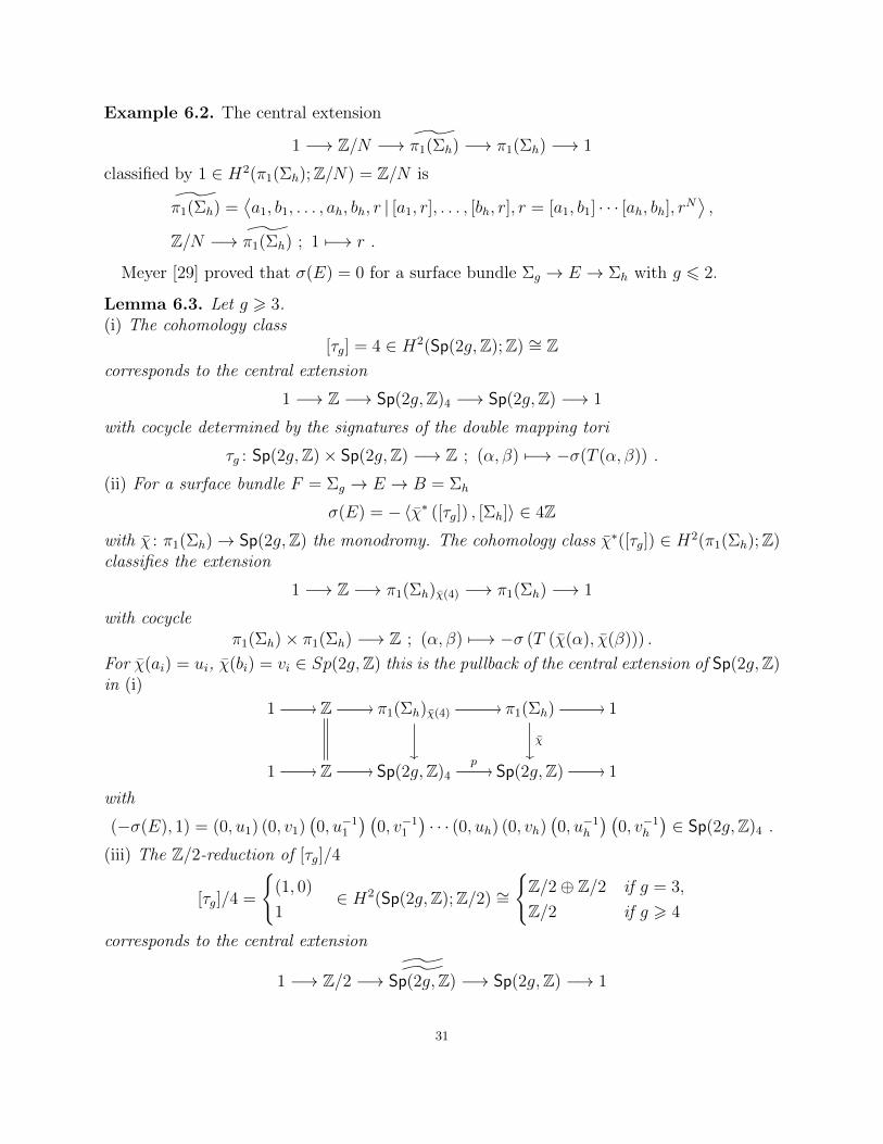
Definition 2.11. The commutator double torus of α, β ∈ Homeo+(Σg) is the 4-dimensionalmanifold with boundary
(S(α, β), ∂S(α, β)) = (T (α)× I ∪T (α)tT (βα−1β−1) T (α, βα−1β−1), T ([α, β])) ,
which is a surface bundle over the punctured torus
Σg −→ (S(α, β), ∂S(α, β)) −→ (Q, ∂Q) .
α
α
α
α
α
α
Id
β
β
β
β
Id
Id Id
Id
Id
α, β β T( )
αα-1 -1
S(α, β)
S(alpha, beta)
T (α)× I
T (α)
T (βα−1β−1)
T ([α, β])
T (α, βα−1β−1)
Figure 7. The construction of S(α, β)
By Proposition 2.1 the function
[Q,BΓg] = [S1 ∨ S1, BΓg]
−→ isomorphism classes of surface bundles Σg → E → Q ;
(α, β) 7−→ (Σg → S(α, β)→ Q)
is a bijection.18
2.5. Surface bundles over a surface. Meyer [28, Satz III. 8.1] used a decomposition ofΣh,k along 3h+ k − 1 Jordan curves to express the signature σ(E) ∈ Z of a surface bundle
Σg −→ E −→ Σh,k
in terms of the monodromy χ : π1(Σh,k)→ Γg. In the special case k = 1 we shall now obtainsuch an expression for σ(E) using 2h− 1 Jordan curves, with Σh,1 a union of h− 1 pairs ofpants and h punctured tori, which gives a more direct relationship between the algebra andthe topology.
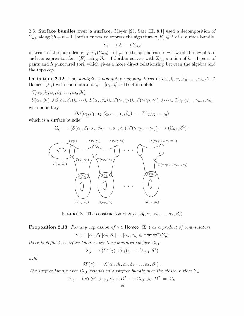
Definition 2.12. The multiple commutator mapping torus of α1, β1, α2, β2, . . . , αh, βh ∈Homeo+(Σg) with commutators γi = [αi, βi] is the 4-manifold
S(α1, β1, α2, β2, . . . , αh, βh) =
S(α1, β1) ∪ S(α2, β2) ∪ · · · ∪ S(αh, βh) ∪ T (γ1, γ2) ∪ T (γ1γ2, γ3) ∪ · · · ∪ T (γ1γ2 . . . γh−1, γh)
with boundary∂S(α1, β1, α2, β2, . . . , αh, βh) = T (γ1γ2 . . . γh)
which is a surface bundle
Σg −→ (S(α1, β1, α2, β2, . . . , αh, βh), T (γ1γ2 . . . γh)) −→ (Σh,1, S1) .
α
α
α
α
α
α
Id
β
β
β
β
α β
β
Id
Id Id
Id
Id
S(x , y )
T([x , y ])
T([α , β ])
S(x , y )
S(α , β )
S(x , y )h h
4 4
3 3
4 4
34
4
1
1
∑ x Dg2
∑ x Sg1
Wee-monster
S(α, β) = T(αβ, β α ) T(αβ) x I-1-1
S(α , β ) S(α , β ) S(α , β ) S(α , β )h h4 43 32 2
S(α1, β1)
S(α2, β2) S(α3, β3) S(αh, βh)
T (γ1, γ2) T (γ1γ2, γ3)
T (γ1γ2 . . . γh−1, γh)
T (γ1) T (γ1γ2) T (γ1γ2γ3) T (γ1γ2 . . . γh = 1)
T (γ2) T (γ3) T (γh)
Figure 8. The construction of S(α1, β1, α2, β2, . . . , αh, βh)
Proposition 2.13. For any expression of γ ∈ Homeo+(Σg) as a product of commutators
γ = [α1, β1][α2, β2] . . . [αh, βh] ∈ Homeo+(Σg)
there is defined a surface bundle over the punctured surface Σh,1
Σg −→ (δT (γ), T (γ)) −→ (Σh,1, S1)
withδT (γ) = S(α1, β1, α2, β2, . . . , αh, βh) .
The surface bundle over Σh,1 extends to a surface bundle over the closed surface Σh
Σg −→ δT (γ) ∪T (γ) Σg ×D2 −→ Σh,1 ∪S1 D2 = Σh
19
if and only if [γ] = 1 ∈ Γg.
α
α
α
α
α
α
Id
β
β
β
β
α β
β
Id
Id Id
Id
Id
S(x , y )
T([x , y ])
T([α , β ])
S(x , y )
S(α , β )
S(x , y )h h
4 4
3 3
4 4
34
4
1
1
∑ x Sg
Wee-monster
S(α, β) = T(αβ, β α ) T(αβ) x I-1-1
S(α , β ) S(α , β ) S(α , β ) S(α , β )h h4 43 32 2
S(α1, β1)
S(α2, β2) S(α3, β3) S(αh, βh)
T (γ1, γ2) T (γ1γ2, γ3)
T (γ1γ2 . . . γh−1, γh)
Σg ×D2
T (γ1) T (γ1γ2) T (γ1γ2γ3)T (γ1γ2 . . . γh = 1)
T (γ2) T (γ3) T (γh)
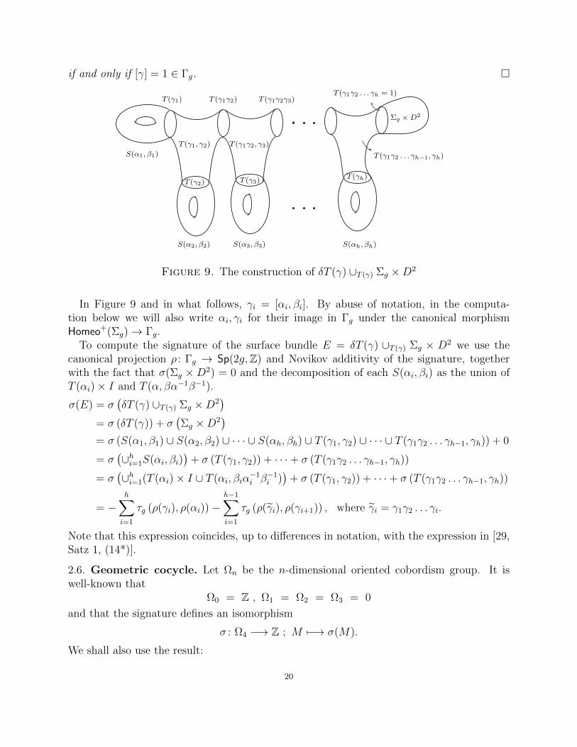
Figure 9. The construction of δT (γ) ∪T (γ) Σg ×D2
In Figure 9 and in what follows, γi = [αi, βi]. By abuse of notation, in the computa-tion below we will also write αi, γi for their image in Γg under the canonical morphismHomeo+(Σg)→ Γg.
To compute the signature of the surface bundle E = δT (γ) ∪T (γ) Σg × D2 we use thecanonical projection ρ : Γg → Sp(2g,Z) and Novikov additivity of the signature, togetherwith the fact that σ(Σg ×D2) = 0 and the decomposition of each S(αi, βi) as the union ofT (αi)× I and T (α, βα−1β−1).
σ(E) = σ(δT (γ) ∪T (γ) Σg ×D2
)= σ (δT (γ)) + σ
(Σg ×D2
)= σ (S(α1, β1) ∪ S(α2, β2) ∪ · · · ∪ S(αh, βh) ∪ T (γ1, γ2) ∪ · · · ∪ T (γ1γ2 . . . γh−1, γh)) + 0
= σ(∪hi=1S(αi, βi)
)+ σ (T (γ1, γ2)) + · · ·+ σ (T (γ1γ2 . . . γh−1, γh))
= σ(∪hi=1(T (αi)× I ∪ T (αi, βiα
−1i β−1
i ))
+ σ (T (γ1, γ2)) + · · ·+ σ (T (γ1γ2 . . . γh−1, γh))
= −h∑i=1
τg (ρ(γi), ρ(αi))−h−1∑i=1
τg (ρ(γi), ρ(γi+1)) , where γi = γ1γ2 . . . γi.
Note that this expression coincides, up to differences in notation, with the expression in [29,Satz 1, (14*)].
2.6. Geometric cocycle. Let Ωn be the n-dimensional oriented cobordism group. It iswell-known that
Ω0 = Z , Ω1 = Ω2 = Ω3 = 0
and that the signature defines an isomorphism
σ : Ω4 −→ Z ; M 7−→ σ(M).
We shall also use the result:
20
Proposition 2.14. [14, Theorem 5.2] For g > 3 the mapping class group Γg is perfect, i.e.every γ ∈ Γg is a product of commutators
γ = [α1, β1][α2, β2] . . . [αh, βh] ∈ Γg .
Proposition 2.15. (i) If Γg is perfect we have a geometric central extension
1 −→ Ω4 −→ Γg −→ Γg −→ 1
with
Γg = (α ∈ Γg, δT (α) = null-cobordism of T (α)) ,
Γg × Γg −→ Γg ; ((α, δT (α)), (β, δT (β))) 7−→ (αβ, T (α, β) ∪ δT (α) ∪ δT (β)) .
(ii) A section Γg → Γg;α 7→ δT (α) determines a cocycle
τ geo : Γg × Γg −→ Ω4 ; (α, β) 7−→ T (α, β) ∪ δT (α) ∪ δT (β) ∪ δT (αβ)
for the class [τ geo] ∈ H2(Γg; Ω4).
Proof. (i) Note that since since Ω3 = 0, and the mapping tori T (α), T (β) and T (αβ) are3-dimensional closed manifolds, then the nullbordims δT (α), δT (β) and δT (αβ) always exist.
(ii) By definition, for G a group and A an abelian group, a cocycle is a function τ : G×G→A such that
τ(x, y) + τ(xy, z) = τ(y, z) + τ(x, yz) ∈ A (x, y, z ∈ G) .
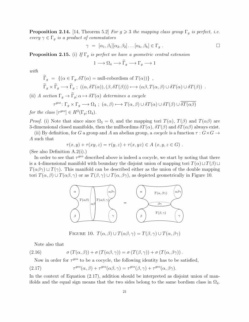
(See also Definition A.2(i).)In order to see that τ geo described above is indeed a cocycle, we start by noting that there
is a 4-dimensional manifold with boundary the disjoint union of mapping tori T (α)tT (β)tT (αβγ) t T (γ). This manifold can be described either as the union of the double mappingtori T (α, β) ∪ T (αβ, γ) or as T (β, γ) ∪ T (α, βγ), as depicted geometrically in Figure 10.
α
α
α
α
α
α
Idα
ββ
β
β
αβ
β
Id
Id
Id
Id
Id
double-mappingtorus-blownup
α
β
αβγ
γ
α
β
αβγ
γ
αβ βγT (αβ) T (αβ, γ)
T (α, βγ)
T (β, γ)
Figure 10. T (α, β) ∪ T (αβ, γ) = T (β, γ) ∪ T (α, βγ)
Note also that
(2.16) σ (T (α, β)) + σ (T (αβ, γ)) = σ (T (β, γ)) + σ (T (α, βγ)) .
Now in order for τ geo to be a cocycle, the following identity has to be satisfied,
(2.17) τ geo(α, β) + τ geo(αβ, γ) = τ geo(β, γ) + τ geo(α, βγ).
In the context of Equation (2.17), addition should be interpreted as disjoint union of man-ifolds and the equal sign means that the two sides belong to the same bordism class in Ω4.
21
Since there is an isomorphism σ : Ω4 → Z, to check that these manifolds belong to the samebordism class we will only need to check that they have the same signature. That is,
σ(T (α, β) ∪ δT (α) ∪ δT (β) ∪ δT (αβ)
)+ σ
(T (αβ, γ) ∪ δT (αβ) ∪ δT (γ) ∪ δT (αβγ)
)= σ
(T (β, γ) ∪ δT (β) ∪ δT (γ) ∪ δT (βγ)
)+ σ
(T (α, βγ) ∪ δT (α) ∪ δT (βγ) ∪ δT (αβγ)
).
Using Novikov additivity of the signature and Equation (2.16), we see that this identityholds, and hence τ geo is a cocycle.
3. Cohomology of Lie groups made discrete
For any discrete group G the group cohomology H2(G;Z) is isomorphic to the degree twocohomology H2(BG;Z) of the classifying space BG. It classifies central group extensions
1 −→ Z −→ G −→ G −→ 1.
A cocycle τ : G×G→ Z determines a central group extension
1 −→ Z −→ Z×τ G −→ G −→ 1
withZ×τ G = (m, a) |m ∈ Z, a ∈ G , (m, a)(n, b) = (m+ n+ τ(a, b), ab) .
A (finite dimensional) Lie group G has a classifying space BG as a topological group. Thesingular cohomology H2(BG;Z) classifies covering groups
1 −→ Z −→ G −→ G −→ 1
where G is again a Lie group.We write Gδ for the same Lie group, but with the discrete topology. Following Milnor
[30] (see also Thurston [38]) we write G for the homotopy fibre of Gδ → G. The goal of thissection is to recap some of what is known about the natural map H2(BG;Z)→ H2(BGδ;Z).
Example 3.1. Let G = R, the additive group of the real numbers. Since G is contractiblewe have G = Gδ.
Now R is a Q-vector space of dimension equal to the cardinality of the continuum. SinceQ is a filtered colimit of rank one free groups, we have H1(BQδ) ∼= Q and Hi(BQδ) = 0 fori > 1. The Kunneth theorem then gives Hi(BRδ) ∼= Λi
Q(R), the ith exterior power of thereals over the rationals. This is a rational vector space of dimension equal to the continuum.By the universal coefficient theorem,
H i(BRδ;Z) ∼= Ext(Λi−1Q (R),Z),
which is again a large rational vector space (note that Ext(Q,Z) is already an uncountabledimensional rational vector space).
Example 3.2. Let G = U(1) ∼= S1. The universal cover of G is R, so we have a pullbacksquare
Rδ //
R
Gδ // G.22
Since R is contractible, this implies that G = Rδ. Thinking of U(1) as a K(Z, 1), we have afibre sequence
K(Z, 1) −→ K(Rδ, 1) −→ K(Gδ, 1) −→ K(Z, 2).
We have H1(BGδ) = R/Z, H1(BRδ) = Rδ. The Gysin sequence of the fibration S1 →K(Rδ, 1)→ K(Gδ, 1) is
· · · −→ H1(BGδ) −→ H2(BRδ) −→ H2(BGδ) −→ H0(BGδ) −→ H1(BRδ) −→ H1(BGδ) −→ 0
and therefore takes the form
· · · −→ R/Z −→ Λ2Q(R) −→ H2(BGδ) −→ Z −→ Rδ −→ Gδ −→ 0.
Since there are no non-trivial homomorphisms from R/Z to a rational vector space, it followsthat
H2(BGδ) ∼= Λ2Q(R).
In cohomology, we have H1(BGδ;Z) = 0 and
H2(BGδ;Z) ∼= Ext(R/Z,Z) ∼= Z⊕ Ext(R,Z),
a direct sum of Z and a large rational vector space.
More generally, it is shown in Sah and Wagoner [34, p. 623] that if G is a simply connectedLie group such that the simply connected composition factors of G are either R or isomorphicto universal covering groups of Chevalley groups over R or C then the integral homologyH2(BGδ) is a Q-vector space of dimension equal to the continuum.
Example 3.3. Let us examine the real Chevalley group Sp(2g,R). In this case, the universalcover is given by
1 −→ Z −→ ˜Sp(2g,R) −→ Sp(2g,R) −→ 1.
Thus
H2(BSp(2g,R)δ;Z) ∼= H2(BSp(2g,R);Z)⊕H2(B ˜Sp(2g,R)δ;Z)
is a direct sum of Z and a Q-vector space of dimension equal to the continuum.
In light of the size of H2(BGδ;Z), we clearly need to restrict the kind of cocycles we shouldconsider, in order to identify the central extensions which are also covering groups; namelythose that are in the image of H2(BG;Z)→ H2(BGδ;Z). It is clearly no use trying to restrictto continuous cocycles; for example if G is connected then the only continuous cocycles arethe constant ones. So what should we try? This problem was solved by Mackey [26], asfollows.
Recall that given a topological space, the Borel sets are the smallest collection of subsetscontaining the open sets, and closed under complementation and arbitrary unions. A map isa Borel map if the inverse image of every Borel set is a Borel set. Theorem 7.1 of Mackey’spaper [26] implies that under reasonably general conditions, given just the Borel sets and agroup structure on G consisting of Borel maps, there is a unique structure of locally compacttopological group on G for which these are the Borel sets and group structure. The proofdepends on Weil’s converse to Haar’s theorem on measures, described in Appendix 1 of Weil[40]. In particular, the topology can be obtained by taking for the neighbourhood system of
23
the identity element in G the family of all sets of the form A−1A, where A is a Borel set ofpositive measure.
The consequence of Mackey’s theorem which we wish to describe is as follows. Given acocycle G×G→ Z which is also a Borel map then consider the covering group
1 −→ Z −→ G −→ G −→ 1.
The group G inherits a Borel structure, as the underlying set is G× Z. This is compatiblewith the group structure, and so by Mackey’s theorem G is a topological group in a uniqueway. Uniqueness of the structure of topological group on G implies that the topologicalgroup G/Z is isomorphic to G, and therefore the map G→ G is continuous. It follows thatG is a Lie group.
Definition 3.4. The Borel cohomology H2B(G;Z) is the abelian group of Borel cocycles on
Gδ modulo coboundaries of Borel cochains Gδ → Z.
Milnor [30, Theorem 1] proved that for any Lie group G with finitely many connectedcomponents the natural map H2(BG;Z)→ H2(BGδ;Z) is injective.
Theorem 3.5. For any Lie group G with finitely many connected components, the image ofthe injection H2(BG;Z)→ H2(BGδ;Z) is equal to the image of H2
B(G;Z)→ H2(Gδ;Z).
Proof. By the commutativity of the diagram
H2(BG;Z) //
∼=
H2(BGδ;Z)
∼=
H2B(G;Z) // H2(Gδ;Z).
This can be found in [9, below Theorem 2.1]. It follows from work of Wigner [41], and canbe best understood by combining [31, Theorem 10] (see also [10, Theorem 38]), and [2, p.1518].
4. Cocycles on S1δ
We are concerned in this section with certain Borel cocycles τ : S1δ × S1δ → Z on the(discrete) circle group S1δ, and the covering groups they define. We shall think of S1δ as theunit interval [0, 1] with the endpoints identified, using the group isomorphism
[0, 1]/(0 ∼ 1)∼=// S1δ ; a 7−→ e2πia
as an identification.The “standard cocycle” is given by
τ : [0, 1)× [0, 1) −→ Z ; (a, b) 7−→ τ(a, b) =
0 if 0 6 a+ b < 1,
1 if 1 6 a+ b < 2.
This defines the extension
1 −→ Z −→ Rδ −→ S1δ −→ 1.
24
We shall say that a cochain f is nice if it is piecewise constant. In other words, S1 is dividedinto a finite number of intervals with open or closed ends, on each of which f is constant.We shall say that a coboundary τ is nice if it is the coboundary of a nice cochain, and weshall say that a cocycle is nice if it is the sum of a nice coboundary and an integer multiplem of the standard cocycle. Every nice cocycle defines a topological covering group of S1,and by Theorem 3.5 and Proposition 5.2 below, the quotient of the nice cocycles by the nicecoboundaries gives H2
B(S1;Z) ∼= Z, with generator the class [τ ] of the standard cocycle. Theinteger m, which we call the covering number of the cocycle τ , is thus well defined. If m = 0then the covering is trivial:
1 −→ Z −→ S1δ × Z −→ S1δ −→ 1,
while if m 6= 0, the covering takes the form
1 −→ Z −→ Rδ ×mτ Zm −→ S1δ −→ 1.
(See Definition A.2 for background on group extensions.)We can draw a picture of a nice cocycle τ in an obvious way, by dividing [0, 1]× [0, 1] into
subregions where τ is constant.
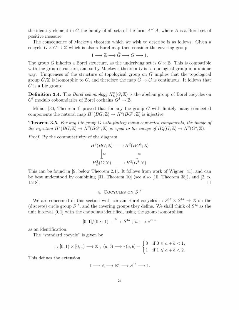
Example 4.1. The standard cocycle gives the following picture:
@@@
@@@
0
1
This is a Borel cocycle on S1δ because it is piecewise constant on Borel subsets.
Theorem 4.2. The picture of a nice cocycle has only horizontal, vertical and leading diagonalboundary lines. The covering number can be computed by looking at the diagonal lines only.For each diagonal line segment, we compute ((value of cocycle above the line segment) minus(value of cocycle below the line segment)) × length of line segment, normalised so that thenumber of segments in the main diagonal is equal to one. Adding these quantities gives thecovering number.
Proof. The quantity described in the theorem is additive on nice cocycles, so we only need tocheck the theorem on the standard cocycle and on coboundaries. For the standard cocycle,there is just one diagonal line segment, and the difference in the values from below to abovethe line segment is one, so the theorem is true in this case. For a nice coboundary δf , thediagonal lines happen where f(a + b) changes in value. For each point in the unit intervalwhere f changes value, the total normalised length of the one or two diagonal line segmentsrepresenting the change in value of f(a + b) is equal to one. So we are adding the changesin value of f as f goes once round S1. The total is therefore zero.
Notice that in this theorem, the values of τ on the boundaries of regions are irrelevant tothe computation of the covering number.
25
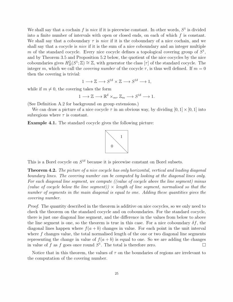
Example 4.3. For any p, q ∈ Z define the nice cochain
f(p, q) : [0, 1) −→ Z ; a 7−→
p if 0 6 a < 1/2,
q if 1/2 6 a < 1
with nice coboundary
δf(p, q) : [0, 1)× [0, 1) −→ Z ; (a, b) 7−→ f(a) + f(b)− f(a+ b) .
For any m ∈ Z the picture of the nice cocycle m(standard) + δf(p, q) has 8 regions
p
2p− q
p
m+ q
p
m+ q
m− p+ 2q
m+ q
with covering number
1
2((2p− q)− p) + (m+ q − p) +
1
2((m+ q)− (m− p+ 2q)) = m .
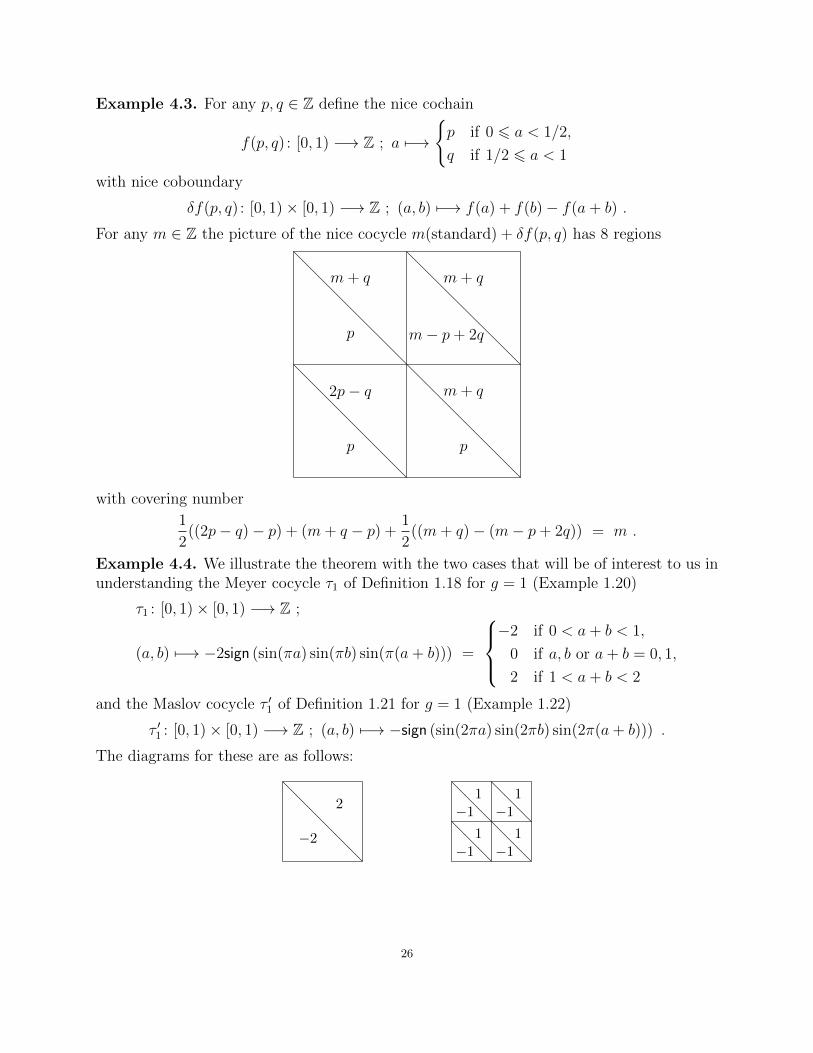
Example 4.4. We illustrate the theorem with the two cases that will be of interest to us inunderstanding the Meyer cocycle τ1 of Definition 1.18 for g = 1 (Example 1.20)
τ1 : [0, 1)× [0, 1) −→ Z ;
(a, b) 7−→ −2sign (sin(πa) sin(πb) sin(π(a+ b))) =
−2 if 0 < a+ b < 1,
0 if a, b or a+ b = 0, 1,
2 if 1 < a+ b < 2
and the Maslov cocycle τ ′1 of Definition 1.21 for g = 1 (Example 1.22)
τ ′1 : [0, 1)× [0, 1) −→ Z ; (a, b) 7−→ −sign (sin(2πa) sin(2πb) sin(2π(a+ b))) .
The diagrams for these are as follows:
@@@@@@
−2
2
@@@
@@@
@@@
@@@
−11
−11
−11
−11
26
In the terminology of Example 4.3
τ1 = 4(standard) + δf(−2,−2) ,
τ ′1 = 4(standard) + δf(−1,−3) ,
so that the covering number is equal to 4 in both cases. Now
f(1,−1)(a) = sign(sin 2πa) ,
so that the cocycles differ by the coboundary
τ1(a, b)− τ ′1(a, b) = −δf(1,−1)(a, b)
= −sign(sin 2πa)− sign(sin 2πb) + sign(sin 2π(a+ b)) .
and[τ1] = [τ ′1] = 4 ∈ H2
b (S1;Z) = Z .
(See also Example 1.22 and Remark 1.23.)
5. The symplectic group Sp(2g,R)
In this section, we examine the homotopy type and cohomology of Sp(2g,R), and use thisto compare the cocycles described in Sections 1 and 4.
Theorem 5.1. Let G be a Lie group with finitely many connected components, and let K bea maximal compact subgroup. Then as a topological space, G is homeomorphic to a Cartesianproduct K ×Rd, where d is the codimension of K in G. In particular, the inclusion of K inG is a homotopy equivalence.
Proof. See Theorem 3.1 in Chapter XV of Hochschild [19].
In the case of Sp(2g,R), a connected Lie group of dimension g(2g + 1), the maximalcompact subgroup is the unitary group U(g) of dimension g2. Thus as a topological space,we have Sp(2g,R) ∼= U(g)× Rg(g+1).
Proposition 5.2. The inclusion U(g) → Sp(2g,R) of topological groups is a homotopyequivalence. Thus we have π1(Sp(2g,R)) ∼= Z and
H∗(BSp(2g,R);Z) ∼= Z[c1, . . . , cg],
where ci ∈ H2i(BSp(2g,R);Z) = H2i(BU(g);Z) denotes the i-th Chern class.
Proof. This follows from Theorem 5.1 and well known properties of U(g).
As π1(Sp(2g,R)) ∼= Z, the universal cover is a group ˜Sp(2g,R) sitting in a central extension
1 −→ Z −→ ˜Sp(2g,R) −→ Sp(2g,R) −→ 1.
Provided g > 4, pulling back the universal cover of Sp(2g,R) to the perfect group Sp(2g,Z)gives the universal central extension
1 −→ Z −→ ˜Sp(2g,Z) −→ Sp(2g,Z) −→ 1.
For more about this group, see Section 7.2.
27
Corollary 5.3. The coset space Sp(2g,R)/Sp(2g − 2,R) is homeomorphic to a Cartesianproduct S2g−1 × R2g.
Corollary 5.4. The inclusions
S1 = U(1) −→ Sp(2,R) −→ Sp(4,R) −→ · · · −→ Sp(2g,R)
induce isomorphisms on π1.
Proof. By the long homotopy exact sequence of a fibration.
Corollary 5.5. The Borel cohomology H2B(Sp(2g,R);Z) is isomorphic to Z, with generator
c1. The restriction map
H2B(Sp(2g,R);Z) −→ H2
B(Sp(2g − 2,R);Z)
is an isomorphism.
Proof. Proposition 5.2 contains the information that H2B(Sp(2g,R);Z) ∼= Z. The claim on
the restriction map follows from the Serre spectral sequence of a fibration and the fact thatSp(2g,R)/Sp(2g − 2,R) is (2g − 2)-connected for g ≥ 2.
Theorem 5.6. The cohomology class in H2B(Sp(2g,R);Z) ∼= H2(BSp(2g,R);Z) ∼= Z defined
by the Meyer cocycle τg and the Maslov cocycle τ ′g are both equal to 4c1.
Proof. Remember from Theorem 3.5 that H2B(Sp(2g,R);Z) ∼= H2(BSp(2g,R);Z), which is
Z by Corollary 5.5, and that it injects into H2(Sp(2g,R)δ;Z). It follows from Proposition1.24 and Corollaries 5.4, 5.5 that it suffices to prove the second statement for the subgroupS1 = U(1) ⊆ Sp(2,R). In this case, the Meyer cocycle is represented by the first diagram inExample 4.4, while the Maslov cocycle is represented by the second diagram. According toTheorem 4.2, these both have covering number 4. The standard cocycle on S1δ is Borel andhas covering number 1 (see beginning of Section 4). By Corollary 5.5 it is thus the restrictionto S1δ of a cocycle on Sp(2,R) representing c1.
6. The signature of a surface bundle modulo eight
Let Σg → E → Σh be a surface bundle, with fibre the surface Σg of genus g > 1, and basethe surface Σh of genus h > 1. We shall use the Z/4-coefficient monodromy
π1(Σh) −→ Γg −→ Sp(2g,Z) −→ Sp(2g,Z/4)
to provide a recipe for computing the signature of the 4-manifold E modulo eight.We start with some generalities about central group extensions and commutators.For any abelian group A there is defined a cap product pairing
H2(Σh;A)×H2(Σh) −→ H0(Σh;A) = A ; (σ, [Σh]) 7−→ 〈σ, [Σh]〉with [Σh] ∈ H2(Σh) the fundamental class. In the first instance, we obtain a formula for〈σ, [Σh]〉 ∈ A in terms of the central extension
1 −→ A −→ π1(Σh)σ −→ π1(Σh) −→ 1
classified by σ ∈ H2(Σh;A) = H2(π1(Σh);A). The fundamental group of Σh is the onerelator group given by
π1(Σh) = 〈a1, b1, a2, b2, . . . , ah, bh | r〉28
where r = [a1, b1][a2, b2] · · · [ah, bh] is the single relator.
Lemma 6.1. (i) The central extension classified by 1 ∈ H2(π1(Σh);Z) ∼= Z
1 −→ Z i−→ π1(Σh)1p−→ π1(Σh) −→ 1
is given by
π1(Σh)1 = 〈a1, b1, . . . , ah, bh, r | [a1, r], . . . , [bh, r], r = [a1, b1] · · · [ah, bh]〉 ,i : Z −→ π1(Σh)1 ; 1 7−→ r .
(ii) Let 1→ A→ π1(Σh)σ → π1(Σh)→ 1 be the central extension classified by an element
σ ∈ H2(Σh;A) ∼= H2(π1(Σh);A) ∼= Hom(H2(π1(Σh)), A) ∼= A .
Thenπ1(Σh)σ = coker (Z −→ π1(Σh)1 × A)
fits into a morphism of central extensions
1 // Z i//
σ
π1(Σh)1p//
χ
π1(Σh) // 1
1 // Aiσ// π1(Σh)σ
pσ// π1(Σh) // 1
such that〈σ, [Σh]〉 = χ ([a1, b1][a2, b2] · · · [ah, bh]) ∈ A ⊂ π1(Σh)σ .
(iii) For any group G, abelian group A and cohomology class c ∈ H2(G;A) let
1 −→ A −→ Gp−→ G −→ 1
be the central extension of G by A classified by c. A group morphism f : π1(Σh) → G isdetermined by elements u1, v1, . . . , uh, vh ∈ G such that [u1, v1] · · · [uh, vh] ∈ A, with f(ai) =p(ui), f(bi) = p(vi). The pullback central extension H of π1(Σh) by A
1 // A // H //
f
π1(Σh) //
f
1
1 // Aic// G
pc// G // 1
is classified byf ∗(c) = [u1, v1] · · · [uh, vh] ∈ H2(π1(Σh);A) ∼= A
so that H = π1(Σh)f∗(c).
Proof. (i) This can be seen by construction. We propose also a more general method thatwill be useful in the rest of the proof.
Since h > 1, Σh is a K(π1(Σh), 1), so that
H1(π1(Σh)) = H1(Σh) = Z2h , H2(π1(Σh)) = H2(Σh) = Z .
In particular,Ext1Z(H1(π1(Σh)), H2(π1(Σh))) = 0,
and so the universal coefficient sequence shows that
H2(π1(Σh);H2(π1(Σh))) −→ HomZ(H2(π1(Σh)), H2(π1(Σh)))
29
is an isomorphism. In particular, lifting the identity homomorphism gives a well definedgenerator of H2(π1(Σh);Z) ∼= Z, corresponding to the central extension 1→ Z→ π1(Σh)1 →π1(Σh)→ 1 of the statement.
Recall (see also Definition A.4) that if G is a quotient of a free group F by relations Rthen H2(G) = R ∩ [F, F ]/[R,F ]. If R ⊆ [F, F ] there is a canonical central extension
1 −→ H2(G) = R/[R,F ] −→ G = F/[R,F ] −→ G = F/R −→ 1
classified by 1 ∈ H2(G;H2(G)) ∼= HomZ(H2(G), H2(G)) (see details on page 48 in AppendixA). In particular, for G = π1(Σh), H2(G) = Z, this gives the extension π1(Σh)1 with thepresentation in the statement of (i).
(ii) We are considering the cokernel of the natural map
Z 3 n 7−→ (rn, σ(n)) ∈ π1(Σh)1 × A.The map iσ is given by a 7→ [(1,−a)], the map pσ by [(u, a)] 7→ p(u) and χ by u 7→ [(u, 0)].
Let s : π1(Σh)→ π1(Σh)1 be a section of p, with associated cocyclem : π1(Σh)×π1(Σh)→ Zsatisfying i(m(x, y)) = s(x)s(y)s(xy)−1. The composition χs is a section of pσ. We computethe associated cocycle:
χs(x)χs(y)χs(xy)−1 = χ(s(x)s(y)s(xy)−1
)= χ (i(m(x, y))) = iσ (σ(m(x, y))) .
This shows that the group extension coker (Z→ π1(Σh)1 × A) corresponds to σ.We can evaluate σ on [Σh] ∈ H2(π1(Σh)) via the induced map in Hom(H2(π1(Σh)), A): we
have obtained a lifting χ of p
1 // Z i//
σ
π1(Σh)1p//
χ
π1(Σh) // 1
1 // Aiσ// π1(Σh)σ
pσ// π1(Σh) // 1
with Z→ A; 1 7→ 〈σ, [Σh]〉 = i−1σ (χ ([a1, b1][a2, b2] · · · [ah, bh])).
(iii) Apply (ii) with σ = f ∗(c) ∈ H2(π1(Σh);A): consider the commutative diagram
1 // Z //
σ
π1(Σh)1//
χ
π1(Σh) // 1
1 // A // π1(Σh)σ //
f
π1(Σh) //
f
1
1 // Aic// G
pc// G // 1.
The morphism f is given by [(ai, 0)], [(bi, 0)], [(1,−a)] 7→ ui, vi, ic(a) respectively. Note thenthat ⟨
f ∗(c), [Σh]⟩
= 〈σ, [Σh]〉= i−1
σ (χ ([a1, b1][a2, b2] · · · [ah, bh]))which is mapped to G via ic to [u1, v1] · · · [uh, vh] ∈ ic(A) ∼= A ∼= H2(π1(Σh);A).
Let N > 0; for N = 0, Z/N is the infinite cyclic group, and for N > 1, Z/N is the finitecyclic group of order N .
30
Example 6.2. The central extension
1 −→ Z/N −→ π1(Σh) −→ π1(Σh) −→ 1
classified by 1 ∈ H2(π1(Σh);Z/N) = Z/N is
π1(Σh) =⟨a1, b1, . . . , ah, bh, r | [a1, r], . . . , [bh, r], r = [a1, b1] · · · [ah, bh], rN
⟩,
Z/N −→ π1(Σh) ; 1 7−→ r .
Meyer [29] proved that σ(E) = 0 for a surface bundle Σg → E → Σh with g 6 2.
Lemma 6.3. Let g > 3.(i) The cohomology class
[τg] = 4 ∈ H2(Sp(2g,Z);Z) ∼= Zcorresponds to the central extension
1 −→ Z −→ Sp(2g,Z)4 −→ Sp(2g,Z) −→ 1
with cocycle determined by the signatures of the double mapping tori
τg : Sp(2g,Z)× Sp(2g,Z) −→ Z ; (α, β) 7−→ −σ(T (α, β)) .
(ii) For a surface bundle F = Σg → E → B = Σh
σ(E) = −〈χ∗ ([τg]) , [Σh]〉 ∈ 4Zwith χ : π1(Σh)→ Sp(2g,Z) the monodromy. The cohomology class χ∗([τg]) ∈ H2(π1(Σh);Z)classifies the extension
1 −→ Z −→ π1(Σh)χ(4) −→ π1(Σh) −→ 1
with cocycleπ1(Σh)× π1(Σh) −→ Z ; (α, β) 7−→ −σ (T (χ(α), χ(β))) .
For χ(ai) = ui, χ(bi) = vi ∈ Sp(2g,Z) this is the pullback of the central extension of Sp(2g,Z)in (i)
1 // Z // π1(Σh)χ(4)//
π1(Σh)
χ
// 1
1 // Z // Sp(2g,Z)4p// Sp(2g,Z) // 1
with
(−σ(E), 1) = (0, u1) (0, v1)(0, u−1
1
) (0, v−1
1
)· · · (0, uh) (0, vh)
(0, u−1
h
) (0, v−1
h
)∈ Sp(2g,Z)4 .
(iii) The Z/2-reduction of [τg]/4
[τg]/4 =
(1, 0)
1∈ H2(Sp(2g,Z);Z/2) ∼=
Z/2⊕ Z/2 if g = 3,
Z/2 if g > 4
corresponds to the central extension
1 −→ Z/2 −→˜
Sp(2g,Z) −→ Sp(2g,Z) −→ 1
31
such that for a surface bundle Σg →M → Σh
σ(E)/4 = 〈χ∗ ([τg]/4) , [Σh]〉 ∈ Z/2 .
Proof. (i)+(ii) Meyer [29].(iii) From (i) we have that [τg]/4 = 1 ∈ H2(Sp(2g,Z);Z) ∼= Z is the generator of thiscohomology group. By naturality of the universal coefficient theorem and because the groupSp(2g,Z) is perfect for g ≥ 3, one has a commutative diagram
H2(Sp(2g,Z);Z)r2
//
∼=
H2(Sp(2g,Z);Z/2)
∼=
Hom(H2(Sp(2g,Z);Z),Z)r2// Hom(H2(Sp(2g,Z);Z),Z/2).
Lemma B.1(iii), (v) and (vi) gives
H2(Sp(2g,Z);Z) =
Z⊕ Z/2 if g = 3,
Z if g ≥ 4,
H2(Sp(2g,Z);Z) = Z if g ≥ 3, and
H2(Sp(2g,Z);Z/2) =
Z/2⊕ Z/2 if g = 3,
Z/2 if g ≥ 4.
Consulting Lemma B.1(x), the map r2 has imageZ/2⊕ 0 if g = 3,
Z/2 if g ≥ 4
and r2([τg]/4) is (1, 0) if g = 3,
1 if g ≥ 4.
7. Signature of surface bundles modulo an integer
7.1. Signatures of surface bundles mod N for N 6 8. In [5] we showed the existenceof a cohomology class in the second cohomology group of a finite quotient H of Sp(2g,Z)that computes the mod 2 reduction of signature/4 for a surface bundle over a surface.
We recall this theorem in detail hereafter. It chases the cohomology class from the finitegroup H = Sp(2g,Z)/K to Meyer’s class on Sp(2g,Z). We include details of low genus cases,which makes the theorem a little hard to follow, so afterwards we summarise the situationin a diagram valid for g > 4.
As in [5] we write Γ(2g,N) E Sp(2g,Z) for the principal congruence subgroup consistingof symplectic matrices which are congruent to the identity modulo N .
Definition 7.1. For g > 1 we write K (resp. Y) for the subgroup of Sp(2g,Z) (resp.Sp(2g,Z/4)) consisting of matrices(
I + 2a 2b2c I + 2d
)∈ Sp(2g,Z) (resp. Sp(2g,Z/4))
32
satisfying:
(i) The vectors of diagonal entries Diag(b) and Diag(c) are even, and(ii) the trace Tr(a) is even (equivalently, Tr(d) is even).
Theorem 7.2. Let g ≥ 2.
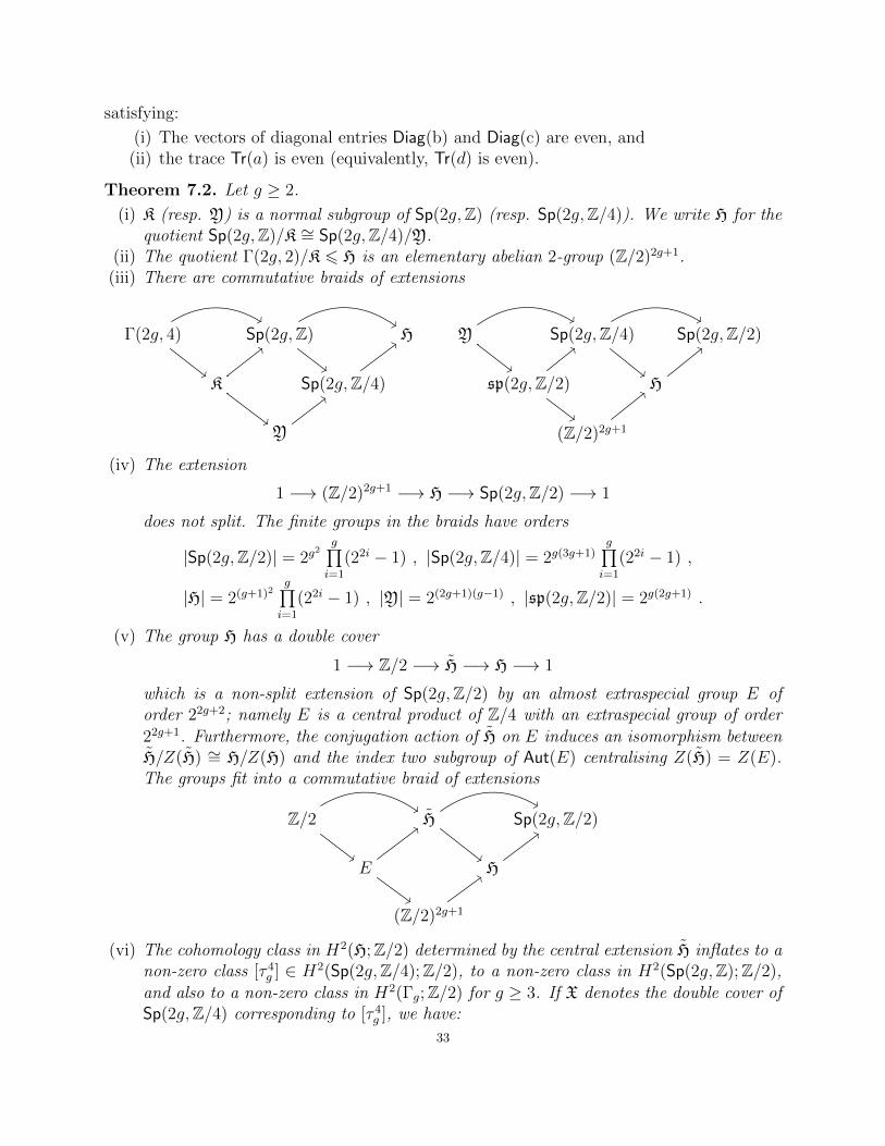
(i) K (resp. Y) is a normal subgroup of Sp(2g,Z) (resp. Sp(2g,Z/4)). We write H for thequotient Sp(2g,Z)/K ∼= Sp(2g,Z/4)/Y.
(ii) The quotient Γ(2g, 2)/K 6 H is an elementary abelian 2-group (Z/2)2g+1.(iii) There are commutative braids of extensions
Γ(2g, 4)
##
%%
Sp(2g,Z)
##
$$
H
K
;;
##
Sp(2g,Z/4)
;;
Y
;;
Y
##
%%
Sp(2g,Z/4)
##
%%
Sp(2g,Z/2)
sp(2g,Z/2)
;;
""
H
;;
(Z/2)2g+1
<<
(iv) The extension
1 −→ (Z/2)2g+1 −→ H −→ Sp(2g,Z/2) −→ 1
does not split. The finite groups in the braids have orders
|Sp(2g,Z/2)| = 2g2
g∏i=1
(22i − 1) , |Sp(2g,Z/4)| = 2g(3g+1)g∏i=1
(22i − 1) ,
|H| = 2(g+1)2g∏i=1
(22i − 1) , |Y| = 2(2g+1)(g−1) , |sp(2g,Z/2)| = 2g(2g+1) .
(v) The group H has a double cover
1 −→ Z/2 −→ H −→ H −→ 1
which is a non-split extension of Sp(2g,Z/2) by an almost extraspecial group E oforder 22g+2; namely E is a central product of Z/4 with an extraspecial group of order
22g+1. Furthermore, the conjugation action of H on E induces an isomorphism betweenH/Z(H) ∼= H/Z(H) and the index two subgroup of Aut(E) centralising Z(H) = Z(E).The groups fit into a commutative braid of extensions
Z/2
##
$$
H
##
%%
Sp(2g,Z/2)
E
;;
##
H
;;
(Z/2)2g+1
;;
(vi) The cohomology class in H2(H;Z/2) determined by the central extension H inflates to anon-zero class [τ 4
g ] ∈ H2(Sp(2g,Z/4);Z/2), to a non-zero class in H2(Sp(2g,Z);Z/2),
and also to a non-zero class in H2(Γg;Z/2) for g ≥ 3. If X denotes the double cover ofSp(2g,Z/4) corresponding to [τ 4
g ], we have:
33
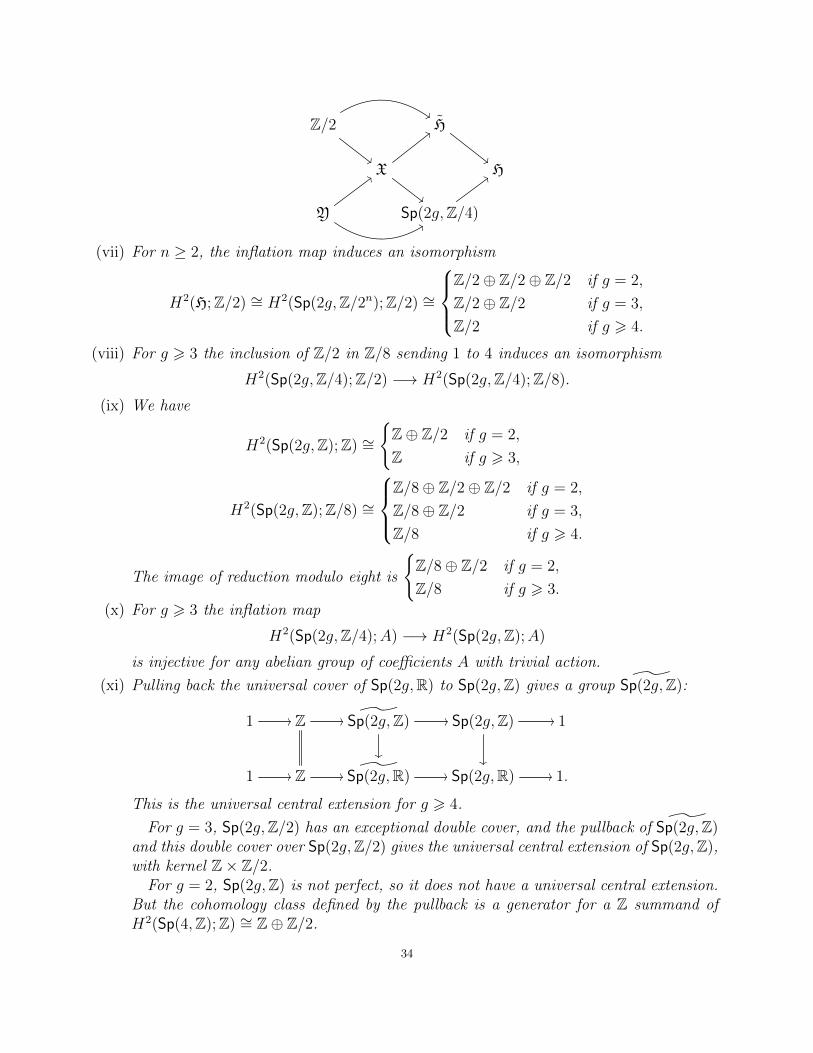
Z/2
##
$$
H
##
X
;;
##
H
Y
;;
99Sp(2g,Z/4)
;;
(vii) For n ≥ 2, the inflation map induces an isomorphism
H2(H;Z/2) ∼= H2(Sp(2g,Z/2n);Z/2) ∼=
Z/2⊕ Z/2⊕ Z/2 if g = 2,
Z/2⊕ Z/2 if g = 3,
Z/2 if g > 4.
(viii) For g > 3 the inclusion of Z/2 in Z/8 sending 1 to 4 induces an isomorphism
H2(Sp(2g,Z/4);Z/2) −→ H2(Sp(2g,Z/4);Z/8).
(ix) We have
H2(Sp(2g,Z);Z) ∼=
Z⊕ Z/2 if g = 2,
Z if g > 3,
H2(Sp(2g,Z);Z/8) ∼=
Z/8⊕ Z/2⊕ Z/2 if g = 2,
Z/8⊕ Z/2 if g = 3,
Z/8 if g > 4.
The image of reduction modulo eight is
Z/8⊕ Z/2 if g = 2,
Z/8 if g > 3.
(x) For g > 3 the inflation map
H2(Sp(2g,Z/4);A) −→ H2(Sp(2g,Z);A)
is injective for any abelian group of coefficients A with trivial action.
(xi) Pulling back the universal cover of Sp(2g,R) to Sp(2g,Z) gives a group ˜Sp(2g,Z):
1 // Z // ˜Sp(2g,Z) //
Sp(2g,Z) //
1
1 // Z // ˜Sp(2g,R) // Sp(2g,R) // 1.
This is the universal central extension for g > 4.
For g = 3, Sp(2g,Z/2) has an exceptional double cover, and the pullback of ˜Sp(2g,Z)and this double cover over Sp(2g,Z/2) gives the universal central extension of Sp(2g,Z),with kernel Z× Z/2.
For g = 2, Sp(2g,Z) is not perfect, so it does not have a universal central extension.But the cohomology class defined by the pullback is a generator for a Z summand ofH2(Sp(4,Z);Z) ∼= Z⊕ Z/2.
34
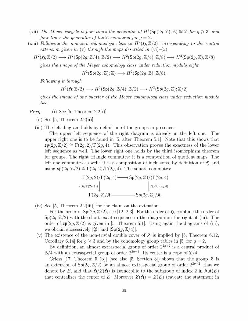
(xii) The Meyer cocycle is four times the generator of H2(Sp(2g,Z);Z) ∼= Z for g > 3, andfour times the generator of the Z summand for g = 2.
(xiii) Following the non-zero cohomology class in H2(H;Z/2) corresponding to the centralextension given in (v) through the maps described in (vi)–(x)
H2(H;Z/2) −→ H2(Sp(2g,Z/4);Z/2) −→ H2(Sp(2g,Z/4);Z/8) −→ H2(Sp(2g,Z);Z/8)
gives the image of the Meyer cohomology class under reduction modulo eight
H2(Sp(2g,Z);Z) −→ H2(Sp(2g,Z);Z/8).
Following it through
H2(H;Z/2) −→ H2(Sp(2g,Z/4);Z/2) −→ H2(Sp(2g,Z);Z/2)
gives the image of one quarter of the Meyer cohomology class under reduction modulotwo.
Proof. (i) See [5, Theorem 2.2(i)].
(ii) See [5, Theorem 2.2(ii)].
(iii) The left diagram holds by definition of the groups in presence.The upper left sequence of the right diagram is already in the left one. The
upper right one is to be found in [5, after Theorem 5.1]. Note that this shows thatsp(2g,Z/2) ∼= Γ(2g, 2)/Γ(2g, 4). This observation proves the exactness of the lowerleft sequence as well. The lower right one holds by the third isomorphism theoremfor groups. The right triangle commutes: it is a composition of quotient maps. Theleft one commutes as well: it is a composition of inclusions, by definition of Y andusing sp(2g,Z/2) ∼= Γ(2g, 2)/Γ(2g, 4). The square commutes:
Γ(2g, 2)/Γ(2g, 4)
//
/(K/Γ(2g,4))
Sp(2g,Z)/(Γ(2g, 4)
/(K/Γ(2g,4))
Γ(2g, 2)/K
// Sp(2g,Z)/K.
(iv) See [5, Theorem 2.2(iii)] for the claim on the extension.For the order of Sp(2g,Z/2), see [12, 2.3]. For the order of H, combine the order of
Sp(2g,Z/2) with the short exact sequence in the diagram on the right of (iii). Theorder of sp(2g,Z/2) is given in [5, Theorem 5.1]. Using again the diagrams of (iii),we obtain successively |Y| and |Sp(2g,Z/4)|.
(v) The existence of the non-trivial double cover of H is implied by [5, Theorem 6.12,Corollary 6.14] for g ≥ 3 and by the cohomology group tables in [5] for g = 2.
By definition, an almost extraspecial group of order 22g+2 is a central product ofZ/4 with an extraspecial group of order 22g+1. Its center is a copy of Z/4.
Griess [17, Theorem 5 (b)] (see also [5, Section 3]) shows that the group H isan extension of Sp(2g,Z/2) by an almost extraspecial group of order 22g+2, that we
denote by E, and that H/Z(H) is isomorphic to the subgroup of index 2 in Aut(E)
that centralizes the center of E. Moreover Z(H) = Z(E) (caveat: the statement in
35
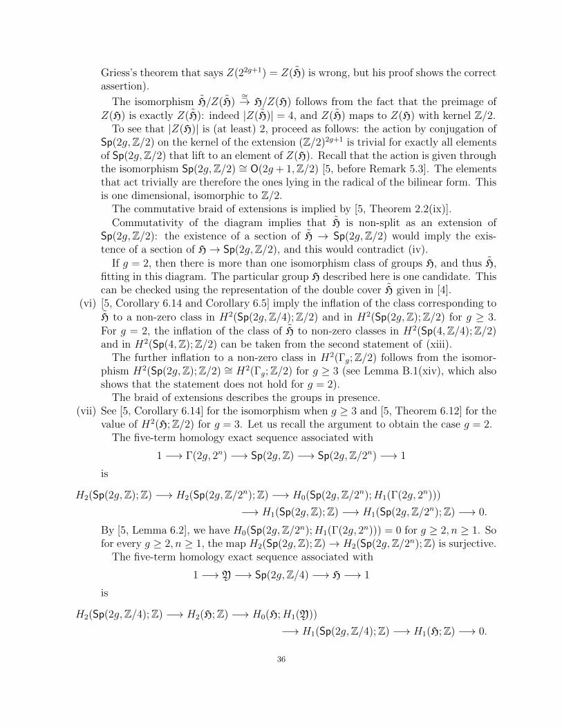
Griess’s theorem that says Z(22g+1) = Z(H) is wrong, but his proof shows the correctassertion).
The isomorphism H/Z(H)∼=→ H/Z(H) follows from the fact that the preimage of
Z(H) is exactly Z(H): indeed |Z(H)| = 4, and Z(H) maps to Z(H) with kernel Z/2.To see that |Z(H)| is (at least) 2, proceed as follows: the action by conjugation of
Sp(2g,Z/2) on the kernel of the extension (Z/2)2g+1 is trivial for exactly all elementsof Sp(2g,Z/2) that lift to an element of Z(H). Recall that the action is given throughthe isomorphism Sp(2g,Z/2) ∼= O(2g + 1,Z/2) [5, before Remark 5.3]. The elementsthat act trivially are therefore the ones lying in the radical of the bilinear form. Thisis one dimensional, isomorphic to Z/2.
The commutative braid of extensions is implied by [5, Theorem 2.2(ix)].
Commutativity of the diagram implies that H is non-split as an extension ofSp(2g,Z/2): the existence of a section of H → Sp(2g,Z/2) would imply the exis-tence of a section of H→ Sp(2g,Z/2), and this would contradict (iv).
If g = 2, then there is more than one isomorphism class of groups H, and thus H,fitting in this diagram. The particular group H described here is one candidate. Thiscan be checked using the representation of the double cover H given in [4].
(vi) [5, Corollary 6.14 and Corollary 6.5] imply the inflation of the class corresponding to
H to a non-zero class in H2(Sp(2g,Z/4);Z/2) and in H2(Sp(2g,Z);Z/2) for g ≥ 3.
For g = 2, the inflation of the class of H to non-zero classes in H2(Sp(4,Z/4);Z/2)and in H2(Sp(4,Z);Z/2) can be taken from the second statement of (xiii).
The further inflation to a non-zero class in H2(Γg;Z/2) follows from the isomor-phism H2(Sp(2g,Z);Z/2) ∼= H2(Γg;Z/2) for g ≥ 3 (see Lemma B.1(xiv), which alsoshows that the statement does not hold for g = 2).
The braid of extensions describes the groups in presence.(vii) See [5, Corollary 6.14] for the isomorphism when g ≥ 3 and [5, Theorem 6.12] for the
value of H2(H;Z/2) for g = 3. Let us recall the argument to obtain the case g = 2.The five-term homology exact sequence associated with
1 −→ Γ(2g, 2n) −→ Sp(2g,Z) −→ Sp(2g,Z/2n) −→ 1
is
H2(Sp(2g,Z);Z) −→ H2(Sp(2g,Z/2n);Z) −→ H0(Sp(2g,Z/2n);H1(Γ(2g, 2n)))
−→ H1(Sp(2g,Z);Z) −→ H1(Sp(2g,Z/2n);Z) −→ 0.
By [5, Lemma 6.2], we have H0(Sp(2g,Z/2n);H1(Γ(2g, 2n))) = 0 for g ≥ 2, n ≥ 1. Sofor every g ≥ 2, n ≥ 1, the map H2(Sp(2g,Z);Z)→ H2(Sp(2g,Z/2n);Z) is surjective.
The five-term homology exact sequence associated with
1 −→ Y −→ Sp(2g,Z/4) −→ H −→ 1
is
H2(Sp(2g,Z/4);Z) −→ H2(H;Z) −→ H0(H;H1(Y))
−→ H1(Sp(2g,Z/4);Z) −→ H1(H;Z) −→ 0.
36
By [5, Lemma 5.5(i) and proof of Proposition 6.6] we have H0(H;H1(Y)) = 0 forg ≥ 1. The map H2(Sp(2g,Z/4);Z)→ H2(H;Z) is thus surjective for g ≥ 1. Togetherwith the above this implies that H2(Sp(2g,Z/2n);Z)→ H2(H;Z) is surjective for allg, n ≥ 2. Consider the sequence of induced maps
Hom(H2(Sp(2g,Z);Z),Z/2)←− Hom(H2(Sp(2g,Z/2n);Z),Z/2)←− Hom(H2(H;Z),Z/2).
By the above both are injective for g, n ≥ 2. Insert the values of H2(Sp(2g,Z);Z)(Lemma B.1(iii)) and H2(H;Z) [5, Tables]. We see that both maps must be isomor-phisms for g, n ≥ 2. By the universal coefficient theorem this finishes the proof forg ≥ 3, as each of Sp(2g,Z), Sp(2g,Z/2n), and H are perfect.
For g = 2, we need to also consider the Ext-terms coming from H1(Sp(2g,Z);Z),H1(Sp(2g,Z/2n);Z), and H1(H;Z). By the five-term exact sequences above, themaps H1(Sp(2g,Z);Z)→ H1(Sp(2g,Z/2n) for every n ≥ 1 and H1(Sp(2g,Z/4);Z)→H1(H;Z) are surjective. This implies that
H1(Sp(2g,Z/2n) −→ H1(H;Z)
is surjective for all n ≥ 2 as well. Insert the values of H1(Sp(2g,Z);Z) (LemmaB.1(ii)) and H1(H;Z) [5, Tables]. The composition
Z/2 ∼= H1(Sp(2g,Z);Z) −→ H1(Sp(2g,Z/2n);Z) −→ H1(H;Z) ∼= Z/2is surjective, thus also injective. Then each of the two maps is an isomorphism, andthus by functoriality we obtain isomorphisms also for
Ext1Z(H1(H;Z),Z/2) −→ Ext1Z(H1(Sp(2g,Z/2n);Z),Z/2) −→ Ext1Z(H1(Sp(2g,Z);Z),Z/2)
for every n ≥ 2. This together with the preceding results on the Hom-term finishesthe proof for g = 2.
(viii) (See also [8, Chapter 6].) We consider the following short exact sequence:
0 // Z/2 i// Z/8
p// Z/4 // 0,
where i is the map sending 1 to 4. The induced long exact sequence in cohomologyfor Sp(2g,Z/4) is:
... H1(Sp(2g,Z/4);Z/4)
H2(Sp(2g,Z/4);Z/2) H2(Sp(2g,Z/4);Z/8) H2(Sp(2g,Z/4);Z/4)
H3(Sp(2g,Z/4);Z/2) ...
p∗
∂1
i∗ p∗
∂2
i∗
Let g ≥ 3. Then H1(Sp(2g,Z/4);Z/4) = 0 by perfection of the group. Usingthe cohomology computations of Point (vii) and Lemma B.1(ix), we thus have anisomorphism i∗
H2(Sp(2g,Z/4);Z/2)∼=−→ H2(Sp(2g,Z/4);Z/8).37
(ix) See Lemma B.1(v),(vii),(xi).
(x) By [5, Corollary 6.5].
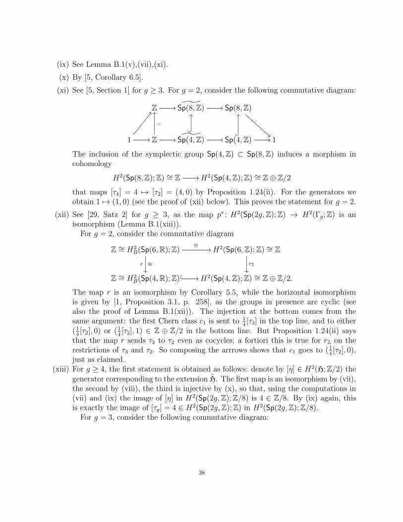
(xi) See [5, Section 1] for g ≥ 3. For g = 2, consider the following commutative diagram:
Z // ˜Sp(8,Z) // Sp(8,Z)
!!
1
BB
// Z //
=
OO
˜Sp(4,Z) //
?
OO
Sp(4,Z)?
OO
// 1
The inclusion of the symplectic group Sp(4,Z) ⊂ Sp(8,Z) induces a morphism incohomology
H2(Sp(8,Z);Z) ∼= Z // H2(Sp(4,Z);Z) ∼= Z⊕ Z/2
that maps [τ4] = 4 7→ [τ2] = (4, 0) by Proposition 1.24(ii). For the generators weobtain 1 7→ (1, 0) (see the proof of (xii) below). This proves the statement for g = 2.
(xii) See [29, Satz 2] for g ≥ 3, as the map p∗ : H2(Sp(2g,Z);Z) → H2(Γg;Z) is anisomorphism (Lemma B.1(xiii)).
For g = 2, consider the commutative diagram
Z ∼= H2B(Sp(6,R);Z)
∼=//
∼=r
H2(Sp(6,Z);Z) ∼= ZrZ
Z ∼= H2B(Sp(4,R);Z)
// H2(Sp(4,Z);Z) ∼= Z⊕ Z/2.
The map r is an isomorphism by Corollary 5.5, while the horizontal isomorphismis given by [1, Proposition 3.1, p. 258], as the groups in presence are cyclic (seealso the proof of Lemma B.1(xii)). The injection at the bottom comes from thesame argument: the first Chern class c1 is sent to 1
4[τ3] in the top line, and to either
(14[τ2], 0) or (1
4[τ2], 1) ∈ Z ⊕ Z/2 in the bottom line. But Proposition 1.24(ii) says
that the map r sends τ3 to τ2 even as cocycles; a fortiori this is true for rZ on therestrictions of τ3 and τ2. So composing the arrrows shows that c1 goes to (1
4[τ2], 0),
just as claimed.(xiii) For g ≥ 4, the first statement is obtained as follows: denote by [η] ∈ H2(H;Z/2) the
generator corresponding to the extension H. The first map is an isomorphism by (vii),the second by (viii), the third is injective by (x), so that, using the computations in(vii) and (ix) the image of [η] in H2(Sp(2g,Z);Z/8) is 4 ∈ Z/8. By (ix) again, thisis exactly the image of [τg] = 4 ∈ H2(Sp(2g,Z);Z) in H2(Sp(2g,Z);Z/8).
For g = 3, consider the following commutative diagram:
38
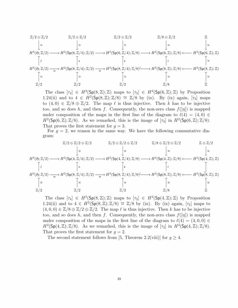
Z/2⊕ Z/2
∼=
Z/2⊕ Z/2
∼=
Z/2⊕ Z/2
∼=
Z/8⊕ Z/2
∼=
Z
∼=
H2(H;Z/2) // H2(Sp(6,Z/4);Z/2) // H2(Sp(6,Z/4);Z/8) // H2(Sp(6,Z);Z/8) H2(Sp(6,Z);Z)oo
H2(H;Z/2) ∼=//
f
OO
H2(Sp(8,Z/4);Z/2) ∼=//
h
OO
H2(Sp(8,Z/4);Z/8)
//
k
OO
H2(Sp(8,Z);Z/8)
`
OO
H2(Sp(8,Z);Z)oo
∼=
OO
Z/2
∼=
OO
Z/2
∼=
OO
Z/2
∼=
OO
Z/8
∼=
OO
Z
∼=
OO
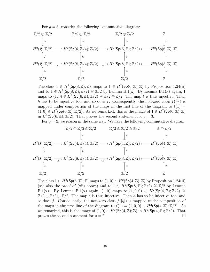
The class [τ4] ∈ H2(Sp(8,Z);Z) maps to [τ3] ∈ H2(Sp(6,Z);Z) by Proposition1.24(ii) and to 4 ∈ H2(Sp(8,Z);Z/8) ∼= Z/8 by (ix). By (ix) again, [τ3] mapsto (4, 0) ∈ Z/8 ⊕ Z/2. The map ` is thus injective. Then k has to be injectivetoo, and so does h, and then f . Consequently, the non-zero class f([η]) is mappedunder composition of the maps in the first line of the diagram to `(4) = (4, 0) ∈H2(Sp(6,Z);Z/8). As we remarked, this is the image of [τ3] in H2(Sp(6,Z);Z/8).That proves the first statement for g = 3.
For g = 2, we reason in the same way. We have the following commutative dia-gram:
Z/2⊕ Z/2⊕ Z/2
∼=
Z/2⊕ Z/2⊕ Z/2
∼=
Z/8⊕ Z/2⊕ Z/2
∼=
Z⊕ Z/2
∼=
H2(H;Z/2) // H2(Sp(4,Z/4);Z/2) // H2(Sp(4,Z/4);Z/8) // H2(Sp(4,Z);Z/8) H2(Sp(4,Z);Z)oo
H2(H;Z/2) ∼=//
f
OO
H2(Sp(8,Z/4);Z/2) ∼=//
h
OO
H2(Sp(8,Z/4);Z/8)
//
k
OO
H2(Sp(8,Z);Z/8)
`
OO
H2(Sp(8,Z);Z)oo?
OO
Z/2
∼=
OO
Z/2
∼=
OO
Z/2
∼=
OO
Z/8
∼=
OO
Z
∼=
OO
The class [τ4] ∈ H2(Sp(8,Z);Z) maps to [τ2] ∈ H2(Sp(4,Z);Z) by Proposition1.24(ii) and to 4 ∈ H2(Sp(8,Z);Z/8) ∼= Z/8 by (ix). By (ix) again, [τ2] maps to(4, 0, 0) ∈ Z/8⊕ Z/2⊕ Z/2. The map ` is thus injective. Then k has to be injectivetoo, and so does h, and then f . Consequently, the non-zero class f([η]) is mappedunder composition of the maps in the first line of the diagram to `(4) = (4, 0, 0) ∈H2(Sp(4,Z);Z/8). As we remarked, this is the image of [τ2] in H2(Sp(4,Z);Z/8).That proves the first statement for g = 2.
The second statement follows from [5, Theorem 2.2(viii)] for g ≥ 4.
39
For g = 3, consider the following commutative diagram:
Z/2⊕ Z/2∼=
Z/2⊕ Z/2∼=
Z/2⊕ Z/2∼=
Z∼=
H2(H;Z/2) // H2(Sp(6,Z/4);Z/2) // H2(Sp(6,Z);Z/2) H2(Sp(6,Z);Z)oo
H2(H;Z/2) ∼=//
f
OO
H2(Sp(8,Z/4);Z/2) ∼=//
h
OO
H2(Sp(8,Z);Z/2)
`
OO
H2(Sp(8,Z);Z)oo
∼=
OO
Z/2
∼=
OO
Z/2
∼=
OO
Z/2
∼=
OO
Z
∼=
OO
The class 1 ∈ H2(Sp(8,Z);Z) maps to 1 ∈ H2(Sp(6,Z);Z) by Proposition 1.24(ii)and to 1 ∈ H2(Sp(8,Z);Z/2) ∼= Z/2 by Lemma B.1(x). By Lemma B.1(x) again, 1maps to (1, 0) ∈ H2(Sp(6,Z);Z/2) ∼= Z/2⊕ Z/2. The map ` is thus injective. Thenh has to be injective too, and so does f . Consequently, the non-zero class f([η]) ismapped under composition of the maps in the first line of the diagram to `(1) =(1, 0) ∈ H2(Sp(6,Z);Z/2). As we remarked, this is the image of 1 ∈ H2(Sp(6,Z);Z)in H2(Sp(6,Z);Z/2). That proves the second statement for g = 3.
For g = 2, we reason in the same way. We have the following commutative diagram:
Z/2⊕ Z/2⊕ Z/2∼=
Z/2⊕ Z/2⊕ Z/2∼=
Z⊕ Z/2∼=
H2(H;Z/2) // H2(Sp(4,Z/4);Z/2) // H2(Sp(4,Z);Z/2) H2(Sp(4,Z);Z)oo
H2(H;Z/2) ∼=//
f
OO
H2(Sp(8,Z/4);Z/2) ∼=//
h
OO
H2(Sp(8,Z);Z/2)
`
OO
H2(Sp(8,Z);Z)oo?
OO
Z/2
∼=
OO
Z/2
∼=
OO
Z/2
∼=
OO
Z
∼=
OO
The class 1 ∈ H2(Sp(8,Z);Z) maps to (1, 0) ∈ H2(Sp(4,Z);Z) by Proposition 1.24(ii)(see also the proof of (xii) above) and to 1 ∈ H2(Sp(8,Z);Z/2) ∼= Z/2 by LemmaB.1(x). By Lemma B.1(x) again, (1, 0) maps to (1, 0, 0) ∈ H2(Sp(4,Z);Z/2) ∼=Z/2 ⊕ Z/2 ⊕ Z/2. The map ` is thus injective. Then h has to be injective too, andso does f . Consequently, the non-zero class f([η]) is mapped under composition ofthe maps in the first line of the diagram to `(1) = (1, 0, 0) ∈ H2(Sp(4,Z);Z/2). Aswe remarked, this is the image of (1, 0) ∈ H2(Sp(4,Z);Z) in H2(Sp(4,Z);Z/2). Thatproves the second statement for g = 2.
40
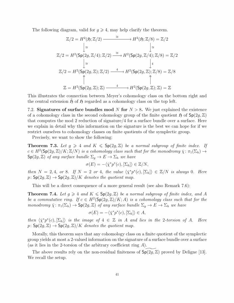
The following diagram, valid for g > 4, may help clarify the theorem.
Z/2 = H2(H;Z/2)∼=
//
∼=
H2(H;Z/8) = Z/2∼=
Z/2 = H2(Sp(2g,Z/4);Z/2)∼=//
∼=
H2(Sp(2g,Z/4);Z/8) = Z/2
4
Z/2 = H2(Sp(2g,Z);Z/2)4// H2(Sp(2g,Z);Z/8) = Z/8
Z = H2(Sp(2g,Z);Z)4
//
OOOO
H2(Sp(2g,Z);Z) = Z
OOOO
This illustrates the connection between Meyer’s cohomology class on the bottom right andthe central extension H of H regarded as a cohomology class on the top left.
7.2. Signatures of surface bundles mod N for N > 8. We just explained the existenceof a cohomology class in the second cohomology group of the finite quotient H of Sp(2g,Z)that computes the mod 2 reduction of signature/4 for a surface bundle over a surface. Herewe explain in detail why this information on the signature is the best we can hope for if werestrict ourselves to cohomology classes on finite quotients of the symplectic group.
Precisely, we want to show the following:
Theorem 7.3. Let g > 4 and K 6 Sp(2g,Z) be a normal subgroup of finite index. Ifc ∈ H2(Sp(2g,Z)/K;Z/N) is a cohomology class such that for the monodromy χ : π1(Σh)→Sp(2g,Z) of any surface bundle Σg → E → Σh we have
σ(E) = −〈χ∗p∗(c), [Σh]〉 ∈ Z/N,then N = 2, 4, or 8. If N = 2 or 4, the value 〈χ∗p∗(c), [Σh]〉 ∈ Z/N is always 0. Herep : Sp(2g,Z)→ Sp(2g,Z)/K denotes the quotient map.
This will be a direct consequence of a more general result (see also Remark 7.6):
Theorem 7.4. Let g > 4 and K 6 Sp(2g,Z) be a normal subgroup of finite index, and Abe a commutative ring. If c ∈ H2(Sp(2g,Z)/K;A) is a cohomology class such that for themonodromy χ : π1(Σh)→ Sp(2g,Z) of any surface bundle Σg → E → Σh we have
σ(E) = −〈χ∗p∗(c), [Σh]〉 ∈ A,then 〈χ∗p∗(c), [Σh]〉 is the image of 4 ∈ Z in A and lies in the 2-torsion of A. Herep : Sp(2g,Z)→ Sp(2g,Z)/K denotes the quotient map.
Morally, this theorem says that any cohomology class on a finite quotient of the symplecticgroup yields at most a 2-valued information on the signature of a surface bundle over a surface(as it lies in the 2-torsion of the arbitrary coefficient ring A).
The above results rely on the non-residual finiteness of ˜Sp(2g,Z) proved by Deligne [13].We recall the setup.
41
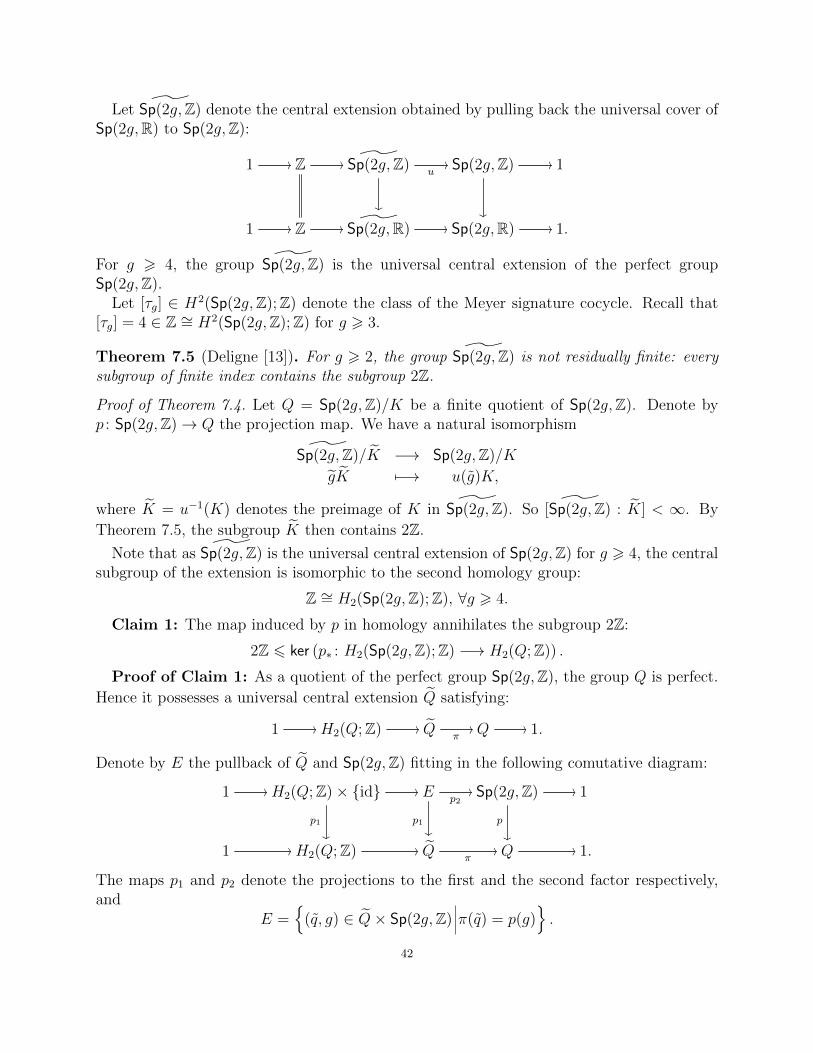
Let ˜Sp(2g,Z) denote the central extension obtained by pulling back the universal cover ofSp(2g,R) to Sp(2g,Z):
1 // Z // ˜Sp(2g,Z)u//
Sp(2g,Z) //
1
1 // Z // ˜Sp(2g,R) // Sp(2g,R) // 1.
For g > 4, the group ˜Sp(2g,Z) is the universal central extension of the perfect groupSp(2g,Z).
Let [τg] ∈ H2(Sp(2g,Z);Z) denote the class of the Meyer signature cocycle. Recall that[τg] = 4 ∈ Z ∼= H2(Sp(2g,Z);Z) for g > 3.
Theorem 7.5 (Deligne [13]). For g > 2, the group ˜Sp(2g,Z) is not residually finite: everysubgroup of finite index contains the subgroup 2Z.
Proof of Theorem 7.4. Let Q = Sp(2g,Z)/K be a finite quotient of Sp(2g,Z). Denote byp : Sp(2g,Z)→ Q the projection map. We have a natural isomorphism
˜Sp(2g,Z)/K −→ Sp(2g,Z)/K
gK 7−→ u(g)K,
where K = u−1(K) denotes the preimage of K in ˜Sp(2g,Z). So [ ˜Sp(2g,Z) : K] < ∞. By
Theorem 7.5, the subgroup K then contains 2Z.
Note that as ˜Sp(2g,Z) is the universal central extension of Sp(2g,Z) for g > 4, the centralsubgroup of the extension is isomorphic to the second homology group:
Z ∼= H2(Sp(2g,Z);Z), ∀g > 4.
Claim 1: The map induced by p in homology annihilates the subgroup 2Z:
2Z 6 ker (p∗ : H2(Sp(2g,Z);Z) −→ H2(Q;Z)) .
Proof of Claim 1: As a quotient of the perfect group Sp(2g,Z), the group Q is perfect.
Hence it possesses a universal central extension Q satisfying:
1 // H2(Q;Z) // Qπ// Q // 1.
Denote by E the pullback of Q and Sp(2g,Z) fitting in the following comutative diagram:
1 // H2(Q;Z)× id //
p1
E
p1
p2// Sp(2g,Z) //
p
1
1 // H2(Q;Z) // Qπ
// Q // 1.
The maps p1 and p2 denote the projections to the first and the second factor respectively,and
E =
(q, g) ∈ Q× Sp(2g,Z) π(q) = p(g).
42
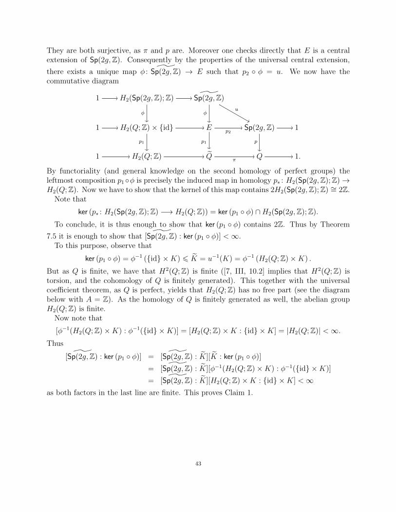
They are both surjective, as π and p are. Moreover one checks directly that E is a centralextension of Sp(2g,Z). Consequently by the properties of the universal central extension,
there exists a unique map φ : ˜Sp(2g,Z) → E such that p2 φ = u. We now have thecommutative diagram
1 // H2(Sp(2g,Z);Z) //
φ
˜Sp(2g,Z)
φ
u
&&
1 // H2(Q;Z)× id //
p1
E
p1
p2// Sp(2g,Z) //
p
1
1 // H2(Q;Z) // Qπ
// Q // 1.
By functoriality (and general knowledge on the second homology of perfect groups) theleftmost composition p1 φ is precisely the induced map in homology p∗ : H2(Sp(2g,Z);Z)→H2(Q;Z). Now we have to show that the kernel of this map contains 2H2(Sp(2g,Z);Z) ∼= 2Z.
Note that
ker (p∗ : H2(Sp(2g,Z);Z) −→ H2(Q;Z)) = ker (p1 φ) ∩H2(Sp(2g,Z);Z).
To conclude, it is thus enough to show that ker (p1 φ) contains 2Z. Thus by Theorem
7.5 it is enough to show that [ ˜Sp(2g,Z) : ker (p1 φ)] <∞.To this purpose, observe that
ker (p1 φ) = φ−1 (id ×K) 6 K = u−1(K) = φ−1 (H2(Q;Z)×K) .
But as Q is finite, we have that H2(Q;Z) is finite ([7, III, 10.2] implies that H2(Q;Z) istorsion, and the cohomology of Q is finitely generated). This together with the universalcoefficient theorem, as Q is perfect, yields that H2(Q;Z) has no free part (see the diagrambelow with A = Z). As the homology of Q is finitely generated as well, the abelian groupH2(Q;Z) is finite.
Now note that
[φ−1(H2(Q;Z)×K) : φ−1(id ×K)] = [H2(Q;Z)×K : id ×K] = |H2(Q;Z)| <∞.Thus
[ ˜Sp(2g,Z) : ker (p1 φ)] = [ ˜Sp(2g,Z) : K][K : ker (p1 φ)]
= [ ˜Sp(2g,Z) : K][φ−1(H2(Q;Z)×K) : φ−1(id ×K)]
= [ ˜Sp(2g,Z) : K][H2(Q;Z)×K : id ×K] <∞as both factors in the last line are finite. This proves Claim 1.
43
As Sp(2g,Z) and Q are perfect, the universal coefficient theorem for cohomology providesthe following commutative diagram:
Hom(H2(Q;Z), A)Hom(p∗)
//
∼=
Hom(H2(Sp(2g,Z);Z), A)
∼=
H2(Q;A)p∗
// H2(Sp(2g,Z);A)
for any principal ideal domain A.Claim 2: Im(p∗) ⊂ T2(H2(Sp(2g,Z);A)), where T2 denotes the 2-torsion.Proof of Claim 2: As indicated by the commutative diagram, the map p∗ is defined as
follows:
H2(Q;A) ∼= Hom(H2(Q;Z), A) 3 α 7−→ αp∗ ∈ Hom(H2(Sp(2g,Z);Z), A) ∼= H2(Sp(2g,Z);A).
Then let g > 4 and n ∈ H2(Sp(2g,Z);Z) ∼= Z. If 2 | n, Claim 1 implies p∗(n) = 0. SoHom(p∗)(α) is determined by Hom(p∗)(α)(1), and we have
2Hom(p∗)(α)(1) = Hom(p∗)(α)(2) = 0.
This proves Claim 2.Note that H2(Sp(2g,Z);A) ∼= Hom(H2(Sp(2g,Z);Z), A) ∼= Hom(Z, A) ∼= A if g > 4.Now comes the final part of the proof. Let [τg]A denote the image of [τg] inH2(Sp(2g,Z);A).
Suppose that there exists a class c ∈ H2(Q;A) such that
p∗(c) = [τg]A.
By Claim 2 we have 2p∗(c) = 0. On the other hand, [τg]A is the image of [τg] = 4 ∈ Z ∼=H2(Sp(2g,Z);Z) in A. So we have
p∗(c) = 4A ∈ T2(A).
Hence this class c can provide at most the 2-valued information 4A on the signature: eitherit is 0 in A or not.
Remark 7.6. In particular, setting A = Z/N , we find the following: 4N ∈ T2(Z/N), and
T2(Z/N) =
0 if N is odd,
0, N2
if N is even.
Hence no information is obtained in this way for odd N . For even N , suppose N2
= 4N .Then
N
2= 4 (mod N)(7.7)
N | N2− 4(7.8)
N
2− 4 = qN for some q ∈ Z(7.9)
N(1− 2q) = 8(7.10)
1− 2q is odd and divides 8(7.11)
44
1− 2q = 1(7.12)
q = 0.(7.13)
So N = 8.
Remark 7.14. If g = 3, the conclusions of Theorems 7.3 and 7.4 still hold, with the sameproof, as the only difference between g = 3 and g > 4 is an additional 2-torsion summand inthe second homology of the symplectic group with integer coefficients (Lemma B.1(iii)) aswell as a 2-torsion factor in the universal extension of Sp(6,Z) (Theorem 7.2(xi)).
Appendix A. Homology and cohomology of groups
Let G be a discrete group, and A a Z[G]-module.The homology Hn(G;A) and cohomology groups Hn(G;A) (n > 0) are the abelian groups
defined in terms of homological algebra by
Hn(G;A) = TorZ[G]n (Z, A) = Hn(P ⊗Z[G] A) ,
Hn(G;A) = ExtnZ[G](Z, A) = Hn(HomZ[G](P,A))
with P a projective Z[G]-module resolution of Z with the trivial Z[G]-action. In terms ofthe classifying space BG
Hn(G;A) = Hn(BG;A) , Hn(G;A) = Hn(BG;A) (n > 0) .
We shall only be concerned with the case when A is an abelian group with the trivialZ[G]-action. The homology and cohomology groups are related by the universal coefficienttheorem exact sequence
0 −→ Ext1Z(Hn−1(G;Z), A) −→ Hn(G;A) −→ HomZ(Hn(G;Z), A) −→ 0 .
For A = Z writeHn(G;Z) = Hn(G) , Hn(G;Z) = Hn(G)
as usual. We shall only be concerned with the cases n = 1, 2, when the homology andcohomology groups have more direct expressions in terms of group theory.
Definition A.1. Let G be a group.(i) The commutator of x, y ∈ G is the element
[x, y] = xyx−1y−1 ∈ G .
For any subsets X, Y ⊆ G let [X, Y ] / G be the normal subgroup generated by the commu-tators [x, y] ∈ G (x ∈ X, y ∈ Y ).(ii) The first homology group of G is the abelian group
H1(G) = Gab = G/[G,G] .
The group G is perfect if H1(G) = 0, or equivalently G = [G,G].(iii) The first cohomology group of G is the abelian group
H1(G) = HomZ(H1(G),Z) .
(iv) For any abelian group A,
H1(G;A) = H1(G)⊗ A , H1(G;A) = HomZ(H1(G), A) .
45
For any space X and any abelian group A there are defined isomorphisms
H1(X;A) −→ HomZ(H1(X), A) ; f 7−→ (x 7−→ f(x)) ,
[X,BA] −→ H1(X;A) ; (f : X −→ BA) 7−→ (f∗ : π1(X) −→ A) .
It follows that for the classifying space X = BG of a discrete group G the function
H1(G;A) −→ H1(BG;A) = [BG,BA] ; f 7−→ Bf
is an isomorphism.
Definition A.2. Let G be a group, and A an abelian group.(i) A cocycle is a function τ : G×G→ A such that
τ(x, y) + τ(xy, z) = τ(y, z) + τ(x, yz) ∈ A (x, y, z ∈ G) .
(ii) A cocycle τ determines a central extension
1 −→ A −→ A×τ G −→ G −→ 1
with the group structure on A×τ G = A×G given by
(A×τ G)× (A×τ G) −→ A×τ G; ((a, x), (b, y)) 7−→ (a+ b+ τ(x, y), xy) .
(iii) A cochain is a function f : G→ A, with coboundary the cocycle
δf : G×G −→ A; (x, y) 7−→ δf(x, y) = f(x) + f(y)− f(xy) .
(iv) The second cohomology group H2(G,A) is the abelian group of equivalence classes [τ ]of cocycles τ : G×G −→ A with
τ ∼ τ ′ if τ − τ ′ = δf for some cochain f : G→ A .
The addition is by the addition of cocycles.
Definition A.3. (i) An extension of a group G by a group R is an exact sequence
1 −→ R −→ F −→ G −→ 1 ,
so that R is a normal subgroup of F .(ii) A presentation of a group G is an extension 1→ R→ F → G→ 1 with F free.
Definition A.4. (Schur [37], Hopf [20]) The second homology group of a group G is theabelian group defined for any presentation 1→ R→ F → G→ 1 to be
H2(G) = R ∩ [F, F ]/[R,F ]
with a central extension
1 −→ H2(G) −→ [F, F ]/[R,F ] −→ [F, F ]/R ∩ [F, F ] −→ 1 .
If G is perfect then [F, F ]/R ∩ [F, F ] = G.
Example A.5. The second homology group of a free group F is H2(F ) = 0.
46
Definition A.6. (i) An extension 1 → A → B → G → 1 of a group G is central if A is inthe centre of B (i.e. A is abelian and the action of G on A is trivial).(ii) A morphism of central extensions
1 −→ A −→ B −→ G −→ 1 , 1 −→ A′ −→ B′ −→ G −→ 1
is a commutative diagram of exact sequences
1 // A
f
// B
g
// G // 1
1 // A′ // B′ // G // 1.
The morphism is an isomorphism if f : A→ A′ and g : B → B′ are isomorphisms.(iii) A central extension 1→ A→ B → G→ 1 splits if there is an isomorphism
1 // A // B
∼=
// G // 1
1 // A // A×G // G // 1,
i.e. if B → G is a split surjection.(iv) The sum of central extensions
1 // Ai1// B1
j1// G // 1,
1 // Ai2// B2
j2// G // 1
is the central extension
1 // Ai12// B12
j12// G // 1 ,
B12 =(x1, x2) ∈ B1 ⊕B2 | j1(x1) = j2(x2) ∈ G
(i1(a), i2(a)) | a ∈ A,
i12 : A −→ B12 ; a 7−→ [(i1(a), 0)] = [(0,−i2(a))] ,
j12 : B12 −→ G ; [x1, x2] 7−→ j1(x1) = j2(x2) .
Central group extensions 1 → A → B → G → 1 are classified by the second cohomologygroup H2(G;A), which is defined using cocycles, as follows.
Proposition A.7. Let
1 // A // Bp// G // 1
be a central extension of a group G.(i) For any section s : G→ B of p the function
τs : G×G −→ A ; (u, v) 7−→ s(u)s(v)s(uv)−1
is a cocycle such that the function
A×τs G −→ B ; (a, g) 7−→ as(g) = s(g)a
47
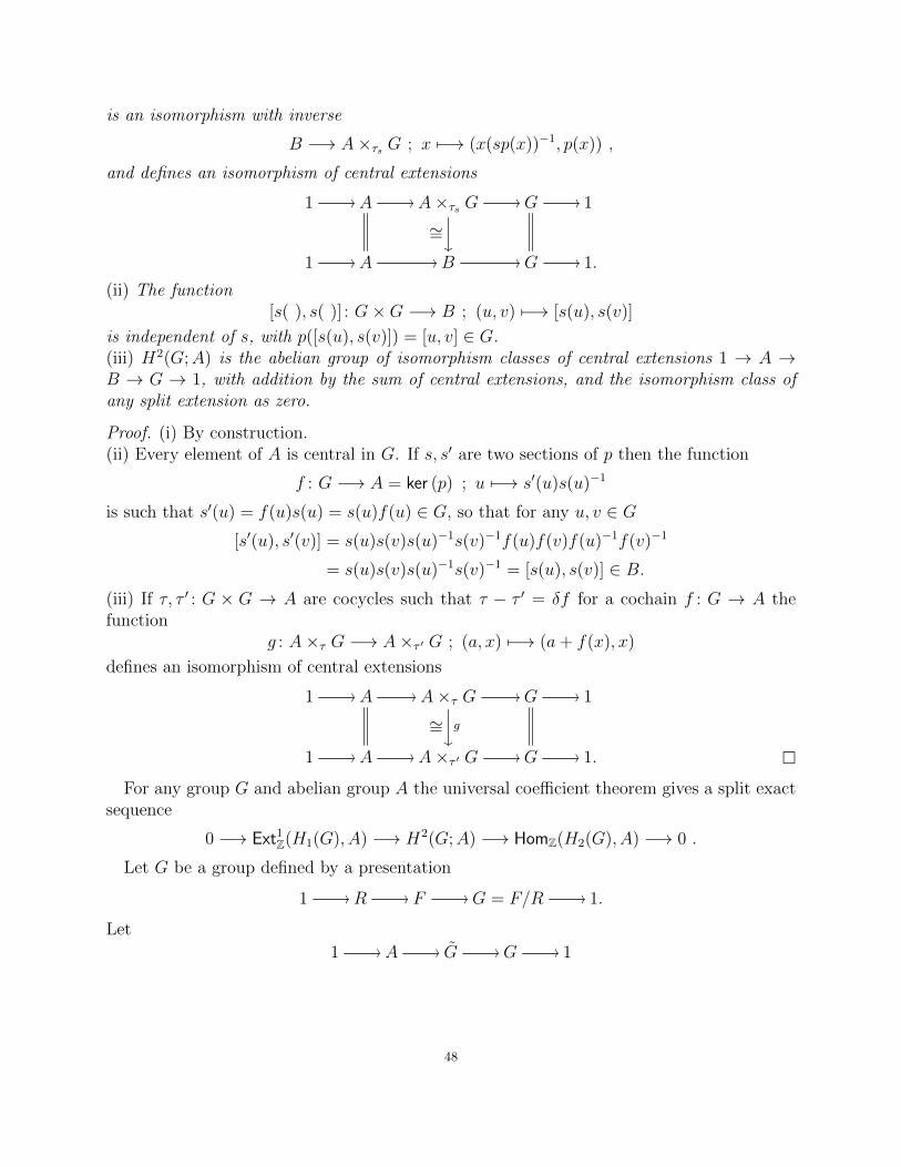
is an isomorphism with inverse
B −→ A×τs G ; x 7−→ (x(sp(x))−1, p(x)) ,
and defines an isomorphism of central extensions
1 // A // A×τs G∼=
// G // 1
1 // A // B // G // 1.
(ii) The function[s( ), s( )] : G×G −→ B ; (u, v) 7−→ [s(u), s(v)]
is independent of s, with p([s(u), s(v)]) = [u, v] ∈ G.(iii) H2(G;A) is the abelian group of isomorphism classes of central extensions 1 → A →B → G → 1, with addition by the sum of central extensions, and the isomorphism class ofany split extension as zero.
Proof. (i) By construction.(ii) Every element of A is central in G. If s, s′ are two sections of p then the function
f : G −→ A = ker (p) ; u 7−→ s′(u)s(u)−1
is such that s′(u) = f(u)s(u) = s(u)f(u) ∈ G, so that for any u, v ∈ G[s′(u), s′(v)] = s(u)s(v)s(u)−1s(v)−1f(u)f(v)f(u)−1f(v)−1
= s(u)s(v)s(u)−1s(v)−1 = [s(u), s(v)] ∈ B.(iii) If τ, τ ′ : G × G → A are cocycles such that τ − τ ′ = δf for a cochain f : G → A thefunction
g : A×τ G −→ A×τ ′ G ; (a, x) 7−→ (a+ f(x), x)
defines an isomorphism of central extensions
1 // A // A×τ Gg∼=
// G // 1
1 // A // A×τ ′ G // G // 1.
For any group G and abelian group A the universal coefficient theorem gives a split exactsequence
0 −→ Ext1Z(H1(G), A) −→ H2(G;A) −→ HomZ(H2(G), A) −→ 0 .
Let G be a group defined by a presentation
1 // R // F // G = F/R // 1.
Let
1 // A // G // G // 1
48
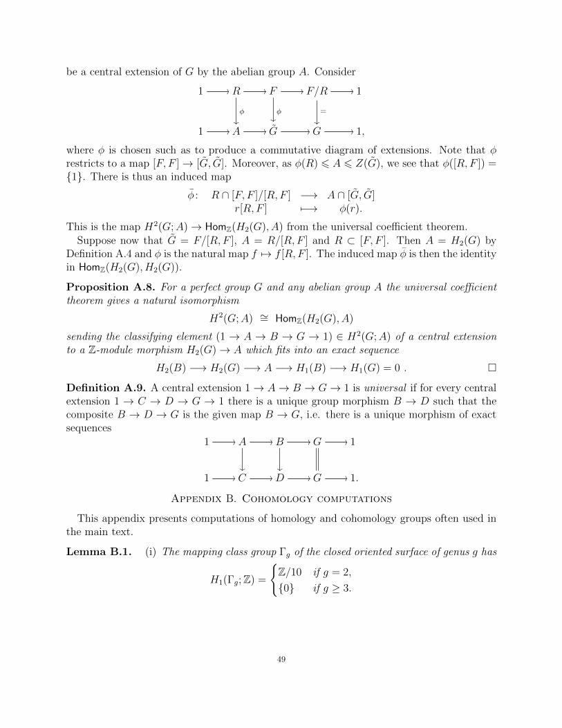
be a central extension of G by the abelian group A. Consider
1 // R //
φ
F //
φ
F/R //
=
1
1 // A // G // G // 1,
where φ is chosen such as to produce a commutative diagram of extensions. Note that φrestricts to a map [F, F ]→ [G, G]. Moreover, as φ(R) 6 A 6 Z(G), we see that φ([R,F ]) =1. There is thus an induced map
φ : R ∩ [F, F ]/[R,F ] −→ A ∩ [G, G]r[R,F ] 7−→ φ(r).
This is the map H2(G;A)→ HomZ(H2(G), A) from the universal coefficient theorem.Suppose now that G = F/[R,F ], A = R/[R,F ] and R ⊂ [F, F ]. Then A = H2(G) by
Definition A.4 and φ is the natural map f 7→ f [R,F ]. The induced map φ is then the identityin HomZ(H2(G), H2(G)).
Proposition A.8. For a perfect group G and any abelian group A the universal coefficienttheorem gives a natural isomorphism
H2(G;A) ∼= HomZ(H2(G), A)
sending the classifying element (1 → A → B → G → 1) ∈ H2(G;A) of a central extensionto a Z-module morphism H2(G)→ A which fits into an exact sequence
H2(B) −→ H2(G) −→ A −→ H1(B) −→ H1(G) = 0 .
Definition A.9. A central extension 1→ A→ B → G→ 1 is universal if for every centralextension 1 → C → D → G → 1 there is a unique group morphism B → D such that thecomposite B → D → G is the given map B → G, i.e. there is a unique morphism of exactsequences
1 // A
// B
// G // 1
1 // C // D // G // 1.
Appendix B. Cohomology computations
This appendix presents computations of homology and cohomology groups often used inthe main text.
Lemma B.1. (i) The mapping class group Γg of the closed oriented surface of genus g has
H1(Γg;Z) =
Z/10 if g = 2,
0 if g ≥ 3.
49
Indeed, the mapping class groups are perfect ∀g ≥ 3.
H2(Γg;Z) =
Z/2 if g = 2,
Z⊕ Z/2 if g = 3,
Z if g ≥ 4.
H2(Γg;Z) =
Z/10 if g = 2,
Z if g ≥ 3.
H2(Γg;Z/2) =
Z/2⊕ Z/2 if g = 2, 3,
Z/2 if g ≥ 4.
(ii)
H1(Sp(2g,Z);Z) =
Z/2 if g = 2,
0 if g ≥ 3.
H1(Sp(2g,Z/4);Z) =
Z/2 if g = 2,
0 if g ≥ 3.
In fact, the symplectic group Sp(2g,Z) and thus all of its quotients, as quotients of themapping class group, are perfect ∀g ≥ 3.
(iii)
H2(Sp(2g,Z);Z) =
Z⊕ Z/2 if g = 2, 3,
Z if g ≥ 4.
(iv)
H2(Sp(2g,Z/4);Z) =
Z/2⊕ Z/2 if g = 2, 3,
Z/2 if g ≥ 4.
(v)
H2(Sp(2g,Z);Z) =
Z⊕ Z/2 if g = 2,
Z if g ≥ 3.
(vi)
H2(Sp(2g,Z);Z/2) =
Z/2⊕ Z/2⊕ Z/2 if g = 2,
Z/2⊕ Z/2 if g = 3,
Z/2 if g ≥ 4.
(vii)
H2(Sp(2g,Z);Z/8) =
Z/8⊕ Z/2⊕ Z/2 if g = 2,
Z/8⊕ Z/2 if g = 3,
Z/8 if g ≥ 4.
(viii)
H2(Sp(2g,Z/4);Z/2) =
Z/2⊕ Z/2⊕ Z/2 if g = 2,
Z/2⊕ Z/2 if g = 3,
Z/2 if g ≥ 4.
50
(ix)
H2(Sp(2g,Z/4);Z/8) =
Z/2⊕ Z/2⊕ Z/2 if g = 2,
Z/2⊕ Z/2 if g = 3,
Z/2 if g ≥ 4.
(x) The image of the map r2 : H2(Sp(2g,Z);Z)→ H2(Sp(2g,Z);Z/2) isZ/2⊕ Z/2⊕ 0 if g = 2,
Z/2⊕ 0 if g = 3,
Z/2 if g ≥ 4.
(xi) The image of the map r8 : H2(Sp(2g,Z);Z)→ H2(Sp(2g,Z);Z/8) isZ/8⊕ Z/2⊕ 0 if g = 2,
Z/8⊕ 0 if g = 3,
Z/8 if g ≥ 4.
(xii) The map p∗ : H2(Γg;Z) → H2(Sp(2g,Z);Z) induced in homology by the canonical sur-jection p : Γg → Sp(2g,Z) is an isomorphism for g ≥ 3.
(xiii) The map p∗ : H2(Sp(2g,Z);Z) → H2(Γg;Z) induced in cohomology by the canonicalsurjection p : Γg → Sp(2g,Z) is an isomorphism for g ≥ 3.
(xiv) The map p∗ : H2(Sp(2g,Z);Z/2)→ H2(Γg;Z/2) induced in cohomology by the canonicalsurjection p : Γg → Sp(2g,Z) is an isomorphism for g ≥ 3.
Proof. (i) For g = 2, we have H1(Γ2;Z) = Z/10 (see for example [22, Theorem 5.1]).For H2(Γ2;Z) see [22, after Theorem 6.1]. The universal coefficient theorem and theproperties of Ext allow to easily compute H2(Γ2;Z) and H2(Γ2;Z/2).
For g ≥ 3, we have H1(Γg;Z) = 0 (see for example [14, Theorem 5.2]). The groupH2(Γ3;Z) is computed in [35, Corollary 4.10]. For g ≥ 4, we have H2(Γg;Z) = Z(see for example [22, Theorem 6.1]). From that we easily obtain H2(Γg;Z) andH2(Γg;Z/2) using the universal coefficient theorem.
(ii) The symplectic group Sp(2g,Z), and thus all of its quotients, is a quotient of themapping class group Γg, which is perfect for g ≥ 3 (see for example [14, Theorems5.2, 6.4]).
For g = 2, one can abelianize the presentation of Sp(4,Z) given in [3] or [25,Theorem 2].
For Sp(4,Z/4), one can compute it using GAP.(iii) See for example [5, Lemma 6.11] for g ≥ 3.
For g = 2 it was computed using GAP.(iv) See for example [5, Lemma 6.12] for g ≥ 3.
For g = 2, it can be computed using GAP.(v) For g ≥ 3, perfection of Sp(2g,Z) together with the universal coefficient theorem
gives an isomorphism
H2(Sp(2g,Z);Z)∼=// Hom(H2(Sp(2g,Z);Z),Z).
Hence using (iii) we obtain the stated cohomology group.51
For g = 2, the universal coefficient theorem gives a split exact sequence
Ext1Z(H1(Sp(4,Z);Z),Z) // H2(Sp(4,Z);Z) // Hom(H2(Sp(4,Z);Z),Z).
Using (ii), (iii) together with the properties of Ext, one obtains H2(Sp(4,Z);Z) ∼=Z⊕ Z/2 as stated.
(vi) For g ≥ 3, perfection of Sp(2g,Z) together with the universal coefficient theoremgives an isomorphism
H2(Sp(2g,Z);Z/2)∼=// Hom(H2(Sp(2g,Z);Z),Z/2).
Hence using (iii) we obtain the stated cohomology groups.For g = 2, the universal coefficient theorem yields the split exact sequence
Ext1Z(H1(Sp(2g,Z);Z),Z/2) // H2(Sp(2g,Z);Z/2) // Hom(H2(Sp(2g,Z);Z),Z/2).
Using (ii) and (iii) and the properties of Ext we obtain the required results.(vii) For g ≥ 3, perfection of Sp(2g,Z) together with the universal coefficient theorem
gives an isomorphism
H2(Sp(2g,Z);Z/8)∼=// Hom(H2(Sp(2g,Z);Z),Z/8).
Hence using (iii) we obtain the stated cohomology groups.For g = 2, the universal coefficient theorem yields the split exact sequence
Ext1Z(H1(Sp(2g,Z);Z),Z/8) // H2(Sp(2g,Z);Z/8) // Hom(H2(Sp(2g,Z);Z),Z/8).
Using (ii) and (iii) and the properties of Ext we obtain the required results.(viii) For g ≥ 3, perfection of Sp(2g,Z/4) together with the universal coefficient theorem
gives an isomorphism
H2(Sp(2g,Z/4);Z/2)∼=// Hom(H2(Sp(2g,Z/4);Z),Z/2).
Hence using (iv) we obtain the stated cohomology groups.For g = 2, the universal coefficient theorem yields the split exact sequence
Ext1Z(H1(Sp(2g,Z/4);Z),Z/2) // H2(Sp(2g,Z/4);Z/2) // Hom(H2(Sp(2g,Z/4);Z),Z/2).
Points (ii) and (iv) and the properties of the Ext-functor yield the stated results.(ix) For g ≥ 3, perfection of Sp(2g,Z/4) together with the universal coefficient theorem
gives an isomorphism
H2(Sp(2g,Z/4);Z/8)∼=// Hom(H2(Sp(2g,Z/4);Z),Z/8).
Hence using (iv) we obtain the stated cohomology groups.For g = 2, the universal coefficient theorem yields the split exact sequence
Ext1Z(H1(Sp(2g,Z/4);Z),Z/8) // H2(Sp(2g,Z/4);Z/8) // Hom(H2(Sp(2g,Z/4);Z),Z/8).
Points (ii) and (iv) and the properties of the Ext-functor yield the stated results.
52
(x) Naturality of the universal coefficient theorem and perfection of Sp(2g,Z) for g ≥ 3give a commutative diagram
H2(Sp(2g,Z);Z)∼=//
r2
Hom(H2(Sp(2g,Z);Z),Z)
H2(Sp(2g,Z);Z/2)∼=// Hom(H2(Sp(2g,Z);Z),Z/2).
For g = 2, the universal coefficient theorem yields the split exact sequence
Ext1Z(H1(Sp(4,Z);Z),Z) //
H2(Sp(4,Z);Z) //
r2
Hom(H2(Sp(4,Z);Z),Z)
Ext1Z(H1(Sp(4,Z);Z),Z/2) // H2(Sp(4,Z);Z/2) // Hom(H2(Sp(4,Z);Z),Z/2).
It is easy to understand the map induced by r2 on the Hom-part: it is just theconcatenation with the reduction morphism on the coefficients Z→ Z/2.
For the Ext-part, consider the projective resolution of H1(Sp(4,Z),Z) = Z/2 givenby
0 −→ Z ·2−→ Z −→ Z/2 −→ 0.
Apply Hom to obtain
0 Hom(Z,Z)oo
r
Hom(Z,Z)
·2oo
0 Hom(Z,Z/2)oo Hom(Z,Z/2).·2oo
The groups we are interested in, Ext1Z(H1(Sp(4,Z);Z),Z) and Ext1Z(H1(Sp(4,Z);Z),Z/2),are the cohomology groups of this part of the chain complexes. We notice that themap induced in cohomology is surjective, as the map r is.
The map r2 thus has imageZ/2⊕ Z/2⊕ 0 if g = 2,
Z/2⊕ 0 if g = 3,
Z/2 if g ≥ 4.
(xi) Naturality of the universal coefficient theorem and perfection of Sp(2g,Z) for g ≥ 3give a commutative diagram
H2(Sp(2g,Z);Z)∼=//
r8
Hom(H2(Sp(2g,Z);Z),Z)
H2(Sp(2g,Z);Z/8)∼=// Hom(H2(Sp(2g,Z);Z),Z/8).
53
For g = 2, the universal coefficient theorem yields the split exact sequence
Ext1Z(H1(Sp(4,Z);Z),Z) //
H2(Sp(4,Z);Z) //
r8
Hom(H2(Sp(4,Z);Z),Z)
Ext1Z(H1(Sp(4,Z);Z),Z/8) // H2(Sp(4,Z);Z/8) // Hom(H2(Sp(4,Z);Z),Z/8).
It is easy to understand the map induced by r8 on the Hom-part: it is just theconcatenation with the reduction morphism on the coefficients Z→ Z/8.
For the Ext-part, consider the projective resolution of H1(Sp(4,Z);Z) = Z/2 givenby
0 −→ Z ·2−→ Z −→ Z/2 −→ 0.
Apply Hom to obtain
0 Hom(Z,Z)oo
r
Hom(Z,Z)
·2oo
0 Hom(Z,Z/8)oo Hom(Z,Z/8).·2oo
The groups we are interested in, Ext1Z(H1(Sp(4,Z);Z),Z) and Ext1Z(H1(Sp(4,Z);Z),Z/8),are the cohomology groups of this part of the chain complexes. We notice that themap induced in cohomology is surjective, as the map r is.
The map r8 thus has imageZ/2⊕ Z/8⊕ 0 if g = 2,
Z/8⊕ 0 if g = 3,
Z/8 if g ≥ 4.
(xii) Meyer shows in [29, Satz 2] that the image of the cocycle τg under the compositionof
HomZ(H2(Sp(2g,Z);Z),Z) ∼= H2(Sp(2g,Z);Z) // H2(Γg;Z)∼=// HomZ(H2(Γg;Z),Z)
is a map k ∈ HomZ(H2(Γg;Z),Z) with image 4Z. On the other hand, Barge-Ghysshow in [1, Proposition 3.1, p. 258] that τg is four times the cocycle defined by the cen-
tral extension ˜Sp(2g,Z), the restriction of the universal cover ˜Sp(2g,R) of Sp(2g,R)to Sp(2g,Z). This means that τg is four times the generator of H2(Sp(2g,Z);Z),which maps to four times the generator of H2(Γg;Z). Now this means that the re-striction of p∗ to the Z-summand of H2(Γg;Z) is an isomorphism to the Z-summandof H2(Sp(2g,Z);Z).
The case g ≥ 4 is thus settled. For g = 3, we use Theorem 4.9, Corollary 4.10and the paragraph before in [35], together with [23, Proposition 1.5]: the mapH2(Γ3,1;Z) → H2(Γ3;Z) is surjective, thus an isomorphism, and this implies thatthe Z/2-summand of H2(Γ3;Z) is sent isomorphically by p∗ to the Z/2-summand ofH2(Sp(6,Z);Z). The proof of the isomorphism is now complete.
54
(xiii) Meyer shows in [29, Satz 2] that the image of the cocycle τg under the compositionof
H2(Sp(2g,Z);Z) // H2(Γg;Z) // HomZ(H2(Γg;Z),Z)
is a map k ∈ HomZ(H2(Γg;Z),Z) with image 4Z. On the other hand, Barge-Ghysshow in [1, Proposition 3.1, p. 258] that τg is four times the cocycle defined by the cen-
tral extension ˜Sp(2g,Z), the restriction of the universal cover ˜Sp(2g,R) of Sp(2g,R) toSp(2g,Z). This means that τg is four times the generator of H2(Sp(2g,Z);Z), whichmaps to four times the generator of H2(Γg;Z), showing that p∗ is an isomorphism.
(xiv) We showed above that p∗ : H2(Γg;Z)→ H2(Sp(2g,Z);Z) is an isomorphism for g ≥ 3.The universal coefficient theorem and perfection of Γg and Sp(2g,Z) yield a commu-tative diagram
H2(Sp(2g,Z);Z/2)∼=//
p∗
Hom(H2(Sp(2g,Z);Z),Z/2)
Hom(p∗)
H2(Γg;Z/2)∼=
// Hom(H2(Γg;Z),Z/2).
The left vertical arrow must therefore be an isomorphism as well.For g = 2, recall that by (i) and (vi) the map p∗ cannot possibly be an isomorphism.
We use the following commutative diagram to study its kernel:
H2(Sp(4,Z);Z)r2//
p∗
H2(Sp(4,Z);Z/2)
p∗
H2(Γ2;Z) // H2(Γ2;Z/2).
The class [τ2] ∈ H2(Sp(4,Z);Z) has non-zero image
r2([τ2]) = [τ2] (mod 2) ∈ H2(Sp(4,Z);Z/2)
by (x), from which it follows also that this image has order 2. By [29, Satz 2], theorder of p∗([τ2]) is 5 in H2(Γ2;Z). But then its image in H2(Γ2;Z/2) has to be 0, by(i). So p∗ : H2(Sp(4,Z);Z/2) → H2(Γ2;Z/2) is not injective and has r2([τ2]) in itskernel.
Appendix C. Werner Meyer (by Winfried Scharlau)
We are grateful to Winfried Scharlau for allowing us to publish here his photo of Meyer,and the following English translation of an extract from his 2017 biography of Hirzebruch,[36].
55
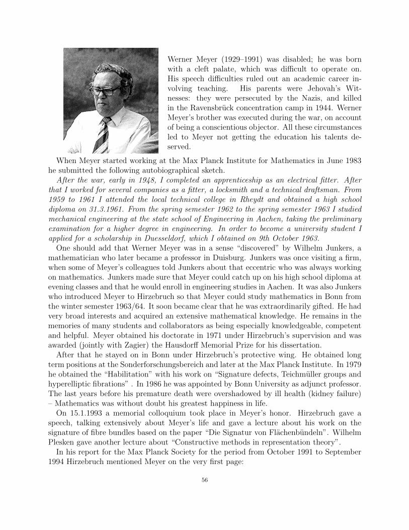
Werner Meyer (1929–1991) was disabled; he was bornwith a cleft palate, which was difficult to operate on.His speech difficulties ruled out an academic career in-volving teaching. His parents were Jehovah’s Wit-nesses: they were persecuted by the Nazis, and killedin the Ravensbruck concentration camp in 1944. WernerMeyer’s brother was executed during the war, on accountof being a conscientious objector. All these circumstancesled to Meyer not getting the education his talents de-served.
When Meyer started working at the Max Planck Institute for Mathematics in June 1983he submitted the following autobiographical sketch.
After the war, early in 1948, I completed an apprenticeship as an electrical fitter. Afterthat I worked for several companies as a fitter, a locksmith and a technical draftsman. From1959 to 1961 I attended the local technical college in Rheydt and obtained a high schooldiploma on 31.3.1961. From the spring semester 1962 to the spring semester 1963 I studiedmechanical engineering at the state school of Engineering in Aachen, taking the preliminaryexamination for a higher degree in engineering. In order to become a university student Iapplied for a scholarship in Duesseldorf, which I obtained on 9th October 1963.
One should add that Werner Meyer was in a sense “discovered” by Wilhelm Junkers, amathematician who later became a professor in Duisburg. Junkers was once visiting a firm,when some of Meyer’s colleagues told Junkers about that eccentric who was always workingon mathematics. Junkers made sure that Meyer could catch up on his high school diploma atevening classes and that he would enroll in engineering studies in Aachen. It was also Junkerswho introduced Meyer to Hirzebruch so that Meyer could study mathematics in Bonn fromthe winter semester 1963/64. It soon became clear that he was extraordinarily gifted. He hadvery broad interests and acquired an extensive mathematical knowledge. He remains in thememories of many students and collaborators as being especially knowledgeable, competentand helpful. Meyer obtained his doctorate in 1971 under Hirzebruch’s supervision and wasawarded (jointly with Zagier) the Hausdorff Memorial Prize for his dissertation.
After that he stayed on in Bonn under Hirzebruch’s protective wing. He obtained longterm positions at the Sonderforschungsbereich and later at the Max Planck Institute. In 1979he obtained the “Habilitation” with his work on “Signature defects, Teichmuller groups andhyperelliptic fibrations” . In 1986 he was appointed by Bonn University as adjunct professor.The last years before his premature death were overshadowed by ill health (kidney failure)– Mathematics was without doubt his greatest happiness in life.
On 15.1.1993 a memorial colloquium took place in Meyer’s honor. Hirzebruch gave aspeech, talking extensively about Meyer’s life and gave a lecture about his work on thesignature of fibre bundles based on the paper “Die Signatur von Flachenbundeln”. WilhelmPlesken gave another lecture about “Constructive methods in representation theory”.
In his report for the Max Planck Society for the period from October 1991 to September1994 Hirzebruch mentioned Meyer on the very first page:
56
“He was able to go deep into the matter. In some lectures and seminars about new researchI used to set problems that I couldn’t solve myself, promising a bottle of wine to whoever couldgive a solution. Many times the prize went to Werner Meyer. With his great knowledge hewas an outstanding advisor for Masters and Doctoral candidates. He helped many studentseven if they were not writing their dissertation officially with him.”
References
[1] J. Barge, E. Ghys, Cocycles d’Euler et de Maslov, Math. Ann. 294 (1992), no. 2, 235–265.[2] S. Baaj, G. Skandalis, and S. Vaes, Measurable Kac Cohomology for Bicrossed Products, Trans. Amer.
Math. Soc. 357 (November 2004), no. 4, 1497–1524.[3] P. Bender, Eine Prasentation der symplektischen Gruppe Sp(4,Z) mit 2 Erzeungenden und 8 definieren-
den Relationen, J. Algebra 65 (1980), no. 2, 328–331.[4] D. J. Benson, Theta functions and a presentation of 21+(2g+1)Sp(2g, 2), preprint
http://homepages.abdn.ac.uk/d.j.benson/html/archive/benson.html, 2017.[5] , C. Campagnolo, A. Ranicki, and C. Rovi, Cohomology of symplectic groups and Meyer’s sig-
nature theorems, preprint http://arxiv.org/abs/1710.04851, 2017.[6] F. R. Beyl, The Schur multiplicator of SL(2,Z/mZ) and the Congruence Subgroup Property, Math. Z.
191 (1986), no. 1, 23–42.[7] K. S. Brown, Cohomology of Groups, Springer (1982).[8] C. Campagnolo, Surface bundles over surfaces: A study through signature and simplicial volume,
10.13097/archive-ouverte/unige:96380, 2016.[9] I. Chatterji, Y. de Cornulier, G. Mislin, and C. Pittet, Bounded characteristic classes and flat bundles,
J. Differential. Geom. 95 (2013), no. 1, 39–51.[10] I. Chatterji, G. Mislin, C. Pittet, and L. Saloff-Coste, A geometric criterion for the boundedness of
characteristic classes, Math. Ann. 351 (2011), no. 3, 541–569.[11] S. S. Chern, F. Hirzebruch, J.-P. Serre, On the Index of a Fibered Manifold, Proceedings of the American
Mathematical Society 8 (Jun., 1957), no. 3, 587–596.[12] J. H. Conway, R. Turner Curtis, S. P. Norton, R. A. Parker, and R. Arnott Wilson, Atlas of Finite
Groups. Maximal Subgroups and Ordinary Characters for Simple Groups, Oxford University Press, 1985.[13] P. Deligne, Extensions centrales non residuellement finies des groupes arithmetiques, C. R. Acad. Sci.
Paris, Ser. A-B 287 (1978), no. 4, A203–A208.[14] B. Farb and D. Margalit, A primer on mapping class groups, Princeton (2012).[15] S. Galatius and O. Randal-Williams, Abelian quotients of mapping class groups of highly connected
manifolds, Math. Ann. 365 (2016), no. 1-2, 857–879.[16] P. Gilmer and G. Masbaum, Maslov index, lagrangians, mapping class groups and TQFT, Forum Math.
25 (2013), no. 5, 1067–1106.[17] R. L. Griess, Automorphisms of extra special groups and nonvanishing degree 2 cohomology, Pacific J.
Math. 48 (1973), no. 2, 403–422.[18] I. Hambleton, A. Korzeniewski, and A. Ranicki, The signature of a fibre bundle is multiplicative mod 4,
Geom. Topol. 11 (2007), 251–314.[19] G. Hochschild, The Structure of Lie Groups, Holden-Day (1965).[20] H. Hopf, Fundamentalgruppe und zweite Bettische Gruppe, Comment. Math. Helv. 14 (1942), 257–309.[21] R. Kirby and P. Melvin, Dedekind sums, µ-invariants and the signature cocycle, Math. Ann. 299 (1994),
no. 2, 231–267.[22] M. Korkmaz, Low-dimensional homology groups of mapping class groups: a survey, Turkish J. Math.
26 (2002), no. 1, 101–114.[23] M. Korkmaz and A. I. Stipsicz, The second homology groups of mapping class groups of orientable
surfaces, Math. Proc. Cambridge Philos. Soc. 134 (2003), no. 3, 479–489.[24] J. Leray, Lagrangian analysis and quantum mechanics, MIT Press (1981).[25] N. Lu, A Simple presentation of the Siegel Modular Groups, Linear Algebra Appl. 166 (1992), 185–194.
57
[26] G. W. Mackey, Borel structure in groups and their duals, Trans. Amer. Math. Soc. 85 (1957), 134–165.[27] V. P. Maslov, Theorie des perturbations et methodes asymptotiques, Dunod (1972 (transl. of 1965 Russian
edition)).[28] W. Meyer, Die Signatur von lokalen Koeffizientensystemen und Faserbundeln., Bonn. Math. Schr. No.
53 (1972), viii+59, http://www.maths.ed.ac.uk/ aar/papers/meyerthesis.pdf[29] W. Meyer, Die Signatur von Flachenbundeln, Math. Ann. 201 (1973), 239–264.[30] J. Milnor, On the homology of Lie groups made discrete, Comment. Math. Helv. 58 (1983), no. 1, 72–85.[31] C. C. Moore, Group Extensions and Cohomology for Locally Compact Groups. III, Trans. Amer. Math.
Soc. 221 (July 1976), no. 1, 1–33.[32] P. Py, Indice de Maslov et Theoreme de Novikov–Wall, Bol. Soc. Mat. Mexicana (3) 11 (2005), no. 2,
303–331.[33] C. Rovi, The non-multiplicativity of the signature modulo 8 of a fibre bundle is an Arf–Kervaire invariant,
Algebr. Geom. Topol. 18 (2018), 1281–1322.[34] C.-H. Sah and J. B. Wagoner, Second homology of Lie groups made discrete, Comm. Algebra 5 (1977),
no. 6, 611–642.[35] T. Sakasai, Lagrangian mapping class groups from a group cohomological point of view, Algebr. Geom.
Topol. 12 (2012), no. 1, 267–291.[36] W. Scharlau, Das Gluck, Mathematiker zu sein. Friedrich Hirzebruch und seine Zeit, Heidelberg:
Springer Spektrum (2017).
[37] J. Schur, Uber die Darstellung der endlichen Gruppen durch gebrochene lineare Substitutionen, J. reineangew. Math. 127 (1904), 20–50.
[38] W. Thurston, Foliations and groups of diffeomorphisms, Bull. Amer. Math. Soc. 80 (1974), 304–307.[39] C. T. C. Wall, Non-additivity of the signature, Invent. Math, 7 (1969), 269–274.[40] A. Weil, L’integration dans les groupes topologiques et ses applications, Hermann, Paris (1940).[41] D. Wigner, Algebraic Cohomology of Topological Groups, Trans. Amer. Math. Soc. 178 (April 1973),
83–93.
Institute of Mathematics, University of Aberdeen, Aberdeen AB24 3UE, Scotland, UnitedKingdom
Department of Mathematics, Karlsruhe Institute of Technology, D-76128 Karlsruhe,Germany
School of Mathematics, University of Edinburgh, Edinburgh EH9 3FD, Scotland, UnitedKingdom
Department of Mathematics, Indiana University, Bloomington IN 47405, USA
58

![A primer on computational group homology and …arXiv:0706.0549v2 [math.GR] 10 Jun 2009 A primer on computational group homology and cohomology using GAPand SAGE ∗ David Joyner†](https://img.pdfslide.us/doc/110x75/5e867d96b392c82caa4664de/a-primer-on-computational-group-homology-and-arxiv07060549v2-mathgr-10-jun.jpg)


![LOCALIZATION OF EILENBERG-MACLANE G-SPACES WITH …homology theories and ordinary homology and cohomology theories in § 1, following Wilson [16]. Given a homology theory h% and a](https://img.pdfslide.us/doc/110x75/5edc8695ad6a402d6667388f/localization-of-eilenberg-maclane-g-spaces-with-homology-theories-and-ordinary-homology.jpg)
![Equivariant homology and cohomology of groups · theory of groups with operators corresponding to the cohomology theory of groups with operators [8] has been treated in [11]. In [8]](https://img.pdfslide.us/doc/110x75/5f700fcec725c371f133f0aa/equivariant-homology-and-cohomology-of-groups-theory-of-groups-with-operators-corresponding.jpg)


![Homology Flows, Cohomology Cutsjeffe.cs.illinois.edu/pubs/pdf/surflow.pdf · 2 Homology Flows, Cohomology Cuts algorithm known for integer capacities, due to Goldberg and Rao [48],](https://img.pdfslide.us/doc/110x75/5edaec2909ac2c67fa688660/homology-flows-cohomology-2-homology-flows-cohomology-cuts-algorithm-known-for.jpg)


![Whitney homology, cohomology and Steenrod squaresmurolo/ Mes.Articles.pdf/Whitney.Hom... · Whitney homology, cohomology and Steenrod squares CLAUDIO MUROLO (*) Abstract.–In[1]](https://img.pdfslide.us/doc/110x75/5c6780d209d3f2034d8c0414/whitney-homology-cohomology-and-steenrod-squares-murolo-mes-whitney-homology.jpg)