Embed Size (px)
Citation preview

Introduction: Goals
Introduction
Goals Rationale HowTo Examples
This lecture will help you understand what a root locus is and how to create and use one. It provides definitions of terms, a step-by-step guide to constructing a root locus, and details about how to design and evaluate controllers using the root locus method.
After studying these materials, you should be able to create a root locus and use the locus to understand the closed-loop system behavior given an open-loop system and a feedback controller.
Root Locus
IntroductionDefinitions Angle Criterion Angle of Departure Break Point Characteristic Equation Closed-Loop Complex-Plane (s-plane) Forward Loop Magnitude Criterion Open-Loop Root Locus Root Locus Gain Routh-Hurwitz Criterion Transfer FunctionConstructing the Locus Step 1: Open-Loop Roots Step 2: Real Axis Crossings Step 3: Asymptotes Step 4: Breakpoints Step 5: Angles of Departure/Arrival Step 6: Axis Crossings Step 7: Sketch the LocusCalculating the GainCase Studies MagLev Train Steel-Rolling Mill Robot Arm
http://me.mit.edu/lectures/rlocus/1-goals.html (1 of 2)9/29/2005 2:59:18 PM
Root Locus: Rationale
Root Locus
Goals Rationale HowTo Examples
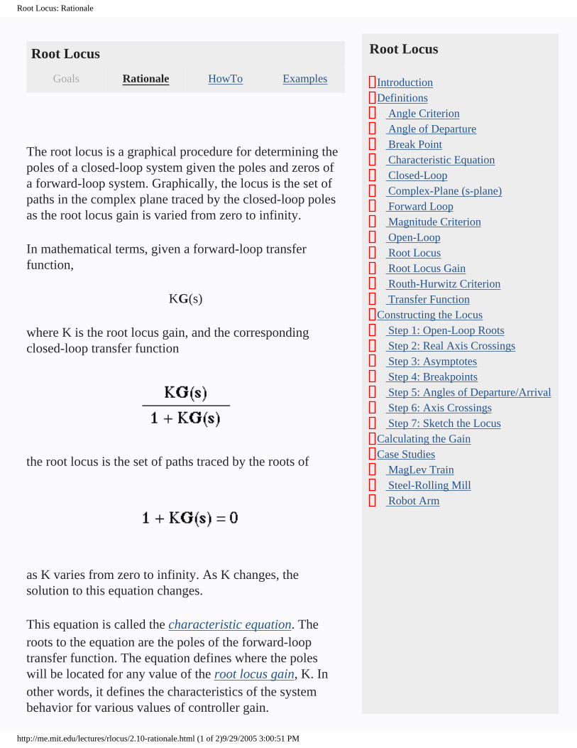
The root locus is a graphical procedure for determining the poles of a closed-loop system given the poles and zeros of a forward-loop system. Graphically, the locus is the set of paths in the complex plane traced by the closed-loop poles as the root locus gain is varied from zero to infinity.
In mathematical terms, given a forward-loop transfer function,
KG(s)
where K is the root locus gain, and the corresponding closed-loop transfer function
the root locus is the set of paths traced by the roots of
as K varies from zero to infinity. As K changes, the solution to this equation changes.
This equation is called the characteristic equation. The roots to the equation are the poles of the forward-loop transfer function. The equation defines where the poles will be located for any value of the root locus gain, K. In other words, it defines the characteristics of the system behavior for various values of controller gain.
Root Locus
IntroductionDefinitions Angle Criterion Angle of Departure Break Point Characteristic Equation Closed-Loop Complex-Plane (s-plane) Forward Loop Magnitude Criterion Open-Loop Root Locus Root Locus Gain Routh-Hurwitz Criterion Transfer FunctionConstructing the Locus Step 1: Open-Loop Roots Step 2: Real Axis Crossings Step 3: Asymptotes Step 4: Breakpoints Step 5: Angles of Departure/Arrival Step 6: Axis Crossings Step 7: Sketch the LocusCalculating the GainCase Studies MagLev Train Steel-Rolling Mill Robot Arm
http://me.mit.edu/lectures/rlocus/2.10-rationale.html (1 of 2)9/29/2005 3:00:51 PM

Root Locus: Rationale
block diagram of the closed loop system
http://me.mit.edu/lectures/rlocus/2.10-rationale.html (2 of 2)9/29/2005 3:00:51 PM
Characteristic Equation: Rationale
Characteristic Equation
Goals Rationale HowTo Examples
The characteristic equation of a system is based upon the the transfer function that models the system. It contains information needed to determine the response of a dynamic system. There is only one characteristic equation for a given system.
Root Locus
IntroductionDefinitions Angle Criterion Angle of Departure Break Point Characteristic Equation Closed-Loop Complex-Plane (s-plane) Forward Loop Magnitude Criterion Open-Loop Root Locus Root Locus Gain Routh-Hurwitz Criterion Transfer FunctionConstructing the Locus Step 1: Open-Loop Roots Step 2: Real Axis Crossings Step 3: Asymptotes Step 4: Breakpoints Step 5: Angles of Departure/Arrival Step 6: Axis Crossings Step 7: Sketch the LocusCalculating the GainCase Studies MagLev Train Steel-Rolling Mill Robot Arm
http://me.mit.edu/lectures/rlocus/2.4-rationale.html (1 of 2)9/29/2005 3:01:35 PM

Root Locus Gain: Rationale
Root Locus Gain
Goals Rationale HowTo Examples
The root locus gain, typically denoted as K, is a gain of the forward-loop system. While determining the root locus, this gain is varied from 0 to infinity. Note that the corresponding variations in the poles of the closed-loop system determine the root locus. As the gain moves from 0 to infinity, the poles move from the forward-loop poles along the locus toward forward-loop zeros or infinity.
In block diagram form, the root locus gain is located in the forward loop, before the system, as shown below.
Root Locus
IntroductionDefinitions Angle Criterion Angle of Departure Break Point Characteristic Equation Closed-Loop Complex-Plane (s-plane) Forward Loop Magnitude Criterion Open-Loop Root Locus Root Locus Gain Routh-Hurwitz Criterion Transfer FunctionConstructing the Locus Step 1: Open-Loop Roots Step 2: Real Axis Crossings Step 3: Asymptotes Step 4: Breakpoints Step 5: Angles of Departure/Arrival Step 6: Axis Crossings Step 7: Sketch the LocusCalculating the GainCase Studies MagLev Train Steel-Rolling Mill Robot Arm
http://me.mit.edu/lectures/rlocus/2.11-rationale.html (1 of 2)9/29/2005 3:02:26 PM

Definitions: Rationale
Definitions
Goals Rationale HowTo Examples
This section contains definitions of root locus terms and concepts. If these definitions do not adequately answer your questions, please consult the prerequisites for this lecture.
Root Locus
IntroductionDefinitions Angle Criterion Angle of Departure Break Point Characteristic Equation Closed-Loop Complex-Plane (s-plane) Forward Loop Magnitude Criterion Open-Loop Root Locus Root Locus Gain Routh-Hurwitz Criterion Transfer FunctionConstructing the Locus Step 1: Open-Loop Roots Step 2: Real Axis Crossings Step 3: Asymptotes Step 4: Breakpoints Step 5: Angles of Departure/Arrival Step 6: Axis Crossings Step 7: Sketch the LocusCalculating the GainCase Studies MagLev Train Steel-Rolling Mill Robot Arm
http://me.mit.edu/lectures/rlocus/2-rationale.html (1 of 2)9/29/2005 3:03:13 PM

Definitions: Rationale
http://me.mit.edu/lectures/rlocus/2-rationale.html (2 of 2)9/29/2005 3:03:13 PM
Root Locus : Pre-Requisites
Root Locus Pre-requisites for this lecture
This lecture assumes that you have had some introduction to classic control theory. You should be familiar with basic representations of dynamic systems, transfer functions, block diagrams, poles, zeros, and the distinction between an open-loop system and a closed-loop system.
The terms mentioned above are explained in this lecture, but for more details see the following lectures:
● modelling dynamic systems ● representation of dynamic systems ● feedback control
Root Locus Mechanical Engineering DepartmentMassachusetts Institute of Technology
Copyright © 1997 Massachusetts Institute of Technology
http://me.mit.edu/lectures/rlocus/prerequisites.html9/29/2005 3:03:38 PM
Angle Criterion: Rationale
Angle Criterion
Goals Rationale HowTo Examples
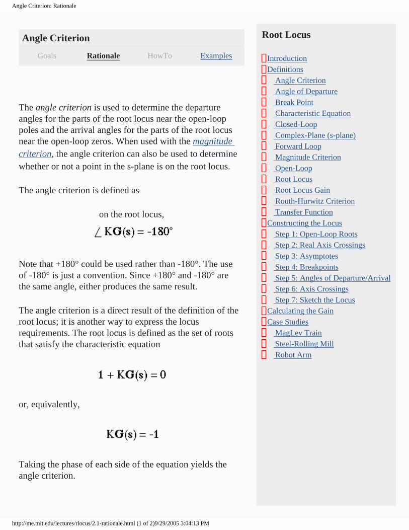
The angle criterion is used to determine the departure angles for the parts of the root locus near the open-loop poles and the arrival angles for the parts of the root locus near the open-loop zeros. When used with the magnitude criterion, the angle criterion can also be used to determine whether or not a point in the s-plane is on the root locus.
The angle criterion is defined as
on the root locus,
Note that +180° could be used rather than -180°. The use of -180° is just a convention. Since +180° and -180° are the same angle, either produces the same result.
The angle criterion is a direct result of the definition of the root locus; it is another way to express the locus requirements. The root locus is defined as the set of roots that satisfy the characteristic equation
or, equivalently,
Taking the phase of each side of the equation yields the angle criterion.
Root Locus
IntroductionDefinitions Angle Criterion Angle of Departure Break Point Characteristic Equation Closed-Loop Complex-Plane (s-plane) Forward Loop Magnitude Criterion Open-Loop Root Locus Root Locus Gain Routh-Hurwitz Criterion Transfer FunctionConstructing the Locus Step 1: Open-Loop Roots Step 2: Real Axis Crossings Step 3: Asymptotes Step 4: Breakpoints Step 5: Angles of Departure/Arrival Step 6: Axis Crossings Step 7: Sketch the LocusCalculating the GainCase Studies MagLev Train Steel-Rolling Mill Robot Arm
http://me.mit.edu/lectures/rlocus/2.1-rationale.html (1 of 2)9/29/2005 3:04:13 PM

Magnitude Criterion: Rationale
Magnitude Criterion
Goals Rationale HowTo Examples
The magnitude criterion is used to determine the locations of a set of roots in the s-plane for a given value of K.
Mathematically, the magnitude criterion is
The magnitude criterion is a direct result of the definition of the root locus; it is another way to express the locus requirements. The root locus is defined as the set of roots that satisfy the characteristic equation
or, equivalently,
Taking the magnitude of each side of the equation yields the magnitude criterion.
Root Locus
IntroductionDefinitions Angle Criterion Angle of Departure Break Point Characteristic Equation Closed-Loop Complex-Plane (s-plane) Forward Loop Magnitude Criterion Open-Loop Root Locus Root Locus Gain Routh-Hurwitz Criterion Transfer FunctionConstructing the Locus Step 1: Open-Loop Roots Step 2: Real Axis Crossings Step 3: Asymptotes Step 4: Breakpoints Step 5: Angles of Departure/Arrival Step 6: Axis Crossings Step 7: Sketch the LocusCalculating the GainCase Studies MagLev Train Steel-Rolling Mill Robot Arm
http://me.mit.edu/lectures/rlocus/2.8-rationale.html (1 of 2)9/29/2005 3:04:43 PM

Angle of Departure: Rationale
Angle of Departure
Goals Rationale HowTo Examples
The angle of departure is the angle at which the locus leaves a pole in the s-plane. The angle of arrival is the angle at which the locus arrives at a zero in the s-plane.
By convention, both types of angles are measured relative to a ray starting at the origin and extending to the right along the real axis in the s-plane.
Both arrival and departure angles are found using the angle criterion.
Root Locus
IntroductionDefinitions Angle Criterion Angle of Departure Break Point Characteristic Equation Closed-Loop Complex-Plane (s-plane) Forward Loop Magnitude Criterion Open-Loop Root Locus Root Locus Gain Routh-Hurwitz Criterion Transfer FunctionConstructing the Locus Step 1: Open-Loop Roots Step 2: Real Axis Crossings Step 3: Asymptotes Step 4: Breakpoints Step 5: Angles of Departure/Arrival Step 6: Axis Crossings Step 7: Sketch the LocusCalculating the GainCase Studies MagLev Train Steel-Rolling Mill Robot Arm
http://me.mit.edu/lectures/rlocus/2.2-rationale.html (1 of 2)9/29/2005 3:05:11 PM

Angle of Departure: Rationale
http://me.mit.edu/lectures/rlocus/2.2-rationale.html (2 of 2)9/29/2005 3:05:11 PM
Break Point: Rationale
Break Point
Goals Rationale HowTo Examples
Break points occur on the locus where two or more loci converge or diverge. Break points often occur on the real axis, but they may appear anywhere in the s-plane.
The loci that approach/diverge from a break point do so at angles spaced equally about the break point. The angles at which they arrive/leave are a function of the number of loci that approach/diverge from the break point.
Root Locus
IntroductionDefinitions Angle Criterion Angle of Departure Break Point Characteristic Equation Closed-Loop Complex-Plane (s-plane) Forward Loop Magnitude Criterion Open-Loop Root Locus Root Locus Gain Routh-Hurwitz Criterion Transfer FunctionConstructing the Locus Step 1: Open-Loop Roots Step 2: Real Axis Crossings Step 3: Asymptotes Step 4: Breakpoints Step 5: Angles of Departure/Arrival Step 6: Axis Crossings Step 7: Sketch the LocusCalculating the GainCase Studies MagLev Train Steel-Rolling Mill Robot Arm
http://me.mit.edu/lectures/rlocus/2.3-rationale.html (1 of 2)9/29/2005 3:05:33 PM

Break Point: Rationale
http://me.mit.edu/lectures/rlocus/2.3-rationale.html (2 of 2)9/29/2005 3:05:33 PM

Closed-Loop: Rationale
Closed-Loop
Goals Rationale HowTo Examples
A closed-loop system includes feedback. The output from the system is fed back through a controller into the input to the system. If Gu(s) is the transfer function of the
uncontrolled system, and Gc(s) is the transfer function of
the controller, and a unity feedback is used, then the closed-loop system can be represented in block diagram form as
Sometimes a transfer function, H(s), is included in the feedback loop. In block diagram form, this can be represented as
Root Locus
IntroductionDefinitions Angle Criterion Angle of Departure Break Point Characteristic Equation Closed-Loop Complex-Plane (s-plane) Forward Loop Magnitude Criterion Open-Loop Root Locus Root Locus Gain Routh-Hurwitz Criterion Transfer FunctionConstructing the Locus Step 1: Open-Loop Roots Step 2: Real Axis Crossings Step 3: Asymptotes Step 4: Breakpoints Step 5: Angles of Departure/Arrival Step 6: Axis Crossings Step 7: Sketch the LocusCalculating the GainCase Studies MagLev Train Steel-Rolling Mill Robot Arm
http://me.mit.edu/lectures/rlocus/2.5-rationale.html (1 of 2)9/29/2005 3:05:57 PM
Complex-Plane (s-plane): Rationale
Complex-Plane (s-plane)
Goals Rationale HowTo Examples
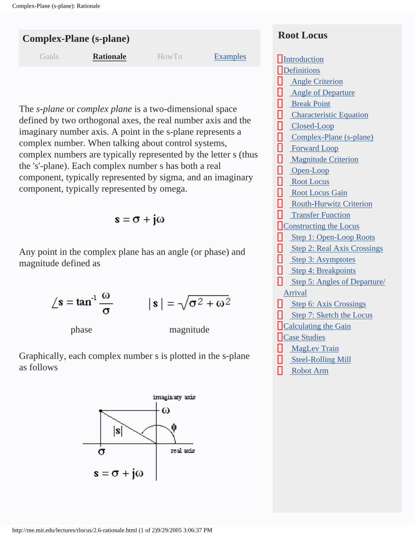
The s-plane or complex plane is a two-dimensional space defined by two orthogonal axes, the real number axis and the imaginary number axis. A point in the s-plane represents a complex number. When talking about control systems, complex numbers are typically represented by the letter s (thus the 's'-plane). Each complex number s has both a real component, typically represented by sigma, and an imaginary component, typically represented by omega.
Any point in the complex plane has an angle (or phase) and magnitude defined as
phase magnitude
Graphically, each complex number s is plotted in the s-plane as follows
Root Locus
IntroductionDefinitions Angle Criterion Angle of Departure Break Point Characteristic Equation Closed-Loop Complex-Plane (s-plane) Forward Loop Magnitude Criterion Open-Loop Root Locus Root Locus Gain Routh-Hurwitz Criterion Transfer FunctionConstructing the Locus Step 1: Open-Loop Roots Step 2: Real Axis Crossings Step 3: Asymptotes Step 4: Breakpoints Step 5: Angles of Departure/Arrival Step 6: Axis Crossings Step 7: Sketch the LocusCalculating the GainCase Studies MagLev Train Steel-Rolling Mill Robot Arm
http://me.mit.edu/lectures/rlocus/2.6-rationale.html (1 of 2)9/29/2005 3:06:37 PM
Forward Loop: Rationale
Forward Loop
Goals Rationale HowTo Examples
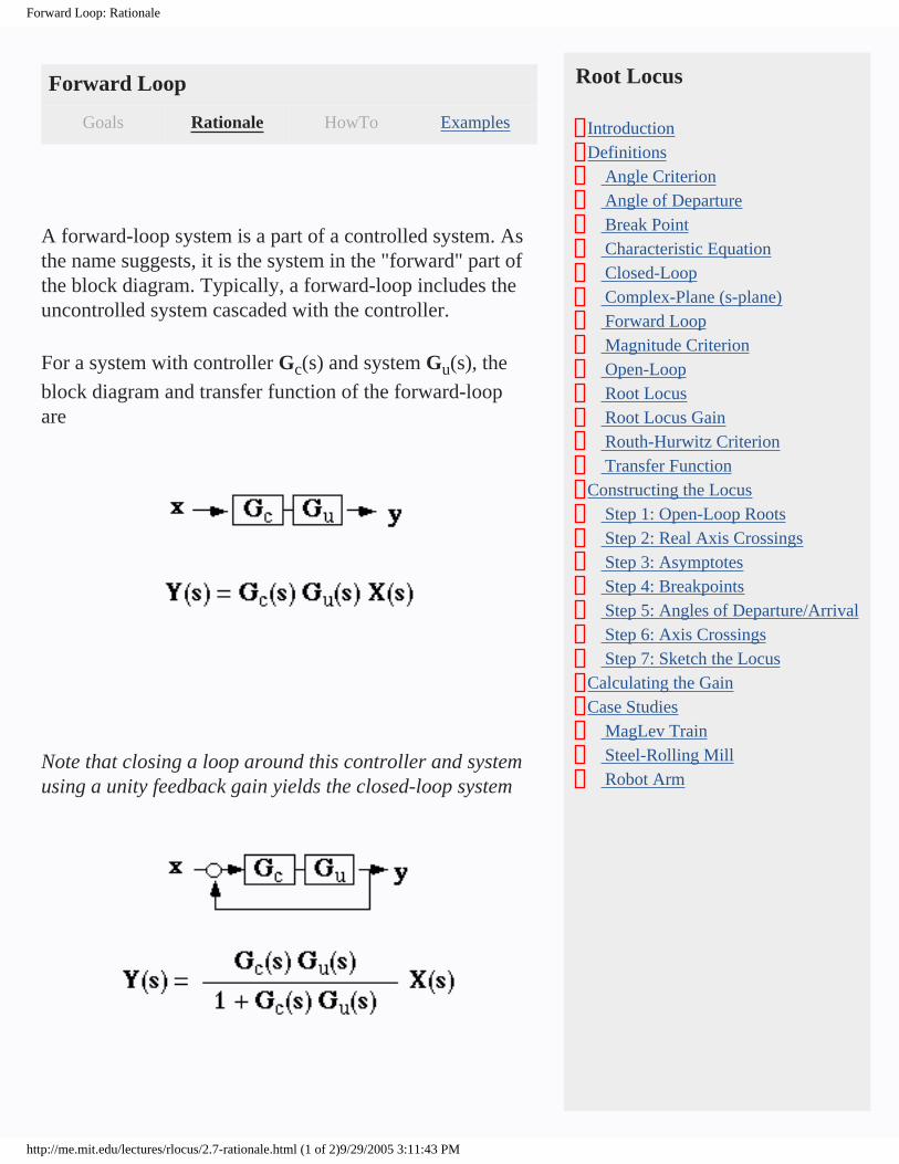
A forward-loop system is a part of a controlled system. As the name suggests, it is the system in the "forward" part of the block diagram. Typically, a forward-loop includes the uncontrolled system cascaded with the controller.
For a system with controller Gc(s) and system Gu(s), the
block diagram and transfer function of the forward-loop are
Note that closing a loop around this controller and system using a unity feedback gain yields the closed-loop system
Root Locus
IntroductionDefinitions Angle Criterion Angle of Departure Break Point Characteristic Equation Closed-Loop Complex-Plane (s-plane) Forward Loop Magnitude Criterion Open-Loop Root Locus Root Locus Gain Routh-Hurwitz Criterion Transfer FunctionConstructing the Locus Step 1: Open-Loop Roots Step 2: Real Axis Crossings Step 3: Asymptotes Step 4: Breakpoints Step 5: Angles of Departure/Arrival Step 6: Axis Crossings Step 7: Sketch the LocusCalculating the GainCase Studies MagLev Train Steel-Rolling Mill Robot Arm
http://me.mit.edu/lectures/rlocus/2.7-rationale.html (1 of 2)9/29/2005 3:11:43 PM

Forward Loop: Rationale
http://me.mit.edu/lectures/rlocus/2.7-rationale.html (2 of 2)9/29/2005 3:11:43 PM
Open-Loop: Rationale
Open-Loop
Goals Rationale HowTo Examples
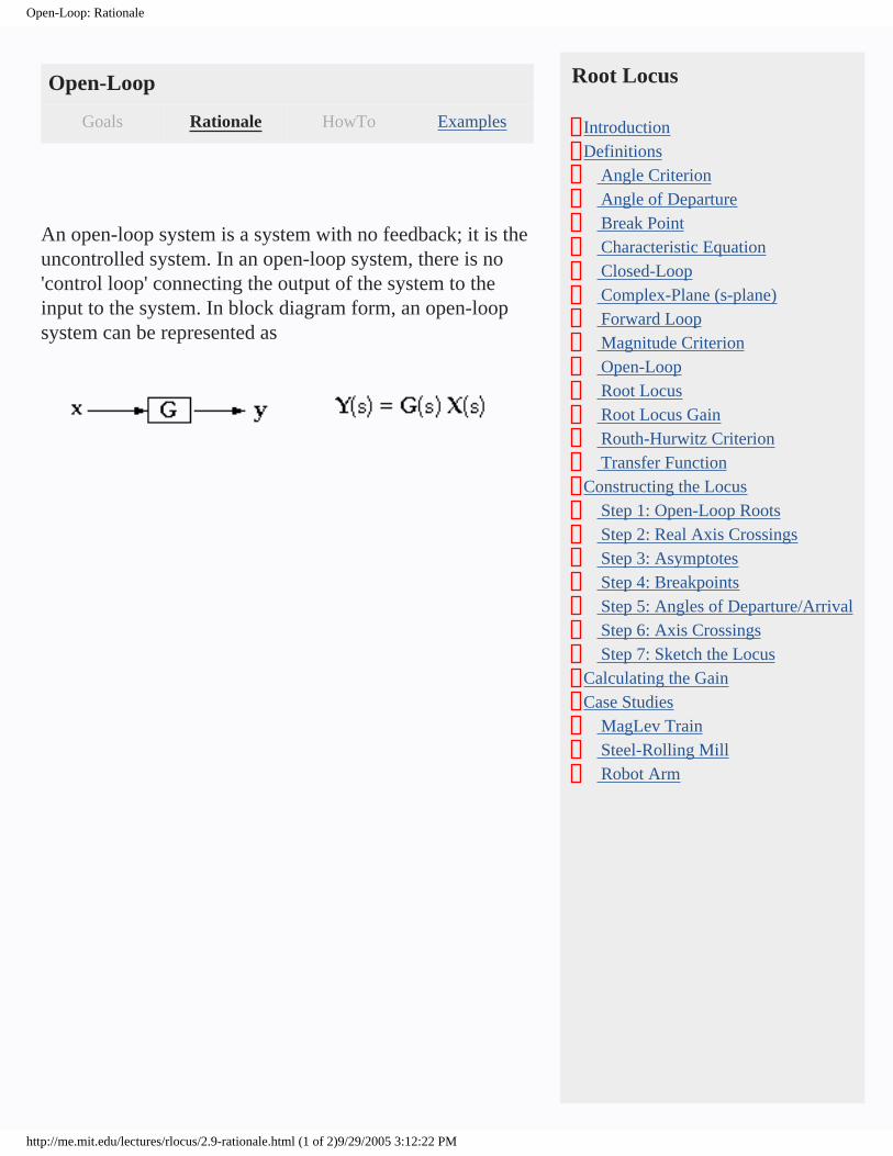
An open-loop system is a system with no feedback; it is the uncontrolled system. In an open-loop system, there is no 'control loop' connecting the output of the system to the input to the system. In block diagram form, an open-loop system can be represented as
Root Locus
IntroductionDefinitions Angle Criterion Angle of Departure Break Point Characteristic Equation Closed-Loop Complex-Plane (s-plane) Forward Loop Magnitude Criterion Open-Loop Root Locus Root Locus Gain Routh-Hurwitz Criterion Transfer FunctionConstructing the Locus Step 1: Open-Loop Roots Step 2: Real Axis Crossings Step 3: Asymptotes Step 4: Breakpoints Step 5: Angles of Departure/Arrival Step 6: Axis Crossings Step 7: Sketch the LocusCalculating the GainCase Studies MagLev Train Steel-Rolling Mill Robot Arm
http://me.mit.edu/lectures/rlocus/2.9-rationale.html (1 of 2)9/29/2005 3:12:22 PM

Open-Loop: Rationale
http://me.mit.edu/lectures/rlocus/2.9-rationale.html (2 of 2)9/29/2005 3:12:22 PM

Routh-Hurwitz Criterion: Rationale
Routh-Hurwitz Criterion
Goals Rationale HowTo Examples
The Routh-Hurwitz stability criterion is a method for determining whether or not a system is stable based upon the coefficients in the system's characteristic equation. It is particularly useful for higher-order systems because it does not require the polynomial expressions in the transfer function to be factored.
Root Locus
IntroductionDefinitions Angle Criterion Angle of Departure Break Point Characteristic Equation Closed-Loop Complex-Plane (s-plane) Forward Loop Magnitude Criterion Open-Loop Root Locus Root Locus Gain Routh-Hurwitz Criterion Transfer FunctionConstructing the Locus Step 1: Open-Loop Roots Step 2: Real Axis Crossings Step 3: Asymptotes Step 4: Breakpoints Step 5: Angles of Departure/Arrival Step 6: Axis Crossings Step 7: Sketch the LocusCalculating the GainCase Studies MagLev Train Steel-Rolling Mill Robot Arm
http://me.mit.edu/lectures/rlocus/2.12-rationale.html (1 of 2)9/29/2005 3:14:16 PM

Transfer Function: Rationale
Transfer Function
Goals Rationale HowTo Examples
A transfer function defines the relationship between the inputs to a system and its outputs. The transfer function is typically written in the frequency, or 's' domain, rather than the time domain. The LaPlace transform is used to map the time domain representation into the frequency domain representation.
If x(t) is the input to the system and y(t) is the output from the system, and the LaPlace transform of the input is X(s) and the LaPlace transform of the output is Y(s), then the transfer function between the input and the output is
Y(s)----X(s)
Root Locus
IntroductionDefinitions Angle Criterion Angle of Departure Break Point Characteristic Equation Closed-Loop Complex-Plane (s-plane) Forward Loop Magnitude Criterion Open-Loop Root Locus Root Locus Gain Routh-Hurwitz Criterion Transfer FunctionConstructing the Locus Step 1: Open-Loop Roots Step 2: Real Axis Crossings Step 3: Asymptotes Step 4: Breakpoints Step 5: Angles of Departure/Arrival Step 6: Axis Crossings Step 7: Sketch the LocusCalculating the GainCase Studies MagLev Train Steel-Rolling Mill Robot Arm
http://me.mit.edu/lectures/rlocus/2.13-rationale.html (1 of 2)9/29/2005 3:15:13 PM

Constructing the Locus: Goals
Constructing the Locus
Goals Rationale HowTo Examples
This section outlines the steps to creating a root locus and illustrates the important properties of each step in the process. By the end of this section you should be able to sketch a root locus given the forward-loop poles and zeros of a system. Using these steps, the locus will be detailed enough to evaluate the stability and robustness properties of the closed-loop controller.
Root Locus
IntroductionDefinitions Angle Criterion Angle of Departure Break Point Characteristic Equation Closed-Loop Complex-Plane (s-plane) Forward Loop Magnitude Criterion Open-Loop Root Locus Root Locus Gain Routh-Hurwitz Criterion Transfer FunctionConstructing the Locus Step 1: Open-Loop Roots Step 2: Real Axis Crossings Step 3: Asymptotes Step 4: Breakpoints Step 5: Angles of Departure/Arrival Step 6: Axis Crossings Step 7: Sketch the LocusCalculating the GainCase Studies MagLev Train Steel-Rolling Mill Robot Arm
http://me.mit.edu/lectures/rlocus/3-goals.html (1 of 2)9/29/2005 3:33:52 PM

Constructing the Locus: Goals
http://me.mit.edu/lectures/rlocus/3-goals.html (2 of 2)9/29/2005 3:33:52 PM

Step 1: Open-Loop Roots: Rationale
Step 1: Open-Loop Roots
Goals Rationale HowTo Examples
Start with the forward-loop poles and zeros. Since the locus represents the path of the roots (specifically, paths of the closed-loop poles) as the root locus gain is varied, we start with the forward-loop configuration, i.e. the location of the roots when the gain of the closed-loop system is 0. Each locus starts at a forward-loop pole and ends at a forward-loop zero. If the system has more poles than zeros, then some of the loci end at zeros located infinitely far from the poles.
Root Locus
IntroductionDefinitions Angle Criterion Angle of Departure Break Point Characteristic Equation Closed-Loop Complex-Plane (s-plane) Forward Loop Magnitude Criterion Open-Loop Root Locus Root Locus Gain Routh-Hurwitz Criterion Transfer FunctionConstructing the Locus Step 1: Open-Loop Roots Step 2: Real Axis Crossings Step 3: Asymptotes Step 4: Breakpoints Step 5: Angles of Departure/Arrival Step 6: Axis Crossings Step 7: Sketch the LocusCalculating the GainCase Studies MagLev Train Steel-Rolling Mill Robot Arm
http://me.mit.edu/lectures/rlocus/3.1-rationale.html (1 of 2)9/29/2005 3:37:20 PM

Step 2: Real Axis Crossings: Rationale
Step 2: Real Axis Crossings
Goals Rationale HowTo Examples
Many root loci have paths on the real axis. The real axis portion of the locus is determined by applying the following rule:
If an odd number of forward-loop poles and forward-loop zeros lie to the right of a point on the real axis, that point belongs to the root locus.
Note that the real axis section of the root locus is determined entirely by the number of forward-loop poles and zeros and their relative locations.
Since the final root locus is always symmetric about the real axis (think about it), the real axis part is pretty easy to do.
Root Locus
IntroductionDefinitions Angle Criterion Angle of Departure Break Point Characteristic Equation Closed-Loop Complex-Plane (s-plane) Forward Loop Magnitude Criterion Open-Loop Root Locus Root Locus Gain Routh-Hurwitz Criterion Transfer FunctionConstructing the Locus Step 1: Open-Loop Roots Step 2: Real Axis Crossings Step 3: Asymptotes Step 4: Breakpoints Step 5: Angles of Departure/Arrival Step 6: Axis Crossings Step 7: Sketch the LocusCalculating the GainCase Studies MagLev Train Steel-Rolling Mill Robot Arm
http://me.mit.edu/lectures/rlocus/3.2-rationale.html (1 of 2)9/29/2005 3:39:32 PM
Step 3: Asymptotes: Rationale
Step 3: Asymptotes
Goals Rationale HowTo Examples
The asymptotes indicate where the poles will go as the gain approaches infinity. For systems with more poles than zeros, the number of asymptotes is equal to the number of poles minus the number of zeros. In some systems, there are no asymptotes; when the number of poles is equal to the number of zeros then each locus is terminated at a zero rather than asymptotically to infinity.
The asymptotes are symmetric about the real axis, and they stem from a point defined by the relative magnitudes of the open-loop roots. This point is called the centroid.
Note that it is possible to draw a root locus for systems with more zeros than poles, but such systems do not represent physical systems. In these cases, you can think of some of the poles being located at infinity.
Root Locus
IntroductionDefinitions Angle Criterion Angle of Departure Break Point Characteristic Equation Closed-Loop Complex-Plane (s-plane) Forward Loop Magnitude Criterion Open-Loop Root Locus Root Locus Gain Routh-Hurwitz Criterion Transfer FunctionConstructing the Locus Step 1: Open-Loop Roots Step 2: Real Axis Crossings Step 3: Asymptotes Step 4: Breakpoints Step 5: Angles of Departure/Arrival Step 6: Axis Crossings Step 7: Sketch the LocusCalculating the GainCase Studies MagLev Train Steel-Rolling Mill Robot Arm
http://me.mit.edu/lectures/rlocus/3.3-rationale.html (1 of 2)9/29/2005 3:39:53 PM
Step 4: Breakpoints: Rationale
Step 4: Breakpoints
Goals Rationale HowTo Examples
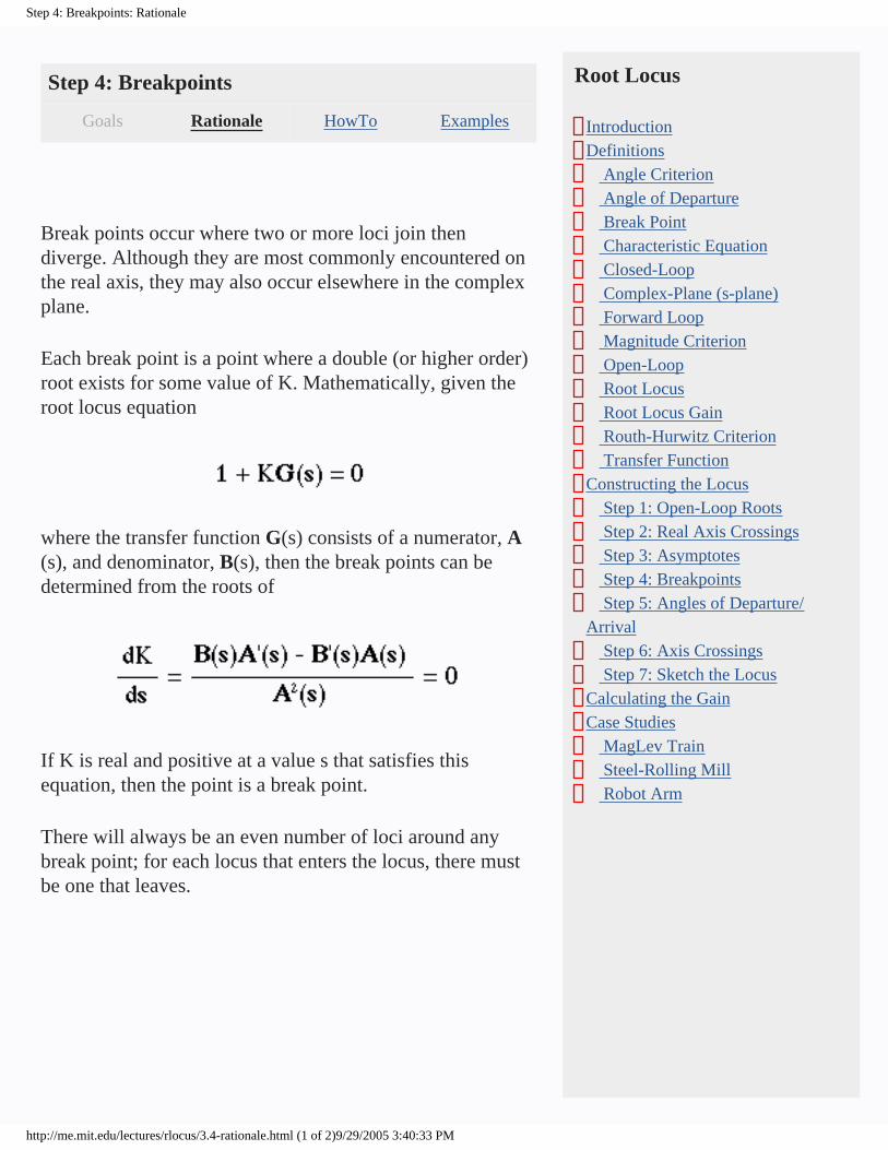
Break points occur where two or more loci join then diverge. Although they are most commonly encountered on the real axis, they may also occur elsewhere in the complex plane.
Each break point is a point where a double (or higher order) root exists for some value of K. Mathematically, given the root locus equation
where the transfer function G(s) consists of a numerator, A(s), and denominator, B(s), then the break points can be determined from the roots of
If K is real and positive at a value s that satisfies this equation, then the point is a break point.
There will always be an even number of loci around any break point; for each locus that enters the locus, there must be one that leaves.
Root Locus
IntroductionDefinitions Angle Criterion Angle of Departure Break Point Characteristic Equation Closed-Loop Complex-Plane (s-plane) Forward Loop Magnitude Criterion Open-Loop Root Locus Root Locus Gain Routh-Hurwitz Criterion Transfer FunctionConstructing the Locus Step 1: Open-Loop Roots Step 2: Real Axis Crossings Step 3: Asymptotes Step 4: Breakpoints Step 5: Angles of Departure/Arrival Step 6: Axis Crossings Step 7: Sketch the LocusCalculating the GainCase Studies MagLev Train Steel-Rolling Mill Robot Arm
http://me.mit.edu/lectures/rlocus/3.4-rationale.html (1 of 2)9/29/2005 3:40:33 PM

Step 5: Angles of Departure/Arrival: Rationale
Step 5: Angles of Departure/Arrival
Goals Rationale HowTo Examples
The angle criterion determines which direction the roots move as the gain moves from zero (angles of departure, at the forward-loop poles) to infinity (angles of arrival, at the forward-loop zeros).
An angle of departure/arrival is calculated at each of the complex forward-loop poles and zeros.
Root Locus
IntroductionDefinitions Angle Criterion Angle of Departure Break Point Characteristic Equation Closed-Loop Complex-Plane (s-plane) Forward Loop Magnitude Criterion Open-Loop Root Locus Root Locus Gain Routh-Hurwitz Criterion Transfer FunctionConstructing the Locus Step 1: Open-Loop Roots Step 2: Real Axis Crossings Step 3: Asymptotes Step 4: Breakpoints Step 5: Angles of Departure/Arrival Step 6: Axis Crossings Step 7: Sketch the LocusCalculating the GainCase Studies MagLev Train Steel-Rolling Mill Robot Arm
http://me.mit.edu/lectures/rlocus/3.5-rationale.html (1 of 2)9/29/2005 3:41:03 PM
Step 6: Axis Crossings: Rationale
Step 6: Axis Crossings
Goals Rationale HowTo Examples
The points where the root locus intersects the imaginary axis indicate the values of K at which the closed loop system is marginally stable. The closed loop system will be unstable for any gain for which the locus is in the right half-plane of the complex plane.
If the root locus crosses the imaginary axis from left to right at a point where K=K0 and then stays completely in
the right half-plane, then the closed-loop system is unstable for all K>K0. Therefore, knowing the value of K0 is very
useful.
Some systems are particularly nasty when their locus dips back and forth across the imaginary axis. In these systems, increasing the root locus gain will cause the system to go unstable initially and then becomes stable again.
Root Locus
IntroductionDefinitions Angle Criterion Angle of Departure Break Point Characteristic Equation Closed-Loop Complex-Plane (s-plane) Forward Loop Magnitude Criterion Open-Loop Root Locus Root Locus Gain Routh-Hurwitz Criterion Transfer FunctionConstructing the Locus Step 1: Open-Loop Roots Step 2: Real Axis Crossings Step 3: Asymptotes Step 4: Breakpoints Step 5: Angles of Departure/Arrival Step 6: Axis Crossings Step 7: Sketch the LocusCalculating the GainCase Studies MagLev Train Steel-Rolling Mill Robot Arm
http://me.mit.edu/lectures/rlocus/3.6-rationale.html (1 of 2)9/29/2005 3:41:41 PM

Step 7: Sketch the Locus: Rationale
Step 7: Sketch the Locus
Goals Rationale HowTo Examples
The complete root locus can be drawn by starting from the forward-loop poles, connecting the real axis section, break points, and axis crossings, then ending at either the forward-loop zeros or along the asymptotes to infinity and beyond.
If your hand-drawn locus is not detailed enough to determine the behavior of your system, then you may want to use Matlab or some other computer tool to calculate the locus exactly.
Root Locus
IntroductionDefinitions Angle Criterion Angle of Departure Break Point Characteristic Equation Closed-Loop Complex-Plane (s-plane) Forward Loop Magnitude Criterion Open-Loop Root Locus Root Locus Gain Routh-Hurwitz Criterion Transfer FunctionConstructing the Locus Step 1: Open-Loop Roots Step 2: Real Axis Crossings Step 3: Asymptotes Step 4: Breakpoints Step 5: Angles of Departure/Arrival Step 6: Axis Crossings Step 7: Sketch the LocusCalculating the GainCase Studies MagLev Train Steel-Rolling Mill Robot Arm
http://me.mit.edu/lectures/rlocus/3.7-rationale.html (1 of 2)9/29/2005 3:44:44 PM

Calculating the Gain: Goals
Calculating the Gain
Goals Rationale HowTo Examples
After reading this section you should be able to calculate the root locus gain at any point on the locus.
Root Locus
IntroductionDefinitions Angle Criterion Angle of Departure Break Point Characteristic Equation Closed-Loop Complex-Plane (s-plane) Forward Loop Magnitude Criterion Open-Loop Root Locus Root Locus Gain Routh-Hurwitz Criterion Transfer FunctionConstructing the Locus Step 1: Open-Loop Roots Step 2: Real Axis Crossings Step 3: Asymptotes Step 4: Breakpoints Step 5: Angles of Departure/Arrival Step 6: Axis Crossings Step 7: Sketch the LocusCalculating the GainCase Studies MagLev Train Steel-Rolling Mill Robot Arm
http://me.mit.edu/lectures/rlocus/4-goals.html (1 of 2)9/29/2005 3:46:35 PM

Calculating the Gain: Goals
http://me.mit.edu/lectures/rlocus/4-goals.html (2 of 2)9/29/2005 3:46:35 PM

Calculating the Gain: Rationale
Calculating the Gain
Goals Rationale HowTo Examples
The root locus shows you graphically how the system roots will move as you change the root locus gain. Often, however, one must determine the gain at critical points on the locus, such as points where the locus crosses the imaginary axis.
Root Locus
IntroductionDefinitions Angle Criterion Angle of Departure Break Point Characteristic Equation Closed-Loop Complex-Plane (s-plane) Forward Loop Magnitude Criterion Open-Loop Root Locus Root Locus Gain Routh-Hurwitz Criterion Transfer FunctionConstructing the Locus Step 1: Open-Loop Roots Step 2: Real Axis Crossings Step 3: Asymptotes Step 4: Breakpoints Step 5: Angles of Departure/Arrival Step 6: Axis Crossings Step 7: Sketch the LocusCalculating the GainCase Studies MagLev Train Steel-Rolling Mill Robot Arm
http://me.mit.edu/lectures/rlocus/4-rationale.html (1 of 2)9/29/2005 3:47:16 PM

Calculating the Gain: Rationale
http://me.mit.edu/lectures/rlocus/4-rationale.html (2 of 2)9/29/2005 3:47:16 PM

Calculating the Gain: HowTo
Calculating the Gain
Goals Rationale HowTo Examples
The magnitude criterion is used to determine the value of the root locus gain, K, at any point on the root locus.
The gain is calculated by multiplying the lengths of the distance between each pole to the point then dividing that by the product of the lengths of the distance between each zero and the point.
Root Locus
IntroductionDefinitions Angle Criterion Angle of Departure Break Point Characteristic Equation Closed-Loop Complex-Plane (s-plane) Forward Loop Magnitude Criterion Open-Loop Root Locus Root Locus Gain Routh-Hurwitz Criterion Transfer FunctionConstructing the Locus Step 1: Open-Loop Roots Step 2: Real Axis Crossings Step 3: Asymptotes Step 4: Breakpoints Step 5: Angles of Departure/Arrival Step 6: Axis Crossings Step 7: Sketch the LocusCalculating the GainCase Studies MagLev Train Steel-Rolling Mill Robot Arm
http://me.mit.edu/lectures/rlocus/4-howto.html (1 of 2)9/29/2005 3:47:38 PM

Calculating the Gain: HowTo
http://me.mit.edu/lectures/rlocus/4-howto.html (2 of 2)9/29/2005 3:47:38 PM

Calculating the Gain: Examples
Calculating the Gain
Goals Rationale HowTo Examples
Consider the system with transfer function
and corresponding root locus
The gain at the point (-1, 0) is thus
The root locus gain for other points on the locus are given in the following table:
coordinate gain
0.75,0 0.9375
0.5,0 1.75
0.25,0 2.4375
0,0 4
Root Locus
IntroductionDefinitions Angle Criterion Angle of Departure Break Point Characteristic Equation Closed-Loop Complex-Plane (s-plane) Forward Loop Magnitude Criterion Open-Loop Root Locus Root Locus Gain Routh-Hurwitz Criterion Transfer FunctionConstructing the Locus Step 1: Open-Loop Roots Step 2: Real Axis Crossings Step 3: Asymptotes Step 4: Breakpoints Step 5: Angles of Departure/Arrival Step 6: Axis Crossings Step 7: Sketch the LocusCalculating the GainCase Studies MagLev Train Steel-Rolling Mill Robot Arm
http://me.mit.edu/lectures/rlocus/4-examples.html (1 of 2)9/29/2005 3:48:09 PM

Calculating the Gain: Examples
0,0.25 4.0625
0,0.5 4.25
0,0.75 4.5625
0,1 5
0,2 8
0,3 13
Note that a linear change in position on the locus usually does not correspond to a linear change in the root locus gain.
http://me.mit.edu/lectures/rlocus/4-examples.html (2 of 2)9/29/2005 3:48:09 PM
Case Studies: Goals
Case Studies
Goals Rationale HowTo Examples
The case studies in this section should help you understand how to apply root locus principles to real problems.
As you may have noted, many systems look much different as a transfer function than they do as a real, physical system. The mapping from a controller transfer function to what actually happens to the system is also often not obvious.
This section should help you see the difference between open loop and closed loop behavior in real systems. In particular, the cases illustrate how changing the root locus gain affects the system behavior.
Root Locus
IntroductionDefinitions Angle Criterion Angle of Departure Break Point Characteristic Equation Closed-Loop Complex-Plane (s-plane) Forward Loop Magnitude Criterion Open-Loop Root Locus Root Locus Gain Routh-Hurwitz Criterion Transfer FunctionConstructing the Locus Step 1: Open-Loop Roots Step 2: Real Axis Crossings Step 3: Asymptotes Step 4: Breakpoints Step 5: Angles of Departure/Arrival Step 6: Axis Crossings Step 7: Sketch the LocusCalculating the GainCase Studies MagLev Train Steel-Rolling Mill Robot Arm
http://me.mit.edu/lectures/rlocus/5-goals.html (1 of 2)9/29/2005 3:48:36 PM

Case Studies: Goals
http://me.mit.edu/lectures/rlocus/5-goals.html (2 of 2)9/29/2005 3:48:36 PM

MagLev Train: Goals
MagLev Train
Goals Rationale HowTo Examples
After reading this case you should understand how root locus can be applied to inherently unstable systems in order to design a controller that will regulate the system despite its instability.
Root Locus
IntroductionDefinitions Angle Criterion Angle of Departure Break Point Characteristic Equation Closed-Loop Complex-Plane (s-plane) Forward Loop Magnitude Criterion Open-Loop Root Locus Root Locus Gain Routh-Hurwitz Criterion Transfer FunctionConstructing the Locus Step 1: Open-Loop Roots Step 2: Real Axis Crossings Step 3: Asymptotes Step 4: Breakpoints Step 5: Angles of Departure/Arrival Step 6: Axis Crossings Step 7: Sketch the LocusCalculating the GainCase Studies MagLev Train Steel-Rolling Mill Robot Arm
http://me.mit.edu/lectures/rlocus/5.1-goals.html (1 of 2)9/29/2005 3:49:13 PM

MagLev Train: Goals
http://me.mit.edu/lectures/rlocus/5.1-goals.html (2 of 2)9/29/2005 3:49:13 PM

Steel-Rolling Mill: Goals
Steel-Rolling Mill
Goals Rationale HowTo Examples
This case should help you understand how to use the root locus and feedback control as applied to relatively slow, stable processes.
Root Locus
IntroductionDefinitions Angle Criterion Angle of Departure Break Point Characteristic Equation Closed-Loop Complex-Plane (s-plane) Forward Loop Magnitude Criterion Open-Loop Root Locus Root Locus Gain Routh-Hurwitz Criterion Transfer FunctionConstructing the Locus Step 1: Open-Loop Roots Step 2: Real Axis Crossings Step 3: Asymptotes Step 4: Breakpoints Step 5: Angles of Departure/Arrival Step 6: Axis Crossings Step 7: Sketch the LocusCalculating the GainCase Studies MagLev Train Steel-Rolling Mill Robot Arm
http://me.mit.edu/lectures/rlocus/5.2-goals.html (1 of 2)9/29/2005 3:49:58 PM

Steel-Rolling Mill: Goals
http://me.mit.edu/lectures/rlocus/5.2-goals.html (2 of 2)9/29/2005 3:49:58 PM

Robot Arm: Goals
Robot Arm
Goals Rationale HowTo Examples
After reviewing this case you should understand how to use the root locus to design a controller for single degree of freedom robot arms.
Root Locus
IntroductionDefinitions Angle Criterion Angle of Departure Break Point Characteristic Equation Closed-Loop Complex-Plane (s-plane) Forward Loop Magnitude Criterion Open-Loop Root Locus Root Locus Gain Routh-Hurwitz Criterion Transfer FunctionConstructing the Locus Step 1: Open-Loop Roots Step 2: Real Axis Crossings Step 3: Asymptotes Step 4: Breakpoints Step 5: Angles of Departure/Arrival Step 6: Axis Crossings Step 7: Sketch the LocusCalculating the GainCase Studies MagLev Train Steel-Rolling Mill Robot Arm
http://me.mit.edu/lectures/rlocus/5.3-goals.html (1 of 2)9/29/2005 3:50:11 PM

Robot Arm: Goals
http://me.mit.edu/lectures/rlocus/5.3-goals.html (2 of 2)9/29/2005 3:50:11 PM
Robot Arm: Rationale
Robot Arm
Goals Rationale HowTo Examples
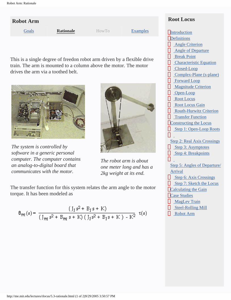
This is a single degree of freedon robot arm driven by a flexible drive train. The arm is mounted to a column above the motor. The motor drives the arm via a toothed belt.
The system is controlled by software in a generic personal computer. The computer contains an analog-to-digital board that communicates with the motor.
The robot arm is about one meter long and has a 2kg weight at its end.
The transfer function for this system relates the arm angle to the motor torque. It has been modeled as
Root Locus
IntroductionDefinitions Angle Criterion Angle of Departure Break Point Characteristic Equation Closed-Loop Complex-Plane (s-plane) Forward Loop Magnitude Criterion Open-Loop Root Locus Root Locus Gain Routh-Hurwitz Criterion Transfer FunctionConstructing the Locus Step 1: Open-Loop Roots Step 2: Real Axis Crossings Step 3: Asymptotes Step 4: Breakpoints Step 5: Angles of Departure/Arrival Step 6: Axis Crossings Step 7: Sketch the LocusCalculating the GainCase Studies MagLev Train Steel-Rolling Mill Robot Arm
http://me.mit.edu/lectures/rlocus/5.3-rationale.html (1 of 2)9/29/2005 3:50:57 PM

Robot Arm: Rationale
http://me.mit.edu/lectures/rlocus/5.3-rationale.html (2 of 2)9/29/2005 3:50:57 PM
Robot Arm: Examples
Robot Arm
Goals Rationale HowTo Examples
this section has not been completed - march 97
Root Locus
IntroductionDefinitions Angle Criterion Angle of Departure Break Point Characteristic Equation Closed-Loop Complex-Plane (s-plane) Forward Loop Magnitude Criterion Open-Loop Root Locus Root Locus Gain Routh-Hurwitz Criterion Transfer FunctionConstructing the Locus Step 1: Open-Loop Roots Step 2: Real Axis Crossings Step 3: Asymptotes Step 4: Breakpoints Step 5: Angles of Departure/Arrival Step 6: Axis Crossings Step 7: Sketch the LocusCalculating the GainCase Studies MagLev Train Steel-Rolling Mill Robot Arm
http://me.mit.edu/lectures/rlocus/5.3-examples.html (1 of 2)9/29/2005 3:51:23 PM

Robot Arm: Examples
http://me.mit.edu/lectures/rlocus/5.3-examples.html (2 of 2)9/29/2005 3:51:23 PM
Introduction: Rationale
Introduction
Goals Rationale HowTo Examples
Most control systems work by regulating the system they are controlling around a desired operating point. In practice, control systems must have the ability not only to regulate around an operating point, but also to reject disturbances and to be robust to changes in their environment.
The root locus method helps the designer of a control system to understand the stability and robustness properties of the controller at an operating point.
Root Locus
IntroductionDefinitions Angle Criterion Angle of Departure Break Point Characteristic Equation Closed-Loop Complex-Plane (s-plane) Forward Loop Magnitude Criterion Open-Loop Root Locus Root Locus Gain Routh-Hurwitz Criterion Transfer FunctionConstructing the Locus Step 1: Open-Loop Roots Step 2: Real Axis Crossings Step 3: Asymptotes Step 4: Breakpoints Step 5: Angles of Departure/Arrival Step 6: Axis Crossings Step 7: Sketch the LocusCalculating the GainCase Studies MagLev Train Steel-Rolling Mill Robot Arm
http://me.mit.edu/lectures/rlocus/1-rationale.html (1 of 2)9/29/2005 3:52:00 PM

Introduction: Rationale
http://me.mit.edu/lectures/rlocus/1-rationale.html (2 of 2)9/29/2005 3:52:00 PM

Introduction: Examples
Introduction
Goals Rationale HowTo Examples
Controllers are used in many different domains. This lecture includes case studies from various domains to illustrate the use of root locus. In each case, the controller is designed to regulate the system at some operating point, even when subjected to unexpected disturbances.
Here are examples of plants and their controllers in two different domains: transportation, process control, and position control. Each case is presented as an example of the use of feedback control.
Transportation - MagLev Trains
Magnetic levitation provides the mechanism for several new modes of transportation. Magnetically levitated trains, for example, provide a high speed, low friction, low noise alternative to conventional rail systems. The dynamics of magnetic levitation are inherently unstable, and thus require a controller to make the system behave in a useful manner.
Here the system is the mass of the train levitated by field-inducing coils. The input to the system is the current to the coils. The objective is to keep the train a safe distance above the coils. If the train is too high, it will leave the magnetic field and possibly veer to one side or the other. If the train is too low, it will touch the track with possibly disastrous results.
The response times in this system are fast, i.e. on the order of fractions of a second.
Root Locus
IntroductionDefinitions Angle Criterion Angle of Departure Break Point Characteristic Equation Closed-Loop Complex-Plane (s-plane) Forward Loop Magnitude Criterion Open-Loop Root Locus Root Locus Gain Routh-Hurwitz Criterion Transfer FunctionConstructing the Locus Step 1: Open-Loop Roots Step 2: Real Axis Crossings Step 3: Asymptotes Step 4: Breakpoints Step 5: Angles of Departure/Arrival Step 6: Axis Crossings Step 7: Sketch the LocusCalculating the GainCase Studies MagLev Train Steel-Rolling Mill Robot Arm
http://me.mit.edu/lectures/rlocus/1-examples.html (1 of 3)9/29/2005 3:52:30 PM

Introduction: Examples
Complete details about this case are in the MagLev Train Case Study section.
Process Control - Steel-Rolling Mill
Feedback control systems have been particularly successful in controlling manufacturing processes. Quantities such as temperature, flow, pressure, thickness, and chemical concentration are often precisely regulated in the presence of erratic behavior.
In a steel-rolling mill, slabs of red-hot steel are rolled into thin sheets. Some new mills do a continuous pour of steel into sheets, but in either case, the goal is to keep the sheet thickness uniform and accurate. In addition, periodically the thickness must be adjusted in order to fulfill orders for different thicknesses.
The response times in this system are relatively slow, i.e. on the order of minutes or even tens of minutes.
Complete details about this case are in the Steel-Rolling Mill Study section.
Position Control - Single DOF Manipulator
Feedback control is often used to drive a robot arm to a desired position. In this example, a single degree-of-freedom (DOF) arm is driven by an electric motor via a compliant belt.
The response times in this system are moderately fast, i.e. on the order of seconds.
Complete details about this case are in the Robot Arm Case
http://me.mit.edu/lectures/rlocus/1-examples.html (2 of 3)9/29/2005 3:52:30 PM

Introduction: Examples
Study section.
http://me.mit.edu/lectures/rlocus/1-examples.html (3 of 3)9/29/2005 3:52:30 PM

Steel-Rolling Mill: Rationale
Steel-Rolling Mill
Goals Rationale HowTo Examples
One of the remarkable successes of feedback control has occurred in process control. Quantities such as tempurature, flow, pressure, thickness, and chemical concentration, are often precisely regulated around their desired values using automatic control devices.
A specific example of process control is a high speed steelrolling mill where the goal is to keep the strip thickness accurate and readily adjustable. An automatic control system can be designed by incorporating a thickness sensor, a controller, and a motor. The objective is to design the controller using the root locus technique.
As in any control design procedure, the first step is to model the dynamics of the process, the actuator, and the sensor. The block diagram illustrating the model for this system is shown below.
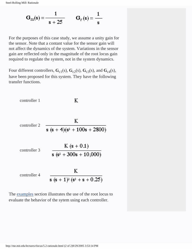
The motor and rollers have been modeled with the transfer functions Gm(s) and Gr(s), respectively.
Root Locus
IntroductionDefinitions Angle Criterion Angle of Departure Break Point Characteristic Equation Closed-Loop Complex-Plane (s-plane) Forward Loop Magnitude Criterion Open-Loop Root Locus Root Locus Gain Routh-Hurwitz Criterion Transfer FunctionConstructing the Locus Step 1: Open-Loop Roots Step 2: Real Axis Crossings Step 3: Asymptotes Step 4: Breakpoints Step 5: Angles of Departure/Arrival Step 6: Axis Crossings Step 7: Sketch the LocusCalculating the GainCase Studies MagLev Train Steel-Rolling Mill Robot Arm
http://me.mit.edu/lectures/rlocus/5.2-rationale.html (1 of 2)9/29/2005 3:53:14 PM
Steel-Rolling Mill: Rationale
For the purposes of this case study, we assume a unity gain for the sensor. Note that a contant value for the sensor gain will not affect the dynamics of the system. Variations in the sensor gain are reflected only in the magnitude of the root locus gain required to regulate the system, not in the system dynamics.
Four different controllers, Gc1(s), Gc2(s), Gc3(s), and Gc4(s),
have been proposed for this system. They have the following transfer functions.
controller 1
controller 2
controller 3
controller 4
The examples section illustrates the use of the root locus to evaluate the behavior of the sytem using each controller.
http://me.mit.edu/lectures/rlocus/5.2-rationale.html (2 of 2)9/29/2005 3:53:14 PM

Angle Criterion: Examples
Angle Criterion
Goals Rationale HowTo Examples
Given the system with forward-loop transfer function
and root locus
the phase angle for various points in the complex plane are listed in the following tables. The points in table 1 have a phase equal to 180 degrees and thus satisfy the angle criterion. Those in table 2 do not satisfy the angle criterion, and thus must not be on the root locus.
table 1 table 2
coordinate phase coordinate phase
0,0 180 -4,0 0
-1,1 180 -2,-2 150.3
-2,0 180 1,1 104
-1,-1 180 0,-1 206.6
Root Locus
IntroductionDefinitions Angle Criterion Angle of Departure Break Point Characteristic Equation Closed-Loop Complex-Plane (s-plane) Forward Loop Magnitude Criterion Open-Loop Root Locus Root Locus Gain Routh-Hurwitz Criterion Transfer FunctionConstructing the Locus Step 1: Open-Loop Roots Step 2: Real Axis Crossings Step 3: Asymptotes Step 4: Breakpoints Step 5: Angles of Departure/Arrival Step 6: Axis Crossings Step 7: Sketch the LocusCalculating the GainCase Studies MagLev Train Steel-Rolling Mill Robot Arm
http://me.mit.edu/lectures/rlocus/2.1-examples.html (1 of 2)9/29/2005 3:54:28 PM

Angle Criterion: Examples
http://me.mit.edu/lectures/rlocus/2.1-examples.html (2 of 2)9/29/2005 3:54:28 PM

Angle of Departure: Examples
Angle of Departure
Goals Rationale HowTo Examples
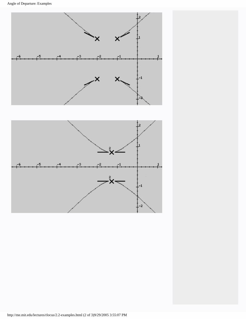
In the following images, the angles are indicated by the bold, short lines near the poles and zeros.
Root Locus
IntroductionDefinitions Angle Criterion Angle of Departure Break Point Characteristic Equation Closed-Loop Complex-Plane (s-plane) Forward Loop Magnitude Criterion Open-Loop Root Locus Root Locus Gain Routh-Hurwitz Criterion Transfer FunctionConstructing the Locus Step 1: Open-Loop Roots Step 2: Real Axis Crossings Step 3: Asymptotes Step 4: Breakpoints Step 5: Angles of Departure/Arrival Step 6: Axis Crossings Step 7: Sketch the LocusCalculating the GainCase Studies MagLev Train Steel-Rolling Mill Robot Arm
http://me.mit.edu/lectures/rlocus/2.2-examples.html (1 of 3)9/29/2005 3:55:07 PM
Angle of Departure: Examples
http://me.mit.edu/lectures/rlocus/2.2-examples.html (2 of 3)9/29/2005 3:55:07 PM

Angle of Departure: Examples
When there are multiple poles or zeros at a point in the complex plane, the angles are evenly distributed about the point.
http://me.mit.edu/lectures/rlocus/2.2-examples.html (3 of 3)9/29/2005 3:55:07 PM
Break Point: Examples
Break Point
Goals Rationale HowTo Examples
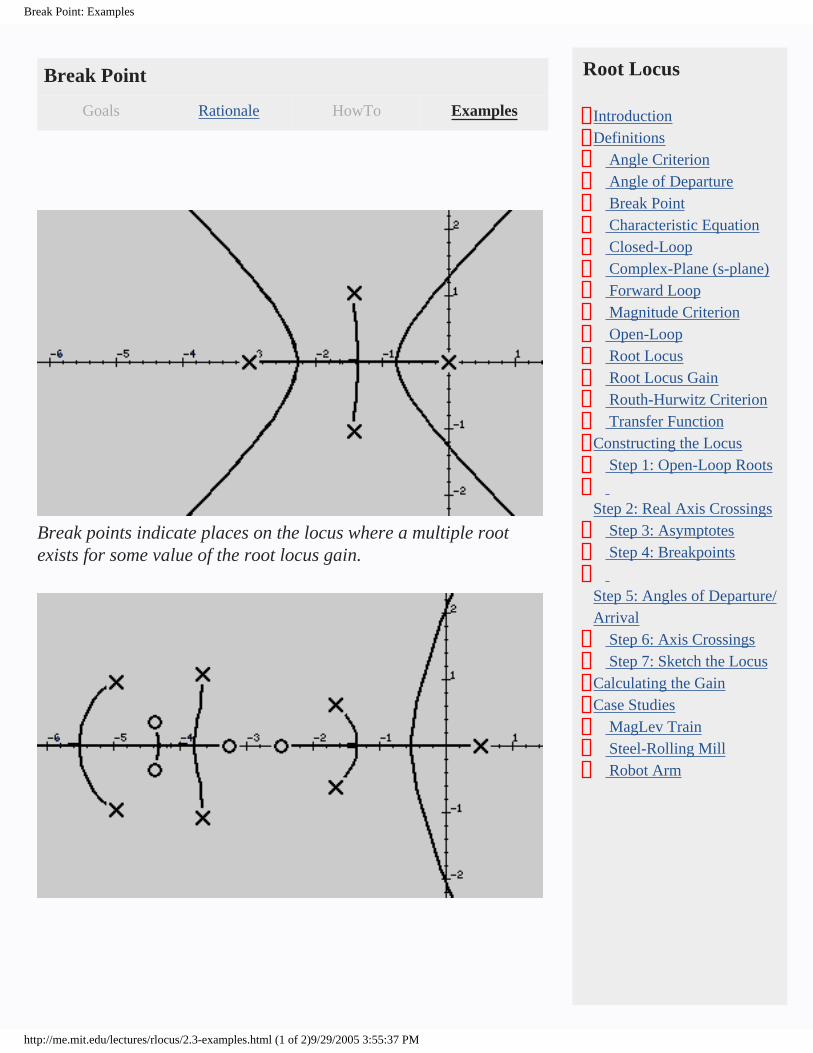
Break points indicate places on the locus where a multiple root exists for some value of the root locus gain.
Root Locus
IntroductionDefinitions Angle Criterion Angle of Departure Break Point Characteristic Equation Closed-Loop Complex-Plane (s-plane) Forward Loop Magnitude Criterion Open-Loop Root Locus Root Locus Gain Routh-Hurwitz Criterion Transfer FunctionConstructing the Locus Step 1: Open-Loop Roots Step 2: Real Axis Crossings Step 3: Asymptotes Step 4: Breakpoints Step 5: Angles of Departure/Arrival Step 6: Axis Crossings Step 7: Sketch the LocusCalculating the GainCase Studies MagLev Train Steel-Rolling Mill Robot Arm
http://me.mit.edu/lectures/rlocus/2.3-examples.html (1 of 2)9/29/2005 3:55:37 PM

Break Point: Examples
A break point may have more than to loci leading to/from it. In these cases, the break point indicates a point where a third- or higher-order root exists for some value of K.
Break points are most commonly encountered on the real axis, however they can occur anywhere in the complex plane.
http://me.mit.edu/lectures/rlocus/2.3-examples.html (2 of 2)9/29/2005 3:55:37 PM
Characteristic Equation: HowTo
Characteristic Equation
Goals Rationale HowTo Examples
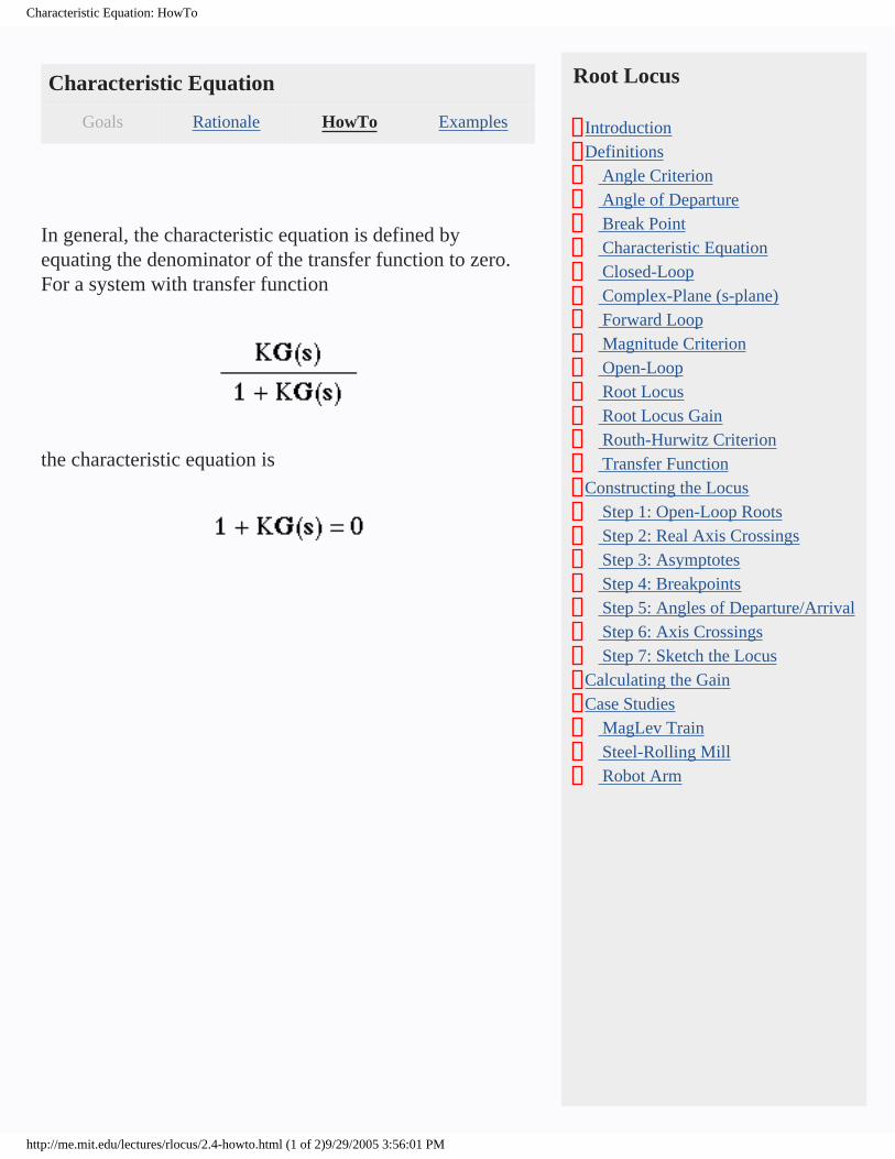
In general, the characteristic equation is defined by equating the denominator of the transfer function to zero. For a system with transfer function
the characteristic equation is
Root Locus
IntroductionDefinitions Angle Criterion Angle of Departure Break Point Characteristic Equation Closed-Loop Complex-Plane (s-plane) Forward Loop Magnitude Criterion Open-Loop Root Locus Root Locus Gain Routh-Hurwitz Criterion Transfer FunctionConstructing the Locus Step 1: Open-Loop Roots Step 2: Real Axis Crossings Step 3: Asymptotes Step 4: Breakpoints Step 5: Angles of Departure/Arrival Step 6: Axis Crossings Step 7: Sketch the LocusCalculating the GainCase Studies MagLev Train Steel-Rolling Mill Robot Arm
http://me.mit.edu/lectures/rlocus/2.4-howto.html (1 of 2)9/29/2005 3:56:01 PM

Characteristic Equation: HowTo
http://me.mit.edu/lectures/rlocus/2.4-howto.html (2 of 2)9/29/2005 3:56:01 PM

Characteristic Equation: Examples
Characteristic Equation
Goals Rationale HowTo Examples
Given a system with the transfer function
the characteristic equation is
Root Locus
IntroductionDefinitions Angle Criterion Angle of Departure Break Point Characteristic Equation Closed-Loop Complex-Plane (s-plane) Forward Loop Magnitude Criterion Open-Loop Root Locus Root Locus Gain Routh-Hurwitz Criterion Transfer FunctionConstructing the Locus Step 1: Open-Loop Roots Step 2: Real Axis Crossings Step 3: Asymptotes Step 4: Breakpoints Step 5: Angles of Departure/Arrival Step 6: Axis Crossings Step 7: Sketch the LocusCalculating the GainCase Studies MagLev Train Steel-Rolling Mill Robot Arm
http://me.mit.edu/lectures/rlocus/2.4-examples.html (1 of 2)9/29/2005 3:56:23 PM

Characteristic Equation: Examples
http://me.mit.edu/lectures/rlocus/2.4-examples.html (2 of 2)9/29/2005 3:56:23 PM

Closed-Loop: Examples
Closed-Loop
Goals Rationale HowTo Examples
Magnetically Levitated Train
From the maglev train case, the system, Gu(s), and a simple
controller, Gc(s), are defined as
The closed-loop transfer function is thus
Steel Rolling Mill
From the steel rolling case, the system, Gu(s), and a simple
controller, Gc(s), are defined as
The closed-loop transfer function is thus
Root Locus
IntroductionDefinitions Angle Criterion Angle of Departure Break Point Characteristic Equation Closed-Loop Complex-Plane (s-plane) Forward Loop Magnitude Criterion Open-Loop Root Locus Root Locus Gain Routh-Hurwitz Criterion Transfer FunctionConstructing the Locus Step 1: Open-Loop Roots Step 2: Real Axis Crossings Step 3: Asymptotes Step 4: Breakpoints Step 5: Angles of Departure/Arrival Step 6: Axis Crossings Step 7: Sketch the LocusCalculating the GainCase Studies MagLev Train Steel-Rolling Mill Robot Arm
http://me.mit.edu/lectures/rlocus/2.5-examples.html (1 of 2)9/29/2005 3:57:19 PM

Closed-Loop: Examples
http://me.mit.edu/lectures/rlocus/2.5-examples.html (2 of 2)9/29/2005 3:57:19 PM
Root Locus: HowTo
Root Locus
Goals Rationale HowTo Examples
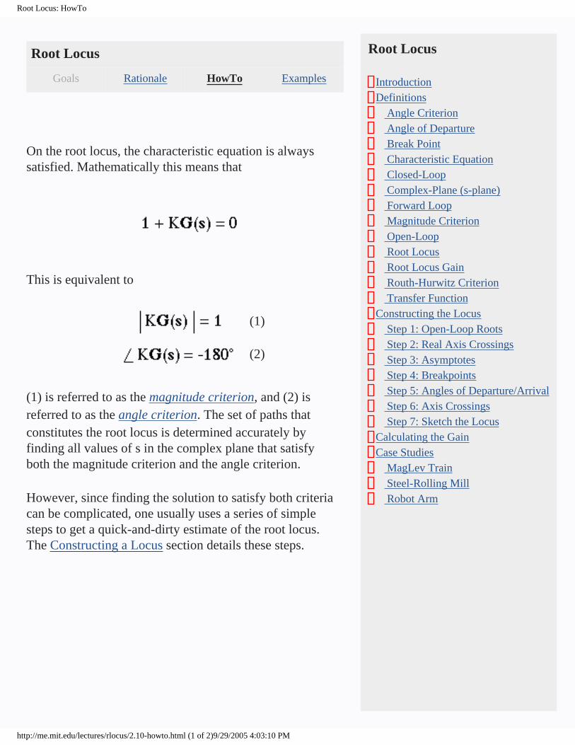
On the root locus, the characteristic equation is always satisfied. Mathematically this means that
This is equivalent to
(1)
(2)
(1) is referred to as the magnitude criterion, and (2) is referred to as the angle criterion. The set of paths that constitutes the root locus is determined accurately by finding all values of s in the complex plane that satisfy both the magnitude criterion and the angle criterion.
However, since finding the solution to satisfy both criteria can be complicated, one usually uses a series of simple steps to get a quick-and-dirty estimate of the root locus. The Constructing a Locus section details these steps.
Root Locus
IntroductionDefinitions Angle Criterion Angle of Departure Break Point Characteristic Equation Closed-Loop Complex-Plane (s-plane) Forward Loop Magnitude Criterion Open-Loop Root Locus Root Locus Gain Routh-Hurwitz Criterion Transfer FunctionConstructing the Locus Step 1: Open-Loop Roots Step 2: Real Axis Crossings Step 3: Asymptotes Step 4: Breakpoints Step 5: Angles of Departure/Arrival Step 6: Axis Crossings Step 7: Sketch the LocusCalculating the GainCase Studies MagLev Train Steel-Rolling Mill Robot Arm
http://me.mit.edu/lectures/rlocus/2.10-howto.html (1 of 2)9/29/2005 4:03:10 PM

Root Locus: HowTo
http://me.mit.edu/lectures/rlocus/2.10-howto.html (2 of 2)9/29/2005 4:03:10 PM

Root Locus: Examples
Root Locus
Goals Rationale HowTo Examples
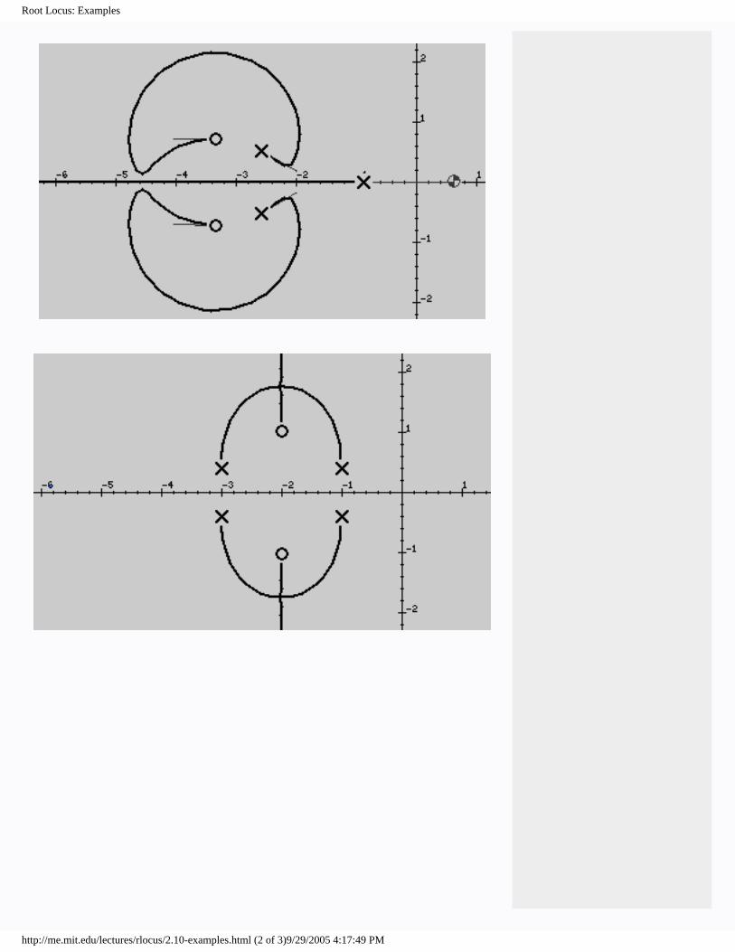
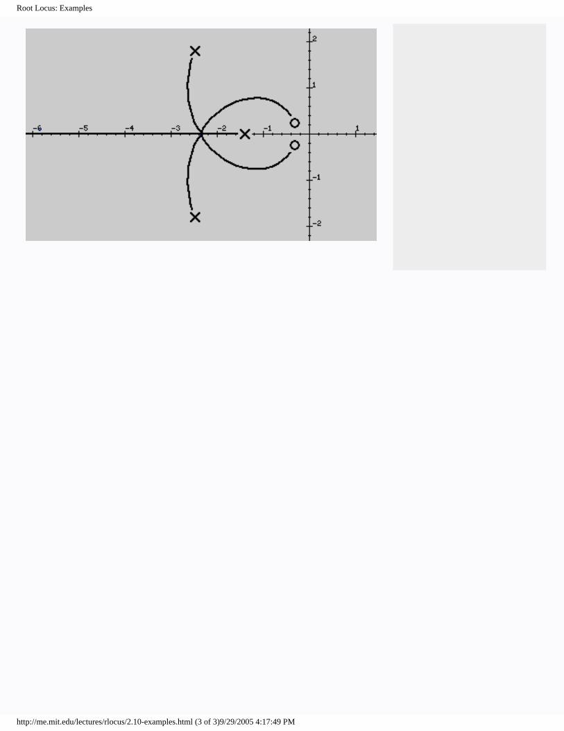
These are examples of typical (and not-so-typical) root loci.
magnetically levitated train
steel rolling locus
steel rolling mill
Root Locus
IntroductionDefinitions Angle Criterion Angle of Departure Break Point Characteristic Equation Closed-Loop Complex-Plane (s-plane) Forward Loop Magnitude Criterion Open-Loop Root Locus Root Locus Gain Routh-Hurwitz Criterion Transfer FunctionConstructing the Locus Step 1: Open-Loop Roots Step 2: Real Axis Crossings Step 3: Asymptotes Step 4: Breakpoints Step 5: Angles of Departure/Arrival Step 6: Axis Crossings Step 7: Sketch the LocusCalculating the GainCase Studies MagLev Train Steel-Rolling Mill Robot Arm
http://me.mit.edu/lectures/rlocus/2.10-examples.html (1 of 3)9/29/2005 4:17:49 PM
Root Locus: Examples
http://me.mit.edu/lectures/rlocus/2.10-examples.html (2 of 3)9/29/2005 4:17:49 PM
Root Locus: Examples
http://me.mit.edu/lectures/rlocus/2.10-examples.html (3 of 3)9/29/2005 4:17:49 PM

Open-Loop: Examples
Open-Loop
Goals Rationale HowTo Examples
Magnetically Levitated Train
From the maglev train case study, the uncontrolled system has a transfer function
The open-loop transfer function is of the form
Steel Rolling Mill
From the steel rolling case study, the system to be controlled has a transfer function
The open-loop transfer function is G(s).
Root Locus
IntroductionDefinitions Angle Criterion Angle of Departure Break Point Characteristic Equation Closed-Loop Complex-Plane (s-plane) Forward Loop Magnitude Criterion Open-Loop Root Locus Root Locus Gain Routh-Hurwitz Criterion Transfer FunctionConstructing the Locus Step 1: Open-Loop Roots Step 2: Real Axis Crossings Step 3: Asymptotes Step 4: Breakpoints Step 5: Angles of Departure/Arrival Step 6: Axis Crossings Step 7: Sketch the LocusCalculating the GainCase Studies MagLev Train Steel-Rolling Mill Robot Arm
http://me.mit.edu/lectures/rlocus/2.9-examples.html (1 of 2)9/29/2005 4:18:32 PM

Open-Loop: Examples
http://me.mit.edu/lectures/rlocus/2.9-examples.html (2 of 2)9/29/2005 4:18:32 PM

Root Locus Gain: Examples
Root Locus Gain
Goals Rationale HowTo Examples
The root locus gain, K, shows up in both the numerator and denominator of the closed loop transfer function. The root locus is created using only the denominator of the closed loop transfer function. The following examples illustrate where the root locus gain influences the magnetic train and steel rolling transfer functions.
For the magnetically levitated train, the closed loop transfer function is show below with the root locus gain in red.
For the steel rolling mill, the closed loop transfer function is shown below with the root locus gain in red.
Since the root locus depends only upon the poles of the closed loop system, the root locus gain in the numerator has no effect on the root locus. Only the gain in the denominator has any influence.
Root Locus
IntroductionDefinitions Angle Criterion Angle of Departure Break Point Characteristic Equation Closed-Loop Complex-Plane (s-plane) Forward Loop Magnitude Criterion Open-Loop Root Locus Root Locus Gain Routh-Hurwitz Criterion Transfer FunctionConstructing the Locus Step 1: Open-Loop Roots Step 2: Real Axis Crossings Step 3: Asymptotes Step 4: Breakpoints Step 5: Angles of Departure/Arrival Step 6: Axis Crossings Step 7: Sketch the LocusCalculating the GainCase Studies MagLev Train Steel-Rolling Mill Robot Arm
http://me.mit.edu/lectures/rlocus/2.11-examples.html (1 of 2)9/29/2005 4:18:52 PM

Root Locus Gain: Examples
http://me.mit.edu/lectures/rlocus/2.11-examples.html (2 of 2)9/29/2005 4:18:52 PM

Routh-Hurwitz Criterion: HowTo
Routh-Hurwitz Criterion
Goals Rationale HowTo Examples
The procedure for using the Routh-Hurwitz criterion is as follows:
1. Write the characteristic equation (a polynomial in s) in the following form:
a0sn + a
1sn-1 + ... a
n-1s + a
n = 0
2. If any of the coefficients are zero or negative and at least one of the coefficients are positive, there is a root or roots that are imaginary or that have positive real parts. Therefore, the system is unstable.
3. If all coefficients are positive, arrange the coefficients in rows and columns in the following pattern:
sn a0
a2
a4
a6 ...
sn-1 a1
a3
a5
a7 ...
sn-2 b1
b2
b3
b4 ...
sn-3 c1
c2
c3
c4 ...
sn-4 d1
d2
d3
d4 ...
. . . .
. . . .
. . . .
s2 e1
e2
s1 f1
s0 g1
.
.
.
Root Locus
IntroductionDefinitions Angle Criterion Angle of Departure Break Point Characteristic Equation Closed-Loop Complex-Plane (s-plane) Forward Loop Magnitude Criterion Open-Loop Root Locus Root Locus Gain Routh-Hurwitz Criterion Transfer FunctionConstructing the Locus Step 1: Open-Loop Roots Step 2: Real Axis Crossings Step 3: Asymptotes Step 4: Breakpoints Step 5: Angles of Departure/Arrival Step 6: Axis Crossings Step 7: Sketch the LocusCalculating the GainCase Studies MagLev Train Steel-Rolling Mill Robot Arm
http://me.mit.edu/lectures/rlocus/2.12-howto.html (1 of 2)9/29/2005 4:19:48 PM
Routh-Hurwitz Criterion: HowTo
.
.
.
.
.
.
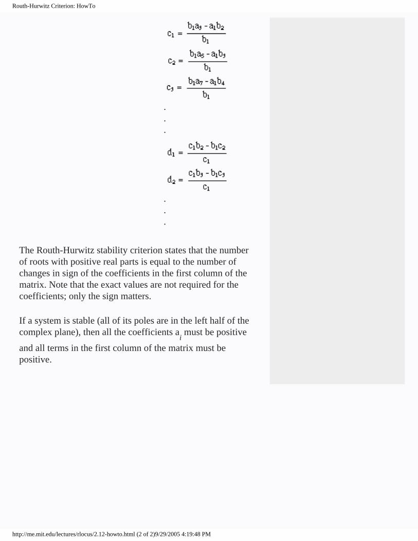
The Routh-Hurwitz stability criterion states that the number of roots with positive real parts is equal to the number of changes in sign of the coefficients in the first column of the matrix. Note that the exact values are not required for the coefficients; only the sign matters.
If a system is stable (all of its poles are in the left half of the complex plane), then all the coefficients a
i must be positive
and all terms in the first column of the matrix must be positive.
http://me.mit.edu/lectures/rlocus/2.12-howto.html (2 of 2)9/29/2005 4:19:48 PM
Routh-Hurwitz Criterion: Examples
Routh-Hurwitz Criterion
Goals Rationale HowTo Examples
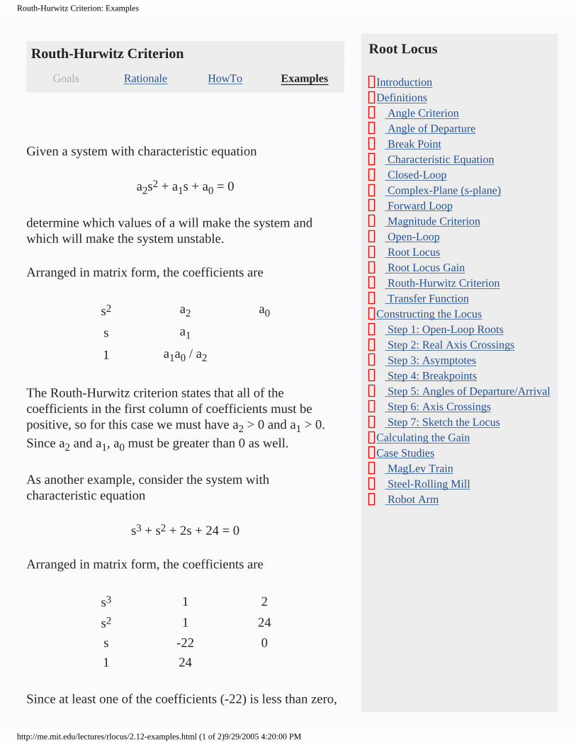
Given a system with characteristic equation
a2s2 + a1s + a0 = 0
determine which values of a will make the system and which will make the system unstable.
Arranged in matrix form, the coefficients are
s2 a2 a0
s a1
1 a1a0 / a2
The Routh-Hurwitz criterion states that all of the coefficients in the first column of coefficients must be positive, so for this case we must have a2 > 0 and a1 > 0.
Since a2 and a1, a0 must be greater than 0 as well.
As another example, consider the system with characteristic equation
s3 + s2 + 2s + 24 = 0
Arranged in matrix form, the coefficients are
s3 1 2
s2 1 24
s -22 0
1 24
Since at least one of the coefficients (-22) is less than zero,
Root Locus
IntroductionDefinitions Angle Criterion Angle of Departure Break Point Characteristic Equation Closed-Loop Complex-Plane (s-plane) Forward Loop Magnitude Criterion Open-Loop Root Locus Root Locus Gain Routh-Hurwitz Criterion Transfer FunctionConstructing the Locus Step 1: Open-Loop Roots Step 2: Real Axis Crossings Step 3: Asymptotes Step 4: Breakpoints Step 5: Angles of Departure/Arrival Step 6: Axis Crossings Step 7: Sketch the LocusCalculating the GainCase Studies MagLev Train Steel-Rolling Mill Robot Arm
http://me.mit.edu/lectures/rlocus/2.12-examples.html (1 of 2)9/29/2005 4:20:00 PM
Routh-Hurwitz Criterion: Examples
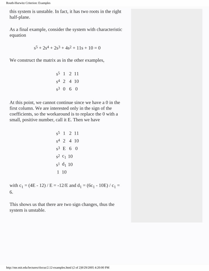
this system is unstable. In fact, it has two roots in the right half-plane.
As a final example, consider the system with characteristic equation
s5 + 2s4 + 2s3 + 4s2 + 11s + 10 = 0
We construct the matrix as in the other examples,
s5 1 2 11
s4 2 4 10
s3 0 6 0
At this point, we cannot continue since we have a 0 in the first column. We are interested only in the sign of the coefficients, so the workaround is to replace the 0 with a small, positive number, call it E. Then we have
s5 1 2 11
s4 2 4 10
s3 E 6 0
s2 c1 10
s1 d1 10
1 10
with c1 = (4E - 12) / E = -12/E and d1 = (6c1 - 10E) / c1 =
6.
This shows us that there are two sign changes, thus the system is unstable.
http://me.mit.edu/lectures/rlocus/2.12-examples.html (2 of 2)9/29/2005 4:20:00 PM
Transfer Function: Examples
Transfer Function
Goals Rationale HowTo Examples
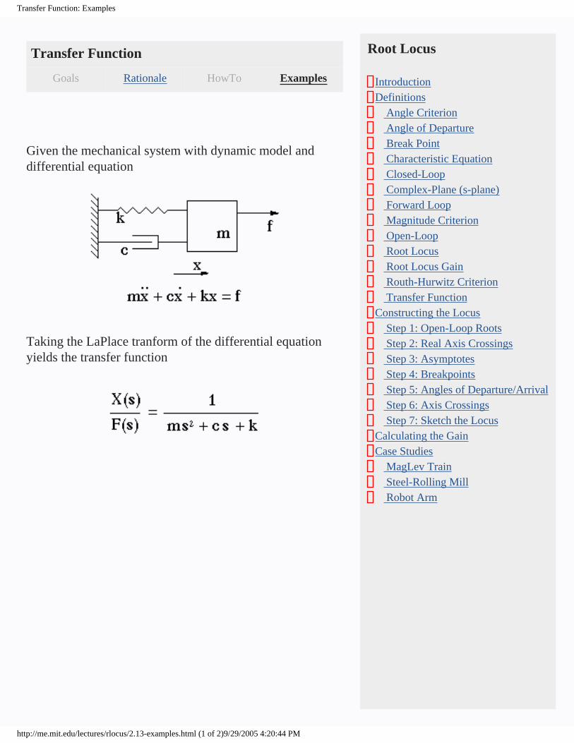
Given the mechanical system with dynamic model and differential equation
Taking the LaPlace tranform of the differential equation yields the transfer function
Root Locus
IntroductionDefinitions Angle Criterion Angle of Departure Break Point Characteristic Equation Closed-Loop Complex-Plane (s-plane) Forward Loop Magnitude Criterion Open-Loop Root Locus Root Locus Gain Routh-Hurwitz Criterion Transfer FunctionConstructing the Locus Step 1: Open-Loop Roots Step 2: Real Axis Crossings Step 3: Asymptotes Step 4: Breakpoints Step 5: Angles of Departure/Arrival Step 6: Axis Crossings Step 7: Sketch the LocusCalculating the GainCase Studies MagLev Train Steel-Rolling Mill Robot Arm
http://me.mit.edu/lectures/rlocus/2.13-examples.html (1 of 2)9/29/2005 4:20:44 PM

Transfer Function: Examples
http://me.mit.edu/lectures/rlocus/2.13-examples.html (2 of 2)9/29/2005 4:20:44 PM
Constructing the Locus: Rationale
Constructing the Locus
Goals Rationale HowTo Examples
In many cases, the designer of a control system needs a quick-and-dirty estimate of the behavior of the resulting closed-loop system. A root locus provides exactly this kind of information.
Root Locus
IntroductionDefinitions Angle Criterion Angle of Departure Break Point Characteristic Equation Closed-Loop Complex-Plane (s-plane) Forward Loop Magnitude Criterion Open-Loop Root Locus Root Locus Gain Routh-Hurwitz Criterion Transfer FunctionConstructing the Locus Step 1: Open-Loop Roots Step 2: Real Axis Crossings Step 3: Asymptotes Step 4: Breakpoints Step 5: Angles of Departure/Arrival Step 6: Axis Crossings Step 7: Sketch the LocusCalculating the GainCase Studies MagLev Train Steel-Rolling Mill Robot Arm
http://me.mit.edu/lectures/rlocus/3-rationale.html (1 of 2)9/29/2005 4:21:01 PM

Constructing the Locus: Rationale
http://me.mit.edu/lectures/rlocus/3-rationale.html (2 of 2)9/29/2005 4:21:01 PM
Constructing the Locus: HowTo
Constructing the Locus
Goals Rationale HowTo Examples
There are 7 steps to drawing a root locus.
1. Draw the forward-loop poles and zeros. 2. Draw the part of the locus that lies on the real axis. 3. Locate the centroid and sketch the asymptotes. 4. Determine the break point locations. 5. Determine the angles of arrival/departure. 6. Calculate the imaginary axis crossings. 7. Draw the rest of the locus.
Notice that you only have to draw the locus in the upper or lower half-plane. The root locus is always symmetric about the real axis.
Each of these steps is covered in more detail in the listing at right. Select the 'Examples' option to see all of the steps applied to a single system.
Root Locus
IntroductionDefinitions Angle Criterion Angle of Departure Break Point Characteristic Equation Closed-Loop Complex-Plane (s-plane) Forward Loop Magnitude Criterion Open-Loop Root Locus Root Locus Gain Routh-Hurwitz Criterion Transfer FunctionConstructing the Locus Step 1: Open-Loop Roots Step 2: Real Axis Crossings Step 3: Asymptotes Step 4: Breakpoints Step 5: Angles of Departure/Arrival Step 6: Axis Crossings Step 7: Sketch the LocusCalculating the GainCase Studies MagLev Train Steel-Rolling Mill Robot Arm
http://me.mit.edu/lectures/rlocus/3-howto.html (1 of 2)9/29/2005 4:23:40 PM

Constructing the Locus: HowTo
http://me.mit.edu/lectures/rlocus/3-howto.html (2 of 2)9/29/2005 4:23:40 PM
Constructing the Locus: Examples
Constructing the Locus
Goals Rationale HowTo Examples
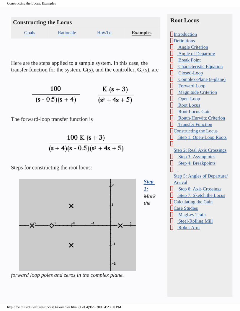
Here are the steps applied to a sample system. In this case, the transfer function for the system, G(s), and the controller, Gc(s), are
The forward-loop transfer function is
Steps for constructing the root locus:
Step 1: Mark the
forward loop poles and zeros in the complex plane.
Root Locus
IntroductionDefinitions Angle Criterion Angle of Departure Break Point Characteristic Equation Closed-Loop Complex-Plane (s-plane) Forward Loop Magnitude Criterion Open-Loop Root Locus Root Locus Gain Routh-Hurwitz Criterion Transfer FunctionConstructing the Locus Step 1: Open-Loop Roots Step 2: Real Axis Crossings Step 3: Asymptotes Step 4: Breakpoints Step 5: Angles of Departure/Arrival Step 6: Axis Crossings Step 7: Sketch the LocusCalculating the GainCase Studies MagLev Train Steel-Rolling Mill Robot Arm
http://me.mit.edu/lectures/rlocus/3-examples.html (1 of 4)9/29/2005 4:23:50 PM

Constructing the Locus: Examples
Step 2: Draw the real-axis part of the locus.
Step 3: Locate the
centroid and draw the asymptotes (if any).
http://me.mit.edu/lectures/rlocus/3-examples.html (2 of 4)9/29/2005 4:23:50 PM
Constructing the Locus: Examples
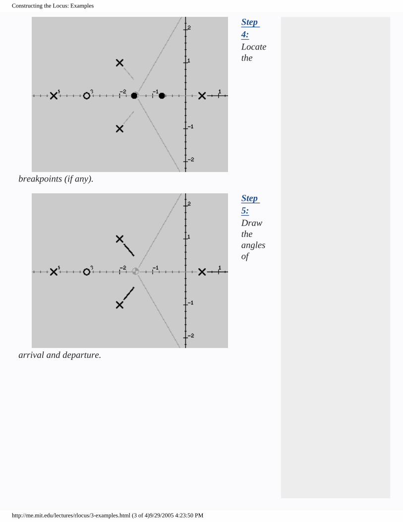
Step 4: Locate the
breakpoints (if any).
Step 5: Draw the angles of
arrival and departure.
http://me.mit.edu/lectures/rlocus/3-examples.html (3 of 4)9/29/2005 4:23:50 PM
Constructing the Locus: Examples
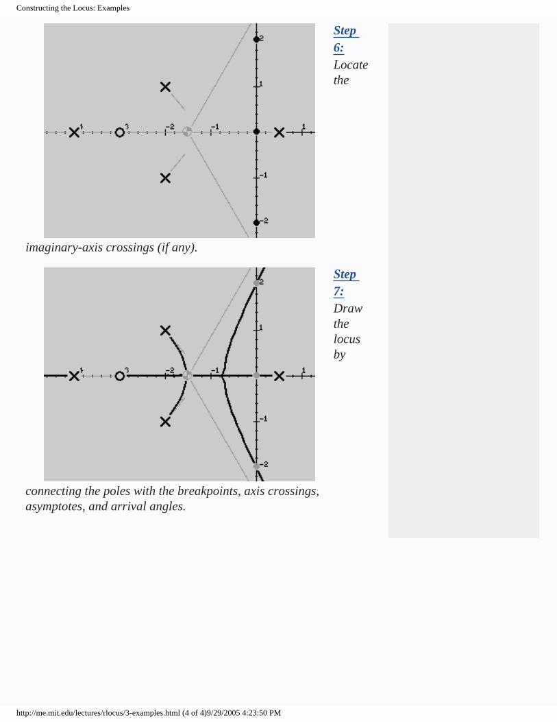
Step 6: Locate the
imaginary-axis crossings (if any).
Step 7: Draw the locus by
connecting the poles with the breakpoints, axis crossings, asymptotes, and arrival angles.
http://me.mit.edu/lectures/rlocus/3-examples.html (4 of 4)9/29/2005 4:23:50 PM

Step 1: Open-Loop Roots: HowTo
Step 1: Open-Loop Roots
Goals Rationale HowTo Examples
Draw the poles and zeros exactly as they appear in the forward-loop system. Include all of the poles and zeros, i.e. poles and zeros of both the controller and the uncontrolled system.
By convention, poles are represented with an X, zeros are represented with an O.
The poles will be the starting points of the loci, and the zeros will be the ending points.
Root Locus
IntroductionDefinitions Angle Criterion Angle of Departure Break Point Characteristic Equation Closed-Loop Complex-Plane (s-plane) Forward Loop Magnitude Criterion Open-Loop Root Locus Root Locus Gain Routh-Hurwitz Criterion Transfer FunctionConstructing the Locus Step 1: Open-Loop Roots Step 2: Real Axis Crossings Step 3: Asymptotes Step 4: Breakpoints Step 5: Angles of Departure/Arrival Step 6: Axis Crossings Step 7: Sketch the LocusCalculating the GainCase Studies MagLev Train Steel-Rolling Mill Robot Arm
http://me.mit.edu/lectures/rlocus/3.1-howto.html (1 of 2)9/29/2005 4:26:34 PM

Step 1: Open-Loop Roots: HowTo
http://me.mit.edu/lectures/rlocus/3.1-howto.html (2 of 2)9/29/2005 4:26:34 PM
Step 1: Open-Loop Roots: Examples
Step 1: Open-Loop Roots
Goals Rationale HowTo Examples
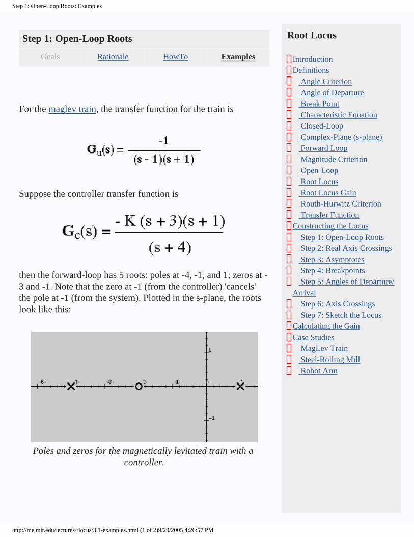
For the maglev train, the transfer function for the train is
Suppose the controller transfer function is
then the forward-loop has 5 roots: poles at -4, -1, and 1; zeros at -3 and -1. Note that the zero at -1 (from the controller) 'cancels' the pole at -1 (from the system). Plotted in the s-plane, the roots look like this:
Poles and zeros for the magnetically levitated train with a controller.
Root Locus
IntroductionDefinitions Angle Criterion Angle of Departure Break Point Characteristic Equation Closed-Loop Complex-Plane (s-plane) Forward Loop Magnitude Criterion Open-Loop Root Locus Root Locus Gain Routh-Hurwitz Criterion Transfer FunctionConstructing the Locus Step 1: Open-Loop Roots Step 2: Real Axis Crossings Step 3: Asymptotes Step 4: Breakpoints Step 5: Angles of Departure/Arrival Step 6: Axis Crossings Step 7: Sketch the LocusCalculating the GainCase Studies MagLev Train Steel-Rolling Mill Robot Arm
http://me.mit.edu/lectures/rlocus/3.1-examples.html (1 of 2)9/29/2005 4:26:57 PM

Step 1: Open-Loop Roots: Examples
http://me.mit.edu/lectures/rlocus/3.1-examples.html (2 of 2)9/29/2005 4:26:57 PM
Step 2: Real Axis Crossings: HowTo
Step 2: Real Axis Crossings
Goals Rationale HowTo Examples
Start at positive infinity on the real axis. Move toward the origin until you encounter a pole or zero on the real axis. Draw a line from this pole/zero until the next pole or zero on the real axis. If there are no more poles/zeros, the locus extends to negative infinity on the real axis. Otherwise, the locus starts again at the next pole/zero and continues to its successor, and so on.
If there are no poles or zeros on the real axis, then there will be no real axis component to the root locus.
Some systems have more than one pole or zero at the same location (this indicates a double, triple, or even higher order root to the characteristic equation). If there are an odd number of poles or zeros at the same location, the real axis part of the locus continues after the location of that pole/zero. If the number of poles/zeros at the location is even, the real axis part of the locus stops at that location.
Root Locus
IntroductionDefinitions Angle Criterion Angle of Departure Break Point Characteristic Equation Closed-Loop Complex-Plane (s-plane) Forward Loop Magnitude Criterion Open-Loop Root Locus Root Locus Gain Routh-Hurwitz Criterion Transfer FunctionConstructing the Locus Step 1: Open-Loop Roots Step 2: Real Axis Crossings Step 3: Asymptotes Step 4: Breakpoints Step 5: Angles of Departure/Arrival Step 6: Axis Crossings Step 7: Sketch the LocusCalculating the GainCase Studies MagLev Train Steel-Rolling Mill Robot Arm
http://me.mit.edu/lectures/rlocus/3.2-howto.html (1 of 2)9/29/2005 4:28:53 PM

Step 2: Real Axis Crossings: HowTo
http://me.mit.edu/lectures/rlocus/3.2-howto.html (2 of 2)9/29/2005 4:28:53 PM

Step 2: Real Axis Crossings: Examples
Step 2: Real Axis Crossings
Goals Rationale HowTo Examples
In the magnetically levitated train example, the real axis part of the locus is the entire locus. To see the system responses in the time domain that correspond to this root locus, go to the case study.
Root Locus
IntroductionDefinitions Angle Criterion Angle of Departure Break Point Characteristic Equation Closed-Loop Complex-Plane (s-plane) Forward Loop Magnitude Criterion Open-Loop Root Locus Root Locus Gain Routh-Hurwitz Criterion Transfer FunctionConstructing the Locus Step 1: Open-Loop Roots Step 2: Real Axis Crossings Step 3: Asymptotes Step 4: Breakpoints Step 5: Angles of Departure/Arrival Step 6: Axis Crossings Step 7: Sketch the LocusCalculating the GainCase Studies MagLev Train Steel-Rolling Mill Robot Arm
http://me.mit.edu/lectures/rlocus/3.2-examples.html (1 of 2)9/29/2005 4:29:40 PM

Step 2: Real Axis Crossings: Examples
Pick any point on the real axis. If there are an odd number of roots to the right of that point, that point on the axis is a part of the locus.
If there is a multiple root, then the real axis part depends on whether there are an even or odd number of roots at the same point.
http://me.mit.edu/lectures/rlocus/3.2-examples.html (2 of 2)9/29/2005 4:29:40 PM

Step 3: Asymptotes: HowTo
Step 3: Asymptotes
Goals Rationale HowTo Examples
First determine how many poles, n, and how many zeros, m, are in the system, then locate the centroid. The number of asymptotes is equal to the difference between the number of poles and the number of zeros. The location of the centroid on the real axis is given by:
where pi and zj are the poles and zeros, respectively. Since pi and
zj are symmetric about the real axis, their imaginary parts get
cancelled out.
Once you have located the centroid, draw the asymptotes at the proper angles. The asymptotes will leave the centroid at angles defined by
Note that because of the symmetry, the asymptotes must assume one of the following configurations, for n-m = 1,2,3,4,5.
Root Locus
IntroductionDefinitions Angle Criterion Angle of Departure Break Point Characteristic Equation Closed-Loop Complex-Plane (s-plane) Forward Loop Magnitude Criterion Open-Loop Root Locus Root Locus Gain Routh-Hurwitz Criterion Transfer FunctionConstructing the Locus Step 1: Open-Loop Roots Step 2: Real Axis Crossings Step 3: Asymptotes Step 4: Breakpoints Step 5: Angles of Departure/Arrival Step 6: Axis Crossings Step 7: Sketch the LocusCalculating the GainCase Studies MagLev Train Steel-Rolling Mill Robot Arm
http://me.mit.edu/lectures/rlocus/3.3-howto.html (1 of 2)9/29/2005 4:30:26 PM

Step 3: Asymptotes: HowTo
http://me.mit.edu/lectures/rlocus/3.3-howto.html (2 of 2)9/29/2005 4:30:26 PM
Step 3: Asymptotes: Examples
Step 3: Asymptotes
Goals Rationale HowTo Examples
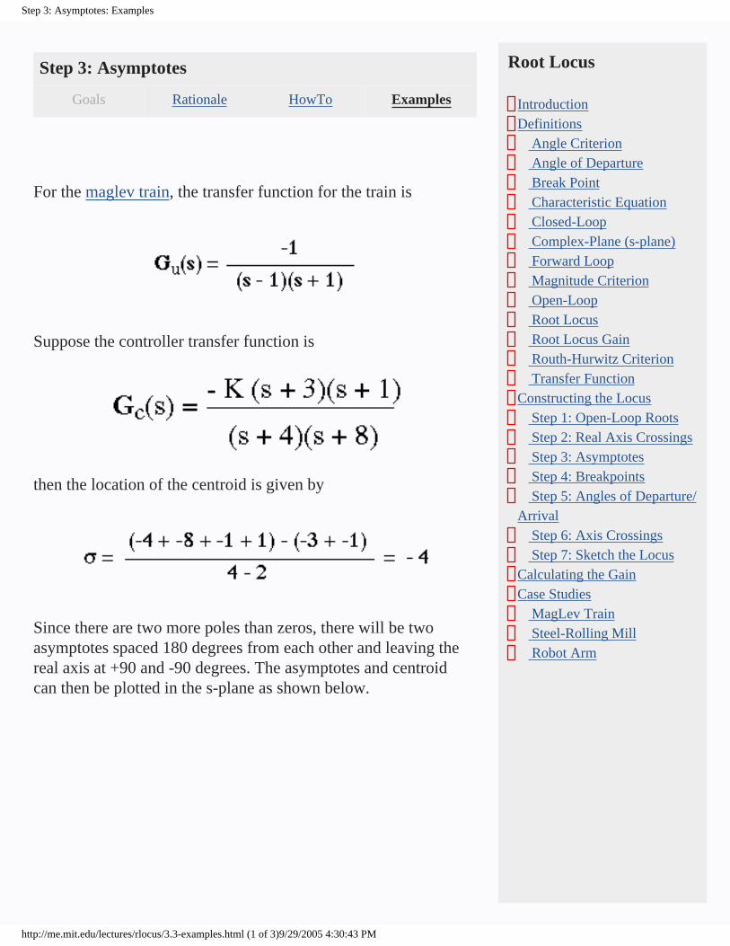
For the maglev train, the transfer function for the train is
Suppose the controller transfer function is
then the location of the centroid is given by
Since there are two more poles than zeros, there will be two asymptotes spaced 180 degrees from each other and leaving the real axis at +90 and -90 degrees. The asymptotes and centroid can then be plotted in the s-plane as shown below.
Root Locus
IntroductionDefinitions Angle Criterion Angle of Departure Break Point Characteristic Equation Closed-Loop Complex-Plane (s-plane) Forward Loop Magnitude Criterion Open-Loop Root Locus Root Locus Gain Routh-Hurwitz Criterion Transfer FunctionConstructing the Locus Step 1: Open-Loop Roots Step 2: Real Axis Crossings Step 3: Asymptotes Step 4: Breakpoints Step 5: Angles of Departure/Arrival Step 6: Axis Crossings Step 7: Sketch the LocusCalculating the GainCase Studies MagLev Train Steel-Rolling Mill Robot Arm
http://me.mit.edu/lectures/rlocus/3.3-examples.html (1 of 3)9/29/2005 4:30:43 PM
Step 3: Asymptotes: Examples
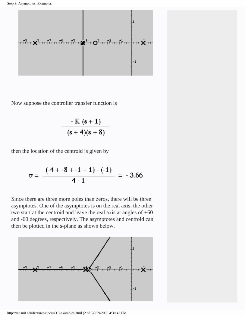
Now suppose the controller transfer function is
then the location of the centroid is given by
Since there are three more poles than zeros, there will be three asymptotes. One of the asymptotes is on the real axis, the other two start at the centroid and leave the real axis at angles of +60 and -60 degrees, respectively. The asymptotes and centroid can then be plotted in the s-plane as shown below.
http://me.mit.edu/lectures/rlocus/3.3-examples.html (2 of 3)9/29/2005 4:30:43 PM

Step 3: Asymptotes: Examples
http://me.mit.edu/lectures/rlocus/3.3-examples.html (3 of 3)9/29/2005 4:30:43 PM

Step 5: Angles of Departure/Arrival: HowTo
Step 5: Angles of Departure/Arrival
Goals Rationale HowTo Examples
angle of departure. At each complex pole, add up the angles from the zeros to the current pole, then subtract the angles from the other poles to the current pole. In mathematical terms, for a given pole, the angle of departure is
where is the angle between the ith pole and the given pole,
and is the angle between the jth zero and the given pole.
and can be calculated using trigonometry.
angle of arrival. At each zero, add up the angles from the poles to the current zero, then subtract the angles from the other zeros to the current zero. In mathematical terms, for a given zero, the angle of departure is
where is the angle between the ith pole the the given zero, and
is the angle between the jth zero and the given zero.
By convention, the arrival and departure angles are measured relative to the real axis, so that the positive real axis is 0. Graphically, the angles look like this
Root Locus
IntroductionDefinitions Angle Criterion Angle of Departure Break Point Characteristic Equation Closed-Loop Complex-Plane (s-plane) Forward Loop Magnitude Criterion Open-Loop Root Locus Root Locus Gain Routh-Hurwitz Criterion Transfer FunctionConstructing the Locus Step 1: Open-Loop Roots Step 2: Real Axis Crossings Step 3: Asymptotes Step 4: Breakpoints Step 5: Angles of Departure/Arrival Step 6: Axis Crossings Step 7: Sketch the LocusCalculating the GainCase Studies MagLev Train Steel-Rolling Mill Robot Arm
http://me.mit.edu/lectures/rlocus/3.5-howto.html (1 of 2)9/29/2005 4:40:16 PM

Step 5: Angles of Departure/Arrival: HowTo
Note that single poles and zeros on the real axis will always have arrival/departure angles equal to 0 or 180 degrees due to the symmetry of the complex conjugates.
http://me.mit.edu/lectures/rlocus/3.5-howto.html (2 of 2)9/29/2005 4:40:16 PM
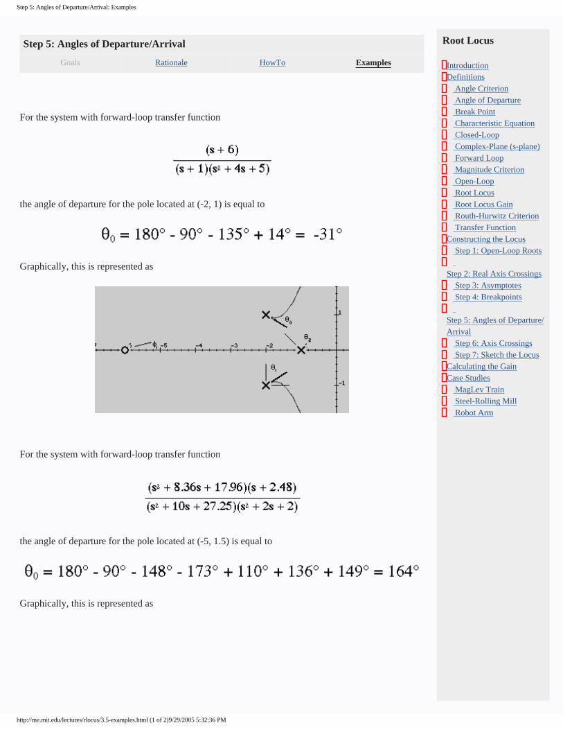
Step 5: Angles of Departure/Arrival: Examples
Step 5: Angles of Departure/Arrival
Goals Rationale HowTo Examples
For the system with forward-loop transfer function
the angle of departure for the pole located at (-2, 1) is equal to
Graphically, this is represented as
For the system with forward-loop transfer function
the angle of departure for the pole located at (-5, 1.5) is equal to
Graphically, this is represented as
Root Locus
IntroductionDefinitions Angle Criterion Angle of Departure Break Point Characteristic Equation Closed-Loop Complex-Plane (s-plane) Forward Loop Magnitude Criterion Open-Loop Root Locus Root Locus Gain Routh-Hurwitz Criterion Transfer FunctionConstructing the Locus Step 1: Open-Loop Roots Step 2: Real Axis Crossings Step 3: Asymptotes Step 4: Breakpoints Step 5: Angles of Departure/Arrival Step 6: Axis Crossings Step 7: Sketch the LocusCalculating the GainCase Studies MagLev Train Steel-Rolling Mill Robot Arm
http://me.mit.edu/lectures/rlocus/3.5-examples.html (1 of 2)9/29/2005 5:32:36 PM
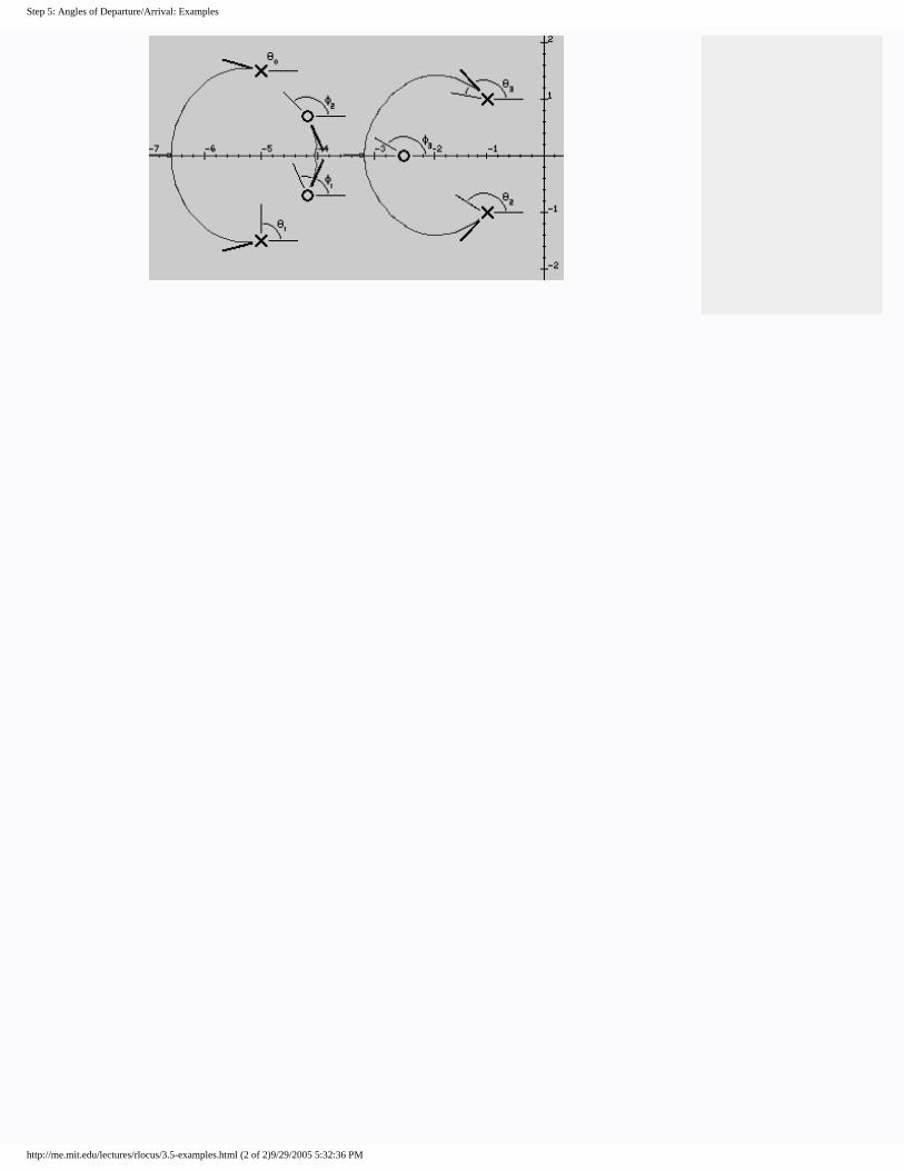
Step 5: Angles of Departure/Arrival: Examples
http://me.mit.edu/lectures/rlocus/3.5-examples.html (2 of 2)9/29/2005 5:32:36 PM

Step 6: Axis Crossings: HowTo
Step 6: Axis Crossings
Goals Rationale HowTo Examples
Not every locus will have imaginary axis crossings. First determine if the locus will definitely cross the imaginary axis (for example, if there are more than two asymptotes), or if there is a good chance that the locus crosses the imaginary axis (for example, if there are poles or zeros close to the imaginary axis and/or the arrival/departure angles lead you to believe that the locus may cross).
There are three ways to find the points where the locus intersects the imaginary axis:
● trial and error (bracketing) ● the Routh-Hurwitz stability criterion ● solving for omega and K
Which method to use depends on how accurately you need the locations of the axis crossings.
Trial and error. Start at the origin in the complex plane. Move up the imaginary axis in discrete steps and calculate the phase of the forward loop transfer function at each step. If the phase at the last point was less than 180 degrees and the phase at the current point is greater than 180 degrees (or vice versa) then an axis crossing lies between the two points. If the phase is equal to 180 degrees, then the point is on the locus and is an imaginary axis crossing point.
By bracketing regions on the imaginary axis, you can often quickly determine the axis crossings using this method. Rather than working up from the origin in regular steps, bracketing uses a binary search approach in which two points are tested, then another point is chosen based on whether or not there was a phase change between the two points. If there was a phase change, the third point is chosen between the two, of not, it is chosen outside the
Root Locus
IntroductionDefinitions Angle Criterion Angle of Departure Break Point Characteristic Equation Closed-Loop Complex-Plane (s-plane) Forward Loop Magnitude Criterion Open-Loop Root Locus Root Locus Gain Routh-Hurwitz Criterion Transfer FunctionConstructing the Locus Step 1: Open-Loop Roots Step 2: Real Axis Crossings Step 3: Asymptotes Step 4: Breakpoints Step 5: Angles of Departure/Arrival Step 6: Axis Crossings Step 7: Sketch the LocusCalculating the GainCase Studies MagLev Train Steel-Rolling Mill Robot Arm
http://me.mit.edu/lectures/rlocus/3.6-howto.html (1 of 2)9/29/2005 5:33:32 PM

Step 6: Axis Crossings: HowTo
two.
Using the Routh-Hurwitz stability criterion. From the characteristic equation, create the matrix of coefficients as you would to determine the stability of the system. Then from the matrix of coefficients, solve for K such that the stability criterion is met. Then solve for s to determine where on the imaginary axis the gain K is in effect. Note that this method can be very difficult to use, especially for systems with many poles and zeros.
Solving for omega and K. Let s = j omega in the characteristic equation, equating both the real and imaginary parts to zero, then solve for omega and K. The values of omega are the frequencies at which the root loci cross the imaginary axis. The value of K is the root locus gain at which the crossing occurs.
http://me.mit.edu/lectures/rlocus/3.6-howto.html (2 of 2)9/29/2005 5:33:32 PM
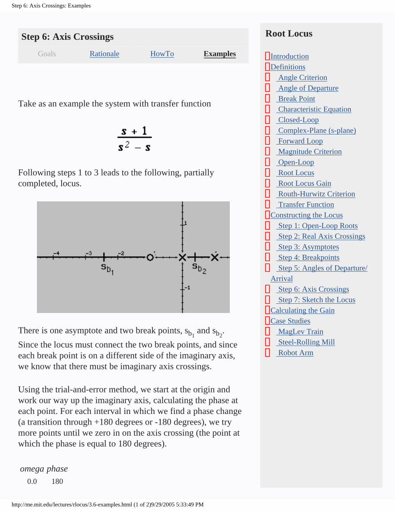
Step 6: Axis Crossings: Examples
Step 6: Axis Crossings
Goals Rationale HowTo Examples
Take as an example the system with transfer function
Following steps 1 to 3 leads to the following, partially completed, locus.
There is one asymptote and two break points, sb1 and sb2
.
Since the locus must connect the two break points, and since each break point is on a different side of the imaginary axis, we know that there must be imaginary axis crossings.
Using the trial-and-error method, we start at the origin and work our way up the imaginary axis, calculating the phase at each point. For each interval in which we find a phase change (a transition through +180 degrees or -180 degrees), we try more points until we zero in on the axis crossing (the point at which the phase is equal to 180 degrees).
omega phase0.0 180
Root Locus
IntroductionDefinitions Angle Criterion Angle of Departure Break Point Characteristic Equation Closed-Loop Complex-Plane (s-plane) Forward Loop Magnitude Criterion Open-Loop Root Locus Root Locus Gain Routh-Hurwitz Criterion Transfer FunctionConstructing the Locus Step 1: Open-Loop Roots Step 2: Real Axis Crossings Step 3: Asymptotes Step 4: Breakpoints Step 5: Angles of Departure/Arrival Step 6: Axis Crossings Step 7: Sketch the LocusCalculating the GainCase Studies MagLev Train Steel-Rolling Mill Robot Arm
http://me.mit.edu/lectures/rlocus/3.6-examples.html (1 of 2)9/29/2005 5:33:49 PM

Step 6: Axis Crossings: Examples
0.25 242
0.5 217
0.75 196
1.0 180
1.5 158
2.0 144
2.5 134
3.0 126
In this case, the transition occurs at (0,1) and (0,-1). The root locus for this system is therefore
http://me.mit.edu/lectures/rlocus/3.6-examples.html (2 of 2)9/29/2005 5:33:49 PM

Step 7: Sketch the Locus: Examples
Step 7: Sketch the Locus
Goals Rationale HowTo Examples
These are some root locus plots for a variety of systems. They include the construction marks for arrival/departure angles, asymptotes, break points, and axis crossings. Note that in some cases, a slight change in pole or zero coordinates can result in a markedly different locus. Note also, however, that such small changes to the roots will not change more general locus characteristics, such as the number of asymptotes.
Locus for a system with three poles and no zeros.
Root Locus
IntroductionDefinitions Angle Criterion Angle of Departure Break Point Characteristic Equation Closed-Loop Complex-Plane (s-plane) Forward Loop Magnitude Criterion Open-Loop Root Locus Root Locus Gain Routh-Hurwitz Criterion Transfer FunctionConstructing the Locus Step 1: Open-Loop Roots Step 2: Real Axis Crossings Step 3: Asymptotes Step 4: Breakpoints Step 5: Angles of Departure/Arrival Step 6: Axis Crossings Step 7: Sketch the LocusCalculating the GainCase Studies MagLev Train Steel-Rolling Mill Robot Arm
http://me.mit.edu/lectures/rlocus/3.7-examples.html (1 of 4)9/29/2005 5:37:11 PM
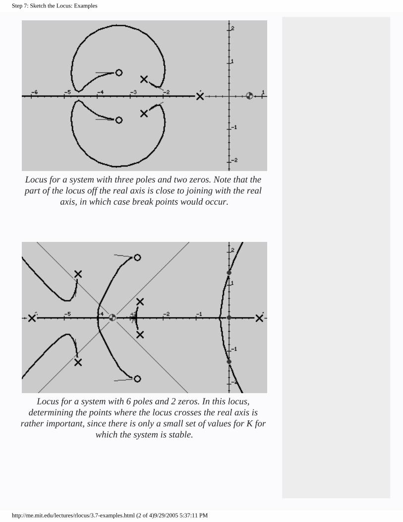
Step 7: Sketch the Locus: Examples
Locus for a system with three poles and two zeros. Note that the part of the locus off the real axis is close to joining with the real
axis, in which case break points would occur.
Locus for a system with 6 poles and 2 zeros. In this locus, determining the points where the locus crosses the real axis is
rather important, since there is only a small set of values for K for which the system is stable.
http://me.mit.edu/lectures/rlocus/3.7-examples.html (2 of 4)9/29/2005 5:37:11 PM
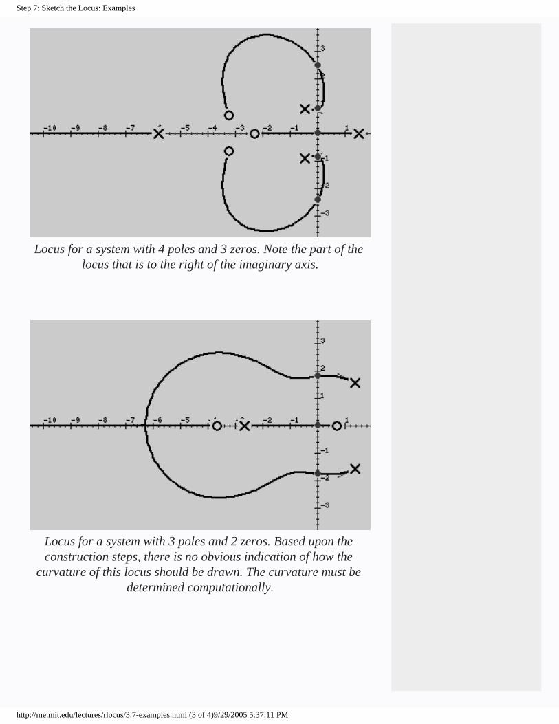
Step 7: Sketch the Locus: Examples
Locus for a system with 4 poles and 3 zeros. Note the part of the locus that is to the right of the imaginary axis.
Locus for a system with 3 poles and 2 zeros. Based upon the construction steps, there is no obvious indication of how the
curvature of this locus should be drawn. The curvature must be determined computationally.
http://me.mit.edu/lectures/rlocus/3.7-examples.html (3 of 4)9/29/2005 5:37:11 PM

Step 7: Sketch the Locus: Examples
Locus for a system with 5 poles and 2 zeros. Compare this locus with that in the next image.
Locus for a system with 5 poles and 2 zeros. Compare this locus with that in the previous image. A slight change in the position of the zeros changes the shape of the locus, but does not change the
system behavior for large values of the root locus gain.
http://me.mit.edu/lectures/rlocus/3.7-examples.html (4 of 4)9/29/2005 5:37:11 PM
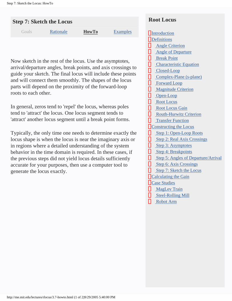
Step 7: Sketch the Locus: HowTo
Step 7: Sketch the Locus
Goals Rationale HowTo Examples
Now sketch in the rest of the locus. Use the asymptotes, arrival/departure angles, break points, and axis crossings to guide your sketch. The final locus will include these points and will connect them smoothly. The shapes of the locus parts will depend on the proximity of the forward-loop roots to each other.
In general, zeros tend to 'repel' the locus, whereas poles tend to 'attract' the locus. One locus segment tends to 'attract' another locus segment until a break point forms.
Typically, the only time one needs to determine exactly the locus shape is when the locus is near the imaginary axis or in regions where a detailed understanding of the system behavior in the time domain is required. In these cases, if the previous steps did not yield locus details sufficiently accurate for your purposes, then use a computer tool to generate the locus exactly.
Root Locus
IntroductionDefinitions Angle Criterion Angle of Departure Break Point Characteristic Equation Closed-Loop Complex-Plane (s-plane) Forward Loop Magnitude Criterion Open-Loop Root Locus Root Locus Gain Routh-Hurwitz Criterion Transfer FunctionConstructing the Locus Step 1: Open-Loop Roots Step 2: Real Axis Crossings Step 3: Asymptotes Step 4: Breakpoints Step 5: Angles of Departure/Arrival Step 6: Axis Crossings Step 7: Sketch the LocusCalculating the GainCase Studies MagLev Train Steel-Rolling Mill Robot Arm
http://me.mit.edu/lectures/rlocus/3.7-howto.html (1 of 2)9/29/2005 5:40:00 PM

Step 7: Sketch the Locus: HowTo
http://me.mit.edu/lectures/rlocus/3.7-howto.html (2 of 2)9/29/2005 5:40:00 PM

Steel-Rolling Mill: Examples
Steel-Rolling Mill
Goals Rationale HowTo Examples
The root locus for the steelrolling system with each controller is shown below.
root locus for controller 1
root locus for controller 2
Root Locus
IntroductionDefinitions Angle Criterion Angle of Departure Break Point Characteristic Equation Closed-Loop Complex-Plane (s-plane) Forward Loop Magnitude Criterion Open-Loop Root Locus Root Locus Gain Routh-Hurwitz Criterion Transfer FunctionConstructing the Locus Step 1: Open-Loop Roots Step 2: Real Axis Crossings Step 3: Asymptotes Step 4: Breakpoints Step 5: Angles of Departure/Arrival Step 6: Axis Crossings Step 7: Sketch the LocusCalculating the GainCase Studies MagLev Train Steel-Rolling Mill Robot Arm
http://me.mit.edu/lectures/rlocus/5.2-examples.html (1 of 2)9/29/2005 5:42:35 PM
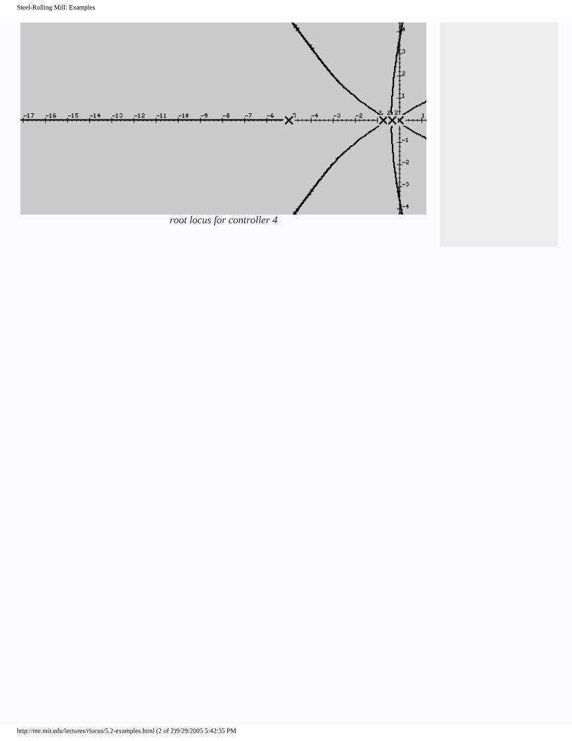
Steel-Rolling Mill: Examples
root locus for controller 4
http://me.mit.edu/lectures/rlocus/5.2-examples.html (2 of 2)9/29/2005 5:42:35 PM
Case Studies: Rationale
Case Studies
Goals Rationale HowTo Examples
This section contains case studies that illustrate the use of the root locus in some real control problems.
Once you have a transfer function to represent your system, applying the control principles is fairly straightforward. However, often you will find that, as you analyze the controller that you have designed, your model of the plant may need some adjustments or your controller's parameters must be tuned to make it more robust to disturbances that you did not anticipate. These characteristics are usually not obvious when you first start to work on a system, and typically require some experience to anticipate them when working with both the real system and the mathematical abstraction.
The cases in this section come from very different domains. From a control perspective, the domain does not matter much. Once the system has been modelled (i.e. once you have a transfer function for it), classic control theory applies whether the system is a rocket on its way out of the atmosphere, a monstrous chemical processing plant in northern Kentucky, or a bench-top robot arm driven by a DC motor.
The focus of this lecture is feedback control, not modelling. As you go through the cases you may find that a system could be modelled more accurately or that a slight design modification to the system would make designing the controller much easier.
Root Locus
IntroductionDefinitions Angle Criterion Angle of Departure Break Point Characteristic Equation Closed-Loop Complex-Plane (s-plane) Forward Loop Magnitude Criterion Open-Loop Root Locus Root Locus Gain Routh-Hurwitz Criterion Transfer FunctionConstructing the Locus Step 1: Open-Loop Roots Step 2: Real Axis Crossings Step 3: Asymptotes Step 4: Breakpoints Step 5: Angles of Departure/Arrival Step 6: Axis Crossings Step 7: Sketch the LocusCalculating the GainCase Studies MagLev Train Steel-Rolling Mill Robot Arm
http://me.mit.edu/lectures/rlocus/5-rationale.html (1 of 2)9/29/2005 5:46:02 PM

Case Studies: Rationale
http://me.mit.edu/lectures/rlocus/5-rationale.html (2 of 2)9/29/2005 5:46:02 PM
Step 4: Breakpoints: HowTo
Step 4: Breakpoints
Goals Rationale HowTo Examples
Perhaps the easiest way to find break points is by trial and error. First, determine the characteristic equation of the system in terms of K. In the vicinity of the suspected break point, substitute values for s in this equation. A break point occurs when when the characteristic equation is minimized.
To calculate the break point explicitly requires that you derive the derivative of the characteristic equation in terms of s then equate the derivative to 0 and solve that equation for K and s.
Root Locus
IntroductionDefinitions Angle Criterion Angle of Departure Break Point Characteristic Equation Closed-Loop Complex-Plane (s-plane) Forward Loop Magnitude Criterion Open-Loop Root Locus Root Locus Gain Routh-Hurwitz Criterion Transfer FunctionConstructing the Locus Step 1: Open-Loop Roots Step 2: Real Axis Crossings Step 3: Asymptotes Step 4: Breakpoints Step 5: Angles of Departure/Arrival Step 6: Axis Crossings Step 7: Sketch the LocusCalculating the GainCase Studies MagLev Train Steel-Rolling Mill Robot Arm
http://me.mit.edu/lectures/rlocus/3.4-howto.html (1 of 2)10/23/2005 11:09:39 AM

Step 4: Breakpoints: HowTo
http://me.mit.edu/lectures/rlocus/3.4-howto.html (2 of 2)10/23/2005 11:09:39 AM
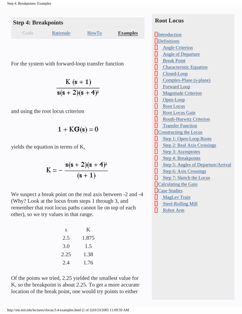
Step 4: Breakpoints: Examples
Step 4: Breakpoints
Goals Rationale HowTo Examples
For the system with forward-loop transfer function
and using the root locus criterion
yields the equation in terms of K,
We suspect a break point on the real axis between -2 and -4 (Why? Look at the locus from steps 1 through 3, and remember that root locus paths cannot lie on top of each other), so we try values in that range.
s K
2.5 1.875
3.0 1.5
2.25 1.38
2.4 1.76
Of the points we tried, 2.25 yielded the smallest value for K, so the breakpoint is about 2.25. To get a more accurate location of the break point, one would try points to either
Root Locus
IntroductionDefinitions Angle Criterion Angle of Departure Break Point Characteristic Equation Closed-Loop Complex-Plane (s-plane) Forward Loop Magnitude Criterion Open-Loop Root Locus Root Locus Gain Routh-Hurwitz Criterion Transfer FunctionConstructing the Locus Step 1: Open-Loop Roots Step 2: Real Axis Crossings Step 3: Asymptotes Step 4: Breakpoints Step 5: Angles of Departure/Arrival Step 6: Axis Crossings Step 7: Sketch the LocusCalculating the GainCase Studies MagLev Train Steel-Rolling Mill Robot Arm
http://me.mit.edu/lectures/rlocus/3.4-examples.html (1 of 2)10/23/2005 11:09:59 AM

Step 4: Breakpoints: Examples
side of 2.25 to locate the minimum.
http://me.mit.edu/lectures/rlocus/3.4-examples.html (2 of 2)10/23/2005 11:09:59 AM