Embed Size (px)
Citation preview

1
Computer Graphics
Course outline
Introduction Images and display techniques
Bases Gamma correction Aliasing and techniques to remedy Storage

2
Computer Graphics
Course outline
3D Perspective & 2D / 3D transformations Go from a 3D space to a 2D display device
Two paradigms for image synthesis Representation of curves and surfaces
Splines & co. Meshes
Realistic rendering by ray tracing Concepts and theoretical bases
3
Computer Graphics
Aliasing
« Aliasing » (crénelage in French) Appears during image synthesis or capture, during
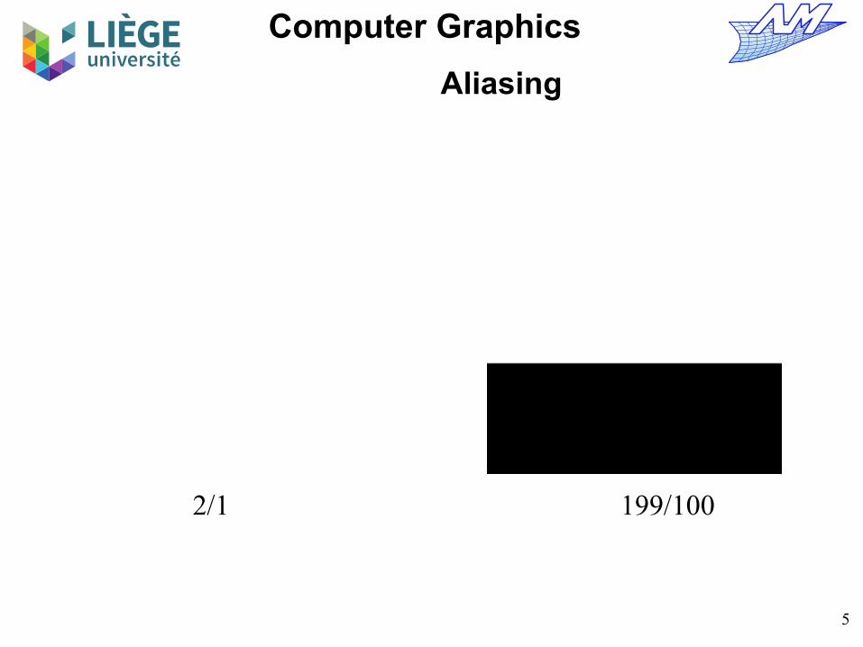
spatial discretization (transformation of a “continuous” image to discrete pixels) Small experiment : The test image is a series of black and white
lines, with an increasing density.
1 line/4 pixels 1/2

4
Computer Graphics
Aliasing
1/1 3/2
5
Computer Graphics
Aliasing
2/1 199/100

6
Computer Graphics
Aliasing
16/5
In fact, one should not have any spatial frequency that is higher than a given cutoff frequency, that depends on the sampling density.

7
Computer Graphics
Aliasing
Nyquist-Shannon theorem If the spectrum of a function doesn't contain frequencies higher than
e.g. B, then it is completely determined by a series of samples (in time, space …) separated by 1 / (2B) , or of frequency equal to 2B . 2B is the Nyquist frequency.
Otherwise, there is aliasing:
Signal reconstruction
Original signal
2fnyquist
2fnyquist
Fourrier transform (amplitude)
f̂ (ω)= ∫−∞
+∞
f (t)eiω t dt

8
Computer Graphics
Aliasing
Moiré patterns

9
Computer Graphics
Aliasing
How to limit aliasing ? By increasing the sampling density to respect Nyquist-
Shannon's theorem ? By filtering the signal with a low pass filter to be in the
window of Shannon's theorem for a given sampling density ?
A combination of both... ?

10
Computer Graphics
Aliasing
Increase the sampling density (or rate) Equivalent to increase the image resolution But : real life images are often fractal
High frequency details are such that spatial resolution is huge But : artificially generated images include sudden changes in
intensity (e.g. black lines on white background) Cf Fourier decomposition of a square signal :
Spectrum of a square signal : odd harmonics of amplitude 1/n ...
This solution alone is not working well.

11
Computer Graphics
Aliasing
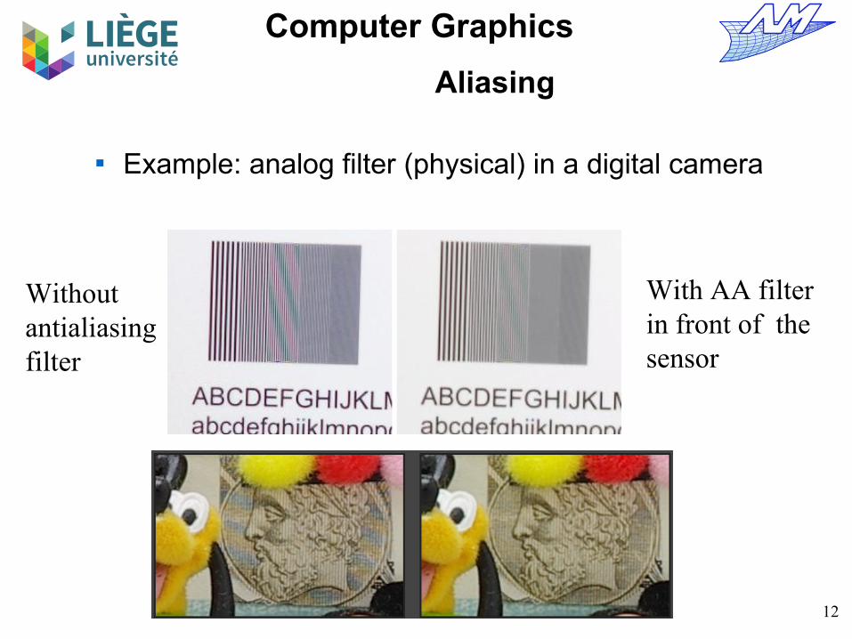
Analog lowpass filter For capturing devices, this must be done before the actual capture Makes slightly blurred image - but not too much! This is exactly what we find on the sensor of digital cameras : An AA
filter positioned between the lens, and the sensor. Many technologies are available.
12
Computer Graphics
Aliasing
Example: analog filter (physical) in a digital camera
Withoutantialiasingfilter
With AA filterin front of the sensor

13
Computer Graphics
Aliasing
Numerical low-pass filtering When one creates artificial images, no analog AA is possible The usual way is to use oversampling (sampling with a higher rate),
followed by a arithmetic mean to return to the actual (desired) sampling rate
It is also possible to introduce variability in the sampling positions (e.g. add a random contribution to the positions of sample in a pixel)
49x49 resolutionwith 4x4 oversampling
49x49 resolution W/O antialiasing
196x196 resolutionW/O antialiasing
Original image (continuous)

14
Computer Graphics
Aliasing
Simulation of an analog low-pass filter
Original image (continuous)
“Blurred”original image
49x49 resolution from the “blurred”
image
Reminder :49x49 resolution
with 4x4 oversampling
15
Computer Graphics
Aliasing
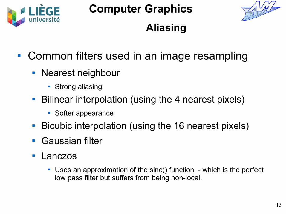
Common filters used in an image resampling Nearest neighbour
Strong aliasing
Bilinear interpolation (using the 4 nearest pixels) Softer appearance
Bicubic interpolation (using the 16 nearest pixels) Gaussian filter Lanczos
Uses an approximation of the sinc() function - which is the perfect low pass filter but suffers from being non-local.
16
Computer Graphics
Aliasing
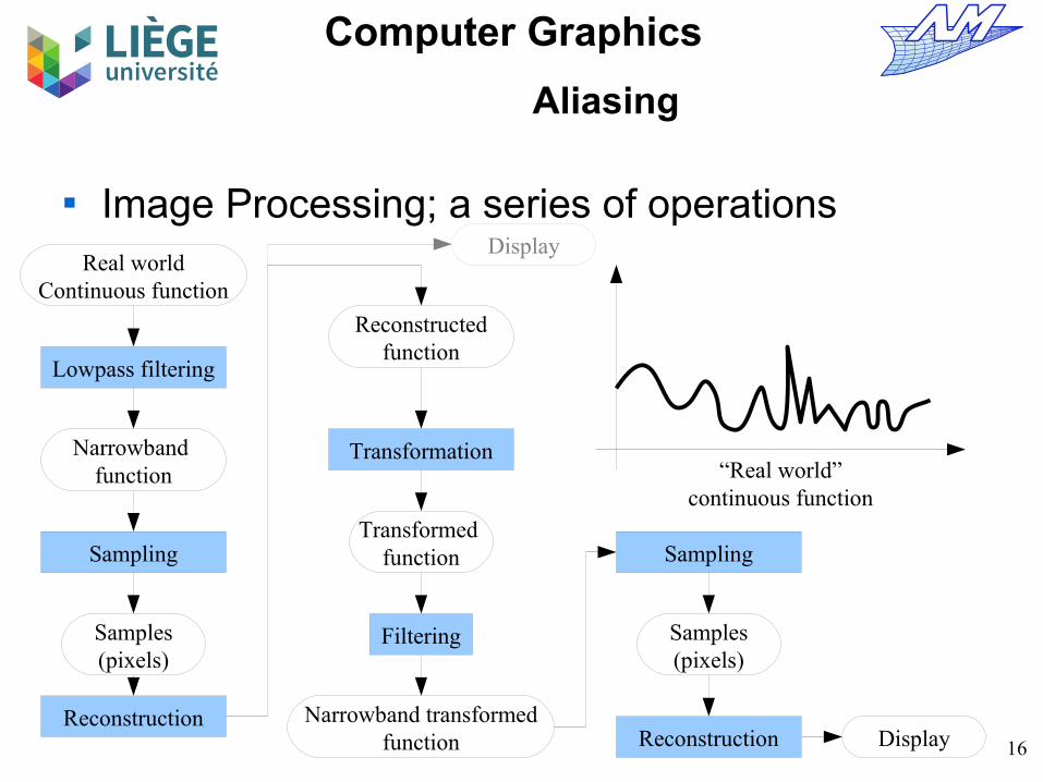
Image Processing; a series of operations
Sampling
Reconstruction
Transformation
Filtering
Sampling
Reconstruction
Lowpass filtering
Real worldContinuous function
Samples(pixels)
Narrowband function
Reconstructedfunction
Transformed function
Narrowband transformedfunction
Samples(pixels)
Display
Display
“Real world” continuous function

17
Computer Graphics
Aliasing
Image Processing; a series of operations
Sampling
Reconstruction
Transformation
Filtering
Sampling
Reconstruction
Lowpass filtering
Real worldContinuous function
Samples(pixels)
Narrowband function
Reconstructedfunction
Transformedfunction
Narrowband transformedfunction
Samples(pixels)
Display
Narrowband function

18
Computer Graphics
Aliasing
Image Processing; a series of operations
Sampling
Reconstruction
Transformation
Filtering
Sampling
Reconstruction
Lowpass filtering
Real worldContinuous function
Samples(pixels)
Narrowband function
Reconstructedfunction
Transformedfunction
Narrowband transformedfunction
Samples(pixels)
Display
Samples(pixels)

19
Computer Graphics
Aliasing
Image Processing; a series of operations
Sampling
Reconstruction
Lowpass filtering
Real worldContinuous function
Samples(pixels)
Narrowband function
Reconstructedfunction
Reconstructed function
Transformation
Filtering
Sampling
Reconstruction
Transformedfunction
Narrowband transformedfunction
Samples(pixels)
Display

20
Computer Graphics
Aliasing
Image Processing; a series of operations
Sampling
Reconstruction
Transformation
Lowpass filtering
Real worldContinuous function
Samples(pixels)
Narrowband function
Reconstructedfunction
Transformed function
Transformed function
÷2
Filtering
Sampling
ReconstructionNarrowband transformed
function
Samples(pixels)
Display

21
Computer Graphics
Aliasing
Image Processing; a series of operations
Sampling
Reconstruction
Filtering
Lowpass filtering
Real worldContinuous function
Samples(pixels)
Narrowband function
Narrowband transformedfunction
Narrowband transformedfunction
Transformation
Reconstructedfunction
Transformed function Sampling
Reconstruction
Samples(pixels)
Display

22
Computer Graphics
Aliasing
Image Processing; a series of operations
Sampling
Reconstruction
Sampling
Reconstruction
Lowpass filtering
Real worldContinuous function
Samples(pixels)
Narrowband function
Samples(pixels)
Display
Samples(pixels)
Filtering
Narrowband transformedfunction
Transformation
Reconstructedfunction
Transformed function

23
Computer Graphics
Aliasing
Image Processing; a series of operations
Sampling
Reconstruction
Sampling
Reconstruction
Lowpass filtering
Real worldContinuous function
Samples(pixels)
Narrowband function
Samples(pixels)
Display
Displayed reconstructed function
Filtering
Narrowband transformedfunction
Transformation
Reconstructedfunction
Transformed function
24
Computer Graphics
Aliasing
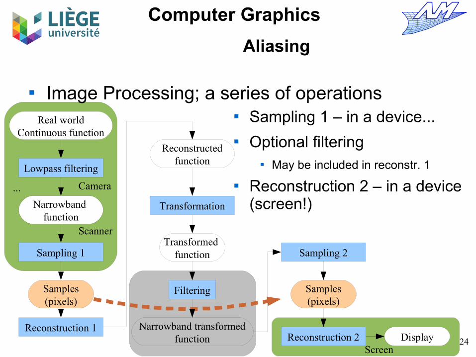
Image Processing; a series of operations
Sampling 1
Reconstruction 1
Sampling 2
Reconstruction 2
Lowpass filtering
Real worldContinuous function
Samples(pixels)
Narrowband function
Samples(pixels)
DisplayScreen
Scanner
Camera...
Sampling 1 – in a device... Optional filtering
May be included in reconstr. 1
Reconstruction 2 – in a device (screen!)
Filtering
Narrowband transformedfunction
Transformation
Reconstructedfunction
Transformed function
25
Computer Graphics
Aliasing
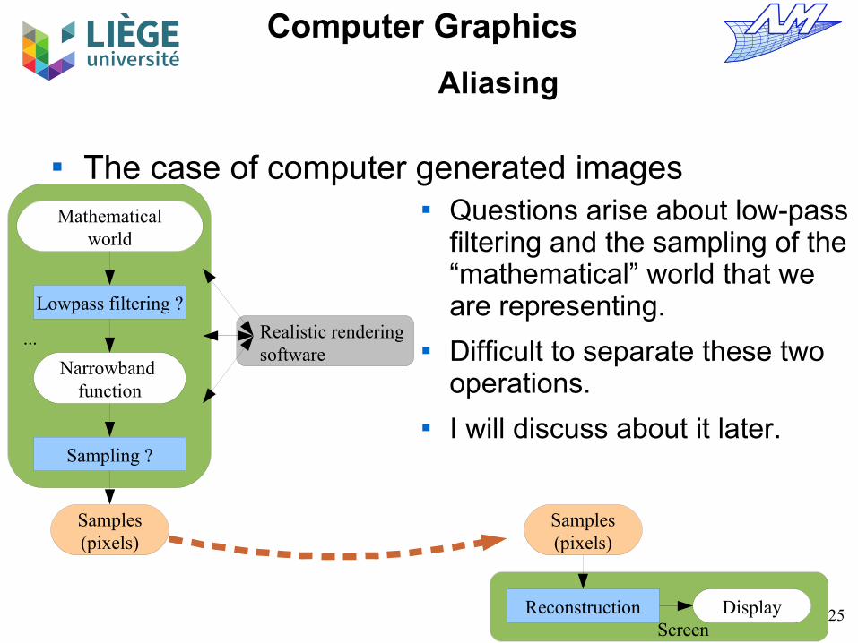
The case of computer generated images
Sampling ?
Reconstruction
Lowpass filtering ?
Mathematicalworld
Samples(pixels)
Narrowband function
Samples(pixels)
DisplayScreen
Realistic rendering software
...
Questions arise about low-pass filtering and the sampling of the “mathematical” world that we are representing.
Difficult to separate these two operations.
I will discuss about it later.

26
Computer Graphics
Aliasing
J. Blinn's Corner

27
Computer Graphics
Aliasing
Convolution
f∗g t = ∫−∞
∞
f t− g d

28
Computer Graphics
Aliasing
Reconstruction From samples Convolution with a certain function
Linear, bicubic, Gaussian, etc... Interpolates the signal where it no longer exists (between samples) Back to a continuous signal ...
29
Computer Graphics
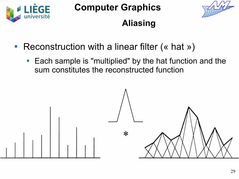
Aliasing
Reconstruction with a linear filter (« hat ») Each sample is "multiplied" by the hat function and the
sum constitutes the reconstructed function
*
30
Computer Graphics
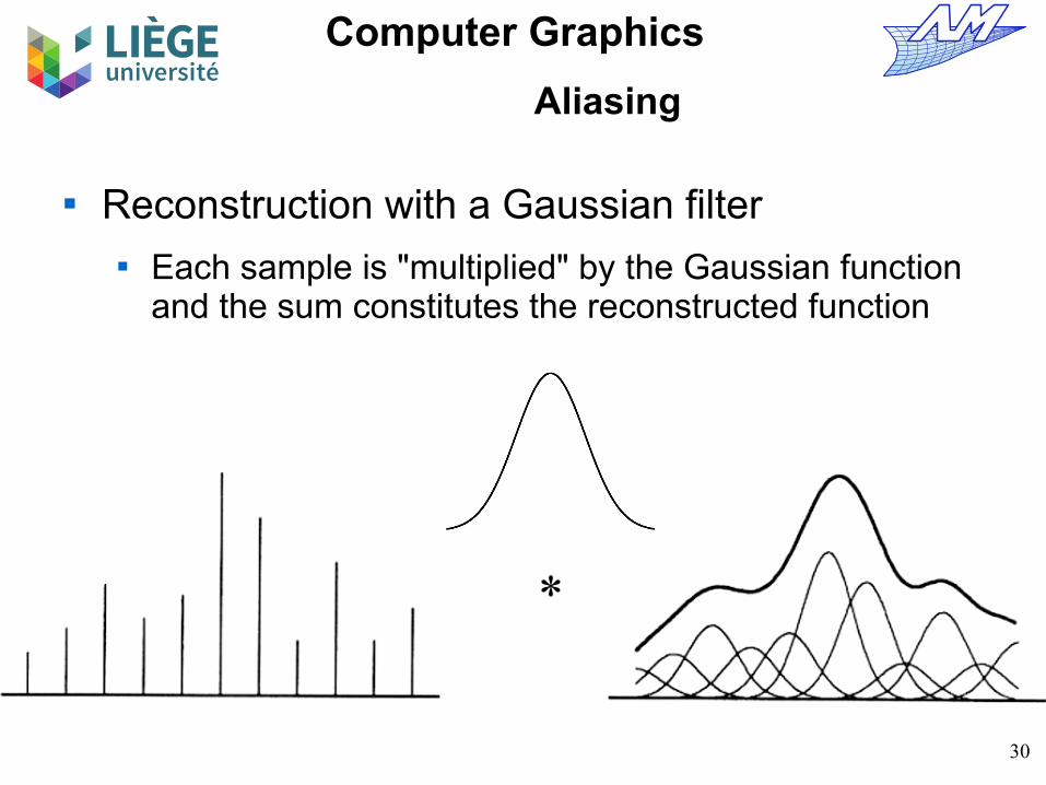
Aliasing
Reconstruction with a Gaussian filter Each sample is "multiplied" by the Gaussian function
and the sum constitutes the reconstructed function
*

31
Computer Graphics
Aliasing
Reconstruction with sinc Convolution with a cardinal sine that has an infinite
support : provided that the original signal meets the Shannon condition, the exact original signal is reconstructed !
*
sinc x=sin x x
32
Computer Graphics
Aliasing
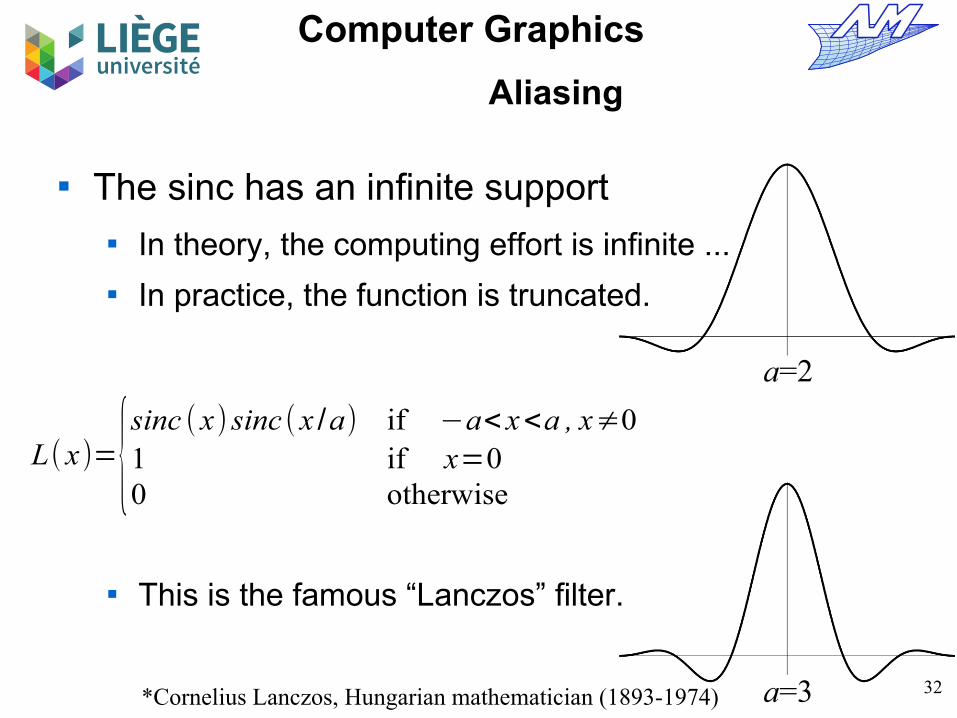
The sinc has an infinite support In theory, the computing effort is infinite ... In practice, the function is truncated.
This is the famous “Lanczos” filter.
L( x)={sinc (x) sinc (x /a) if −a< x<a , x≠01 if x=00 otherwise
a=2
a=3*Cornelius Lanczos, Hungarian mathematician (1893-1974)

33
Computer Graphics
Aliasing
Bicubic interpolation
Nearest neighborinterpolation
Bilinear interpolation
34
Computer Graphics
Aliasing
Transformation Change the position of the image / or the samples
Rotation Scaling Etc...
In cases where the targeted sample density is lower, filtering with a low-pass filter is needed before resampling
In cases where the targeted sample density is identical or finer, a simple resampling after reconstruction is sufficient
35
Computer Graphics
Aliasing
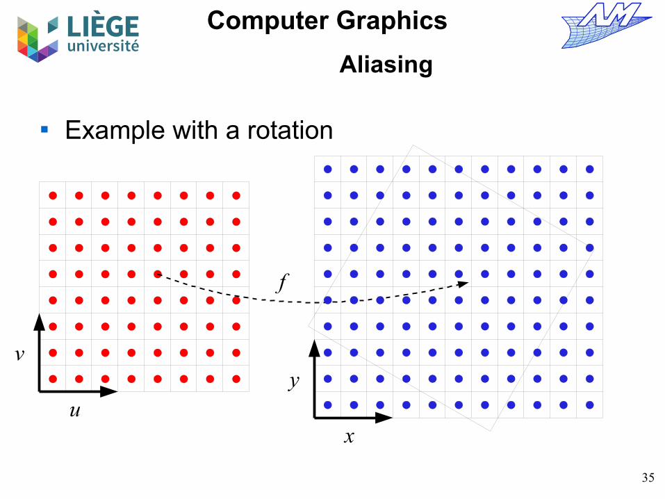
Example with a rotation
u
v
x
y
f

36
Computer Graphics
Aliasing
Direct mapping – bad idea
u
v
x
y
f
Several source samples in the destination pixel
No source sample in the destination pixel
Loop on source image...but difficult to “reconstruct” the target image (it is an inverse problem)

37
Computer Graphics
Aliasing
Inverse mapping
u
v
x
y
f-1
Loop on pixels of the target image ...
- Resampling is unavoidable- A reconstruction of the source image is used here

38
Computer Graphics
Aliasing
The reconstruction is crucial to the quality of the target image Nearest neighbour – lots of aliasing Bilinear – not much aliasing but blurred image (loss of
details) Bicubic and « Lanczos » - better (but more
computationally expensive)

39
Computer Graphics
Aliasing
Nearest neighboor :
u
v

40
Computer Graphics
Aliasing
Serie of 36 rotations of 5° → 180° followed by a mirroring (without any loss) Original images magnified 10x

41
Computer Graphics
Aliasing
« Nearest neighbour » filter

42
Computer Graphics
Aliasing
Bilinear :
u
v
f u ,v = f 0,01−u1−v f 1,0u 1−v f 0,11−uv
f 1,1uv
f 0,1
f 1,0f 0,0
f 1,1
u=u−umin
umax−umin
v=v−v min
vmax−vmin
f u ,v

43
Computer Graphics
Aliasing
« Bilinear » filter
44
Computer Graphics
Aliasing
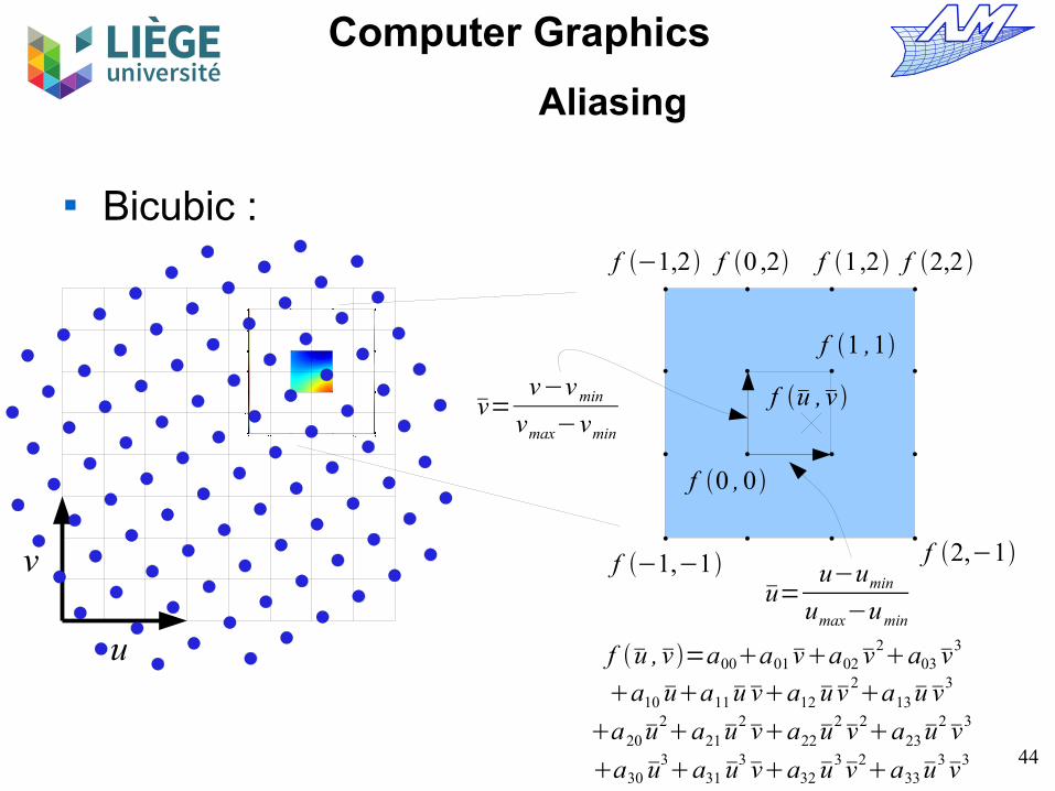
Bicubic :
u
v
f −1,2
f 2,−1f −1,−1
f 2,2
v=v−v min
vmax−vmin
f u ,v
f 0 ,2 f 1,2
f 1 ,1
f u ,v =a00a01va02v2a03v
3
a10 ua11uva12 uv2a13uv
3
a20u2a21u
2va22u
2v
2a23u
2v
3
a30 u3a31 u
3va32 u
3v
2a33u
3v
3
u=u−umin
umax−umin
f 0 , 0
45
Computer Graphics
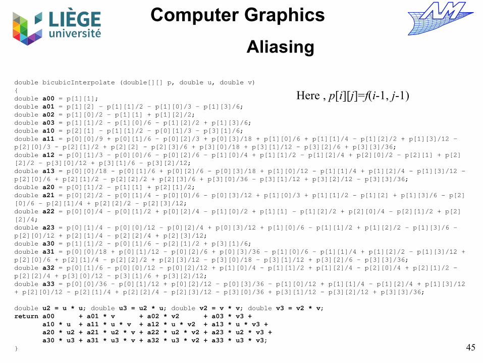
double bicubicInterpolate (double[][] p, double u, double v){double a00 = p[1][1];double a01 = p[1][2] - p[1][1]/2 - p[1][0]/3 - p[1][3]/6;double a02 = p[1][0]/2 - p[1][1] + p[1][2]/2;double a03 = p[1][1]/2 - p[1][0]/6 - p[1][2]/2 + p[1][3]/6;double a10 = p[2][1] - p[1][1]/2 - p[0][1]/3 - p[3][1]/6;double a11 = p[0][0]/9 + p[0][1]/6 - p[0][2]/3 + p[0][3]/18 + p[1][0]/6 + p[1][1]/4 - p[1][2]/2 + p[1][3]/12 - p[2][0]/3 - p[2][1]/2 + p[2][2] - p[2][3]/6 + p[3][0]/18 + p[3][1]/12 - p[3][2]/6 + p[3][3]/36;double a12 = p[0][1]/3 - p[0][0]/6 - p[0][2]/6 - p[1][0]/4 + p[1][1]/2 - p[1][2]/4 + p[2][0]/2 - p[2][1] + p[2][2]/2 - p[3][0]/12 + p[3][1]/6 - p[3][2]/12;double a13 = p[0][0]/18 - p[0][1]/6 + p[0][2]/6 - p[0][3]/18 + p[1][0]/12 - p[1][1]/4 + p[1][2]/4 - p[1][3]/12 - p[2][0]/6 + p[2][1]/2 - p[2][2]/2 + p[2][3]/6 + p[3][0]/36 - p[3][1]/12 + p[3][2]/12 - p[3][3]/36;double a20 = p[0][1]/2 - p[1][1] + p[2][1]/2;double a21 = p[0][2]/2 - p[0][1]/4 - p[0][0]/6 - p[0][3]/12 + p[1][0]/3 + p[1][1]/2 - p[1][2] + p[1][3]/6 - p[2][0]/6 - p[2][1]/4 + p[2][2]/2 - p[2][3]/12;double a22 = p[0][0]/4 - p[0][1]/2 + p[0][2]/4 - p[1][0]/2 + p[1][1] - p[1][2]/2 + p[2][0]/4 - p[2][1]/2 + p[2][2]/4;double a23 = p[0][1]/4 - p[0][0]/12 - p[0][2]/4 + p[0][3]/12 + p[1][0]/6 - p[1][1]/2 + p[1][2]/2 - p[1][3]/6 - p[2][0]/12 + p[2][1]/4 - p[2][2]/4 + p[2][3]/12;double a30 = p[1][1]/2 - p[0][1]/6 - p[2][1]/2 + p[3][1]/6;double a31 = p[0][0]/18 + p[0][1]/12 - p[0][2]/6 + p[0][3]/36 - p[1][0]/6 - p[1][1]/4 + p[1][2]/2 - p[1][3]/12 + p[2][0]/6 + p[2][1]/4 - p[2][2]/2 + p[2][3]/12 - p[3][0]/18 - p[3][1]/12 + p[3][2]/6 - p[3][3]/36;double a32 = p[0][1]/6 - p[0][0]/12 - p[0][2]/12 + p[1][0]/4 - p[1][1]/2 + p[1][2]/4 - p[2][0]/4 + p[2][1]/2 - p[2][2]/4 + p[3][0]/12 - p[3][1]/6 + p[3][2]/12;double a33 = p[0][0]/36 - p[0][1]/12 + p[0][2]/12 - p[0][3]/36 - p[1][0]/12 + p[1][1]/4 - p[1][2]/4 + p[1][3]/12 + p[2][0]/12 - p[2][1]/4 + p[2][2]/4 - p[2][3]/12 - p[3][0]/36 + p[3][1]/12 - p[3][2]/12 + p[3][3]/36;
double u2 = u * u; double u3 = u2 * u; double v2 = v * v; double v3 = v2 * v;return a00 + a01 * v + a02 * v2 + a03 * v3 + a10 * u + a11 * u * v + a12 * u * v2 + a13 * u * v3 + a20 * u2 + a21 * u2 * v + a22 * u2 * v2 + a23 * u2 * v3 + a30 * u3 + a31 * u3 * v + a32 * u3 * v2 + a33 * u3 * v3;}
Aliasing
Here , p[i][j]=f(i-1, j-1)
46
Computer Graphics
Aliasing
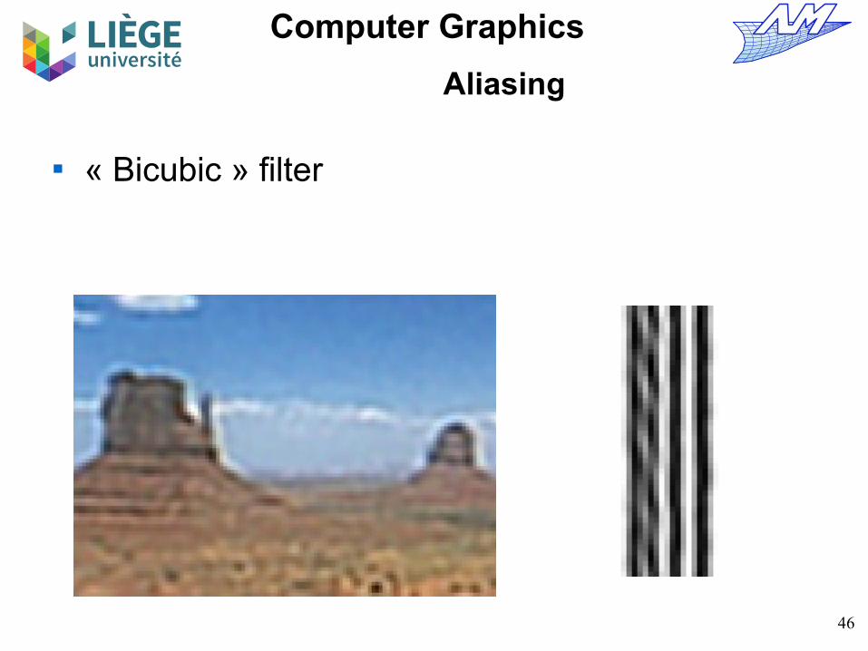
« Bicubic » filter
47
Computer Graphics
Aliasing
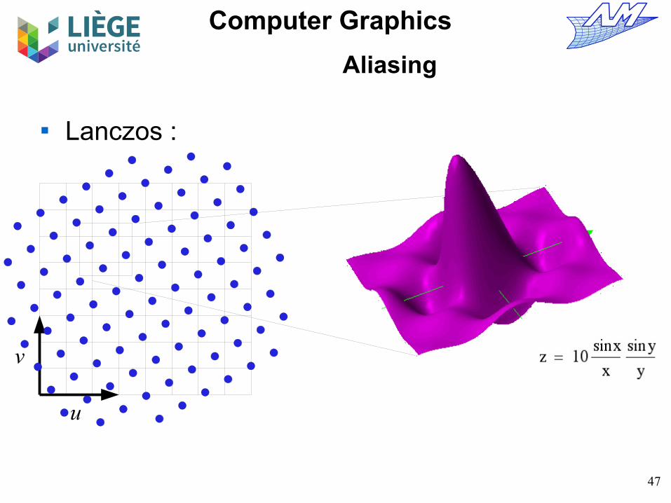
Lanczos :
u
v

48
Computer Graphics
Aliasing
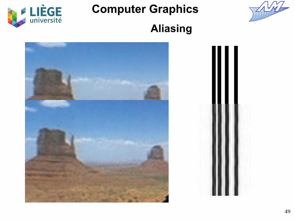
« Lanczos » filter
49
Computer Graphics
Aliasing

50
Computer Graphics
Aliasing
Without antialiasingnearest neighbour
Antialiasingby oversampling 4and simple average
Antialiasing by Lanczos filtering(ideal but costly)
Another example

51
Computer Graphics
Aliasing
Case of downsampling
u
v
The input data must be filtered with a low pass filter, that is matchedwith the resolution of the destination image

52
Computer Graphics
Image storage
53
Computer Graphics
Image storage
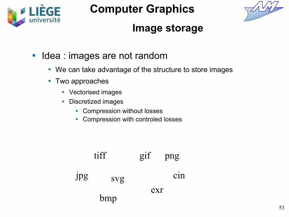
Idea : images are not random We can take advantage of the structure to store images Two approaches
Vectorised images Discretized images
Compression without losses Compression with controled losses
jpg
tiff gif png
svg
bmpexr
cin

54
Computer Graphics
Image storage
TIFF : universal format but sometimes partially implemented JPG : limited to 8bits/channel, DCT compression with losses
(WWW) PNG : open format, 1/2/4/8 indexed bits, 8/16 bits/channel ; alpha
channel (transparency), LZW type compression – no patent (WWW) GIF : indexed 8 bits, transparency (1 bit), LZW type compression,
possible animation, expired patent (WWW) SVG : vector images CIN : old format « cineon » 10 bits / channel, used for special
effects. Lossless compression EXR : open format Lucasfilm (ILM): 16/32 bits by channel in floating
point, lossless compression BMP : old Windows format without compression limited to 8 bits by
channel + transparency

55
Computer Graphics
Image storage
How to choose ? Outline drawing, to be scaled --- vector format Images in general, sampled (bitmap) format
56
Computer Graphics
Image storage
Vector images Generally no “geometric” compression A typical example : character fonts destined to be
enlarged Ideal as a format for line drawings
WMF : windows metafile (exclusively windows)
SVG : Scalable vector graphics (open standard)
+ proprietary formats : coreldraw, adobe illustrator...
DXF : for technical drawings (Autocad)

57
Computer Graphics
Image storage
Bitmap images Uncompressed storage
BMP (old), TIFF (1/8/16 bits/c, floating point) , PNG (8,16 bits/c, alpha channel,1,2,4,8 bits indexed col.), PNG (indexed colors + alpha channel), EXR (floating point 16,32 bits/channel)
Lossless compression TIFF, PNG, GIF, EXR
Lossy compression TIFF, JPG(8 bits), JPEG2000 (improved JPG but not used due to
patents !)
58
Computer Graphics
Image storage
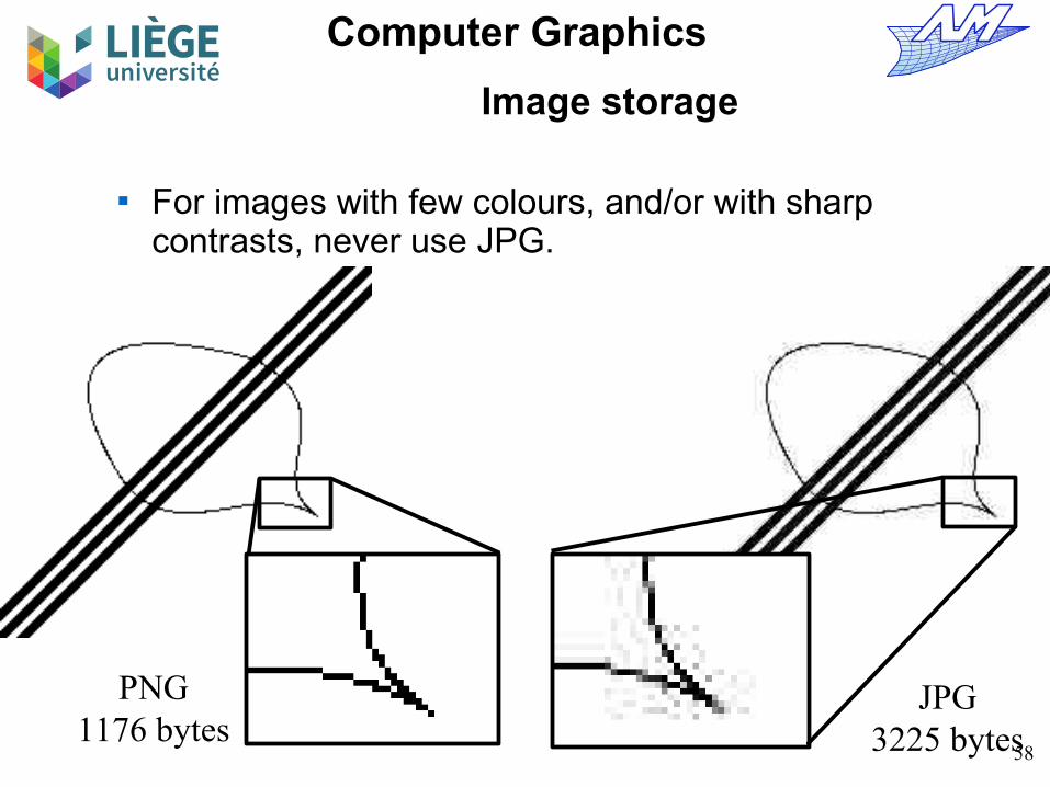
For images with few colours, and/or with sharp contrasts, never use JPG.
PNG1176 bytes
JPG3225 bytes

59
Computer Graphics
Image storage
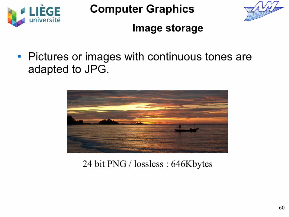
Pictures or images with continuous tones are adapted to JPG.
24 bit JPG : 85Kbytes
60
Computer Graphics
Image storage
Pictures or images with continuous tones are adapted to JPG.
24 bit PNG / lossless : 646Kbytes

61
Computer Graphics
Image storage
Pictures or images with continuous tones are adapted to JPG.
8 bit PNG (256 indexed colours) : 227 Kbytes

62
Computer Graphics
Image storage
Pictures or images with continuous tones are adapted to JPG.
4 bit - PNG (16 indexed colours) : 108 Kbytes
63
Computer Graphics
Image storage
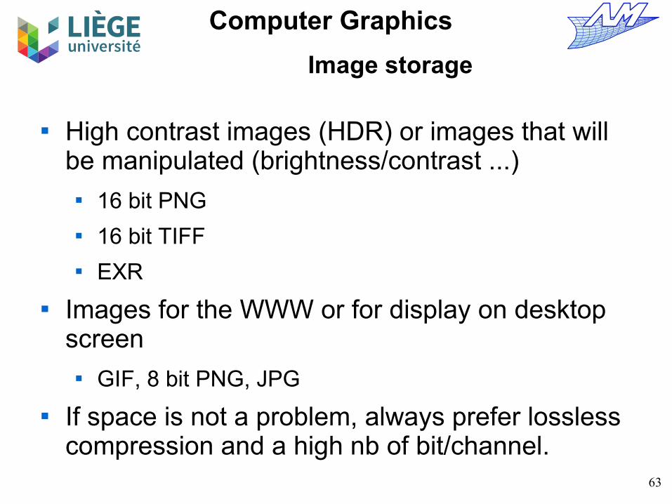
High contrast images (HDR) or images that will be manipulated (brightness/contrast ...) 16 bit PNG 16 bit TIFF EXR
Images for the WWW or for display on desktop screen GIF, 8 bit PNG, JPG
If space is not a problem, always prefer lossless compression and a high nb of bit/channel.

64
Computer Graphics
Image storage
There is no universal image format !
65
Computer Graphics
Perspective and transformation matrices

66
Computer Graphics
Perspective
« Classical » projections
Plane projections
Parallel Perspective
Orthogonal Oblique 1vanishing point
3 vanishingpoints
Multiview Axonometric
2 vanishing points

67
Computer Graphics
PerspectivePerspective (central) projection
Parallel projection
AxonometricOrthogonal
Oblique projection

68
Computer Graphics
Perspective
Vanishing points in perspective projection
69
Computer Graphics
Perspective

70
Computer Graphics
Perspective
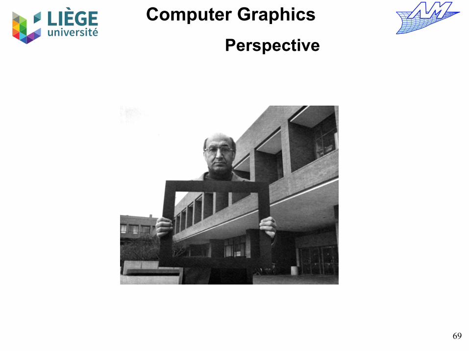
The perspective is a fairly accurate representation of what the eye sees Based on central projection In first approximation, the eye (or a camera) is made
of a lens (the eye's lens), and a projection plane of the image (retina). The lens may be considered as a point in what follows.
SA
A'
P f

71
Computer Graphics
Perspective
Equivalent configuration used in computer graphics
SAA'
fP

72
Computer Graphics
Perspective
Parallel projection is the limiting case where f tends to infinity.
S AA'
f P

73
Computer Graphics
Geometric transformations

74
Computer Graphics
Transformation matrices
Geometric transformations Two goals
Get from 3D coordinates objects a projection on the screen plane (coordinates 2D + depth details)
From elementary objects, they can be placed anywhere in the volume, optionally modified by operations such as shearing or scaling.
75
Computer Graphics
Affine transformations
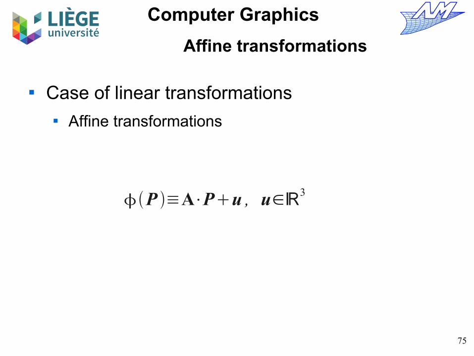
Case of linear transformations Affine transformations
P ≡A⋅Pu , u∈ℝ3

76
Computer Graphics
identity : u = 0, A = I , I is the identitymatrice,
translation :u is the translation vector, A = I,
scaling u = 0, A is a diagonal matrice, whose terms define the scalesalong the axes,
rotation : u = 0, A is the rotation matrice,
Some affine transformations
u=0 ; A=[cos −sin 0sin cos 0
0 0 1]
u=0 ; A=[a 0 00 b 00 0 c ]
u=[abc ] ; A=[
1 0 00 1 00 0 1 ]
u=0 ; A=[1 0 00 1 00 0 1 ]
77
Computer Graphics
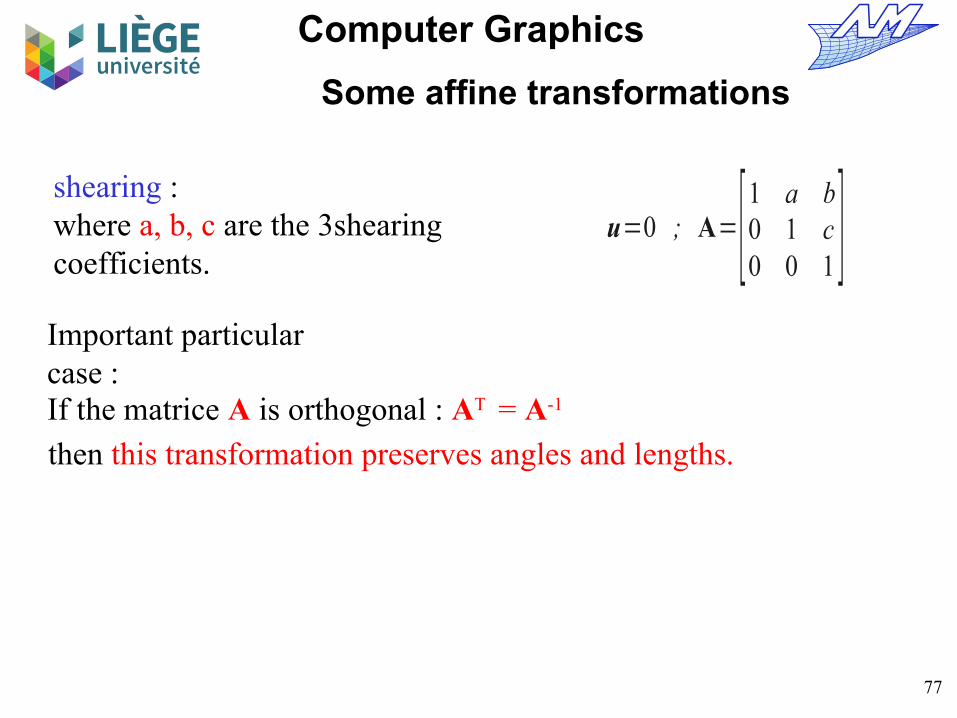
shearing :where a, b, c are the 3shearing coefficients.
u=0 ; A=[1 a b0 1 c0 0 1 ]
Some affine transformations
If the matrice A is orthogonal : AT = A-1
Important particular case :
then this transformation preserves angles and lengths.

78
Computer Graphics
Additive treatment for the translation
The treatment is not the same for all operations ...
Matrix treatment
P1=S⋅P0
P1=R⋅P0
P1=C⋅P0
P1=P0t
Multiplicative treatment
79
Computer Graphics
Homogeneous coordinates
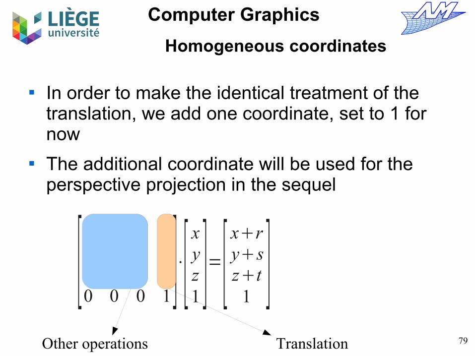
In order to make the identical treatment of the translation, we add one coordinate, set to 1 for now
The additional coordinate will be used for the perspective projection in the sequel
[1 0 0 r0 1 0 s0 0 1 t0 0 0 1
]⋅[xyz1]=[
xryszt
1]
TranslationOther operations

80
Computer Graphics
- translation :
- scaling :
Transformation matrices
D t =[1 0 0 u0 1 0 v0 0 1 w0 0 0 1
] ; t=[uvw1]
S p , q , r =[p 0 0 00 q 0 00 0 r 00 0 0 1
]
81
Computer Graphics
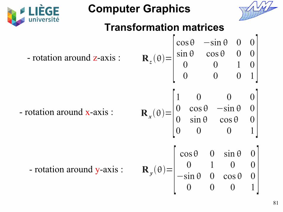
- rotation around x-axis :
- rotation around z-axis :
- rotation around y-axis :
R z =[cos −sin 0 0sin cos 0 0
0 0 1 00 0 0 1
]R x =[
1 0 0 00 cos −sin 00 sin cos 00 0 0 1
]R y =[
cos 0 sin 00 1 0 0
−sin 0 cos 00 0 0 1
]
Transformation matrices
82
Computer Graphics
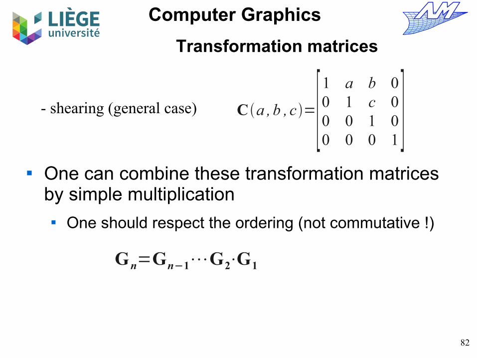
- shearing (general case) Ca , b , c=[1 a b 00 1 c 00 0 1 00 0 0 1
]Transformation matrices
One can combine these transformation matrices by simple multiplication One should respect the ordering (not commutative !)
Gn=Gn−1⋯G2⋅G1
83
Computer Graphics
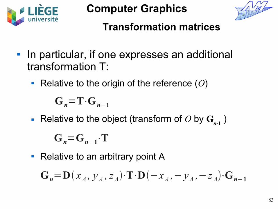
Transformation matrices
In particular, if one expresses an additional transformation T: Relative to the origin of the reference (O)
Relative to the object (transform of O by Gn-1
)
Relative to an arbitrary point A
Gn=T⋅Gn−1
Gn=Gn−1⋅T
Gn=D x A , y A , zA⋅T⋅D−x A ,− yA ,− z A⋅Gn−1
84
Computer Graphics
Transformation matrices
Change of reference (for parallel projections) 3D global reference to reference 2D screen 12 parameters in the transformation We can specify the transformation uniquely by 4
points (forming a tetrahedron) and their transforms

85
Computer Graphics
0
1
2
33D
2D (or 3D)
P 0=[0 1 0 00 0 1 00 0 0 11 1 1 1
]
Transformation matrices
P 1=[x0 x1 x2 x3
y0 y1 y2 y3
z0 z1 z2 z3
1 1 1 1]
T=P1⋅P0−1
P 1=T⋅P0
z x
y
y'
x'z'
O
O'
86
Computer Graphics
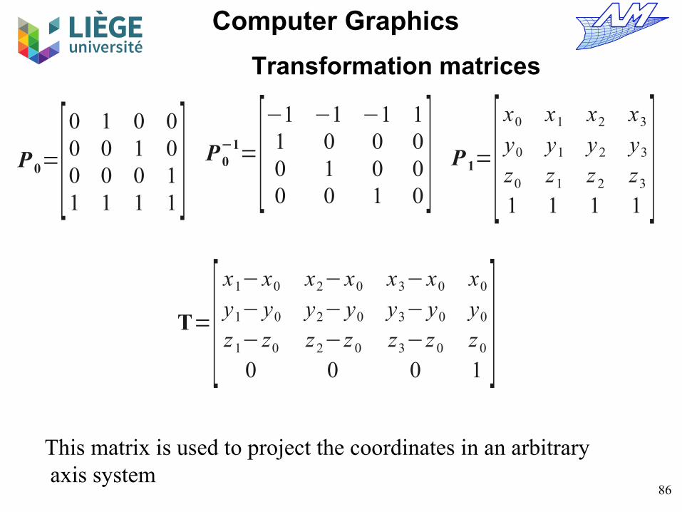
Transformation matrices
This matrix is used to project the coordinates in an arbitrary axis system
P 0=[0 1 0 00 0 1 00 0 0 11 1 1 1
] P 0−1=[−1 −1 −1 11 0 0 00 1 0 00 0 1 0
] P 1=[x0 x1 x2 x3
y0 y1 y2 y3
z0 z1 z2 z3
1 1 1 1]
T=[x1−x0 x2−x0 x3−x0 x0
y1− y0 y2− y0 y3− y0 y0
z1−z0 z2−z0 z3−z0 z0
0 0 0 1]

87
Computer Graphics
Transformation matrices
Using the transformations that we have just seen , we can :
- Transform space coordinates (x, y, z) coordinates to screen coordinates (x ', y', z '= depth), expressing the position in space of the view associated with the screen
- Consider a scale factor to adjust the size of the virtual screen space and switch from (x', y') to (i, j) which is the geometrical position on the screen
The third coordinate (depth z') will be used to compute hidden faces.

88
Computer Graphics
Transformation matrices
For points where the 4th (homogenous) coordinate w is different from one We consider that all points situated along a line going
through the origin are equivalent This corresponds to a central projection on the
hyperplane w = 1; the following points are (geomtrically) equivalent:
If w = 0, it means a vector in homogeneous coordinates
There is a way to distinguish vectors and points !
[wx , wy ,wz , w ]⇔[ x , y , z ,1]
[ x , y , z ,0]

89
Computer Graphics
Transformation matrices
Perspective transformation We will consider a special case that does not betray
the generality of the approach P is at the origin O of the reference frame The screen is a plane of normal n=(0,0,1) (perpendicular to z),
containing P We look towards the positive z.
AA'
d
z
y x
P(0,0,0)
S(0,0,-d)
Q(x,y,z)
Q'(x',y',z')
x '
x=
y '
y=
dd z
z'=0

90
Computer Graphics
Transformation matrices
Screen coordinates in function of space coordinates
We will change that so that the 3rd coordinate is going through the same scaling
z'=0
x'=
x
1 zd
y '=
y
1 zd
z'=
z
1 zd
x'=
x
1 zd
y '=
y
1 zd

91
Computer Graphics
Transformation matrices
The three Cartesian coordinates
may be expressed differently in the homogeneous space (via the equivalence relation) :
x'=
x
1 zd
y '=
y
1 zd
z'=
z
1 zd
x
1zd
, y
1zd
, z
1zd
,1≡x , y , z ,1 zd
92
Computer Graphics
Transformation matrices
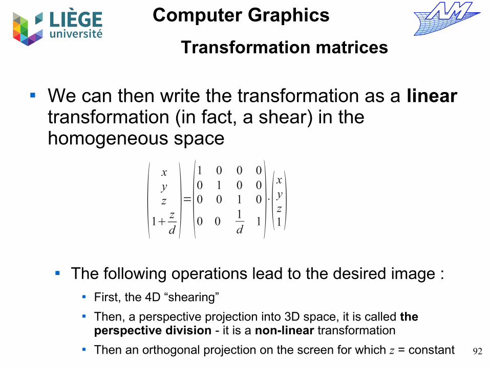
We can then write the transformation as a linear transformation (in fact, a shear) in the homogeneous space
The following operations lead to the desired image : First, the 4D “shearing” Then, a perspective projection into 3D space, it is called the
perspective division - it is a non-linear transformation Then an orthogonal projection on the screen for which z = constant
xyz
1zd=
1 0 0 00 1 0 00 0 1 0
0 0 1d
1 ⋅xyz1

93
Computer Graphics
Transformation matrices
Field of view and effective construction of transformation matrices Canonical view field
Screen : consists in pixels, centred at the origin, in the plane
Transformation of the canonical field to the screen coordinates
x c , yc , zc∈[−1,1 ]3
n x , n y
x
y
xz x p
y p
z p
1=
nx
20 0
n x−12
0ny
20
n y−1
20 0 1 00 0 0 1
M s
⋅xc
yc
zc
1
sight
x p , y p∈[−0.5 , n x−0.5 ]×[−0.5 , n y−0.5 ]
NB : If yc is reversed, it must be taken into account ...
94
Computer Graphics
(l,b,f)
(-1,-1,-1)
Transformation matrices
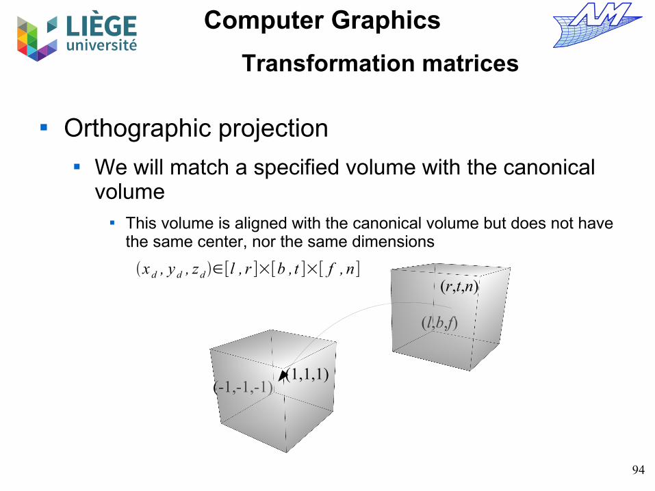
Orthographic projection We will match a specified volume with the canonical
volume This volume is aligned with the canonical volume but does not have
the same center, nor the same dimensions
x d , y d , zd ∈[l , r ]×[b ,t ]×[ f , n]
(1,1,1)
(r,t,n)

95
Computer Graphics
Transformation matrices
The process resorts to a translation followed by a dilation.
xc
yc
zc
1=
2r−l
0 0 0
02
t−b0 0
0 02
n− f0
0 0 0 1⋅
1 0 0 −rl
2
0 1 0 −bt
2
0 0 1 −n f
20 0 0 1
M c
⋅xd
yd
z d
1
fn b
t

96
Computer Graphics
Transformation matrices
Viewpoints with an arbitrary position and orientation One would like to watch in an arbitrary direction and
from any point The position of the eye (o), the view direction (r) and “noon” -local
vertical line for the observer- (m) are defined An orthonormal (o, u, v, w) frame is constructed from the data.
x
y
xzr
mo
w v
u
w=−r∥r∥
u=−m×w∥m×w∥
v=w×u

97
Computer Graphics
Transformation matrices
The alignment of the space coordinates with those of the viewer is done with two changes Translation bringing the coordinates of the eye to the
origin Rotation about the axes to align them with the global
axes
xd
y d
zd
1=
xu yu zu 0xv yv z v 0xw yw zw 00 0 0 1
⋅1 0 0 −x o
0 1 0 −yo
0 0 1 −zo
0 0 0 1
M v
⋅xe
ye
ze
1
98
Computer Graphics
Transformation matrices
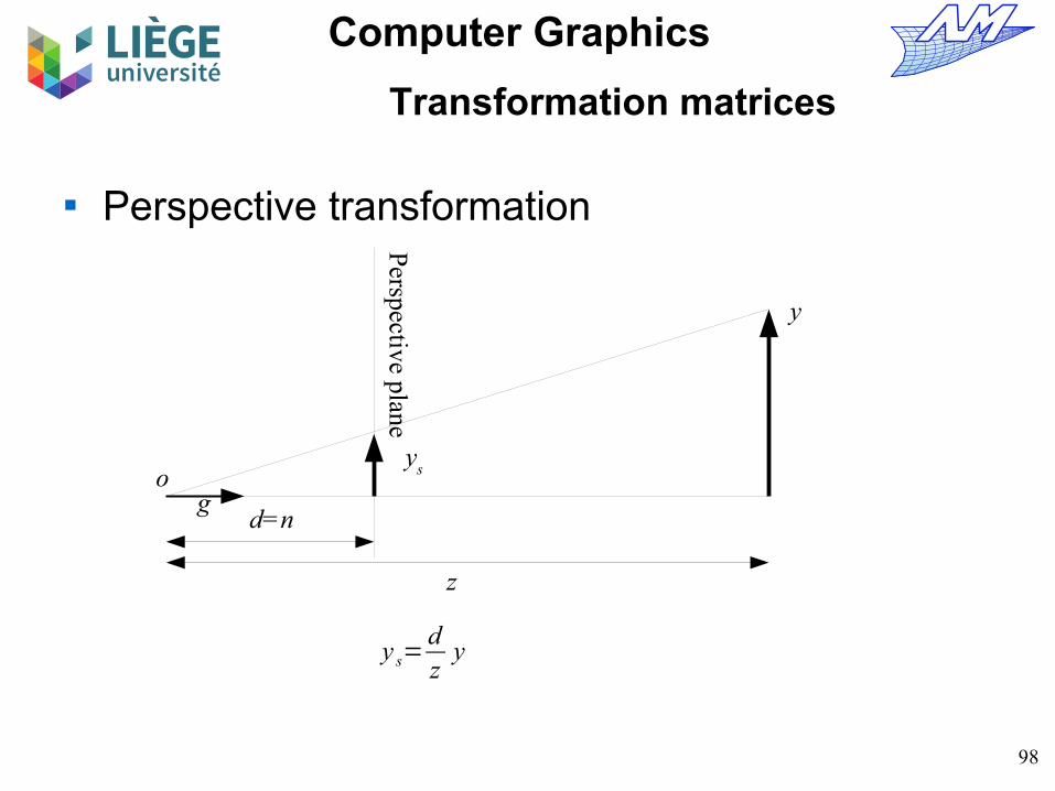
Perspective transformation
og
z
d=n
y
Perspective plane
ys
y s=dz
y
99
Computer Graphics
Transformation matrices
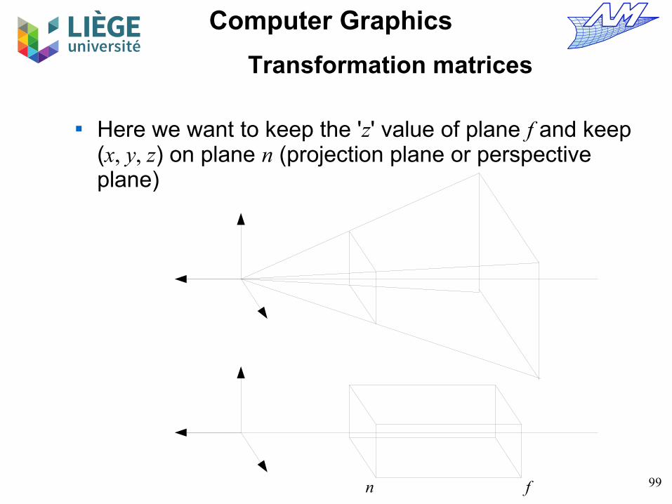
n f
Here we want to keep the 'z' value of plane f and keep (x, y, z) on plane n (projection plane or perspective plane)

100
Computer Graphics
Transformation matrices
To use homogeneous coordinates, All three components must be divided by the same
value Recall what we saw before :
Compared to this matrix, it has a displacement to bring the eye to (0,0,0) , thus keeping z=n unchanged
And a small change to keep the points z = f unchanged as well
xyz
1zd=
1 0 0 00 1 0 00 0 1 0
0 0 1d
1 ⋅xyz1
101
Computer Graphics
Transformation matrices
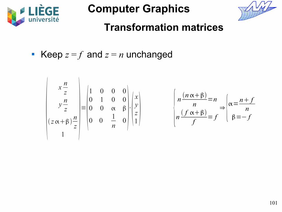
Keep z = f and z = n unchanged
x
nz
ynz
znz
1≡
1 0 0 00 1 0 00 0
0 0 1n
0 ⋅xyz1 {
nn
n=n
n f
f= f⇒ {=
n fn
=− f
102
Computer Graphics
Transformation matrices
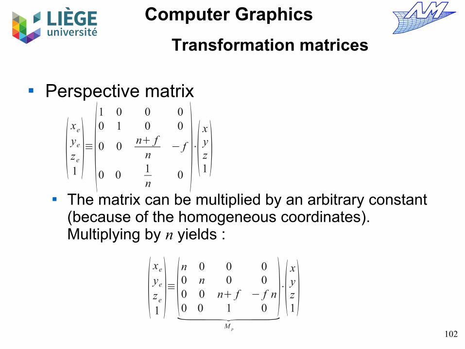
Perspective matrix
The matrix can be multiplied by an arbitrary constant (because of the homogeneous coordinates). Multiplying by n yields :
xe
ye
ze
1≡
1 0 0 00 1 0 0
0 0 n fn
− f
0 0 1n
0 ⋅xyz1
xe
ye
ze
1≡
n 0 0 00 n 0 00 0 n f − f n0 0 1 0
M p
⋅xyz1

103
Computer Graphics
Transformation matrices
The perspective matrix that we have just defined suppose one looks in the direction of the negative z We must therefore apply it after the change of point of
view ! The complete chain of transformations is therefore :
M=M s⋅M c⋅M p⋅M v

104
Computer Graphics
Transformation matrices
In particular, the matrix
is called perspective projection matrix, and allows to reach from the real space the canonical volume [-1,1]3
M proj _ persp=M c⋅M p=2 nr−l
0lrl−r
0
02 n
t−bbtb−t
0
0 0f nn− f
2 f nf −n
0 0 1 0
z=−∣ f∣ zc=−1
z=−∣n∣ zc=1M=M s⋅M proj _ persp⋅M v
Depends on the hardware Depends on the type of projection Depends on your point of view

105
Computer Graphics
Transformation matrices
OpenGL...
"Mathematical" convention used in this course
OpenGL convention
106
Computer Graphics
Transformation matrices
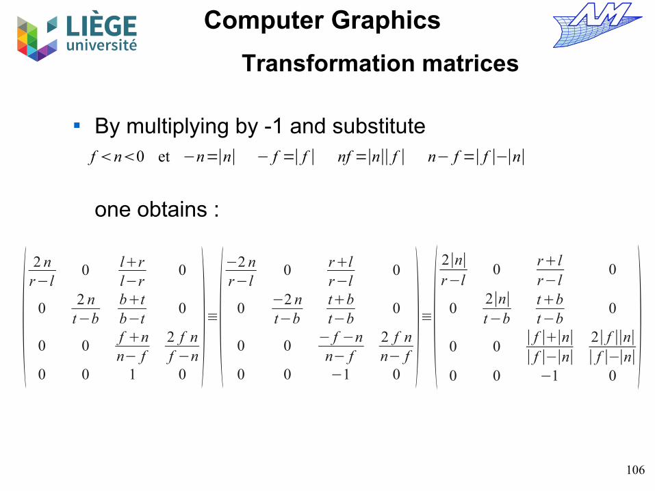
By multiplying by -1 and substitute
one obtains :
2 n
r−l0 lr
l−r0
02 n
t−bbtb−t
0
0 0f nn− f
2 f nf −n
0 0 1 0≡−2 nr−l
0 rlr−l
0
0−2 nt−b
tbt−b
0
0 0− f −nn− f
2 f nn− f
0 0 −1 0≡
2∣n∣r−l
0rlr−l
0
02∣n∣t−b
tbt−b
0
0 0∣ f ∣∣n∣∣ f ∣−∣n∣
2∣ f ∣∣n∣∣ f ∣−∣n∣
0 0 −1 0
f n0 et −n=∣n∣ − f =∣ f ∣ nf =∣n∣∣ f ∣ n− f =∣ f ∣−∣n∣
107
Computer Graphics
Transformation matrices
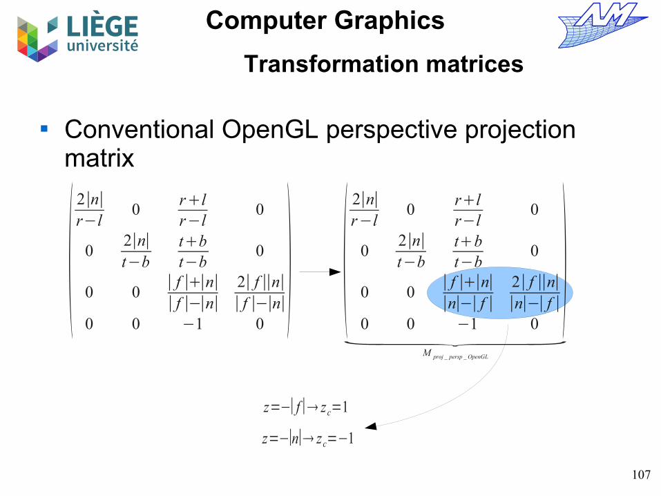
Conventional OpenGL perspective projection matrix
2∣n∣r−l
0rlr−l
0
02∣n∣t−b
tbt−b
0
0 0∣ f ∣∣n∣∣ f ∣−∣n∣
2∣ f ∣∣n∣∣ f ∣−∣n∣
0 0 −1 0
2∣n∣r−l
0rlr−l
0
02∣n∣t−b
tbt−b
0
0 0∣ f ∣∣n∣∣n∣−∣ f ∣
2∣ f ∣∣n∣∣n∣−∣ f ∣
0 0 −1 0
M proj _ persp _ OpenGL
z=−∣ f∣ zc=1
z=−∣n∣ zc=−1

108
Computer Graphics
Transformation matrices
Idem without perspective transformation
2
r−l0 0 0
02
t−b0 0
0 02
n− f0
0 0 0 1⋅
1 0 0 −rl
2
0 1 0 −bt
2
0 0 1 −n f
20 0 0 1
M c
=2
r−l0 0
lrl−r
02
t−b0
btb−t
0 02
n− ff nf −n
0 0 0 1
M proj _ orth
109
Computer Graphics
Transformation matrices
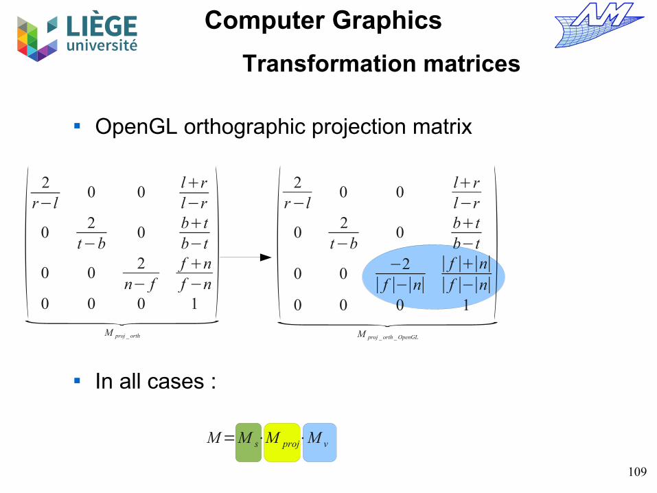
OpenGL orthographic projection matrix
In all cases :
2
r−l0 0
lrl−r
02
t−b0
btb−t
0 02
n− ff nf −n
0 0 0 1
M proj _ orth
2
r−l0 0
lrl−r
02
t−b0
btb−t
0 0−2∣ f ∣−∣n∣
∣ f ∣∣n∣∣ f ∣−∣n∣
0 0 0 1
M proj _ orth _ OpenGL
M=M s⋅M proj⋅M v
110
Computer Graphics
Transformation matrices
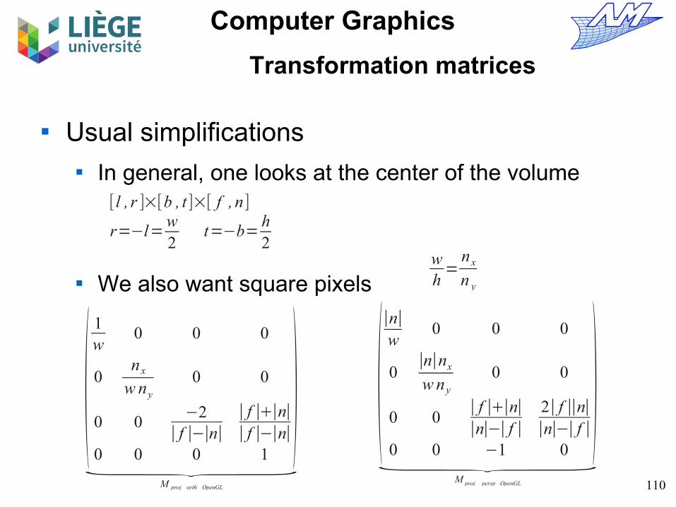
Usual simplifications In general, one looks at the center of the volume
We also want square pixels
[ l , r ]×[b , t ]×[ f , n]
r=−l=w2
t=−b=h2
wh=
n x
n y
1w
0 0 0
0n x
w ny
0 0
0 0−2∣ f ∣−∣n∣
∣ f ∣∣n∣∣ f ∣−∣n∣
0 0 0 1
M proj _ orth _ OpenGL
∣n∣w
0 0 0
0∣n∣nx
w n y
0 0
0 0∣ f ∣∣n∣∣n∣−∣ f ∣
2∣ f ∣∣n∣∣n∣−∣ f ∣
0 0 −1 0
M proj _ persp _OpenGL

111
Computer Graphics
Transformation matrices
One can also specify the field of view (obviously for perspective projections only)
tan =w∣n∣⇒w=∣n∣tan
1
tan0 0 0
0nx
n y tan 0 0
0 0∣ f ∣∣n∣∣n∣−∣ f ∣
2∣ f ∣∣n∣∣n∣−∣ f ∣
0 0 −1 0
M proj _ persp _ OpenGL

112
Computer Graphics
Transformation matrices
Exercise Compute the transformation matrix for an observer located at (x =
10, y = 10, z = 10) facing the direction (-1, -1, -1). A vector from the vertical plane is the vector (0,1,0). The screen is 1000 by 1000 pixels.
Angle of view : 45° (tan 45 = 1) Plane position n and f : z=10 and z=20 respectively
w=−g∥g∥ u=−
t×w∥t×w∥
v=w×u
xu yu zu 0xv yv zv 0xw yw z w 00 0 0 1
⋅1 0 0 −xo
0 1 0 − yo
0 0 1 −z o
0 0 0 1
M v
2∣n∣r−l
0rlr−l
0
02∣n∣t−b
tbt−b
0
0 0∣ f ∣∣n∣∣n∣−∣ f ∣
2∣ f ∣∣n∣∣n∣−∣ f ∣
0 0 −1 0
M proj _ persp _ OpenGL
(n x
20 0
n x−12
0n y
20
n y−1
20 0 1 00 0 0 1
)⏟
M s
113
Computer Graphics
Transformation matrices
How to select (point at an object with the mouse and pick the object) Using the reverse transformation Need to know for each pixel, the geometric primitive
recently drawn We'll see how later...

114
Computer Graphics
Two paradigms for synthetic image generation

115
Computer Graphics
2 paradigms...
A projection of the objects on the plane of the screen Purely geometrical aspects
Using transformation matrices Need for hidden line removal algorithm « Clipping » and « culling » techniques
Allows to draw only visible entities (and minimizing side effects)
Colouring / shadowing Lighting Textures Laws of reflection
Possibility of real-time graphics (e.g. videogames, ...) OpenGL type implementation (in hardware)
116
Computer Graphics
2 paradigms...
Projective “à la OpenGL” paradigm Start from the objects and their coordinates in space Determine at each point or every facet, lighting
features, textures, etc ... Project into the coordinate space of the screen
Transformation matrices seen before
Draw the object in discrete form Raster algorithm - (!) aliasing hidden faces ! The colour of each pixel is determined by the information calculated
above (previously interpolated or computed on-the-fly)

117
Computer Graphics
2 paradigms...
Ray-tracing paradigm Geometric aspects
We start form pixels to meet objects Finding the intersection of a ray and objects (usually triangulated)
Problem of the hidden faces : automatically solved ! Culling is useful (to avoid unnecessary searches)
Colouring Realistic reflection laws Realistic lighting law Complex textures
Relatively slow but higher fidelity Easy introduction of new light/texture models

118
Computer Graphics
2 paradigms...
Ray-tracing paradigm Start from screen pixels Draw a line through the eye and that pixel and
calculate the intersection with the first object encountered online Particular case if the surface is a dielectric or metal (smooth metal or
glass, liquid etc ...) : the ray is reflected, or deflected or both
Determine the color of the object at this point Use of physical or empirical laws Consider the light - and shadows
Give the determined pixel color (!) again, problems of potential aliasing !
119
Computer Graphics
2 paradigms...
Common issues for both techniques Laws of light-surface interaction, reflection, types of
surfaces Textures Geometrical modelling Meshes Colour theory Aliasing
120
Computer Graphics
2 paradigms...
Specific topics to ray-tracing Radiosity equation Calculation of shadows Refraction, reflection Use of Computational Geometry to lower the
computation costs

121
Computer Graphics
2 paradigms...
Specific issues to the projective approach Visibility problems (clipping and hidden faces) Raster algorithms

122
Computer Graphics
2 paradigms...
There are hybrid approaches Allows to combine the advantages of both paradigms
Speed (projective approach) Fidelity (ray tracing approach) They are more or less close to a very versatile implementation in
software of the more rigid OpenGL stack.
E.g. Pixar Renderman.

123
Computer Graphics
Project

124
Computer Graphics
Project
Available topics A) Homemade Ray Tracer
Upgrade an existing ray-tracing program (which I provide) Programming & Implementation
B) Topic of your choice If you want to work on a topic that interests you and is within the
scope of the course (I have to validate early enough !)
125
Computer Graphics
Project
Project guidlines Individual project Deliverables
(A) Homemade Ray Tracer a) “Specifications” : definition of what you will do (+ who) , planning ... b) Final report detailing the philosophy of your contribution (why and
how) + code + results and critical analysis + detailed personal contributions if you are two
c) Small presentation to show the results

126
Computer Graphics
Project
(B) Own topic a) Definition of the topic (originality, interest, context ...) b) “Specifications” : definition of what you will do (+ who) , planning ... c) Final report detailing the philosophy of your contribution (why and
how) + code + results and critical analysis + detailed personal contributions if you are two
d) Small presentation to show the results
Physical limits of the documents Specifications : 1-2 A4 pages Final report : max 15 A4 pages Definition of the subject (B) : 1 A4 page

127
Computer Graphics
Project
Deadlines Choice of subjects : Feb 27th
In the case C) definition of the subject : Feb 27th
Specifications and planning : March 13th Submission of reports : before June 1st Relative weight in the final mark : TBD
128
Computer Graphics
Project
Homemade Ray-tracer Canvas available on the course's website
http://www.cgeo.ulg.ac.be/infographie
Developed in portable C ++ under Linux Uses OpenGL and FLTK
I do not want you develop a significant GUI for what you're doing (takes too long) - simply implement models of reflection, shadows, geometry etc ... and test this directly in the code (in the main() function for example). GUI might be an option when everything else works.
There are (very) few comments ... You are allowed to modify the existing code...

129
Computer Graphics
Project
Subjects related to the HomeMade RayTracer
1 – Implement subsurface scattering Rendering of semi-transparent objects (e.g. skin)
2 – Interfacing with an existing solid modeler CATIA files, Solidworks, etc.
3 – Metropolis algorithm Unbiased physical rendering
4 – Efficient ray intersection with smooth CAD surfaces bézier/NURBS surfaces and the like
All – Gather all ! Keep in mind that you work together...part of the evaluation depends
on the integration of all developments in the same source tree.