Introduction: Humidity and Climate Change · PDF fileimplications for how temperature changes may occur aloft. ... _____ Ch. 1 Introduction: Humidity and Climate Change

______________________________Ch. 1 Introduction: Humidity and Climate Change

___________________________________________________________________ 1

Chapter 1

Introduction: Humidity and

Climate Change

1.1 INTRODUCTION - RATIONALE

The climate system of the Earth is ever changing across all space and time scales.

Evidence for past changes arises from “proxies” such as ice cores and geological

records, and for more recent times from tree rings, coral growth, and historical

documentary records. Only over the last two Centuries have we been actively measuring

the atmosphere. Since the late 18th

Century, measurements by thermometers and other

surface instruments on land have been available along with measurements made by

ships. After the Second World War, balloon-based sounding of the free atmosphere

began and finally, since the 1970s satellites have also been employed to monitor the

climate system.

Most of our modern measurement systems have been employed primarily for weather

forecasting purposes. Little thought has been given as to whether we can compare

present observations to data from a century or even a decade previously. The result has

been changes in instrumentation and practice which, whilst likely improving the

absolute accuracy of the measurement, also compromise the historical continuity of the

record for long-term climate monitoring purposes. To create a climate data record

requires the identification and removal of as many such non-climatic influences as

possible (homogenisation) to yield an estimate of the true climate evolution.

To date, climate data record construction efforts have principally considered

temperature and to a lesser extent pressure and precipitation. However, even taken

together these are an incomplete diagnostic of the climate system and do not adequately

constrain our understanding. Humidity, both relative and absolute, is potentially a very


___________________________________________________________________ 2

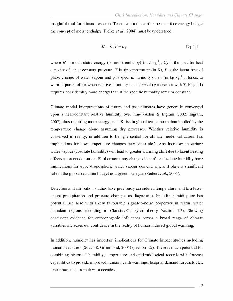
insightful tool for climate research. To constrain the earth‘s near-surface energy budget

the concept of moist enthalpy (Pielke et al., 2004) must be understood:

qLTCH p += Eq. 1.1

where H is moist static energy (or moist enthalpy) (in J kg-1

), Cp is the specific heat

capacity of air at constant pressure, T is air temperature (in K), L is the latent heat of

phase change of water vapour and q is specific humidity of air (in kg kg-1

). Hence, to

warm a parcel of air when relative humidity is conserved (q increases with T, Fig. 1.1)

requires considerably more energy than if the specific humidity remains constant.

Climate model interpretations of future and past climates have generally converged

upon a near-constant relative humidity over time (Allen & Ingram, 2002; Ingram,

2002), thus requiring more energy per 1 K rise in global temperature than implied by the

temperature change alone assuming dry processes. Whether relative humidity is

conserved in reality, in addition to being essential for climate model validation, has

implications for how temperature changes may occur aloft. Any increases in surface

water vapour (absolute humidity) will lead to greater warming aloft due to latent heating

effects upon condensation. Furthermore, any changes in surface absolute humidity have

implications for upper-tropospheric water vapour content, where it plays a significant

role in the global radiation budget as a greenhouse gas (Soden et al., 2005).

Detection and attribution studies have previously considered temperature, and to a lesser

extent precipitation and pressure changes, as diagnostics. Specific humidity too has

potential use here with likely favourable signal-to-noise properties in warm, water

abundant regions according to Clausius-Clapeyron theory (section 1.2). Showing

consistent evidence for anthropogenic influences across a broad range of climate

variables increases our confidence in the reality of human-induced global warming.

In addition, humidity has important implications for Climate Impact studies including

human heat stress (Souch & Grimmond, 2004) (section 1.2). There is much potential for

combining historical humidity, temperature and epidemiological records with forecast

capabilities to provide improved human health warnings, hospital demand forecasts etc.,

over timescales from days to decades.


___________________________________________________________________ 3

To date, efforts to collate records of surface water vapour to form climate records have:

been limited to small regions; considered only land observations; or made no attempt to

ensure station homogeneity. Therefore, this thesis aims to create a truly global

homogenous humidity dataset suitable for use in climate studies. Alongside efforts

underway elsewhere to create and maintain upper-air humidity datasets from

radiosondes (McCarthy et al., 2005) and satellites (Soden et al., 2005; Jackson et al.,

2006; RSS (Remote Sensing Systems - http://www.remss.com/); Wagner et al., 2006),

this provides potential to constrain our understanding of recent changes in both

temperature and humidity throughout the troposphere.

1.2 THE ROLE OF WATER VAPOUR IN THE ATMOSPHERE

Water vapour plays a key role in determining the dynamical and radiative properties of

the climate system (Elliott, 1995; Allen & Ingram, 2002; Trenberth et al., 2005). Water

vapour and its transport around the atmosphere is a fundamental component of the

hydrological cycle. It also modifies the radiative balance, being a naturally occurring

greenhouse gas. These features are indicated pictorially in Fig. 1.2 (a much simplified

diagram). The Clausius-Clapeyron relation yields exponential increases in the

atmosphere’s water holding capacity with increasing T at approximately 7 % K-1

(Manabe & Wetherald, 1967; Allen & Ingram, 2002; Trenberth et al., 2005) (Fig. 1.1).

For rising T and in the presence of unlimited water supplies (e.g. over the oceans) it can

be expected that actual moisture content (i.e. specific humidity (q)) will also increase,

thus maintaining a reasonably constant relative humidity (RH) (Trenberth, 1999). Where

moisture is limiting (e.g. over many land areas), q should increase less thereby allowing

temperatures to increase by higher amounts and RH to decrease. It is generally assumed

that RH distributions remain constant in the atmosphere over long time scales and this

has been an emergent constraint on which the climate models have converged at all

latitudes (Allen & Ingram, 2002). However, this premise remains unproven in the

observational record as to date no truly climate-quality global humidity dataset has been

available.

The hydrological cycle is thought to be enhanced both in terms of weather system and

precipitation intensity as higher air temperatures enable greater take up and transfer of

water vapour (latent heat) from the surface to the upper atmosphere (Folland et al.,

2001b; Groisman et al., 2004; Trenberth et al., 2005). Latent heat transfer is a major


___________________________________________________________________ 4

driver for atmospheric dynamics, including: the formation and propagation of mesoscale

and synoptic scale weather systems; atmospheric circulation; and flooding and drought

events (Elliott, 1995). Atmospheric circulation is mainly forced by latent heat release in

the tropics and radiative cooling in the polar regions (Arpe, 1991; Sohn et al., 2004),

giving us the more predictable modes of climate (air mass formation regions, seasonal

weather characteristics, ENSO (El Niño Southern Oscillation) etc.) that regionally

people have learned to live with or even come to depend upon. Exactly how these

climate features might be affected by changes in surface humidity is an important

question. The record 2005 North Atlantic hurricane season, in terms of intensity and

heavy rainfall, has been linked by some to higher sea-surface temperature (SST) and

associated increases in water vapour where resulting latent heat release is a driver for

hurricanes (Trenberth & Shea, 2006; Anthes et al., 2006; Santer et al., 2006).

Water vapour affects the earth’s energy budget in four main ways. Firstly, water vapour

stores energy in the form of latent heat. This is released into the atmosphere during

condensation and precipitation. Secondly, as a gas it affects the energy budget through

long-wave radiation effects (Fig. 1.2). Indeed, it is by far the largest and the most

significant of the greenhouse gases (Elliott, 1995; Harries, 1997; Kiehl & Trenberth,

1997), which collectively facilitate a positive feedback mechanism which at present

maintains the Earth’s energy budget and cycle in a habitable state. Without these

greenhouse gases, our planet’s equilibrium T would lie around -18 oC rather than 14

oC

(global mean surface T) (Ahrens, 2000; Jones et al., 1999). Thirdly, water vapour is the

source for clouds which have significant and complex radiative properties depending on

their height, optical properties and latitude (Zhang et al., 1995; Kiehl & Trenberth,

1997; Philipona & Dürr, 2004). Finally, as discussed earlier, the amount of moisture in

the air determines the energy required to change the T of that air (moist enthalpy -

Pielke et al., 2004).

Water vapour as a greenhouse gas is part of a major positive feedback loop (Cess, 1989;

Elliott, 1995; Zhang et al., 1995), increasing climate sensitivity by a factor of two

(Manabe & Wetherald, 1967; Sohn & Schmetz, 2004; Stephens et al., 2004; Bony et al.,

2006). Notably, this long-wave radiation trapping is at its maximum in the mid- to

upper-troposphere, despite the vertical water vapour profile which is greatest at the

surface reducing rapidly with height (Held & Soden, 2000). As water vapour can be

transported vertically through convection and subsidence, and horizontally by


___________________________________________________________________ 5

atmospheric circulation, changes in surface absolute moisture can effect changes in

moisture aloft (McCarthy & Toumi, 2004).

An increase in atmospheric moisture provides more condensate for cloud formation.

However, this and cloud development depends on many other factors such as

atmospheric T, RH, stability, circulation and availability of condensation nuclei.

Observed changes have been found in cloud amount, height and optical properties such

as depth, liquid water content and opacity (Cess et al., 2003; Trenberth et al., 2005;

Bony et al., 2006) which will in turn affect radiation and thus impact on climate. These

can effect a net cooling or a net warming through interaction with both short-wave and

long-wave radiation (Fig. 1.2). This depends on latitude, altitude and optical properties

(Stephens and Greenwald 1991; Zhang et al. 1995; Philipona & Dürr, 2004; Trenberth

et al., 2005). Additionally, the quantity of atmospheric water vapour directly interacts

with radiation prior to cloud interaction thus further complicating cloud feedbacks

(Groisman et al., 2000; Sun et al., 2000). The presentday net radiative effect of clouds is

thought to be close to zero. However, cloud feedback depends on so many factors that it

is uncertain as to whether climate change may impact short-wave and long-wave

radiation differentially (Bony et al., 2006). As such, cloud feedbacks are the key source

of uncertainty in climate models (Trenberth et al., 2005; Webb et al., 2006).

Of more direct societal interest, surface humidity has a compound effect on human

comfort in terms of heat stress (Levzey & Tinker, 1996). High humidity in terms of RH,

inhibits evaporation, making cooling by perspiration less effective (Souch &

Grimmond, 2004) contributing to higher heat-stress and potential mortality than would

otherwise be expected (Davis et al., 2002; Changnon et al., 2003). However, low RH

too can be a source of heat stress, particularly through dryness enhancing the effect of

air pollution (Diaz et al., 2002a, 2002b). Generally, temperatures and humidities outside

of the usually accustomed range pose a human health threat (Souch & Grimmond, 2004;

McGregor, G. pers. comm.). A change in amount or distribution of surface water vapour

can thus be linked to direct human health impacts.

Surface humidity may be affected by factors other than rising temperatures. These

include: changes in atmospheric circulation (possibly brought about by changes in

climate); changes in land-use including irrigation and reservoirs; and increasing air-

traffic although this is essentially an upper-tropospheric effect (Lee, 1991; Elliott, 1995;


___________________________________________________________________ 6

Schwartzman et al., 1998; Gaffen & Ross, 1999; Changnon et al., 2003; Marquart et al.,

2003).

Clearly, water vapour has played and will continue to play a key role in our changing

climate as: a much affected variable; a major agent of change; and a human health issue.

However, more research is urgently needed to quantify and understand recent changes,

their causes, and their impacts fully.

1.3 MEASURING SURFACE HUMIDITY

Station observed humidity is commonly measured as one of: wet-bulb temperature (Tw);

dewpoint temperature (Tdw); or RH. Other humidity variables can then be calculated

through empirically based conversions from any of these observed parameters with the

inclusion of pressure (P) and air T (dry-bulb temperatures) where necessary (Chapter 2).

There are a wide variety of instruments, collectively called hygrometers, available to

measure each of the above variables. The following discussion is by no means

exhaustive.

The most commonly reported surface measure, Tw, is usually obtained using a

psychrometer which contains both a dry-bulb and wet-bulb thermometer. Under suitably

aspirated conditions, the contact of a hydrated wick (by means of a reservoir) around the

wet-bulb thermometer causes evaporative cooling of the wet-bulb relative to the dry-

bulb. The quantity of this depression relative to the dry-bulb temperature is directly

related to the level of saturation of the air. Aspiration of the thermometer may be done:

manually, by whirling the psychrometer through the air (Sling Psychrometer);

mechanically, by means of a fan (Assman Psychrometer); or naturally, by situating the

psychrometer in a ventilated box (often a Stevenson Screen) with adequate exposure to

allow air-flow though.

Instruments to measure RH most commonly use either capacitance or resistance of an

electrical current. For example, the Dewcel calculates RH from changes in the

conductivity of lithium chloride as it absorbs/evaporates moisture from/to the

surrounding air, requiring adequate ventilation. It can also measure Tdw. Chilled mirror

hygrometers measure Tdw directly by cooling the mirror to the temperature at which

moisture forms.


___________________________________________________________________ 7

All instruments have potential for error. Wet-bulb thermometers can be affected by:

both under- and over-ventilation depending on the Screen location; the presence of the

observer which can cause positive errors in both T and Tw; and by heat conduction from

dry parts of the thermometer depending on the stem length (Folland, 1977). In sub-zero

temperatures where an ice-bulb calculation is used to convert to other humidity

variables (section 2.1), the wick around the bulb may not actually be frozen and so

small positive errors may occur (Simidchiev, 1986). Furthermore, the Stevenson Screen

or wick around the wet-bulb may freeze preventing ventilation of the wet-bulb (icing)

(Makkonnen & Laakso, 2005; van Wijngaarden & Vincent, 2005). The wet-bulb

reservoir may freeze or in warm conditions evaporate completely, causing the wick

around the wet-bulb thermometer to dry out. Icing and reservoir freezing were found to

be particular problems for automatic stations in Canada, if instruments were not

checked regularly (Déry & Stieglitz, 2002). By implication this is likely a problem at

other high latitude stations. Reservoir evaporation is a common problem even in

temperate conditions. The 2003-2004 Global Climate Observing System (GCOS)

plastic screen trial at three British stations had to discount 13 % of psychrometer

measurements because the wet-bulb had dried out (Elms & Hatton, 2005). All of these

problems, in effect, inhibit evaporation, and thus inhibit depression of Tw relative to T

giving erroneously high (frequently 100%) RH recordings and a moist bias to the data.

Automated stations, which are increasingly common (http://www.faa.gov/asos/hist-

aos.htm), are especially prone to such problems where stations are unmanned for long

periods.

Retarded response of RH sensors, which increases as T decreases (Elms & Hatton,

2005; Simidchiev, 1986) is also a problem, as is potential dripping of condensation

down the sensor probe. The latter can be avoided by situating the RH sensor with the

probe pointing skywards, as recommended by the manufacturer. However, to keep the

sensor close to the dry-bulb thermometer and avoid the effect of any temperature

gradient within the Screen, it is common practice to place the sensor technically upside

down.

Further sources of error occur when the humidity record is physically observed as one

variable but converted to and reported as another. The algorithms chosen for such

conversions are not standardised and vary often between stations and even within one


___________________________________________________________________ 8

station over time. The error introduced from such conversions is discussed further in

section 2.6.

Over land there is little in the way of metadata (data providing information about the

station, instrument and observing practices) and so statistical methods must be utilised

to detect and adjust for artificial discontinuities in individual station records

(homogenisation). However, where available this metadata can prove useful. For

example, the change over from psychrometer to Dewcel, widespread in Canadian

stations, produced a negative step in RH at a number of stations (van Wijngaarden &

Vincent, 2005). Outside of the US and north-west Europe, available metadata for land

stations is sparse to non-existent. Even for these regions there are no comprehensive,

easily accessible, repositories of high quality, electronically available (necessary for use

with very large datasets) metadata at the time of undertaking this thesis. Therefore, there

is a large degree of ambiguity in how to assign and adjust for breakpoints leading to

differences in results depending upon the exact methodology applied (structural

uncertainty - Thorne et al. (2005a)). For marine data there exists an electronic record of

metadata from 1955 for observing ships (http://icoads.noaa.gov/metadata/) which lists

information about instrument type and exposure (including height) for each year. While

this aids identification of inhomogeneities and adjustment quantification, some

structural uncertainty may still exist due to inevitable subjectivity of decision making

regarding error adjustments and bias corrections.

1.4 THE PHYSICAL RELATIONSHIPS BETWEEN HUMIDITY

VARIABLES OF INTEREST

Atmospheric water vapour is a complex meteorological element. For atmospheric

studies at the surface it can be described in numerous ways, the most common of these

being: RH; e; saturated vapour pressure (es); q; Tdw; and Tw (WMO, 1996; McIlveen,

1998) (Table 1.1). All except q can be measured directly.

The chosen humidity variables for this project are e, q and RH. These are selected

because: they represent an absolute, proportional and a relative (respectively) measure

of humidity; they are highly suitable for climate studies; they are represented in climate

models (q and RH); and because they are comparable with other studies both at the


___________________________________________________________________ 9

surface (New et al., 2000; Gaffen & Ross, 1999; van Wijngaarden & Vincent, 2005;

Dai, 2006) and in the upper air (McCarthy & Toumi, 2004).

Vapour pressure is the partial pressure of water vapour as an atmospheric gas. It is

measured in mb or hPa. Within the earth’s atmosphere, water vapour behaves as an

ideal gas, satisfying the following conditions:

VP /1∝ at constant T Eq. 1.2

TV ∝ at constant P Eq. 1.3

TP ∝ at constant V Eq. 1.4

where V is volume in m3. It can thus be described by water vapour density (ρv) in kg m

-3

using the equation of state:

TRe vvρ= Eq. 1.5

where Rv is the specific gas constant for water vapour (462 J K-1

kg-1

) (McIlveen, 1998).

Specific humidity is the proportion of the mass of water vapour to the total mass of

moist air. It is measured in g kg-1

or kg kg-1

and can be described thus:

dv

v

mm

mq

+= Eq. 1.6

where mv is the mass of water vapour in kg and md is the mass of dry air in kg. It can

also be described in terms of density because the water vapour and the moist air occupy

the same total volume:

ρ

ρ vq = Eq. 1.7

where ρ is the density of the moist air (kg m-3

). If each density is then replaced by the

appropriate equation of state this gives:

vPR

eRq = Eq. 1.8

where R is the specific gas constant for moist air (which can be substituted with the dry

air value 287 J K-1

kg-1

without causing serious error). The ratio of the gas constants

R/Rv is the inverse ratio of the molecular weights of each and can be substituted with

0.622 (known as ε). Thus q can be derived from e as follows:


___________________________________________________________________ 10

P

eq

ε= Eq. 1.9

where e and P are both either in mb or hPa, and q is output in kg kg-1

(McIlveen, 1998).

Importantly, e recorded at T is by definition the same as es at the simultaneous Tdw

(es(Tdw)). The saturation vapour pressure is the partial pressure of water vapour on a

parcel of air should that parcel become saturated at its current T (es (T)), essentially a

measure of the water holding capacity of the air. The saturation specific humidity (qs) is

the equivalent for q. From this knowledge of both the actual moisture content of the air

and potential moisture content of the air (at saturation), the relative humidity, which

refers to the extent of saturation of the air as a percentage, can be calculated (McIlveen,

1998):

( )( )

=

Te

TeRH

s

dws100 Eq. 1.10

which can be rewritten:

=

se

eRH 100 Eq. 1.11

1.5 RECENTLY OBSERVED CLIMATE CHANGES

1.5.1 Recent Changes in Atmospheric Humidity at the Surface

To date there have been few observational surface humidity studies. Those of note are

described in detail in Table 1.2 along with abbreviations which will be used henceforth.

All but DAI, ISSM and WOR are regionally focussed and most end before 2000. None

are truly global (land and marine) homogenised humidity datasets. Without such testing

and adjustment (where necessary) a dataset is arguably not suitable for climate research

as the possibility that any apparent trends in the data result from non-climatic origin

cannot be ignored. Homogenisation (see section 3.3.1 for a full discussion), while

unlikely to remove all non-climatic discontinuities in the data, produces a dataset that as

a reflection of actual climate changes, is far more robust. While six out of the ten

datasets described make efforts to detect inhomogeneities, most simply remove any

suspect stations and only one (WG) makes any attempt to adjust the data.


___________________________________________________________________ 11

The range of quality control varies widely between datasets. GR, ROB, VWV and SSR

require stations with a certain length of record or minimum missing data requirements.

Only DAI and GR document checking the physical plausibility of each variable (e.g.

Tdw >-80 o, <60

oC and ≤ T), although this may have been undertaken by the institutions

that collect and provide the data originally. Six datasets incorporate an outlier test of

some form. No dataset makes any attempt to remove humidity specific errors such as

wick drying or icing (section 1.3).

The primary data sources are not entirely independent between each dataset as can be

seen in Table 1.2. However, differences in quality control tests, period of record, station

coverage, trend fitting method and dataset construction approach, the latter of which is

referred to as structural uncertainty (Thorne et al., 2005a), can be expected to lead to

discrepancies between datasets.

Given the lack of homogenisation, and ad-hoc quality control applied, it can be argued

that none of the datasets discussed here are truly climate quality. HadCRUH will

incorporate all the above quality control tests, undergo homogenisation, have near-

global coverage and at some point in the future be updateable, thus improving on any

humidity dataset available to the climate community to date.

According to these studies, over the US, there was an overall picture of moistening both

annually (since 1951 - ROB, since 1961- GR and since 1975 - NEW and DAI) with

significant positive trends found in q, Tdw and e over most regions except Hawaii (GR).

DAI showed statistically significant positive trends in regionally averaged q (0.1 g kg-1

10yr-1

). Similarly, GR (1961-1995) showed significant moistening (q and Tdw) in all

seasons except Autumn, but the longer, earlier record period of ROB (1951-1990) while

concordant with positive trends in Spring, showed drying trends in Winter (not

significance tested). For RH, DAI found mostly positive and significant (0-2 % 10yr-1

)

trends in RH whereas although GR found some evidence of increases, especially at

night and during Winter (Alaska and High Plains) and Spring (south-west and south-

central), trends were not generally statistically significant nor spatially consistent. DAI

found little of significance over much of Alaska but the earlier analysis of GR found

large positive trends (significant at the 0.01 confidence level) in all seasons except

Autumn. Clearly there are some discrepancies between the datasets, likely due to the

reasons discussed above. GR investigated sources of potential inhomogeneity but did


___________________________________________________________________ 12

not make any adjustments. They also looked into sources of the water vapour increase

and discounted changes in instrumentation and fossil fuel burning emission of water

vapour (too small). They cited irrigation as a potential local contributing factor in some

regions.

Trends in q and e over Canada from 1975 were predominantly positive and significant

(NEW; DAI). After improving the trend fitting model to account for a negative trend

bias caused by countrywide changes in procedure and instruments (VWV), significant

trends in RH of either sign were found (DAI; VWV). Converse to the stated trends for

the US, RH trends were most negative in Spring (VWV).

Significant positive trends in q and e were found over most of Europe (DAI; NEW;

SSR). These were largest over northern Europe in DAI (1975-2005) and conversely,

over southern Europe in SSR (1961-1990). Trends were more commonly significant in

DAI and NEW (1975-1995) than SSR. DAI found a statistically significant positive

regionally averaged q trend over western Europe (0.13 g kg-1

10yr-1

), larger than over

the US, and mostly negative and significant RH trends over the same region.

Trends over China were overwhelmingly positive for q (~0.04 g kg-1

10yr-1

, WG (1951-

1994)), e (0.07 hPa 10yr-1

, KAI (1954-1996)) and Tdw, (~0.15 oC 10yr

-1, WG). Trends in

RH were significantly decreasing in the northeast region, especially in Spring (KAI;

WG), although not in DAI, and significantly increasing in many northwest stations,

especially in Summer (KAI; WG; DAI).

Over the oceans the DAI data showed significant but small positive q trends over the

Atlantic, Indian and western Pacific oceans concordant with the global warming signal

reported by ISSM in Tdw. Non-significant negative trends were found over most of the

southern oceans and eastern Pacific (DAI). For RH, marine trends were mostly small

and negative. Regionally averaged trends for the globe, Northern and Southern

Hemisphere were all significant at -0.16, -0.11 and -0.22 % 10yr -1

respectively (DAI).

At the global scale (land and oceans) (DAI), regionally averaged trends were significant

for Global and Northern Hemisphere q (0.06 and 0.08 g kg-1

10yr-1

respectively).

Seasonal trends for the Globe and Northern Hemisphere in DJF (December, January and

February) (0.06 and 0.07 g kg-1

10yr-1

respectively) and JJA (June, July and August)


___________________________________________________________________ 13

(0.07 and 0.10 g kg-1

10yr-1

respectively) were also significant. Over large spatial scales

at least, RH appeared to remain near constant although small significant negative trends

were found for the Globe and Southern Hemisphere means (-0.09 and -0.20 % 10yr-1

).

Despite structural differences, where comparisons can be made, there is gross consensus

between these studies at the largest scales on recent changes in surface humidity.

However, given the lack of homogenisation and robust data quality control efforts to

date, this does not preclude the possibility that they all contain biases, and as such, the

more intricate findings of each dataset should be used with caution.

There has been little quantification of uncertainty in surface humidity datasets. This is

principally because there are fewer data and more problems associated with observing

humidity than T. These are chiefly linked to: icing and wick drying affecting the wet-

bulb measurement (section 1.3); conversion algorithms; the quality of other non-

humidity input variables (T, P); the numerous different humidity variables; widely

varying observing instruments; and observing practices (Elliott & Gaffen, 1993; Kent et

al., 1993; Kent & Taylor, 1996; Gaffen & Ross, 1999; Kent et al., 1999; Robinson,

2000; Elms & Hatton, 2005; Kent & Berry, 2005; Makkonen & Laakso, 2005; van

Wijngaarden & Vincent, 2005; McCarthy & Willett, 2006). Furthermore, in very low

temperatures, e and q can be very low and thus small absolute errors (~0.1 hPa/g kg-1

)

become considerable in relative terms providing large uncertainty in any conversions

(New et al., 2002).

1.5.2 Recent Changes in Atmospheric Humidity Aloft

Tropospheric humidity measurements come from radiosonde and satellite observations.

As with surface humidity, these are riddled with potential sources of inhomogeneity.

Radiosondes are single-use instruments. They have experienced many changes in

instrument type and considerable improvements have been made in response time and

accuracy. There are humidity specific problems: accuracy at very low air temperatures

(Wang et al., 2000): data cutoffs below -40 oC in the US pre-1993 (Elliott, 1995; Ross

& Elliott, 1996 - section 3.2.1); and data sparsity particularly in the Southern

Hemisphere and oceans (Wang et al., 2000). The satellite record is hindered by:

satellite drift over time; deterioration of instruments with age; conversions from

brightness temperatures to geophysical variables; short temporal coverage of individual


___________________________________________________________________ 14

platforms; and instrument changes over the record period coupled with a lack of an in

situ standard suitable for absolute calibration (McCarthy & Toumi, 2004; Trenberth et

al., 2005; Wagner et al., 2006).

Reanalyses (NCEP-1 Kalnay et al., 1996; NCEP-2 Kanamitsu et al., 2002; ERA-40

Uppala et al., 2005) provide global coverage of various humidity variables for a range

of atmospheric levels and temporal resolutions. They incorporate surface observations

(stations, ships), satellite, radiosonde, pibal and aircraft data with a state-of-the-art data

assimilation system. However, these have largely been found unsatisfactory for accurate

trend analyses of humidity related products, especially over the oceans largely due to

the lack of constraint by radiosondes there (Trenberth et al., 2005).

The radiosonde is the only operational instrument to measure atmospheric humidity

from the surface to the stratosphere (with high vertical resolution) under all weather

conditions (Wang et al., 2003). In terms of large spatial climate analyses of humidity,

they have been operating usefully since 1958, although often only reliably to 850 hPa

until 1973 due to hygristor biases at cold dry temperatures above this level (Ross &

Elliott, 2001). Major changes in radiosonde types have impeded updates beyond 1995

(Elliott et al., 2002). The IGRA (International Global Radiosonde Archive, Durre et al.,

2006) dataset, continuing up to present, is now available. However the most

comprehensive radiosonde humidity studies to date are Ross & Elliott (2001) who look

at un-homogenised humidity data from 1973 to 1995, and McCarthy & Willett (2006)

who look at the homogenised humidity dataset HadTH (work in progress at the Hadley

Centre, Met Office – McCarthy et al., 2005) from 1973 to 2003. Both studies focus on

the Northern Hemisphere land only. Ross & Elliot found widespread positive trends of

similar distribution in total precipitable water (PW), q (850 hPa), Tdw (850 hPa) and T

(850 hPa). These were significant over China (consistent with Zhai & Eskridge, 1997),

the central Pacific and the US. This was largely in agreement with trends from HadTH.

However, over Europe and north Asia, negative PW, q and Tdw (but not T) trends shown

by Ross & Elliott (of sporadic significance) were found to be positive in the

homogenised q from HadTH. McCarthy & Willett found absolute moistening aloft but

drying relative to the surface in q. However, they suggested an underestimation of T and

q in the upper-troposphere. This was thought to be likely due to instrument

improvement over time and thus disproportional rejection of cold-condition


___________________________________________________________________ 15

observations in the earlier record. This bias was thought not to affect RH which

remained approximately constant over the period from the surface to 400 hPa.

There are three satellite records of note, these are: Bates & Jackson, (2001) (analysed by

McCarthy & Toumi, (2004)); Trenberth et al., (2005); and Wagner et al., (2006),

henceforth referred to as MT, TREN and WAG respectively. MT discuss upper-

tropospheric relative humidity (UTRH – between 500-200 hPa) calculated from HIRS

(High-resolution Infrared Radiation Sounder) brightness temperatures. The available

data spans 1979 to 1998. It is global (land and marine), but required cloud clearing,

giving it a largely unknown systematic dry bias estimated at 5-10 % in convective

regions. TREN looks at PW from the SSM/I (Special Sensor Microwave Imager) over

the period 1988 to 2003. This is effective even in cloudy conditions but only useful over

oceans (ice free). However, much work has been done by RSS (Remote Sensing

Systems) to cross calibrate over the different satellite instruments reporting over the

record making it purportedly suitable for decadal trend studies (Trenberth et al., 2005).

WAG use GOME (Global Ozone Monitoring Experiment) spectrometers to measure

global (land and marine) total column PW from 1996 to 2003. As the analysis is

performed in the visible spectral range it was very sensitive to the water vapour profile

close to the surface (where the majority of water vapour lies) unlike HIRS. The GOME

data are: less accurate than SSM/I data, particularly in cloudy skies; of coarser

resolution; and of very short longevity. However, like SSM/I and HIRS, the data has

potential for future updates.

As with the surface and radiosonde record, there was an overall picture of moistening

with a global ocean mean trend in PW of 1.3 % 10yr-1

for the 1988 to 2003 period

(TREN) and global land and ocean increase in PW of 2.8 % from 1996 to 2002 (WAG –

excluding the ENSO period). The SSM/I and GOME data were found to correlate

highly (WAG), giving support to GOME trends despite its associated caveats (discussed

above). SSM/I trends of PW were strongly positive in the equatorial western Pacific,

especially the South China Sea, and markedly negative in the subtropical eastern Pacific

(TREN). These were found to correlate strongly with SST both in distribution and

temporal variability close to the 7 % K-1

increase expected from the Clausius-Clapeyron

relation consistent with constant RH (Trenberth et al., 2005). UTRH was found to be

increasing significantly in the deep tropics at 0.8 % 10yr-1

(MT), especially over parts of

the Amazon and western Indian Ocean / central eastern Africa. In the subtropics and


___________________________________________________________________ 16

mid-latitudes UTRH trends were significantly negative in the Southern Hemisphere at -

1 % 10yr-1

but of mixed sign in the Northern Hemisphere. However, it was thought that

these trends were likely an artefact of the dataset length and uncertainty relating to the

inter-satellite calibration such that the hypothesis of constant RH could not be

confidently rejected (MT).

In summary, there is general agreement that atmospheric moisture both at the surface

and aloft has increased over the latter part of the 20th

century. There are regions of

significant trends in RH but these are generally small and not coherent on the large

spatial scale, unlike the ‘absolute’ humidity variables such as PW, q, Tdw and e. It is

difficult to compare changes aloft to changes at the surface due to the differing record

periods, variables and units of measurement studied. Although some inferences can be

drawn, further study is required both on vertical and horizontal trends to improve the

temporal and spatial coverage and further address known remaining issues of

underlying data quality.

1.5.3 Recent Changes in Atmospheric Temperature at the Surface

Similar to the humidity, observed T has its problems for climate analyses in terms of:

instrument moves; instrumental and recording errors; and changes to instrument type

and practices. However, a vast amount of time and intellectual effort has been spent

investigating and attempting to mitigate such issues and provide a reliable T record.

While no current T record can claim to be perfect, the global T record is in relatively

good shape and widely agreed upon, at least for the instrumental period (1850 to

present) (Folland et al., 2001b; Hansen et al., 2001; Jones & Moberg, 2003; Brohan et

al., 2006; Karl et al., 2006). Urbanisation throughout the record may have had some

warming effect (Jones et al., 1990; Englehart & Douglas, 2003) and some datasets

attempt to account for this by expanding error ranges (e.g. Folland et al., 2001a; Brohan

et al., 2006). However, such effects are believed to be very small (Parker, 2004;

Peterson, 2004). Most commonly, the marine surface T record comes from SST as

sampling errors are generally smaller than for marine air T (MAT) which suffers from

diurnal heating effects (Brohan et al., 2006).


___________________________________________________________________ 17

Rapidly increasing temperatures for the period 1976 to 2000 (close to the HadCRUH

period of record) are a global phenomena across all datasets (Table 1.3). Small regions

of negative trends are present but these differ slightly in location and extent between

datasets. Seasonally, warming is largest and most widespread (mostly in the Northern

Hemisphere) in DJF (Folland et al., 2001b; Jones and Moberg, 2003). Regionally

averaged trends are summarised in Table 1.3 and generally concur in sign and

magnitude across datasets. Notably, trends are strongest in the Northern Hemisphere

and all trends in the Tropics lack statistical significance.

Following the Clausius-Clapeyron relation, a global mean trend in T of ~0.15 oC 10yr

-1

(mean of values in Table 1.3) at a base global mean T of 14 oC (Jones et al., 1999) and

assuming an RH of 70 % would be expected to bring about a global mean trend in q of

0.07 g kg-1

10yr-1

. Although exactly comparable humidity records are not available the

global q trend from Dai (2006) of 0.06 g kg-1

10yr-1

over the period 1975 to 2005 is

broadly consistent with this expectation.

The global mean T timeseries land and marine components are mutually consistent until

~1980 when the land appears to warm faster than the oceans (Folland et al., 2001b;

Brohan et al., 2006). This could be due to a number of reasons: a real effect in response

to increasing greenhouse gas concentrations; a result of possible changes in atmospheric

circulation; an uncorrected bias in one or both data sources; or a combination of the

above.

The most complete and recent global temperature dataset to date is HadCRUT3 (Brohan

et al., 2006), a product of the Hadley Centre and Climatic Research Unit. It is a near

globally complete, regularly updated 5 o by 5

o monthly mean gridded dataset available

from 1850 (Fig. 1.3) (www.hadobs.org). Great effort has been made to provide

accompanying uncertainty estimates to account for: estimates of measurement and

sampling error; temperature bias effects; and sampling density.

1.5.4 Recent Changes in Atmospheric Temperature Aloft

There is currently much debate over upper-atmosphere T trends (Seidel et al., 2004;

Thorne et al., 2005a and 2005b; Karl et al., 2006). As described for the humidity record,

changes in instrumentation and procedure have been much more pervasive than the


___________________________________________________________________ 18

surface record and dataset builders have many more choices to make, leading to much

greater dataset structural uncertainty (Thorne et al., 2005a).

Current climate models suggest cooling in the stratosphere. Within the troposphere, they

predict warming with a maximum in the tropical upper-troposphere relative to the

surface (Karl et al., 2006). This ‘amplification’ is an expected physical consequence of

latent heat release during condensation processes aloft. Stratospheric cooling is widely

agreed upon in the observations (Folland et al., 2001b; Seidel et al., 2004; Thorne et al.,

2005b). However, depending on timescale and dataset used, tropospheric trend

estimates disagree considerably such that it cannot be concluded whether globally the

troposphere is cooling or warming relative to the surface (Thorne et al., 2005a),

reflecting the ambiguity in the historical observations. For the tropospheric global

average most observed changes over the period 1958 to 2004 demonstrate amplification

or at least equivalent warming relative to the surface. In contrast, most upper-

tropospheric observed trends for the period 1979 onwards are smaller than at the surface

(Parker et al., 1997 (global radiosonde temperature dataset - HadRT); Thorne et al.,

2005b (global radiosonde temperature dataset – HadAT (supersedes HadRT)); Karl et

al., 2006). The largest discrepancy occurs in the Tropics where the majority of climate

models converge on amplification but the majority of observations do not, especially for

1979 onwards (Santer et al., 2005). The Climate Change Science Program (CCSP)

report (Karl et al., 2006) concluded that the discrepancy in the Tropics was likely to be

real, and that its most likely cause (but this is not conclusive) was due to residual non-

climatic influences (errors) in the observations. Critically, the recommendations to

resolve this issue included a requirement for a multi-variate monitoring capability and

efforts to create climate datasets for other variables including humidity.

1.6 HUMIDITY IN CLIMATE MODELS

General circulation models (GCMs) or climate models have become increasingly

important in climate analyses and will continue to do so for the foreseeable future. The

most sophisticated incorporate a wide range of forcings including greenhouse gases,

land use change, volcanoes, solar output changes and fully interactive natural and

anthropogenic aerosol modelling. A comprehensive list can be found at http://www-

pcmdi.llnl.gov/ipcc/about_ipcc.php (International Panel for Climate Change (IPCC)


___________________________________________________________________ 19

Archive). While GCMs are widely thought of as useful tools in climate research, their

limitations should be noted. Necessarily, many sub-grid-box scale physical processes

must be parameterised, especially in cases where these processes occur on scales

smaller than the grid-box resolution of the model (Held & Soden, 2000). There is

considerable uncertainty in these parameterisations (Murphy et al., 2004). Notably,

cloud feedbacks and many of the critical process controlling water vapour are

parameterised and are consequently areas of large uncertainty.

At least for T, coupled (atmosphere and ocean) models can now provide credible

climate simulation down to sub-continental and seasonal scales (McAvaney et al., 2001;

Stott et al., 2006). However, little work has been done to date to validate humidity in the

models, with virtually no mention within the Third Assessment Report of the IPCC

(McAvaney et al., 2001). This is most likely due to a lack of suitable observations with

which to compare the models.

The majority of the literature relating climate models to observed or theoretical

humidity changes refers to the positive feedback mechanism of water vapour, and RH in

the free troposphere. The water vapour feedback occurs in models because increasing

temperatures lead to increases in atmospheric water vapour content which as a

greenhouse gas leads to further warming. Huang et al. (2005) compared tropical mid-

and upper-tropospheric humidity model output of GFDL (Geophysical Fluid Dynamics

Laboratory) AM2 with HIRS radiance measurements and found good agreement.

Constant RH over large spatial and temporal scales is a feature exhibited in most climate

models. It originates from physical processes within the model as opposed to initial

assumptions. This is even the case in low latitudes where this was not thought so

plausible (Allen & Ingram, 2002; Held & Soden, 2000; Cess, 2005). These findings

support near constant RH as a robust constraint on atmospheric humidity such that q

could be expected to increase exponentially with T following Clausius-Clapeyron

theory. Indeed, model projections have shown a possible doubling of atmospheric water

vapour by 2100 resulting from increasing greenhouse gas forcings on climate (Soden et

al., 2005), with the increasing water vapour, through radiation, leading to further

increases in temperature.

Observed trends in surface q (1976 to 1999) were found broadly comparable to those

from the coupled Parallel Climate Model (PCM) (Washington et al., 2000) as were q-T


___________________________________________________________________ 20

correlations. In the model, the correlations were slightly higher and inter-annual

variability underestimated (Dai, 2006). It should be noted, however, that a good ability

to simulate past climates does not necessarily mean that responses to future

perturbations remain plausible (McAvaney et al., 2001).

1.7 CONCLUSIONS AND PROJECT OUTLINE

The evidence for an anthropogenic effect upon climate is growing. Time is of the

essence for greater knowledge and understanding. The aim of this project is to provide a

high quality data source for the climate community with which to address issues related

to surface humidity. This thesis outlines the construction of HadCRUH - a quality-

controlled, globally homogenised land and marine monthly mean 5 o by 5

o gridded

surface humidity product from 1973 to 2003 in q and RH. HadCRUH provides:

• An improved understanding of changes in global surface humidity over the past

30 years;

• A new and potentially favourable diagnostic for detection and attribution

studies;

• The missing component (alongside T) for constraining our knowledge of near-

surface heat content and thus the global energy budget with near-globally

complete coverage;

• An historical and near-global product with which to broaden our knowledge of

human heat stress with global forecasting potential of use by health services,

governments and operations (outdoor workers, military);

• Validation for climate models;

• An improved understanding of observational issues surrounding humidity;

• An improved understanding of suitable quality control methods and

homogenisation of observed humidity.

HadCRUH is built from raw hourly data. Suitably high accuracy conversion algorithms

are identified and discussed (Chapter 2). To improve on the quality of previous

humidity datasets, necessary steps are taken to devise appropriate quality control

procedures for the land (Chapter 3) and marine (Chapter 4) components and undertake

homogenisation. The blended product is then analysed (Chapter 5) in the context of


___________________________________________________________________ 21

recent climate change. Conclusions are drawn along with further avenues for

exploration (Chapter 6).


___________________________________________________________________ 22

1.8 TABLES AND FIGURES FOR CHAPTER 1

Variable What does it

measure? Units Uses How is it measured?

RH

(relative

humidity)

- closeness of the air

to saturation

(RELATIVE)

%

- measure of

human comfort

- parameter in

climate models

- directly by

hygrometers or

electronic RH sensors

- derived from e and es

e

(vapour

pressure)

- the partial pressure

of water vapour in

the atmosphere

(ABSOLUTE)

hPa

- climate studies

- synoptic

analyses

- directly by a

tensimeter (rare at

weather observations)

- derived from Tdw and

pressure

es

(saturated

vapour

pressure)

- the partial pressure

of water vapour in

the atmosphere if

conditions are

saturated

hPa - synoptic

analyses

- derived from T using

standard formulae

q

(specific

humidity)

- ratio of mass of

water vapour to the

total mass of the

moist atmosphere

(PROPORTIONAL)

g kg-1

- climate studies

- necessary for

calculating

surface flux

(evaporation)

- parameter for

climate models

- derived from e and

pressure

Tdw

(dewpoint

temperature)

- the atmospheric

temperature lowered

to the point of

saturation

oC

- climate studies

- synoptic

analyses

- directly from Dewcel

sensors and dewpoint

hygrometers

- derived from

psychrometric tables or

combinations of other

variables

Tw

(wet-bulb

temperature)

- the temperature at

which the measured

air is saturated by

evaporating water

into it from the wet-

bulb

oC

- synoptic

analyses

- directly from wet-

bulb thermometers

- derived from

psychrometric tables or

combinations of other

variables

Table 1.1: Common humidity variables and their properties. Information is based

on Folland (1977), Elliott (1995), WMO (1996), McIlveen (1998) and van Wijngaarden

& Vincent (2005).


___________________________________________________________________ 23

Table 1.2 page 1

(1Table1_2.pdf)


___________________________________________________________________ 24

Table 1.2 page 2

(1Table1_2.pdf)


___________________________________________________________________ 25

Table 1.2 page 3

(1Table1_2.pdf)


___________________________________________________________________ 26

Dataset and Period of Record Global Northern

Hemisphere

Southern

Hemisphere Tropics

CRU LSAT + UKMO SST

Folland et al., 2001a

1976-2000 0.17 0.24 0.11 ---

HadCRUT2v

Jones & Moberg, 2003

1977-2001 0.16 0.22 0.11 ---

UKMO LSAT + UKMO SST

Jones et al., 2001in IPCC (Folland et

al., 2001b)

1979-2000

0.16 --- --- 0.10

GISS LSAT + NCEP SST

Hansen et al., 1999 and Rayner et al.,

2000 in IPCC (Folland et al., 2001b)

1979-2000

0.13 --- --- 0.09

NCDC LSAT + NCEP SST

Quayle et al., 1999 and Reynolds &

Smith, 1994 in IPCC (Folland et al.,

2001b)

1979-2000

0.14 --- --- 0.10

Table 1.3: Trends for regionally averaged land surface air T and sea surface T.

Units are oC 10yr

-1. Significance at the 5 % level (according to statistical tests described

in references for each dataset) is shown by bold type. LSAT stands for land surface air

temperature and acronyms refer to dataset names.

Figure 1.1: The Clausius-Clapeyron curve for saturated vapour pressure (es) and saturated specific humidity (qs). The solid black line shows es with respect to water

and the red line with respect to ice. The dashed grey line shows qs with respect to water

and the blue line with respect to ice. Each line represents e or q at 100 % RH.

0

5

10

15

20

25

30

35

40

-30 -20 -10 0 10 20 30 T (deg C)

es (

hp

a)

an

d q

s (

g/k

g)


___________________________________________________________________ 27

Figure 1.2

(1Figure 1_2.pdf)


___________________________________________________________________ 28

Figure 1.3: Global mean T anomalies and uncertainty estimates from HadCRUT3. The solid black line is the best estimate value, the red band gives the 95 % uncertainty

range caused by station, sampling and measurement errors; the green band adds the 95

% error range due to limited coverage; and the blue band adds the 95 % error range due

to bias errors (Brohan et al., 2006).

Documents

Introduction: Humidity and Climate Change · PDF fileimplications for how temperature changes may occur aloft. ... _____ Ch. 1 Introduction: Humidity and Climate Change