Embed Size (px)
Citation preview


2013-142013-1

© Commonwealth of Australia 2015Published by the Great Barrier Reef Marine Park AuthorityISSN 2200 4084 ISBN 978 1 922126 61 0
This publication is licensed under a Creative Commons Attribution 4.0 International License with the exception of content supplied by third parties, logos, the Commonwealth Coat of Arms and any material protected by a trademark.
Creative Commons Attribution 4.0 International Licence is a standard form licence agreement that
allows you to copy, distribute, transmit and adapt this publication provided you attribute the work. A summary of the licence terms is available from creativecommons.org/licenses/by/4.0. The full licence terms are available from creativecommons.org/licenses/by/4.0/legalcode.
This publication should be cited as:Great Barrier Reef Marine Park Authority 2015, Marine monitoring program quality assurance and quality control manual 2014/15, GBRMPA, Townsville.
National Library of Australia Cataloguing-in-Publication entry
Marine monitoring program quality assurance and quality control manual 2014/15 / Great Barrier Reef Marine Park Authority.
ISBN 978 1 922126 61 0 (ebook : pdf)
Environmental monitoring--Queensland--Great Barrier Reef.Great Barrier Reef (Qld.)--Environmental aspects.Great Barrier Reef Marine Park (Qld.)--Management.
Great Barrier Reef Marine Park Authority.
577.78909943
The Great Barrier Reef Marine Park Authority gratefully acknowledges the contributions of the MMP providers and their institutions to the Marine Monitoring Program Quality Assurance and Quality Control Manual.
Cover photographs courtesy of: far left, James Cook University (credited to NASA), top AIMS, 2nd down Queensland Government 3rd down AIMS, bottom CSIRO, background ENTOX (UQ).
Comments and inquiries on this document should be addressed to: Great Barrier Reef Marine Park Authority2-68 Flinders Street PO Box 1379 TOWNSVILLE QLD 4810 Australia Phone: (07) 4750 0700 Fax: (07) 4772 6093 [email protected]
MARINE MONITORING PROGRAM QA/QC MANUAL 2014/15
Table of Contents
1 Introduction........................................................................................................................91.1 Threats to the Great Barrier Reef from poor water quality..........................................9
1.2 Halting and reversing the decline in water quality....................................................10
1.3 The Marine Monitoring Program...............................................................................11
Inshore Marine Water Quality Monitoring.................................................................12
1.3.1 Pesticide monitoring....................................................................................13
1.3.2 Remote sensing of water quality and flood plume monitoring....................14
1.3.3 Inshore seagrass monitoring.......................................................................14
1.3.4 Inshore coral monitoring.............................................................................15
1.3.5 Synthesis of data and integration................................................................15
1.4 Marine Monitoring Program Quality Assurance and Quality Control Methods and Procedures...................................................................................................16
2 Inshore marine water quality monitoring.......................................................................182.1 Introduction...............................................................................................................18
2.2 Methods....................................................................................................................20
2.2.1 Sampling locations and frequency..............................................................20
2.2.2 Sample collection, preparation and analysis (JCU)....................................29
2.2.3 Sample collection, preparation and analysis - AIMS...................................34
2.2.4 Autonomous environmental water quality loggers......................................36
2.2.5 Sample collection, preparation and analysis – wet season - high flow response (JCU)...................................................................................37
2.3 Data management....................................................................................................38
2.4 Summary of Quality Control measures.....................................................................39
3 Remote sensing of water quality....................................................................................403.1 Introduction...............................................................................................................40
3.1.1 Implementation of a regional remote sensing algorithm43...........................40
3.1.2 River flood plume monitoring......................................................................41
3.2 Background...............................................................................................................41
3.3 Mapping of river flood plumes using ocean colour remote sensing17,44,45,46...............42
3.3.1 MODIS satellite data...................................................................................42
3.3.2 Task 1: from MODIS L0 to true colour imagery to river plume maps: downloading, processing and storage..............................................43
3.3.3 Task 2: remotely sensed monitoring of flood plumes..................................43
3.3.4 Maps of plume water types with defined concentration ranges for sediments, nutrients and pesticides and defined light levels......................44
3.3.5 Pollutants plume load maps........................................................................45
1

MARINE MONITORING PROGRAM QA/QC MANUAL 2014/15
3.3.6 Reef Plume Risk Maps...............................................................................45
4 Pesticide monitoring........................................................................................................474.1 Introduction...............................................................................................................47
4.2 Methods....................................................................................................................49
4.2.1 Sampling design - Passive sampling for routine monitoring.......................49
4.2.2 Sampling design - Passive sampling for flood monitoring..........................51
4.2.3 Target Pesticides in the different passive samplers....................................52
4.2.4 Passive Sampling Techniques....................................................................54
4.2.5 QA/QC procedures in the pesticide monitoring program............................61
4.3 Data Management & Security...................................................................................62
4.4 Summary...................................................................................................................63
5 Inshore coral reef monitoring.........................................................................................645.1 Introduction...............................................................................................................64
5.2 Methods....................................................................................................................65
5.2.1 Sampling design.........................................................................................65
5.2.2 Site selection...............................................................................................66
5.2.3 Depth selection...........................................................................................66
5.2.4 Field survey methods..................................................................................66
5.2.5 Observer training........................................................................................71
5.2.6 Temperature monitoring..............................................................................72
5.3 Data management....................................................................................................73
5.4 Summary of Quality Control measures.....................................................................74
6 Intertidal seagrass monitoring........................................................................................756.1 Introduction...............................................................................................................75
6.2 Methods....................................................................................................................75
6.2.1 Sampling design.........................................................................................75
6.2.2 Field survey methods - Inshore seagrass meadow abundance, community structure and reproductive health.............................................76
6.2.3 Observer training........................................................................................79
6.2.4 Laboratory analysis - Inshore seagrass meadow abundance, community structure and reproductive health.............................................84
6.2.5 Sampling design - Inshore seagrass meadow boundary mapping....................................................................................................................87
6.2.6 Sampling design - Within seagrass canopy temperature loggers...............88
6.2.7 Sampling design and logistics - Seagrass meadow canopy light loggers........................................................................................................89
6.2.8 Calibration procedures - Seagrass meadow canopy light loggers..............92
6.2.9 Sampling design and logistics - Turbidity loggers.......................................92
2

MARINE MONITORING PROGRAM QA/QC MANUAL 2014/15
6.3 Data management....................................................................................................93
6.3.1 Inshore seagrass meadow abundance, community structure and reproductive health.....................................................................................93
6.3.2 Inshore seagrass meadow boundary mapping...........................................93
6.3.3 Within seagrass canopy temperature loggers.............................................93
6.3.4 Seagrass meadow canopy light loggers.....................................................94
6.4 Summary of Quality Control measures.....................................................................94
6.4.1 Inshore seagrass meadow abundance, community structure and reproductive health.....................................................................................94
6.4.2 Inshore seagrass meadow boundary mapping...........................................94
6.4.3 Within seagrass canopy temperature loggers.............................................94
6.4.4 Seagrass meadow canopy light loggers.....................................................95
7 References........................................................................................................................96
3

MARINE MONITORING PROGRAM QA/QC MANUAL 2014/15
List of Figures
Figure 2-1 Sampling locations under the MMP inshore marine water quality task for the Russell- Mulgrave...........................................................................................25
Figure 2-2 Sampling locations under the MMP inshore marine water quality task for the Tully regions...................................................................................................26
Figure 2-3 Sampling locations under the MMP inshore marine water quality task for the Burdekin regions............................................................................................27
Figure 2-4 Sampling locations under the MMP inshore marine water quality task for the Mackay- Whitsunday regions.........................................................................28
Figure 2-5 Design of sampling program for high flow conditions. Further details can be found in Devlin and Brodie 200542...................................................................37
Figure 3-1 The evolution of remote sensed imagery in the mapping and monitoring of plume waters in the Reef for the period between 1991 and 2008. Further work on the integration of true colour information is currently being implemented...............................................................................................42
Figure 4-1 Purple dots indicate locations of the eleven continuing inshore Reef routine monitoring sites where time-integrated sampling of pesticides occurred from the 2014 monitoring year..............................................................49
Figure 4-2 An Empore disk (ED) being loaded into the Teflon Chemcatcher housing (LHS) and an assembled housing ready for deployment (RHS)..........................55
Figure 4-3 Passive flow monitors (PFMs) prior to deployment (LHS) and post-deployment (RHS)................................................................................................56
Figure 4-4 The relationship between flow and the sampling rates of specific herbicides indicating a shift from aqueous boundary layer control to diffusion limiting membrane control under higher flow conditions........................56
Figure 4-5 PDMS passive samplers loaded onto stainless steel sampler supports which sits within the deployment cage and is sealed in place with wing nuts.......................................................................................................................58
Figure 4-6 PDMS and SPMD sampling rates (Rs) as a function of water velocity rPFM.....................................................................................................................60
Figure 4-7 A schematic for the deployment of passive samplers (Empore disc in Chemcatcher housings, and SPMD/PDMS cages) together with the passive flow monitors for in-situ calibration of flow effects, in the field................61
Figure 5-1 Sampling design for coral reef benthic community monitoring. Terms within brackets are nested within the term appearing..........................................65
Figure 5-2 Coral community sampling locations as at 2015...................................................68
Figure 6-1 Inshore seagrass monitoring sites for the Marine Monitoring Program.................77
Figure 6-2 Form and size of reproductive structure of the seagrasses collected: Halophila ovalis, Halodule uninervis and Zostera muelleri subsp. capricorni..............................................................................................................84
4

MARINE MONITORING PROGRAM QA/QC MANUAL 2014/15
List of Tables
Table 1-1. MMP current monitoring themes, sub-programs and monitoring providers. Note that a project may contribute to more than one sub-program................................................................................................................11
Table 2-1 Sampling frequency over calendar year. x=sampling by AIMS, x= sampling by JCU, green box indicates period where up to six additional flood-response sampling trips could occur, depending on timing and location of high flow events..................................................................................21
Table 2-2 Great Barrier Reef inshore water quality monitoring locations by NRM regions. Monitoring is a collaborative effort between James Cook University and the Australian Institute of Marine Science (AIMS)........................22
Table 2-3 Summary of the sampling protocols with identification of post-sampling procedures needed, laboratory containers required, and storage technique..............................................................................................................33
Table 3-1 Characteristics of Remote sensed products developed partly through MMP funding described against management outcomes....................................43
Table 4-1 Types of passive sampling which was conducted at each of the routine monitoring sites in 2014-2015 during either the dry (May – October) or wet (November – April) periods............................................................................50
Table 4-2 Pesticides specified under the MMP for analysis in different passive sampler extracts and water samples and the Limits of Reporting (LOR) for these analytes.................................................................................................53
Table 5-1 Sites selected for inshore reef monitoring..............................................................69
Table 5-2 Distribution of sampling effort.................................................................................70
Table 5-3 Observer training methods and quality measures..................................................72
Table 6-1 MMP inshore seagrass long-term monitoring sites................................................81
Table 6-2 Monitoring sites selected for light logger data collection in the Marine Monitoring Program..............................................................................................90
5

MARINE MONITORING PROGRAM QA/QC MANUAL 2014/15
List of Appendices
I: Great Barrier Reef Report Card – Description of indicators and metric calculation process
A: Detailed AIMS Manuals and Standard Operational ProceduresB1: TropWater Water Sampling ProceduresB2: TropWater Water Sampling Field Sheet - ExampleB3: Metadata for flood plume data entered into TropWater flood databaseB4: TropWater Water Sampling Input SheetB5: TropWater Auto-analysis methods – Nitrogen – AmmoniaB6: TropWater Auto-analysis methods – PhosphorusB7: TropWater Auto-analysis methods – Nitrogen – Nitrate and NitriteB8: TropWater Auto-analysis methods – Nitrogen – Total Alkaline
PersulfateB9: TropWater Auto-analysis methods – Phosphorus – Total Alkaline
PersulfateB10: TropWater Auto-analysis methods – ChlorophyllB11: TropWater Auto-analysis methods – Total Suspended SolidsB12: NASA Ocean Optics Protocols for Satellite Ocean Color Sensor
Validation, Revision 4, Volume IV: Inherent Optical Properties: Instruments, Characterizations, Field Measurements and Data Analysis Protocols
C1: NASA QA/QC procedures for MODIS productsC2: Brando, V. E. and Dekker, A. G., Satellite hyperspectral remote
sensing for estimating estuary and coastal water qualityC3: Operational implementation of eReefs Marine Water Quality system,
May 2015C4: eReefs Marine Water Quality Dashboard Data Processing
SpecificationC5: eReefs Marine Water Quality Dashboard Data Product SpecificationC6: Known issues and planned improvements for the eReefs Marine Water
Quality system, May 2015D1: Seagrass-Watch monitoring methodsD2: Sediment herbicide sampling protocolD3: Summary of precision criteria for environmental nutrient parametersD4: Seagrass-Watch example data error report
6

MARINE MONITORING PROGRAM QA/QC MANUAL 2014/15
List of Acronyms
AIMS..................Australian Institute of Marine Scienceagency...............Great Barrier Reef Marine Park AuthorityANZECC............Australian and New Zealand Environment and Conservation
CouncilAOP....................Apparent Optical PropertiesARMCANZ.........Agriculture and Resource Management Council of Australia and
New ZealandCDOM................Coloured dissolved organic matterCRC....................Cooperative Research CentreCSIRO................Commonwealth Scientific and Industrial Research OrganisationCTD....................Conductivity Temperature Depth profilerDEEDI................Department of Employment, Economic Development and
InnovationDON...................Dissolved Organic NitrogenDOP....................Dissolved Organic PhosphorusQF......................Queensland FisheriesED......................Empore DiskEntox.................National Research Centre for Environmental Toxicology,
The University of QueenslandGBROOS...........Great Barrier Reef Ocean Observing SystemGC......................Gas ChromatographyGPC....................Gel Permeation ChromatographyHCl.....................Hydrochloric acidHPLC..................High Performance Liquid ChromatographyIOP.....................Inherent Optical PropertiesJCU....................James Cook UniversityLCMS.................Liquid Chromatography-Mass SpectrographyMMP...................Marine Monitoring ProgramMODIS................Moderate-resolution Imaging SpectroradiometerMS......................Mass SpectroscopyMTSRF...............Marine and Tropical Sciences Research FacilityNASA.................National Aeronautics and Space AdministrationNATA.................National Association of Testing AuthoritiesNH4....................AmmoniaNO2....................Nitrogen dioxideNO3....................NitrateNRM...................Natural Resource ManagementPAH....................Polyaromatic HydrocarbonsPDMS.................PolydimethylsiloxanePN......................Particulate NitrogenPO4....................PhosphatePP.......................Particulate PhosphorusPRC....................Performance Reference CompoundsQA......................Quality Assurance
7

MARINE MONITORING PROGRAM QA/QC MANUAL 2014/15
QC......................Quality ControlQHFSS...............Queensland Health Forensic & Scientific ServiceQSIA...................Queensland Seafood Industry AssociationRRRC.................Reef & Rainforest Research Centre LtdSi(OH)4..............SilicateSIOP...................Spectral Inherent Optical PropertiesSOPs..................Standard Operating ProceduresSPMD.................Semipermeable Membrane DevicesTDN....................Total Dissolved NitrogenTDP....................Total Dissolved PhosphorusTSS....................Total Suspended SolidsUQ......................The University of QueenslandVPIT...................Video Point Interception Method
8

MARINE MONITORING PROGRAM QA/QC MANUAL 2014/15
1 Introduction
Katherine Martin1, Britta Schaffelke2, Angus Thompson2, Michelle Delvin3, Christie Gallen4, Len McKenzie3
1Great Barrier Reef Marine Park Authority2 Australian Institute of Marine Science3 James Cook University4 University of Queensland
1.1 Threats to the Great Barrier Reef from poor water quality
The Great Barrier Reef (Reef) is renowned internationally for its ecological importance and beauty. It is the largest and best known coral reef ecosystem in the world, extending over 2,300 kilometres along the Queensland coast and covering an area of 344,400 km2. It includes over 2,900 coral reefs, as well as extensive seagrass meadows, mangrove forests and diverse seafloor habitats. It is a World Heritage Area and protected within the Great Barrier Reef Marine Park (Marine Park) in recognition of its diverse, unique and outstanding universal value. The Reef is also critical for the prosperity of Australia, contributing about $5.6 billion annually to the Australian economy.1
The Reef receives runoff from 35 major catchments, which drain 424,000 km2 of coastal Queensland. The Reef catchment is relatively sparsely populated; however, the southern part of the catchment from Port Douglas to Bundaberg is more heavily populated and includes six major urban centres.2 Since European settlement, agricultural development in the catchment has resulted in significant loss, modification and fragmentation of terrestrial habitats that support the Reef, which has affected the health of the many inshore ecosystems.3 Increasing pressure from human activities continues to have an adverse impact on the quality of water entering the Reef lagoon, particularly during the wet season.
Flood events in the wet season deliver loads of nutrients, sediments and pesticides to the Reef that are well above natural levels and many times higher than in non-flood waters 4,5,6
Numerous studies have shown that nutrient enrichment, turbidity, sedimentation and pesticides all affect the resilience of the Reef ecosystem, degrading coral reefs and seagrass beds at local and regional scales.1,7,8,9 Pollutants may also interact to have a combined negative effect on reef resilience that is greater than the effect of each pollutant in isolation.7,10 For example, differences in tolerance to nutrient enrichment and sedimentation between species of adult coral can lead to changes in community composition.9,11
Generally, reef ecosystems decline in species richness and diversity with water quality from outer reefs distant from terrestrial inputs to near-shore coastal reefs more frequently exposed to flood waters.11,12 The area at highest risk from degraded water quality is the inshore area, which makes up approximately 8 per
9

MARINE MONITORING PROGRAM QA/QC MANUAL 2014/15
cent of the Marine Park and is generally within 20 kilometres of the shore. The inshore area supports significant ecological communities and is also the area of the Reef most utilised by recreational visitors and commercial tourism operations and commercial fisheries.
1.2 Halting and reversing the decline in water quality
Substantial investment is being undertaken to ensure that by ‘2020 the quality of water entering the Reef from broad-scale land use has no detrimental impact on the health and resilience of the Reef’. This initiative is being conducted under the joint Australian and Queensland Government Reef Water Quality Protection Plan (Reef Plan; http://www.reefplan.qld.gov.au/index.aspx). Reef Plan was released in 2003 and updated in 2009 and 2013 with the addition of the Australian Government Reef Programme initiative (http://www.nrm.gov.au/national/continuing-investment/reef-programme). The Australian Government Reef Programme is a $200 million, five-year commitment by the Australia Government to improve water quality and enhance the Reef’s resilience to the threats posed by climate change, nutrients, pesticides and sediment runoff.
Progress towards Reef Plan goals and targets is assessed through an annual Report Card http://www.reefplan.qld.gov.au/measuring-success/report-cards.aspx, which is produced through the Paddock to Reef Integrated Monitoring, Modelling and Reporting Program. The Reef Plan Report Card is a collaborative effort involving governments, industry, regional natural resource management bodies, community and research organisations.
As part of the Australian Government Reef Programme initiative, $22 million is allocated to a Water Quality Monitoring and Reporting Program to expand existing monitoring and reporting of water quality in the Reef.
The Marine Monitoring Program (MMP) receives $2 million per annum to monitor water quality and ecological health in inshore areas of the Marine Park. The funding for the MMP is delivered to the Great Barrier Reef Marine Park Authority (GBRMPA) through a Memorandum of Understanding with the Department of Environment. The MMP was established in 2005 to:
Monitor the condition of water quality in the coastal and mid-shelf (inshore) waters of the Reef lagoon.
Monitor the long-term health of key marine ecosystems (inshore coral reefs and seagrasses).
The MMP is a key component in the assessment of long-term improvements in inshore water quality and marine ecosystem health that are expected to occur with the adoption of improved land management practices in the Reef catchments under Reef Plan and Australian Government Reef Programme.
10

MARINE MONITORING PROGRAM QA/QC MANUAL 2014/15
1.3 The Marine Monitoring Program
The MMP is a collaborative effort that relies on effective partnerships between governments, industry, community, scientists and managers. A conceptual model13 was used to identify appropriate indicators linking water quality and ecosystem health and these indicators were further refined in consultation with monitoring providers and independent experts. The GBRMPA is responsible for the management of the MMP in partnership with three monitoring providers including:
Australian Institute of Marine Science (AIMS). James Cook University (JCU). University of Queensland (UQ).
The three monitoring providers work together to deliver the four sub-programs of the MMP, the broad objectives of which are:
Inshore Marine Water Quality Monitoring: To assess temporal and spatial trends in marine water quality in inshore areas of the Reef lagoon.
Inshore Seagrass Monitoring: To quantify temporal and spatial variation in the status of intertidal and subtidal seagrass meadows in relation to local water quality changes.
Inshore Coral Reef Monitoring: To quantify temporal and spatial variation in the status of inshore coral reef communities in relation to local water quality changes.
Assessment of Terrestrial Run-off Entering the Reef: To assess trends in the delivery of pollutants to the Reef lagoon during flood events and to quantify the exposure of Reef ecosystems to these pollutants.
Each monitoring provider has a different responsibility in the delivery of the sub-programs that make up the three monitoring sub-programs of the MMP (Table 1-1) including a description of the process for calculating Reef Plan Report Card scores.
Table 1-1. MMP current monitoring themes, sub-programs and monitoring providers. Note that a project may contribute to more than one sub-program
Monitoring sub-program Component project(s) Monitoring provider
Inshore Marine Water Quality
Ambient water quality monitoring
AIMS and JCU
Pesticide monitoring UQWet season monitoring JCUValidation of remote sensing GBRMPA/BOM
Inshore seagrass condition Inshore seagrass monitoring JCU
Inshore coral condition Inshore coral monitoring AIMS
11

MARINE MONITORING PROGRAM QA/QC MANUAL 2014/15
This manual details the Quality Assurance/Quality Control (QA/QC) methods and procedures for the sub-program projects of the MMP.
Water quality parameters are assessed against the Water Quality Guidelines for the Great Barrier Reef Marine Park14 (Guidelines) that were established under and are consistent with the Australian and New Zealand Guidelines for Fresh and Marine Water Quality and the Australian National Water Quality Management Strategy.15,16
Inshore Marine Water Quality Monitoring
Long-term in situ monitoring of spatial and temporal trends in the inshore water quality of the Reef lagoon is essential to assess improvements in regional water quality that will occur as a result of reductions in pollutant loads from adjacent catchments. In addition, as river runoff is the principal carrier of eroded soil (sediment), nutrients and contaminants from the land into the coastal and inshore lagoon waters, assessing trends in the concentration and delivery of pollutants to the Reef lagoon by flood waters is essential to quantify the exposure of inshore ecosystems to these pollutants.
The MMP water quality design was revised in 2014 and is closely aligned with the Driver, Pressure, State, Impact, and Response (DPSIR) framework and will support closer integration between MMP components, leading to outputs that are expected to meet the stakeholder needs, including:
A robust data foundation and continuous improvement of all reporting metrics (those used in the formal Reef Plan Report Card and in the Paddock to Reef Tier 1 and 2 reports).
Improved reporting of pressure indicators via models of exposure that link marine water quality to end-of-catchment loads (water quality as a state).
A robust data foundation for detecting, attributing and interpreting relationships between water quality and coral reef and seagrass condition (water quality as a pressure.
Ongoing validation of the eReefs model to allow for more confident predictions of water quality in areas that are monitored.
The central element of the design change is higher frequency sampling at more sites in four Focus areas, with the sampling effort shared between AIMS and JCU. The Focus areas are:
Russell-Mulgrave. Tully. Burdekin. Whitsunday.
The sites in each focus area are located to capture a variety of water masses, along cross-shelf and alongshore gradients. The site selection in the focus areas was informed by the plume frequency model17,18 and the river tracer model (see Brinkman et al (2014)19 for details of the model).
12

MARINE MONITORING PROGRAM QA/QC MANUAL 2014/15
Monitoring includes assessment of dissolved and particulate nutrients and carbon, suspended solids, chlorophyll a, salinity, turbidity and temperature. Also, during flood events samples for pesticides are collected. Techniques used are a combination of:
Autonomous instruments. Grab samples at fixed sites, surface and bottom samples.
(11-times per year in the Wet Tropics, 9-times per year in the Burdekin, and 6-times per year in Whitsundays).
Additional grab samples (surface only) during major wet season flood events.
Water quality parameters are assessed against the Guidelines.14
The movement of flood plumes across inshore waters of the Reef is assessed using images from remote sensing (Moderate-resolution Imaging Spectroradiometer, MODIS) imagery. Remote sensing provides estimates of spatial and temporal changes in near surface concentrations of suspended solids (as non-algal particulate matter), turbidity (as the vertical attenuation of light coefficient, Kd), chlorophyll a (Chl) and coloured dissolved organic matter (CDOM) for the Reef.
Other techniques may be considered over the duration of the program, depending on relevance, feasibility and funding.
1.3.1 Pesticide monitoring
The off-site transport of pesticides from land-based applications has been considered a potential risk to the Reef. Of particular concern is the potential for compounding effects that these chemicals have on the health of the inshore reef ecosystem, especially when delivered with other water quality pollutants during flood events (this project is also linked to flood plume monitoring and the collection of water samples directly from research vessels, section 1.3.3).
Passive samplers are used to measure the concentration of pesticides in the water column integrated over time, by accumulating chemicals via passive diffusion.20,21 Monitoring of specific pesticides during flood events and throughout the year is essential to evaluate long-term trends in pesticide concentrations along inshore waters of the Reef. Key points include:
Pesticide concentrations are measured with passive samplers at selected sites (some of which were newly established in 2013/14) at monthly intervals in the wet season and bi-monthly intervals in the dry season.
Pesticide concentrations are assessed against the Guidelines14 and reported as categories of sub-lethal stress defined by the published literature and taking into account mixtures of herbicides that affect photosynthesis.
The continual refinement of techniques that allow a more sensitive, time-integrated and relevant approach for monitoring pollutant concentrations in the lagoon and assessment of potential effects that these pollutants may have on key biota.
13

MARINE MONITORING PROGRAM QA/QC MANUAL 2014/15
1.3.2 Remote sensing of water quality and flood plume monitoring
The use of remotely-sensed data in combination with in situ water quality measurements provides a powerful source of data in the evaluation of water quality across the Reef. Remote sensing studies using derived water quality level-2 products and quasi-true colour (hereafter true colour) satellite images have been utilised to map and characterise the spatial and temporal distribution of Reef river plumes and understand the impact of these river plumes on Reef ecosystems.
Water quality retrievals from remote sensing data (Level-2 and Level-3) provides estimates of spatial and temporal changes in near surface concentrations of total suspended solids (as non-algal particulate matter), turbidity (as the vertical attenuation of light coefficient, Kd), chlorophyll a (Chl) and CDOM for the Reef. This is achieved through acquisition, processing with regionally valid algorithms, validation and transmission of geo-corrected ocean colour imagery and data sets derived from Moderate-resolution Imaging Spectroradiometer (MODIS) imagery. Water quality parameters are assessed against the Guidelines.14
However, monitoring surface water quality concentrations with remote sensing techniques is notoriously challenging in optically complex (Case 2) coastal waters, such as the Reef coastal waters. To define and map wet season conditions, as well as the movement, composition and frequency of occurrence of flood plumes across inshore waters of the Reef, “alternative” remote sensing methods based on the extraction and analysis of MODIS true colour data have been tested and are described more fully in the section 4.
Monitoring of water quality using remote sensing is essential for generating water quality information across the whole Reef. Key points include:
The application of improved algorithms for water quality and atmospheric correction for the waters of the Reef.
The development of new analytical tools for detecting trends, specifically wet season to dry season variability, river plume composition and extent, based on the characteristics of optical satellite remote sensing data.
1.3.3 Inshore seagrass monitoring
Seagrasses are an important component of the marine ecosystem of the Reef. They form highly productive habitats that provide nursery grounds for many marine and estuarine species. Monitoring temporal and spatial variation in the status of inshore seagrass meadows in relation to changes in local water quality is essential in evaluating long-term ecosystem health. The seagrass monitoring project is closely linked to the Seagrass-Watch monitoring program (http://www.seagrasswatch.org/home.html).
Monitoring includes seagrass cover (%) and species composition, macroalgal cover, epiphyte cover, canopy height, mapping of the meadow edge and assessment of seagrass reproductive effort, which provide an indication of the capacity for
14

MARINE MONITORING PROGRAM QA/QC MANUAL 2014/15
meadows to regenerate following disturbances and changed environmental conditions. Tissue nutrient composition is assessed in the laboratory as an indicator of potential nutrient enrichment. Key points include:
Monitoring occurs at 47 sites across 24 locations, including 12 nearshore (coastal and estuarine) and nine offshore reef locations. Monitoring is conducted at post wet-season; additional sampling is conducted at more accessible locations in the dry and monsoon.
Monitoring includes in situ within canopy temperature and light levels.
1.3.4 Inshore coral monitoring
Coral reefs in inshore areas of the Reef are frequently exposed to runoff.22 Monitoring temporal and spatial variation on the status of inshore coral reef communities in relation to changes in local water quality is essential in evaluating long-term ecosystem health.
Monitoring covers a comprehensive set of community attributes including the assessment of hard and soft coral cover, macroalgae cover, the density of juvenile hard coral colonies, richness of hard coral genera, coral settlement and the rate of change in coral cover as an indication of the recovery potential of the reef following a disturbance.23 Comprehensive water quality measurements are also collected at many of the coral reef sites (this project is linked to inshore water quality monitoring, section 1.3.1). Key points include:
Reefs are monitored biennial at 36 inshore coral reefs in the Wet Tropics, Burdekin, Mackay Whitsunday and Fitzroy regions along gradients of exposure to runoff from regionally important rivers. At each reef, two sites are monitored at two depths (2m and 5m) across five replicate transects.
In addition to the monitoring of benthic community attributes, monitoring includes: sea temperature, sediment quality and assemblage composition of benthic foraminifera as indicators of environmental conditions at inshore reefs.
1.3.5 Synthesis of data and integration
A comprehensive list of water quality and ecosystem health indicators are measured under the MMP (sections 1.3.1 to 1.3.6) and a sub-set of these were selected to calculate water quality, seagrass and coral scores for the Report Card, based on expert opinion. These scores are expressed on a five point scale using a common colour scheme and integrated into an overall score that describes the status of the Reef and each region, where:
0-20 per cent is assessed as ‘very poor’ and coloured red. 21-40 per cent equates to ‘poor’ and coloured orange. 41-60 per cent equates to ‘moderate’ and coloured yellow. 61-80 per cent equates to ‘good’, and coloured light green. ≥81 per cent is assessed as ‘very good’ and coloured dark green.
15
MARINE MONITORING PROGRAM QA/QC MANUAL 2014/15
An overview of the methods used to calculate the Reef wide and regional scores is given in Appendix I. More detailed information on the scores, including site-specific assessment of water quality and pesticides, is available from the annual science reports on the GBRMPA eLibrary: http://www.gbrmpa.gov.au/managing-the-reef/how-the-reefs-managed/reef-2050-marine-monitoring-program/marine-monitoring-program-publications.
1.4 Marine Monitoring Program Quality Assurance and Quality Control Methods and Procedures
Appropriate QA/QC procedures are an integral component of all aspects of sample collection and analysis. The QA/QC procedures have been approved by an expert panel convened by the GBRMPA.
The GBRMPA set the following guidelines for implementation by MMP Program Leaders:
Appropriate methods must be in place to ensure consistency in field procedures to produce robust, repeatable and comparable results, including consideration of sampling locations, replication and frequency.
All methods used must be fit for purpose and suited to a range of conditions. Appropriate accreditation of participating laboratories or provision of
standard laboratory protocols to demonstrate that appropriate laboratory QA/QC procedures are in place for sample handling and analysis.
Participation in inter-laboratory performance testing trials and regular exchange of replicate samples between laboratories.
Rigorous procedures to ensure ‘chain of custody’ and tracking of samples. Appropriate standards and procedures for data management and storage.
In addition to the QA/QC procedures outlined above, the MMP employs a proactive approach to monitoring through the continual development of new methods and the refinement of existing methods, such as the:
Operation and validation of autonomous environmental loggers. Validation of algorithms used for the remote sensing of water quality. Improvement of passive sampling techniques for pesticides. Introduction of additional monitoring sub-programs to evaluate the condition
of inshore reefs, specifically coral recruitment.
The monitoring providers for the MMP have a long-standing culture of QA/QC in their monitoring activities. Common elements across the providers include:
Ongoing training of staff (and other sampling providers) in relevant procedures.
Standard Operating Procedures (SOPs), both for field sampling and analytical procedures.
Use of standard methods (or development of modifications). Publishing of methods and results in peer-reviewed publications
16

MARINE MONITORING PROGRAM QA/QC MANUAL 2014/15
Maintenance of equipment. Calibration procedures including participation regular inter-laboratory
comparisons. Established sample custody procedures. QC checks for individual sampling regimes and analytical protocols. Procedures for data entry, storage, validation and reporting.
The manual summarises the monitoring methods and procedures for each project. Detailed sampling manuals, standard operating procedures, analytical procedures and other details are provided as appendices. The full list of appendices is on page 6 and these are grouped by monitoring provider (Appendices A-D).
17

MARINE MONITORING PROGRAM QA/QC MANUAL 2014/15
2 Inshore marine water quality monitoring
Britta Schaffelke1, Michelle Devlin2, Christian Lønborg1, Eduardo da Silva2, Caroline Petus2, Michele Skuza1, Dieter Tracey2, Irena Zagorskis1
1Australian Institute of Marine Science, 2James Cook University
2.1 Introduction
The Reef is the largest coral reef system in the world, spanning almost 350,000 km2
along the northeast Australian coast.24 During the last century coastal anthropogenic land clearing, agriculture, urban development and industrial activities have occurred adjacent to the reef.24 As such, there is a lot of research being conducted to evaluate the impact of human activities upon water quality and coral health in the region.
The biological productivity of the Reef is supported by nutrients (e.g. nitrogen, phosphorus, silicate, iron), which are supplied by a number of processes and sources.25 These include upwelling of nutrient-enriched subsurface water from the Coral Sea, rainwater, fixation of gaseous nitrogen by cyanobacteria and freshwater runoff from the adjacent catchment. Land runoff is the largest source of new nutrients to the Reef.25 However, most of the inorganic nutrients used by marine plants and bacteria on a day-to-day basis come from recycling of nutrients already within the Reef ecosystem.26
Extensive water sampling throughout the Reef over the last 25 years has established the typical concentration range of nutrients, chlorophyll a and other water quality parameters and the occurrence of persistent latitudinal, cross-shelf and seasonal variations in these concentrations (summarised in Furnas, 200527 and De’ath and Fabricius 200828). While concentrations of most nutrients, suspended particles and chlorophyll a are normally low, water quality conditions can change abruptly and nutrient levels increase dramatically for short periods following disturbance events (e.g. wind-driven re-suspension, cyclonic mixing, and river flood plumes). Nutrients introduced, released or mineralised into Reef lagoon waters during these events are generally rapidly taken up by pelagic and benthic algae and microbial communities29, sometimes fuelling short-lived phytoplankton blooms and high levels of organic production.26
The longest and most detailed time series of a suite of water quality parameters has been measured by the AIMS at 11 coastal stations in the Reef lagoon between Cape Tribulation and Cairns since 1989; and has been continued under the MMP. Concentrations of nutrients and suspended solids show significant long-term patterns, generally decreasing since the early 2000s.30 This trend is not seen in chlorophyll a data. The understanding of the causes of the observed fluctuations is incomplete.
Regional-scale monitoring of surface chlorophyll a concentrations in Reef waters since 1992 shows consistent regional (latitudinal), cross-shelf and seasonal patterns
18

MARINE MONITORING PROGRAM QA/QC MANUAL 2014/15
in phytoplankton biomass, which is regarded as a proxy for nutrient availability.31 In the mid and southern Reef, higher chlorophyll a concentrations are usually found in shallow waters (within 20 metres depth) close to the coast (less than 25 km offshore). Overall, however, no long-term net trends in chlorophyll a concentrations were found.31
During the northern Australian monsoon season (December-March), rainfall events cause flooding in local rivers. The resulting flood plumes act as a transport mechanism for terrestrial sediment and contaminants from the local catchments into the marine environment. Excessive sediment loads and dissolved substances within freshwater have been identified as potential stressors of corals and can lead to disease and coral bleaching.9 Therefore, monitoring projects are required to monitor both chronic (dry and wet season) and acute (high flow periods) to fully assess the extent and impact of terrestrial runoff on Reef water quality.
The Australian Institute of Marine Science (AIMS) is in charge of a field sampling project which monitors water quality in both the dry and wet seasons. Previous research has documented that land runoff is the largest source of new nutrients to the inshore Reef, especially during monsoonal flood events. These nutrients augment the regional stocks of nutrients already stored in biomass or detritus32 which are continuously recycled to supply nutrients for marine plants and bacteria.32 Reflecting differences in inputs and transport, water quality parameters in the Reef vary along cross-shelf, seasonal and latitudinal gradients.33 Therefore, monitoring of temporal and spatial trends in water quality is necessary to fully understand the environmental conditions in the Reef inshore lagoon.
The Centre for Tropical Water and Aquatic Ecosystem Research (TropWATER) manages an extensive wet season monitoring project under the water quality program. The aim of this project is to assess the concentrations and transport of terrestrially derived components, with a focus on the movement of pollutants (total suspended sediments, chlorophyll a and dissolved nutrients) into the Reef. Current sampling methods include discrete water profile sampling combined with fixed water quality logger sites and the implementation of remote sensing (MODIS) imagery as a tool for qualitatively assessing flood plume extent within the Reef.
Manual sampling will occur over the ‘wet season’ (November to May) and will be correlated with water quality information collected using remote sensing and data loggers (AIMS water quality program). Parameters measured as part of this project include nutrient species, suspended particulates, chlorophyll a, phytoplankton, trace metals, salinity and pesticides. There will be a continuation of the existing remote sensing work and further exploration of the value of remote sensing as a future water quality monitoring technique for flood plume monitoring.
The long-term goals of the MMP water quality monitoring program are to inform the Reef Plan Paddock to Reef Program by:
19

MARINE MONITORING PROGRAM QA/QC MANUAL 2014/15
Describing spatial patterns and temporal trends in inshore concentrations of sediment, chlorophyll a, nutrients and pesticides, as assessed against the Guidelines (or other water quality guidelines if appropriate).
Determining local water quality by autonomous instruments for high-frequency measurements at selected inshore locations.
Determining the fine scale water quality depth profiles by deploying continuous monitoring equipment along transects in key areas (note, only from 2015/16).
Determining the three dimensional extent and duration of flood plumes and link concentrations of suspended sediment, nutrients and pesticides to end-of-catchment loads.
Calculating the marine water quality metric and the site-specific metrics for nutrients, turbidity and suspended solids.
Trends in turbidity and light attenuation for key Reef inshore habitats against established thresholds and/or guidelines.
The extent, frequency and intensity of impacts on Reef inshore seagrass meadows and coral reefs from flood plumes and the link to end-of-catchment loads.
2.2 Methods
This chapter provides an overview of the sample collection, preparation and analyses methods. Most individual methods have a reference to an Appendix with a detailed standard operational procedure document for comprehensive information (see p. 6).
2.2.1 Sampling locations and frequency
The current design comprises 55 fixed sampling sites across the four focus areas in three Natural Resource Management (NRM) regions (Wet Tropics: Russell-Mulgrave, Tully; Burdekin; Mackay Whitsunday, Figure 2-1 to Figure 2-4). These include the original 14 ‘core’ sites of the inshore coral reef monitoring and key sites under the wet season monitoring. At these sites, detailed manual and instrumental water sampling is undertaken (see Table 2-2 for sample times and frequency throughout the year, see Table 2-3 for sample locations and sampling activities). Manual water sampling is also conducted at six open water stations along the ‘AIMS Cairns Coastal Transect’ (Table 2-2 and Table 2-3, Figure 2-1).
20

MARINE MONITORING PROGRAM QA/QC MANUAL 2014/15
Table 2-2 Sampling frequency over calendar year. x=sampling by AIMS, x= sampling by JCU, green box indicates period where up to six additional flood-response sampling trips could occur, depending on timing and location of high flow events
Site J A S O N D J F M A M JSampling events JCU
Sampling events AIMS
Cairns transect x x x 0 3
R-M focus area x x x xx xx x x x x
6 5
Tully focus area x x x xx xx x x x x
6 5
BUR focus area x x xx xx x x x
5 4
Whitsunday focus area
x x x x x 0 5
X=water sampling and logger exchange during coral surveysX= water sampling and logger exchangeX=water sampling and MiniBatX= water sampling, logger exchange and MiniBATX= water sampling only
= flood plume response sampling period (up to 6 additional sampling events in Tully, Russell-Mulgrave and Burdekin.
21

MARINE MONITORING PROGRAM QA/QC MANUAL 2014/15
Table 2-3 Great Barrier Reef inshore water quality monitoring locations by NRM regions. Monitoring is a collaborative effort between James Cook University and the Australian Institute of Marine Science (AIMS)
Site Location Logger Deployment
NRM Region Site Code Longitude Latitude
Turbidity and
chlorophyllSalinity
Water sampling
(AIMS and JCU)
Water sampling (AIMS
only)
Water sampling
(JCU only)
ENTOX passive
Wet TropicsCairns Long-term transect
Cape Tribulation C1 145.484 -16.113 √Port Douglas C4 145.509 -16.411 √Double Island C5 145.704 -16.664 √Yorkey's Knob C6 145.748 -16.788 √Fairlead Buoy C8 145.837 -16.848 √Green Island C11 145.955 -16.774 √
Russell Mulgrave Focus AreaFitzroy Island West RM1 145.996 -16.923 √ √
RM2 RM2 146.010 -17.042 √RM3 RM3 145.994 -17.070 √RM4 RM4 145.991 -17.112 √
High Island East RM5 146.022 -17.159 √Normanby Island RM6 146.052 -17.191 √
Frankland Group West (Russell Island) RM7 146.090 -17.227 √ √High Island West RM8 146.007 -17.162 √ √ √ √
Palmer Point RM9 145.992 -17.183 √Russell-Mulgrave River mouth mooring RM10 145.978 -17.203 √ √ √
22

MARINE MONITORING PROGRAM QA/QC MANUAL 2014/15
Russell-Mulgrave River mouth RM11 145.969 -17.223 √Russell-Mulgrave junction [River] RM12 145.953 -17.229 √
Tully Focus AreaKing Reef TUL1 146.143 -17.751 √
East Clump Point TUL2 146.260 -17.890 √Dunk Island North TUL3 146.146 -17.926 √ √ √ √
South Mission Beach TUL4 146.104 -17.931 √Dunk Island South East TUL5 146.191 -17.960 √
Between Tam O'Shanter and Timana TUL6 146.116 -17.975 √Hull River mouth TUL7 146.079 -17.997 √Bedarra Island TUL8 146.133 -18.014 √
Triplets TUL9 146.187 -18.056 √Tully River mouth mooring TUL10 146.074 -18.023 √ √ √
Tully River TUL11 146.045 -18.02 √Burdekin
Burdekin Focus AreaPelorus and Orpheus Island West BUR1 146.489 -18.541 √ √
Pandora Reef BUR2 146.435 -18.817 √ √Cordelia Rocks BUR3 146.708 -18.998 √
Magnetic Island (Geoffrey Bay) BUR4 146.869 -19.155 √ √Inner Cleveland Bay BUR5 146.853 -19.233 √
Cape Cleveland BUR6 147.051 -19.190 √Haughton 2 BUR7 147.174 -19.283 √
Haughton River mouth BUR8 147.141 -19.367 √Barratta Creek BUR9 147.249 -19.409 √ √
Yongala IMOS NRS BUR10 147.622 -19.305 √ √ √Cape Bowling Green BUR11 147.488 -19.367 √
23

MARINE MONITORING PROGRAM QA/QC MANUAL 2014/15
Plantation Creek BUR12 147.603 -19.506 √Burdekin River mouth mooring BUR13 147.582 -19.588 √ √ √
Burdekin Mouth 2 BUR14 147.597 -19.637 √Burdekin Mouth 3 BUR15 147.623 -19.719 √
Mackay WhitsundayWhitsunday focus area
Double Cone Island WHI1 148.722 -20.105 √ √Hook Island W WHI2 148.876 -20.160 √
North Molle Island WHI3 148.778 -20.237 √Pine Island WHI4 148.888 -20.378 √ √
Seaforth Island WHI5 149.039 -20.468 √ √OConnell River mouth WHI6 148.710 -20.578 √
Repulse Islands dive mooring WHI7 148.861 -20.578 √ √ √Rabbit Island NE WHI8 148.953 -20.769 √Brampton Island WHI9 149.244 -20.799 √
Sand Bay WHI10 149.074 -20.939 √Pioneer River mouth WHI11 149.245 -21.157 √
*indicates sites where sub-surface moorings will be established in 2015.P = sites where passive samplers are deployed campaign-style in the wet seasonG = wet season grab samples of pesticides
24

MARINE MONITORING PROGRAM QA/QC MANUAL 2014/2015
Figure 2-1 Sampling locations under the MMP inshore marine water quality task for the Russell- Mulgrave
25

MARINE MONITORING PROGRAM QA/QC MANUAL 2014/2015
Figure 2-2 Sampling locations under the MMP inshore marine water quality task for the Tully regions
26

MARINE MONITORING PROGRAM QA/QC MANUAL 2014/2015
Figure 2-3 Sampling locations under the MMP inshore marine water quality task for the Burdekin regions
27

MARINE MONITORING PROGRAM QA/QC MANUAL 2014/2015
Figure 2-4 Sampling locations under the MMP inshore marine water quality task for the Mackay- Whitsunday regions
28

MARINE MONITORING PROGRAM QA/QC MANUAL 2014/2015
2.2.2 Sample collection, preparation and analysis (JCU)
The guidelines for water quality sampling listed in this document are based on the protocols required by the TropWATER laboratory for the collection and storage of samples.
Staff must always be accompanied by at least one other person. Staff must have conducted a risk assessment of the sampling area, as well as current weather conditions and have an up-to-date emergency plan. Staff must be aware of their vessel and work through the safety protocols with the ship master. Also the following must be observed:
PVC disposable gloves must be worn by stuff during all times of sample collection and manipulation. Before sampling, staff must clean their hands thoroughly with fresh water. Grease, oils, soap, fertilisers, sunscreen, hand creams and smoking can all contribute to contamination.
Sampling bucket and boat bilge pump and rose must be well rinsed before sampling. Bottles must be rinsed if required as by the TropWATER laboratory.
Follow the filling instructions (contained in the following sections) thoroughly when filling containers.
On each sampling run record the date, time, unique sampling identification on the field data sheet. Each sampling kit for each site contains sets of sampling bottles and vials.
Note any significant change of conditions in the comments section of the record sheet.
If possible, take a few photos at each sampling site.
At each sampling station, vertical profiles of water temperature, salinity, dissolved oxygen, and light are taken with a CTD from the SeaBird Instruments (SBE-19Plus). CTD must be deployed by the sunny side of the boat to avoid boar shadow interference on light data. The CTD must be kept for three minutes at surface before performing downcast to allow senores stabilization. Immediately following the CTD cast, water samples are collected from discrete depths for other analyses.
Surface samples are collected up to 0.5 m below the surface, with a rinsed clean sampling container. Secchi disk clarity is determined at each station, getting the average of depth determined on the downcast and upcast deployment. Secchi disk must be deployed by the shady side of the boat by a person not wearing sun glasses.
Due to the high frequency of sampling during a plume event and the use of smaller vessels for sampling, the majority of the post processing (filtering and storage) takes place at the end of each day. Field sampling on the vessel typically consists of surface sample collection and filtering and collection of water samples on ice. Each
29

MARINE MONITORING PROGRAM QA/QC MANUAL 2014/2015
site within a plume event has a basic number of water quality parameters taken within that site. They include:
Dissolved nutrients. Total nutrients. Chlorophyll a. Total suspended solids (TSS). CDOM.
Additional samples can be taken at any site, dependent on the site location and the frequency of sampling decided prior to the event. Additional water quality sampling includes:
Phytoplankton enumeration. Pesticides.
Samples are labelled with station name, depth, and parameter to be analysed. Flood plume samples are identified by the precursor of FPMP.
Water samples are collected for nutrients, chlorophyll, total suspended sediment, CDOM, pesticides and phytoplankton. Surface seawater is collected using a bucket and/or pumped using a bilge pump and rose, if vessel is equipped with one for sampling proposal. Pumped water is placed in a well rinsed clean bucket for samples extraction.
Total and dissolved nutrient and CDOM samples are collected from the bucket using sterile 60 ml syringes. For total nitrogen and total phosphorus samples are transferred from the 60 ml syringes into the 30 ml sampling tubes without filtering. For dissolved nutrients a 0.45 m disposable membrane filter is fitted to the syringe and a 10 ml sample collected in sampling tubes. All sampling tubes are placed in a clean plastic bag and stored on ice in an insulated container. CDOM is collected passing water through a 0.22 m disposable membrane filter into 100/200 ml amber glass bottle.
Chlorophyll-a and TSS samples are collected in pre-rinsed 1,000 ml plastic containers using the boat bilge pump and rose (both must be well flushed with local water before sampling). Each container is rinsed at least twice with the sample water, taking care to avoid contact with the sample (gloves must be worn all the time). Chlorophyll-a bottles are dark to reduce the effect of sunlight on the phytoplankton species in the interim between collection and filtration. Both samples are stored on ice on the sampling vessel. For phytoplankton samples and pesticides the procedure is the same used for chlorophyll and TSS, except that bottles are not rinsed before filling.
Total Nitrogen / Total Phosphorus (TN/TP)
Requires one 60 ml plastic vial. Filtering not required.
30

MARINE MONITORING PROGRAM QA/QC MANUAL 2014/2015
Do not rinse the vial with the water to be sampled. Fill the vial leaving a ~3 cm air-gap from the top. Do not overfill, this may cause the vial to split when frozen – destroying
the sample. To minimise contamination please keep fingers away from all tops and
lids. If possible, freeze samples before sending to the laboratory. Otherwise, store in the dark on ice for transport the laboratory as soon
as possible. To minimise contamination please keep fingers away from all tops and
lids (wear gloves all the time). Note: Once syringe has been rinsed with the bucket water, fill and
empty syringe three-four times to well mixed the water in the bucket before taking the 60 ml sample.
Dissolved nutrients
Requires six 10 ml vials, yellow lids for nitrogen and a 60 ml vial for silica (SiO2).
Firstly, rinse out syringe three times with the water to be sampled. Discard rinse water away from sampling area. Attach Ministart 0.45 m filter to tip of syringe. Fill syringe with sample water. Minimise the air gap between water sample and black syringe plunger
to prevent contamination. Prime the filter paper (often done while fitting the plunger). DO NOT collect this rinse water. DO NOT rinse vessel. Fill the vials to the line (10 ml or 60 ml) (Prefer to be just below the
mark to avoid loss of sample). Do not overfill, this may cause the vials to split when frozen –
destroying the sample. To minimise contamination please keep fingers away from all tops and
lids (wear gloves all the time). If possible, freeze samples before sending to the laboratory. Note: 60
ml vile for silica analysis is not frozen, just kept on fridge or ice. Otherwise, store in the dark on ice for transport the laboratory as soon
as possible.
CDOM (Coloured Dissolved Organic Matter)
Requires 100 ml Amber (Glass) Bottle with 0.5 ml 1% sodium azide (NaN3) for 100 ml sample. Sodium azide ensures the preservation of the sample prior to analysis. Note: Care MUST be taken with sodium azide (NaN3), it is a severe poison and may fatal in contact with skin or if swallowed.
31
MARINE MONITORING PROGRAM QA/QC MANUAL 2014/2015
Collected sample (taken from the bucket used for nutrients) is to be filtered down to 0.2 m for the analysis of CDOM (defined as the fraction of organic matter <0.2m).
Gloves must be worn and sterile syringes only (no used and washed) Fill up the syringe with bucket water, attach 0.45 m (yellow filter) to
syringe; air contact must be minimised so before filtering, filter needs to be removed to expel any trapped air.
Place filter back onto syringe and push some sample through to prime the filter.
A 0.2 m filter (blue filter) is then placed onto the yellow filter; ensure they are locked together and onto the syringe by turning them until there are ‘locked’ together – at this point you syringe should have two filters attached with the yellow next to the syringe.
If syringes and filters aren’t fitted together correctly there may be a risk of contamination.
Sample should then be pushed through both filters into the glass amber bottle provided – minimum 100 ml filtered sample is required.
When there is too much back pressure on the syringe the yellow filter would need replacing first – if this does not alleviate the back pressure, blue one also needs replacing; always replace yellow filter first.
Chlorophyll a and Total Suspended Solids
Chlorophyll-a sampling requires a one-litre black plastic bottle. Fill to overflowing and seal. Do not leave an air gap. Once sample is taken it should be kept in the dark on ice. Chlorophyll sampling requires filtering after sampling (see details in
later section).
Phytoplankton sampling for enumeration (Lugol/Iodine samples)
Wear gloves and avoid fumes. Fill a one-litre container, containing 10 ml of Lugol, with ~990 ml of
sample. Do not overfill. Rotate the bottle to mix the sample together (no need to vigorously
shake). Leave the sample in a cool shady place for thirty minutes and then
place in esky (do not place directly on ice but place newspaper on ice and then sample on top).
Store sample in dark and keep refrigerated/cold before transport to laboratory.
Pesticide sampling
Collect sea surface water in a one-litre brown glass bottle (available from Queensland laboratory).
Do not rinse bottles, and fill them to the neck of the bottle leaving an air gap.
32

MARINE MONITORING PROGRAM QA/QC MANUAL 2014/2015
Place samples in fridge, preferably dark location until collection, and after collection in esky on ice until returned to laboratory.
Do not freeze bottle.
A summary of the field processing and storage requirements are listed in Table 2-4.
Table 2-4 Summary of the sampling protocols with identification of post-sampling procedures needed, laboratory containers required, and storage technique
Water quality parameter
Field processing
Post field processing
Laboratory container Storage
DINFiltered sample
n/a10 ml plastic tube
Frozen
TDNFiltered sample
n/a10 ml plastic tube
Frozen
PNFiltered sample
n/a10 ml plastic tube
Frozen
PPFiltered sample
n/a10 ml plastic tube
Frozen
DIPFiltered sample
n/a10 ml plastic tube
Frozen
TDPFiltered sample
n/a10 ml plastic tube
Frozen
TN and TPUnfiltered sample
n/a60 ml plastic tube
Frozen
Chlorophyll-a
Unfiltered sample (1,000 ml) in dark bottle
Filtered onto Whatman GF/F
GF/F filter paper wrapped in aluminium foil
Frozen
Total suspended solids
Unfiltered sample (1,000 ml) in clear bottle
n/a1,000 ml white bottle
Stored at 4°C
CDOMFiltered sample
n/a100 ml dark bottle
Stored at 4°C
PesticidesUnfiltered sample
n/a1,000 ml dark bottle
Stored at 4°C
PhytoplanktonUnfiltered sample
n/a1,000 ml bottlestored in dark
Stored at 4°C
All the analyses are performed at the TropWATER laboratory using standard techniques. TropWATER laboratory takes part on an inter-calibration program. All processed data is stored in a MS Access data base. See Appendix B for detailed laboratory procedures.
33

MARINE MONITORING PROGRAM QA/QC MANUAL 2014/2015
2.2.3 Sample collection, preparation and analysis - AIMS
At each location, vertical profiles of water temperature and salinity were measured with a Conductivity Temperature Depth profiler (CTD) (Seabird SBE25 or SBE19). The CTD was fitted with an in situ fluorometer for chlorophyll a (WET Labs) and a beam transmissometer (Sea Tech, 25 cm, 660 nm) for turbidity (Appendix A1).
Immediately following the CTD cast, discrete water samples were collected from two depths through the water column with Niskin bottles. Sub-samples taken from the Niskin bottles were analysed for dissolved nutrients and carbon (NH4, NO2, NO3, PO4, Si(OH)4), DON, DOP, DOC, CDOM), particulate nutrients and carbon (PN, PP, POC), suspended solids (SS) and chlorophyll a. Subsamples were also taken for laboratory salinity measurements using a Portasal Model 8410A Salinometer (Appendix A2). Temperatures were measured with reversing thermometers.
In addition to the ship-based sampling, water samples were collected by diver-operated Niskin bottle sampling for Chlorophyll a and total suspended solids close to the autonomous water quality instruments. These samples were processed for three analyses, being chlorophyll, SS and salinity, in the same way as the ship-based samples.
The sub-samples for dissolved nutrients were immediately filtered through a 0.45 µm filter cartridge (Sartorius Mini Sart N) into acid-washed, screw-cap plastic test tubes and stored frozen (-18ºC) until later analysis ashore. Separate sub-samples for DOC analysis were acidified with 100 μl of AR-grade HCl and stored at 4ºC until analysis. Separate sub-samples for Si(OH)4 were filtered and stored refrigerated until analysis. Samples for CDOM analysis were filtered through a 0.2 µm filter cartridge (Pall-Acropak supor Membrane) into acid-washed, amber glass bottles and stored at 4ºC until analysis.
Inorganic dissolved nutrients (NH4, NO2, NO3, PO4, Si(OH)4) concentrations were determined by standard wet chemical methods34 implemented on a segmented flow analyser35 after return to the AIMS laboratories (Appendix A3). Analyses of total dissolved nutrients (TDN and TDP) were carried using persulphate digestion of water samples36 (Appendix A3), which are then analysed for inorganic nutrients, as above. DON and DOP were calculated by subtracting the separately measured inorganic nutrient concentrations (above) from the TDN and TDP values.
To avoid potential contamination during transport and storage, analysis of ammonium concentrations in triplicate subsamples per Niskin bottle were also immediately carried out during the Cairns Transect sampling aboard RV Cape Ferguson using a fluorometric method bases on the reaction of ortho-phthal-dialdehyde with ammonium.37 These samples were analysed on fresh unfiltered seawater samples using specially cleaned glassware, because the experience of AIMS researchers shows that the risk of contaminating ammonium samples by filtration, transport and storage is high. If available, the NH4 values measured at sea were used for the calculation of DIN (Appendix A4).
34

MARINE MONITORING PROGRAM QA/QC MANUAL 2014/2015
Dissolved organic carbon (DOC) concentrations were measured by high temperature combustion (680ºC) using a Shimadzu TOC-5000A carbon analyser. Prior to analysis, CO2 remaining in the sample water is removed by sparging with O2
carrier gas (Appendix A5).
CDOM samples were measured on a Shimadzu UV Spectrophotometer equipped with 10 cm quartz cells using Milli-Q water as a blank. Prior to analysis, samples were allowed to warm to room temperature (Appendix A5).
The sub-samples for particulate nutrients and plant pigments were collected on pre-combusted glass fibre filters (Whatman GF/F). Filters were wrapped in pre-combusted aluminium foil envelopes and stored at -18ºC until analyses.
Particulate nitrogen (PN) is determined by high-temperature combustion of filtered particulate matter on glass fibre filters using an ANTEK 9000 NS Nitrogen Analyser (Appendix A6).38 The analyser is calibrated using AR Grade EDTA for the standard curve and marine sediment BCSS-1 as a control standard.
Particulate phosphorus (PP) is determined spectrophotometrically as inorganic P (PO4
39) after digesting the particulate matter in 5% potassium persulphate (Appendix A7).38 The method is standardised using orthophosphoric acid and dissolved sugar phosphates as the primary standards.
The particulate organic carbon (POC) content of material collected on filters is determined by high temperature combustion (950ºC) using a Shimadzu TOC-V carbon analyser fitted with a SSM-5000A solid sample module (Appendix A8). Filters containing sampled material are placed in pre-combusted (950ºC) ceramic sample boats. Inorganic C on the filters (e.g. CaCO3) is removed by acidification of the sample with 2M hydrochloric acid. The filter is then introduced into the sample oven (950ºC), purged of atmospheric CO2 and the remaining organic carbon is then combusted in an oxygen stream and quantified by IRGA. The analyses are standardised using certified reference materials (e.g. NCS DC85104a).
Particulate nitrogen (PN) is determined using a Shimadzu Total Nitrogen unit (model TNM-1) fitted in series to the aforementioned Carbon analyser. After the carrier gas stream moves from the carbon detector it enters an ozone saturated reaction chamber where Nitrogen Dioxide reacts with ozone. This reaction generates chemiluminescence which is then measured using a chemiluminescence detector. The analyser is calibrated using AR Grade EDTA for the standard curve and marine sediment BCSS-1 as a control standard.
Chlorophyll a concentrations are measured fluorometrically using a Turner Designs 10AU fluorometer after grinding the filters in 90% acetone (Appendix 9).39 The fluorometer is calibrated against chlorophyll a extracts from log-phase diatom cultures (chlorophyll a and c). The extract chlorophyll concentrations are determined spectrophotometrically using the wavelengths and equation specified by Jeffrey and Humphrey (1975).
35

MARINE MONITORING PROGRAM QA/QC MANUAL 2014/2015
Sub-samples for suspended solids were collected on pre-weighed 0.4 µm polycarbonate filters. SS concentrations are determined gravimetrically from the difference in weight between loaded and unloaded 0.4 µm polycarbonate filters (47 mm diameter, GE Water & Process Technologies) after the filters had been dried overnight at 60oC (Appendix A10).
2.2.4 Autonomous environmental water quality loggers
Instrumental water quality monitoring is undertaken using WETLabs ECO FLNTUSB Combination Fluorometer and Turbidity Sensors. The ECO FLNTUSB instruments perform simultaneous in situ measurements of chlorophyll fluorescence, turbidity and temperature (Appendix A11). The fluorometer monitors chlorophyll concentration by directly measuring the amount of chlorophyll a fluorescence emission, using blue LEDs (centred at 455 nm and modulated at 1 kHz) as the excitation source. The fluorometer measures fluorescence from a number of chlorophyll pigments and their degradation products which are collectively referred to as “chlorophyll”, in contrast to data from the direct water sampling which specifically measures “chlorophyll a”. Optical interference, and hence an overestimation of the true “chlorophyll” concentration, can occur if fluorescent compounds in dissolved organic matter are abundant40, for example in waters affected by flood plumes. In the following the instrument data are referred to as “chlorophyll”, in contrast to data from the direct water sampling which measures specifically “chlorophyll a”. A blue interference filter is used to reject the small amount of red light emitted by the LEDs. The blue light from the sources enters the water at an angle of approximately 55-60 degrees with respect to the end face of the unit. The red fluorescence emitted (683 nm) is detected by a silicon photodiode positioned where the acceptance angle forms a 140-degree intersection with the source beam. A red interference filter discriminates against the scattered blue excitation light.
Turbidity is measured simultaneously by detecting the scattered light from a red (700 nm) LED at 140 degrees to the same detector used for fluorescence. The instruments were used in ‘logging’ mode and recorded a data point every ten minutes for each of the three parameters, which was a mean of 50 instantaneous readings (see Appendix A11 for detailed procedures).
Pre- and post-deployment checks of each instrument included measurements of the maximum fluorescence response, the dark count (instrument response with no external fluorescence, essentially the ‘zero’ point). Additional calibration checks, as recommended by the manufacturer, are performed less frequently (see Appendix A11 for details).
After retrieval from the field locations, the instruments were cleaned and data downloaded and converted from raw instrumental records into actual measurement units (µg L-1 for chlorophyll fluorescence, NTU for turbidity, ºC for temperature) according to standard procedures by the manufacturer. Deployment information and all raw and converted instrumental records were stored in an Oracle-based data management system developed by the AIMS. Records are quality-checked using
36

MARINE MONITORING PROGRAM QA/QC MANUAL 2014/2015
time-series data editing software (WISKI-TV, Kisters) and unreliable data caused by instrument problems were removed (see Appendix A11 for detailed data download and quality-checking procedures).
2.2.5 Sample collection, preparation and analysis – wet season - high flow response (JCU)
Water samples are collected from multiple sites within the flood plume. The locations of samples were dependent on which rivers were flooding and the extent of the plume. Generally samples were collected in a series of transects heading out from the river mouth, with additional samples taken in between river mouths if more than one river was in flood. Timing of sampling is also dependent on the type of event and how quickly boats were mobilised. Sampling in flood plumes requires rapid response sampling protocols as a detailed pre-planned schedule is not possible due to the unpredictability of the river flood events. The need for a responsive, event-driven sampling strategy to sample plumes from flowing rivers is essential to capture the high flow conditions associated with these rivers.41 The majority of samples were collected inside the visible area of the plume, though some samples were taken outside the edge of the plume for comparison. Samples were collected along the plume salinity gradient, moving from the mouth of the river to the edge of the plume (Figure 2-4).
Figure 2-5 Design of sampling program for high flow conditions. Further details can be found in Devlin and Brodie 200542
37
Sample 2
Sample 1
Site 3
Site 2
Site 1
Day 2Day 1
Event 3Event 2Event 1
PLUME TRANSECTS
High flow conditions

MARINE MONITORING PROGRAM QA/QC MANUAL 2014/2015
2.3 Data management
Data Management practices are a major contributor to the overall quality of the data collected; poor data management can lead to errors, lost data and can reduce the value of the Reef Plan MMP data.
Data from the AIMS MMP inshore water quality monitoring are stored in a custom-designed MMP data management system in Oracle 9i databases to allow cross-referencing and access to related data. Once data is uploaded into the oracle databases after the quality assurance and validation processes, they are consolidated in an Access Database via oracle views. The Access Database product was chosen as the delivery mechanism for its simplicity and because most users are familiar with the software (see Appendix A12 for details about general AIMS in-house procedures for data security, data quality checking and backup).
It is AIMS policy that all data collected have a metadata record created for it. The metadata record is created using a Metadata Entry System where the metadata is in the form of ISO19139 XML. This is the chosen format for many agencies across Australia and the International Community that deal with spatial scientific data. You can visit the AIMS Metadata System at:
http://data.aims.gov.au/geonetwork/srv/en/main.home
Several specific data systems have been developed for the MMP water quality monitoring to improve data management procedures (details on these are in Appendix A12):
The Field Data Entry System (FDES) with an import Web Application. The Filter Weight Management web application. The Environmental Logger Data Management J2EE based web application.
For JCU samples, station description and details (e.g., geographical position, date, time, and depth) are recorded on weather proof field sheets (Appendix B2) and transferred at the end of each sampling day into Microsoft® Excel spreadsheets. All excel spreadsheets are collated and inputted into the TropWATER Flood Plume Monitoring database (Microsoft® Access database, see Appendix B3 for metadata details).
Details of measurements at each station (sampling depths, Secchi depth, temperature readings and filter numbers) are recorded on the field sheets and transferred at end of day into Microsoft® Excel spreadsheets.
All water samples and filters are labelled with unique sample identifiers. The TropWATER laboratory put a flood sampling kit together for each site which has the unique identifier for all dissolved nutrients and total nutrients (10 mL plastic tubes), chlorophyll bottles.
The spreadsheet data is then transferred into the TropWATER Flood Plume Monitoring database. Data is also relayed onto the TropWATER laboratory input
38

MARINE MONITORING PROGRAM QA/QC MANUAL 2014/2015
sheets (See Appendix B4). Both input data sheets, filtered samples and nutrient tubes are transferred to the laboratory for final processing and analysis Data are checked before and after transfer for completeness (e.g., agreement of station and sample numbers, all samples that were collected have been analysed) and correct data entry (comparison with previous data, cross-checking of data outside typical ranges with archived raw data records, for example, as hard copies or instrument files). Data are independently checked after entering them into the database. For analysis of trends, data are transferred into the AIMS water quality database.
2.4 Summary of Quality Control measures
Training of field personnel, including deployment guidelines & records. Overlap of manual and instrumental sampling. Unique sample identifiers. Sample custody. Analytical Quality Control measures including inclusion of QA/QC samples
(replication of sampling and procedural blanks). Regular inter-laboratory calibration exercises Continual evaluation, method development and improvement of methods. Periodic servicing of sensors by manufacturer. Advanced data management and security procedures. Document control. Metadata updates.
39

MARINE MONITORING PROGRAM QA/QC MANUAL 2014/2015
3 Remote sensing of water quality
Caroline Petus1, Eduardo da Silva1, Dieter Tracey1, Michelle Devlin1 and Katherine Martin2
1 James Cook University2 Great Barrier Reef Marine Park Authority
3.1 Introduction
3.1.1 Implementation of a regional remote sensing algorithm43
The CSIRO was funded by the GBRMPA to implement a regional water quality algorithm that improves water quality retrievals compared to other publically available standard products available from NASA (Appendix C1). Due to the optical complexity of coastal waters, near-shore remotely sensed water quality estimates are generally associated with higher uncertainties and/or errors compared to the less optically complex off-shore waters (Appendix C2). The accuracy of remote sensing is limited in some regions by the paucity of on-ground data for validation purposes, in particular, Cape York and Burnett Mary regions. These regions are excluded from overall assessments of the Reef water quality and Reef condition.
Remote sensing provides a cost effective method for large scale mapping of the status and trend of marine water quality in lagoonal and coastal waters of the Reef, which given the size of the Reef, cannot be achieved solely by in situ sampling. Hence remote sensing data for near-surface concentrations of chlorophyll a and total suspended solids is the only source of water quality information used in the Report Card. Chlorophyll a is a measure of phytoplankton biomass that is related to the amount of available nutrients in the water column and therefore the productivity of the system. Total suspended solids are a measure of all other particulate matter in the water column. These two parameters are assessed against their relevant Great Barrier Reef Water Quality Guideline trigger values as the proportion of the inshore water body where the annual mean value does not exceed the Guidelines14. Inshore waters include enclosed and open coastal waters as defined in the Guidelines14. Chlorophyll a and total suspended solids have been chosen as the best information currently available to describe water quality over a large spatial area with linkages to Reef Plan targets. Remote sensing information is acquired on a daily basis across the Reef in 1km grids, except on overcast days. As the number of overcast days is greater in the wet season, there are fewer observations resulting in greater uncertainty in water quality condition scores for the wet season.
In 2013 the CSIRO provided the Bureau of Meteorology (the Bureau) with their remote sensing algorithm through the e-Reefs initiative. Operational production of remotely sensed water quality is now available by the Bureau through the Marine Water Quality Dashboard (http://www.bom.gov.au/marinewaterquality/). More information on the Bureau QA/QC can be found at Appendix C3, C4, C5 and C6.
40

MARINE MONITORING PROGRAM QA/QC MANUAL 2014/2015
3.1.2 River flood plume monitoring
Through the water quality project, the campaign-style grab sampling is complemented by Tropwater by information collected on the movement of the flood plumes across inshore waters of the Reef using true colour MODIS imagery. To detect, map, and characterise these river plumes, ocean colour remote sensors can exploit their differences in colour from ambient marine waters. The optical signature and the colour signature of a river plume is related to the optical active constituents of the water, including the presence and combination of Chlorophyll a, coloured dissolved organic matter, and Total suspended solids. True color imagery have helped estimate the river flood plume risk for the Reef seagrass and coral reef ecosystems.
3.2 Background
This component provides remotely sensed information on river flood plume areas, frequencies and composition in the Reef. A joined effort has been applied among CSIRO, AIMS and TropWATER in order to acquire, process, validate, interpret, archive and transmit geo-corrected ocean colour imagery and required information data sets derived from the Moderate Resolution Imaging Spectroradiometer (MODIS) satellite data (http://modis.gsfc.nasa.gov/).
There have been a number of different methods within the flood plume program to characterize, map and monitor flood events in the Reef over the last 20 years (Figure 3-6). These techniques and their resulting products evolved in complexity with time, from basic aerial photography in combination with in-situ monitoring, to the analyses of true colour products correlated with in-situ water quality gradients, to the application of advanced regional parameterized ocean colour algorithms with the output as part of the Water Quality Dashboard (Bureau of Meteorology).
In the following, the methods currently applied to map the Reef river flood plumes using true colour remote sensing are presented.
41

MARINE MONITORING PROGRAM QA/QC MANUAL 2014/2015
Figure 3-6 The evolution of remote sensed imagery in the mapping and monitoring of plume waters in the Reef for the period between 1991 and 2008. Further work on the integration of true colour information is currently being implemented
3.3 Mapping of river flood plumes using ocean colour remote sensing17,44,45,46
3.3.1 MODIS satellite data
The Moderate Resolution Imaging Spectroradiometer (MODIS) instrument is carried by two different satellites, Terra (providing the morning overpass at approximately 10:30 am) and Aqua (providing the afternoon overpass at approximately 1:30 pm). Working in tandem to see the same area of the Earth in the morning and the afternoon, the two satellites help to ensure MODIS and other instruments measure accuracy by optimizing cloud-free remote sensing of the surface and minimizing any optical effects—like shadows or glare—that are unique to morning or afternoon sunlight. Having morning and afternoon sensors also permits investigation of changes that occur over the course of the day, such as the build-up or dissipation of clouds and changes in sea temperature or tidal conditions. However, due to the time required for the downloading and processing of the images, only imagery from MODIS-Aqua sensor have been comprehensively downloaded and processed for mapping current and historical plume conditions. MODIS imagery covers the entire Reef area (extreme coordinates: -10.5, -27.0, 142.3 and 154.0) since March 2002 (the beginning of the MODIS mission).
42

MARINE MONITORING PROGRAM QA/QC MANUAL 2014/2015
3.3.2 Task 1: from MODIS L0 to true colour imagery to river plume maps: downloading, processing and storage
MODIS remote sensing L0 (raw) data are ordered from the NASA Ocean Colour website: http://oceancolor.gsfc.nasa.gov/ and a routine written in R is used for the downloading of the images.
MODIS quasi-true colour (TC) images:
A set of IDL/ SeaDAS (SeaWiFS Data Analysis System; Baith et al. 2001) routines is implemented to process MODIS Aqua data covering the whole period of MODIS Aqua mission from Level-0 to MODIS true color images with a spatial resolution of 500 × 500 m. The MODIS TC are generated using SeaDAS by combining the three ocean bands that represent red, green and blue (RGB) in the visible spectrum. TC images are also known as “natural color images”.
MODIS data downloaded and processed are stored in external media. Intermediary outputs from image processing such as L1B data are discarded, and only the original unzipped Level-0 data and true colour images are stored.
Mapping of flood plumes using TC data
True colour images allow the determination of the plume extension, marked as brown to greenish turbid water masses contrasting with cleaner seawater. A set of analysis based on supervised classification of spectrally enhanced quasi-true colour MODIS images is used to classify “plume” and “non-plume” areas in the Reef (e.g., Alvarez-Romero et al., 201347).
3.3.3 Task 2: remotely sensed monitoring of flood plumes
Satellite data generated under Task 1 are transferred to a GIS framework and linked to water quality parameters sampled in-situ. Main objectives are to produce.maps of river plumes, models that summarize land-sourced contaminants transport, describe water quality concentrations within wet season conditions, and to integrate all these methods in single risk assessment framework to evaluate the susceptibility of Reef key ecosystems to the river plume/pollutants exposure i.e., to model the risk of Reef ecosystem due to exposure to river plumes. Different RS products and dataset (with spatial resolution of 1 km x 1 km or 500 m x 500 m) were developed through the previous and this MMP reporting periods at different geographical and temporal scales (Table 3-5).
Table 3-5 Characteristics of Remote sensed products developed partly through MMP funding described against management outcomes
Product Management outcome Spatial and temporal resolution
River plume maps
Illustrate the movement of riverine waters, but do not provide information on the composition of the water and
Whole-Reef; NRM, river
Daily, weekly
43

MARINE MONITORING PROGRAM QA/QC MANUAL 2014/2015
water quality constituents and seasonal or multi-seasonal (frequency of occurrence)
Plume water type maps
Plume water types are associated with different levels and combination of pollutants and, in combination with in-situ water quality information, provide a broad scale approach to reporting contaminant concentrations in the Reef marine environment.
Whole-Reef; NRM, river
Daily, weekly and seasonal or multi-seasonal (frequency of occurrence)
Load maps of land-sourced pollutants (TSS and DIN)
The load mapping exercise, allows us to further understand the movements of pollutants which are carried within the river plume waters.
Whole-Reef; NRM, river
- seasonal or multi-seasonal
Potential river plume risk maps
Preliminary product aiming to evaluate the ecological risk of Reef ecosystems from river plume exposure
Whole-Reef; NRM, river
- Daily, weekly and seasonal or multi-seasonal (frequency of occurrence)
Exposure Assessment of the coral reefs and seagrass beds
Assess the exposure of key Reef ecosystems to plume exposure and potential risk from the river plume exposure.Expressed simply as the area (km2) and percentage (%) of coral reefs and seagrass meadows exposedAssume that historical reef and coral shapefiles can be used to assess the coral and seagrass location (stable over the years)
Whole-Reef; NRM; ecosystem
3.3.4 Maps of plume water types with defined concentration ranges for sediments, nutrients and pesticides and defined light levels
Maps of plume water masses are produced combining in-situ data collected under the MMP and plume maps derived from the MODIS TC imagery in each wet season (c.a., Dec. to Apr., inclusive) from 2003 to 2013. The different water masses inside the river plumes are mapped using a supervised classification of MODIS TC data. This method uses the characteristic colour signature of the Reef plumes to reclassify MODIS true colour images into 6 colour classes maps.47
44

MARINE MONITORING PROGRAM QA/QC MANUAL 2014/2015
Each of the defined six colour classes (CC1–CC6) is characterised by different concentrations of optically active components (TSS, CDOM, and chlorophyll-a) which influence the light attenuation and can vary the impact on the underlying ecological systems. CC1–CC3 correspond to the brownish turbid water masses with high sediment and CDOM concentrations, CC4 and CC5 to the greener water masses with lower sediment concentrations favoring increased coastal productivity, and CC6 is the transitional water mass between plume waters and marine waters. These river plume maps are processed into weekly and multi-week (wet season, multi-seasonal) composite maps and is used to map the extent, movement, and frequency of occurrence of river plumes in the Reef during the wet season.
Information on plume water quality can then be extracted from these frequency maps by reporting the characteristics of the corresponding in situ wet season water quality data with the colour class or plume water type frequency values. Several land-sourced pollutants (sediments, nutrients and pesticides) and the light levels are investigated through match-ups between in situ data and the six plume colour class maps. It provide a broad-scale approach to reporting contaminant concentrations in the Reef marine environment and to map the range of statistical values (average, minimum, maximum) from the long term multi-seasonal water quality values associated with the colour class values.
3.3.5 Pollutants plume load maps
Pollutants plume load maps are produced combining in-situ data collected under the MMP, plume maps derived from MODIS TC imagery and monitored end-of catchment pollutant load in each wet season (c.a., Dec. to Apr., inclusive) from 2003 to 2013.48,49 The river loads provide the amount of a pollutant that has been delivered along the Reef. The in-situ data provides the pollutant mass variation as a function of the river plume movement away from the river mouth. The satellite imagery provides the direction and intensity the pollutant mass is transported over the Reef lagoon. As a result, this method produces maps of pollutants dispersion in the Reef waters expressed in mass per area, which are converted to concentration maps by dividing them by the bathymetry of the Reef lagoon. The pollutant surface load maps within the Reef are produced as annual and multi-annual composite maps.
3.3.6 Reef Plume Risk Maps
The river plume maps and wet season water quality maps can be overlaid with information on the presence or distribution of “contamination receptors”, i.e., Reef ecosystems susceptible to the land-sourced contaminants. This method helps identify ecosystems which may experience acute or chronic high exposure to contaminants in river plumes (exposure assessment) and, thus, help evaluate the susceptibility of Reef ecosystems to land-sourced contaminants. For, example, river plume maps produced have been used as an interpretative tool for understanding changes in seagrass meadow health in the Reef, and decline in seagrass meadow area and biomass has been positively linked to high occurrence of turbid water masses mapped through MODIS imagery.45
45

MARINE MONITORING PROGRAM QA/QC MANUAL 2014/2015
One step further toward the production of “risk” maps for Reef ecosystems is to compare predicted pollutant concentration in river plumes to published ecological threshold values for ecological consequences and combine this information to estimate the probability of environmental harm from exposure to river plumes and degraded water quality.17 This exercise is, however, challenging because the response of Reef ecosystems to an amount and/or duration of exposure to land-sourced contaminants (respectively or combined) in river plume waters is often unknown at a regional or ecosystem level.
46

MARINE MONITORING PROGRAM QA/QC MANUAL 2014/2015
4 Pesticide monitoring
Jochen Mueller, Christie Gallen, Chris Paxman, Kristie Thompson
National Research Centre for Environmental Toxicology (Entox)
4.1 Introduction
The inshore waters of the Reef are impacted by the water quality of discharges from a vast catchment area which can include inputs of pesticides (i.e. insecticides, herbicides and fungicides). The need for a long-term monitoring program on the Reef, which provides time-integrated data to assess temporal changes in environmentally relevant pollutant concentrations, was identified as a priority to address the information deficiencies regarding risks to the ecological integrity of this World Heritage Area in 2000.50 The aim of this component of the MMP is to assess spatial and temporal trends in the concentrations of specific organic chemicals using time-integrated passive sampling techniques primarily through routine monitoring at specific sites.
Passive sampling techniques offer cost effective, time-integrated monitoring of both temporal and spatial variation in exposure in the often remote locations encountered on the Reef.51 These techniques are particularly suited to large scale studies with frequently recurring pollution events52 to ensure these events are captured and to allow the assessment of temporal trends in concentrations in systems over the long term.53,54
Passive samplers accumulate organic chemicals such as pesticides from water in an initially time-integrated manner until equilibrium is established between the concentration in water (CW ng.L-1) and the concentration in the sampler (CS ng.g-1). The concentration of the chemical in the water can be estimated from the amount of organic chemical accumulated within a given deployment period using calibration data obtained under controlled laboratory conditions.20 This calibration data consists of either sampling rates (RS L.day-1) for chemicals which are expected to be in the time-integrated sampling phase or sampler-water equilibrium partition coefficients (KSW L.g-1) for chemicals which are expected to be in the equilibrium sampling phase. The calibration of these samplers is described in detail under sampling techniques below.
47

MARINE MONITORING PROGRAM QA/QC MANUAL 2014/2015
Different types of organic chemicals which need to be targeted using different passive sampling phases. The passive sampling techniques which are utilized in the MMP include:
SDB-RPS EmporeTM Disk (ED) based passive samplers for relatively hydrophilic organic chemicals with relatively low octanol-water partition coefficients (log Kow) such as the PSII herbicides (example: atrazine - a triazine herbicide). These are also referred to as polar organic chemical samplers.
Polydimethylsiloxane (PDMS) passive samplers for organic chemicals which are relatively more hydrophobic (higher log Kow) (example: dieldrin - an organochlorine insecticide). These are also referred to as non-polar organic chemical samplers. Semipermeable Membrane Devices (SPMDs) are another type of non-polar passive sampler and have been used previously in the monitoring program. The use of these was ended during the 2013-2014 monitoring year due to a lack of results in previous monitoring years, and regular damage to these samplers, yielding questionable results.
48
Equation 1
CW=CS xM S
RS x t=NSRS x t Time-Integrated Stage Sampling
Equation 2
CW=CSKSW Equilibrium Stage Sampling
Where:CW = the concentration of the compound in water (ng.L-1)
CS = the concentration of the compound in the sampler (ng.g-1)MS = the mass of the sampler (g)
NS = the amount of compound accumulated by the sampler (ng)RS = the sampling rate (L.day-1)
t = the time deployed (days)KSW = the sampler –water partition coefficient (L.g-1)

MARINE MONITORING PROGRAM QA/QC MANUAL 2014/2015
Figure 4-7 Purple dots indicate locations of the eleven continuing inshore Reef routine monitoring sites where time-integrated sampling of pesticides occurred from the 2014 monitoring year
4.2 Methods
4.2.1 Sampling design - Passive sampling for routine monitoring
Prior to the 2014-2015 monitoring year, twelve sites were routinely monitored across four Natural Resource Monitoring regions (Wet Tropics, Burdekin, Mackay Whitsunday and Fitzroy) (see previous QA/QC and annual reports). Following a review of the program in 2013 and 2014, there was a consensus to discontinue monitoring at several of these locations due to poor statistical power in detecting trends in pesticide concentrations, and initiate sampling in new locations that would better link end-of-catchment loads with inshore concentrations of pesticides. A total of eleven sites were selected for the future monitoring program, including five continuing long-term monitoring sites (Table 4-6). The 2014-2015 monitoring year was effectively used as a transition year, whereby monitoring occurred at both long-
49
MARINE MONITORING PROGRAM QA/QC MANUAL 2014/2015
term and some future monitoring sites (a total of 15 sites). The types of sampling which occurred at each site in either the dry (May – October) or wet (November – April) season sampling periods are indicated in Table 4-6. Samplers were deployed for two months during the dry season and one month during the wet season.
Table 4-6 Types of passive sampling which was conducted at each of the routine monitoring sites in 2014-2015 during either the dry (May – October) or wet (November – April) periods
Status
Dry Wet Dry Wet
Low Isles Low Isles
Caretakers/ Quicksilver
Cruises
Aug-05 Continuing
Green Island Green Island Resort
Jun-09Not Continuing
in 2015/16
Fitzroy Island Fitzroy Island Resort
Jul-05Not Contin in 2015/16uing
Normanby Island
Frankland Island Cruise
and DiveJul-05 Continuing
Dunk Island MBDI Water Taxi/ JCU
Sep-08Continuing
(small location move)
Orpheus Island
Orpheus Island
Research Station
Jul-05Not Continuing
in 2015/16
Barratta Creek mouth JCU Mar-14 New site
Lucinda CSIRO Jul-14 New site
Cape Cleveland (AIMS)
AIMS Dec-07Not Continuing
in 2015/16
Round/ Flat top Island Reef
CatchmentsSep-14 New site
Sandy Creek Reef Catchments
Sep-14 New site
Repulse Bay Reef Catchments
Sep-14 New site
Outer Whitsunday Hamilton
Island ResortNov-06
Not Continuing in 2015/16
Sarina Inlet Sarina Inlet
Bait and Tackle
2009 Continuing
Fitzroy North Keppel Island
North Keppel Island
Education Centre
Aug-05 Continuing
Wet Tropics
Burdekin
Mackay-Whitsundays
NRM Region SitesPolar Samplers (Empore discs) Non-Polar Samplers (PDMS) Volunteer
deployment staff
Year Sampling Commenced
The scientific criteria for selection of sampling sites include:
50
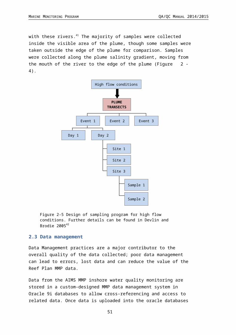
MARINE MONITORING PROGRAM QA/QC MANUAL 2014/2015
The site must be representative of an inshore reef location (as outlined by the initial tender document).
The site is co-located in proximity to sites used by other MMP monitoring activities such as seagrass monitoring, as well as other agencies conducting related monitoring (such as end-of-catchment loads).
The site should not be impacted by specific local point sources such as anti-foulants from boats or inlets of treated or untreated wastewater.
The sampling site can be maintained for a long period.
In addition to the scientific requirements of the project, the selection of passive sampling deployment sites is governed by practicalities which include safety, security, site access, and the availability of a responsible community representative to take responsibility for the maintenance of the site. Site establishment has been a collaborative effort between the agency, AIMS, JCU, and Entox.
The participation of volunteers from various community groups, agencies and tourist operations is a key feature of the routine pesticide monitoring program and integral to the success of maintaining the program in often remote locations. These volunteers assist by receiving, deploying, retrieving and returning the passive samplers to Entox for subsequent extraction and analysis. This active participation of volunteers within the program is made possible by training from the agency and/or Entox staff in Standard Operating Procedures to ensure a high level of continuous sampling and high quality usable data is obtained from these deployments. The agency has taken a lead role in ensuring community involvement and establishing contact with tourism operators and community and regional managers of water quality.
4.2.2 Sampling design - Passive sampling for flood monitoring
In previous monitoring years, pesticides and herbicides were typically monitored during the wet season between November and April using both 1 L grab samples and passive sampling (EDs). These different techniques provide both ‘point in time’ estimates of concentrations, along with time-integrated concentration estimates (using passive samplers deployed over periods of 3 – 14 days). Spatial variation of PSII herbicides in flood plumes is examined by deploying the passive samplers at sites in transects extending from river mouths. Grab samples are also taken along these transects during discharge events when passive samplers are deployed, and also in the pre and post wet season. For this monitoring year (and in the future program), due to budget constraints the passive monitoring component of the flood monitoring was dropped and a more intensive grab sampling campaign will be conducted in two to three focus regions identified as high risk of pesticide exposure. The information collected from the grab sampling will also be used to validate risk models which can inform management about the areas that may be most at risk to acute and chronic exposure to pollutants resulting from river discharge.
51

MARINE MONITORING PROGRAM QA/QC MANUAL 2014/2015
4.2.3 Target Pesticides in the different passive samplers
The chemicals targeted for analysis in the different passive samplers and the limits of reporting (LOR) are indicated in Table 4-6. This list of target chemicals was derived through consultation with GBRMPA with the criteria being:
Detected in recent studies. Recognised as a potential risk (through known usage patterns, amounts and
existing toxicity data). Analytical affordability. Within the current analytical capabilities of Entox or Queensland Health
Forensic and Scientific Services (QHFSS). Likelihood of accumulation in one of the passive samplers (exist as neutral
species in the environment).
Prior to the 2013-14 monitoring year, ED sampler extracts were analysed by Queensland Health using liquid chromatography mass spectrometry (LC-MS) run in positive analysis mode. From the beginning of the 2013 monitoring year, analysis of these extracts was transferred to Entox using an AB Sciex QTRAP 5500 mass spectrometer (AB Sciex, Concord, Ontario, Canada) equipped with an electrospray (TurboV) interface coupled to a Shimadzu Nexera HPLC system (Shimadzu Corp., Kyoto, Japan), also run in positive mode. That year, nine extracts were analysed by both laboratories as an inter-laboratory comparison to validate the Entox analysis. Mean %CV of PSII herbicides detected in a random selection of samples by both laboratories fell within a very acceptable range of 1.9% - 36% (see Table 4-6 in previous years QA/QC report). A small number of extracts will be analysed by both Entox and Queensland Health as an ongoing inter-laboratory validation of Entox methods.
From the 2014-2015 monitoring year onwards, the analysis of ED extracts at Entox will be transferred to a newly acquired LCMS, the AB Sciex QTRAP 6500 (a new model of the QTRAP 5500). The added advantage of this machine is enhanced sensitivity of some analytes, and the ability to analyse in both positive and negative mode in one injection (effectively halving the analysis time required). A comparison of the methods for a small number of samples will be completed, and the results included in the following annual and QA/QC reports. LORs of the target analytes will not be negatively impacted by the change in instrumentation.
PDMS sampler extracts are analysed for pesticides using gas chromatography mass spectrometry (GCMS) by Queensland Health. Entox is currently developing pesticide GCMS methods with a view to completing all analysis ‘in house’ for the 2014-2015 monitoring year.
Prior to the 2013-14 monitoring year, SPE extraction and analysis of PSII herbicides in grab samples was also carried out by Queensland Health. Entox has developed a very sensitive online SPE method that avoids the need for a costly and time consuming traditional SPE extraction and concentration of the sample. LORs are approximately 2 ng/L which exceed those of Queensland Health (10 ng/L). Analysis
52

MARINE MONITORING PROGRAM QA/QC MANUAL 2014/2015
of grab samples for PSII herbicides has now been transferred to Entox. An inter-laboratory comparison between the two methods has not yet been performed. Frozen aliquots of the water samples have been archived to do this comparison retrospectively.
As part of the review process and in consultation with the Pesticide Working Group, the list of target pesticides and herbicides for analysis has been modified to reflect recent changes in pesticide usage, those registered for use in Reef catchments and those frequently detected in passive samplers or water samples by the MMP or other agencies conducting monitoring in the Reef catchments (DSITIA). Table 4-7 lists the proposed priority pesticides to be reported on from 2014 onwards with new inclusions in italics. Analytes where analytical method development is ongoing are noted. Note that this new list includes several priority pesticides and herbicides which may not accumulate well in passive samplers due to their polarity, and may be detectable in grab samples only.
Table 4-7 Pesticides specified under the MMP for analysis in different passive sampler extracts and water samples and the Limits of Reporting (LOR) for these analytesPesticide Description Theoretical LOR - ng/ L
(ED/PDMS), ng/L (water)PDMS^ ED Grab
2,4-D Phenoxy acid herbicide <0.04 – 2 <102,4-DB Phenoxy acid herbicide In developmentAmetryn methylthiotriazine <10 <0.04 – 2 <10Asulam Carbamate herbicide <10Atrazine PSII herbicide-
chlorotriazine<10 <0.04 - 2 <10
Desethylatrazine PSII herbicide breakdown product (also active)
<0.04 - 2 <10
Desisopropylatrazine PSII herbicide breakdown product (also active)
<25 <0.08 - 2 <10
Bromacil PSII herbicide-uracil <0.04 - 2 <10Chlorpyrifos Organophosphate
insecticide<0.5 <10
Diuron PSII herbicide - pheynylurea
<25 <0.04 - 2 <10
Fluazifop Aryloxyphenoxypropionate In developmentFluometuron PSII herbicide-phenylurea <0.08 - 2 <10Fluroxypyr Pyridine carboxylic acid In developmentGlyphosate Glycine In developmentHaloxyfop Aryloxyphenoxypropionate <0.04 - 4 <10Hexazinone PSII herbicide- triazinone <25 <0.04 - 2 <10Imazapic Imidazolinone <0.04 - 2 <10Imidaclorprid Nicotinoid insecticide <0.04 - 4 <10Isoxaflutole Isoxazole In developmentMCPA Phenoxy-carboxylic-acid <0.04 – 2 <10
53

MARINE MONITORING PROGRAM QA/QC MANUAL 2014/2015
Metolachlor Chloracetanilide herbicide <10 <0.04 – 2 <10Metribuzin Triazinone <10 <0.04 – 2 <10Metsulfuron methyl Sulfonylurea herbicide <10 <0.04 – 2 <10MSMA Organoarsenical In developmentParaquat Bipyridylium In developmentPendimethalin Dinitroaniline herbicide In developmentPrometryn PSII herbicide-
methylthiotriazine<5 <0.04 - 2 <10
Propazine PSII herbicide-chlorotriazine
<10
Propiconazole Conazole fungicide <2Simazine PSII herbicide-
chlorotriazine<30 <0.04 - 2 <10
Tebuconazole Conazole fungicide <5Tebuthiruron PSII herbicide-
thiadazolurea<25 <0.04 - 2 <10
Terbutryn PSII herbicides-methylthiotriazine
<0.04 – 0.4
<10
Trifluralin Dintiroaniline <0.5
^If analysed at QHFSS: Grey shading indicates that due to physic-chemical properties, this is unlikely to be a suitable method of sampling; Italics indicate new priority chemicals added to the program
The limits of reporting (LOR) for the LCMS and GCMS instrument data have been defined by Queensland Health Forensic and Scientific Services laboratory as follows: The LORs are determined by adding a very low level amount of analyte to a matrix and injecting 6-7 times into the analytical instrument. The standard deviation of the resultant signals is obtained and a multiplication factor of 10 is applied to obtain the LOR. A further criterion for the LOR is that the analyte value should exceed 3 times the mass detected in the blank. Actual LOR for a given deployment may vary from those indicated in Table 4-7 with any confirmed result converted to a concentration in water estimate and reported.
4.2.4 Passive Sampling Techniques
SDB-RPS Empore discs
3MTM EmporeTM Extraction Disks (SDB-RPS) –Phenomenex.
Deployed in a Teflon “Chemcatcher” housing55 (Figure 4-8).
Routine time integrated monitoring: Deployed with a diffusion limiting 47 mm, 0.45 µm polyether sulfone
membrane for either one month or two months. From January 2012 onwards, Phenomenex membranes of the same specifications were used.
54
MARINE MONITORING PROGRAM QA/QC MANUAL 2014/2015
Deployed in a two disk configuration to extend the time integrated monitoring period when deployed for two months.
Preparation: Condition in methanol for no more than 5 minutes (HPLC grade,
Merck). Condition in milliQ water (Membranes were conditioned in milliQ
water) for a minimum of 5 minutes. Load into acetone rinsed Chemcatcher housing. Cover with membrane and solvent rinsed wire mesh. Fill housing with MilliQ water. Seal for transport. Store in fridge and transport with ice packs.
Extraction: Remove membrane and wipe surface of disk with kimwipe to
remove excess water. Spike disk with labelled internal standard. Extract disk using acetone and methanol in a solvent rinsed 15 mL
centrifuge tube in an ultrasonic bath. Filter (0.22 µm PFTE) and concentrate to 0.5 mL using evaporation
under purified N2. Add ultra-pure water to a final volume of 1 ml. Spike sample with labelled recovery standard
Analyse using LCMS (Table 4-7). Convert to concentration in water using compound specific in situ
sampling rates.
Figure 4-8 An Empore disk (ED) being loaded into the Teflon Chemcatcher housing (LHS) and an assembled housing ready for deployment (RHS)
In-situ calibration of chemicals accumulated in Empore Disks
Compound specific sampling rates have been determined for a broad suite of herbicides and are applied to the estimation of concentrations in water. Sampling rates are influenced by in situ environmental conditions such as flow. A passive flow monitor (PFM), comprised of dental plaster cast into a plastic holder (Figure 4-9), has been developed during the PhD of Dominique O’Brien at Entox as a means
55

MARINE MONITORING PROGRAM QA/QC MANUAL 2014/2015
of flow-adjusting sampling rates using an in situ calibration device.56 The elimination rate of dental plaster from the PFM during the deployment is proportional to flow velocity, and the influence of ionic strength (salinity) on this process has been quantified.57 The sampling rates of reference chemicals in the ED, such as atrazine have subsequently been cross-calibrated to the loss of plaster from the PFM under varying flow conditions (Figure 4-10).58
Figure 4-9 Passive flow monitors (PFMs) prior to deployment (LHS) and post-deployment (RHS)
Figure 4-10 The relationship between flow and the sampling rates of specific herbicides indicating a shift from aqueous boundary layer control to diffusion limiting membrane control under higher flow conditions
The in situ calibration procedure of Empore disks employed at Entox is:
PFMs are co-deployed alongside EDs. Deployment in:
o Wet season (one month).
56

MARINE MONITORING PROGRAM QA/QC MANUAL 2014/2015
o Dry season (two months) – with a flow-limiting cap (reduce loss rate by 15%).
The loss rate of plaster is determined while accounting for the influence of ionic strength.
The sampling rates of atrazine and prometryn are directly predicted from the PFM loss rate using models.
The sampling rates of other individual herbicides are predicted based on the average ratio of the Rs of atrazine to the individual herbicide RS across multiple calibration studies.21,57,59,60 For newly included target herbicides where there is no calibration data available, Entox may adopt the sampling rate of atrazine (and report this consistently throughout the monitoring program to allow inter site and inter-year comparisons) or present the data as ng accumulated per sampler per day.
Presentation and assessment of photosystem II herbicide concentrations (mixtures)
Photosystem II herbicides sampled by the SDB-RPS ED are a priority focus of the MMP pesticide monitoring due to the requirements of the Reef Water Quality Protection Plan.61 The concentrations of individual Photosystem II herbicides (ametryn, atrazine, diuron, hexazinone, flumeturon, prometryn, simazine and tebuthiuron) and atrazine transformation products (desethyl- and desiso-propyl – atrazine) are also expressed as a photosystem II herbicide equivalent concentration (PSII-HEq Equation 3) and assessed against a PSII-HEq Index described previously54 for reporting purposes. PSII-HEq provides a quantitative assessment of PSII herbicide mixture toxicity and assumes that these herbicides act additively.62
From the 2014-2015 monitoring year onwards, we will transition from using the HEq method of risk categorisation to the multi-substances – Potentially Affected Fraction (ms-PAF) method, which will include implementing new risk classes. A comparison between the two methods will be presented in the following annual report.
Polydimethylsiloxane (PDMS) samplers
Silicone rubber 92 cm x 2.5 cm x 410 µm strips. Deployed in a marine grade stainless steel deployment cage (Figure 4-
11). Routine time-integrated (and equilibrium) monitoring:
57
Equation 3PSII−HEq=∑C iREP iWhere:
C i (ng.L-1) is the concentration of the individual PSII herbicide in waterREPi (Dimensionless) is the average relative potency of the individual PSII herbicide with respect to the reference PSII herbicide diuron.

MARINE MONITORING PROGRAM QA/QC MANUAL 2014/2015
o Deployed for approximately one month during the wet season at specific sites only (Table 4-6) and for 2 months in the dry season at one site only.
Preparation:o Dialysis with acetone (2 x 24 hours) and then hexane (2 x 24 hours)
in solvent rinsed glass jars in batches on a shaker.o Strips are loaded with performance reference compounds (PRCs)
see following section.o Stored in solvent rinsed glass jars, with Teflon-lined lids, under
purified N2.o Individual strips are wound around stainless steel spikes within the
deployment cage (acetone rinsed) in a standard configuration.o The cage is assembled and sealed inside a metal can, stored at 4oC
and transported with ice packs. Extraction & purification:
o Biofouling is removed from each strip by scrubbing with water.o Each strip is then dried with kimwipes and spiked with a surrogate
standard.o Each strip is dialysed with 200 mL of hexane (2 x 24 hours).o Sample extracts are rotary evaporated, further evaporated under
purified N2, dried using Na2SO4 columns and filtered (0.45 µm PTFE).
o Samples are made up to 10 ml using dichloromethane and subjected to gel permeation chromatography (GPC).
o The collected fraction is evaporated to 1 ml and submitted for chemical analysis.
Chemical analysis – GCMS.
Figure 4-11 PDMS passive samplers loaded onto stainless steel sampler supports which sits within the deployment cage and is sealed in place with wing nuts
Uploading performance reference compounds (PRCs) into PDMS and the in situ calibration of PDMS
58

MARINE MONITORING PROGRAM QA/QC MANUAL 2014/2015
The dissipation of performance reference compounds (PRCs) to estimate sampling rates of chemicals accumulated in non-polar samplers is an in situ calibration technique that has been extensively discussed.63,64,65 A method based on the work of Booji64 to uniformly upload PRCs into PDMS strips is routinely used at Entox. Whilst the PRC method of adjusting sampling rates is not routinely used (see previous QA/QC report), Entox continues to upload PRCs into samplers.
Alternative method of in situ calibration of PDMS (and SPMDs) using PFMs
O’Brien et al56,58 have previously demonstrated the usefulness of the PFM for the in situ calibration of herbicides in the ED. Furthermore, O’Brien et al66 has demonstrated that the loss of plaster from the PFM can be applied to predict changes in Rs dependant on flow and turbulence, when deploying PDMS or SPMD samplers.
The uptake of bifenthrin, dieldrin, oxadiazon, pendimethalin, permethrin, prothiophos and trifluralin were investigated as a function of water velocity (determined from rPFM) at flows between 0 and 24cm s-1 (Figure 4-12). A one phase association describing this relationship between Rs and flow for each chemical is below (Equation 7).
59
Equation 7Rs= Rs(0 cm/s) + (Rs(max)- Rs(0 cm/s))*(1-exp(-KrPFM *rPFM))
Where:
Rs(0 cm/s) is the Rs of the chemical of interest when exposed to still waters.Rs(max) is the maximum Rs for the chemical of interest KrPFM is a rate constant expressed in reciprocal of the units of rPFM
rPFM is the loss rate of the PFM in g/day.

MARINE MONITORING PROGRAM QA/QC MANUAL 2014/2015
Figure 4-12 PDMS and SPMD sampling rates (Rs) as a function of water velocity rPFM
The in situ calibration procedure of PDMS using PFMs employed at Entox is:
PFMs are co-deployed alongside marine cages containing PDMS. Deployment in:
o Wet season (one month) – without caps.o Dry season (two months) – with a flow limiting cap (reduces plaster
loss rate by 15 %). The loss rate of plaster is determined while accounting for the influence
of ionic strength. Chemical analysis (GCMS) of samplers. Rs of ‘reference’ chemicals - bifenthrin, dieldin, oxadizon, pendimethalin
and permethrin (prothiophos and trifluralin were excluded) - are calculated for each site at their specifc rPFM using Equation 7.
Log Kow of the 7 reference chemicals are plotted against their Rs.
Rs of accumulated chemicals predicted using relationship between Log Kow and Rs of 7 reference chemicals.
Using Rs, estimate Cw using Equation 1. For accumulated chemicals with Log Kow < 4.
i. Equilibrium phase sampling is assumed.ii. Measured Log Ksw (from unpublished collaborative experiment
with DERM, 2010) will be used to estimate a Cw using Equation 2.
60

MARINE MONITORING PROGRAM QA/QC MANUAL 2014/2015
iii. If no measured log Ksw value is available, the Log Ksw will be predicted from the relationship between Log Kow and Log Ksw and the Cw estimated using Equation 2.
For accumulated chemicals with Log Kow > 4, unless otherwise specified, PFM-adjusted Rs will be used to estimate Cw.
The PFM method to predict Rs of chemicals accumulated by PDMS samplers is now routinely used.
Deployment of passive samplers in the field
Figure 4-13 A schematic for the deployment of passive samplers (Empore disc in Chemcatcher housings, and SPMD/PDMS cages) together with the passive flow monitors for in-situ calibration of flow effects, in the field.
4.2.5 QA/QC procedures in the pesticide monitoring program
The development, calibration, field application and validation of passive sampling for monitoring water has been a research focus of Entox over many years. RW.ERROR - Unable to find reference:21347 The methods described above have been developed as a result of this work in collaboration with analytical method development by QHFSS. These methods are formalized as Standard Operating Procedures (SOPs) which describe the preparation, extraction and analysis of each type of passive sampler used in the MMP.
QA/QC procedures routinely employed by Entox in the MMP include:
SOPs for the preparation, deployment, extraction and analysis of passive samplers.
Staff training in these SOPs (laboratory) and a record of this training is maintained.
Deployment guides for the training of field staff & volunteers.
61

MARINE MONITORING PROGRAM QA/QC MANUAL 2014/2015
Generation of a unique alphanumeric identifier code for each passive sampler.
Preparation, extraction, storage (4oC or -20oC) and subsequent analysis of procedural blank passive samplers with each batch of exposed passive samplers.
The use of labelled internal standards or other surrogate standards to evaluate or correct for recovery or instrument sensitivity throughout the extraction and within the analysis process respectively.
The exposure of replicate samplers during each deployment which are extracted and archived in our specimen bank at -80oC.
A proportion of exposed replicate sample extracts are subsequently analysed, to determine the reproducibility of the sampling of organic chemicals across the program in that year (mean normalized difference).
QHFSS laboratories are accredited by the National Association of Standards Testing. Details of QHFSS accreditation can be found at the National Association of Testing Authorities (NATA) website http://www.nata.asn.au/). Sample receipting, handling, analysis and data reporting at QHFSS will be based on NATA certified methods. The NATA accreditation held by the QHFSS includes a wide variety of QA/QC procedures covering the registration and identification of samples with specific codes and the regular calibration of all quantitative laboratory equipment required for the analysis.
4.3 Data Management & Security
The data management protocols for Entox are outlined below and include documentation of all steps within the sampling program: passive sampler identification, transport, deployment, transfer of samples to QHFSS for chemical analysis, analytical results, data manipulation, storage and access. This protocol may be summarized as:
The unique alphanumeric identifier code attached to each passive sampler is applied to all subsequent daughter samples and results, ensuring a reliable link with the original sample.
Deployment Records are sent with the sampling devices, and includes information on: the unique sampling device identifier, deployment identifier, name of the staff/volunteer who performed the operation, storage location, destination site, important dates, details of sample treatment and any problems that may have occurred. When returned, the information is entered into Excel spreadsheets and stored on the Entox main server with a back-up on one local hard drive.
Detailed Chain of Custody records are kept with the samplers at all times. Devices are couriered directly to the tourism operators/community member and monitored via a tracking system. Delivery records are maintained by Entox to ensure traceability of samples.
62

MARINE MONITORING PROGRAM QA/QC MANUAL 2014/2015
Hard copy records maintained of all sample submission forms provided to QHFSS for analysis.
Results files provided by QHFSS along with a unique identifier code are transferred from the instrumentation computer to the Entox server and archived on the QHFSS network using an established data management system.
Excel spreadsheets used for data manipulation and a summary results file (concentration in water estimates) are stored on the Entox server. Access to the Entox server is restricted to authorised personnel only via a password protection system. Provision of data to a third party only occurs at the consent or request of the Program Manager.
4.4 Summary
Unique sample identifiers. Comprehensive Records and Chain of Custody paperwork across all
components. Training of field personnel, including deployment guidelines & records. Analytical Quality Control measures. Procedural QA/QC for the preparation, extraction and analysis of
passive samplers including SOPs. Inclusion of QA/QC samples (replication of sampling and procedural
blanks) Continual evaluation, method development and improvement of
methods for sampler processing & estimation of concentration in water.
63
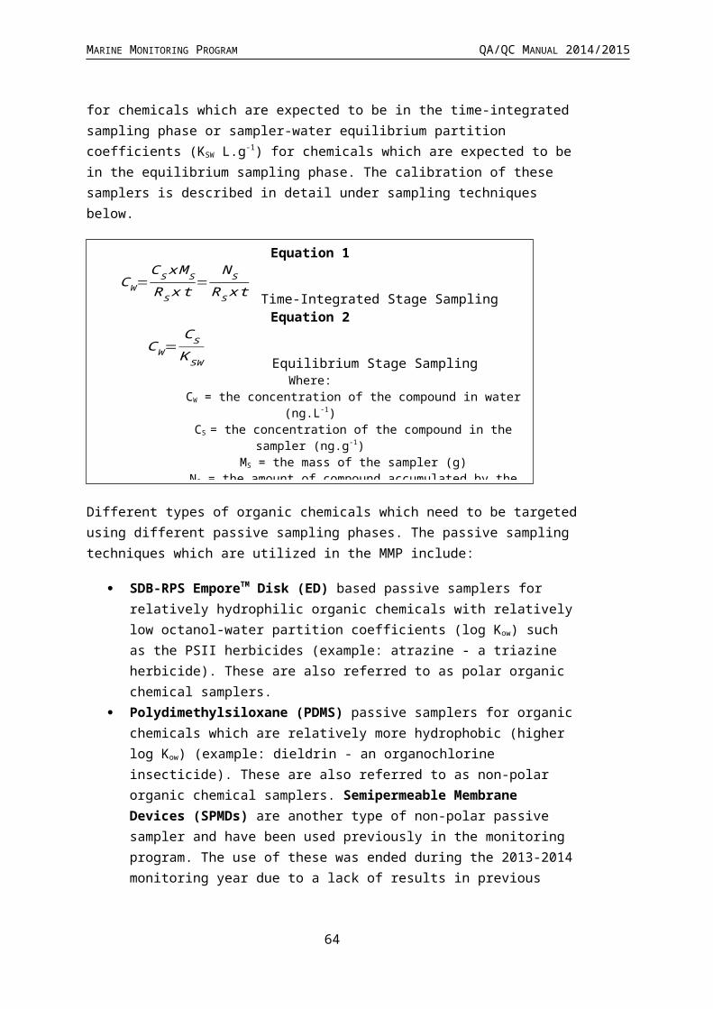
MARINE MONITORING PROGRAM QA/QC MANUAL 2014/2015
5 Inshore coral reef monitoring
Angus Thompson, Johnston Davidson, Paul Costello
Australian Institute of Marine Science
5.1 Introduction
The objective of the biological monitoring of inshore reefs is to document spatial and temporal trends in the benthic reef communities on selected inshore reefs. Changes in these communities may be due to acute disturbances such as cyclonic winds, bleaching and crown-of-thorns starfish as well as more chronic disturbances such as those related to runoff (e.g. increased sedimentation and nutrient loads), which disrupt processes of recovery such as recruitment and growth. A subset of reef monitoring sites are co-located with the sampling locations for lagoon water quality, enabling the assessment of relationship between reef communities and water quality as well as other, more acute impacts.
One salient attribute of a healthy ecological community is that it should be self-perpetuating and ‘resilient’, that is: able to recover from disturbance. One of the ways in which water quality is most likely to shape reef communities is through effects on coral reproduction and recruitment. Laboratory and field studies show that elevated concentrations of nutrients and other agrichemicals and levels of suspended sediment and turbidity can affect one or more of gametogenesis, fertilisation, planulation, egg size, and embryonic development in some coral species (reviewed by Fabricius 20059). High levels of sedimentation can affect larval settlement or net recruitment of corals. Similar levels of these factors may have sub-lethal effects on established adult colonies. Because adult corals can tolerate poorer water quality than recruits and colonies are potentially long-lived, reefs may retain high coral cover even under conditions of declining water quality, but have low resilience. Some high-cover coral communities may be relic communities formed by adult colonies that became established under more favourable conditions. Such relic communities would persist until a major disturbance, but subsequent recovery may be slow if recruitment is reduced or non-existent. This would lead to long term degradation of reefs, since extended recovery time increases the likelihood that further disturbances will occur before recovery is complete.76 For this reason, the surveys for the MMP estimate cover of various coral taxa and also collect information on the abundance of juvenile colonies as evidence for the extent of ongoing recruitment.
This component of the MMP aims to accurately quantify temporal and spatial variation in inshore coral reef community status in relation to variations in local reef water quality. A detailed report77 linked the consistent spatial patterns in coral community composition observed over the first three years of the project with environmental parameters. As the temporal span of this project extends, there has been a natural shift in the focus toward understanding and documenting the
64

MARINE MONITORING PROGRAM QA/QC MANUAL 2014/2015
differences in community dynamics (status) across the spatial extent of the sampling rather than reiterating spatial differences in composition.
In order to quantify inshore coral reef community status in relation to variations in local reef water quality, this project has several key objectives:
Provide an annual time series of benthic community structure (viz. cover and composition of sessile benthos such as hard corals, soft corals and algae) for inshore reefs as a basis for detecting changes related to water quality and disturbances.
Provide information about coral recruitment on Reef inshore reefs as a measure for reef resilience.
Provide information about sea temperature as a potential driver of environmental conditions at inshore reefs.
Provide an integrated assessment of coral community condition for the inshore reefs monitored to serve as a report card against which changes in condition can be tracked.
5.2 Methods
5.2.1 Sampling design
The sampling design was selected for the detection of change in benthic communities on inshore reefs in response to improvements in water quality parameters associated to specific catchments, or groups of catchments (Region), and to disturbance events. Within each Region, reefs are selected along a gradient in exposure to run-off, largely determined as increasing distance from a river mouth in a northerly direction. To account for spatial heterogeneity of benthic communities within reefs, two sites were selected at each reef (Figure 5-14).
65

MARINE MONITORING PROGRAM QA/QC MANUAL 2014/2015
Figure 5-14 Sampling design for coral reef benthic community monitoring. Terms within brackets are nested within the term appearing
Observations on a number of inshore reefs undertaken by AIMS in 2004 during the pilot study to the current monitoring program78 highlighted marked differences in community structure and exposure to perturbations with depth; hence sampling within sites is stratified by depth. Within each site and depth, fine scale spatial variability is accounted for by the use of five replicate transects.
5.2.2 Site selection
The reefs monitored were selected by the agency, using advice from expert working groups. The selection of reefs was based upon two primary considerations:
To ensure sampling locations in each catchment of interest were spread along a perceived gradient of influence from river output.
Those sites are selected where there was evidence (in the form of carbonate-based substrate) that coral reef communities had been viable (net positive accretion of a carbonate substrate) in the past.
Where well-developed reefs existed on more than one aspect of an island, two reefs are included in the design as although position relative to runoff exposure is similar, often quite different communities exist on windward compared to leeward reefs.
Over time there have been some adjustments to the sampling design (Table 5-8). For the first two years of the project (2005 and 2006) 35 reefs were surveyed each year. In 2007 to 2014 the fringing reefs along the Cape Tribulation coast were no longer surveyed due to concerns over crocodile attack. In addition the sampling frequency changed so that only a subset of “core” reefs were surveyed every year with the remaining “cycle” reefs surveyed every other year (Table 5-8). From 2015 the sampling changed again with King Reef replaced by Bedarra Island in the Tully
66

MARINE MONITORING PROGRAM QA/QC MANUAL 2014/2015
Catchment and all reefs changed to sampling frequency of once every two years (Table 5-8). A map of sites included from 2015 is presented as Figure 5-15.
5.2.3 Depth selection
From observations of a number of inshore reefs undertaken by AIMS in 200478, marked differences in community structure and exposure to perturbations with depth were noted. The lower limit for the inshore coral surveys was selected at 5m below datum, because coral communities rapidly diminish below this depth at many reefs; 2m below datum was selected as the shallow depth as this allowed surveys of the reef crest. Shallower depths were considered but discounted for logistical reasons, including the inability to use the photo technique in very shallow water, site markers creating a danger to navigation and difficulty in locating a depth contour on very shallow sloping substrata typical of reef flats.
5.2.4 Field survey methods
Site marking
Each selected reef sites are permanently marked with steel fence posts at the beginning of each twenty-metre transect and smaller (10 mm diameter) steel rods at the ten metre mark and end of each transect. Compass bearings coupled with distance along transects record the transect path between these permanent markers. Transects were set initially by running two sixty-metre fibreglass tape measures out along the desired five or two metre depth contour. Digital depth gauges are used along with tide heights from the closest location included in ‘Seafarer Tides’ electronic tide charts produced by the Australian Hydrographic Service. There are five-metre gaps between each consecutive 20 metre transect. The position of the first picket of each site is recorded by GPS.
Sampling methods
Three separate sampling methodologies are used to describe the benthic communities of inshore coral reefs. These are each conducted along the fixed transects identified in the sampling design though there are subtle differences in width or length of transect or spatial extent of the data sets as listed in Table 5-8.
Photo Point Intercept Method (PPIT)
This method is used to gain estimates of the per cent cover of benthic community components. The method follows closely the Standard Operational Procedure Number 10 of the AIMS Long Term Monitoring Program.79 In short, digital photographs are taken at 50-centimetre intervals along each 20-metre transect. Estimation of cover of benthic community components is derived from the identification of the benthos lying beneath points overlaid onto these images. For the majority of hard and soft corals at least genus level identification is achieved. The categories used for identification of benthos are listed in Jonker, M. et al 2008. 79
67

MARINE MONITORING PROGRAM QA/QC MANUAL 2014/2015
The primary difference in the application of the method in this project from that described in Jonker et al. 200879 is in the sampling design. Sampling for this project is based on 20-metre transects, rather than 50-metre transects. To compensate for transects being shorter than in the standard method, the density of frames per unit area of transect is doubled (images captured at 0.5 m rather than one-metre intervals). This alteration to the standard technique was adopted due to the limited size of some reefs sampled.
Figure 5-15 Coral community sampling locations as at 2015
68

MARINE MONITORING PROGRAM QA/QC MANUAL 2014/2015
Table 5-8 Sites selected for inshore reef monitoring.For sites sampled in 2005-2014 those in bold were core reefs surveyed every year, those in plain font were cycle reefs surveyed every other year, those in italic where not surveyed post 2006, and all reefs were surveyed in 2005 and 2006. From 2015 the sampling frequency reduced to once every two years for all reefs with those in bold sampled in odd numbered years and those in plain font in even numbered years.
NRM Region Catchment 2005-2014 2015 on Team
Wet Tropics
Daintree Cape Tribulation (North)Cape Tribulation (Mid)Cape Tribulation (South)Snapper Island (North)Snapper Island (South)
Snapper Island (North)Snapper Island (South)
Sea Research
Russell / Mulgrave Johnstone
Fitzroy Island (East)Fitzroy Island (West)Frankland Island Group (East)Frankland Island Group (West)High Island (East)High Island (West)
Fitzroy Island (East)Fitzroy Island (West)Frankland Island Group (East)Frankland Island Group (West)High Island (East)High Island (West)
AIMS
Tully Dunk Island (North)Dunk Island (South)North Barnard GroupKing Reef
Dunk Island (North)Dunk Island (South)North Barnard GroupBedara
AIMS
Burdekin
Herbert Lady Elliot ReefOrpheus Island (East)Pelorus Is & Orpheus Is (West)
Lady Elliot ReefOrpheus Island (East)Pelorus Is & Orpheus Is (West)
AIMS
Burdekin Geoffrey BayMiddle ReefPandora ReefHavannah Island
Geoffrey BayPandora ReefHavannah Island
AIMS
69

MARINE MONITORING PROGRAM QA/QC MANUAL 2014/2015
NRM Region Catchment 2005-2014 2015 on Team
Mackay Whitsunday
Proserpine Pine IslandShute IslandDaydream IslandDouble Cone IslandSeaforth IslandDent IslandHook Island
Pine IslandShute IslandDaydream IslandDouble Cone IslandSeaforth IslandDent IslandHook Island
AIMS
Fitzroy
Fitzroy Peak IslandPelican IslandHumpy & Halfway IslandsMiddle IslandNorth Keppel IslandBarren Island
Peak IslandPelican IslandHumpy & Halfway IslandsMiddle IslandNorth Keppel IslandBarren Island
AIMS
Table 5-9 Distribution of sampling effort
Survey Method
Information provided Transect coverage Spatial
coverage
Photo Point Intercept
Percentage cover of the substrate of major benthic habitat components.
Approximately 25 cm belt along upslope side of transect form which 160 points are sampled.
Full sampling design
Demography
Size structure of coral communities, density post settlement recruitment
34 cm belt along the upslope side of the transect.
Full sampling design
Scuba Search
Incidence of factors causing coral mortality
Two-metre belt centred on transect
Full sampling design
Juvenile coral surveys
This survey aims to provide an estimate of the number of coral colonies that were successfully recruiting to and surviving early post-settlement pressures. In the first
70

MARINE MONITORING PROGRAM QA/QC MANUAL 2014/2015
year of sampling under this program these juvenile coral colonies were counted as part of a demographic survey that counted the number of individuals falling into a broader range of size classes. As the focus narrowed to just juvenile colonies the number of size classes reduced allowing an increase in the spatial coverage of sampling.
Coral colonies less than ten centimetres in diameter are counted within a belt 34 cm wide (data slate length) along the upslope side of each 20-metre transect. Each colony is identified to genus and assigned to a size class of either, 0-2 cm, >2-5 cm, or >5-10 cm. Importantly this method aims at estimating the number of juvenile colonies that result from the settlement and subsequent survival and growth of coral larvae rather than small coral colonies resulting from fragmentation or partial mortality of larger colonies. With the exception of the transect dimension and the size classes used, this method is consistent with the Standard Operational Procedure Number 10 of the AIMS Long-term Monitoring Program79, Part 2, in which further detail relation to juvenile/fragment differentiation can be found.
Scuba Search Transects
Scuba search transects document the incidence of agents causing coral mortality or disease. Tracking of these agents of mortality is important as declines due to these agents must be carefully considered as covariates for possible trends associated with response to outcomes. The method used follows closely the Standard Operational Procedure Number 9 of the AIMS Long Term Monitoring Program80, Part 2. In short, a search is made of a two-metre wide belt (one metre either side of the transect midline) for any recent scars, bleaching, disease or damage to coral colonies. An additional category not included in the standard procedure is physical damage. This is recorded on the same five-point scale as coral bleaching and describes the proportion of the coral community that has been physically damaged, as indicated by toppled or broken colonies. This category may include anchor as well as storm damage.
5.2.5 Observer training
The AIMS personnel collecting data in association with this project are without exception highly experienced in the collection of benthic monitoring data. Each observer was employed specifically for their skills in benthic monitoring and video analysis.
Ongoing standardisation of observers is achieved through in field and photo based comparisons that for the most mitigate inconsistencies in identification. As a final step in reducing bias in sampling all photo transect identifications are double checked by a single observer.
In the event that new observers enter the team, training in each sampling method is by direct tuition with an experienced observer. New observers must meet the standards listed in Table 5-10 prior to collecting data for the project.
71

MARINE MONITORING PROGRAM QA/QC MANUAL 2014/2015
Classification to genus level underwater is augmented by the use of a small digital camera to take images for post-dive scrutiny of difficult to identify colonies. We do note however that some small juvenile corals are difficult to differentiate in the field and while identified to genus level are typically merged with similar genera for analysis and reporting.
Sea Research is responsible for surveys in the Daintree catchment. The Sea Research observer, Tony Ayling, is the most experienced individual in Australia in surveying the benthic communities of near-shore coral reefs. He has 30-years experience surveying the sites in this catchment, amongst many others. His taxonomic skills are undoubted at genus level and as such observer standardisation for demography and scuba search surveys are limited to detailed discussion of methodologies with AIMS observers and explicit following of the protocols listed here. Sea Research will also use the same pre-printed datasheets and data entry programs. Analysis of video footage collected by Sea Research will be undertaken by AIMS.
Table 5-10 Observer training methods and quality measuresMonitoring method Training method Quality measure
Photo Point Intercept
In-field identification of benthic components.On screen classification of photo points.In-field tuition on photographic protocol.
All identifications double checked.
Juvenile counts
In-field identification of corals to genus level, and application of technique with experienced observer supervision.
No greater than ten percent of colonies misidentified, overlooked or misclassified in size during supervised demographic surveys of two sites.
Scuba Search In-field tuition in the
classification of coral scars and damage.
Observation of at least ninety percent of damaged colonies and their correct classification during supervised surveys of two sites of damaged colonies.
5.2.6 Temperature monitoring
Temperature loggers are deployed at, or in close proximity to, all locations at both two-metre and five-metre depths and routinely exchanged at the time of the coral surveys (i.e. every 12 or 24 months). Three types of temperature loggers have been used for the sea surface temperature logger program. The first type was the Odyssey temperature loggers (http://www.odysseydatarecording.com/) these were superseded by the Sensus Ultra Temperature logger (http://reefnet.ca/products/sensus/). In 2015 Vemco minilog temperature loggers (http://vemco.com/products/minilog-ii-t/) began to replace aging Sensus loggers
72
MARINE MONITORING PROGRAM QA/QC MANUAL 2014/2015
The Odyssey loggers were set to take readings every thirty minutes. The Sensus and Vemco loggers were set to take readings every 10 minutes. Loggers were calibrated against a certified reference thermometer after each deployment and generally accurate to ± 0.2°C.
Detailed data download, quality checks and data management methods are described in Appendix A12.
5.3 Data management
Data Management practices are a major contributor to the overall quality of the data collected; poor data management can lead to errors, lost data and can reduce the value of the Reef Plan MMP data. Data from the AIMS MMP inshore coral reef monitoring are stored in a custom-designed MMP data management system in Oracle 9i databases to allow cross-referencing and access to related data. Once data are uploaded into the oracle databases after the quality assurance and validation processes, they are consolidated in an Access Database via oracle views. The Access Database product was chosen as the delivery mechanism for its simplicity and because most users are familiar with the software (see Appendix A12 for details about general AIMS in-house procedures for data security, data quality checking and backup).
It is AIMS policy that all data collected have a metadata record created for it. The metadata record is created using a Metadata Entry System where the metadata is in the form of ISO19139 XML. This is the chosen format for many agencies across Australia and the International Community that deal with spatial scientific data. You can visit AIMS Metadata System at:
http://data.aims.gov.au/geonetwork/srv/en/main.home.
All coral monitoring field data is recorded on pre-printed datasheets. The use of standard data sheets aids in ensuring standard recording of attributes, and ensures required data are collected.
On return from the field, all data is entered on the same day into database forms linked directly to an Oracle Lite database. Each field on these forms mirror those on pre-printed data sheets and include lookup fields to ensure data entered is of appropriate structure or within predetermined limits. For example, entry of genera to the demography data table must match a pre-determined list of coral genera.
On return to the office, the data is uploaded to an Oracle Database using the Oracle Lite synchronization process. All keyed data is printed and checked against field data sheets prior to final logical checking (ensuring all expected fields are included and tally with number of surveys). Photo images are also stored on a server that is included in a routine automatic back up schedule. Photo images are burnt to DVD prior to analysis as a second backup.
73

MARINE MONITORING PROGRAM QA/QC MANUAL 2014/2015
Image analysis of reef monitoring photos is performed within the AIMS monitoring data entry package “reefmon”. This software contains logical checks to all keyed data and is directly linked to a database to ensure data integrity. The directory path to transect images is recorded in the data base. This functionality allows the checking of benthic category identification. All photo transect data is checked by a second experienced observer prior to data analysis and reporting of results.
5.4 Summary of Quality Control measures
Use of published Standard Operational Procedures. Prior to the field data collection staff are trained and assessed by
experienced observers to ensure their identification skills are consistent with the resolution required.
Data entry via database forms that include logical checking on format and content of entered fields, and confirmation of data by second observer.
Continual evaluation, method development and improvement of methods. Advanced data management and security procedures.
74

MARINE MONITORING PROGRAM QA/QC MANUAL 2014/2015
6 Intertidal seagrass monitoring1Len McKenzie, 2Michelle Waycott, 3Richard Unsworth, 1Catherine Collier
1Centre for Tropical Water & Aquatic Ecosystem Research (TropWATER), James Cook University, Cairns, QLD2 University of Adelaide / Plant Biodiversity Centre, Department of Environment and Natural Resources, Adelaide, SA 3Seagrass Ecosystem Research Group, College of Science, Wallace Building, Swansea University SA2 8PP, UK
6.1 Introduction
Approximately 3,063 square kilometres of inshore seagrass meadows has been mapped in Great Barrier Reef World Heritage Area waters shallower than 15 metres, relatively close to the coast, and in locations that can potentially be influenced by adjacent land use practices. Monitoring of the major marine ecosystem types most at risk from land-based sources of pollutants is being conducted to ensure that any change in their status is identified. Seagrass monitoring sites are associated with the river mouth and inshore marine water quality monitoring tasks in the MMP to enable correlation and concurrently collected water quality information.
The key aims of the inshore seagrass monitoring under the MMP are to:
Understand the status and trend of Reef inshore seagrass (detect long-term trends in seagrass abundance, community structure, distribution, reproductive health, and nutrient status from representative inshore seagrass meadows).
Identify response of seagrass to environmental drivers of change. Integrate reporting on Reef seagrass status including production of seagrass
report card metrics for use in an annual Paddock to Reef report card.
6.2 Methods
6.2.1 Sampling design
The sampling design was selected to detect change in inshore seagrass community status to compare with seagrass environmental status (water quality) in relation to specific catchments or groups of catchments (NRM region). Within each region, a relatively homogenous section of a representative seagrass meadow is selected to represent each of the seagrass habitats present (estuarine, coastal, reef) (habitat (Region)). Meadow selection was informed using mapping surveys across the regions prior to site establishment, and by the GBRMPA, using advice from expert working groups. To account for spatial heterogeneity, two sites are selected within each location (Site [Habitat (Region)]). Subtidal sites are not replicated within locations. Within each site, finer scale variability is accounted for by using three 50-metre transects nested in each site. The final constraint on site selection is that the Minimum Detectable Difference (MDD) must be below 20% (at the 5% level of significance with 80% power). A site is defined as a 50mx50m area. The sampling strategy for subtidal sites is modified to sample along 50m transects 2-3 m apart
75
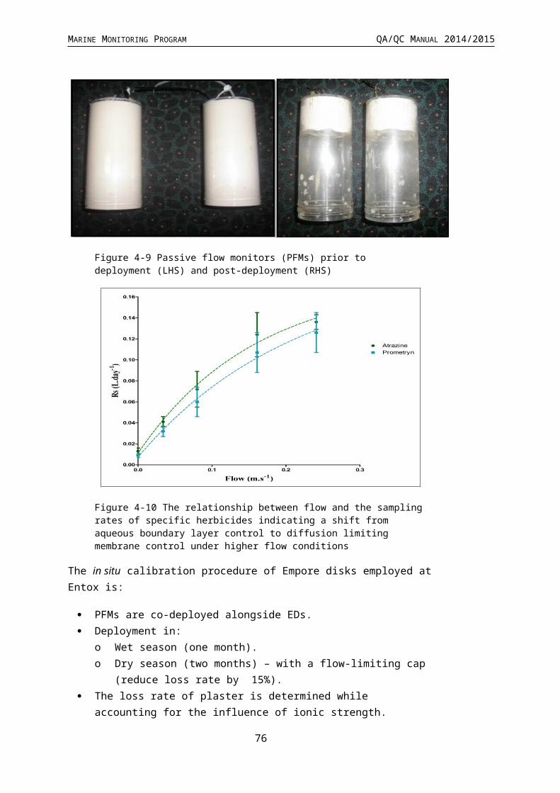
MARINE MONITORING PROGRAM QA/QC MANUAL 2014/2015
(aligned along the depth contour) due to logistical purposes of SCUBA diving in often poor visibility. At each site, monitoring is conducted during the late-monsoon (April) and late-dry (October) periods each year; additional sampling is conducted at more accessible locations in the dry (July) and monsoon (January).
6.2.2 Field survey methods - Inshore seagrass meadow abundance, community structure and reproductive health
Site marking
The sampling locations for this program are listed in Figure 6-16 and Table 6-11. Each selected inshore seagrass site is permanently marked with plastic star pickets at the 0 m and 50 m points of the centre transect. Labels identifying the sites and contact details for the program are attached to these pickets. Positions of 0 m and 50 m points for all three transects at a site are also noted using GPS (accuracy ±3 m). This ensures that the same site is monitored each event.
76

MARINE MONITORING PROGRAM QA/QC MANUAL 2014/2015
Figure 6-16 Inshore seagrass monitoring sites for the Marine Monitoring Program
Seagrass cover and species composition
Survey methodology follows standard methodology81 (Appendix D1). A site is defined as an area within a relatively homogenous section of a representative seagrass community/meadow.82
Monitoring at the 45 sites identified for the MMP long-term inshore monitoring in late-monsoon (April) and late-dry season (October) of each year is conducted by qualified and trained scientists who have demonstrated competency in the methods (see 6.2.3). Monitoring conducted outside these periods is also conducted by a trained scientist, and at 3 locations (Magnetic Island, Townsville and Pioneer Bay) is assisted by volunteers.
At each site, during each survey, observers record the percent seagrass cover within a 50 cm × 50 cm quadrat every 5 m along three 50m transects, placed 25m
77

MARINE MONITORING PROGRAM QA/QC MANUAL 2014/2015
apart. A total of 33 quadrats are sampled per site. Seagrass abundance is visually estimated as the fraction of the seabed (substrate) obscured by the seagrass species when submerged and viewed from above. This method is used because the technique has wider application and is very quick, requiring only minutes at each quadrat; yet it is robust and highly repeatable, thereby minimising among-observer differences. Quadrat percent cover measurements have also been found to be far more efficient in detecting differences in seagrass abundance than seagrass blade counts or measures of above- or below-ground biomass. To improve resolution and allow greater differentiation at very low percentage covers (e.g. <3%), shoot counts based on global species density maxima are used. For example: 1 pair of Halophila ovalis leaves in a quadrat = 0.1%; 1 shoot/ramet of Zostera in a quadrat = 0.2%. Additional information is collected at the quadrat level, including: seagrass canopy height of the dominant strap leaved species; macrofaunal abundance; abundance of burrows, as a measure of bioturbation; presence of herbivory (e.g. dugong and sea turtle); a visual/tactile assessment of sediment composition (see McKenzie 2007)83; and observations on the presence of superficial sediment structures such as ripples and sand waves to provide evidence of physical processes in the area (see Koch 2001)84.
Seagrass reproductive health
An assessment of seagrass reproductive health at locations identified in Table 6-11 via flower production and seed bank monitoring is conducted in late-dry season (October) of each year at each site. Additional collections are also conducted in late-monsoon (April) where possible.
In the field, 15 haphazardly placed cores (100mm diameter x 100mm depth) of seagrass are collected from an area adjacent, of similar cover and species composition, to each monitoring site. All samples collected are given a unique sample code/identifier providing a custodial trail from the field sample to the analytical outcome.
Seeds banks and abundance of germinated seeds are sampled according to standard methods 81 by sieving (2mm mesh) 30 cores (50mm diameter, 100mm depth) of sediment collected across each site and counting the seeds retained in each. For Zostera muelleri subsp. capricorni, where the seeds are <1mm diameter, intact cores (18) are collected and returned to the laboratory where they are washed through a 710µm sieve and seeds identified using a hand lens/microscope.
Seagrass tissue nutrients
Collection of seagrass leaf tissue (targeted foundation genus include Halodule, Zostera and Cymodocea) for analysis of tissue nutrients (C, N, P, δ15N, δ13C) is conducted in the late-dry season (October) sampling period at regions identified in Table 6-11. Approximately five to 10 grams wet weight of seagrass leaves is harvested from three to six haphazardly chosen plots (two to three m apart) in an area adjacent, of similar cover and species composition, to each monitoring site. All
78

MARINE MONITORING PROGRAM QA/QC MANUAL 2014/2015
samples collected are given a unique sample code/identifier providing a custodial trail from the field sample to the analytical outcome.
Rhizosphere sediment herbicide (haphazard)
Sediment samples (approximately 250ml) for analysis of herbicide concentrations are collected in late-monsoon (April) at selected monitoring sites when funding is available. Rhizosphere herbicide samples are obtained using a stainless steel spoon and bowl rinsed with acetone between each sample collection. Approximately 20ml of sediment is collected every five metres along each transect to a depth approximately equal to the depth of the rhizome layer. Three homogenised samples (one per each transect) were collected per site. The samples are stored in acetone rinsed Teflon lidded jars provided by the QHFSS. Sediments are kept frozen until analyses by the NATA accredited commercial laboratory at the QHFSS.
6.2.3 Observer training
The JCU personnel collecting data in association with this project are without exception highly experienced in the collection of seagrass monitoring data. The majority of observers have been involved in seagrass monitoring for at least a decade and were employed specifically for their skills associated with the tasks required.
All observers have successfully completed at Level 1 Seagrass-Watch training course (seagrasswatch.org/training.html) and have demonstrated competency across 7 core units: achieved 80% of formal assessment (classroom and laboratory) (5 units); and demonstrated competency in the field both during the workshop (1 unit) and post workshop (1 unit = successful completion of 3 monitoring events/periods within 12 months). Volunteers who assist JCU scientists have also successfully completed a Level 1 training course.
Technical issues concerning quality control of data are important and are resolved by: using standard methods which ensure completeness in the field (the comparison between the amounts of valid or useable data originally planned to collect, versus how much was collected); using standard seagrass cover calibration sheets to ensure precision (the degree of agreement among repeated measurements of the same characteristic at the same place and the same time) and consistency between observers and across sites at monitoring times. Ongoing standardisation of observers is achieved through routine comparisons during sampling events. Any discrepancy is used to identify and subsequently mitigate bias. For the most part however uncertainties in percentage cover or species identification are mitigated in the field via direct communication, or the collection of voucher specimens (to be checked under microscope and pressed in herbarium) and the use of a digital camera to record images (protocol requires at least 27% of quadrats are photographed) for later identification and discussion. Evidence of competency is securely filed on a secure server in Cairns at James Cook University
79
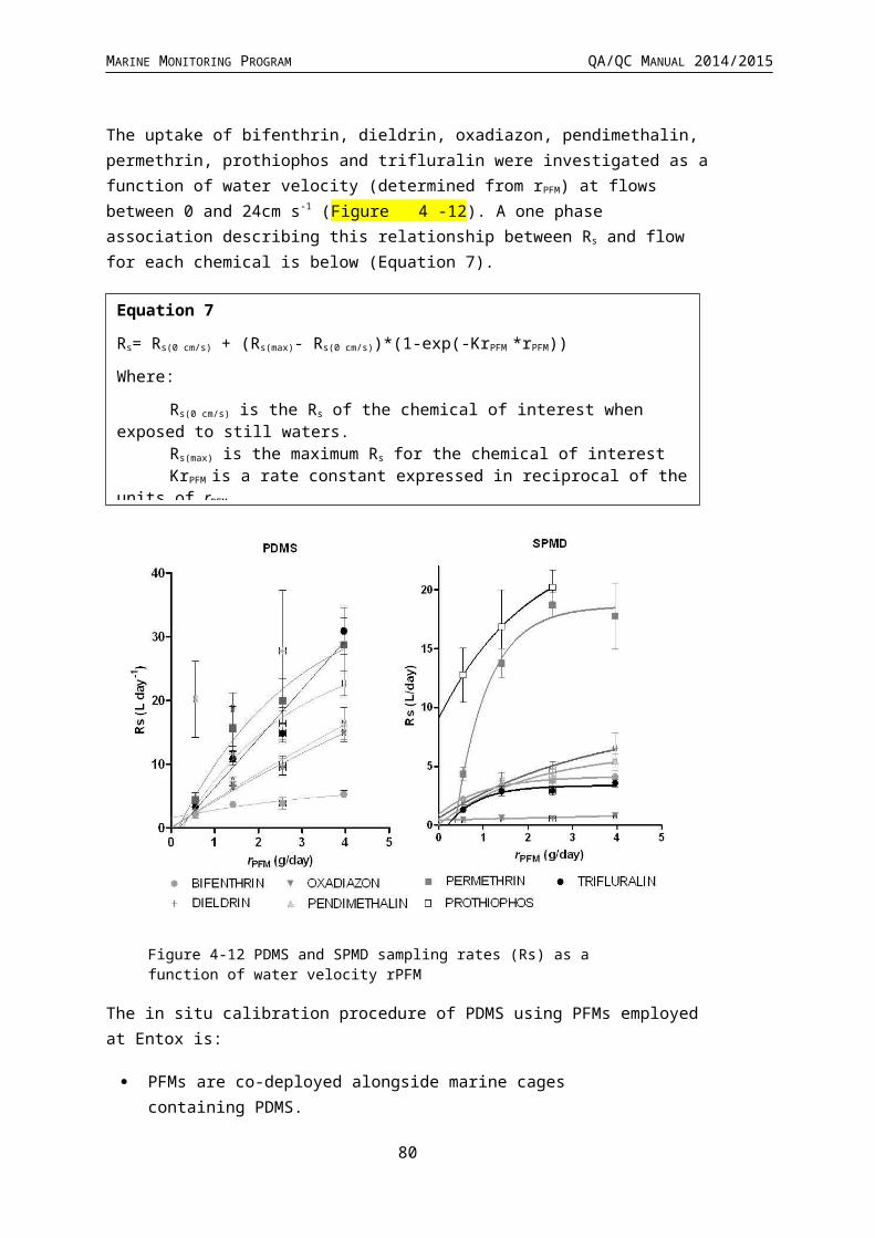
MARINE MONITORING PROGRAM QA/QC MANUAL 2014/2015
Howley Consulting is responsible for surveys in the Cooktown region. The Howley Consulting observer, Christina Howley, has been assessing seagrass resources in the Cape York region for over a decade and has successfully completed a Level 1 training course.
80

MARINE MONITORING PROGRAM QA/QC MANUAL 2014/2015
Table 6-11 MMP inshore seagrass long-term monitoring sites
NRM region from www.nrm.gov.au. * = intertidal, ^=subtidal.
RegionNRM
region (Board)
Catchment Monitoring location Site Latitude Longitude Seagrass community type
Far Norther
n
Cape York
Shelburne Baycoastal
SR1* Shelburne Bay 11°
53.233
142°
54.851 H. ovalis with H. uninervis/T. hemprichii
SR2* Shelburne Bay 11°
53.251
142°
54.938 H. ovalis with H. uninervis/T. hemprichii
Piper Reefreef
FR1* Farmer Is. 12°15.352
143°
14.020 T. hemprichii with C. rotundata/H. ovalis
FR2* Farmer Is. 12°15.448
143°
14.185 T. hemprichii with C. rotundata/H. ovalis
Normanby
Stanley Islandreef
ST1* Stanley Island 14°
8.576
144°
14.680
H. ovalis/H. uninervis with T. hemprichii/C. rotundata
ST2* Stanley Island 14°
8.547
144°
14.588
H. ovalis/H. uninervis with T. hemprichii/C. rotundata
Bathurst Baycoastal
BY1* Bathurst Bay 14°16.082
144°
13.961
H. uninervis with H. ovalis/T. hemprichii/C. rotundata
BY2* Bathurst Bay 14°16.062
144°
13.896
H. uninervis with H. ovalis/T. hemprichii/C. rotundata
Endeavour Cooktownreef
AP1* Archer Point 15° 36.500
145°
19.143
H. univervis/ H. ovalis with Cymodocea/T. hemprichii
AP2* Archer Point 15° 36.525
145°
19.108 H. univervis/H. ovalis with C. rotundata
Northern
Wet Tropics(Terrain NRM)
Mossman Low Islesreef
LI1* Low Isles 16° 23.11
145° 33.88 H.ovalis/H.uninervis
LI2^ Low Isles 16° 22.97
145° 33.85 H.ovalis/H.uninervis
BarronRussell -Mulgrave
Cairnscoastal YP1* Yule Point 16° 34.1
59145°
30.744 H. uninervis with H. ovalis
YP2* Yule Point 16° 33.8 14 30.55 H. uninervis with H. ovalis
81

MARINE MONITORING PROGRAM QA/QC MANUAL 2014/2015
Johnstone
32 5° 5
Green Islandreef
GI1* Green Island 16° 45.789
145° 58.31 C. rotundata/T. hemprichii with H.
uninervis/H. ovalis
GI2* Green Island 16° 45.776
145°
58.501
C. rotundata/T. hemprichii with H. uninervis/H. ovalis
GI3^ Green Island 16° 45.29
145° 58.38 C. rotundata/ H.
uninervis/C.serrulata/S.isoetifolium
Tully
Mission Beachcoastal
LB1* Lugger Bay 17° 57.645
146° 5.61 H. uninervis
LB2* Lugger Bay 17° 57.674
146° 5.612 H. uninervis
Dunk Islandreef
DI1* Dunk Island 17° 56.6496
146°
8.4654
H. uninervis with T. hemprichii/ C. rotundata
DI2* Dunk Island 17° 56.7396
146°
8.4624
H. uninervis with T. hemprichii/ C. rotundata
DI3^ Dunk Island 17° 55.91
146° 08.42 H. uninervis / H. ovalis/H.decipiens/C.
serrulataCentral
Burdekin(NQ Dry Tropics)
Burdekin
Magnetic islandreef
MI1* Picnic Bay 19° 10.734
146°
50.468
H. uninervis with H. ovalis & Zostera/T. hemprichii
MI2* Cockle Bay 19° 10.612
146°
49.737
C. serrulata/ H. uninervis with T. hemprichii/H. ovalis
MI3^ Picnic Bay 19° 10.734
146°
50.468
H. uninervis with H. ovalis & Zostera/T. hemprichii
Townsvillecoastal
SB1* Shelley Beach 19° 11.0
46146°
45.697 H. uninervis with H. ovalis
BB1* Bushland Beach 19° 11.0
28146°
40.951 H. uninervis with H. ovalis
Bowling Green Bay
coastal
JR1* Jerona (Barratta CK)
19° 25.380
147°
14.480 H. uninervis with Zostera/H. ovalis
JR2* Jerona (Barratta CK)
19° 25.281
147°
14.425 H. uninervis with Zostera/H. ovalis
Mackay Whitsund
ay
Proserpine Whitsundayscoastal PI2* Pioneer Bay 20° 16.1
76148°
41.586 H. uninervis/ Zostera with H. ovalis
PI3* Pioneer Bay 20° 16.2 14 41.84 H. uninervis with Zostera/H. ovalis
82

MARINE MONITORING PROGRAM QA/QC MANUAL 2014/2015
(Reef Catchme
nts)
48 8° 4
Whitsundaysreef
HM1* Hamilton Island 20°
20.7396
148°
57.5658 H. uninervis with H. ovalis
HM2* Hamilton Island 20° 20.8
02148°
58.246 Z. muelleri with H. ovalis/H. uninervis
Pioneer Mackayestuarine
SI1* Sarina Inlet 21° 23.76
149° 18.2 Z. muelleri with H. ovalis (H. uninervis)
SI2* Sarina Inlet 21° 23.712
149°
18.276 Z. muelleri with H. ovalis (H. uninervis)
Southern
Fitzroy(Fitzroy Basin
Association)
Fitzroy
Shoalwater Baycoastal
RC1* Ross Creek 22° 22.953
150°
12.685 Zostera muelleri with H. ovalis
WH1* Wheelans Hut 22° 23.9
26150°
16.366 Zostera muelleri with H. ovalis
Keppel Islandsreef
GK1* Great Keppel Is. 23°
11.783
150°
56.3682 H. uninervis with H. ovalis
GK2* Great Keppel Is. 23° 11.6
37150°
56.3778 H. uninervis with H. ovalis
BoyneGladstone Harbourestuarine
GH1* Gladstone Hbr 23° 46.0
05151°
18.052 Zostera muelleri with H. ovalis
GH2* Gladstone Hbr 23° 45.8
74151°
18.224 Zostera muelleri with H. ovalis
Burnett Mary
(Burnett Mary
Regional Group)
Burnett Rodds Bayestuarine
RD1* Rodds Bay 24° 3.4812
151°
39.3288 Zostera muelleri with H. ovalis
RD2* Rodds Bay 24° 4.866
151°
39.7584 Zostera muelleri with H. ovalis
Mary Hervey Bayestuarine
UG1* Urangan 25° 18.053
152°
54.409 Zostera muelleri with H. ovalis
UG2* Urangan 25° 18.197
152°
54.364 Zostera muelleri with H. ovalis
83

MARINE MONITORING PROGRAM QA/QC MANUAL 2014/2015
6.2.4 Laboratory analysis - Inshore seagrass meadow abundance, community structure and reproductive health
Seagrass reproductive health
In the laboratory, reproductive structures (spathes, fruit, female flower or male flowers; Figure 6-17) of plants from each core are identified and counted for each sample and species. If Halodule uninervis seeds (brown green colour) are still attached to the rhizome, they are counted as fruits. Seed estimates are not recorded for Halophila ovalis due to time constraints (if time is available post this first pass of the samples, fruits will be dissected and seeds counted). For Zostera muelleri subsp. capricorni, the number of spathes is recorded, male and female flowers and seeds counted during dissection, if there is time after the initial pass of the samples. Apical meristems are counted if possible, however most are not recorded as they were too damaged by the collection process to be able to be identified correctly. The number of nodes for each species is counted, and for each species present in the sample, 10 random internode lengths and 10 random leaf widths are measured. Approximately 5% of samples are cross-calibrated between technicians (preferable from another centre). All samples, including flowers and spathes and fruits/fruiting bodies are kept and re-frozen in the site bags for approximately 2 years for revalidation if required. Reproductive effort is calculated as the number of reproductive structures per core.
Figure 6-17 Form and size of reproductive structure of the seagrasses collected: Halophila ovalis, Halodule uninervis and Zostera muelleri subsp. capricorni
84

MARINE MONITORING PROGRAM QA/QC MANUAL 2014/2015
Seagrass tissue nutrients
Leaves are separated in the laboratory into seagrass species and epiphytic algae removed by gently scraping the leaf surface. Samples are oven dried at 60°C to weight constancy. Dried biomass samples of leaves are then homogenised by milling to fine powders prior to nutrient analyses and stored in sealed vials.
The ground tissue samples are sent to Chemcentre (Western Australia) for analysis. The Chemcentre holds NATA accreditation for constituents of the environment including soil, sediments, waters and wastewaters. (Note that details of Chemcentre accreditation can be found at the NATA website: http://www.nata.asn.au/). The NATA accreditation held by the ChemCentre includes a wide variety of QA/QC procedures covering the registration and identification of samples with unique codes and the regular calibration of all quantitative laboratory equipment required for the analysis. The ChemCentre has developed appropriate analytical techniques including QA/QC procedures and detection of nutrients. These procedures include blanks, duplicates where practical, and internal use of standards. In 2010, QA/QC also included an inter-lab comparison (using Queensland Health and Scientific Services – an additional NATA accredited laboratory) and an additional blind internal comparison.
Nitrogen and phosphorus are extracted using a standardized selenium Kjeldahl digest and the concentrations determined with an automatic analyser using standard techniques at Chemcentre in Western Australia (a NATA certified laboratory). Per cent C was determined using atomic absorption, also at Chemcentre. Elemental ratios (C:N:P) are then calculated on a mole:mole basis using atomic weights (i.e., C=12, N=14, P=31). Analysis of all seagrass tissue nutrient data is based upon the calculation of the atomic ratios of C:N:P.
To determine per cent carbon, dried and milled seagrass leaf tissue material is combusted at 1400°C in a controlled atmosphere (e.g. Leco). This converts all carbon containing compounds to carbon dioxide. Water and oxygen is then removed from the system and the gaseous product is determined spectrophotometrically.
Total nitrogen and phosphorus content of dried and milled homogenous seagrass tissue material is determined by Chemcentre using a standardized selenium Kjeldahl digest. Samples are digested in a mixture of sulphuric acid, potassium sulphate and a copper sulphate catalyst (cf. Kjeldahl). This converts all forms of nitrogen to the ammonium form and all forms of phosphorus to the orthophosphate form. The digest is diluted and any potentially interfering metals present are complexed with citrate and tartrate. For the nitrogen determination an aliquot is taken and the ammonium ions are determined colorimetrically following reduction with hydrazine to the nitrate ion, followed by diazotisation of 1-naphthylenediamine and subsequent coupling with sulphanilamide. For total phosphorus an aliquot of the digest solution is diluted and the P determined as the phosphomolybdenum blue complex (modified Murphy and Riley85 procedure).
Seagrass leaf isotopes
85

MARINE MONITORING PROGRAM QA/QC MANUAL 2014/2015
A subset of each ground tissue sample is sent to UC Davis Stable Isotope Facility, (California, USA) for δ15N and δ13C analysis. The samples are weighed into tin capsules and combusted by elemental analyser (ANCA-SL, SerCon Limited, Crewe, United Kingdom) to N2 and CO2. The N2 and CO2 are purified by gas chromatography and the nitrogen and carbon elemental composition and isotope ratios determined by continuous flow isotope ratio mass spectrometry (20-22 IRMS, SerCon Limited, Crewe, United Kingdom). Reference materials of know elemental composition and isotopic ratios are interspaced with the samples for calibration.
Raw nitrogen and carbon elemental composition and isotope ratio data are corrected for instrument drift and blank contribution using Callisto software SerCon Limited, Crewe, United Kingdom). A standard analysed at variable weights corrects for instrument linearity, IAEA-N-2 and IAEA-N-1 used to normalise the nitrogen isotope ratio, IAEA-CH-6 and IAEA-CH-7 to normalise the carbon isotope ratio, such that IAEA-N-2 (δ15N = 20.32‰), IAEA-N-1 (δ15N = 0.43‰), IAEA-CH-6 (δ13C = -10.45‰) and IAEA-CH-7 δ13C = -32.15‰).
Nitrogen isotope ratios are reported in parts per thousand (per mil) relative to N2 in air. The nitrogen bearing internationally distributed isotope reference material N2 in air had a given value of 0‰ (exactly). Carbon isotope ratios are reported in parts per thousand (per millilitre) relative to V-PDB. The carbon bearing internationally distributed isotope reference materials NBS19 and L-SVEC, had a given value of +1.95‰ (exactly) and -46.6‰ (exactly). Compositional values are reported as percent nitrogen and percent carbon present in the sample analysed.
Rhizosphere sediment herbicide (haphazard)
Extraction, clean-up and analysis of the sediments for herbicides is conducted according to NATA approved methods developed by the QHFSS. Approximately 50 grams of sediment is extracted overnight on an orbital shaker using a mixture of acetone and hexane (50:50). The organic layer is filtered through sodium sulphate and then concentrated using a rotary evaporator to a low volume. The extract is solvent exchanged into Methanol/water (50:50) (1 ml) and quantisation is performed using high performance liquid chromatography attached to a triple stage mass spectrometer (LCMSMS). A separate ten grams of sediment is taken for dry weight calculations.
Limits of Reporting on a dry weight basis are:
Atrazine and metabolites 0.1 µg/kg. Diuron 0.1 µg/kg. Irgarol 0.5 µg/kg.
Each batch of samples are run with a reagent blank and a sample fortified with a known concentration of the analytes to give a concentration in the sediment of diuron 5 µg/kg , atrazine 5 µg/kg and irgarol 2 µg/kg. An internal standard, deuterated atrazine, is added to all samples, fortified sample, reagent blank and standards before LCMSMS quantification. Certified reference standards are used for instrument calibration with a standard being run every 10 samples. Where possible, a duplicate sample, is analysed every 10 samples.
86
MARINE MONITORING PROGRAM QA/QC MANUAL 2014/2015
The Acceptance Criteria applied by the QHFSS are:
For normal residue analysis, spike recoveries should fall within three standard deviations of the mean when plotted on a control chart. Where no control chart is available for a new or unusual matrix, recoveries between 65-120% recovery should be obtained for sediment matrices.
There should be no interference in the reagent blank. Results must fall within the linear range of the detector. If results fall outside the
linear range, extracts must be diluted and re-analysed. Comment: At the present time Irgarol recoveries from sediments are approximately
35%. This is reflected in the higher limit of reporting.
6.2.5 Sampling design - Inshore seagrass meadow boundary mapping
Mapping the edge of the seagrass meadow within 100 metres of each monitoring site (i.e. 6.25 hectares) is conducted in both the late dry (October) and late monsoon (April) monitoring periods at all sites identified in Table 6-11. Training and equipment (GPS) are provided to personnel involved in the edge mapping.
Mapping methodology follows standard methodology86 (Appendix D1). Edges are recorded as tracks (1 second polling) or a series of waypoints in the field using a portable Global Positioning System receiver (i.e. Garmin GPSmap 60CSx or 62s). Accuracy in the field is dependent on the portable GPS receiver (Garmin GPSmap 60CSx is <15m RMS95% (DGPS (USCG) accuracy: 3-5m, 95% typical) and how well the edge of the meadow is defined. Generally accuracy is within that of the GPS (i.e. three to five metres) and datum used is WGS84. Tracks and waypoints are downloaded from the GPS to portable computer using MapSource or BaseCamp software as soon as practicable (preferably on returning from the day’s activity) and exported as *.dxf files to ESRI ArcGIS™.
Field mapping procedures at subtidal sites are altered to suit the low visibility conditions and the requirement to map by SCUBA. From the central picket (deployment location of light and turbidity loggers) straight lines of 50m length are swum at an angle of 45 degrees from each other. The locations where the edges of the seagrass meadows/patches intercept the line are recorded. A GPS is attached to a flotation device at the surface of the water and fastened to the SCUBA diver to record travelling distance and transect orientation. Eight lines at 45 degrees are performed, with the first following the orientation of the monitoring transects; the others are undertaken at 45 degree angles from the first.
Mapping is conducted by trained and experienced scientists using ESRI ArcMap™ 9.3 (Environmental Systems Research Institute, ArcGIS™ Desktop 9.3). Boundaries of meadows are determined based on the positions of survey Tracks and/or Waypoints and the presence of seagrass. Edges are mapped using the polyline feature to create a polyline (i.e. ‘join the dots’) which is then smoothed using the B-spline algorithm. The smoothed polyline is then converted to a polygon and saved as a shapefile. Coordinate system (map datum) used for projecting shapefile is AGD94.
In certain cases seagrass meadows form very distinct edges that remain consistent over many growing seasons. However, in other cases the seagrass landscape tends to grade
87

MARINE MONITORING PROGRAM QA/QC MANUAL 2014/2015
from dense continuous cover to no cover over a continuum that includes small patches and shoots of decreasing density. Boundary edges in patchy meadows are vulnerable to interpreter variation, but the general rule is that a boundary edge is determined where there is a gap with the distance of more than three metres (i.e. accuracy of the GPS). Final shapefiles are then overlayed with aerial photographs and base maps (AusLig™) to assist with illustration/presentation.
The expected accuracy of the map product gives some level of confidence in using the data. Using the GIS, meadow boundaries are assigned a quality value based on the type and range of mapping information available for each site and determined by the distance between waypoints and GPS position fixing error. These meadow boundary errors are used to estimate the likely range of area for each meadow mapped (see Lee Long et al. 199787 and McKenzie1996 and 199888,89).
6.2.6 Sampling design - Within seagrass canopy temperature loggers
Autonomous iBTag™ submersible temperature loggers are deployed at all sites identified in Table 6-11. The loggers record temperature (degrees Celsius) within the seagrass canopy every 30 to 90 minutes (depending on duration of deployment and logger storage capacity) and store data in an inbuilt memory which is downloaded every three to six months, depending on the site.
iBCod 22L model of iBTag™ loggers are used as they can withstand prolonged immersion in salt water to a depth of 600 metres. It is reinforced with solid titanium plates and over molded in a tough polyurethane casing that can take a lot of rough handling.
Main features of the iBCod 22L include:
Operating temperature range: -40 to +85°C. Resolution of readings: 0.5°C or 0.0625°C. Accuracy: ±0.5°C from -10°C to +65°C. Sampling Rate: 1 second to 273 hours. Number of readings: 4,096 or 8,192 depending on configuration. Password protection, with separate passwords for read only and full access.
The large capacity of this logger allows the collection of 171 days of readings at 30 minute intervals.
iBCod 22L submersible temperature loggers are placed at the permanent marker at each site for three to six months (depending on monitoring frequency). Loggers are attached to the permanent station marker using cable ties, above the sediment-water interface. This location ensures that the sensors are not exposed to air unless the seagrass meadow is completely drained and places them out of sight of curious people.
Each logger has a unique serial number which is recorded within a central secure database. The logger number is recorded on the monitoring site datasheet with the time of deployment and collection. At each monitoring event (every three to six months) the iBTag™ temperature loggers are removed and replaced with a fresh logger (these are dispatched
88

MARINE MONITORING PROGRAM QA/QC MANUAL 2014/2015
close to the monitoring visit). After collection, details of the logger number, field datasheet (with date and time) and logger are returned for downloading.
Logger deployment and data retrieval is carried out by JCU professional and technical personnel who have been trained in the applied methods. Methods and procedures documents are available to relevant staff and are collectively kept up-to-date. Changes to procedures are developed and discussed and recorded in metadata records.
6.2.7 Sampling design and logistics - Seagrass meadow canopy light loggers
Autonomous light loggers are deployed at selected nearshore and offshore seagrass sites in all regions monitored (Table 6-12).
89
MARINE MONITORING PROGRAM QA/QC MANUAL 2014/2015
Table 6-12 Monitoring sites selected for light logger data collection in the Marine Monitoring Program
Region Catchment Zone Site Latitude Longitude
Far North
Nearshore intertidal
Shelburne Bay 11° 53.251 142° 54.938
Offshore intertidal Piper Reef 12° 15.352 143° 14.020
Normanby
Offshore intertidal
Stanley Island 14° 8.576 144° 14.680
Nearshore intertidal Bathurst Bay 14° 16.062 144° 13.896
North
DaintreeOffshore intertidal & subtidal
Low Isles 16° 23.11 145° 33.88
Barron,Russell/Mulgrave,Johnstone
Offshore intertidal & subtidal
Green Island 16° 45.789 145° 58.31
Nearshore intertidal Yule Point 16° 34.159 145° 30.744
Tully/MurrayOffshore intertidal & subtidal
Dunk Island 17° 56.75 146° 08.45
Central
Burdekin
Offshore intertidal & subtidal
Picnic Bay 19° 10.734 146° 50.468
Offshore intertidal Cockle Bay 19° 10.612 146° 49.737
Nearshore intertidal
Bushland Beach 19° 11.028 146° 40.951
Nearshore intertidal
Barratta Creek 19° 25.380 147° 14.480
Proserpine
Offshore intertidal
Hamilton Island 20° 20.802 148° 58.246
Nearshore intertidal Pioneer Bay 20° 16.176 148° 41.586
Pioneer Nearshore intertidal Sarina Inlet 21° 23.76 149° 18.2
Southern
Fitzroy
Offshore intertidal
Great Keppel Island 23° 11.7834 150° 56.368
2Nearshore intertidal
Shoalwater Bay 22° 23.926 150° 16.366
Boyne Nearshore intertidal
Gladstone Hbr 23° 46.005 151° 18.052
Burnett Nearshore intertidal Rodds Bay 24° 4.866 151° 39.758
4
Mary Nearshore intertidal Urangan 25° 18.197 152° 54.364
Submersible Odyssey™ photosynthetic irradiance loggers are placed at the permanent marker at each of the sites for three to six month periods (depending on monitoring frequency).
90

MARINE MONITORING PROGRAM QA/QC MANUAL 2014/2015
Odyssey™ data loggers (Odyssey, Christchurch, New Zealand) record Photosynthetically Active Radiation (400-1100nm) and store data in an inbuilt memory which is retrieved every three to six months, depending on the site. Each logger has the following technical specifications:
Cosine corrected photosynthetic irradiance sensor 400-700 nm. Cosine corrected solar irradiance sensor 400-1100 nm. Integrated count output recorded by Odyssey data recorder. User defined integration period. Submersible to 20m water depth. 64k memory.
The logger is self-contained in a pressure-housing with batteries providing sufficient power for deployments of longer than six months. For field deployment, loggers are attached to a permanent station marker using cable ties; this is above the sediment-water interface at the bottom of the seagrass canopy. This location ensures that the sensors are not exposed to air unless the seagrass meadow is almost completely drained and places them out of sight of curious people. At subtidal sites, the loggers are deployed on the sediment surface (attached to a permanent marker) with the sensor at seagrass canopy height. Two loggers are deployed at subtidal sites as there is an increased chance of logger fouling, and the dual logger set-up offers a redundant data set in the instance that one logger fouls completely. Where possible, additional light loggers are deployed at subtidal sites 80 cm from the sediment surface. Data from this logger, together with data from the logger at canopy height, is used for calculation of the light attenuation co-efficient. Furthermore, another logger is deployed above the water surface at each of the subtidal monitoring stations. These additional loggers (surface and subtidal higher in the water column) allow comparison of water quality indices for some of the time.
Measurements are recorded by the logger every 30 minutes (this is a cumulative 30 minute reading). Experiments utilizing loggers with and without wipers were conducted to determine the benefits of wiper use and it was confirmed that the wipers improved the quality of the data by keeping the sensor free from fouling. Automatic wiper brushes are attached to each logger to clean the optical surface of the sensor every 30 minutes to prevent marine organisms fowling the sensor, or sediment settling on the sensor, both of which would diminish the light reading.
Each light logger has a unique serial number which is recorded within a central secure database. The logger number is recorded on the monitoring site datasheet with the time of deployment and collection. At each monitoring event (every three to six months) the light loggers are removed and replaced with a ‘fresh’ logger. At subtidal monitoring sites, the loggers are checked by SCUBA by JCU (and replaced if fouled) every six weeks due to the increased fouling rates at permanently submerged sites. After collection, details of the logger number, field datasheet (with date and time) and logger are returned to JCU for downloading.
Photographs of the light sensor and/or notes on the condition of the sensor are recorded at logger collection. If fouling is major (e.g. wiper failure), the data are truncated to included only that data before fouling began – usually one to two weeks. If fouling was minor (up to
91

MARINE MONITORING PROGRAM QA/QC MANUAL 2014/2015
~25% of the senor covered), back corrections to the data are made to allow for a linear rate of fouling (linear because with minor fouling it is assumed that the wiper was retarding algal growth rates, but not fully inhibiting them).
6.2.8 Calibration procedures - Seagrass meadow canopy light loggers
Loggers are calibrated against a certified reference Photosynthetically Active Radiation sensor (Li-Cor™ Li-192SB Underwater Quantum Sensor) against a Li-Cor light source in controlled laboratory conditions.
The Li-192SB sensor is cosine corrected and specifications are:
Absolute calibration: ±5% in air. Relative error: <±5% under most conditions. Sensitivity: typically 3μA per 1000μE s-1 m-2 in water.
The reference light sensor is calibrated before deployment by James Cook University (JCU). The calibration of each logger is logged within metadata and corresponds to the serial numbers attached to each logger. The calibration is performed in air and a 1.33 conversion factor is applied to the data to allow for the difference in light transmission to the sensor between air and water.90 This factor is not applied when the sensor is immersed at low tide, and emersion is estimated from actual sea level data provided by Maritime Safety Queensland.
Logger deployment and data retrieval is carried out by scientific personnel who have been trained in the applied methods. Methods and procedures documents are available to relevant staff and are collectively kept up-to-date. Changes to procedures are developed and discussed and recorded in metadata records.
6.2.9 Sampling design and logistics - Turbidity loggers
ECO FLNTU loggers (Wetlabs), which measure chlorophyll, fluorescence and turbidity, are deployed at Green Island and Magnetic Island (Picnic Bay) subtidal sites. They are attached to star pickets 80cm from the sediment surface. Up to February 2011 a FLNTU logger was also deployed at Dunk Island, however this logger was lost during TC Yasi and cannot be replaced. Logger calibration and attachment procedures used by the inshore water quality monitoring sub-program (AIMS) are employed. Loggers are replaced and re-calibrated every three months during routine subtidal monitoring. Instrumental data are validated by comparison to chlorophyll a samples and TSS samples collected at logger deployment and retrieval. See section 2.2.3 'Autonomous environmental water quality loggers' for further details on QA/QC procedures for FLNTU loggers.
6.3 Data management
6.3.1 Inshore seagrass meadow abundance, community structure and reproductive health
TropWATER (JCU) has systems in place to manage the way MMP data is collected, organised, documented, evaluated and secured. All data is collected and collated in a
92

MARINE MONITORING PROGRAM QA/QC MANUAL 2014/2015
standard format. Seagrass-Watch HQ (JCU) has implemented a quality assurance management system to ensure that data collected is organised and stored and able to be used easily.
All data (datasheets and photographs) received are entered onto a relational database on a secure server at James Cook University, Cairns campus. Receipt of all original data hardcopies is documented and filed within the Seagrass-Watch HQ File Management System, a formally organised and secure system. The database is routinely backed up (in multiple places). Seagrass-Watch HQ (JCU) operates as custodian of data collected and provides an evaluation and analysis of the data for reporting purposes. Access to the IT system and databases is restricted to only authorised personnel.
Seagrass-Watch HQ (JCU) performs a quality check on the data. Seagrass-Watch HQ provides validation of data and attempts to correct incidental/understandable errors where possible (e.g. blanks are entered as -1 or if monospecific meadow percentage composition = 100%) (seagrasswatch.org/data_entry.html). Validation is provided by checking observations against photographic records to ensure consistency of observers and by identification of voucher specimens submitted.
In accordance with QA/QC protocols, Seagrass-Watch HQ advises observers via an official Data Error Notification of any errors encountered/identified and provides an opportunity for correction/clarification (this may include additional training) (see example provided in Appendix D4). Any data considered unsuitable (e.g. nil response to data notification within 30 days) is quarantined or removed from the database.
6.3.2 Inshore seagrass meadow boundary mapping
After field collection, data points are downloaded from the GPS into computer memory and the data exported to ESRI ArcGIS™. An administration file (*.gdb) is generated by the MapSource software that contains metadata information about the tracks, waypoints, dates and times of the measurements, and general comments. Data and metadata are stored on the TropWATER (JCU, Cairns) secure server.
6.3.3 Within seagrass canopy temperature loggers
After retrieval, data are downloaded into computer memory and the data are displayed as graphs to allow visual identification of outliers. These outliers are then tagged and removed from the datasets (e.g. a temperature spike below -10°C or above 65°C). Other data adjustments are usually removal of data points from the beginning and end of the data series, e.g. when the logger was not attached to the permanent peg. An administration file is generated by the logger software that contains metadata information about the deployment site, dates and times of the start and stop of measurements, and general comments. Data and metadata are stored in a temporary Microsoft® Access database.
Loggers are then launched for the next deployment. All data are transferred into the existing TropWATER (JCU) database.
93

MARINE MONITORING PROGRAM QA/QC MANUAL 2014/2015
6.3.4 Seagrass meadow canopy light loggers
After retrieval, data are downloaded into computer memory and the data are displayed as graphs to allow visual identification of outliers. These outliers are then tagged and removed from the datasets; such outliers however have mostly not been present. During the placement and retrieval of the logger, the site or logger may suffer a short disturbance from the technician; adjustments are made to the data to remove a small number of data points from the beginning and end of the data series to account for this.
An administration file is generated by the logger software that contains metadata information about the deployment site, dates and times of the start and stop of measurements, and general comments. Data and metadata are stored in a temporary Microsoft® Access database.
Loggers are then launched for the next deployment. All data are transferred into the existing JCU database.
JCU is also working on assigning values to the level of confidence in the data. For example, sometimes corrections are made to light data to account for minor fouling. We would like to add a code to the data that indicates that we have reduced confidence in it because we have made adjustments.
6.4 Summary of Quality Control measures
6.4.1 Inshore seagrass meadow abundance, community structure and reproductive health
Training of field staff. Sampling guidelines. Document control. Analytical Quality Control measures. Data entry Quality Control.
6.4.2 Inshore seagrass meadow boundary mapping
Training of deployment and retrieval staff. Data download control. Training of staff using ESRI ArcGIS™ Desktop 9.3 software.
6.4.3 Within seagrass canopy temperature loggers
Training of deployment and retrieval staff. Use of serial numbers to provide unique identification to individual loggers. Data download control. Data entry Quality Control.
6.4.4 Seagrass meadow canopy light loggers
Use of serial numbers to provide unique identification to individual loggers.
94

MARINE MONITORING PROGRAM QA/QC MANUAL 2014/2015
Training of deployment and retrieval staff. Calibration of loggers with certified reference light sensor. Data entry Quality Control.
95

MARINE MONITORING PROGRAM QA/QC MANUAL 2014/2015
7 References
1. Great Barrier Reef Marine Park Authority 2014, Great Barrier Reef Outlook Report 2014, GBRMPA, Townsville.
2. Great Barrier Reef Marine Park Authority 2014, Great Barrier Reef Region Strategic Assessment: Strategic Assessment Report, GBRMPA, Townsville.
3. Great Barrier Reef Marine Park Authority 2012, Informing the outlook for Great Barrier Reef coastal ecosystems, GBRMPA, Townsville.
4. Waters, D.K., Carroll, C., Ellis, R., Hateley, L., McCloskey, J., Packett, R., Dougall, C. and Fentie, B. 2014, Modelling reductions of pollutant loads due to improved management practices in the Great Barrier Reef catchments: Whole GBR, Volume 1, Department of Natural Resources and Mines, Brisbane.
5. Thompson, A., Schaffelke, B., Logan, M., Costello, P., Davidson, J., Doyle, J., Furnas, M., Gunn, K., Liddy, M., Skuza, M., Uthicke, S., Wright, M. and Zagorskis, I. 2013, Reef Rescue Marine Monitoring Program. Final Report of AIMS Activities 2012 to 2013– Inshore water quality and coral reef monitoring. Report for the Great Barrier Reef Marine Park Authority , Australian Institute of Marine Science, Townsville.
6. Devlin, M., Waterhouse, J., Taylor, J. and Brodie, J.E. 2001, Flood plumes in the Great Barrier Reef: spatial and temporal patterns in composition and distribution, Great Barrier Reef Marine Park Authority, Townsville.
7. Collier, C. and Waycott, M. 2009, Drivers of change to seagrass distributions and communities on the Great Barrier Reef, literature review and gaps analysis. Report to the Marine and Tropical Sciences Research Facility, Reef and Rainforest Research Centre, Cairns.
8. Department of the Premier and Cabinet 2008, Scientific consensus statement on water quality in the Great Barrier Reef, DPC, Brisbane.
9. Fabricius, K.E. 2005, Effects of terrestrial runoff on the ecology of corals and coral reefs: Review and synthesis, Marine Pollution Bulletin 50(2): 125-146.
10. van Dam, J.W., Negri, A.P., Mueller, J.F. and Uthicke, S. 2012, Symbiont-specific responses in foraminifera to the herbicide diuron, Marine Pollution Bulletin 65(4): 373-383.
11. Fabricius, K.E. 2011, Factors determining the resilience of coral reefs to eutrophication: A review and conceptual model, in Coral Reefs: An Ecosystem in Transition, ed. Z. Dubinsky and N. Stambler, Springer, Dordrecht, pp. 493-508.
12. Cooper, T.F., Gilmour, J.P. and Fabricius, K.E. 2009, Bioindicators of changes in water quality on coral reefs: review and recommendations for monitoring programmes, Coral Reefs 28(3): 589-606.
96

MARINE MONITORING PROGRAM QA/QC MANUAL 2014/2015
13. Haynes, D.B., Brodie, J., Waterhouse, J., Bainbridge, Z., Bass, D. and Hart, B. 2007, Assessment of the water quality and ecosystem health of the Great Barrier Reef (Australia): conceptual models, Environmental Management 40(6): 993-1003.
14. Great Barrier Reef Marine Park Authority 2010, Water quality guidelines for the Great Barrier Reef Marine Park, GBRMPA, Townsville.
15. Australian and New Zealand Environment and Conservation Council and Agriculture and Resource Management Council of Australia and New Zealand 2000, Australian and New Zealand guidelines for fresh and marine water quality, National Water Quality Management Strategy Paper No 4, ANZECC and ARMCANZ, Canberra.
16. ANZECC & ARMCANZ 2000 2000, National Water Quality Management Strategy, Australian Government.
17. Petus, C., Silva, E.T., Devlin, M., Wegner, A.S. and Álvarez-Romero, J.G. 2014, Using MODIS data for mapping of water types within river plumes in the Great Barrier Reef, Australia: Towards the production of river plume risk maps for reef and seagrass ecosystems, Journal of Environmental Management 137: 163-177.
18. Devlin, M., Petus, C., da Silva, E., Álvarez-Romero, J., Zeh, D., Waterhouse, J. and Brodie, J. 2013, Chapter 5. Mapping of exposure to flood plumes, water types and exposure to pollutants (DIN, TSS) in the Great Barrier Reef: toward the production of operational risk maps for the World’s most iconic marine ecosystem. in Assessment of the relative risk of water quality to ecosystems of the Great Barrier Reef: supporting studies. A report to the Department of the Environment and Heritage Protection, Queensland Government, ed. J. Waterhouse, Centre for Tropical Water & Aquatic Ecosystem Research, James Cook University, Townsville.
19. Brinkman, R., Tonin, H., Furnas,M.,Schaffelke,B. and Fabricius, K. 2014, Targeted analysis of the linkages between river runoff and risks for crown-of-thorns starfish outbreaks in the Northern GBR: Report for Terrain NRM, Australian Institute of Marine Science, Townsville.
20. Booij, K., Vrana, B. and Huckins, J.N. 2007, Theory, modelling and calibration of passive samplers used in water monitoring, in Passive sampling techniques in environmental monitoring, ed. R. Greenwood, et al., Elsevier Amsterdam, Amsterdam, pp. 141-169.
21. Shaw, M. and Mueller, J.F. 2009, Time Integrative Passive Sampling: how well do Chemcatchers integrate fluctuating pollutant concentrations? Environmental science & technology 43(5): 1443-1448.
22. Furnas, M. and Brodie, J. 1996, Current status of nutrient levels and other water quality parameters in the Great Barrier Reef, in Downstream effects of landuse, ed. H.M. Hunter, et al., Department of Natural Resources, Brisbane, pp. 9-21.
23. Thompson, A.A. and Dolman, A.M. 2010, Coral bleaching: one disturbance too many for near-shore reefs of the Great Barrier Reef, Coral Reefs 29(3): 637-648.
24. Devlin, M., Waterhouse, J., Taylor, J. and Brodie, J. 2001, Flood plumes in the Great Barrier Reef: Spatial and temporal patterns in composition and distribution, Great Barrier Reef Marine Park Authority, Townsville.
97

MARINE MONITORING PROGRAM QA/QC MANUAL 2014/2015
25. Furnas, M. 2003, Catchments and corals: terrestrial runoff to the Great Barrier Reef, Australian Institute of Marine Science, Townsville.
26. Furnas, M., Mitchell, A., Skuza, M. and Brodie, J.E. 2005, In the other 90 per cent: Phytoplankton responses to enhanced nutrient availability in the Great Barrier Reef lagoon, Marine Pollution Bulletin 51: 253-265.
27. Furnas, M. 2005, Water quality in the Great Barrier Reef Lagoon: A summary of current knowledge, in Status and Trends of Water Quality and Ecosystem Health in the Great Barrier Reef World Heritage Area CRC Reefs, Townsville, pp. 32-53; 3.
28. De'ath, G. and Fabricius, K.E. 2008, Water quality of the Great Barrier Reef: Distributions, effects on reef biota and trigger values for the protection of ecosystem health, Great Barrier Reef Marine Park Authority, Townsville.
29. Alongi, D.M. and McKinnon, A.D. 2005, The cycling and fate of terrestrially-derived sediment and nutrients in the coastal zone of the Great Barrier Reef, Marine Pollution Bulletin 51: 239-253.
30. Schaffelke, B., Carleton, J., Doyle, J., Furnas, M., Gunn, K., Skuza, M., Wright, M. and Zagorskis, I. 2010, Reef Rescue Marine Monitoring Program: Final report of AIMS activities 2009/10: Inshore water quality monitoring, Australian Institute of Marine Science, Townsville.
31. Brodie, J., De'ath, G., Devlin, M., Furnas, M. and Wright, M. 2007, Spatial and temporal patterns of near-surface chlorophyll a in the Great Barrier Reef lagoon, Marine and Freshwater Research 58(4): 342-353.
32. Furnas, M., Alongi, D., McKinnon, D., Trott, L. and Skuza, M. 2011, Regional-scale nitrogen and phosphorus budgets for the northern (14˚S) and central (17˚S) Great Barrier Reef shelf ecosystem, Continental Shelf Research 31: 1967-1990.
33. Schaffelke, B., Carleton, J., Skuza, M., Zagorskis, I. and Furnas, M.J. 2012, Water quality in the inshore Great Barrier Reef lagoon: Implications for long-term monitoring and management, Marine Pollution Bulletin 65(4-9): 249-260.
34. Ryle, V.D., Muller, H.R. and Gentien, P. 1981, Automated analysis of nutrients in tropical sea waters., Australian Institute of Marine Science, Townsville.
35. Bran and Luebbe 1997, Directory of Autoanalyser Methods, Bran and Luebbe GmbH, Nordstedt, Germany.
36. Valderrama, J.C. 1981, The simultaneous analysis of total nitrogen and total phosphorus in natural waters, Marine Chemistry 10(2): 109-122.
37. Holmes, R.M., Aminot, A., Kérouel, R., Hooker, B.A. and Peterson, B.J. 1999, A simple and precise method for measuring ammonium in marine and freshwater ecosystems, Canadian Journal of Fisheries and Aquatic Sciences 56(10): 1801-1808.
38. Furnas, M., Mitchell, A.W. and Skuza, M. 1995, Nitrogen and Phosphorus Budgets for the Central Great Barrier Reef Shelf, Great Barrier Reef Marine Park Authority, Townsville.
98

MARINE MONITORING PROGRAM QA/QC MANUAL 2014/2015
39. Parsons, T.R., Maita, Y. and Lalli, C.M. 1984, A manual of chemical and biological mathods for seawater analysis, Pergamon Press, Oxford.
40. Wright, J.P. and Jones, C.G. 2006, The concept of organisms as ecosystem engineers ten years on: Progress, limitations, and challenges, Bioscience 56(3): 203-209.
41. Wheatcroft, R.A. and Borgeld, J.C. 2000, Oceanic floodl ayers on the northern California margin: Large-scale distribution and small-scale physical properties, Continental Shelf Research 20: 2163-2190.
42. Devlin, M.J. and Brodie, J. 2005, Terrestrial discharge into the Great Barrier Reef lagoon: Nutrient behaviour in coastal waters, Marine Pollution Bulletin 51(1-4): 9-22.
43. King, E., Schroeder, T., Brando, V. and Suber, K. 2013, A pre-operational system for satellite monitoring of Great Barrier Reef marine water quality, CSIRO Wealth from Oceans Flagship, Hobart.
44. Wang, M. and Shi, W. 2007, The NIR-SWIR combined atmospheric correction approach for MODIS ocean color data processing, Optics Express 15(24): 15722-15733.
45. Petus, C., Collier, C., Devlin, M.J., Rasheed, M. and McKenna, S. 2014, Using MODIS data for understanding changes in seagrass meadow health: a case study in the Great Barrier Reef (Australia), Marine Environmental Research 98: 68-85.
46. Nordkvist, K., Loisel, H., Duforêt Gaurier, L 2009, Cloud masking of SeaWiFS images over coastal waters using spectral variability , Optics Express, France.
47. Álvarez-Romero, J.G., Devlin, M., Teixeira da Silva, E., Petus, C., Ban, N.C., Pressey, R.L., Kool, J., Roberts, J.J., Cerdeira-Estrada, S., Wenger, A.S. and Brodie, J. 2013, A novel approach to model exposure of coastal-marine ecosystems to riverine flood plumes based on remote sensing techniques, Journal of Environmental Management 119: 194-207.
48. da Silva, E.T., Tracey, D., Devlin, M., Lewis, S., Petus, C., Wolf, N. and Brodie, J., in prep, Mapping the Transport of Land-sourced Nitrogen to the Great Barrier Reef Marine Park: an Ocean Color Based Approach, .
49. Brodie, J., Burford, M., Davis, A., da Silva, E., Devlin, M., Furnas, M., Kroon, F., Lewis, S., Lønborg, C. and O’Brien, D. 2015, The relative risks to water quality from particulate nitrogen discharged from rivers to the Great Barrier Reef in comparison to other forms of nitrogen, TropWATER Report 14/31, James Cook University, Townsville.
50. Haynes, D. and Michalek-Wagner, K. 2000, Water quality in the Great Barrier Reef World Heritage Area: past perspectives, current issues and new research directions, Marine Pollution Bulletin 41(7): 428-434.
51. Shaw, M. and Mueller, J.F. 2005, Preliminary evaluation of the occurrence of herbicides and PAHs in the Wet Tropics region of the Great Barrier Reef, Australia, using passive samplers, Marine Pollution Bulletin 51(8-12): 876-881.
99

MARINE MONITORING PROGRAM QA/QC MANUAL 2014/2015
52. Schäfer, R.B., Paschke, A., Vrana, B., Mueller, R. and Liess, M. 2008, Performance of the Chemcatcher< sup>® passive sampler when used to monitor 10 polar and semi-polar pesticides in 16 Central European streams, and comparison with two other sampling methods, Water research 42(10): 2707-2717.
53. Muller, J.F., Mortimer, M.R., O'Brien, J., Komarova, T. and Carter, S. 2011, A cleaner river: Long term use of semipermeable membrane devices demonstrate that concentrations of selected organochlorines and PAHs in the Brisbane River estuary, Queensland have reduced substantially over the past decade, Marine pollution bulletin 63(5-12): 73-76.
54. Kennedy, K., Bentley, C., Paxman, C., Dunn, A., Heffernan, A., Kaserzon, S. and Mueller, J. 2010, Monitoring of organic chemicals in the Great Barrier Reef Marine Park using time integrated monitoring tools (2009-2010); final report, National Research Centre for Environmental Toxicology (EnTox), University of Queensland, Brisbane.
55. Kingston, J.K., Greenwood, R., Mills, G.A., Morrison, G.M. and Persson, L.B. 2000, Development of a novel passive sampling systemfor the time-averaged measurement of a range of organic pollutants inaquatic environments, J.Environ.Monit. 2(5): 487-495.
56. O'Brien, D.S., Chiswell, B. and Mueller, J.F. 2009, A novel method for the in situ calibration of flow effects on a phosphate passive sampler, J.Environ.Monit. 11(1): 212-219.
57. O'Brien, D.S., Booij, K., Hawker, D.W. and Mueller, J.F. 2011, Method for the in Situ Calibration of a Passive Phosphate Sampler in Estuarine and Marine Waters, Environmental science & technology 45(7): 2871-2877.
58. O'Brien, D.S., Bartkow, M. and Muller, J.F. 2011, Determination of deployment specific chemical uptake rates for SDB-RPD Empore disk using a passive flow monitor (PFM), Chemosphere 83(9): 1290-1295.
59. Vermeirssen, E.L.M., Bramaz, N., Hollender, J., Singer, H. and Escher, B.I. 2009, Passive sampling combined with ecotoxicological and chemical analysis of pharmaceuticals and biocides-evaluation of three Chemcatcher (TM) configurations, Water research 43(4): 903-914.
60. Stephens, B.S., Kapernick, A.P., Eaglesham, G. and Muller, J.F. 2009, Event monitoring of herbicides with naked and membrane-covered Empore disk integrative passive sampling devices, Marine pollution bulletin 58(8): 1116-1122.
61. Department of the Premier and Cabinet 2009, Reef Water Quality Protection Plan 2009 for the Great Barrier Reef World Heritage Area and Adjacent Catchments, Reef Water Quality Protection Plan Secretariat, DPC, Brisbane.
62. Escher, B., Quayle, P., Muller, R., Schreiber, U. and Muller, J.F. 2006, Passive sampling of herbicicdes combined with effect analysis in algae using a novel high-throughput phytoxocity assay (Maxi-Imaging-PAM). Journal of Environmental Monitoring 8(4): 456-464.
63. Huckins, J.N., Petty, J.D., Prest, H.F., Clark, R.C., Alvarez, D., Orazio, C., Lebo, J., Cranor, W. and Johnson, B. 2002, A guide for the use of semipermeable membrane devices (SPMDs) as samplers of waterborne hydrophobic organic contaminants, API publication 4690: 1-192.
100
MARINE MONITORING PROGRAM QA/QC MANUAL 2014/2015
64. Booij, K., Smedes, F. and Van Weerlee, E.M. 2002, Spiking of performance reference compounds in low density polyethylene and silicone passive water samplers, Chemosphere 46(8): 1157-1161.
65. Booij, K. and Smedes, F. 2010, An improved method for estimating in situ sampling rates of nonpolar passive samplers, Environmental science & technology 44(17): 6789-6794.
66. O'Brien, D., Komarova, T. and Mueller, J.F. 2012, Determination of deployment specific chemical uptake rates for SPMD and PDMS using a passive flow monitor, Marine pollution bulletin 64(5).
67. Shaw, M., Furnas, M.J., Fabricius, K.E., Haynes, D., Carter, S., Eaglesham, G. and Muller, J.F. 2010, Monitoring pesticides in the Great Barrier Reef, Marine Pollution Bulletin 60(1): 113-122.
68. Shaw, M., Negri, A.P., Fabricius, K. and Mueller, J.F. 2009, Predicting water toxicity: Pairing passive sampling with bioassays on the Great Barrier Reef, Aquatic Toxicology 95(2): 108-116.
69. Shaw, C.M., Lam, P.K.S. and Muller, J.F. 2008, Photosystem II herbicide pollution in Hong Kong and its potential photosynthetic effects on corals, Marine pollution bulletin 57(6): 473-478.
70. Shaw, M., Eaglesham, G. and Muller, J.F. 2009, Uptake and release of polar compounds in SDB-RPS Empore (TM) disks; implications for their use as passive samplers, Chemosphere 75(1): 1-7.
71. Tan, B.L.L., Hawker, D.W., Muller, J.F., Leusch, F.D.L., Tremblay, L.A. and Chapman, H.F. 2007, Comprehensive study of endocrine disrupting compounds using grab and passive sampling at selected wastewater treatment plants in South East Queensland, Australia, Environment international 33(5): 654-669.
72. Muller, R., Tang, J.Y.M., Thier, R. and Mueller, J.F. 2007, Combining passive sampling and toxicity testing for evaluation of mixtures of polar organic chemicals in sewage treatment plant effluent, J.Environ.Monit. 9(1): 105-110.
73. Shaw, M., Tibbetts, I.R. and Müller, J.F. 2004, Monitoring PAHs in the Brisbane River and Moreton Bay, Australia, using semipermeable membrane devices and EROD activity in yellowfin bream, Acanthopagrus australis, Chemosphere 56(3): 237-246.
74. Mueller, J.F., Manomanii, K., Mortimer, M.R. and McLachlan, M.S. 2001, Partitioning of polycyclic aromatic hydrocarbons in the polyethylene/water system, Fresenius Journal of Analytical Chemistry 371(6): 816-822.
75. Mueller, J.F., Shaw, G.R., Mortimer, M., Connell, D.W. and Sadler, R. 1999, Task BT: Bioaccumulation of Toxicants. Final Report. Report No S2R2 No. 24, South East Queensland Water Quality Strategy, Brisbane.
76. McCook, L.J., Wolanski, E. and Spagnol, S. 2001, Modelling and visualizing interactions between natural disturbances and eutrophication as causes of coral reef degradation, in Oceanographic processes of coral reefs: physical and biological links in the Great Barrier Reef, ed. E. Wolanski, CRC Press, Boca Raton, Florida, USA, pp. 113-125.
101

MARINE MONITORING PROGRAM QA/QC MANUAL 2014/2015
77. Thompson, A., Schaffelke, B., De'ath, G., Cripps, E. and Sweatman, H. 2010, Water Quality and Ecosystem Monitoring Programme Reef Water Quality Protection Plan: synthesis and spatial analysis of inshore monitoring data 2005-08, Australian Institute of Marine Science, Townsville.
78. Sweatman, H., Thompson, A., Delean, S., Davidson, J. and Neale, S. 2007, Status of near-shore reefs of the Great Barrier Reef 2004. Report to the Marine and Tropical Sciences Research Facility, Reef and Rainforest Research Centre Limited, Cairns.
79. Jonker, M., Johns, K. and Osborne, K. 2008, Surveys of benthic reef communities using underwater digital photography and counts of juvenile corals. Long-term Monitoring of the Great Barrier Reef. Standard Operational Procedure. No. 10. ., Australian Institute of Marine Science, Townsville.
80. Miller, I.R., Jonker, M. and Coleman, G. 2009, Crown-of-thorns starfish and coral surveys using the manta tow and SCUBA search techniques.
81. McKenzie, L.J., Roder, C.A., Roelofs, A.J. and Campbell, S.J. 2003, Effects of floodwaters on the seagrasses of Hervey Bay and the Great Sandy Strait: implications for dugong, turtle and fisheries management, Gulf of Mexico Science 21(1): 139-140.
82. McKenzie, L.J., Lee Long, W.J., Coles, R.G. and Roder, C.A. 2000, Seagrass-watch: community based monitoring of seagrass resources, Biologia Marina Mediterranea 7(2): 393-396.
83. McKenzie, L.J. 2007, Relationships between seagrass communities and sediment properties along the Queensland coast. Progress report to the Marine and Tropical Sciences Research Facility, Reef and Rainforest Research Centre Limited, Cairns.
84. Koch, E.W. 2001, Beyond light: Physical, geological and geochemical parameters as possible submersed aquatic vegetation habitat requirements, Estuaries 24: 1-17.
85. Murphy, J. and Riley, J. 1962, A modified single solution method for the determination of phosphate in natural waters, Analytica Chimica Acta 27(1): 31-36.
86. McKenzie, L.J., Finkbeiner, M.A. and Kirkman, H. 2001, Methods for mapping seagrass distribution. Chapter 5, in Global Seagrass Research Methods, ed. F.T. Short and R.G. Coles, Elsevier Science, Amsterdam, pp. 101-122.
87. Lee Long, W.J., McKenzie, L.J. and Coles, R.G. 1997, Seagrass communities in the Shoalwater Bay region, Queensland - Spring (September) 1995 and Autumn (April) 1996, Great Barrier Reef Marine Park Authority, Townsville.
88. McKenzie, L.J., Rasheed, M.A., Lee Long, W.J. and Coles, R.G. 1996, Port of Mourilyan seagrass monitoring baseline surveys - summer (December) 1993 and winter (July) 1994, Ports Corporation of Queensland, Brisbane.
89. McKenzie, L.J., Lee Long, W.J., Roelofs, A.J., Roder, C.A. and Coles, R.G. 1998, Port of Mourilyan seagrass monitoring: First four years summer 1993 -1996, winter 1994 - 1997, Ports Corporation of Queensland, Brisbane.
102

MARINE MONITORING PROGRAM QA/QC MANUAL 2014/2015
90. Kirk, J.T.O. 1994, Light and photosynthesis in aquatic ecosystems, 2nd edn, Cambridge University Press, Cambridge, UK.
103