Introduction: Examples, Background, and Perspectives · Chapter 1 Introduction: Examples, Background, and Perspectives ... the choice of the numerical methods used in the solution

Chapter 1

Introduction: Examples,Background, andPerspectives

1 Orientation1.1 Geometry as a Variable

The central object of this book1 is the geometry as a variable. As in the theoryof functions of real variables, we need a differential calculus, spaces of geometries,evolution equations, and other familiar concepts in analysis when the variable isno longer a scalar, a vector, or a function, but is a geometric domain. This ismotivated by many important problems in science and engineering that involve thegeometry as a modeling, design, or control variable. In general the geometric objectswe shall consider will not be parametrized or structured. Yet we are not startingfrom scratch, and several building blocks are already available from many fields:geometric measure theory, physics of continuous media, free boundary problems,the parametrization of geometries by functions, the set derivative as the inverse ofthe integral, the parametrization of functions by geometries, the Pompeiu–Hausdorffmetric, and so on.

As is often the case in mathematics, spaces of geometries and notions of de-rivatives with respect to the geometry are built from well-established elements offunctional analysis and differential calculus. There are many ways to structurefamilies of geometries. For instance, a domain can be made variable by considering

1The numbering of equations, theorems, lemmas, corollaries, definitions, examples, and remarksis by chapter. When a reference to another chapter is necessary it is always followed by the wordsin Chapter and the number of the chapter. For instance, “equation (2.18) in Chapter 9.” Thetext of theorems, lemmas, and corollaries is slanted; the text of definitions, examples, and remarksis normal shape and ended by a square . This makes it possible to aesthetically emphasizecertain words especially in definitions. The bibliography is by author in alphabetical order. Foreach author or group of coauthors, there is a numbering in square brackets starting with [1]. Areference to an item by a single author is of the form J. Dieudonne [3] and a reference to anitem with several coauthors S. Agmon, A. Douglis, and L. Nirenberg [2]. Boxed formulae orstatements are used in some chapters for two distinct purposes. First, they emphasize certainimportant definitions, results, or identities; second, in long proofs of some theorems, lemmas, orcorollaries, they isolate key intermediary results which will be necessary to more easily follow thesubsequent steps of the proof.

1

2 Chapter 1. Introduction: Examples, Background, and Perspectives

the images of a fixed domain by a family of diffeomorphisms that belong to somefunction space over a fixed domain. This naturally occurs in physics and mechan-ics, where the deformations of a continuous body or medium are smooth, or in thenumerical analysis of optimal design problems when working on a fixed grid. Thisconstruction naturally leads to a group structure induced by the composition ofthe diffeomorphisms. The underlying spaces are no longer topological vector spacesbut groups that can be endowed with a nice complete metric space structure byintroducing the Courant metric. The practitioner might or might not want to usethe underlying mathematical structure associated with his or her constructions, butit is there and it contains information that might guide the theory and influencethe choice of the numerical methods used in the solution of the problem at hand.

The parametrization of a fixed domain by a fixed family of diffeomorphismsobviously limits the family of variable domains. The topology of the images is simi-lar to the topology of the fixed domain. Singularities that were not already presentthere cannot be created in the images. Other constructions make it possible to con-siderably enlarge the family of variable geometries and possibly open the doors topathological geometries that are no longer open sets with a nice boundary. Insteadof parametrizing the domains by functions or diffeomorphisms, certain families offunctions can be parametrized by sets. A single function completely specifies a setor at least an equivalence class of sets. This includes the distance functions and thecharacteristic function, but also the support function from convex analysis. Per-haps the best known example of that construction is the Pompeiu–Hausdorff metrictopology. This is a very weak topology that does not preserve the volume of a set.When the volume, the perimeter, or the curvatures are important, such functionsmust be able to yield relaxed definitions of volume, perimeter, or curvatures. Thecharacteristic function that preserves the volume has many applications. It playeda fundamental role in the integration theory of Henri Lebesgue at the beginning ofthe 20th century. It was also used in the 1950s by E. De Giorgi to define a relaxednotion of perimeter in the theory of minimal surfaces.

Another technique that has been used successfully in free or moving boundaryproblems, such as motion by mean curvature, shock waves, or detonation theory,is the use of level sets of a function to describe a free or moving boundary. Suchfunctions are often the solution of a system of partial differential equations. This isanother way to build new tools from functional analysis. The choice of familiesof function parametrized sets or of families of set parametrized functions, or otherappropriate constructions, is obviously problem dependent, much like the choiceof function spaces of solutions in the theory of partial differential equations oroptimization problems. This is one aspect of the geometry as a variable. Anotheraspect is to build the equivalent of a differential calculus and the computationaland analytical tools that are essential in the characterization and computation ofgeometries. Again, we are not starting from scratch and many building blocks arealready available, but many questions and issues remain open.

This book aims at covering a small but fundamental part of that program. Wehad to make difficult choices and refer the reader to appropriate books and referencesfor background material such as geometric measure theory and specialized topicssuch as homogenization theory and microstructures which are available in excellent

2. A Simple One-Dimensional Example 3

books in English. It was unfortunately not possible to include references to theconsiderable literature on numerical methods, free and moving boundary problems,and optimization.

1.2 Outline of the Introductory Chapter

We first give a series of generic examples where the shape or the geometry is themodeling, control, or optimization variable. They will be used in the subsequentchapters to illustrate the many ways such problems can be formulated. The firstexample is the celebrated problem of the optimal shape of a column formulated byLagrange in 1770 to prevent buckling. The extremization of the eigenvalues hasalso received considerable attention in the engineering literature. The free inter-face between two regions with different physical or mechanical properties is anothergeneric problem that can lead in some cases to a mixing or a microstructure. Twotypical problems arising from applications to condition the thermal environment ofsatellites are described in sections 7 and 8. The first one is the design of a thermaldiffuser of minimal weight subject to an inequality constraint on the output thermalpower flux. The second one is the design of a thermal radiator to effectively radiatelarge amounts of thermal power to space. The geometry is a volume of revolutionaround an axis that is completely specified by its height and the function which spec-ifies its lateral boundary. Finally, we give a glimpse at image segmentation, whichis an example of shape/geometric identification problems. Many chapters of thisbook are of direct interest to imaging sciences.

Section 10 presents some background and perspectives. A fundamental issue isto find tractable and preferably analytical representations of a geometry as a variablethat are compatible with the problems at hand. The generic examples suggest twotypes of representations: the ones where the geometry is parametrized by functionsand the ones where a family of functions is parametrized by the geometry. As isalways the case, the choice is very much problem dependent. In the first case, thetopology of the variable sets is fixed; in the second case the families of sets are muchlarger and topological changes are included. The book presents the two points ofview. Finally, section 11 sketches the material in the second edition of the book.

2 A Simple One-Dimensional ExampleA general feature of minimization problems with respect to a shape or a geometrysubject to a state equation constraint is that they are generally not convex andthat, when they have a solution, it is generally not unique. This is illustrated inthe following simple example from J. Cea [2]: minimize the objective function

J(a) def=∫ a

0|ya(x)− 1|2 dx,

where a ≥ 0 and ya is the solution of the boundary value problem (state equation)

d2yadx2 (x) = −2 in Ωa

def= (0, a),dyadx

(0) = 0, ya(a) = 0. (2.1)


Here the one-dimensional geometric domain Ωa = ]0, a[ is the minimizing variable.We recognize the classical structure of a control problem, except that the minimizingvariable is no longer under the integral sign but in the limits of the integral sign.One consequence of this difference is that even the simplest problems will usuallynot be convex or convexifiables. They will require a special analysis.

In this example it is easy to check that the solution of the state equation is

ya(x) = a2 − x2 and J(a) =815a5 − 4

3a3 + a.

The graph of J , shown in Figure 1.1, is not the graph of a convex function. Itsglobal minimum in a0 = 0, local maximum in a1, and local minimum in a2,

a1def=

√34

(1− 1√

3

), a2

def=

√34

(1 +

1√3

),

are all different.

a1 a2

Figure 1.1. Graph of J(a).

To avoid a trivial solution, a strictly positive lower bound must be put on a.A unique minimizing solution is obtained for a ≥ a1 where the gradient of J is zero.For 0 < a < a2, the minimum will occur at the preset lower or upper bound on a.

3 Buckling of ColumnsThe next example illustrates the fact that even simple problems can be nondiffer-entiable with respect to the geometry. This is generic of all eigenvalue problemswhen the eigenvalue is not simple.

One of the early optimal design problems was formulated by J. L. Lagrange

[1] in 1770 (cf. I. Todhunter and K. Pearson [1]) and later studied by theDanish mathematician and astronomer T. Clausen [1] in 1849. It consists infinding the best profile of a vertical column of fixed volume to prevent buckling.

3. Buckling of Columns 5

It turns out that this problem is in fact a hidden maximization of an eigenvalue.Many incorrect solutions had been published until 1992. This problem and otherproblems related to columns have been revisited in a series of papers by S. J.

Cox [1], S. J. Cox and M. L. Overton [1], S. J. Cox [2], and S. J. Cox andC. M. McCarthy [1]. Since Lagrange many authors have proposed solutions, buta complete theoretical and numerical solution for the buckling of a column was givenonly in 1992 by S. J. Cox and M. L. Overton [1]. The difficulty was that theeigenvalue is not simple and hence not differentiable with respect to the geometry.

Consider a normalized column of unit height and unit volume (see Figure 1.2).Denote by the magnitude of the normalized axial load and by u the resultingtransverse displacement. Assume that the potential energy is the sum of the bendingand elongation energies ∫ 1

0EI |u′′|2 dx−

∫ 1

0|u′|2 dx,

where I is the second moment of area of the column’s cross section and E is itsYoung’s modulus. For sufficiently small load the minimum of this potential energywith respect to all admissible u is zero. Euler’s buckling load λ of the column is thelargest for which this minimum is zero. This is equivalent to finding the followingminimum:

λdef= inf

0 =u∈V

∫ 10 EI |u

′′|2 dx∫ 10 |u′|2 dx

, (3.1)

where V = H20 (0, 1) corresponds to the clamped case, but other types of bound-

ary conditions can be contemplated. This is an eigenvalue problem with a specialRayleigh quotient.

Assume that E is constant and that the second moment of area I(x) of thecolumn’s cross section at the height x, 0 ≤ x ≤ 1, is equal to a constant c times its

0

x

1

normalized load

cross section areaA(x)

Figure 1.2. Column of height one and cross section area A under the load .


cross-sectional area A(x),

I(x) = cA(x) and∫ 1

0A(x) dx = 1.

Normalizing λ by cE and taking into account the engineering constraints

∃0 < A0 < A1, ∀x ∈ [0, 1], 0 < A0 ≤ A(x) ≤ A1,

we finally get

supA∈A

λ(A), λ(A) def= inf0 =u∈V

∫ 10 A |u

′′|2 dx∫ 10 |u′|2 dx

, (3.2)

A def=A ∈ L2(0, 1) : A0 ≤ A ≤ A1 and

∫ 1

0A(x) dx = 1

. (3.3)

4 Eigenvalue ProblemsLet D be a bounded open Lipschitzian domain in RN and A ∈ L∞(D;L(RN,RN))be a matrix function defined on D such that

∗A = A and αI ≤ A ≤ βI (4.1)

for some coercivity and continuity constants 0 < α ≤ β and ∗A is the transpose ofA. Consider the minimization or the maximization of the first eigenvalue

supΩ∈A(D)

λA(Ω)

infΩ∈A(D)

λA(Ω)

∣∣∣∣∣∣∣ λA(Ω) def= inf0 =ϕ∈H1

0 (Ω)

∫ΩA∇ϕ · ∇ϕdx∫

Ω |ϕ|2 dx, (4.2)

where A(D) is a family of admissible open subsets of D (cf., for instance, sections 2,7, and 9 of Chapter 8).

In the vectorial case, consider the following linear elasticity problem: findU ∈ H1

0 (Ω)3 such that

∀W ∈ H10 (Ω)3,

∫ΩCε(U)·· ε(W ) dx =

∫ΩF ·W dx (4.3)

for some distributed loading F ∈ L2(Ω)3 and a constitutive law C which is a bilinearsymmetric transformation of

Sym3def=τ ∈ L(R3; R3) : ∗τ = τ

, σ·· τ def=

∑1≤i,j≤3

σij τij

(L(R3; R3) is the space of all linear transformations of R3 or 3× 3-matrices) underthe following assumption.

Assumption 4.1.The constitutive law is a transformation C ∈ Sym3 for which there exists a constantα > 0 such that Cτ ·· τ ≥ α τ ·· τ for all τ ∈ Sym3.

5. Optimal Triangular Meshing 7

For instance, for the Lame constants µ > 0 and λ ≥ 0, the special constitutivelaw Cτ = 2µ τ + λ tr τ I satisfies Assumption 4.1 with α = 2µ.

The associated bilinear form is

aΩ(U,W ) def=∫

ΩCε(U)·· ε(W ) dx,

where U is a vector function, D(U) is the Jacobian matrix of U , and

ε(U) def=12

(D(U) + ∗D(U))

is the strain tensor. The first eigenvalue is the minimum of the Rayleigh quotient

λ(Ω) = infaΩ(U,U)∫Ω |U |2 dx

: ∀U ∈ H10 (Ω)3, U = 0

.

A typical problem is to find the sensitivity of the first eigenvalue with respect tothe shape of the domain Ω. In 1907, J. Hadamard [1] used displacements alongthe normal to the boundary Γ of a C∞-domain to compute the derivative of thefirst eigenvalue of the clamped plate. As in the case of the column, this problem isnot differentiable with respect to the geometry when the eigenvalue is not simple.

5 Optimal Triangular MeshingThe shape calculus that will be developed in Chapters 9 and 10 for problems gov-erned by partial differential equations (the continuous model) will be readily ap-plicable to their discrete model as in the finite element discretization of ellipticboundary value problems. However, some care has to be exerted in the choice ofthe formula for the gradient, since the solution of a finite element discretizationproblem is usually less smooth than the solution of its continuous counterpart.

Most shape objective functionals will have two basic formulas for their shapegradient: a boundary expression and a volume expression. The boundary expressionis always nicer and more compact but can be applied only when the solution of theunderlying partial differential equation is smooth and in most cases smoother thanthe finite element solution. This leads to serious computational errors. The rightformula to use is the less attractive volume expression that requires only the samesmoothness as the finite element solution. Numerous computational experimentsconfirm that fact (cf., for instance, E. J. Haug and J. S. Arora [1] or E. J. Haug,

K. K. Choi, and V. Komkov [1]). With the volume expression, the gradient ofthe objective function with respect to internal and boundary nodes can be readilyobtained by plugging in the right velocity field.

A large class of linear elliptic boundary value problems can be expressed asthe minimum of a quadratic function over some Hilbert space. For instance, let Ωbe a bounded open domain in RN with a smooth boundary Γ. The solution u ofthe boundary value problem

−∆u = f in Ω, u = 0 on Γ


is the minimizing element in the Sobolev space H10 (Ω) of the energy functional

E(v,Ω) def=∫

Ω|∇v|2 − 2f v dx,

J(Ω) def= infv∈H1

0 (Ω)E(v,Ω) = E(u,Ω) = −

∫Ω|∇u|2 dx.

The elements of this problem are a Hilbert space V , a continuous symmetrical co-ercive bilinear form on V , and a continuous linear form on V . With this notation

∃u ∈ V, E(u) = infv∈V

E(v), E(v) def= a(v, v)− 2 (v)

and u is the unique solution of the variational equation

∃u ∈ U, ∀v ∈ V, a(u, v) = (v).

In the finite element approximation of the solution u, a finite-dimensionalsubspace Vh of V is used for some small mesh parameter h. The solution of theapproximate problem is given by

∃uh ∈ Vh, E(uh) = infvh∈Vh

E(vh), ⇒ ∃uh ∈ Uh, ∀vh ∈ Vh, a(uh, vh) = (vh).

It is easy to show that the error can be expressed as follows:

a(u− uh, u− uh) = ‖u− uh‖2V = 2 [E(uh)− E(u)] .

Assume that Ω is a polygonal domain in RN. In the finite element method, thedomain is partitioned into a set τh of small triangles by introducing nodes in Ω

Mdef= Mi ∈ Ω : 1 ≤ i ≤ p

∂Mdef= Mi ∈ ∂Ω : p+ 1 ≤ i ≤ p+ q

and Mdef= M ∪ ∂M

for some integers p ≥ N + 1 and q ≥ 1 (see Figure 1.3). Therefore the triangular-ization τh = τh(M), the solution space Vh = Vh(M), and the solution uh = uh(M)are functions of the positions of the nodes of the set M . Assuming that the total

Mi 10

0

0

0 0

0

Figure 1.3. Triangulation and basis function associated with node Mi.

5. Optimal Triangular Meshing 9

number of nodes is fixed, consider the following optimal triangularization problem:

infMj(M), j(M) def= E(uh(τh(M)),Ω) = inf

vh∈Vh(M)E(vh,Ω),

‖u− uh‖2V =∫

Ω|∇(u− uh)|2 dx = 2

[E(uh,Ω(τh(M)))− E(u,Ω)

]= 2

[J(Ω(τh(M)))− J(Ω)

],

J(Ω(τh(M))) def= infvh∈Vh

E(vh,Ω(τh(M))) = E(uh,Ω(τh(M))) = −∫

Ω|∇uh|2 dx.

The objective is to compute the partial derivative of j(M) with respect to theth component (Mi) of the node Mi:

∂j

∂(Mi)(M).

This partial derivative can be computed by using the velocity method for the specialvelocity field (cf. M. C. Delfour, G. Payre, and J.-P. Zolesio [3])

Vi(x) = bMi(x) e,

where bMi ∈ Vh is the (piecewise P 1) basis function associated with the node Mi:bMi

(Mj) = δij for all i, j. In that method each point X of the plane is movedaccording to the solution of the vector differential equation

dx

dt(t) = V (x(t)), x(0) = X.

This yields a transformation X → Tt(X) def= x(t;X) : R2 → R2 of the plane, and itis natural to introduce the following notion of semiderivative:

dJ(Ω;V ) def= limt0

J(Tt(Ω))− J(Ω)t

.

For t ≥ 0 small, the velocity field must be chosen in such a way that trianglesare moved onto triangles and the point Mi is moved in the direction e:

Mi →Mit = Mi + t e.

This is achieved by choosing the following velocity field:

Vi(t, x) = bMit(x) e,

where bMit is the piecewise P 1 basis function associated with node Mit: bMit(Mj) =δij for all i, j. This yields the family of transformations

Tt(x) = x+ t bMi(x) e

which moves the node Mi to Mi + t e and hence

∂j

∂(Mi)(M) = dJ(Ω;Vi).


Going back to our original example, introduce the shape functional

J(Ω) def= infv∈H1

0 (Ω)E(Ω, v) = −

∫Ω|∇u|2 dx, E(Ω, v) =

∫Ω|∇v|2 − 2 f v dx.

In Chapter 9, we shall show that we have the following boundary and volume ex-pressions for the derivative of J(Ω):

dJ(Ω;V ) = −∫

Γ

∣∣∣∣∂u∂n∣∣∣∣2 V · ndΓ,

dJ(Ω;V ) =∫

ΩA′(0)∇u · ∇u− 2 [div V (0)f +∇f · V (0)]u dx,

A′(0) = div V (0) I − ∗DV (0)−DV (0).

For a P 1-approximation

Vhdef=v ∈ C0(Ω) : v|K ∈ P 1(K), ∀K ∈ τh

and the trace of the normal derivative on Γ is not defined. Thus, it is necessary touse the volume expression. For the velocity field Vi

DVi = e∗∇bMi

, divDVi = e · ∇bMi,

A′(0) = e · ∇bMi I − e ∗∇bMi −∇bMi

∗ e.

Since

∂j

∂(Mi)(M) = dJ(Ω;Vi),

we finally obtain the formula for the derivative of the function j(M) with respectto node Mi in the direction e:

∂j

∂(Mi)(M) =

∫Ω

[ e · ∇bMi I − e ∗∇bMi −∇bMi

∗ e]∇;uh · ∇uh

− 2 [ e · ∇bMi f +∇f · e bMi ]uh dx.

Since the support of bMi consists of the triangles having Mi as a vertex, the gradientwith respect to the nodes can be constructed piece by piece by visiting each node.

6 Modeling Free Boundary ProblemsThe first step towards the solution of a shape optimization is the mathematicalmodeling of the problem. Physical phenomena are often modeled on relativelysmooth or nice geometries. Adding an objective functional to the model will usuallypush the system towards rougher geometries or even microstructures. For instance,in the optimal design of plates the optimization of the profile of a plate led to highlyoscillating profiles that looked like a comb with abrupt variations ranging from zero

6. Modeling Free Boundary Problems 11

to maximum thickness. The phenomenon began to be understood in 1975 with thepaper of N. Olhoff [1] for circular plates with the introduction of the mechanicalnotion of stiffeners. The optimal plate was a virtual plate, a microstructure, thatis a homogenized geometry. Another example is the Plateau problem of minimalsurfaces that experimentally exhibits surfaces with singularities. In both cases, itis mathematically natural to replace the geometry by a characteristic function, afunction that is equal to 1 on the set and 0 outside the set. Instead of optimizingover a restricted family of geometries, the problem is relaxed to the optimizationover a set of measurable characteristic functions that contains a much larger familyof geometries, including the ones with boundary singularities and/or an arbitrarynumber of holes.

6.1 Free Interface between Two Materials

Consider the optimal design problem studied by J. Cea and K. Malanowski [1]in 1970, where the optimization variable is the distribution of two materials withdifferent physical characteristics within a fixed domain D. It cannot a priori beassumed that the two regions are separated by a smooth interface and that eachregion is connected. This problem will be covered in more details in section 4 ofChapter 5.

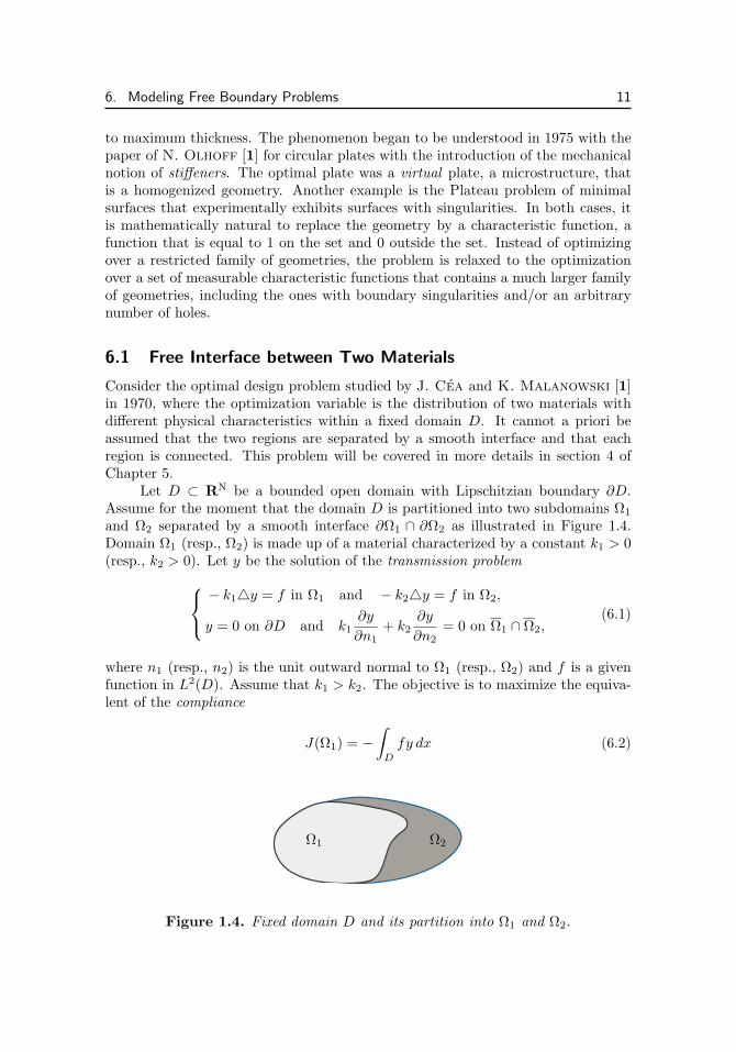
Let D ⊂ RN be a bounded open domain with Lipschitzian boundary ∂D.Assume for the moment that the domain D is partitioned into two subdomains Ω1and Ω2 separated by a smooth interface ∂Ω1 ∩ ∂Ω2 as illustrated in Figure 1.4.Domain Ω1 (resp., Ω2) is made up of a material characterized by a constant k1 > 0(resp., k2 > 0). Let y be the solution of the transmission problem

− k1y = f in Ω1 and − k2y = f in Ω2,

y = 0 on ∂D and k1∂y

∂n1+ k2

∂y

∂n2= 0 on Ω1 ∩ Ω2,

(6.1)

where n1 (resp., n2) is the unit outward normal to Ω1 (resp., Ω2) and f is a givenfunction in L2(D). Assume that k1 > k2. The objective is to maximize the equiva-lent of the compliance

J(Ω1) = −∫D

fy dx (6.2)

Ω2Ω1

Figure 1.4. Fixed domain D and its partition into Ω1 and Ω2.


over all domains Ω1 in D subject to the following constraint on the volume ofmaterial k1 which occupies the part Ω1 of D:

m(Ω1) ≤ α, 0 < α < m(D) (6.3)

for some constant α.If χ denotes the characteristic function of the domain Ω1,

χ(x) = 1 if x ∈ Ω1 and 0 if x /∈ Ω1,

the compliance J(χ) = J(Ω1) can be expressed as the infimum over the Sobolevspace H1

0 (D) of an energy functional defined on the fixed set D:

J(χ) = minϕ∈H1

0 (D)E(χ, ϕ), (6.4)

E(χ, ϕ) def=∫D

(k1 χ+ k2 (1− χ)) |∇ϕ|2 − 2χfϕdx. (6.5)

J(χ) can be minimized or maximized over some appropriate family of characteristicfunctions or with respect to their relaxation to functions between 0 and 1 that wouldcorrespond to microstructures. As in the eigenvalue problem, the objective functionis an infimum, but here the infimum is over a space that does not depend on thefunction χ that specifies the geometric domain. This will be handled by the specialtechniques of Chapter 10 for the differentiation of the minimum of a functional.

6.2 Minimal Surfaces

The celebrated Plateau’s problem, named after the Belgian physicist and profes-sor J. A. F. Plateau [1] (1801–1883), who did experimental observations on thegeometry of soap films around 1873, also provides a nice example where the geome-try is a variable. It consists in finding the surface of least area among those boundedby a given curve. One of the difficulties in studying the minimal surface problem isthe description of such surfaces in the usual language of differential geometry. Forinstance, the set of possible singularities is not known.

Measure theoretic methods such as k-currents (k-dim surfaces) were used byE. R. Reifenberg [1, 2, 3, 4] around 1960, H. Federer and W. H. Fleming [1]in 1960 (normals and integral currents), F. J. Almgren, Jr. [1] in 1965 (varifolds),and H. Federer [5] in 1969.

In the early 1950s, E. De Giorgi [1, 2, 3] and R. Caccioppoli [1] considereda hypersurface in the N -dimensional Euclidean space RN as the boundary of aset. In order to obtain a boundary measure, they restricted their attention to setswhose characteristic function is of bounded variation. Their key property is anassociated natural notion of perimeter that extends the classical surface measure ofthe boundary of a smooth set to the larger family of Caccioppoli sets named afterthe celebrated Neapolitan mathematician Renato Caccioppoli.2

2In 1992 his tormented personality was remembered in a film directed by Mario Martone, TheDeath of a Neapolitan Mathematician (Morte di un matematico napoletano).

7. Design of a Thermal Diffuser 13

Caccioppoli sets occur in many shape optimization problems (or free boundaryproblems), where a surface tension is present on the (free) boundary, such as in thefree interface water/soil in a dam (C. Baiocchi, V. Comincioli, E. Magenes,

and G. A. Pozzi [1]) in 1973 and in the free boundary of a water wave (M. Souli

and J.-P. Zolesio [1, 2, 3, 4, 5]) in 1988. More details will be given in Chapter 5.

7 Design of a Thermal DiffuserShape optimization problems are everywhere in engineering, physics, and medicine.We choose two illustrative examples that were proposed by the Canadian SpaceProgram in the 1980s. The first one is the design of a thermal diffuser to condi-tion the thermal environment of electronic devices in communication satellites; thesecond one is the design of a thermal radiator that will be described in the next sec-tion. There are more and more design and control problems coming from medicine.For instance, the design of endoprotheses such as valves, stents, and coils in bloodvessels or left ventricular assistance devices (cardiac pumps) in interventional car-diology helps to improve the health of patients and minimize the consequences andcosts of therapeutical interventions by going to mini-invasive procedures.

7.1 Description of the Physical Problem

This problem arises in connection with the use of high-power solid-state devices(HPSSD) in communication satellites (cf. M. C. Delfour, G. Payre, and J.-

P. Zolesio [1]). An HPSSD dissipates a large amount of thermal power (typ.> 50 W) over a relatively small mounting surface (typ. 1.25 cm2). Yet, its junctiontemperature is required to be kept moderately low (typ. 110C). The thermalresistance from the junction to the mounting surface is known for any particularHPSSD (typ. 1C/W), so that the mounting surface is required to be kept ata lower temperature than the junction (typ. 60C). In a space application thethermal power must ultimately be dissipated to the environment by the mechanismof radiation. However, to radiate large amounts of thermal power at moderately lowtemperatures, correspondingly large radiating areas are required. Thus we have therequirement to efficiently spread the high thermal power flux (TPF) at the HPSSDsource (typ. 40 W/cm2) to a low TPF at the radiator (typ. 0.04 W/cm2) so thatthe source temperature is maintained at an acceptably low level (typ. < 60C)at the mounting surface. The efficient spreading task is best accomplished usingheatpipes, but the snag in the scheme is that heatpipes can accept only a limitedmaximum TPF from a source (typ. max 4 W/cm2).

Hence we are led to the requirement for a thermal diffuser. This device isinserted between the HPSSD and the heatpipes and reduces the TPF at the source(typ. > 40 W/cm2) to a level acceptable to the heatpipes (typ. > 4 W/cm2). Theheatpipes then sufficiently spread the heat over large space radiators, reducing theTPF from a level at the diffuser (typ. 4 W/cm2) to that at the radiator (typ. 0.04W/cm2). This scheme of heat spreading is depicted in Figure 1.5.

It is the design of the thermal diffuser which is the problem at hand. Wemay assume that the HPSSD presents a uniform thermal power flux to the diffuser


heatpipesaddle

heatpipes

radiator to spaceschematic drawingnot to scale

thermaldiffuser high-power

solid-state diffuser

Figure 1.5. Heat spreading scheme for high-power solid-state devices.

at the HPSSD/diffuser interface. Heatpipes are essentially isothermalizing devices,and we may assume that the diffuser/heatpipe saddle interface is indeed isothermal.Any other surfaces of the diffuser may be treated as adiabatic.

7.2 Statement of the Problem

Assume that the thermal diffuser is a volume Ω symmetrical about the z-axis(cf. Figure 1.6 (A)) whose boundary surface is made up of three regular pieces:the mounting surface Σ1 (a disk perpendicular to the z-axis with center in (r, z) =(0, 0)), the lateral adiabatic surface Σ2, and the interface Σ3 between the dif-fuser and the heatpipe saddle (a disk perpendicular to the z-axis with center in(r, z) = (0, L)).

The temperature distribution over this volume Ω is the solution of the station-ary heat equation k∆T = 0 (∆T , the Laplacian of T ) with the following boundaryconditions on the surface Σ = Σ1 ∪ Σ2 ∪ Σ3 (the boundary of Ω):

k∂T

∂n= qin on Σ1, k

∂T

∂n= 0 on Σ2, T = T3 (constant) on Σ3, (7.1)

where n always denotes the outward unit normal to the boundary surface Σ and∂T/∂n is the normal derivative to the boundary surface Σ,

∂T

∂n= ∇T · n (∇T = the gradient of T ). (7.2)

The parameters appearing in (7.1) are

k = thermal conductivity (typ. 1.8W/cm×C),

qin = uniform inward thermal power flux at the source (positive constant).


The radius R0 of the mounting surface Σ1 is fixed so that the boundary surface Σ1is already given in the design problem.

For practical considerations, we assume that the diffuser is solid without in-terior hollows or cutouts. The class of shapes for the diffuser is characterized bythe design parameter L > 0 and the positive function R(z), 0 < z ≤ L, withR(0) = R0 > 0. They are volumes of revolution Ω about the z-axis generated bythe surface A between the z-axis and the function R(z) (cf. Figure 1.6 (B)), that is,

Ω def=

(x, y, z) : 0 < z < L, x2 + y2 < R(z)2. (7.3)

So the shape of Ω is completely specified by the length L > 0 and the functionR(z) > 0 on the interval [0, L].

(A) (B) (C)

z z

L Σ3

Σ2

Σ1

L

0 0

ζ

1

0y y ρ0 0 0R0 1

AR(z) S4

S3

S2

S1

D

Figure 1.6. (A) Volume Ω and its boundary Σ; (B) Surface A generatingΩ; (C) Surface D generating Ω.

Assuming that the diffuser is made up of a homogeneous material of uniformdensity (no hollow) the design objective is to minimize the volume

J(Ω) def=∫

Ωdx = π

∫ L

0R(z)2 dz (7.4)

subject to a uniform constraint on the outward thermal power flux at the interfaceΣ3 between the diffuser and the heatpipe saddle:

supp∈Σ3

−k ∂T∂z

(p) ≤ qout or k∂T

∂n+ qout ≥ 0 on Σ3, (7.5)

where qout is a specified positive constant.It is readily seen that the minimization problem (7.4) subject to the constraint

(7.5) (where T is the solution of the heat equation with the boundary conditions(7.1)) is independent of the fixed temperature T3 on the boundary Σ3. In otherwords the optimal shape Ω, if it exists, is independent of T3. As a result, from nowon we set T3 equal to 0.


7.3 Reformulation of the Problem

In a shape optimization problem the formulation is important from both the the-oretical and the numerical viewpoints. In particular condition (7.5) is difficult tonumerically handle since it involves the pointwise evaluation of the normal derivativeon the piece of boundary Σ3. This problem can be reformulated as the minimizationof T on Σ3, where T is now the solution of a variational inequality. Consider thefollowing minimization problem over the subspace of functions that are positive orzero on Σ3:

V +(Ω) def=v ∈ H1(Ω) : v|Σ3 ≥ 0

, (7.6)

infv∈V +(Ω)

∫Ω

12|∇v|2 dx−

∫Σ1

qin v dΣ +∫

Σ3

qout v dΣ. (7.7)

H1(Ω) is the usual Sobolev space on the domain Ω, and the inequality on Σ3has to be interpreted quasi-everywhere in the capacity sense. Leaving aside thosetechnicalities, the minimizing solution of (7.7) is characterized by

−k∆T = 0 in Ω, k∂T

∂n= qin on Σ1, k

∂T

∂n= 0 on Σ2,

T ≥ 0,(k∂T

∂n+ qout

)≥ 0, T

(k∂T

∂n+ qout

)= 0 on Σ3.

(7.8)

The former constraint (7.5) is verified and replaced by the new constraint

T = 0 on Σ3. (7.9)

If there exists a nonempty domain Ω of the form (7.3) such that T = 0 on Σ3, theproblem is feasible.

In this formulation the pointwise constraint on the normal derivative of thetemperature on Σ3 has been replaced by a pointwise constraint on the less de-manding trace of the temperature on Σ3. Yet, we now have to solve a variationalinequality instead of a variational equation for the temperature T .

7.4 Scaling of the Problem

In the above formulations the shape parameter L and the shape function R are notindependent of each other since the function R is defined on the interval [0, L]. Thismotivates the following changes of variables and the introduction of the dimension-less temperature y:

x → ξ1 =x

R0, y → ξ2 =

y

R0, z → ζ =

z

L, 0 ≤ ζ ≤ 1,

L =L

R0, R(ζ) =

R(Lζ)R0

,

y(ξ1, ξ2, ζ) =k

LqinT (R0ξ1, R0ξ2, Lζ),

Ddef=

(ξ1, ξ2, ζ) : 0 < ζ < 1, ξ21 + ξ22 < R(z)2.


The parameter L now appears as a coefficient in the partial differential equation

L2(∂2y

∂ξ21+∂2y

∂ξ22

)+∂2y

∂ζ2 = 0 in D

with the following boundary conditions on the boundary S = S1 ∪ S2 ∪ S3 of D:

∂y

∂νA= 1 on S1,

∂y

∂νA= 0 on S2, y = 0 on S3, (7.10)

where ν denotes the outward normal to the boundary surface S and ∂y/∂νA is theconormal derivative to the boundary surface S,

∂y

∂νA= L2

(ν1∂y

∂ξ1+ ν2

∂y

∂ξ2

)+ ν3

∂y

∂ζ.

Finally, the optimal design problem depends only on the ratio q = qout/qin throughthe constraint

∂y

∂νA+qoutqin≥ 0 on S3.

The design variables are the parameter L > 0 and the function R > 0 now definedon the fixed interval [0, 1].

7.5 Design Problem

The fact that this specific design problem can be reduced to finding a parameterand a function gives the false or unfounded impression that it can now be solvedby standard mathematical programming and numerical methods. Early work onsuch problems revealed a different reality, such as oscillating boundaries and con-vergence towards nonphysical designs. Clearly, the geometry refused to be handledby standard methods without a better understanding of the underlying physics andits inception in the modeling of the geometric variable.

At the theoretical level, the existence of solution requires a concept of conti-nuity with respect to the geometry of the solution of either the heat equation withan inequality constraint on the TPF or the variational inequality with an equalityconstraint on the temperature. The other element is the lower semicontinuity of theobjective functional that is not too problematic for the volume functional as long asthe chosen topology on the geometry preserves the continuity of the volume func-tional. For instance, the classical Hausdorff metric topology does not preserve thevolume. In the context of fluid mechanics (cf., for instance, O. Pironneau [1]), itmeans that a drag minimizing sequence of sets with constant volume may convergeto a set with twice the volume (cf. Example 4.1 in Chapter 6). A wine makingindustry exploiting the convergence in the Hausdorff metric topology could yieldmiraculous profits.

Other serious issues are, for instance, the lack of differentiability of the solutionof a variational inequality at the continuous level that will inadvertently affect thedifferentiability or the evolution of a gradient method at the discrete level. We shall


see that there is not only one topology for shapes but a whole range that selectivelypreserve some but not all of the geometrical features. Again the right choice isproblem dependent, much like the choice of the right Sobolev space in the theoryof partial differential equations.

8 Design of a Thermal RadiatorCurrent trends indicate that future communications satellites and spacecrafts willgrow ever larger, consume ever more electrical power, and dissipate larger amountsof thermal energy. Various techniques and devices can be deployed to conditionthe thermal environment for payload boxes within a spacecraft, but it is desirableto employ those which offer good performance for low cost, low weight, and highreliability. A thermal radiator (or radiating fin) which accepts a given TPF from apayload box and radiates it directly to space can offer good performance and highreliability at low cost. However, without careful design, such a radiator can be un-necessarily bulky and heavy. It is the mass-optimized design of the thermal radiatorwhich is the problem at hand (cf. M. C. Delfour, G. Payre, and J.-P. Zole-

sio [2]). We may assume that the payload box presents a uniform TPF (typ. 0.1 to1.0 W/cm2) into the radiator at the box/radiator interface. The radiating surfaceis a second surface mirror which consists of a sheet of glass whose inner surface hassilver coating. We may assume that the TPF out of the radiator/space interfaceis governed by the T 4 radiation law, although we must account also for a constantTPF (typ. 0.01 W/cm2) into this interface from the sun. Any other surfaces ofthe radiator may be treated as adiabatic. Two constraints restrict freedom in thedesign of the thermal radiator:

(i) the maximum temperature at the box/radiator interface is not to exceed someconstant (typ. 50); and

(ii) no part of the radiator is to be thinner than some constant (typ. 1 mm).

8.1 Statement of the Problem

Assume that the radiator is a volume Ω symmetrical about the z-axis (cf. Figure 1.7)whose boundary surface is made up of three regular pieces: the contact surface Σ1(a disk perpendicular to the z-axis with center at the point (r, z) = (0, 0)), thelateral adiabatic surface Σ2, and the radiating surface Σ3 (a disk perpendicular tothe z-axis with center at (r, z) = (0, L)). More precisely

Σ1 =

(x, y, z) : z = 0 and x2 + y2 ≤ R20,

Σ2 =

(x, y, z) : x2 + y2 = R(z)2, 0 ≤ z ≤ L,

Σ3 =

(x, y, z) : z = L and x2 + y2 ≤ R(L)2,

(8.1)

where the radius R0 > 0 (typ. 10 cm), the length L > 0, and the function

R : [0, L]→ R, R(0) = R0, R(z) > 0, 0 ≤ z ≤ L, (8.2)

are given (R, the field of real numbers).

8. Design of a Thermal Radiator 19

z z

L

0

Σ3

Σ2

Σ1

R00ry

Figure 1.7. Volume Ω and its cross section.

The temperature distribution (in Kelvin degrees) over the volume Ω is thesolution of the stationary heat equation

∆T = 0 (the Laplacian of T ) (8.3)

with the following boundary conditions on the surface Σ = Σ1 ∪ Σ2 ∪ Σ3 (theboundary of Ω):

k∂T

∂n= qin on Σ1, k

∂T

∂n= 0 on Σ2, k

∂T

∂n= −σεT |T |3 + qs on Σ3, (8.4)

where n denotes the outward normal to the boundary surface Σ, ∂T/∂n is thenormal derivative on the boundary surface Σ, and

∂T

∂n= ∇T · n (∇T = the gradient of T ).

The parameters appearing in (8.1)–(8.4) are

k = thermal conductivity (typ. 1.8 W/cm×C),

qin = uniform inward thermal power flux at the source (typ. 0.1 to 1.0 W/cm2),

σ = Boltzmann’s constant (5.67× 10−8 W/m2K4),

ε = surface emissivity (typ. 0.8),

qs = solar inward thermal power flux (0.01 W/cm2).

The optimal design problem consists in minimizing the volume

J(Ω) def= π

∫ L

0R(z)2 dz (8.5)

over all length L > 0 and shape function R subject to the constraint

T (x, y, z) ≤ Tf (typ. 50C), ∀(x, y, z) ∈ Σ1. (8.6)

In this analysis we shall drop the requirement (ii) in the introduction.


8.2 Scaling of the Problem

As in the case of the diffuser, it is convenient to introduce the following dimensionlesscoordinates and temperature y (see Figure 1.8):

x → ξ1 =x

R0, y → ξ2 =

y

R0, z → ζ =

z

L, 0 ≤ ζ ≤ 1,

L =L

R0, R(ζ) =

R(Lζ)R0

,

y(ξ1, ξ2, ζ) =(σεR0

k

)1/3

T (R0ξ1, R0ξ2, Lζ),

Ddef=

(ξ1, ξ2, ζ) : 0 < ζ < 1, ξ21 + ξ22 < R(z)2.

The parameter L now appears as a coefficient in the partial differential equation

L2(∂2y

∂ξ21+∂2y

∂ξ22

)+∂2y

∂ζ2 = 0 in D

with the following boundary conditions on the boundary S = S1 ∪ S2 ∪ S3 of D:

∂y

∂νA= L

[(σεR0

k

)1/3qinkR0

]on S1,

∂y

∂νA= 0 on S2,

∂y

∂νA+ Ly|y|3 = L

[(σεR0

k

)1/3qinkR0

]qsqin

on S3,

(8.7)

where ν denotes the outward normal to the boundary surface S and ∂y/∂νA is theconormal derivative to the boundary surface Σ,

∂y

∂νA= L2

(ν1∂y

∂ξ1+ ν2

∂y

∂ξ2

)+ ν3

∂y

∂ζ.

ζ ζ

1

0

S3

S2

S1

10rr

1

1

A

Σ3

Σ2

Σ1

Figure 1.8. Volume Ω and its generating surface A.

9. A Glimpse into Segmentation of Images 21

9 A Glimpse into Segmentation of ImagesThe study of the problem of linguistic or visual perceptions was initiated by severalpioneering authors, such as H. Blum [1] in 1967, D. Marr and E. Hildreth [1] in1980, and D. Marr [1] in 1982. It involves specialists of psychology, artificialintelligence, and experimentalists such as D. H. Hubel and T. N. Wiesel [1] in1962 and F. W. Campbell and J. G. Robson [1] in 1968.

In the first part of this section, we revisit the pioneering work of D. Marr

and E. Hildreth [1] in 1980 on the smoothing of the image by convolution with asufficiently differentiable normalized function as a function of the scaling parameter.We extend the space-frequency uncertainty principle to N -dimensional images. Itis the analogue of the Heisenberg uncertainty principle of quantum mechanics. Werevisit the Laplacian filter and we generalize the linearity assumption of D. Marr

and E. Hildreth [1] from linear to curved contours.In the second part, we show how shape analysis methods and the shape and

tangential calculuses can be applied to objective functionals defined on the wholecontour of an image. We anticipate Chapters 9 and 10 on shape derivatives by thevelocity method and show how they can be applied to snakes, active geodesic con-tours, and level sets (cf., for instance, the book of S. Osher and N. Paragios [1]).It shows that the Eulerian shape semiderivative is the basic ingredient behind thoserepresentations, including the case of the oriented distance function. In all cases,the evolution equation for the continuous gradient descent method is shown to havethe same structure. For more material along the same lines, the reader is referredto M. Dehaes [1] and M. Dehaes and M. C. Delfour [1].

9.1 Automatic Image Processing

The first level of image processing is the detection of the contours or the boundariesof the objects in the image. For an ideal image I : D → R defined in an opentwo-dimensional frame D with values in an interval of greys continuously rangingfrom white to black (see Figure 1.9), the edges of an object correspond to the loci ofdiscontinuity of the image I (cf. D. Marr and E. Hildreth [1]), also called “stepedges” by D. Marr [1]. As can be seen from Figure 1.9, the loci of discontinuitymay only reveal part of an object hidden by another one and a subsequent anddifferent level of processing is required. A more difficult case is the detection ofblack curves or cracks in a white frame (cf. Figure 1.10), where the function Ibecomes a measure supported by the curves rather than a function.

In practice, the frame D of the image is divided into periodically spaced cellsP (square, hexagon, diamond) with a quantized value or pixel from 256 grey lev-els. For small squares a piecewise linear continuous interpolation or higher degreeC1-interpolation can be used to remove the discontinuities at the intercell bound-aries. In addition, observations and measurements introduce noise or perturbationsand the interpolated image I needs to be further smoothed or filtered. When thecharacteristics of the noise are known, an appropriate filter can do the job (see,for instance, the use of low pass filters in A. Rosenfeld and M. Thurston [1],A. P. Witkin [1], and A. L. Yuille and T. Poggio [1]).


frame D

levels of grey I open set Ω

Figure 1.9. Image I of objects and their segmentation in the frame D.

frame D

Figure 1.10. Image I containing black curves or cracks in the frame D.

Given an ideal grey level image I defined in a fixed bounded open frame Dwe want to identify the edges or boundaries of the objects contained in the imageas shown in Figure 1.9. The edge identification or segmentation problem is a low-level processing of a real image which should also involve higher-level processings ortasks (cf. M. Kass, M. Witkin, and D. Terzopoulos [1]). Intuitively the edgescoincide with the loci of discontinuities of the image function I. At such points thenorm |∇I| of the gradient ∇I is infinite. Roughly speaking the segmentation of anideal image I consists in finding the loci of discontinuity of the function I. The ideais now to first smooth I by convolution with a sufficiently differentiable function.This operation will be followed and/or combined with the use of an edge detectoras the zero crossings of the Laplacian. In the literature the term filter often appliesto both the filter and the detector. In this section we shall make the distinctionbetween the two operations.

9.2 Image Smoothing/Filtering by Convolutionand Edge Detectors

In this section we revisit the work of D. Marr and E. Hildreth [1] in 1980 on thesmoothing of the image I by convolution with a sufficiently differentiable normalizedfunction ρ as a function of the scaling parameter ε > 0. In the second part of this


section we revisit the Laplacian filter and we generalize the linearity assumption ofD. Marr and E. Hildreth [1] from linear to curved contours.

9.2.1 Construction of the Convolution of I

Let ρ : RN → R, N ≥ 1, be a sufficiently smooth function such that

ρ ≥ 0 and∫RN

ρ(x) dx = 1.

Associate with the image I, ρ, and a scaling parameter ε > 0 the normalizedconvolution

Iε(x) def= (I ∗ ρε)(x) =1εN

∫RN

I(y) ρ(x− yε

)dy, (9.1)

where for x ∈ RN

ρε(x) def=1εN

ρ(xε

)and

∫RN

ρε(x) dx = 1. (9.2)

The function ρε plays the role of a probability density and ρε(x) dx of a probabilitymeasure. Under appropriate conditions Iε converges to the original image I asε → 0. For a sufficiently small ε > 0 the loci of discontinuity of the function Iare transformed into loci of strong variation of the gradient of the convolution Iε.When ρ has compact support, the convolution acts locally around each point in aneighborhood whose size is of order ε. A popular choice for ρ is the Gaussian withintegral normalized to one in RN defined by

GN (x) def=1

(√

2π)Ne− 1

2 |x|2 and∫RN

GN (x) dx = 1

and the normalized Gaussian of variance ε

GNε (x) =1εN

1(√

2π)Ne− 1

2 | xε |2 and∫RN

GNε (x) dx = 1. (9.3)

As noted in L. Alvarez, P.-L. Lions, and J.-M. Morel [1] in dimension N = 2,the function u(t) = G2√

2t∗ I is the solution of the parabolic equation

∂u

∂t(t, x) = ∆u(t, x), u(0, x) = I(x).

9.2.2 Space-Frequency Uncertainty Relationship

It is interesting to compute the Fourier transform F(GNε ) of GNε to make explicit therelationship between the mean square deviations of GNε and its Fourier transformF(GNε ). For ω ∈ RN, define the Fourier transform of a function f by

F(f)(ω) def=1

(√

2π)N

∫RN

f(x) e−i ω·x. (9.4)


In applications the integral of the square of f often corresponds to an energy. Weshall refer to the L2-norm of f as the energy norm and the function f2(x) as theenergy density. The Fourier transform (9.4) of the normalized Gaussian (9.3) is

F(GNε )(ω) def=1

(√

2π)N

∫RN

GNε (x) e−i ω·xdx =1

(√

2π)Ne− 1

2 |εω|2 . (9.5)

D. Marr and E. Hildreth [1] notice that there is an uncertainty relationshipbetween the mean square deviation with respect to the energy density f(x)2 and themean square deviation with respect to the energy density F(f)(ω)2 of its Fouriertransform in dimension 1 using a result of R. Bracewell [1, pp. 160–161], where heuses the constant 1/(2π) instead of 1/

√2π in the definition of the Fourier transform

that yields 1/(4π) instead of 1/2 as a lower bound to the product of the two meansquare deviations.

This uncertainty relationship generalizes to dimension N . First define thenotions of centroıd and variance with respect to the energy density f(x)2. Given afunction f ∈ L1(RN) ∩ L2(RN) and x ∈ RN, define the centroıd as

xdef=

∫RN x f(x)2 dx∫RN f(x)2 dx

(9.6)

and the variance as

〈∆x〉2 def= 〈x− x〉2 =

∫RN |x|2 f(x)2 dx∫

RN f(x)2 dx− |x|2.

Theorem 9.1 (Uncertainty relationship). Given N ≥ 1 and f ∈ W 1,1(RN) ∩W 1,2(RN) such that −ix f ∈ L1(RN) ∩ L2(RN),

〈∆x〉〈∆ω〉 ≥ N

2. (9.7)

For f = GNε

f(x) = GNε (x) =1εN

1(√

2π)Ne− 1

2 | xε |2 ⇒ 〈∆x〉2 =Nε2

2, (9.8)

f(ω) = F(GNε )(ω) =1

(√

2π)Ne− 1

2 |εω|2 ⇒ 〈∆ω〉2 =N

2 ε2(9.9)

⇒ 〈∆x〉〈∆ω〉 =N

2for GNε and F(GNε ). (9.10)

So the normalized Gaussian filter is indeed an optimal filter since it achieves thelower bound in all dimensions as stated by D. Marr and E. Hildreth [1] indimension 1 in 1980. In the context of quantum mechanics, this relationship is theanalogue of the Heisenberg uncertainty principle.


9.2.3 Laplacian Detector

One way to detect the edges of a regular object is to start from the convolution-smoothed image Iε. Given a direction v, |v| = 1, and a point x ∈ R2 an edgepoint will correspond to a local minimum or maximum of the directional derivativef(t) def= ∇Iε(x+ tv) ·v with respect to t. Denote by t such a point. Then a necessarycondition for an extremal is

D2Iε(x+ tv)v · v = 0.

The point x = x+ tv is a zero crossing following the terminology of D. Marr andE. Hildreth [1] of the second-order directional derivative in the direction v. Thuswe are looking for the pairs (x, v) verifying the necessary condition

D2Iε(x)v · v = 0 (9.11)

and, more precisely, lines or curves C such that

∀x ∈ C, ∃v(x), |v(x)| = 1, D2Iε(x)v(x) · v(x) = 0. (9.12)

This condition is necessary in order that, in each point x ∈ C, there exists a directionv(x) such that ∇Iε(x) · v is extremal.

In order to limit the search to points x rather than to pairs (x, v), the Laplaciandetector was introduced in D. Marr and E. Hildreth [1] under two assumptions:the linear variation of the intensity along the edges C of the object and the conditionof zero crossing of the second-order derivative in the direction normal to C.

Assumption 9.1 (Linear variation condition).The intensity Iε in a neighborhood of lines parallel to C is locally linear (affine).

Assumption 9.2.The zero-crossing condition is verified in all points of C in the direction of the normaln at the point, that is,

D2Iε n · n = 0 on C. (9.13)

Under those two assumptions and for a line C, it is easy to show that thepoints of C verify the necessary condition

∆Iε = 0 on C. (9.14)

Such conditions can be investigated for edges C that are the boundary Γ of asmooth domain Ω ⊂ RN of class C2 by using the tangential calculus developed insection 5.2 of Chapter 9 and M. C. Delfour [7, 8] for objects in RN, N ≥ 1, andnot just in dimension N = 2. Indeed we want to find points x ∈ Γ such that thefunction∇Iε(x)·n(x) is an extremal of the function f(t) = ∇Iε(x+t∇bΩ(x))·∇bΩ(x)in t = 0. This yields the local necessary condition D2Iε∇bΩ · ∇bΩ = D2Iε n · n = 0on Γ of Assumption 9.2. As for Assumption 9.1, its analogue is the following.


Assumption 9.3.The restriction to the curve C of the gradient of the intensity Iε is a constantvector c, that is,

∇Iε = c, c is a constant vector on C. (9.15)

Indeed the Laplacian of Iε on C can be decomposed as follows (cf. section 5.2of Chapter 9):

∆Iε = div Γ∇Iε +D2Iε n · n,

where div Γ∇Iε is the tangential divergence of ∇Iε that can be defined as follows:

div Γ∇Iε = div (∇Iε pC)|C

and pC is the projection onto C. Hence, under Assumption 9.3, div Γ(∇Iε) = 0 onC since

div Γ(∇Iε) = div (∇Iε pΓ)|Γ = div (c)|Γ = 0,

and, in view of (9.13) of Assumption 9.2, D2Iε n · n = 0 on C. Therefore

∆Iε = div Γ(∇Iε) +D2Iε n · n = 0 on C,

and we obtain the necessary condition

∆Iε = 0 on C. (9.16)

9.3 Objective Functions Defined on the Whole Edge

With the pioneering work of M. Kass, M. Witkin, and D. Terzopoulos [1]in 1988 we go from a local necessary condition at a point of the edge to a globalnecessary condition by introducing objective functionals defined on the entire edgeof an object. Here many computations and analytical studies can be simplified byadopting the point of view that a closed curve in the plane is the boundary of a setand using the whole machinery developed for shape and geometric analysis and thetangential and shape calculuses in Chapter 9.

9.3.1 Eulerian Shape Semiderivative

In this section we briefly summarize the main elements of the velocity method.

Definition 9.1.Given D, ∅ = D ⊂ RN, consider the set P(D) = Ω : Ω ⊂ D of subsets of D.The set D is the holdall or the universe. A shape functional is a map J : A → Efrom an admissible family A in P(D) with values in a topological vector space E(usually R).


Given a velocity field V : [0, τ ] ×RN → RN (the notation V (t)(x) = V (t, x)will often be used), consider the transformations

T (t,X) def= x(t,X), t ≥ 0, X ∈ RN, (9.17)

where x(t,X) = x(t) is defined as the flow of the differential equation

dx

dt(t) = V (t, x(t)), t ≥ 0, x(0, X) = X (9.18)

(here the notation x → Tt(x) = T (t, x) : RN → RN will be used). The Eulerianshape semiderivative of J in Ω in the direction V is defined as

dJ(Ω;V ) def= limt0

J(Ωt)− J(Ω)t

(9.19)

(when the limit exists in E), where Ωt = Tt(Ω) = Tt(x) : x ∈ Ω. Under appro-priate assumptions on the family V (t), the transformations Tt are homeomor-phisms that transport the boundary Γ of Ω onto the boundary Γt of Ωt and theinterior Ω onto the interior of Ωt.

9.3.2 From Local to Global Conditions on the Edge

For simplicity, drop the subscript ε of the convolution-smoothed image Iε and as-sume that the edge of the object is the boundary Γ of an open domain Ω of class C2.Following V. Caselles, R. Kimmel, and G. Sapiro [1], it is important to chooseobjective functionals that are intrinsically defined and do not depend on an arbitraryparametrization of the boundary. For instance, given a frame D = ]0, a[× ]0, b[ anda smoothed image I : D → R, find an extremum of the objective functional

E(Ω) def=∫

Γ

∂I

∂ndΓ, (9.20)

where the integrand is the normal derivative of I. Using the velocity method theEulerian shape directional semiderivative is given by the expression (cf. Chapter 9)

dE(Ω;V ) =∫

Γ

[H∂I

∂n+

∂

∂n

(∂I

∂n

)]V · ndΓ, (9.21)

where H = ∆bΩ is the mean curvature and n = ∇bΩ is the outward unit normal.Proceeding in a formal way a necessary condition would be

H∂I

∂n+

∂

∂n

(∂I

∂n

)= 0 on Γ

⇒ ∆bΩ∇I · ∇bΩ +∇(∇I · ∇bΩ) · ∇bΩ = 0

⇒ ∆bΩ∇I · ∇bΩ +D2I∇bΩ · ∇bΩ +D2bΩ∇I · ∇bΩ = 0

⇒ D2I n · n+H∂I

∂n= 0 on Γ. (9.22)


This global condition is to be compared with the local condition (9.13). It can alsobe expressed in terms of the Laplacian and the tangential Laplacian of I as

∆I −∆ΓI = 0 on Γ, (9.23)

which can be compared with the local condition (9.16), ∆I = 0. This arises from thedecomposition of the Laplacian of I with respect to Γ using the following identityfor a smooth vector function U :

divU = div ΓU +DU n · n, (9.24)

where the tangential divergence of U is defined as

div ΓU = div (U pΓ)|Γ

and pΓ is the projection onto Γ. Applying this to U = ∇I and recalling the definitionof the tangential Laplacian

∆I = div Γ∇I +D2I n · n = ∆ΓI +H∂I

∂n+D2I n · n,

where the tangential gradient ∇ΓI and the Laplace–Beltrami operator ∆ΓI aredefined as

∇ΓI = ∇(I pΓ)|Γ and ∆ΓI = div Γ(∇ΓI).

9.4 Snakes, Geodesic Active Contours, and Level Sets

9.4.1 Objective Functions Defined on the Contours

In the literature the objective or energy functional is generally made up of twoterms: one (image energy) that depends on the image and one (internal energy)that specifies the smoothness of Γ. A general form of objective functional is

E(Ω) def=∫

Γg(I) dΓ, g(I) is a function of I. (9.25)

The directional semiderivative with respect to a velocity field V is given by

dE(Ω;V ) =∫

Γ

[Hg(I) +

∂

∂ng(I)

]n · V dΓ. (9.26)

This gradient will make the snakes move and will activate the contours.

9.4.2 Snakes and Geodesic Active Contours

If a gradient descent method is used to minimize (9.25) starting from an initial curveC0 = C, the iterative process is equivalent to following the evolution Ct (boundaryof the smooth domain Ωt) of the closed curve C given by the equation

∂Ct∂t

= − [Ht gI + (∇gI · nt)] nt on Ct, (9.27)


where Ht is the mean curvature, nt is the unit exterior normal, and the right-handside of the equation is formally the “derivative” of (9.25) given by (9.26). Equa-tion (9.27) is referred to as the geodesic flow. For gI = 1 it is the motion by meancurvature

∂Ct∂t

= −Ht nt on Ct. (9.28)

9.4.3 Level Set Method

The idea to represent the contours Ct by the zero-level set of a function ϕt(x) =ϕ(t, x) for a function ϕ : [0, τ ]×RN → R by setting

Ct =x ∈ RN : ϕ(t, x) = 0

= ϕ−1

t 0

and to replace (9.27) by an equation for ϕ is due to S. Osher and J. A. Sethian [1]in 1988. This approach seems to have been simultaneously introduced in imageprocessing by V. Caselles, F. Catte, T. Coll, and F. Dibos [1] in 1993 underthe name “geometric partial differential equations” with, in addition to the meancurvature term, a “transport” term and by R. Malladi, J. A. Sethian, andB. C. Vemuri [1] in 1995 under the name “level set approach” combined with thenotion of “extension velocity.”

Let (t, x) → ϕ(t, x) : [0, τ ]×RN → R be a smooth function and Ω be a subsetof RN of boundary Γ = Ω ∩ Ω such that

int Ω =x ∈ RN : ϕ(0, x) < 0

and Γ =

x ∈ RN : ϕ(0, x) = 0

. (9.29)

Let V : [0, τ ]×RN → RN be a sufficiently smooth velocity field so that the transfor-mations Tt are diffeomorphisms. Moreover, assume that the images Ωt = Tt(Ω)verify the following properties: for all t ∈ [0, τ ]

int Ωt =x ∈ RN : ϕ(t, x) < 0

and Γt =

x ∈ RN : ϕ(t, x) = 0

. (9.30)

Assuming that the function ϕt(x) = ϕ(t, x) is at least of class C1 and that∇ϕt = 0 on ϕ−1

t 0, the total derivative with respect to t of ϕ(t, Tt(x)) for x ∈ Γyields

∂

∂tϕ(t, Tt(x)) +∇ϕ(t, Tt(x)) · d

dtTt(x) = 0. (9.31)

By substituting the velocity field in (9.18), we get

∂

∂tϕ(t, Tt(x)) +∇ϕ(t, Tt(x)) · V (t, Tt(x)) = 0, ∀Tt(x) ∈ Γt

⇒ ∂

∂tϕt +∇ϕt · V (t) = 0 on Γt, t ∈ [0, τ ]. (9.32)

This last equation, the level set evolution equation, is verified only on the boundariesor fronts Γt, 0 ≤ t ≤ τ . Can we find a representative ϕ in the equivalence class

[ϕ]Ω,V =ϕ : ϕ−1

t 0 = Γt and ϕ−1t < 0 = int Ωt,∀t ∈ [0, τ ]


of functions ϕ that verify conditions (9.29) and (9.30) in order to extend (9.32) fromΓt to the whole RN or at least almost everywhere in RN? Another possibility is toconsider the larger equivalence class

[ϕ]Γ,V =ϕ : ϕ−1

t 0 = Γt,∀t ∈ [0, τ ].

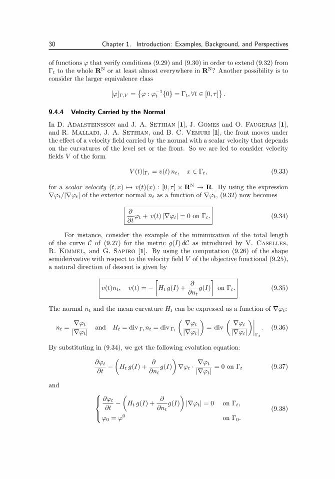
9.4.4 Velocity Carried by the Normal

In D. Adalsteinsson and J. A. Sethian [1], J. Gomes and O. Faugeras [1],and R. Malladi, J. A. Sethian, and B. C. Vemuri [1], the front moves underthe effect of a velocity field carried by the normal with a scalar velocity that dependson the curvatures of the level set or the front. So we are led to consider velocityfields V of the form

V (t)|Γt = v(t)nt, x ∈ Γt, (9.33)

for a scalar velocity (t, x) → v(t)(x) : [0, τ ] × RN → R. By using the expression∇ϕt/|∇ϕt| of the exterior normal nt as a function of ∇ϕt, (9.32) now becomes

∂

∂tϕt + v(t) |∇ϕt| = 0 on Γt. (9.34)

For instance, consider the example of the minimization of the total lengthof the curve C of (9.27) for the metric g(I) dC as introduced by V. Caselles,

R. Kimmel, and G. Sapiro [1]. By using the computation (9.26) of the shapesemiderivative with respect to the velocity field V of the objective functional (9.25),a natural direction of descent is given by

v(t)nt, v(t) = −[Ht g(I) +

∂

∂ntg(I)

]on Γt. (9.35)

The normal nt and the mean curvature Ht can be expressed as a function of ∇ϕt:

nt =∇ϕt|∇ϕt|

and Ht = div Γtnt = div Γt

(∇ϕt|∇ϕt|

)= div

(∇ϕt|∇ϕt|

)∣∣∣∣Γt

. (9.36)

By substituting in (9.34), we get the following evolution equation:

∂ϕt∂t−(Ht g(I) +

∂

∂ntg(I)

)∇ϕt ·

∇ϕt|∇ϕt|

= 0 on Γt (9.37)

and ∂ϕt∂t−(Ht g(I) +

∂

∂ntg(I)

)|∇ϕt| = 0 on Γt,

ϕ0 = ϕ0 on Γ0.

(9.38)


By substituting expressions (9.36) for nt and Ht in terms of ∇ϕt, we finally get∂ϕt∂t−[div

(∇ϕt|∇ϕt|

)g(I) +∇g(I) · ∇ϕt|∇ϕt|

]|∇ϕt| = 0 on Γt,

ϕ0 = ϕ0 on Γ0.

(9.39)

The negative sign arises from the fact that we have chosen the outward rather thanthe inward normal. The main references to the existence and uniqueness theoremsrelated to (9.39) can be found in Y. G. Chen, Y. Giga, and S. Goto [1].

9.4.5 Extension of the Level Set Equations

Equation (9.39) on the fronts Γt is not convenient from both the theoretical andthe numerical viewpoints. So it would be desirable to be able to extend (9.39) in asmall tubular neighborhood of thickness h

Uh(Γt)def=x ∈ RN : dΓt(x) < h

(9.40)

of the front Γt for a small h > 0 (dΓt , the distance function to Γt). In theory, thevelocity field associated with Γt is given by

V (t) = −[div

(∇ϕt|∇ϕt|

)g(I) +∇g(I) · ∇ϕt|∇ϕt|

]∇ϕt|∇ϕt|

on Γt. (9.41)

Given the identities (9.36), the expressions of nt and Ht extend to a neighborhoodof Γt and possibly to RN if ∇ϕt is sufficiently smooth and ∇ϕt = 0 on Γt.

Equation (9.39) can be extended to RN at the price of violating the assump-tions (9.29)–(9.30), either by loss of smoothness of ϕt or by allowing its gradient tobe zero:

∂ϕt∂t−[div

(∇ϕt|∇ϕt|

)g(I) +∇g(I) · ∇ϕt|∇ϕt|

]|∇ϕt| = 0 in RN,

ϕ0 = ϕ0 in RN .

(9.42)

In fact, the starting point of V. Caselles, F. Catte, T. Coll, and F. Dibos [1]was the following geometric partial differential equation:

∂ϕt∂t−[div

(∇ϕt|∇ϕt|

)g(I) + ν g(I)

]|∇ϕt| = 0 in RN,

ϕ0 = ϕ0 in RN(9.43)

for a constant ν > 0 and the function g(I) = 1/(1+|∇I|2). They prove the existence,in dimension 2, of a viscosity solution unique for initial data ϕ0 ∈ C([0, 1]× [0, 1])∩W 1,∞([0, 1]× [0, 1]) and g ∈W 1,∞(R2).


9.5 Objective Function Defined on the Whole Image

9.5.1 Tikhonov Regularization/Smoothing

The convolution is only one approach to smoothing an image I ∈ L2(D) defined ina frame D. Another way is to use the Tikhonov regularization: given ε > 0, find afunction Iε ∈ H1(D) that minimizes the objective functional

Eε(ϕ) def=12

∫D

ε|∇ϕ|2 + |ϕ− I|2 dx,

where the value of ε can be suitably adjusted to get the desired degree of smooth-ness. The minimizing function Iε ∈ H1(D) is solution of the following variationalequation:

∀ϕ ∈ H1(D),∫D

ε∇Iε · ∇ϕ+ (Iε − I)ϕdx = 0. (9.44)

The price to pay now is that the computation is made on the whole image.This can be partly compensated by combining in a single operation or level of

processing the smoothing of the image with the detection of the edges. To do thatD. Mumford and J. Shah [1] in 1985 and [2] in 1989 introduced a new objectivefunctional that received a lot of attention from the mathematical and engineeringcommunities.

9.5.2 Objective Function of Mumford and Shah

Given a grey level ideal image in a fixed bounded open frame D we are looking for anopen subset Ω of D such that its boundary reveals the edges of the two-dimensionalobjects contained in the image of Figure 1.9.

Definition 9.2.Let D be a bounded open subset of RN with Lipschitzian boundary.

(i) An image in the frame D is specified by a function I ∈ L2(D).

(ii) We say that Ωjj∈J is an open partition of D if Ωjj∈J is a family of disjointconnected open subsets of D such that

mN (∪j∈JΩj) = mN (D) and mN (∂ ∪j∈J Ωj) = 0,

where mN is the N -dimensional Lebesgue measure. Denote by P(D) thefamily of all such open partitions of D.

The idea behind the formulation of D. Mumford and J. Shah [1] in 1985is to do a Tikhonov regularization Iε,j ∈ H1(Ωj) of I on each element Ωj of thepartition and then minimize the sum of the local minimizations over Ωj over all open


partitions of the image D: find an open partition P = Ωjj∈J in P(D) solution ofthe minimization problem

infP∈P(D)

∑j∈J

infϕj∈H1(Ωj)

∫Ωj

ε|∇ϕj |2 + |ϕj − I|2 dx (9.45)

for some fixed constant ε > 0. Observe that without the condition mN (∪j∈JΩj) =mN (D) the empty set would be a solution of the problem.

The question of existence requires a more specific family of open partitions ora penalization term that controls the “length” of the interfaces in some sense:

infP∈P(D)

∑j∈J

infϕj∈H1(Ωj)

∫Ωj

ε|∇ϕj |2 + |ϕj − I|2 dx+ cHN−1(∂ ∪j∈J Ωj) (9.46)

for some c > 0, where HN−1 is the Hausdorff (N − 1)-dimensional measure. Equiv-alently, we are looking for

Ω = ∪j∈JΩj open in D such that χΩ = χD a.e. in D

(χΩ and χD, characteristic functions) solution of the following minimization problem:

infΩ open ⊂DχΩ=χD a.e.

infϕ∈H1(Ω)

∫Ωε|∇ϕ|2 + |ϕ− I|2 dx+ cHN−1(∂Ω). (9.47)

In general, the Hausdorff measure is not a lower semicontinuous functional. Soeither the (N − 1)-Hausdorff measure HN−1 is relaxed to a lower semicontinuousnotion of perimeter or the minimization problem is reformulated with respect toa more suitable family of open domains and/or a space of functions larger thanH1(Ω).

Another way of looking at the problem would be to minimize the number J ofconnected subsets of the open partition, but this seems more difficult to formalize.

9.5.3 Relaxation of the (N − 1)-Hausdorff Measure

The choice of a relaxation of the (N − 1)-Hausdorff measure HN−1 is critical. Herethe finite perimeter of Caccioppoli (cf. section 6 in Chapter 5) reduces to theperimeter of D since the characteristic function of Ω is almost everywhere equalto the characteristic function of D. However, the relaxation of HN−1(∂Ω) to the(N−1)-dimensional upper Minkowski content by D. Bucur and J.-P. Zolesio [8]is much more interesting and in view of its associated compactness theorem (cf.section 12 in Chapter 7) it yields a unique solution to the problem.

9.5.4 Relaxation to BV-, Hs-, and SBV-Functions

The other avenue to explore is to reformulate the minimization problem with respectto a space of functions larger than H1(Ω).

One possibility is to use functions with possible jumps, such as functions ofbounded variations. In dimension 1, the BV-functions can be decomposed into an


absolutely continuous function in W 1,1(0, 1) plus a jump part at a countable numberof points of discontinuity. Such functions have their analogue in dimension N . Withthis in mind one could consider the penalized objective function

JBV(ϕ) def=∫D

|ϕ− I|2 dx+ ε‖ϕ‖2BV(D), (9.48)

which is similar to the Tikhonov regularization when rewritten in the form

JH1(ϕ) def=∫D

|ϕ− I|2 dx+ ε‖ϕ‖2H1(D) =∫D

(1 + ε)|ϕ− I|2 dx+ ε|∇ϕ|2 dx,

where we square the penalization term to make it differentiable. Unfortunately, thesquare of the BV-norm is not differentiable.

Going back to Figure 1.9, assume that the triangle T has an intensity of 1,the circle C has an intensity of 2/3, and the remaining part of the square S hasan intensity of 1/3. The remainder of the image is set equal to 0. Then the imagefunctional is precisely

I(x) = χT (x) +23χC +

13χS\(T∪C).

We know from Theorem 6.9 in section 6.3 of Chapter 5 that the characteristicfunction of a Lipschitzian set is a BV-function. Therefore, if we minimize theobjective functional (9.48) over all ϕ ∈ BV(D), we get exactly ϕ = I. If we insiston formulating the minimization problem over a Hilbert space as for the Tikhonovregularization, the norm of the penalization term can be chosen in the space Hs(D)for some s ∈ (0, 1]:

JHs(ϕ) def=∫D

|ϕ− I|2 dx+ ε ‖ϕ‖2Hs(D).

For 0 < s < 1/2, the norm is given by the expression

‖ϕ‖Hs(D)def=∫D

dx

∫D

dy|ϕ(y)− ϕ(x)|2|y − x|N+2s

and the relaxation is very close to the one in BV(D) since BV(D)∩L∞(D) ⊂ Hs(D),0 < s < 1/2 (cf. Theorem 6.9 (ii) in Chapter 5).

However, as seducing as those relaxations can be, it is not clear that the ob-jectives of the original formulation are preserved. Take the BV-formulation. It isimplicitly assumed that there are clean jumps across the interfaces. This is true indimension 1, but not in dimension strictly greater than 1 as explained in L. Am-

brosio [1], where he points out that the distributional gradient of a BV-functionwhich is a vector measure has three parts: an absolutely continuous part, a jumppart, and a nasty Cantor part. The space BV(D) contains pathological functions ofCantor–Vitali type that are continuous with an approximate differential 0 almosteverywhere, and this class of functions is dense in L2(D), making the infimum of


JBV over BV(D) equal to zero without giving information about the segmentation.To get around this difficulty, he introduces the smaller space SBV(D) of functionswhose distributional gradient does not have a Cantor part. He considers the math-ematical framework for the minimization of the objective functional

J(ϕ,K) def=∫D\K

|ϕ− I|2 + ε|∇ϕ|2 dx+ cHN−1(K)

with respect to all closed sets K ⊂ Ω and ϕ ∈ H1(Ω\K), where I ∈ L∞(D). Thisproblem makes sense and has a solution in SBV(D) when K is replaced by the setSϕ of points where the function ϕ ∈ SBV(D) has a jump, that is,

J(ϕ) def=∫D

|ϕ− I|2 + ε|∇ϕ|2 dx+ cHN−1(Sϕ),

that turns out to be well-defined on SBV(D).

9.5.5 Cracked Sets and Density Perimeter

The alternate avenue to explore is to reformulate the minimization problem withrespect to a more suitable family of open domains (cf. section 15 of Chapter 7).

An additional reason to do that would be to remove the term on the length ofthe interface. When a penalization on the length of the segmentation is included,long slender objects are not “seen” by the numerical algorithms since they havetoo large a perimeter. In order to retain a segmentation of piecewise H1-functionswithout a perimeter term, M. C. Delfour and J.-P. Zolesio [38] introduced thefamily of cracked sets (see Figure 1.11) that yields a compactness theorem in theW 1,p-topology associated with the oriented distance function (cf. Chapter 7).

Figure 1.11. Example of a two-dimensional strongly cracked set.

The originality of this approach is that it does not require a penalizationterm on the length of the segmentation and that, within the set of solutions,there exists one with minimum density perimeter as defined by D. Bucur andJ.-P. Zolesio [8].


Theorem 9.2. Let D be a bounded open subset of RN and α > 0 and h > 0 be realnumbers.3 Consider the families

F(D,h, α) def=

Ω ⊂ D :Γ = ∅ and ∀x ∈ Γ, ∃d, |d| = 1,

such that inf0<t<h

dΓ(x+ td)t

≥ α

,

Ch,αb (D) def= bΩ : Ω ∈ F(D,h, α) ,

(9.49)

Fs(D,h, α) def=

Ω ⊂ D :Γ = ∅ and ∀x ∈ Γ, ∃d, |d| = 1,

such that inf0<|t|<h

dΓ(x+ td)|t| ≥ α

,

(Ch,αb )s(D) def= bΩ : Ω ∈ Fs(D,h, α) .

(9.50)

Then Ch,αb (D) and (Ch,αb )s(D) are compact in W 1,p(D), 1 ≤ p < ∞, where dΓ isthe distance function to the boundary of Ω.

In view of the above compactness, it can be shown that there exists a solutionto the following minimization problem:

infΩ∈F(D,h,α)

Ω open ⊂D,mN (Ω)=mN (D)

infϕ∈H1(Ω)

∫Ωε |∇ϕ|2 + |ϕ− f |2 dx. (9.51)

Cracked sets form a very rich family of sets with a huge potential that is notyet fully exploited in the image segmentation problem. Indeed, they can be usednot only to partition the frame of an image but also to detect isolated cracks andpoints provided an objective functional sharper than the one of Mumford and Shahis used. For instance, in view of the connection between image segmentation andfracture theory hinted at in J. Blat and J.-M. Morel [1], the theory may havepotential applications in problems related to the detection of fractures or cracksor fracture branching and segmentation in geomaterials (cf. K. B. Broberg [1]),but this is way beyond the scope of this book. Some initial considerations aboutthe numerical approximation of cracked sets can be found in M. C. Delfour andJ.-P. Zolesio [41].

10 Shapes and Geometries: Backgroundand Perspectives

10.1 Parametrize Geometries by Functions or Functionsby Geometries?

In the buckling of the column and in the design of the thermal diffuser and thethermal radiator the geometry was a volume of revolution generated by rotationaround the z-axis of the hypograph between the axis and the graph of the function

3In view of the fact that the distance function dΓ is Lipschitzian with constant 1, we necessarilyhave 0 < α ≤ 1.

10. Shapes and Geometries: Background and Perspectives 37

defined in a variable interval [0, L]. They are examples of sets parametrized by func-tions or scalars. A well-documented weakness of this approach is that numericalcomputations of optimal shapes often yield boundary oscillations. This is typicalof the parametrization of the boundary by a function. It provides a good controlof the displacement in the direction normal to the graph but little control in thetangential direction.

Extending this approach to sets locally defined by several graphs becomestricky. For instance, it is not possible to represent a sphere or a torus from a bi-Lipschitzian mapping from some domain in the plane unless we replace the plane bya surface with facets as illustrated in Figure 1.12 for a ball (cf. M. C. Delfour [8]for the construction of a surface with facets from a C1,1-surface). Moreover, thesurface with facets of Figure 1.12 is closely associated with the ball and would notbe appropriate for a torus.

Figure 1.12. Example of a surface with facets associated with a ball.

Another family of function-parametrized sets is the family of images of a fixedset by a family of homeomorphisms or diffeomorphisms. This can be advantageousin problems where it is desirable to work with a fixed mesh of the original do-main, thus avoiding remeshing the domain at each step of the optimization process.Function-parametrized sets are also used in the identification of objects (cf., for in-stance, the school of R. Azencott, A. Trouve, and L. Younes). This approach can betraced back to R. Courant and D. Hilbert [1] in 1953 and the construction ofCourant metrics and complete metric spaces of images of a fixed closed or crack-freeopen set by A. M. Micheletti [1] in 1972. This approach is less interesting inoptimization problems where the topology of the set is part of the unknown fea-tures of the set. Indeed, the images of a fixed set by an homeomorphism cannotchange the topology of the fixed set. For instance, it cannot create holes that arenot present in the fixed set.

The example of the distribution of two materials in a fixed domain is genericof problems where the topology of the set is part of the unknowns. The variablechosen to represent the set is the characteristic function χA, a function parametrizedby the set A. As such, arbitrary geometries that are only measurable can be used asindependent variables. The topology (for instance, the number of holes) is not fixeda priori and extremely complex design can be obtained. Moreover, the underlying


Lp-spaces where the characteristic functions naturally live induce a metric

ρ([A1], [A2]) = ‖χA2 − χA2‖Lp(D)

on the family of equivalence classes of Lebesgue measurable subsets of a boundedmeasurable holdall D. This type of topology has been used in the proof of theMaximum Principle by Pontryagin and later by Ekeland.

Other examples of set-parametrized functions include the uniformly Lipschitz-ian distance function dA to a set A. The family of such functions for subsets of aholdall D, D bounded open, can be considered as a family of functions in C0(D) orW 1,p(D). For instance, the metric

ρ([A1], [A2]) = ‖dA2 − dA2‖C0(D)

([A] is the equivalence class of all subsets of D with the same closure) coincideswith the ecart mutuel between two sets introduced by D. Pompeiu [1] in his thesispresented in Paris in March 1905 that was studied in more detail by F. Hausdorff

[2, “Quellenangaben,” p. 280, and Chap. VIII, sect. 6] in 1914. Unfortunately thatmetric does not preserve the volume functional, but the norm can be changed toobtain the new metric

ρ([A1], [A2]) = ‖dA2 − dA2‖W 1,p(D)

that preserves the volume functional.Another example of a set-parametrized function is the support function

σA(x) def= supa∈A

a · x

of convex analysis. Here the equivalence classes are

[A] def=B ⊂ D : co B = co A

,

that is, sets with the same closed convex hull. The associated metric is

ρ([A1], [A2]) = ‖σA2 − σA2‖C0(B),

where B is the unit open ball in RN (cf. M. C. Delfour and J.-P. Zolesio [17]).The general pattern that emerges from the last three examples is the following

one. Choose a fixed holdall D and let A denote a variable set in D. Select a familyof set parametrized functions fA and let

[A] def=B ⊂ RN : fA = fB

be the associate equivalence class. Finally, assume that the family of functions fAis contained in a Banach space B(D). Choose as a metric

ρ([A1], [A2]) = ‖fA2 − fA2‖B(D).

This approach will be detailed in Chapters 5, 6, and 7 for the characteristic functionχA, the distance function dA, and the oriented distance function bA, but many otherset-parametrized functions can be used according to the requirements of the problemat hand.


10.2 Shape Analysis in Mechanics and Mathematics

The terminology shape analysis has been introduced independently in at least twodifferent contexts: continuum mechanics and mathematical theory of partial differ-ential equations (cf., for instance, E. J. Haug and J. Cea [1]).

In continuum mechanics, shape analysis encompasses contributions to struc-tural mechanics of elastic bodies such as beams, plates, shells, arches, and trusses.In such problems, the objective is to optimize the compliance, e.g., the work of theapplied loadings, by choosing the design parameters of the structure. Many of theearly contributions are in dimension 2 and complete analytical solutions are oftenprovided. Yet, it is not always easy to distinguish between a shape optimizationproblem, such as the shape of a two-dimensional plate, and a distributed param-eter problem, such as the optimal thickness of that plate. The thickness that isoften considered as a shape parameter is really a distributed parameter over thetwo-dimensional domain, which also specifies the plate. When the thickness goes tozero in some parts of the plate, holes are created and induce changes in the topologyand the shape of the associated two-dimensional domain. This naturally leads totopological optimization, which deals with the connectivity of a domain, the numberof holes, the fractal dimension of the boundary, and ultimately the appearance ofa microstructure. This was exemplified by K.-T. Cheng and N. Olhoff [2]’scelebrated optimization of the compliance of the circular plate with respect to itsthickness under prescribed loading and a constraint on the volume of material.Such questions have received a lot of attention in specific cases and have beenanalyzed by homogenization methods or Γ-convergence (cf., for instance, F. Mu-

rat and L. Tartar [1], the conference proceedings edited by M. Bendsøe andC. A. Mota Soares [1], the book by M. Bendsøe [1], and the book edited byA. Cherkaev and R. Kohn [1] that contains a selection of translations of keypapers written in French or Russian). However, many fundamental questions stillremain open. For instance, how does such an analysis affect the validity of theunderlying mechanical or physical models?

For convenience we shall refer to this viewpoint as the compliance analysis thatgenerally involves the extremum of the minimum of an energy or work functionalwith respect to some design parameters.

In the mathematical theory of partial differential equations, the analysis dealtwith the sensitivity of the solution of boundary value problems with respect tothe shape of the geometric domain on which the partial differential equation isdefined. This was done for different applications, including free boundary problems,noncylindric problems,4 and shape identification problems. This shape sensitivityanalysis was simultaneously developed for the solution of the partial differentialequation and for shape functionals depending on their solution.

In that context, the compliance analysis becomes a special case that, quiteremarkably, does not require the shape sensitivity analysis of the solution of theassociated partial differential equation (cf. section 2 of Chapter 10). This important

4A cylindric problem is a partial differential equation where the geometric domain is fixed andindependent of the time variable. A noncylindric problem is a partial differential equation wherethe geometric domain changes with time.


simplification arises from the fact that the compliance is the minimum of an energyor work functional. An historical example that also benefits from this property isthe shape derivative of the first eigenvalue of the plate studied at the beginning ofthe 20th century by J. Hadamard [1]. As for the compliance, the shape sensitivityanalysis of the first eigenfunction is not required even when the first eigenvalue isrepeated. This follows from the fact that the first eigenvalue can be expressed asa minimum through Rayleigh’s quotient or G. Auchmuty [1]’s dual variationalprinciple.

Shape sensitivity analysis deals with a larger class of shape functionals (e.g.,minimal drag, noise reduction) and partial differential equations (e.g., the waveequation, viscous or non-Newtonian fluids), where variational energy functionalsare usually not available and for which the compliance analysis is no longer appli-cable. Yet, the shape sensitivity analysis of the solution of the partial differentialequation can again be avoided by incorporating the partial differential equationinto a Hamiltonian or Lagrangian formulation. As in control theory, this yieldsa partial differential equation for the adjoint state that is coupled with the initialpartial differential equation or state equation. A precise mathematical justificationof this approach can be given when the Lagrangian has saddle points and the shapederivative can be obtained from theorems on the differentiability of saddle pointswith respect to a parameter even when the saddle point solution is not unique(cf. section 5 in Chapter 10).

The shape sensitivity analysis through a family of diffeomorphisms which pre-serve the smoothness of the images of a fixed domain is primarily a local analysis.It is used to establish continuity, to define derivatives, or to optimize in a narrowclass of domains with fixed regularities and topologies: it cannot create holes orsingularities that were not present in the initial domain. Consider the problem offinding the best location and shape of a hole of given volume in a homogeneouselastic plate to optimize the compliance or some other criterion under a given load-ing. The expectation is that the presence of the hole would improve the complianceover a homogeneous plate without holes. This problem has its analogue in controltheory, for instance the optimal placement of sensors and actuators for the con-trol and stabilization of large flexible space structures or flexible arms of robots.Another important example is the localization of sensors and actuators to achievenoise reduction in structures. The optimal placement is usually an integral part ofthe control synthesis.

In the early 1970s J. Cea, A. J. Gioan, and J. Michel [1] proposed tointroduce relaxed problems in which the optimal domain (here an optimal hole, theoptimal location of the support of the optimal control) was systematically replacedby a density function ranging between zero and one and that would hopefully be acharacteristic function (a bang bang control) in the optimal regime. Furthermore,in order to work on a fixed domain D without holes, they replaced the holes bya very weak elastic material. This changed the original topological optimizationproblem into the identification of distributed coefficients over the fixed domain D.Equivalently, this identification problem reduces to finding the optimal distributionof two materials for a transmission equation in D under a volume constraint on oneof the two materials. Under appropriate conditions, the solution of this problem isa characteristic function, even when the space of distributed parameters is relaxed


to the closed convex hull of the set of characteristic functions (cf. Chapter 5).This general technique can also be used to study the continuity of the solution ofthe homogeneous Dirichlet boundary value problems with respect to the domainΩ, by introducing a transmission problem over a fixed domain D and letting thedistributed coefficient go to infinity in the complement of Ω with respect to D. Ofcourse, the coefficient over the complement of Ω could be replaced by a Lagrangemultiplier, thus providing a formulation over the fixed domain D. This is one ofthe many ways to make the domain fictitious and avoid dealing directly with thegeometry (cf. R. Glowinski, T.-W. Pan, and J. Periaux [1]).

10.3 Characteristic Functions: Surface Measure andGeometric Measure Theory

The main advantage of the relaxation to a characteristic function in the formulationof problems involving a domain integral and/or a volume constraint on Lebesguemeasurable sets is that the unknown set is completely described by a single functioninstead of a family of local diffeomorphisms.

Yet, such measurable sets can be quite unstructured. For example, in problemsinvolving a surface tension on the free boundary of a fluid or on the interface be-tween two fluids, the domain must have a locally finite boundary measure. Anotherexample is when the objective functional is a function of the normal derivative of thestate variable along the boundary (e.g., a flow or a thermal power flux through theboundary). In both cases the use of characteristic functions is limited by the factthat they are not differentiable on the boundary of the set and cannot be readilyused to describe very smooth domains.

Fortunately, there is enough latitude to make sense of a locally finite boundarymeasure for sets for which the characteristic function is of bounded variation; thatis, its gradient is a vector of bounded measures. Such sets are known as Caccioppolior finite perimeter sets. They were a key ingredient in the contribution of E. DeGiorgi to the theory of minimal surfaces in the 1950s, since the norm of that vectormeasure (which is the total variation of the characteristic function) turns out to be arelaxation of the boundary measure or “perimeter” of the set. To get a compactnessresult for a family of Caccioppoli sets it is sufficient to put a uniform bound on theirperimeters. This field of activities is known as geometric measure theory, and itstools have been used very successfully in the theory of free and moving boundaryproblems. Even though it came rather late to shape analysis, this material is bothimportant and fundamental.

10.4 Distance Functions: Smoothness, Normal, and Curvatures

Another set-parametrized function that plays a role similar to the characteristicfunction is the distance function between closed subsets of a fixed holdall5 D ofRN. The “ecart mutuel” between two sets was introduced by D. Pompeiu [1] in

5This set D will play several roles in this book. It is the universe in which the variable subsetslive. It will often be referred to as the underlying holdall. In other circumstances it will have apurely technical role, much like the control volume in fluid mechanics.


his thesis presented in Paris in March 1905. This is the first example of a metric be-tween two sets in the literature. It was studied in more detail by F. Hausdorff [2,“Quellenangaben,” p. 280, and Chap. VIII, sect. 6] in 1914. The Pompeiu–Hausdorffmetric between two sets corresponds to the uniform norm of the difference of theirrespective distance functions. For most applications it is not a very interestingtopology since the volume functional is not continuous in that topology. The con-tinuity of the volume functional can be recovered by replacing the uniform normby the W 1,p-norm since the characteristic function of the closure of the set can beexpressed in terms of the gradient of the distance function.

In 1951, H. Federer [1] introduced the family of sets of positive reach andgave a first access to curvatures from the distance function in much the same spiritas the perimeter from the characteristic function. They are sets for which the pro-jection onto the set is unique in a neighborhood of the set. Since the projectioncan be expressed in terms of the gradient of the square of the distance function,this is equivalent to requiring that the square of the distance function be C1,1 ina neighborhood of the set. Since the gradient of the distance function has a jumpdiscontinuity at the boundary of the set, he managed to recover from the distancefunction the curvature measures of the boundary and made sense of the classicalSteiner formula for sets with positive reach.

The jump discontinuity of the characteristic function across the boundarycan be bypassed by going to the oriented distance function. For smooth domainsthis function is quite remarkable since it inherits the same degree of smoothnessin a neighborhood of the boundary as the boundary itself. Then the gradient,the Hessian matrix, and the higher-order derivatives in the neighborhood of theboundary can be used to characterize and compute normals, curvatures, and theirderivatives along the boundary. This correspondence remains true for domainsof class C1,1. The gradient of the oriented distance function coincides with theoutward unit normal on the boundary. This implicit orientation is at the origin ofthe terminology oriented distance function that was introduced by M. C. Delfour

and J.-P. Zolesio [17] in 1994 to distinguish it from the algebraic distance functionto a submanifold that can be defined only in terms of some discriminating criterionthat distinguishes between what is above and what is below the submanifold. Thisis not always possible, while the oriented distance function to a set is always well-defined. The restriction of the Hessian matrix of the oriented distance function tothe boundary coincides with the second fundamental form of differential geometry.Its eigenvalues are zero and the principal curvatures of the boundary.

A nice relaxation of the curvatures is obtained by considering sets for whichthe elements of the Hessian matrix of the oriented distance function are boundedmeasures. They are called sets of locally bounded curvature (cf. M. C. Delfour

and J.-P. Zolesio [17, 32]). To get a compactness result, it is sufficient to put auniform bound on the total variation of the gradient (the elements of the Hessianmatrix are bounded measures).

The oriented distance function also provides a framework to compare thesmoothness of sets ranging from arbitrary sets with a nonempty boundary to setsof class C∞ via the smoothness of the oriented distance function in a neighborhoodof the boundary of the set. As a result Sobolev spaces can be used to introduce the


notion of a Sobolev domain, which becomes intertwined with the classical notion ofCk-domains.

10.5 Shape Optimization: Compliance Analysisand Sensitivity Analysis

As in the vector space case, optimization and control problems with respect togeometry are of various degrees of difficulty. When the objective functional does notdepend on the solution of a state equation or variational inequality defined on thevariable domain, it is sufficient to invoke compactness and continuity arguments. Inspecial cases such as the optimization of the compliance or of the first eigenvalue, theproblem can be transformed into the optimization of an objective functional thatis itself the minimum of some appropriate functional defined on a fixed functionspace. There a direct study of the dependence of the solution of the state equationwith respect to the underlying domain can be bypassed. In the general case, a stateequation constraint has to be handled very carefully from both the mathematicaland the application viewpoints. When the analysis can be restricted to families ofLipschitzian or convex domains, it is usually possible to give a meaning and provethe continuity of the solution of the state equation with respect to the underlyingvarying domain.

When families of arbitrary bounded open domains are considered, new phe-nomena can occur. As the domains converge in some sense, the correspondingsolutions may only converge in a weak sense to the solution of a different type ofstate equation over the limit domain: boundary conditions may no longer be sat-isfied, strange terms6 may occur on the right-hand side of the equation, etc. Insuch cases, it is often a matter of modeling of the physical or technological phe-nomenon. Is it natural to accept a generalized solution or a relaxed formulationof the state equation or should the family of domains be sufficiently restricted topreserve the form of the original state equation and maintain the continuity of thesolution with respect to the domain? The most suitable relaxation is not necessarilythe most general mathematical relaxation. It must always be compatible with thephysical or technological problem at hand. Too general a relaxation of the problemor too restrictive conditions on the varying domains can yield completely unsatis-factory solutions however nice the underlying mathematics are. A good balance ofmathematical, physical, and engineering intuitions is essential.

The study of the shape continuity of the solution of the partial differentialequation is also of independent mathematical interest. In the literature, this issuehas been addressed in various ways. Some authors simply introduce a stabilityassumption that essentially says that the limiting domain is such that continuityoccurs. Others introduce a set of more technical assumptions that correspond to aminimal set of conditions to make the crucial steps of the proof of the continuitywork. On the constructive side the really challenging issue is to characterize thefamilies of domains for which the continuity holds.

6Cf., for instance, D. Cioranescu and F. Murat [1, 2].


Many authors have constructed compact families for that purpose. For in-stance the Courant metric topology was used by A. M. Micheletti [1] in 1972 forCk-domains, the uniform cone condition by D. Chenais [1] in 1973 for uniformlyLipschitzian domains, and other metric topologies by F. Murat and J. Simon [1]in 1976 for Lipschitzian domains.

More general capacity conditions were introduced after 1994 by D. Bucur andJ.-P. Zolesio [5] in order to obtain compact subfamilies of domains with respect tothe complementary Hausdorff topology and control the curvature of the boundariesof the domains. In dimension 2 they recover the nice result of V. Sverak [2]in 1993, which involves a uniform bound on the number of connected componentsof the complement of the sets. Intuitively the capacity conditions are such that,locally, the complement of the domains in the chosen family has “enough capacity”to preserve the homogeneous Dirichlet boundary condition in the limit. Yet, thecapacity conditions might not be easy to use in a specific example. So D. Bucur

and J.-P. Zolesio [1, 5] introduced a simpler geometric constraint, called the flatcone condition, under which the continuity and compactness results still hold. Thisgeneralizes the uniform cone property to a much larger class of open domains. Allthis will be further generalized in section 9 of Chapter 8.

10.6 Shape Derivatives

For functionals defined on a family of domains, it is important to distinguish betweena function with values in a topological vector space over a fixed domain and afunction such as the solution of a partial differential equation that lives in a Sobolevspace defined on the varying domain. In the latter case special techniques have tobe used to transport the solution onto a fixed domain or to first embed the varyingdomains into a fixed holdall D, extend the solutions to D, and enlarge the Sobolevspace to a large enough space of functions defined over the fixed holdall D. In bothcases the function is defined over a family of domains or sets belonging to someshape space which is generally nonlinear and nonconvex. Thus, defining derivativeson those spaces is more related to defining derivatives on differentiable manifoldsthan in vector spaces.

It is perhaps for groups of diffeomorphisms that the most complete theory ofshape derivatives is available. This material will be covered in detail in Chapters 2,3, and 9, but it is useful to briefly introduce the main ideas and definitions here.Given a Banach space Θ of mappings from a fixed open holdall D ⊂ RN into RN,first consider the group of diffeomorphisms

F(Θ) def=F : D → D : F − I ∈ Θ and F−1 − I ∈ Θ

.

Then consider the images of a fixed domain Ω0 in D by F(Θ):

X (Ω0) def= F (Ω0) : ∀F ∈ F(Θ) .

They can be identified with the quotient group

F(Θ)/G(Ω0), G(Ω0) def= F ∈ F(Θ) : F (Ω0) = Ω0


of diffeomorphisms of D. For the specific choices of D, Θ, and Ω0 that are ofinterest, this quotient group can be endowed with the so-called Courant metric tomake it a complete metric space. This metric space is neither linear nor convex.

For unconstrained domains (D = RN) and “sufficiently small” elements θ ∈ Θ,transformations of the form F = I + θ belong to F(Θ) and hence perturbations ofthe identity (i.e., of Ω0) can be chosen in the vector space Θ. This makes it possibleto define directional derivatives and speak of Gateaux and Frechet differentiabilitywith respect to Θ as in the classical case of functions defined on vector spaces.However, this approach does not extend to submanifolds D of RN or to domainsthat are constrained in one way or another (e.g., constant volume, perimeter, etc.).

In the unconstrained case, we get an infinite-dimensional differentiable man-ifold structure on the quotient group F(Θ)/G(Ω0) and the tangent space to F(Θ)is the whole linear space Θ. As a result ideas and techniques from differential ge-ometry are readily applicable. For instance, the continuity in I (i.e., at Ω0) canbe characterized by the continuity along one-dimensional flows of velocity fields inF(Θ) through the point I (that is, I(Ω0) = Ω0). This suggests defining a notion ofdirectional derivative along one-dimensional flows associated with “velocity fields”V which keep the flows inside D. When D is a smooth submanifold of RN suchvelocities are tangent to D and the set of all such velocities has a vector space struc-ture. This key property generalizes to other types of holdalls. So it is possible todefine directional derivatives and speak of shape gradient and shape Hessian withrespect to the associated vector space of velocities. This second approach has beenknown in the literature as the velocity method. Another very nice property of thatmethod is that perturbations of the identity, as previously defined in the uncon-strained case, can be recovered by a special choice of velocity field, thus creating acertain unity in the methodology.

The concept of topological derivative was introduced by J. Sokolowski andA. Zochowski [1] for problems where the knowledge of the optimal topology ofthe domain is important. It gives some sensitivity of a shape functional to thepresence of a small hole at a point of the domain as the size of that hole goes tozero. For a domain integral, that is, the integral of a locally Lebesgue integrablefunction, this derivative is the negative of the classical set-derivative which is equalto the function at almost every point. This is a direct consequence of the Lebesguedifferentiation theorem. So, at least in its simplest form, this approach aims atextending the classical concept of set-differentiation as the inverse of integrationover sets.

This type of derivative becomes more intricate as we look at the sensitivity ofthe solution of a boundary value problem or at shape functionals which are functionsof that solution. For functions that are the integrals of an integrable function withrespect to a Radon measure, the Lebesgue differentiation extends in the form of theLebesgue–Besicovitch differentiation theorem, which says that the set-derivative ofthat integral is again equal to the function almost everywhere with respect to theRadon measure. So one could try to determine the class of shape functionals thatcan be expressed as an integral with respect to some Radon measure. Since thismaterial requires extensive technical results to fully appreciate its impact, we didnot include a chapter on this topic in the book, but the approach is an important


addition to the global arsenal! Fortunately, the theoretical and numerical work iswell documented in the literature and books by J. Sokolowski and his coauthorsshould be available in the near future.

10.7 Shape Calculus and Tangential Differential Calculus

The velocity method has been used in various applications and contexts, and a verycomplete shape calculus is now available (for instance, the reader is referred to thebook of J. Sokolowski and J.-P. Zolesio [9]). In the computations of derivatives,and especially of second-order derivatives, an intensive use is made of the tangentialdifferential calculus. In order to avoid parametrizations and local bases, tangentialderivatives are defined through extensions of functions from the boundary to somesmall Euclidean neighborhood. Their importance should not be underestimatedfrom both the theoretical and the computational points of view. The use of anintrinsic tangential gradient, divergence, or Laplacian can considerably simplify thecomputation and the final form of the expressions making more apparent their finestructure. Too many computations using local coordinates, Christoffel symbols, orintricate parametrizations are often difficult to decipher or to use effectively.

This book provides the latest and most important developments of that calcu-lus. They arises from the systematic use of the oriented distance function in thetheory of thin and asymptotic shells.7 In that context, it has been realized thatextending functions defined on the boundary Γ of a domain Ω by composition withthe projection onto Γ results in sweeping simplifications in the tangential calculus.This is due to the fact that the projection can be expressed in terms of the gradientof the oriented distance function. Computing derivatives on Γ becomes as easy ascomputing derivatives in the Euclidean space. Curvature terms, when they occur,appear in the right place and in the right form through the Hessian matrix of theoriented distance function that coincides with the second fundamental form of Γ.Chapter 9 will provide a self-contained introduction to these techniques and showhow the combined strengths of the shape calculus and the tangential differentialcalculus considerably simplify computations and expand our capability to tacklehighly complex and challenging problems.

10.8 Shape Analysis in This Book

Problems in which the design, control, or optimization variable is no longer a vectorof parameters or functions, but is the shape of a geometric domain, a set, or evena “fuzzy entity,” cover a much broader range of applications than those for whichthe compliance or the shape sensitivity analysis have been used. Yet their analysismakes use of common mathematical techniques: partial differential equations, func-tional analysis, geometry, modern optimization and control theories, finite elementanalysis, large scale constrained numerical optimization, etc.

In this book the terminology shape will be used for domains ranging fromunstructured sets to C∞-domains. Relaxations of their geometric characteristicssuch as the volume, perimeter, connectivity, curvatures, and their derivatives will

7Cf. M. C. Delfour and J.-P. Zolesio [19, 20, 25] and M. C. Delfour [3, 4, 6, 7].

11. Shapes and Geometries: Second Edition 47

be considered. Shape spaces (often metric and complete) corresponding to differentlevels of smoothness or degrees of relaxation of the geometry will be systematicallyconstructed. For smooth domains we will emphasize the use of groups of diffeo-morphisms endowed with the Courant metric. For more general domains we willuse a generic construction based on the use of set-parametrized functions. Thecharacteristic function will be associated with metric spaces of equivalence classesof Lebesgue measurable sets. The distance function will be associated not onlywith the uniform Hausdorff metric topology in the space of continuous functionsbut also with W 1,p-topologies for which the characteristic function and hence thevolume function are continuous. The oriented distance function will be used in thesame way to generate new metric topologies. In each case, the metric is constructedfrom the norm of one of the set-parametrized functions in an appropriate functionspace. The construction is generic and applies to other choices of set-parametrizedfunctions and function spaces. For instance, the support function of convex analysiscan be used to generate a complete metric topology on equivalence classes of setswith the same closed convex hull (cf. M. C. Delfour and J.-P. Zolesio [17]).

The nice property of the characteristic and distance functions over classicallocal diffeomorphisms is that the set is globally described in terms of the analyti-cal properties of a single function. For instance, the gradient of the characteristicfunction yields a relaxed definition of the perimeter, and the Hessian of the dis-tance function yields the boundary measure and curvature terms. But the charac-teristic function and the gradient of the distance function are both discontinuous atthe boundary of the set. This seriously limits their use in the description of smoothdomains.

In contrast, the oriented distance function can describe a broad spectrum ofsets ranging from arbitrary sets with nonempty boundary to open C∞-domainsaccording to its degree of smoothness in a neighborhood of the boundary of theset. It readily combines the advantages of local diffeomorphisms and the character-istic and distance functions that are readily obtained from it. This provides, as infunctional analysis, a common framework for the classification and comparison ofdomains according to their relative degree or lack of smoothness. As in geometricmeasure theory, compact families of sets will be introduced based on the degree ofdifferentiability. One interesting family is made up of the sets with locally boundedcurvature, which provide a sufficient degree of relaxation for most applications andfor which nice compactness theorems are available (cf. sections 5 and 11 in Chap-ter 7). This family includes Federer’s sets of positive reach and hence closed convexand semiconvex sets.

11 Shapes and Geometries: Second EditionExcept for the last two chapters, this second edition is almost a new book. Chapters2, 3, and 4 give the classical description of sets and domains from the point of view ofdifferential geometry. Special attention is paid to domains that verify some segmentproperties and have a local epigraph representation and to domains that are theimage of a fixed set by a family of diffeomorphisms of the Euclidean space.


Chapters 5, 6, and 7 give a function analytic description of sets and domainsvia the set-parametrized characteristic functions, distance functions, and orienteddistance functions. It emphasizes the fact that we are now dealing with equivalenceclasses of sets that may or may not have an invariant open or closed set representa-tive in the class. In particular, they include Lebesgue measurable sets and Federer’ssets of positive reach. Many of the classical properties of sets can be recovered fromthe regularity or function analytic properties of those functions. We concentrate onthe basic properties, the construction of spaces of domains, metrics, and topologies,and the characterization of compact families.

Chapter 8 deals with problem formulations and shape continuity and optimiza-tion for some generic examples.

Chapters 9 and 10 are devoted to a modern version of the shape calculus, anintroduction to the tangential differential calculus, and the shape derivatives undera state equation constraint.

11.1 Geometries Parametrized by Functions

Chapter 2 gives several classical characterizations and properties of sets or domainsfrom the point of view of differential geometry : sets locally described in a neighbor-hood of each point of their boundary by an homeomorphism or a diffeomorphism(e.g., Ck or Holderian diffeomorphisms), by the epigraph of a C0 function (e.g., Lip-schitzian or Holderian domains), or by a geometric property (e.g., segment, cone,cusp), or sets globally described by the level sets of a C1-function.

The sections on sets that are locally the epigraph of a C0 function and setshaving one of the segment properties have been completely reorganized, rewritten,and enriched with new results and older ones that are difficult to find in the literatureother than in the form of folk theorems8 or theorems without satisfying proofs.Special attention is given to the uniform fat segment property that was introducedin the first edition of the book under the name uniform cusp property. Severalequivalent properties are given for domains that satisfy a uniform segment propertyand the stronger uniform fat segment property that can be expressed in terms of adominating function and its modulus of continuity. All this is specialized to domainsverifying a uniform cone or cusp property.

Chapter 3 adopts another point of view by considering families of sets thatare the images of a fixed subset of RN by some family of transformations of RN.The structure and the topology of the images can then be specified via the natu-ral algebraic and topological structures of transformations or equivalence classes oftransformations for which the full power of function analytic methods is available.In 1972, A. M. Micheletti [1] introduced the so-called Courant metric and gavewhat seems to be the first construction of a complete metric topology on the images

8As the term is understood by mathematicians, folk mathematics or mathematical folkloremeans theorems, definitions, proofs, or mathematical facts or techniques that are found by in-vestigation and may circulate among mathematicians by word-of-mouth but have not appearedin print, either in books or in scholarly journals. Knowledge of folklore is the coin of the realmof academic mathematics, showing the relative insight of investigators (http://en.wikipedia.org/wiki/Mathematical folklore).


of a fixed set. It is the nonlinear and nonconvex character of such shape spaces thatwill make the differential calculus and the analysis of shape optimization problemsmore challenging than their counterparts in topological vector spaces. The con-struction of A. M. Micheletti [1] is generic and readily extends to many familiesof transformations of RN.

The new version of Chapter 3 considerably expands the material and ideasof the first edition by extracting the fundamental assumptions behind the genericframework of A. M. Micheletti that leads to the Courant metrics on the quotientspace of families of transformations by subgroup of isometries such as identities,rotations, translations, or flips. Constructions are given for a large spectrum oftransformations of the Euclidean space and for arbitrary closed subgroups. Newcomplete metrics on the whole spaces of homeomorphisms and Ck-diffeomorphismsare also introduced. They extend classical results for transformations of compactmanifolds to general unbounded closed sets and open sets that are crack-free. Thismaterial is central in classical mechanics and physics and in modern applicationssuch as imaging and detection.

The former Chapter 7 on transformations versus flows of velocities has beenmoved right after the Courant metrics as Chapter 4 and considerably expanded.It now specializes the results of Chapter 3 to spaces of transformations that aregenerated by the flow of a velocity field over a generic time interval. The mainmotivation is to introduce a notion of semiderivatives as well as a tractable criterionfor continuity with respect to Courant metrics. The velocity point of view was alsoadopted by R. Azencott and A. Trouve starting in 1994 to construct completemetrics and geodesic paths in spaces of diffeomorphisms generated by a velocityfield with applications to imaging.

Chapter 4 also gives general equivalences between transformations and flowsof velocity fields for unconstrained and constrained families of domains and furthersharpens the results to the specific families of transformations associated with theCourant metrics studied in Chapter 2. Several examples of transformations andvelocities associated with widely used families of domains are given: C∞-domains,Ck-domains, Cartesian graphs, polar coordinates and star-shaped domains, andlevel sets. The chapter clarifies the long-standing issue of the equivalence of thecontinuity of shape functionals with respect to the Courant metrics and along theflow of velocity fields.

This chapter also prepares the ground for and motivates the definition of shapesemiderivatives that will be given in Chapter 9. As in the case of the continuitythe equivalent characterizations via transformations and flows of velocities are verymuch in the background and at the origin of the many seemingly different definitionswhich can be found in the literature. Preliminary considerations are first given tothe definition of a shape functional and to two candidates for the definition of adirectional shape semiderivative. They respectively correspond to perturbations ofthe identity associated with any one of the metric spaces constructed in Chapter 2and to the velocity method associated with the flow of a generally nonautonomousvector field. The first one seems to be limited to domains in RN, while the secondone naturally extends to domains living in a fixed smooth submanifold of RN.Moreover, the shape directional derivative obtained by perturbations of the identity


can be recovered by a special choice of velocity field. Most definitions of shapederivatives which can be found in the literature can be brought down to one of thetwo approaches.

11.2 Functions Parametrized by Geometries

Almost all compactness theorems for families of sets are specified by function an-alytic conditions on special set-parametrized families of functions. In this bookwe single out the characteristic function, the distance function, and the orienteddistance function. In the last case, a complete and convivial tangential differentialcalculus on the boundary of smooth sets will be obtained without local bases orChristoffel symbols and will be exploited in the computation of shape derivativeslater in Chapters 9 and 10.

Chapter 5 relaxes the family of classical domains to the equivalence classes ofLebesgue measurable sets. Using the characteristic function associated with a set,complete metric groups of equivalence classes of characteristic functions are con-structed. As for Courant metrics on groups, they are nonlinear and nonconvex. Onone hand, this type of relaxation is desirable in optimization problems where thetopology of the optimal set is not a priori specified; on the other hand, it necessi-tates the relaxation of the theory of partial differential equations on a smooth opendomain to measurable sets that have no smoothness and may not even be open.Furthermore some optimization problems yield optimal solutions where the char-acteristic function is naturally relaxed to a function between zero and one. Suchsolutions can be interpreted as microstructures, fuzzy sets, probability measures,etc. As a first illustration of the use of characteristic functions in optimization,the solution of the original problem of J. Cea and K. Malanowski [1] for theoptimization of the compliance with respect to the distribution of two materials isgiven with complete details. A second example deals with the buckling of columns,which is one of the very early optimal design problems formulated by Lagrange in1770. This is followed by the construction of the nice representative of an equiva-lence class of measurable functions: the measure theoretic representative. The lastsection is devoted to the Caccioppoli or finite perimeter sets, which have been in-troduced to solve the Plateau problem of minimal surfaces (J. A. F. Plateau [1]).Even if, by nature, a characteristic function is discontinuous at the boundary ofthe associated set, the characteristic function of Caccioppoli sets has some smooth-ness: it belongs to W ε,p(D), 1 ≤ ε < 1/p, p ≥ 1. This is sufficient to obtaincompact families of sets by putting a uniform bound on the perimeter. One suchfamily is the set of (locally) Lipschitzian (epigraph) domains contained in a fixedbounded holdall and satisfying a uniform cone property. This property puts a uni-form bound on the perimeter of the sets. The use of the theory of finite perimetersets is illustrated by an application to a free boundary problem in fluid mechanics:the modeling of the Bernoulli wave where the surface tension of the water entersvia the perimeter of the free boundary. The chapter concludes with an approxima-tion of the Dirichlet problem by transmission problems over a fixed larger space inorder to study the continuity of its solution with respect to the underlying movingdomains.


Chapter 6 moves on to the classical Pompeiu–Hausdorff metric topology whichis associated with the space of equivalence classes of distance functions of sets withthe same closure. As in Chapter 2, the construction of the metric on equivalenceclasses of sets with the same closure is generic. By going to the distance functionof the complement of the set in the uniform topology of the continuous functions,we get the complementary Hausdorff topology. These uniform topologies are oftentoo coarse for applications to physical or technological systems. But, since thedistance function is uniformly Lipschitzian, it can also be embedded into W 1,p-Sobolev spaces, and finer metric topologies can be generated. They offer definiteadvantages over the uniform Hausdorff topology in the sense that they preserve thecontinuity of the volume of sets since the characteristic function is continuous withrespect to W 1,p-topologies. Yet, we lose the compactness of the family of subsets ofa fixed bounded holdall of RN. Compact families are recovered by imposing somesmoothness on the Hessian matrix as in the case of the characteristic functionsof Chapter 5. Sets for which the gradient of the distance function is a vectorof functions of bounded variation are said to be of bounded curvature since theirHessian matrix is intimately connected with the curvatures of the boundary. Thisclass of sets is sufficiently large for applications and at the same time sufficientlystructured to obtain interesting theoretical results. For instance, such sets turnout to be Caccioppoli sets. Furthermore, the squared distance function is directlyrelated to the projection of a point onto the set and is used to characterize Federer’ssets of positive reach and construct compact families. Closed convex sets thatare completely characterized by the convexity of their distance function are alsoof locally bounded curvature. To complete the list of families of sets that areassociated with the distance function we introduce Federer’s sets of positive reachand a first compactness theorem. The chapter is complemented with a generalcompactness theorem for families of sets of global or local bounded curvature in atubular neighborhood of their boundary.

The use of the distance function of Chapter 6 to characterize the smoothnessof sets is limited by the fact that its gradient presents a jump discontinuity at theboundary. This is similar to the jump discontinuity of the characteristic function.To get around this difficulty we introduce the oriented distance function that isobtained by subtracting from the distance function to a set the distance functionto its complement, providing a level set description of the set. One remarkableproperty of this function is the fact that a set is of class C1,1 (resp., Ck, k ≥ 2) ifand only if its oriented distance function is locally C1,1 (resp., Ck) in a neighborhoodof its boundary. It also provides an orientation of the boundary since its gradientcoincides with the unit outward normal. This is why we use the terminology orienteddistance function. As in Chapter 6, Hausdorff and W 1,p-topologies and sets ofglobal or locally bounded curvature can be introduced. We now have a continuousclassification of sets ranging from sets with a nonempty boundary to C∞-sets, muchas in the theory of functions. Closed convex sets are characterized by the convexityof their oriented distance function. Convex sets and semiconvex sets are of locallybounded curvature. This property extends to Federer’s sets of positive reach.

Several compactness theorems in the W 1,p-topology of the oriented distancefunction are presented in this chapter for families of subsets of a bounded open


holdall with either bounded curvature in tubular neighborhoods of their boundary,or with a bound on the density perimeter of D. Bucur and J.-P. Zolesio [8], orwith a uniform fat segment property or equivalently the uniform boundedness andequicontinuity of all the local graphs of the sets in the family. The theorem on thecompactness under the uniform fat segment property is specialized to the family ofsubsets of a bounded holdall satisfying a uniform cone or cusp property. It is moregeneral than the one we obtained for Lipschitzian domains in Chapter 5, where theperimeter of each set was finite and uniformly bounded for all subsets of the holdall.Holderian domains do not necessarily have a locally finite boundary measure. Yet,the fact that the boundary of a Holderian domain may have cusp does not meanthat all Holderian domains do not have a locally finite boundary measure. In orderto include applications where the perimeter is bounded, the general compactnesstheorem is specialized to families of subsets of a holdall that verify the uniform fatsegment property with a uniform bound on either the De Giorgi perimeter or thedensity perimeter. A last section 15 deals with the family of cracked sets. They havebeen used in M. C. Delfour and J.-P. Zolesio [38] in the context of the imagesegmentation problem of D. Mumford and J. Shah [2] that will be detailed inthis section. Cracked sets are more general than sets which are locally the epigraphof a continuous function in the sense that they include domains with cracks, andsets that can be made up of components of different codimensions. The Hausdorff(N − 1) measure of their boundary is not necessarily finite. Yet, compact families(in the W 1,p-topology) of such sets can be constructed.

11.3 Shape Continuity and Optimization

Chapter 8 deals with problem formulations, continuity, or semicontinuity of shapefunctionals or of the solutions of boundary value problems with respect to theirunderlying domain of definition for selected generic examples. Combined with com-pact families of sets studied in the previous chapters, they are all essential to gettingthe existence of optimal shapes. This is illustrated to some extent in Chapter 5 forthe modeling of the transmission problem with the help of the characteristic func-tion that occurs both in the model and in the specification of the metric on theequivalence classes of measurable sets.

This chapter first reviews the continuity of the transmission problem usingcharacteristic functions. It characterizes the upper semicontinuity of the first eigen-value of the generalized Laplacian with respect to the domain using the comple-mentary Hausdorff topology. Then it studies the continuity of the solution of thehomogeneous Dirichlet and Neumann boundary value problems with respect totheir underlying domain of definition since they require different constructions andtopologies that are generic of the two types of boundary conditions even for morecomplex nonlinear partial differential equations. In problems where the objectivefunctional depends explicitly on the domain and the solution of an elliptic equationdefined on the same domain, the strong continuity of the solution with respect tothe underlying domain is the key element in the proof of the existence of optimaldomains. To get that continuity, some extra conditions have to be imposed on thefamily of open domains, such as the uniform fat segment property.


The second part extends some of the results to a larger family of domains sat-isfying capacity conditions which turn out to be important to obtain the continuityof solutions of partial differential equations with homogeneous Dirichlet boundaryconditions with respect to their underlying domain of definition. One special caseof a capacity condition is the flat cone condition that generalizes the condition ofV. Sverak [2] involving a bound on the number of connected components of thecomplement of the sets.

11.4 Derivatives, Shape and Tangential Differential Calculuses,and Derivatives under State Constraints

Chapter 9 is devoted to the essential shape calculus and the no less essential tan-gential or boundary calculuses since traces, normals, or tangential gradients willnaturally occur in the final expressions.

After a self-contained review of differentiation in topological vector spaces thatemphasizes Gateaux and Hadamard differentials, it introduces basic definitions offirst- and second-order Eulerian shape semiderivatives and derivatives by the ve-locity method. General structure theorems are given for Eulerian semiderivativesof a shape functional. They arise from the fact that shape functionals are usuallydefined over equivalence classes of sets, and hence only the normal part of the ve-locity along the boundary really affects the shape functional. Bridges are providedwith the method of perturbations of the identity. A section is devoted to a modernversion of the shape calculus. It gives the general formulae for the shape deriva-tive of domain and boundary integrals. From these formulae several examples areworked out, including the semiderivative of the boundary integral of the square ofthe normal derivative. For the computation of a broader range of shape derivativesthe reader is referred to the book by J. Sokolowski and J.-P. Zolesio [9]. Inmost cases, both domain and boundary expressions are available for derivatives.The boundary expression usually contains more information on the structure of thederivative than its domain counterpart. Finally, to effectively deal with the differ-ential calculus in boundary integrals, we provide the latest version of the tangentialcalculus on C2-submanifolds of codimension 1 which has been developed in the con-text of the theory of shells (cf. M. C. Delfour and J.-P. Zolesio [28, 33] andM. C. Delfour [3, 7]). This calculus has been significantly simplified by using theprojection associated with the oriented distance function studied in Chapter 7. Thispowerful tool combined with the shape calculus makes it possible to obtain cleanexplicit expressions of second-order shape derivatives of domain integrals along witha better understanding of their fine structure.

Chapter 10, the final chapter, completes the shape calculus by introducingthe basic theoretical results and computational tools for the shape derivative offunctionals that depend on a state variable that is usually the solution of a partialdifferential equation or inequality defined over the varying underlying domain. Thefirst section concentrates on shape functionals that are of compliance type; that is,they are the minimum of an energy functional associated with the state equationor inequality. Such functionals are very nice in the sense that they do not generatean adjoint state equation, and their derivative can be obtained by theorems on the


differentiability of a minimum with respect to a parameter even when the minimiz-ers are not unique. A detailed generic example is provided to illustrate how to usethe function space parametrization to transport the functions in Sobolev spaces overvariable domains to a Sobolev space over the fixed larger holdall. These techniquesextend to more complex situations. For instance, Sobolev spaces of vector functionswith zero divergence can be transported by the so-called Piola transformation. Do-main and boundary expressions are provided. The main theorem is applied to theexample of the buckling of columns. An explicit expression of the semiderivativeof Euler’s buckling load with respect to the cross-sectional area is obtained fromthe main theorem, and a necessary and sufficient analytical condition is given tocharacterize the maximum Euler’s buckling load with respect to a family of cross-sectional areas. The theory is further illustrated by providing the semiderivative ofthe first eigenvalue of several boundary value problems over a bounded open do-main: Laplace equation, bi-Laplace equation, linear elasticity. In general, the firsteigenvalue is not simple over an arbitrary bounded open domain and the eigenvalueis not differentiable; yet the main theorem provides explicit domain and boundaryexpressions of the semiderivatives.

For general shape functionals, a Lagrangian formulation is used to incorporatethe state equation and to avoid the study of the derivative of the state equationwith respect to the domain. The computation of the shape derivative of a state-constrained functional reduces to the computation of the derivative of a saddle pointwith respect to a parameter even when the saddle point solution is not unique. Ityields an expression that depends on the associated adjoint state equation, muchlike in control theory, but here the domains play the role of the controls. The tech-nique is illustrated on both the homogeneous Dirichlet and the Neumann boundaryvalue problems by function space parametrization. An alternative to this methodis the function space embedding combined with the use of Lagrange multipliers. Itconsists in extending solutions of the boundary value problems over the variabledomains to a larger fixed holdall, rather than transporting them. This approachoffers many technical advantages over the other one. The computations are easierand they apply to larger classes of problems. This is illustrated on the nonhomoge-neous Dirichlet boundary value problem. Again domain and boundary expressionsfor the shape gradient are obtained. Yet the relative advantages of one method overthe other are very much problem and objective dependent. Finally, it is importantto acknowledge that the above techniques seem quite robust and are systematicallyused for nonlinear state equations and in contexts where optimization or saddlepoint formulations are not available.

Documents

Introduction: Examples, Background, and Perspectives · Chapter 1 Introduction: Examples, Background, and Perspectives ... the choice of the numerical methods used in the solution