Embed Size (px)
Citation preview

Introduction
Computational Seismology: An Introduction
Aim of lecture:
Understand why we need numerical methods to understand our world
Learn about various numerical methods (finite differences, pseudospectal methods, finite (spectral) elements) and understand their similarities, differences, and domains of applications
Learn how to replace simple partial differential equations by their numerical approximation
Apply the numerical methods to the elastic wave equation Turn a numerical algorithm into a computer program (using Matlab,
Fortran, or Python)
1Computational Seismology
Introduction
Structure of Course
Introduction and Motivation The need for synthetic
seismograms Other methodologies for simple
models 3D heterogeneous models
Finite differences Basic definition Explicit and implicit methods
High-order finite differences Taylor weights Truncated Fourier operators
Pseudospectral methods Derivatives in the Fourier domain
Finite-elements (low order) Basis functions Weak form of pde‘s FE approximation of wave equation
Spectral elements Chebyshev and Legendre basis
functions SE for wave equation
2Computational Seismology
Introduction
Literature
Lecture notes (ppt) www.geophysik.uni-muenchen.de/Members/igel
Presentations and books in SPICE archive www.spice-rtn.org
Any readable book on numerical methods (lots of open manuscripts downloadable, eg http://samizdat.mines.edu/)
Shearer: Introduction to Seismology (2nd edition, 2009,Chapter 3.7-3.9)
Aki and Richards, Quantitative Seismology
(1st edition, 1980) Mozco: The Finite-Difference Method for
Seismologists. An Introduction.
(pdf available at spice-rtn.org)
3Computational Seismology
Introduction
Why numerical methods?
Computational Seismology 4
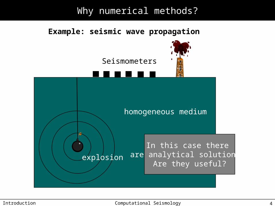
Example: seismic wave propagation
homogeneous medium
Seismometers
explosion
In this case there are analytical solutions?
Are they useful?
Introduction
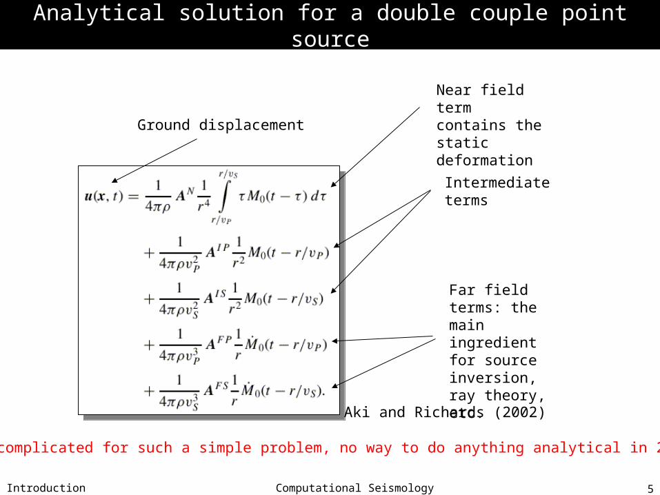
Analytical solution for a double couple point source
Computational Seismology 5
Near field term contains the static deformation
Intermediate terms
Far field terms: the main ingredient for source inversion, ray theory, etc.
Ground displacement
Aki and Richards (2002)
… pretty complicated for such a simple problem, no way to do anything analytical in 2D or 3D!!!!
Introduction
Why numerical methods?
Computational Seismology 6
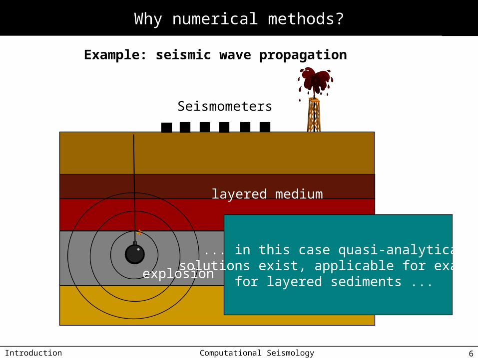
Example: seismic wave propagation
layered medium
Seismometers
explosion
... in this case quasi-analytical solutions exist, applicable for example
for layered sediments ...
Introduction
Why numerical methods?
Computational Seismology 7
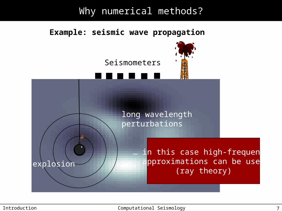
Example: seismic wave propagation
long wavelength perturbations
Seismometers
explosion
… in this case high-frequency approximations can be used
(ray theory)
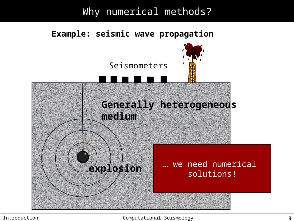
Introduction Computational Seismology 8
Example: seismic wave propagation
Generally heterogeneousmedium
Seismometers
explosion … we need numerical solutions!
Why numerical methods?
Introduction
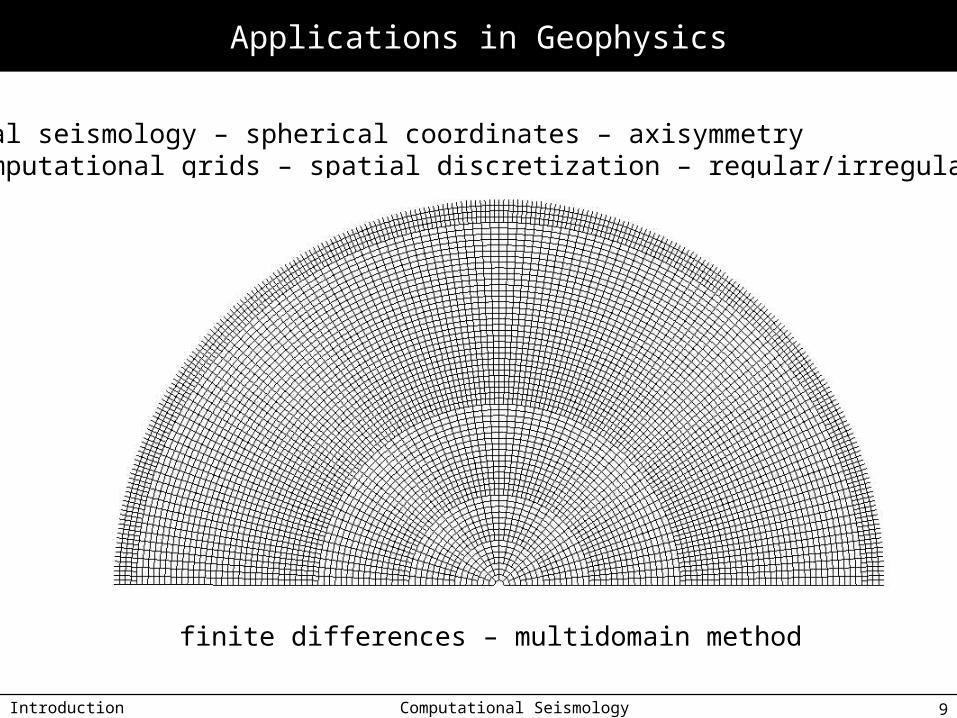
Applications in Geophysics
Computational Seismology 9
global seismology – spherical coordinates – axisymmetry- computational grids – spatial discretization – regular/irregular grids
finite differences – multidomain method

Introduction
Global wave propagation
Computational Seismology 10
PcPpP
P
PKP
Inner core
Outer core
Mantle
global seismology – spherical coordinates - axisymmetry
finite differences – multidomain method

Introduction
Global wave propagation
Computational Seismology 11
finite differences – multidomain method
global seismology – spherical coordinates - axisymmetry
Introduction
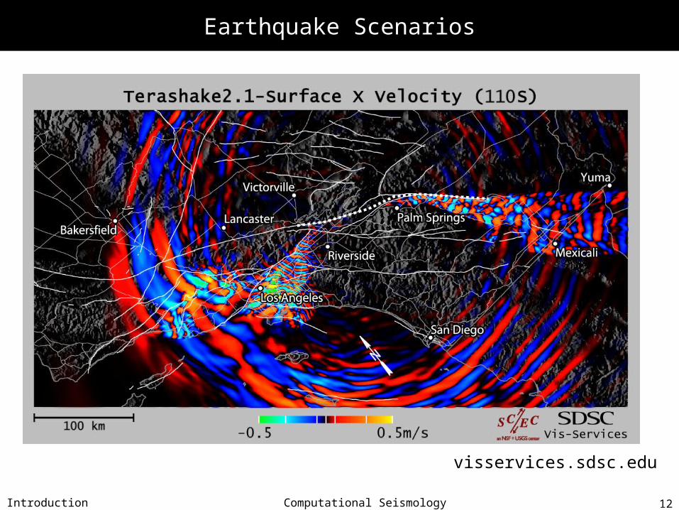
Earthquake Scenarios
Computational Seismology 12
visservices.sdsc.edu
Introduction
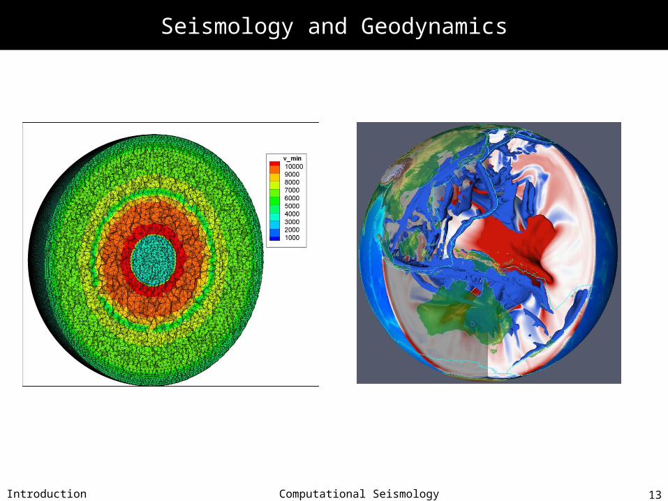
Seismology and Geodynamics
Computational Seismology 13
Introduction
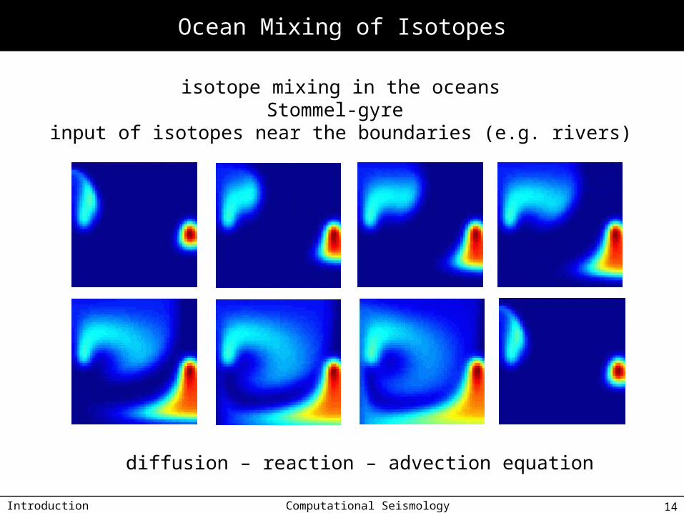
Ocean Mixing of Isotopes
Computational Seismology 14
isotope mixing in the oceansStommel-gyre
input of isotopes near the boundaries (e.g. rivers)
diffusion – reaction – advection equation
Introduction
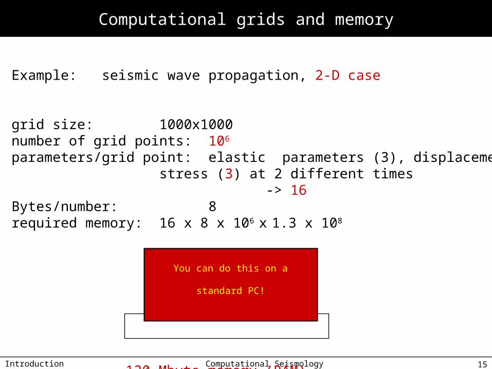
Computational grids and memory
Computational Seismology 15
Example: seismic wave propagation, 2-D case
grid size: 1000x1000number of grid points: 106
parameters/grid point: elastic parameters (3), displacement (2), stress (3) at 2 different times
-> 16 Bytes/number: 8required memory: 16 x 8 x 106 x 1.3 x 108
130 Mbyte memory (RAM)
You can do this on a standard PC!
Introduction
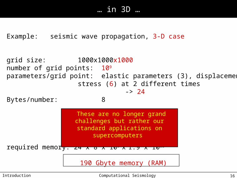
… in 3D …
Computational Seismology 16
Example: seismic wave propagation, 3-D case
grid size: 1000x1000x1000number of grid points: 109
parameters/grid point: elastic parameters (3), displacement (3), stress (6) at 2 different times
-> 24 Bytes/number: 8
required memory: 24 x 8 x 109 x 1.9 x 1011
190 Gbyte memory (RAM)
These are no longer grand challenges but rather our standard applications on
supercomputers
Introduction
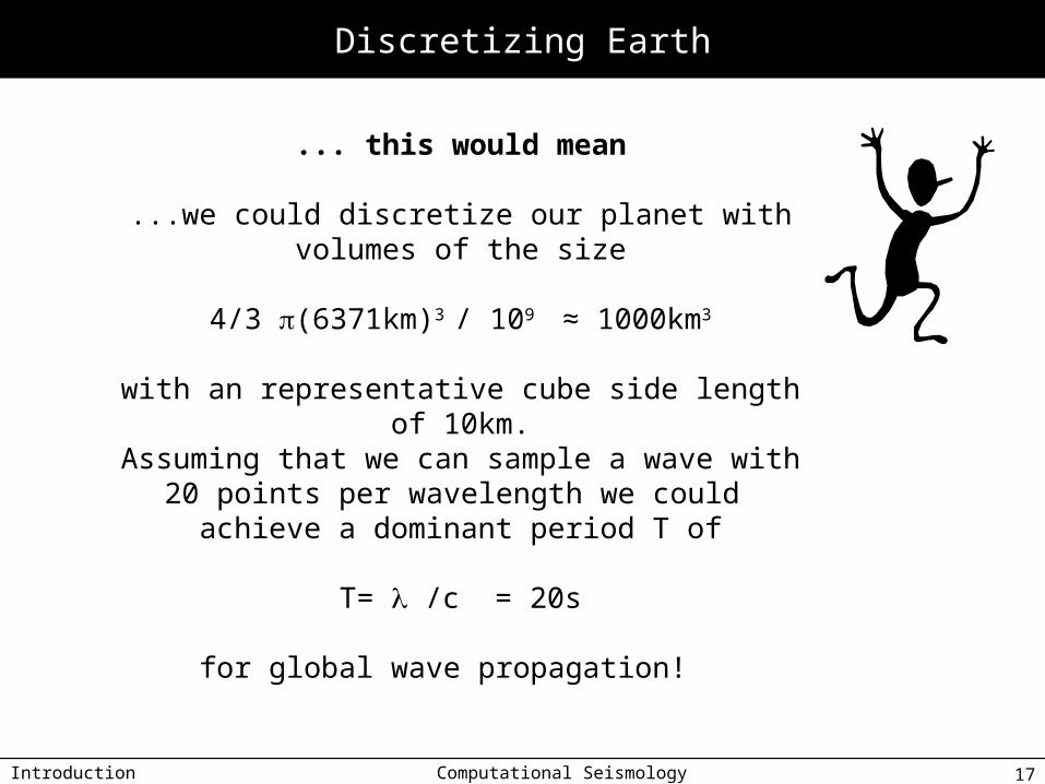
Discretizing Earth
Computational Seismology 17
... this would mean
...we could discretize our planet with volumes of the size
4/3 (6371km)3 / 109 ≈ 1000km3
with an representative cube side length of 10km.Assuming that we can sample a wave with 20 points
per wavelength we could achieve a dominant period T of
T= /c = 20s
for global wave propagation!
Introduction
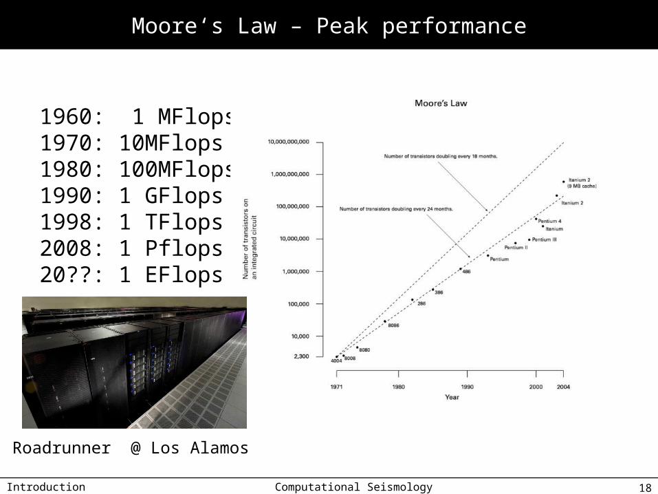
Moore‘s Law – Peak performance
Computational Seismology 18
1960: 1 MFlops1970: 10MFlops1980: 100MFlops1990: 1 GFlops1998: 1 TFlops2008: 1 Pflops20??: 1 EFlops
Roadrunner @ Los Alamos
Introduction
Parallel Computations
Computational Seismology 19
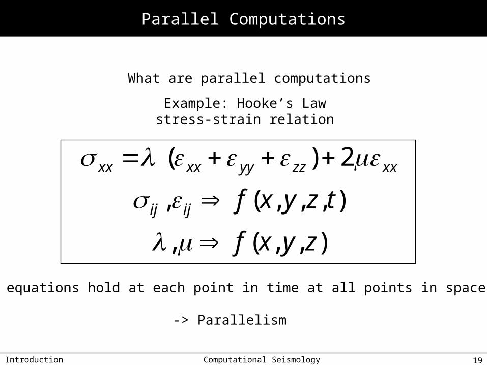
What are parallel computations
Example: Hooke’s Lawstress-strain relation
),,(,
),,,(,
2)(
zyxf
tzyxfijij
xxzzyyxxxx
These equations hold at each point in time at all points in space
-> Parallelism
Introduction
Loops
Computational Seismology 20
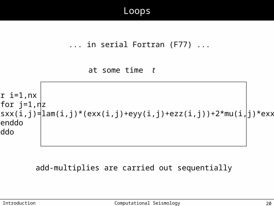
... in serial Fortran (F77) ...
for i=1,nx for j=1,nz sxx(i,j)=lam(i,j)*(exx(i,j)+eyy(i,j)+ezz(i,j))+2*mu(i,j)*exx(i,j) enddoenddo
add-multiplies are carried out sequentially
at some time t
Introduction
Programming Models
Computational Seismology 21
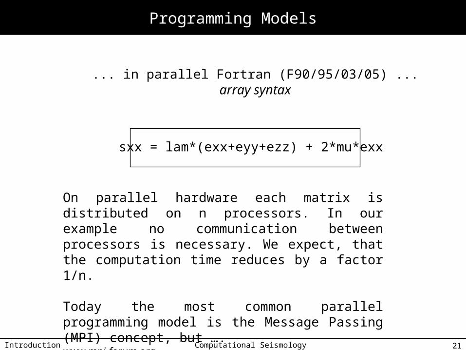
... in parallel Fortran (F90/95/03/05) ...array syntax
sxx = lam*(exx+eyy+ezz) + 2*mu*exx
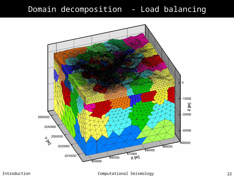
On parallel hardware each matrix is distributed on n processors. In our example no communication between processors is necessary. We expect, that the computation time reduces by a factor 1/n.
Today the most common parallel programming model is the Message Passing (MPI) concept, but ….www.mpi-forum.org
Introduction
Domain decomposition - Load balancing
Computational Seismology 22
Introduction
Macro- vs. microscopic description
Computational Seismology 23
Macroscopic description:
The universe is considered a continuum. Physical processes are described using partial differential equations. The described quantities (e.g. density, pressure, temperature) are really averaged over a certain volume.
Microscopic description:
If we decrease the scale length or we deal with strong discontinous phenomena we arrive at the discrete world(molecules, minerals, atoms, gas particles). If we are interestedin phenomena at this scale we have to take into account the detailsof the interaction between particles.
Introduction
Macro- vs. microscopic description
Computational Seismology 24
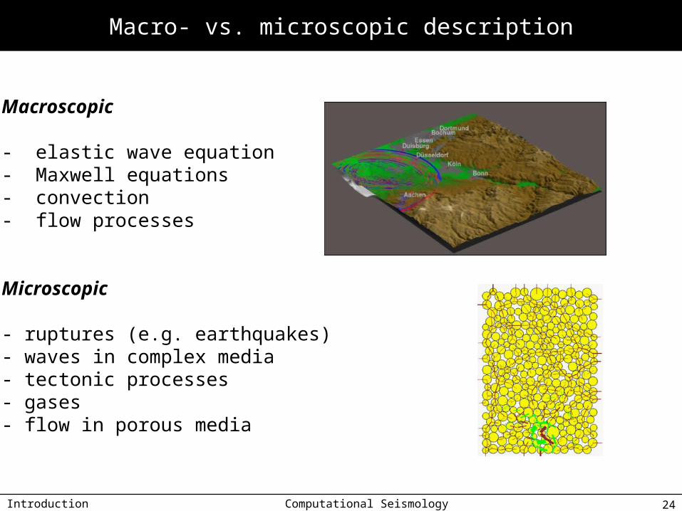
Macroscopic
- elastic wave equation- Maxwell equations - convection - flow processes
Microscopic
- ruptures (e.g. earthquakes)- waves in complex media- tectonic processes- gases- flow in porous media

Introduction
Partial Differential Equations in Geophysics
Computational Seismology 25
0ρ)(vρ jjt
conservation equations
mass
iijjijjt f)vv(ρρ)(v σ momentum
iii gsf gravitation (g) und sources (s)
Introduction
Partial Differential Equations in Geophysics
Computational Seismology 26
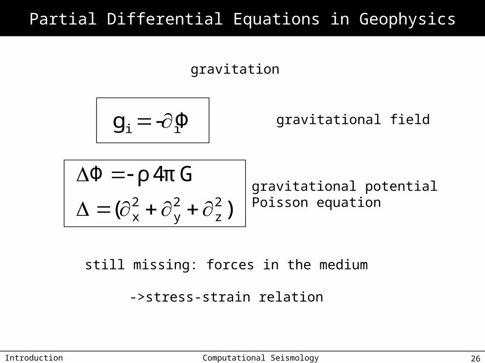
Φ-g ii
gravitation
)
πρΦ2z
2y
2x(
G4
gravitational potentialPoisson equation
gravitational field
still missing: forces in the medium
->stress-strain relation
Introduction
Partial Differential Equations in Geophysics
Computational Seismology 27
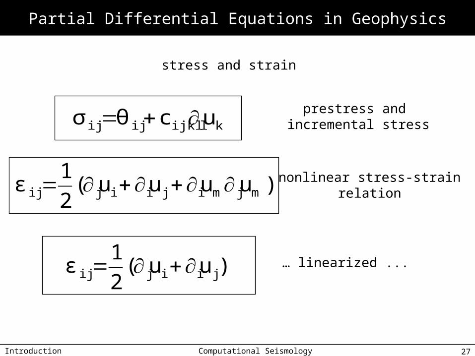
klijklijij ucθσ
stress and strain
)uuuu(2
1ε mjmijiijij nonlinear stress-strain
relation
prestress and incremental stress
)uu(2
1ε jiijij … linearized ...
Introduction
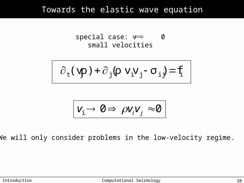
Towards the elastic wave equation
Computational Seismology 28
special case: v 0small velocities
iijjijjt f)vv(ρρ)(v σ
00 jivvv i
We will only consider problems in the low-velocity regime.
Introduction
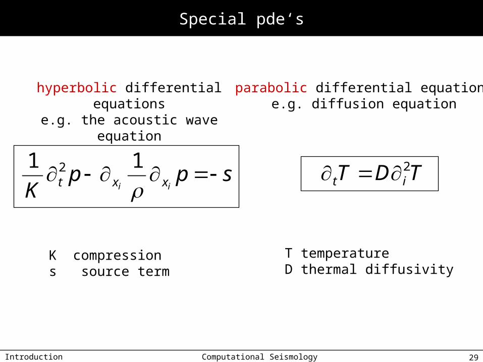
Special pde‘s
Computational Seismology 29
hyperbolic differential equationse.g. the acoustic wave equation
sppK ii xxt
11 2
K compressions source term
parabolic differential equationse.g. diffusion equation
TDT it2
T temperatureD thermal diffusivity
Introduction
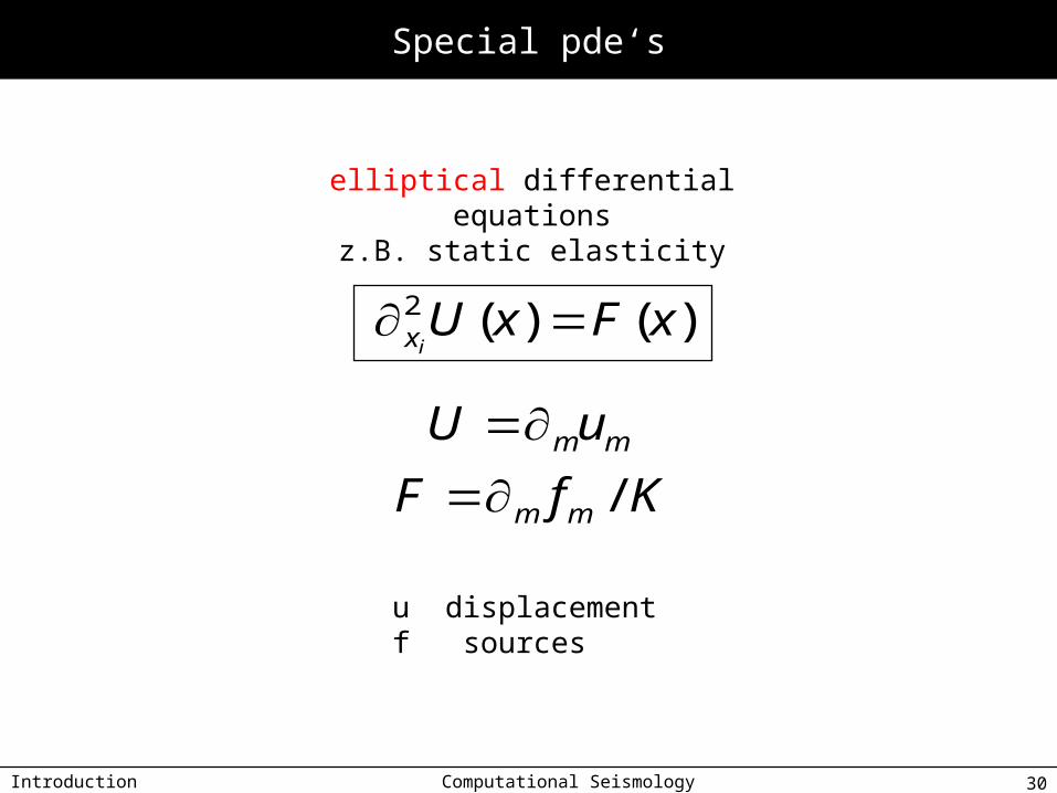
Special pde‘s
Computational Seismology 30
elliptical differential equationsz.B. static elasticity
)()(2 xFxUix
mmuU KfF mm /
u displacementf sources

Introduction
Our Goal
Approximate the wave equation with a discrete scheme that can be solved numerically in a computer
Develop the algorithms for the 1-D wave equation and investigate their behavior
Understand the limitations and pitfalls of numerical solutions to pde‘s Courant criterion Numerical anisotropy Stability Numerical dispersion Benchmarking
Computational Seismology 31
Introduction
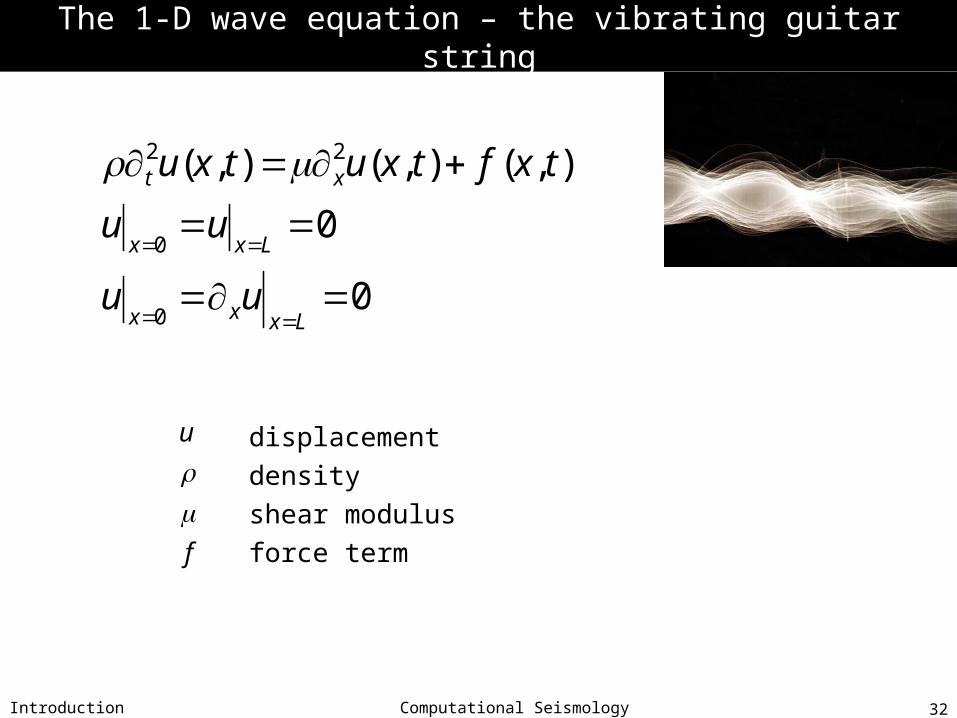
The 1-D wave equation – the vibrating guitar string
Computational Seismology 32
0
0
),(),(),(
0
0
22
Lxxx
Lxx
xt
uu
uu
txftxutxu
displacement
density
shear modulus
force termf
u

Introduction
Summary
Computational Seismology 33
Numerical method play an increasingly important role in all domains ofgeophysics.
The development of hardware architecture allows an efficient calculationof large scale problems through parallelization.
Most of the dynamic processes in geophysics can be described with time-dependent partial differential equations.
The main problem will be to find ways to determine how best to solvethese equations with numerical methods.