Embed Size (px)
Citation preview
Introduction
Chapter 1
Topics
1.2 Classification of Signals: (1.2.1),(1.2.2), (1.2.3), (1.2.4)
1.3 The concept of frequency in continuous-time and discrete-time signals: (1.3.1), (1.3.2)
1.4 A/D and D/A conversion: (1.4.1), (1.4.2)
Examples and Problems
Examples: (1.4.1) , (1.4.2) , (1.4.3), (1.4.4)
Important Problems: 1.2 , 1.5 , 1.7 , 1.9
Practice Problems: 1.3 , 1.8 , 1.15
What is
Digital Signal Processing?
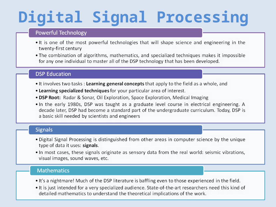
Digital Signal Processing
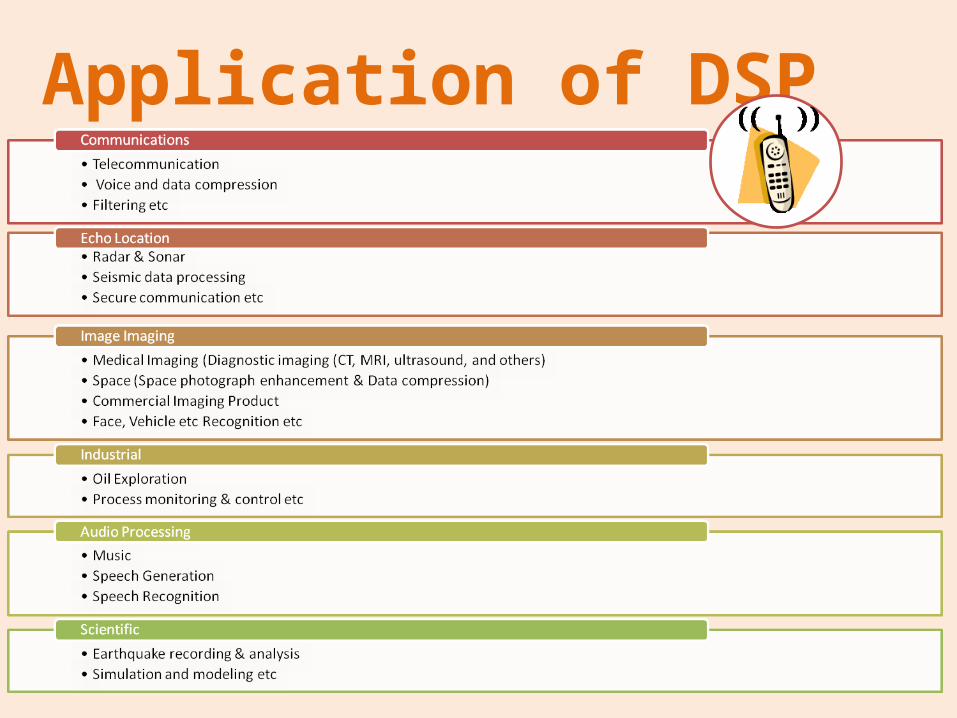
Application of DSP
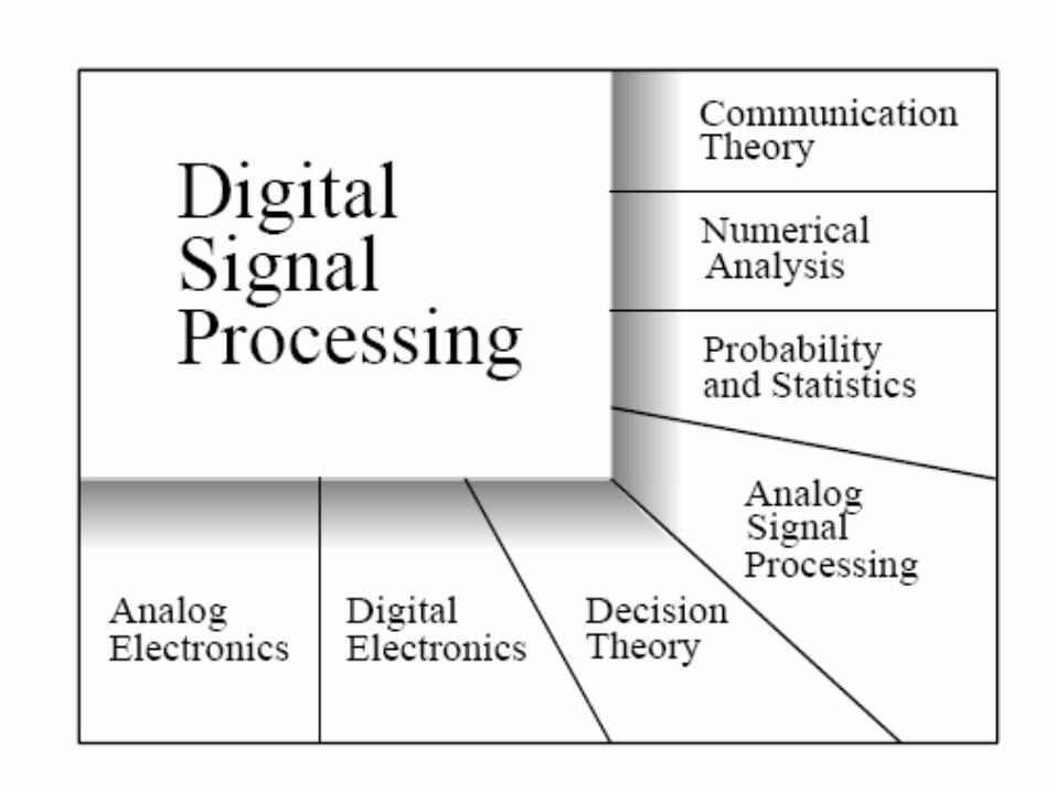
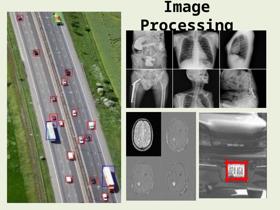
Image Processing
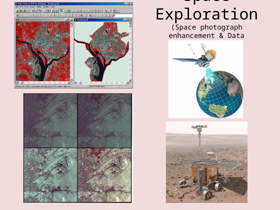
Space Exploration(Space photograph enhancement &
Data compression)
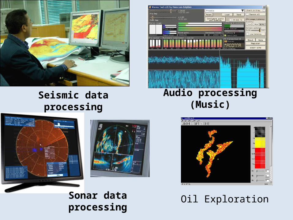
Seismic data processing
Sonar data processing
Audio processing (Music)
Oil Exploration

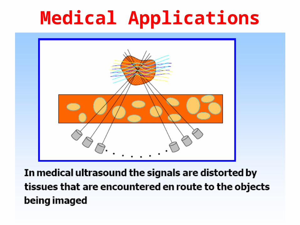
Medical Applications
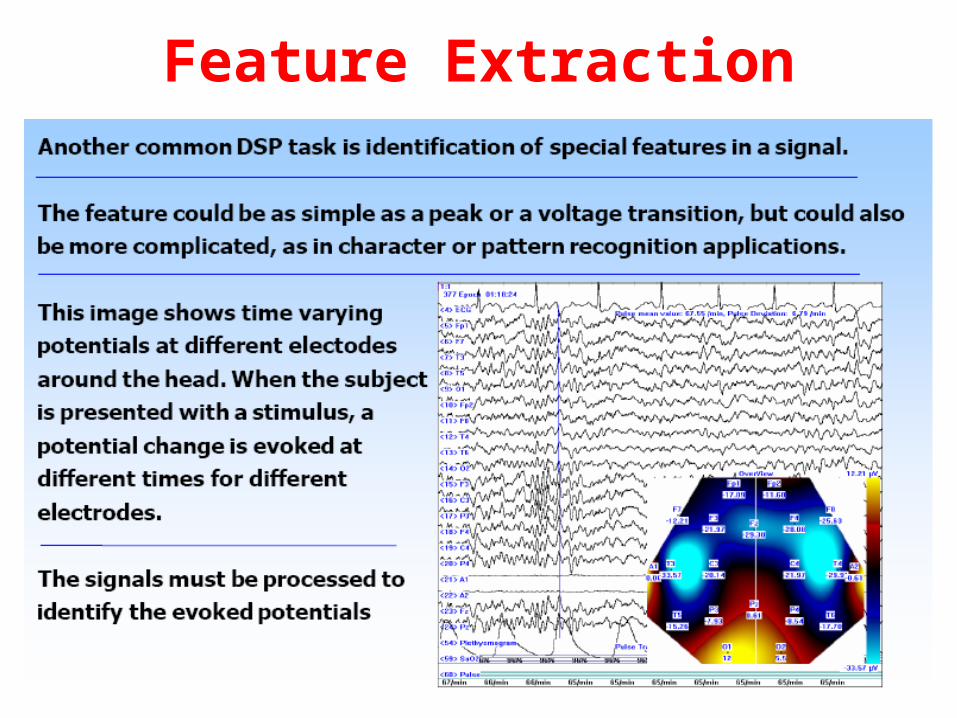
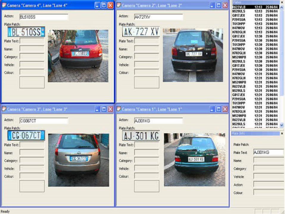
Feature Extraction
Signal• Any entity that varies with one or more independent
entity such that all these entities should have a physical meaning.
• (e.g. time, frequency, space, etc.) and both has a physical meaning and has the ability to convey information.
• Examples1. Electrical signals (Radio communications signals, audio and video etc).
2. Mechanical signals (vibrations in a structure, earthquakes).
3. Biomedical signals (EEG, lung and heart monitoring, X-ray etc).
• The most convenient mathematical representation of a signal is via the concept of a function. S(t) = at
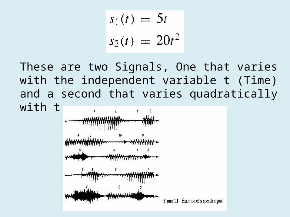
These are two Signals, One that varies with the independent variable t (Time) and a second that varies quadratically with t
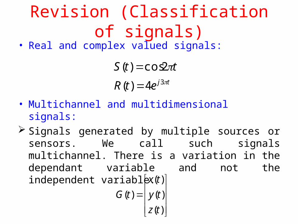
Revision (Classification of signals)• Real and complex valued signals:
• Multichannel and multidimensional signals: Signals generated by multiple sources or sensors.
We call such signals multichannel. There is a variation in the dependant variable and not the independent variable.
tjetR
ttS
34)(
2cos)(
)(
)(
)(
)(
tz
ty
tx
tG
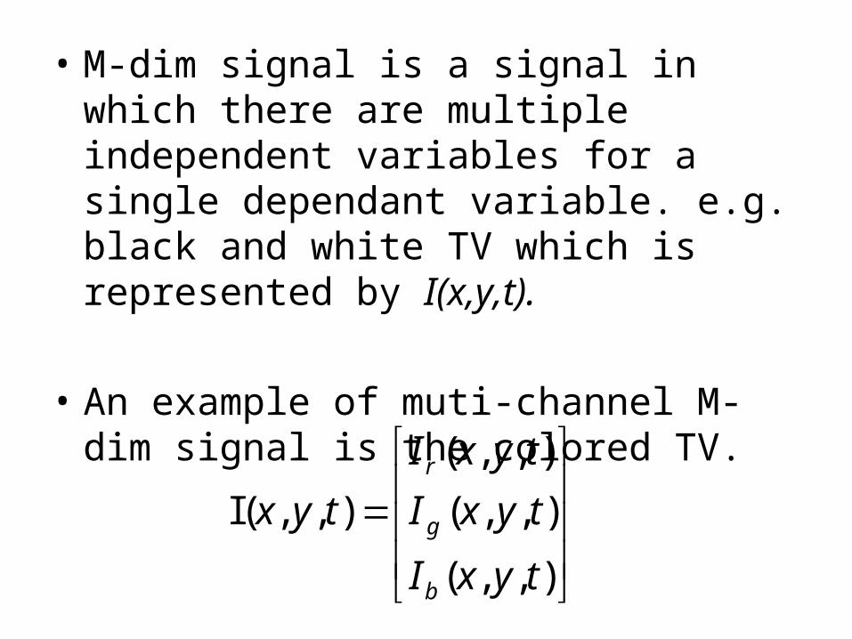
• M-dim signal is a signal in which there are multiple independent variables for a single dependant variable. e.g. black and white TV which is represented by I(x,y,t).
• An example of muti-channel M-dim signal is the colored TV.
),,(
),,(
),,(
),,(I
tyxI
tyxI
tyxI
tyx
b
g
r
19
Classification of signals contd.
• Deterministic signals: are those signals which we can construct using a mathematical relation, table lookup and by other means.
• Random signals: those signals which have some level of uncertainty. We can estimate these signals
by statistical and probabilistic means.
20
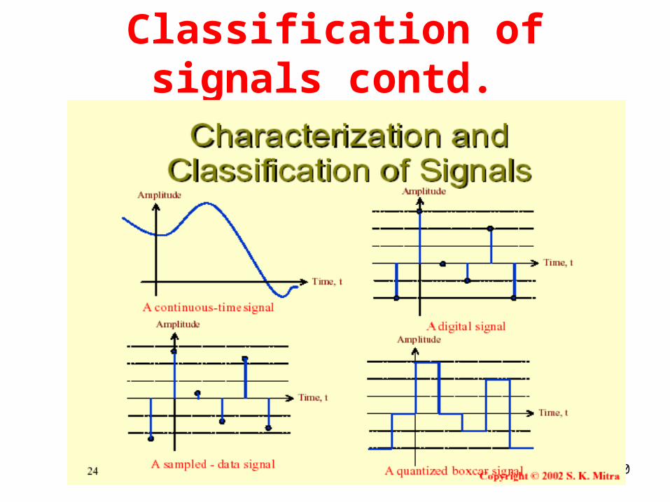
Classification of signals contd.
21
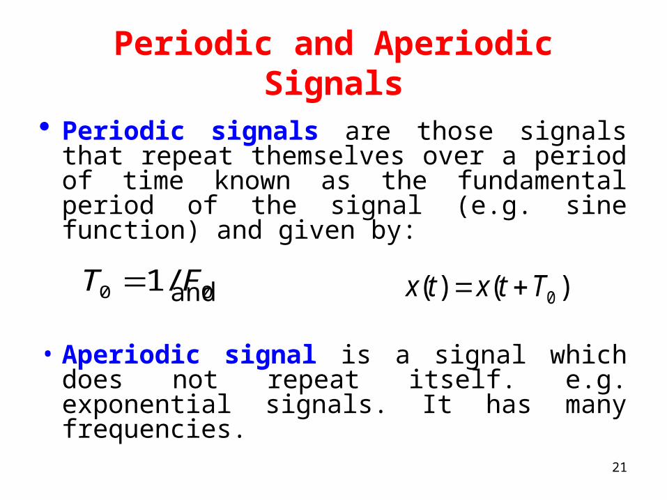
Periodic and Aperiodic Signals
Periodic signals are those signals that repeat themselves over a period of time known as the fundamental period of the signal (e.g. sine function) and given by:
and
• Aperiodic signal is a signal which does not repeat itself. e.g. exponential signals. It has many frequencies.
00 /1 FT )()( 0Ttxtx
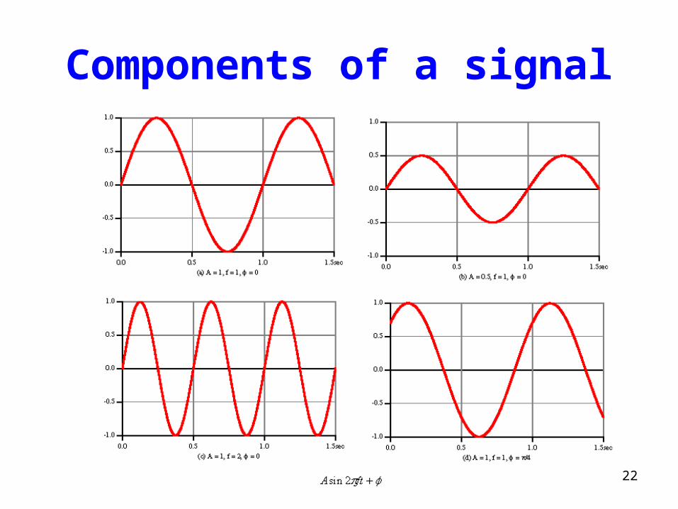
22
Components of a signal
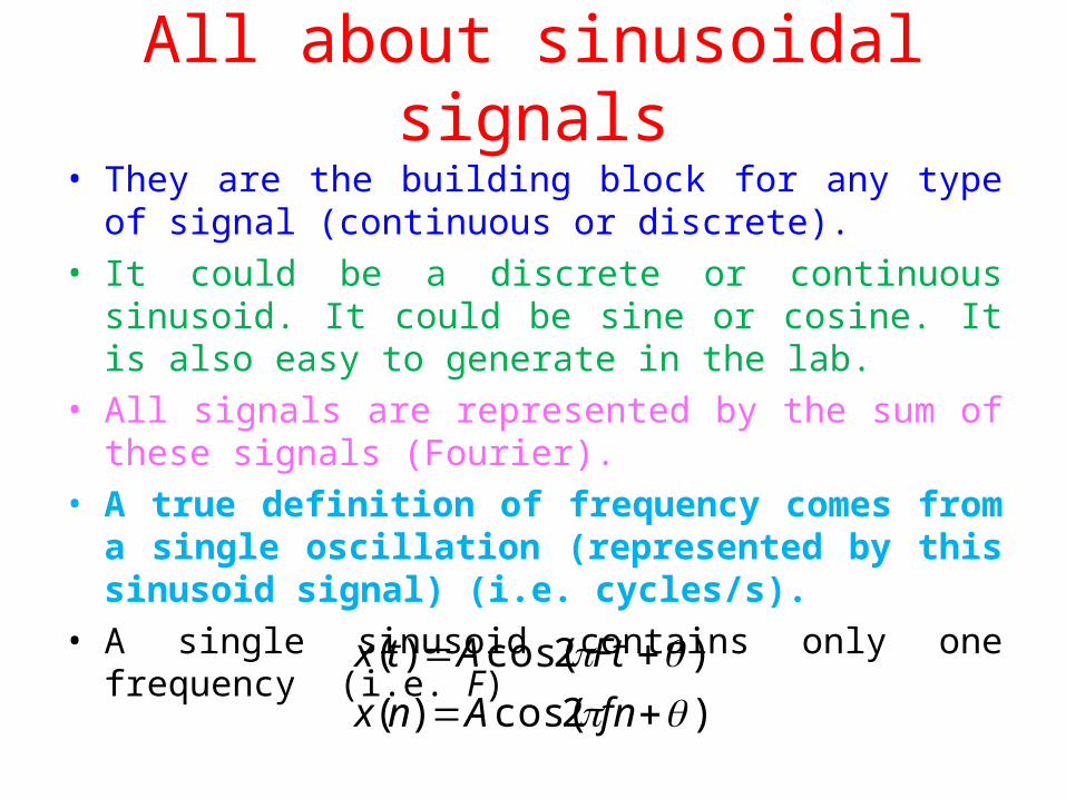
All about sinusoidal signals• They are the building block for any type of signal
(continuous or discrete).• It could be a discrete or continuous sinusoid. It could be
sine or cosine. It is also easy to generate in the lab.• All signals are represented by the sum of these signals
(Fourier).• A true definition of frequency comes from a single
oscillation (represented by this sinusoid signal) (i.e. cycles/s).
• A single sinusoid contains only one frequency (i.e. F)
)2cos()(
)2cos()(
fnAnx
FtAtx
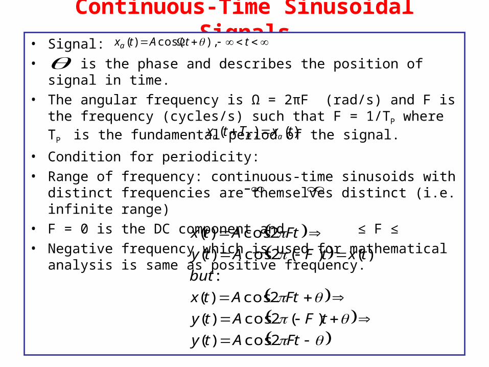
Continuous-Time Sinusoidal Signals• Signal:• is the phase and describes the position of signal in time.• The angular frequency is Ω = 2πF (rad/s) and F is the frequency
(cycles/s) such that F = 1/TP where TP is the fundamental period of the signal.
• Condition for periodicity: • Range of frequency: continuous-time sinusoids with distinct
frequencies are themselves distinct (i.e. infinite range)• F = 0 is the DC component and ≤ F ≤ • Negative frequency which is used for mathematical analysis is same
as positive frequency.
ttAtxa ),cos()(
)()( txTtx aPa
FtAty
tFAty
FtAtx
but
txtFAty
FtAtx
2cos)(
)(2cos)(
2cos)(
:
)()(2cos)(
2cos)(
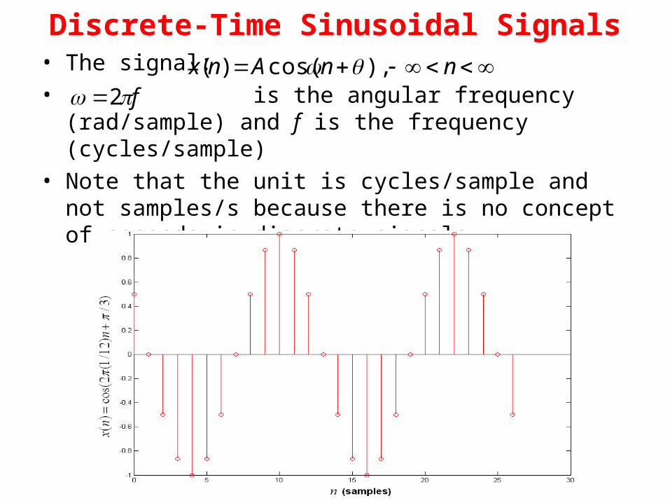
Discrete-Time Sinusoidal Signals• The signal:• is the angular frequency (rad/sample) and f is
the frequency (cycles/sample) • Note that the unit is cycles/sample and not samples/s
because there is no concept of seconds in discrete signals.
nnAnx ),cos()( f 2
Discrete-Time Sinusoidal Signals contd.
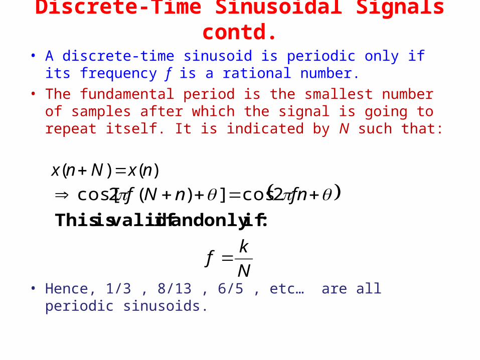
• A discrete-time sinusoid is periodic only if its frequency f is a rational number.
• The fundamental period is the smallest number of samples after which the signal is going to repeat itself. It is indicated by N such that:
• Hence, 1/3 , 8/13 , 6/5 , etc… are all periodic sinusoids.
)()( nxNnx
:if only and if valid is This
fnnNf 2cos])(2cos[
N
kf
Important Things to Note
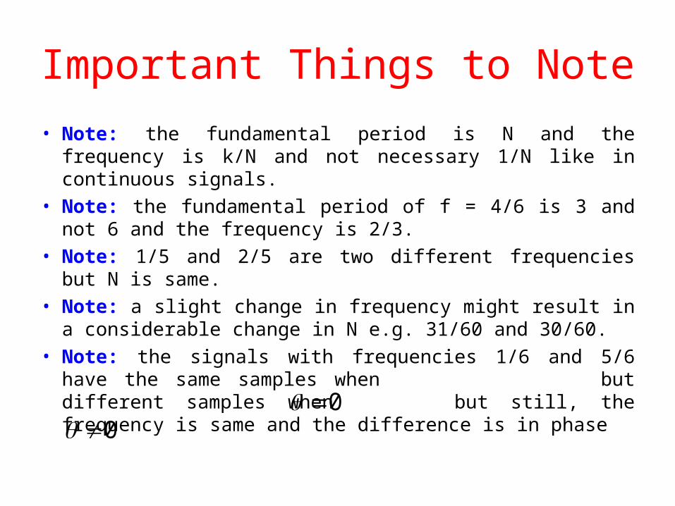
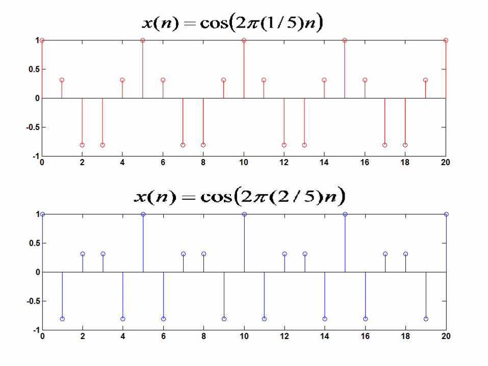
• Note: the fundamental period is N and the frequency is k/N and not necessary 1/N like in continuous signals.
• Note: the fundamental period of f = 4/6 is 3 and not 6 and the frequency is 2/3.
• Note: 1/5 and 2/5 are two different frequencies but N is same.
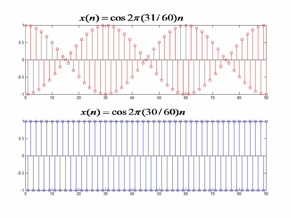
• Note: a slight change in frequency might result in a considerable change in N e.g. 31/60 and 30/60.
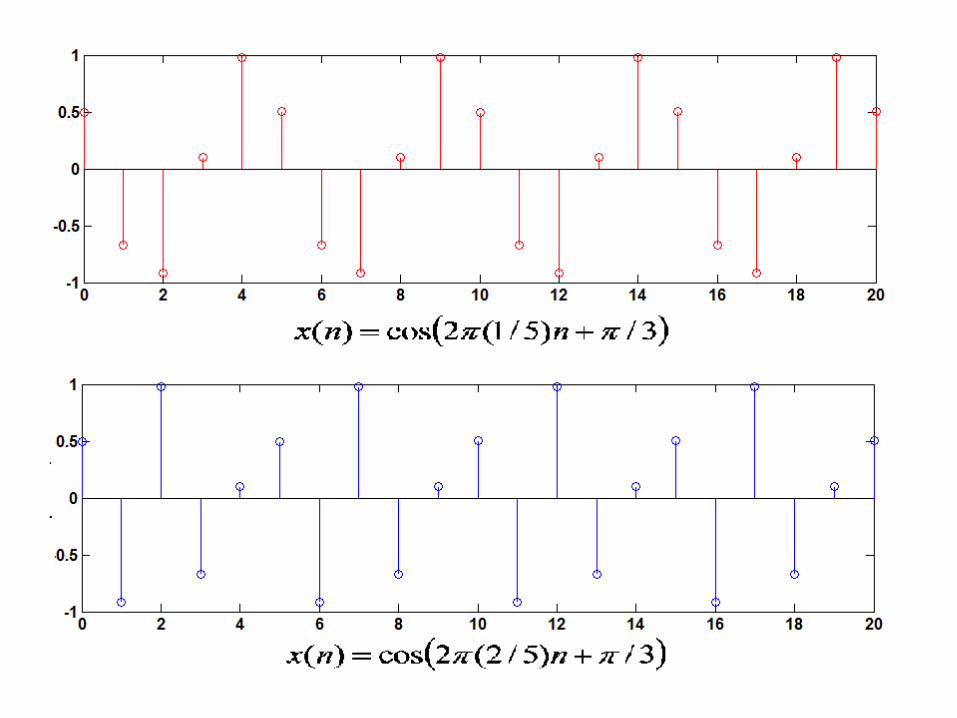
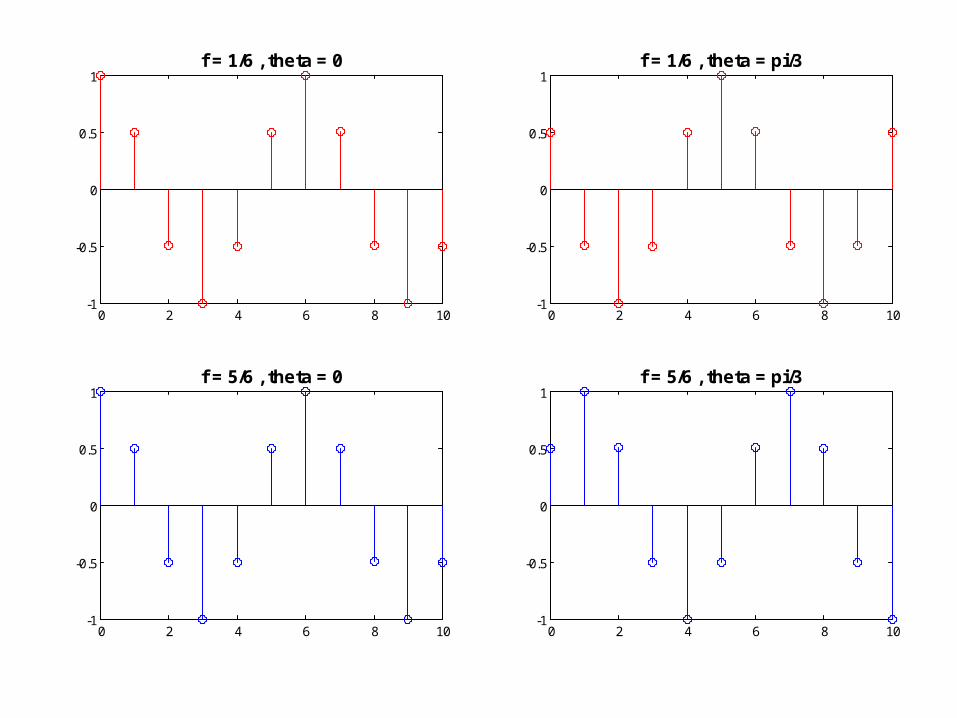
• Note: the signals with frequencies 1/6 and 5/6 have the same samples when but different samples when
but still, the frequency is same and the difference is in phase
00
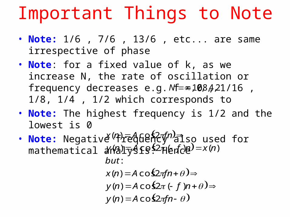
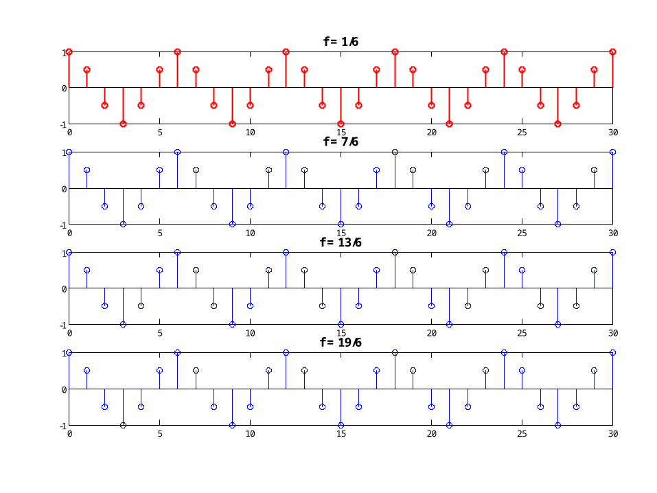
Important Things to Note• Note: 1/6 , 7/6 , 13/6 , etc... are same irrespective of
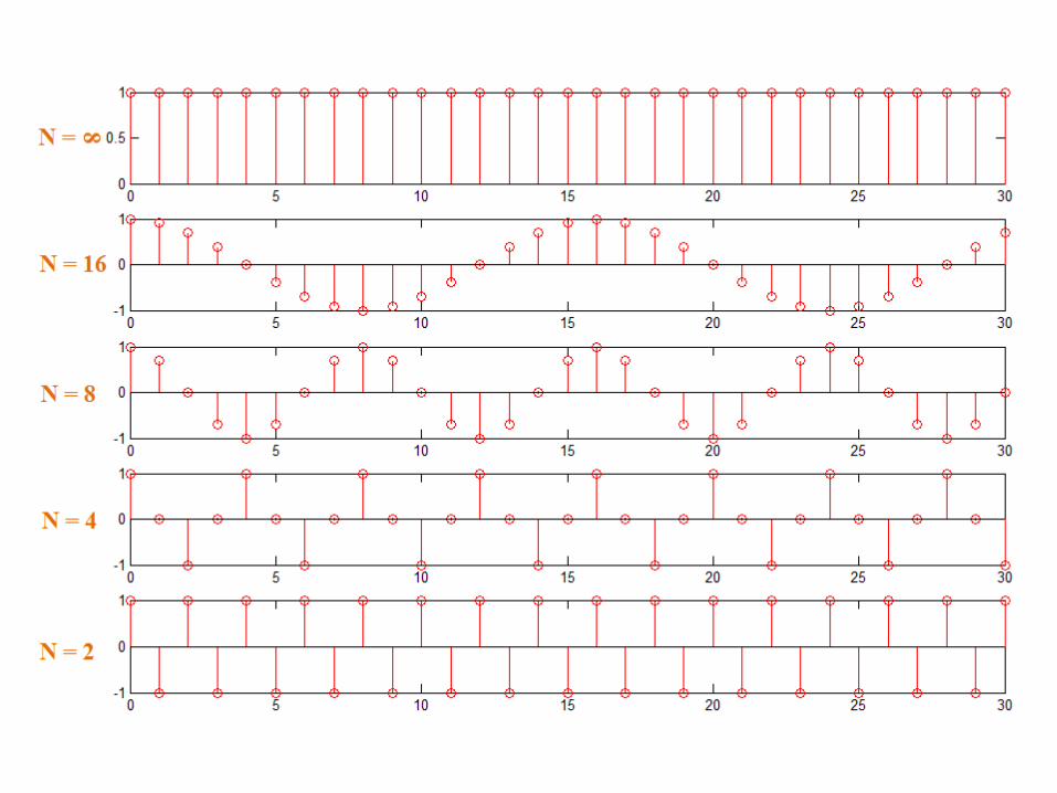
phase• Note: for a fixed value of k, as we increase N, the rate of
oscillation or frequency decreases e.g. f = 0 , 1/16 , 1/8, 1/4 , 1/2 which corresponds to
• Note: The highest frequency is 1/2 and the lowest is 0• Note: Negative frequency also used for mathematical
analysis. Hence
2,4,8,16,N
fnAny
nfAny
fnAnx
but
nxnfAny
fnAnx
2cos)(
)(2cos)(
2cos)(
:
)()(2cos)(
2cos)(
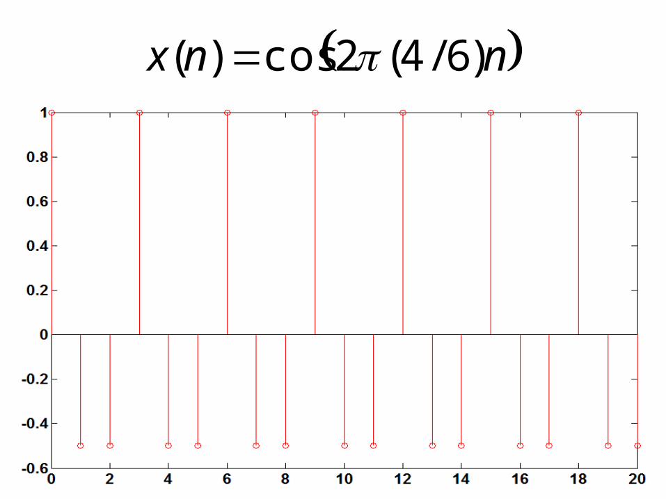
nnx )6/4(2cos)(
0 2 4 6 8 10-1
-0.5
0
0.5
1f = 1/6 , theta = 0
0 2 4 6 8 10-1
-0.5
0
0.5
1f = 5/6 , theta = 0
0 2 4 6 8 10-1
-0.5
0
0.5
1f = 1/6 , theta = pi/3
0 2 4 6 8 10-1
-0.5
0
0.5
1f = 5/6 , theta = pi/3
0 5 10 15 20 25 30-1
0
1f = 1/6
0 5 10 15 20 25 30-1
0
1f = 7/6
0 5 10 15 20 25 30-1
0
1f = 13/6
0 5 10 15 20 25 30-1
0
1f = 19/6
0 5 10 15 20 25 30-1
-0.5
0
0.5
1f = 3/10 , theta = pi/3
0 5 10 15 20 25 30-1
-0.5
0
0.5
1f = -3/10 , theta = pi/3
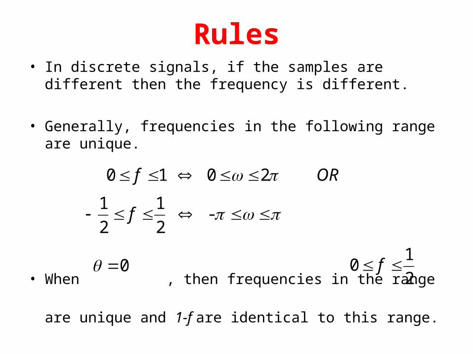
Rules• In discrete signals, if the samples are different then the
frequency is different.
• Generally, frequencies in the following range are unique.
• When , then frequencies in the range
are unique and 1-f are identical to this range.
ORf 20 10
- 2
1
2
1f
0 2
10 f
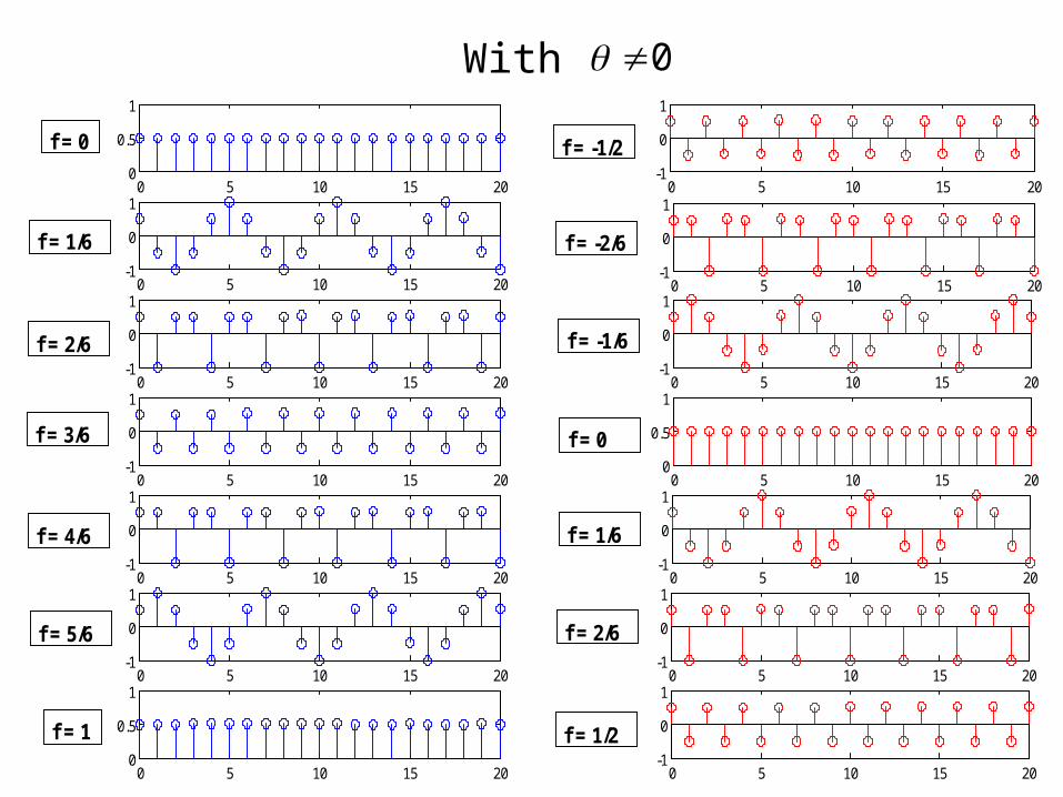
With
0 5 10 15 200
0.5
1
0 5 10 15 20-1
0
1
0 5 10 15 20-1
0
1
0 5 10 15 20-1
0
1
0 5 10 15 20-1
0
1
0 5 10 15 20-1
0
1
0 5 10 15 20-1
0
1
0 5 10 15 200
0.5
1
0 5 10 15 20-1
0
1
0 5 10 15 20-1
0
1
0 5 10 15 20-1
0
1
0 5 10 15 20-1
0
1
0 5 10 15 200
0.5
1
0 5 10 15 20-1
0
1
f = 0
f = 1/6
f = 1
f = 2/6
f = 3/6
f = 4/6
f = 5/6
f = -1/2
f = -2/6
f = -1/6
f = 0
f = 1/6
f = 2/6
f = 1/2
0

With
0 5 10 15 200
0.5
1
0 5 10 15 20-1
0
1
0 5 10 15 20-1
0
1
0 5 10 15 20-1
0
1
0 5 10 15 20-1
0
1
0 5 10 15 20-1
0
1
0 5 10 15 20-1
0
1
0 5 10 15 200
0.5
1
0 5 10 15 20-1
0
1
0 5 10 15 20-1
0
1
0 5 10 15 20-1
0
1
0 5 10 15 20-1
0
1
0 5 10 15 200
0.5
1
0 5 10 15 20-1
0
1
f = 0
f = 1/6
f = 2/6
f = 3/6
f = 4/6
f = 5/6
f = 1
f = -1/2
f = -2/6
f = -1/6
f = 0
f = 1/6
f = 2/6
f = 1/2
0
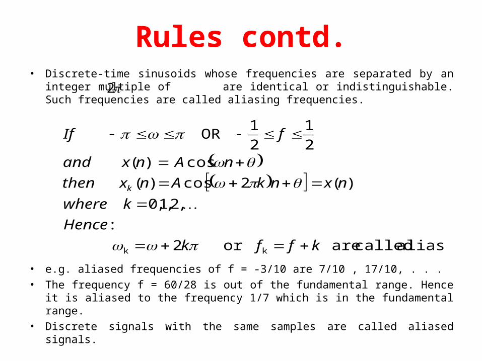
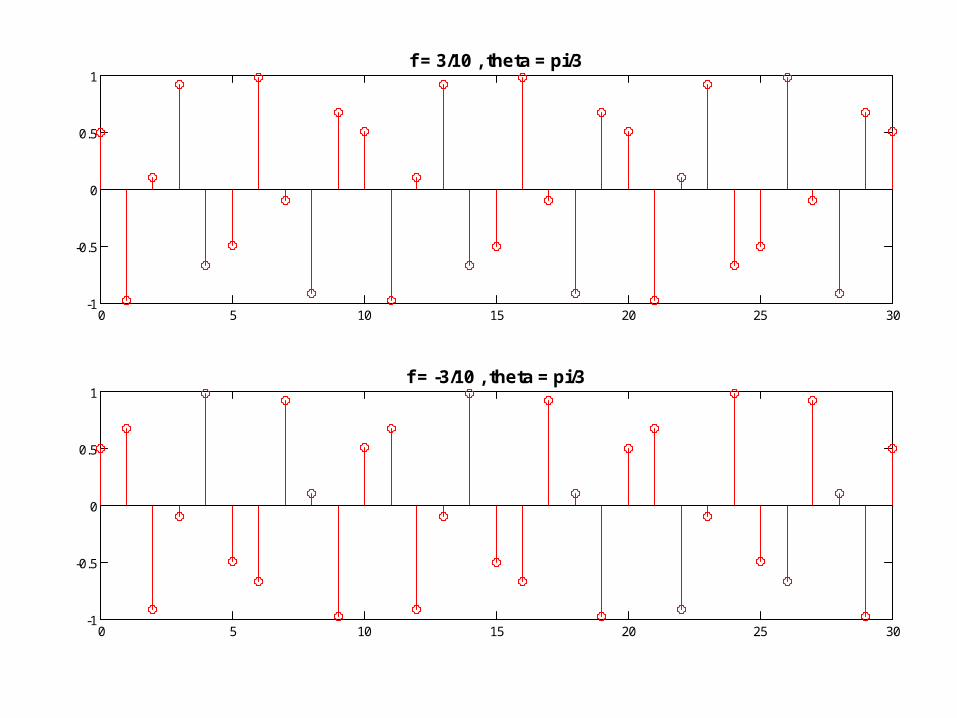
Rules contd.• Discrete-time sinusoids whose frequencies are separated by an integer
multiple of are identical or indistinguishable. Such frequencies are called aliasing frequencies.
• e.g. aliased frequencies of f = -3/10 are 7/10 , 17/10, . . .
• The frequency f = 60/28 is out of the fundamental range. Hence it is aliased to the frequency 1/7 which is in the fundamental range.
• Discrete signals with the same samples are called aliased signals.
2
aliased called are or 2
:
,2,1,0
)(2cos)(
cos )( 2
1
2
1 OR
kk kffk
Hence
kwhere
nxnkAnxthen
nAnxand
fIf
k
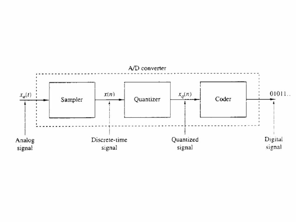
Analog to Digital Convertor• The performance of A/D converter depends on two processes:
sampling and quantization.
• The digital signal is an approximation of the analog signal. It means that A/D conversion results in information loss.
• The process of D/A conversion is done using different interpolation methods.
• Quantization results in loss of information. This could be controlled using a better quality quantizer.
• Sampling does not result in information loss if and only if our signal is band limited. But such sampling is only theoretical.
• Accuracy of the A/D depends on the quality of quantizer and
sampling rate. Higher the accuracy, more will be the cost.
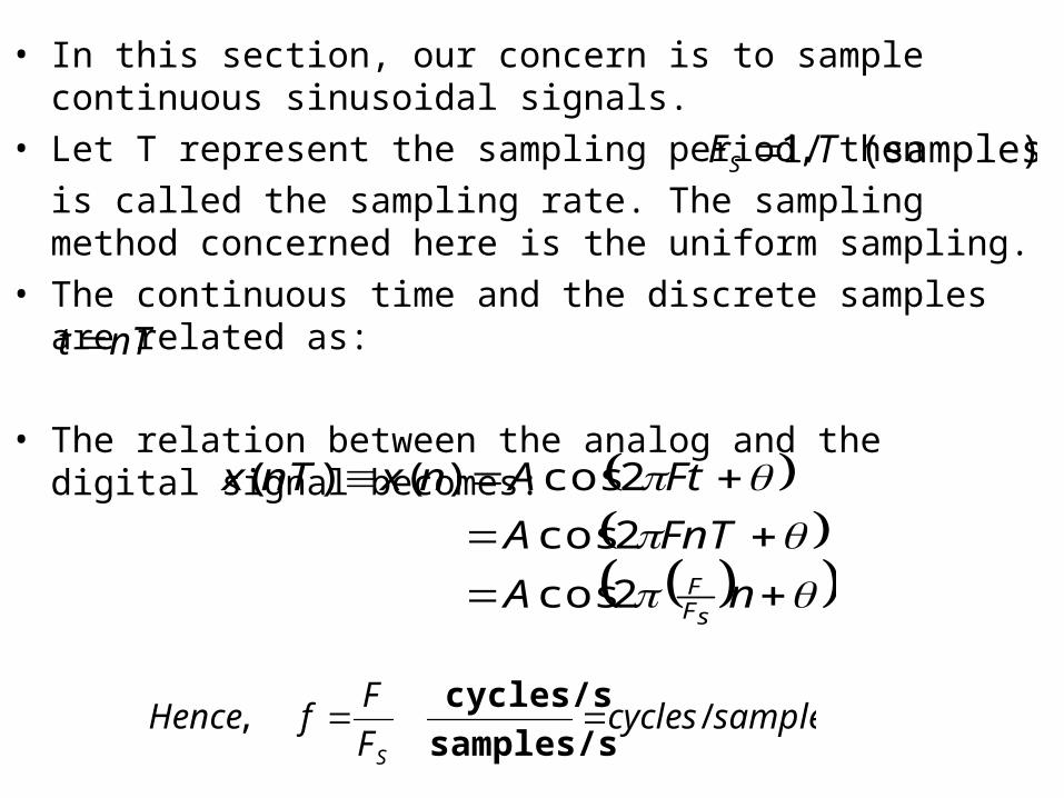
• In this section, our concern is to sample continuous sinusoidal signals.
• Let T represent the sampling period, then
is called the sampling rate. The sampling method concerned here is the uniform sampling.
• The continuous time and the discrete samples are related as:
• The relation between the analog and the digital signal
becomes:
)(samples/s /1 TFS
nTt
nA
FnTA
FtAnxnTx
sFF2cos
2cos
2cos)()(
samplecyclesF
FfHence
S
/, samples/s
cycles/s
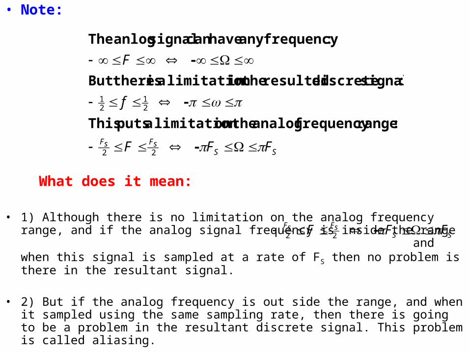
• Note:
What does it mean:
• 1) Although there is no limitation on the analog frequency range, and if the analog signal frequency is inside the range and when this signal is sampled at a rate of FS then no problem is there in the resultant signal.
• 2) But if the analog frequency is out side the range, and when it sampled using the same sampling rate, then there is going to be a problem in the resultant discrete signal. This problem is called aliasing.
SSsFsF FFF
f
F
-
:range frequency analog the on limitation a puts This
-
:signal discrete resulted the in limitation a is thereBut
-
:frequency any have can signal anlog The
22
21
21
SSsFsF FFF - 22
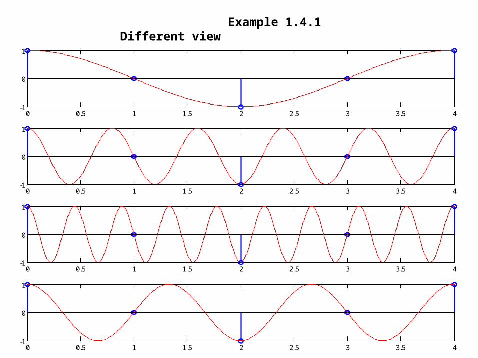
Aliasing
• The folding point: is a positive frequency point after which aliasing occurs when the analog signal is sampled at FS Hz. This frequency equals to the upper limit of the range (i.e. FS/2).
• Aliasing can be explained both in time and frequency domain. In this section, we are going to see the aliasing in time domain.
• Find out yourself the aliasing in frequency domain.
• Example 1.4.1
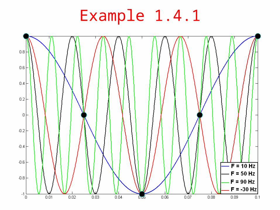
Example 1.4.1
0 0.5 1 1.5 2 2.5 3 3.5 4-1
0
1
0 0.5 1 1.5 2 2.5 3 3.5 4-1
0
1
0 0.5 1 1.5 2 2.5 3 3.5 4-1
0
1
0 0.5 1 1.5 2 2.5 3 3.5 4-1
0
1
Example 1.4.1 Different view
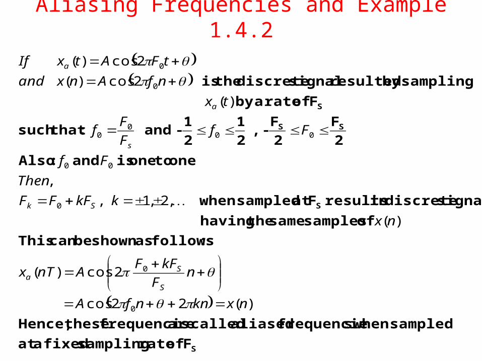
Aliasing Frequencies and Example 1.4.2
S
S
SS
S
F of rate sampling fixed aat
sampled when sfrequencie aliased called are frequencis these Hence,
:follows as shown be can This
of samples same the having
signals discrete in results Fat sampled when
one to one is and :Also
2
F
2
F- ,
2
1
2
1- and :that such
F of rate a by
sampling by resulted signal discrete the is
)(22cos
2cos)(
)(
,2,1,
,
)(
2cos)(
2cos)(
0
0
0
00
000
0
0
0
nxknnfA
nF
kFFAnTx
nx
kkFFF
Then
Ff
FfF
Ff
tx
nfAnxand
tFAtxIf
S
Sa
Sk
s
a
a
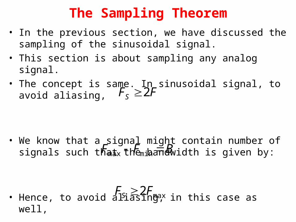
The Sampling Theorem• In the previous section, we have discussed the sampling of
the sinusoidal signal. • This section is about sampling any analog signal.• The concept is same. In sinusoidal signal, to avoid aliasing,
• We know that a signal might contain number of signals such that the bandwidth is given by:
• Hence, to avoid aliasing, in this case as well,
FFS 2
BFF minmax
max2FFS
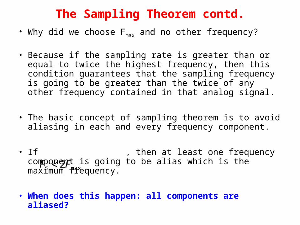
The Sampling Theorem contd.
• Why did we choose Fmax and no other frequency?
• Because if the sampling rate is greater than or equal to twice the highest frequency, then this condition guarantees that the sampling frequency is going to be greater than the twice of any other frequency contained in that analog signal.
• The basic concept of sampling theorem is to avoid aliasing in each and every frequency component.
• If , then at least one frequency component is going to be alias which is the maximum frequency.
• When does this happen: all components are aliased?
max2FFS
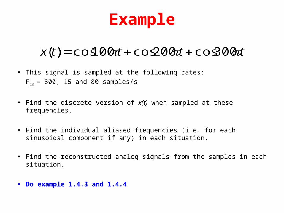
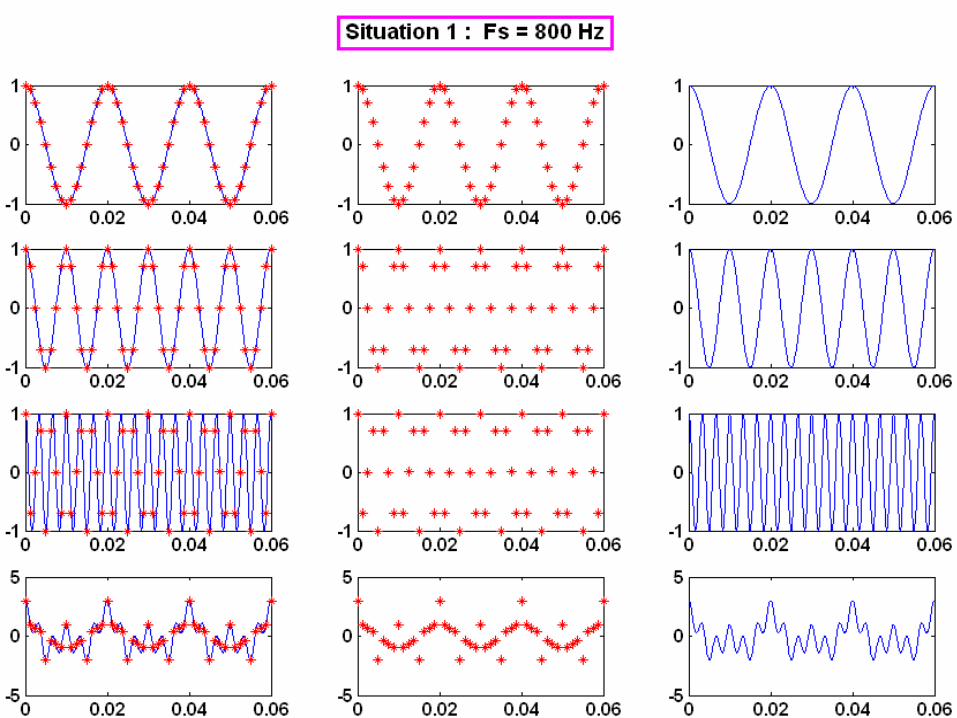
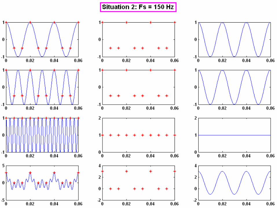
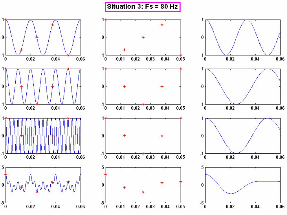
Example
• This signal is sampled at the following rates:
F1s = 800, 15 and 80 samples/s
• Find the discrete version of x(t) when sampled at these frequencies.
• Find the individual aliased frequencies (i.e. for each sinusoidal component if any) in each situation.
• Find the reconstructed analog signals from the samples in each situation.
• Do example 1.4.3 and 1.4.4
ttttx 300cos200cos100cos)(
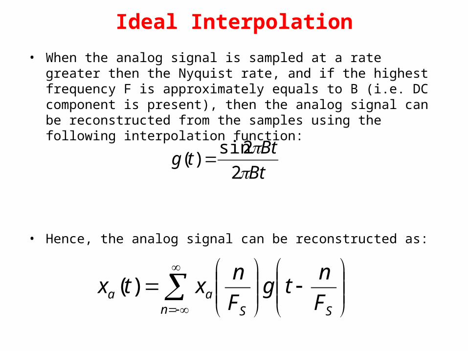
Ideal Interpolation
• When the analog signal is sampled at a rate greater then the Nyquist rate, and if the highest frequency F is approximately equals to B (i.e. DC component is present), then the analog signal can be reconstructed from the samples using the following interpolation function:
• Hence, the analog signal can be reconstructed as:
Bt
Bttg
2
2sin)(
n SSaa F
ntg
F
nxtx )(
Ideal Interpolation contd.
• This reconstruction method is very complicated and impractical.
• It is only used for theoretical purposes.
• It involves a weighted sum of the interpolation function g(t) and its time shifted version g(t-nT) for infinite values of the sample n.
• More practical interpolation techniques are used instead.
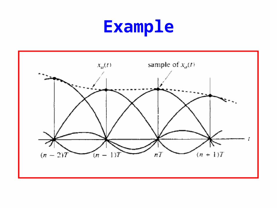
Example
Some sampling issues
• Avoid taking samples at zero crossing points. See example 1.4.3
• One solution is to introduce phase offset but this is not going to totally eliminate this problem
• Optimum solution is oversampling