Teaching philosophy •  Learn it 5-times and you know it

–  Read (& simple question) –  Lecture –  Problem set –  Review/work-problems for Mid-term exam –  Review/re-work for Final exam

•  Hand in homework every Monday (1 per week) –  In-depth problem(s) on previous lectures –  Preview question(s) of coming week’s lecture –  Each problem on a separate sheet of paper! Units! Circle answer!

•  In-class: –  Monday 4-5pm: hand in select problem(s), Work solution to (select) questions –  Monday (±)5-6pm Lecture on new material. –  Tuesday, return homework and review solution, & lecture on new material

125 Hours work-load, 33 lectures, 3-hours independent *per* lecture. Spectroscopy is core to many R&D tasks both Industrial & Academic, it will get you employed, and keep you there (and pay my pension!)

learn it, know it!

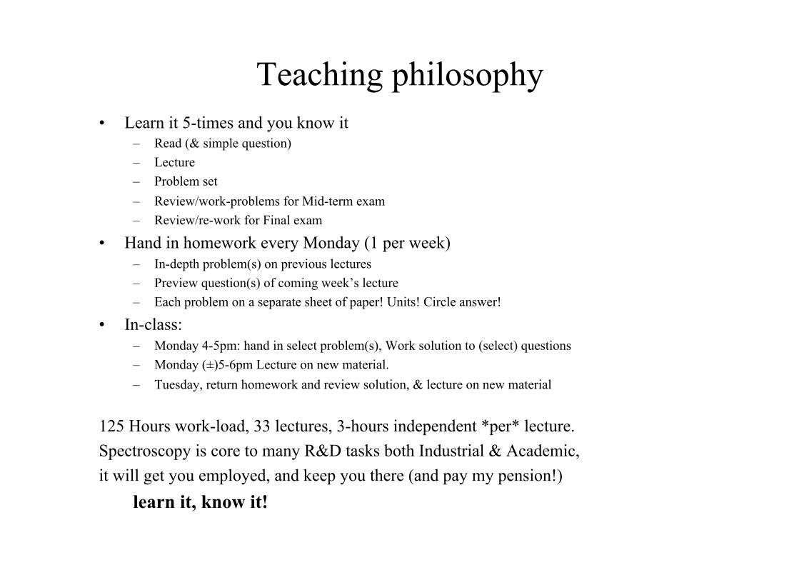
Course Outline

1. Introduction to Spectroscopy

2. Instrumentation

3. Rotational (Microwave) Spectroscopy

4. Vibrational (Infra-Red) Spectroscopy

5. Ro-Vibrational Spectroscopy

6. Raman Spectroscopy

7. Rot / Vib Spectroscopy Techniques

8. Visible/UV Spectroscopy

Exam 1 --------- 5 Nov

Exam 2 --------- 17 Dec

Dates are *targets* only, I will keep you informed.

Assigned problems

1) once per week

2) Due at *beginning* of class

3) 1st type of problem, preview of coming lecture

4) 2nd type of problem, challenging Q on core topics

Grading

80% Final Exam + 20% CA Continuous Assessment:

7.5% for each Mid-term exam (15% total) 5% for Home-Work

Any Questions?

PS 415 Applied Spectroscopy

Name: Bert Ellingboe

Tel: x5314, 087-694-3644

Room: N104

Office Hours: Tues 12-1, Th 1-2, by appointment

Recommended Books

1) Fundamentals of Molecular Spectroscopy C.N.Banwell and E.M.McCash

2) Principles of Instrumental Analysis Skoog, Nieman and Holler

3) Spectrophysics A.Thorne, U.Litzen, S.Johansson

5) Physical Chemistry P.Atkins

4) Modern Spectroscopy (and Basic Atomic and Molecular Spectroscopy)

J.M.Hollas

What is Spectroscopy?

Spectroscopy is the use of the absorption, emission, or scattering of electromagnetic radiation (EMR) by matter to qualitatively or quantitatively study matter or to study dynamical physical processes. Matter can be atoms, molecules, atomic or molecular ions, liquids or solids.

The science of using electromagnetic radiation to probe the properties of atoms, molecules and materials.

The interaction of radiation with matter can cause redirection of the radiation (Scattering) and/or transitions between the energy levels of the atoms or molecules (Absorption or Emission).

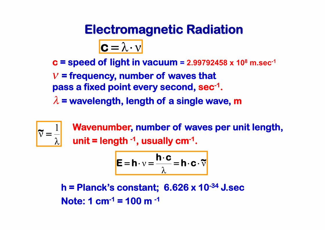
Electromagnetic Radiation

c = speed of light in vacuum = 2.99792458 x 108 m.sec-1

= frequency, number of waves that pass a fixed point every second, sec-1.

= wavelength, length of a single wave, m

νλ ⋅=c

λ1ν =~ Wavenumber, number of waves per unit length,

unit = length -1, usually cm-1.

νλ

ν ~chch

hE ⋅⋅=⋅=⋅=

h = Planck’s constant; 6.626 x 10-34 J.sec

Note: 1 cm-1 = 100 m -1

ν

λ

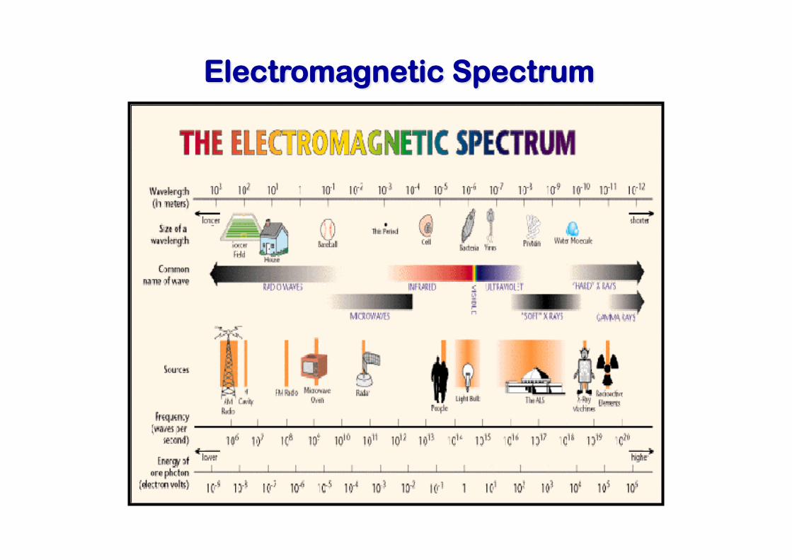
Electromagnetic Spectrum

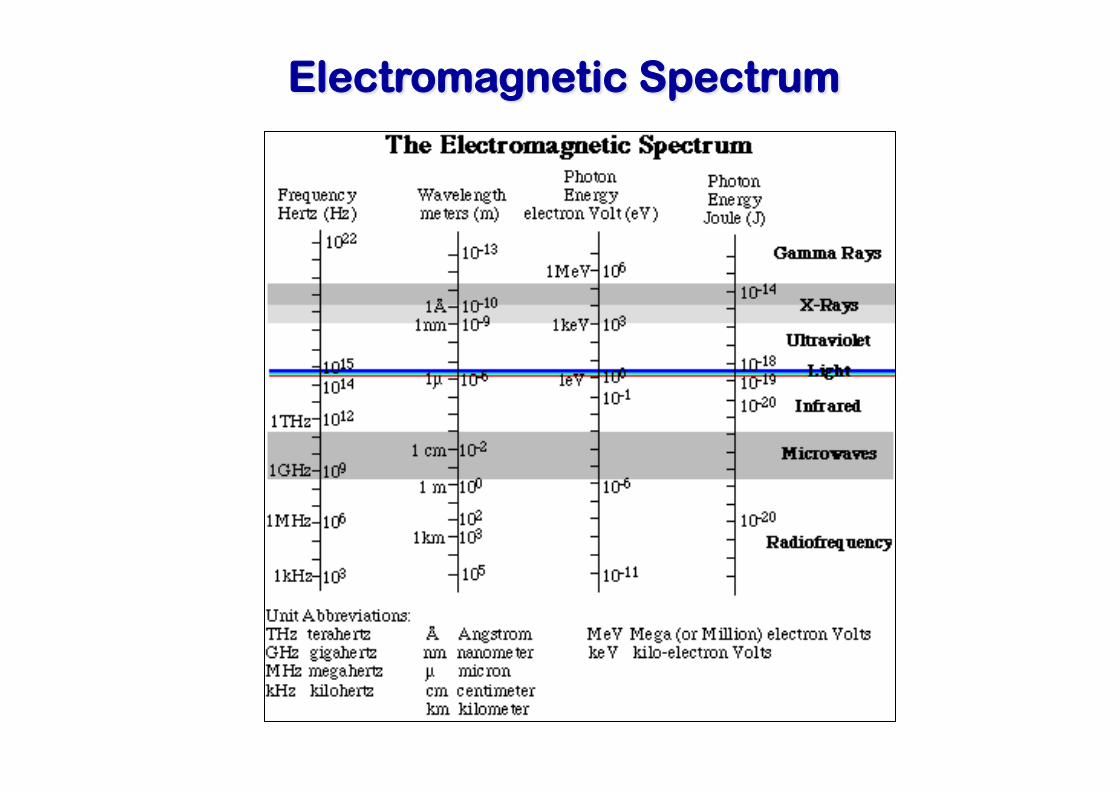
Electromagnetic Spectrum

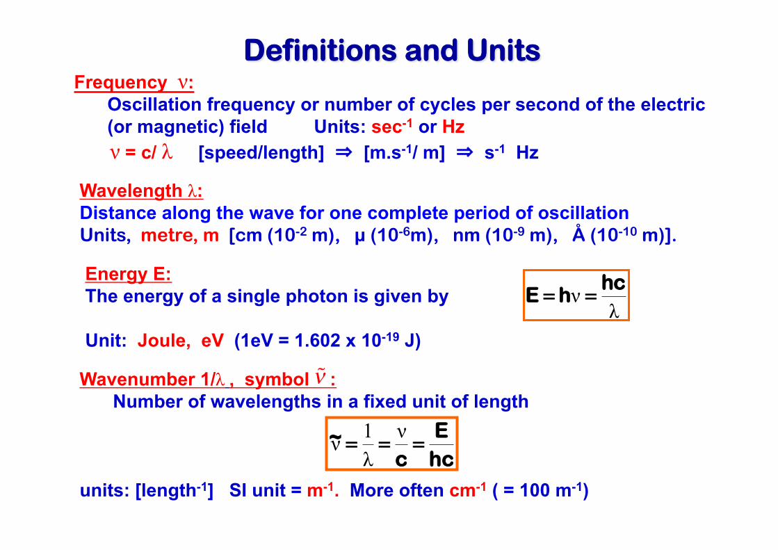
Definitions and Units Frequency ν:

Oscillation frequency or number of cycles per second of the electric (or magnetic) field Units: sec-1 or Hz

ν = c/ λ [speed/length] ⇒ [m.s-1/ m] ⇒ s-1 Hz Wavelength λ: Distance along the wave for one complete period of oscillation Units, metre, m [cm (10-2 m), µ (10-6m), nm (10-9 m), Å (10-10 m)].

Wavenumber 1/λ , symbol : Number of wavelengths in a fixed unit of length

units: [length-1] SI unit = m-1. More often cm-1 ( = 100 m-1)

ν

hcE

c~ === ν

λ1ν

Energy E: The energy of a single photon is given by Unit: Joule, eV (1eV = 1.602 x 10-19 J)

λν hc

hE ==

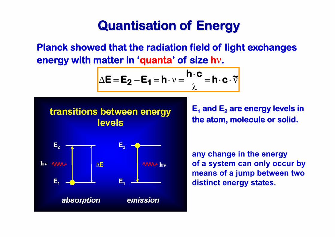
Quantisation of Energy

Planck showed that the radiation field of light exchanges energy with matter in ‘quanta’ of size hν.

νλ

νΔ ~chch

hEEE 12 ⋅⋅=⋅=⋅=−=

E1 and E2 are energy levels in the atom, molecule or solid.

any change in the energy of a system can only occur by means of a jump between two distinct energy states.

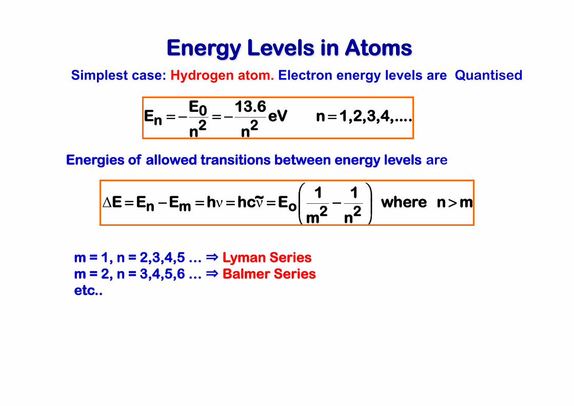
Energy Levels in Atoms Simplest case: Hydrogen atom. Electron energy levels are Quantised

..1,2,3,4,..n eVn

6.13

n

EE

220

n =−=−=

m n where n

1

m

1E~hchEEE

22omn >⎟⎟⎠

⎞⎜⎜⎝

⎛−===−= ννΔ

Energies of allowed transitions between energy levels are

m = 1, n = 2,3,4,5 … ⇒ Lyman Series m = 2, n = 3,4,5,6 … ⇒ Balmer Series etc..

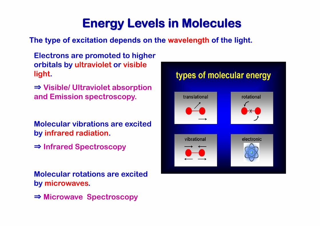
Energy Levels in Molecules

Electrons are promoted to higher orbitals by ultraviolet or visible light. ⇒ Visible/ Ultraviolet absorption and Emission spectroscopy. Molecular vibrations are excited by infrared radiation. ⇒ Infrared Spectroscopy Molecular rotations are excited by microwaves. ⇒ Microwave Spectroscopy

The type of excitation depends on the wavelength of the light.

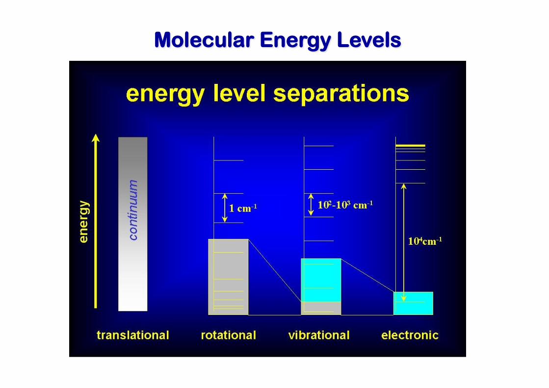
Molecular Energy Levels

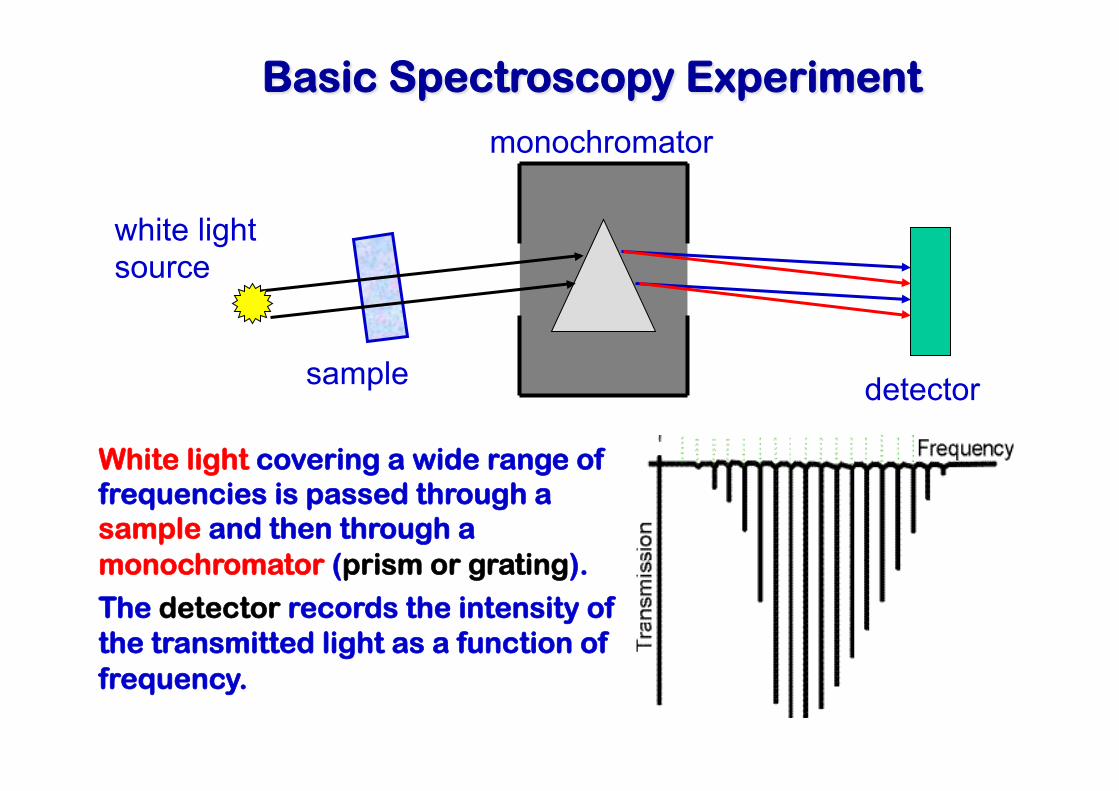
Basic Spectroscopy Experiment

white light source

sample

monochromator

detector

White light covering a wide range of frequencies is passed through a sample and then through a monochromator (prism or grating).

The detector records the intensity of the transmitted light as a function of frequency.

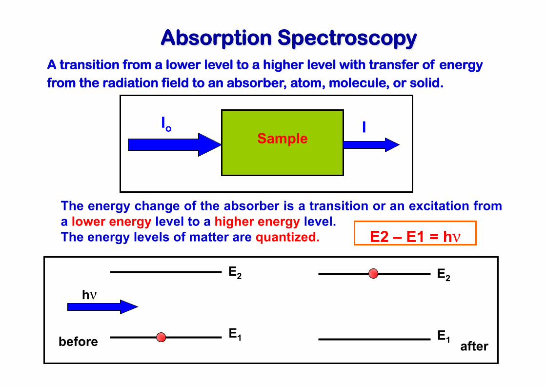
Absorption Spectroscopy

hν E2

E1

E2

E1 before after

Sample

Io I

A transition from a lower level to a higher level with transfer of energy from the radiation field to an absorber, atom, molecule, or solid.

The energy change of the absorber is a transition or an excitation from a lower energy level to a higher energy level. The energy levels of matter are quantized. E2 – E1 = hν

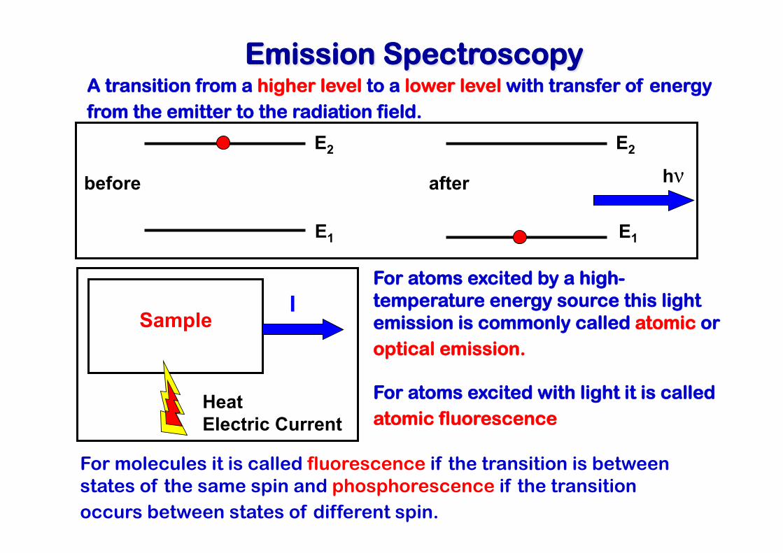
Emission Spectroscopy

E1

E2

E1

hν E2

before after

A transition from a higher level to a lower level with transfer of energy from the emitter to the radiation field.

Sample

I

Heat Electric Current

For atoms excited by a high-temperature energy source this light emission is commonly called atomic or optical emission.

For atoms excited with light it is called atomic fluorescence

For molecules it is called fluorescence if the transition is between states of the same spin and phosphorescence if the transition occurs between states of different spin.

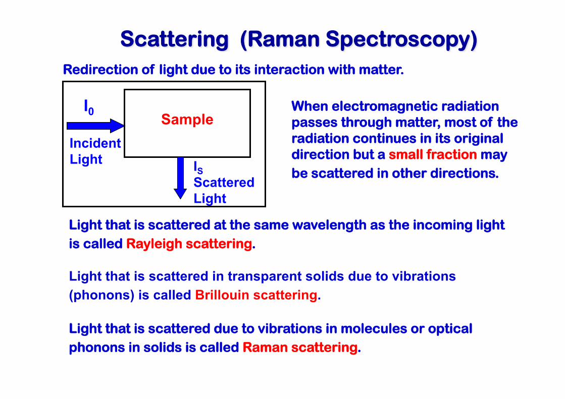
Scattering (Raman Spectroscopy) Redirection of light due to its interaction with matter.

IS Scattered Light

Incident Light

Sample

I0 When electromagnetic radiation passes through matter, most of the radiation continues in its original direction but a small fraction may be scattered in other directions.

Light that is scattered at the same wavelength as the incoming light is called Rayleigh scattering.

Light that is scattered in transparent solids due to vibrations (phonons) is called Brillouin scattering.

Light that is scattered due to vibrations in molecules or optical phonons in solids is called Raman scattering.

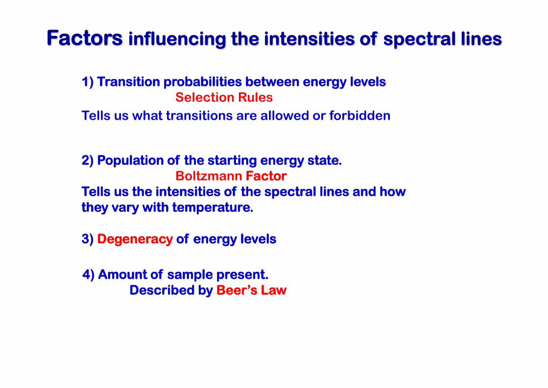
Factors influencing the intensities of spectral lines

1) Transition probabilities between energy levels Selection Rules

Tells us what transitions are allowed or forbidden

2) Population of the starting energy state. Boltzmann Factor

Tells us the intensities of the spectral lines and how they vary with temperature.

3) Degeneracy of energy levels

4) Amount of sample present. Described by Beer’s Law

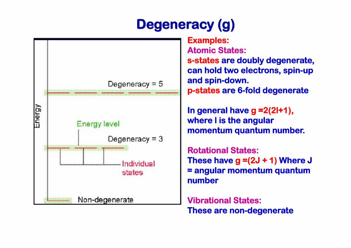
Degeneracy (g) Examples: Atomic States: s-states are doubly degenerate, can hold two electrons, spin-up and spin-down. p-states are 6-fold degenerate In general have g =2(2l+1), where l is the angular momentum quantum number.

Rotational States: These have g =(2J + 1) Where J = angular momentum quantum number Vibrational States: These are non-degenerate

Boltzmann Factor

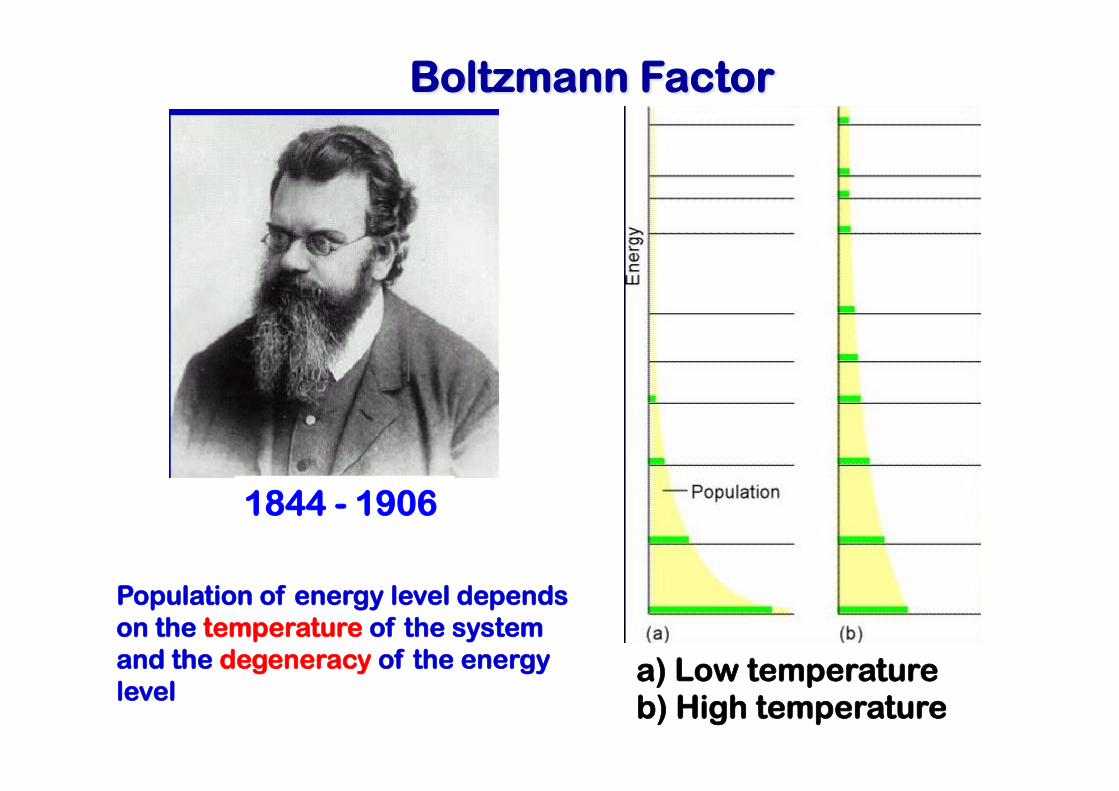
1844 - 1906

Population of energy level depends on the temperature of the system and the degeneracy of the energy level a) Low temperature

b) High temperature

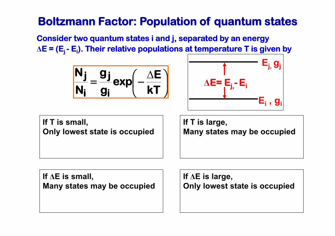
Boltzmann Factor: Population of quantum states Consider two quantum states i and j, separated by an energy ΔE = (Ej - Ei). Their relative populations at temperature T is given by

⎟⎠⎞⎜

⎝⎛−=

kTE

expg

g

N

N

i

j

i

j Δ

If T is small, Only lowest state is occupied

If T is large, Many states may be occupied

If ΔE is large, Only lowest state is occupied

If ΔE is small, Many states may be occupied

Ej, gj

Ei , gi

ΔE= Ej,- Ei

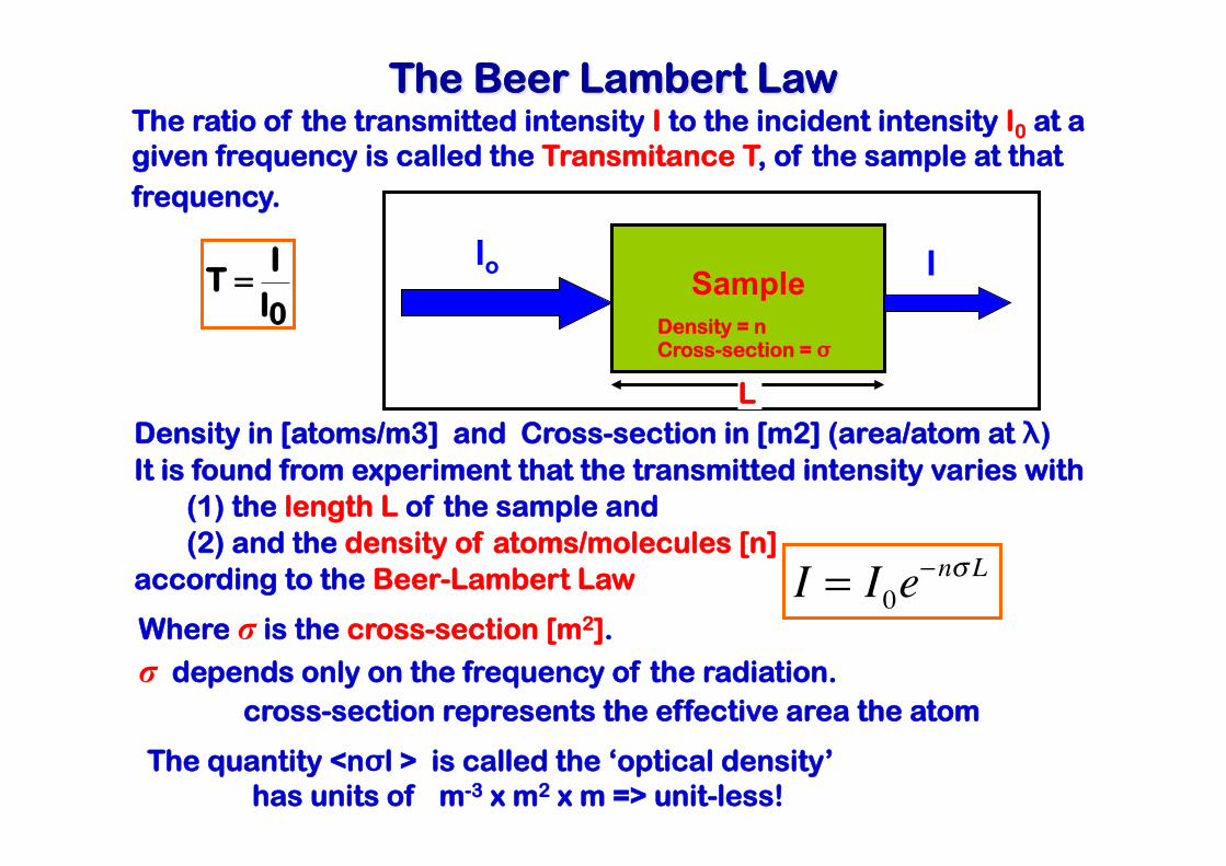
The Beer Lambert Law The ratio of the transmitted intensity I to the incident intensity I0 at a given frequency is called the Transmitance T, of the sample at that frequency.

0II

T =

Density in [atoms/m3] and Cross-section in [m2] (area/atom at λ) It is found from experiment that the transmitted intensity varies with

(1) the length L of the sample and (2) and the density of atoms/molecules [n]

according to the Beer-Lambert Law I = I0e−nσ L

Where σ is the cross-section [m2].

σ depends only on the frequency of the radiation. cross-section represents the effective area the atom

The quantity <nσl > is called the ‘optical density’ has units of m-3 x m2 x m => unit-less!

Sample

Io I

L Density = n Cross-section = σ

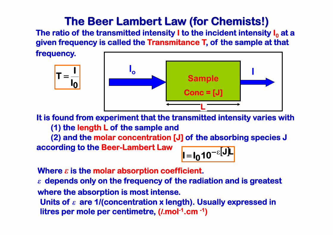
The Beer Lambert Law (for Chemists!) The ratio of the transmitted intensity I to the incident intensity I0 at a given frequency is called the Transmitance T, of the sample at that frequency.

0II

T =

It is found from experiment that the transmitted intensity varies with (1) the length L of the sample and (2) and the molar concentration [J] of the absorbing species J

according to the Beer-Lambert Law [ ]LJ010II ε−=

Where ε is the molar absorption coefficient. ε depends only on the frequency of the radiation and is greatest where the absorption is most intense. Units of ε are 1/(concentration x length). Usually expressed in litres per mole per centimetre, (l.mol-1.cm -1)

Sample

Io I

L Conc = [J]

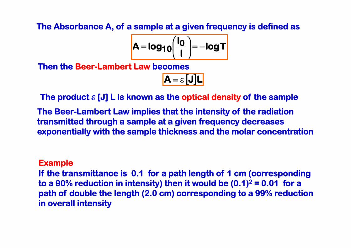
The Absorbance A, of a sample at a given frequency is defined as

TlogII

logA 010 −=⎟

⎠⎞⎜

⎝⎛=

Then the Beer-Lambert Law becomes

[ ]L J A ε=

The product ε [J] L is known as the optical density of the sample

The Beer-Lambert Law implies that the intensity of the radiation transmitted through a sample at a given frequency decreases exponentially with the sample thickness and the molar concentration

Example If the transmittance is 0.1 for a path length of 1 cm (corresponding to a 90% reduction in intensity) then it would be (0.1)2 = 0.01 for a path of double the length (2.0 cm) corresponding to a 99% reduction in overall intensity

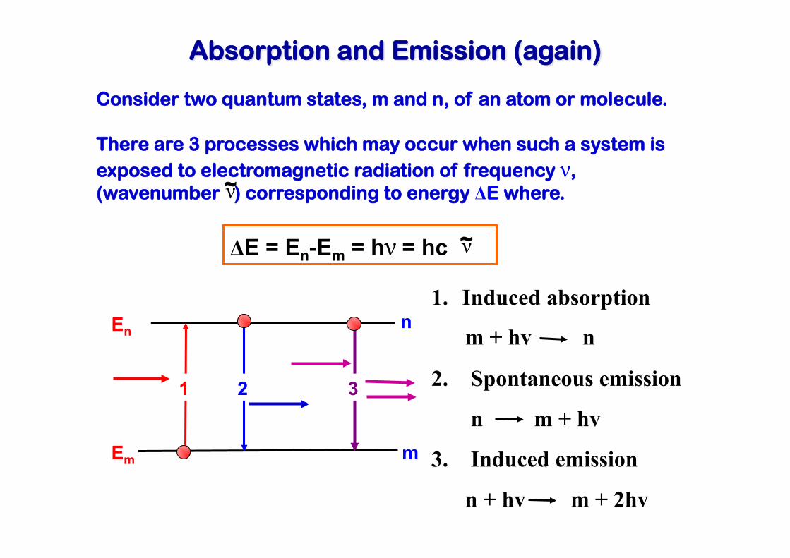
Absorption and Emission (again)

ΔE = En-Em = hν = hc ν~

1 2 3

En

Em

n

m

Consider two quantum states, m and n, of an atom or molecule. There are 3 processes which may occur when such a system is exposed to electromagnetic radiation of frequency ν, (wavenumber ) corresponding to energy ΔE where. ν~

1.  Induced absorption

m + hv n

2. Spontaneous emission

n m + hv

3. Induced emission

n + hv m + 2hv

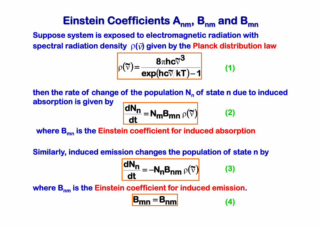
Einstein Coefficients Anm, Bnm and Bmn Suppose system is exposed to electromagnetic radiation with spectral radiation density ρ( ) given by the Planck distribution law ν

( ) ( ) 1kT~hcexp

~hc8~3

−=

ννπνρ

then the rate of change of the population Nn of state n due to induced absorption is given by

( )νρ ~BNdt

dN mnm

n =

where Bmn is the Einstein coefficient for induced absorption

Similarly, induced emission changes the population of state n by

( )νρ ~BNdt

dN nmn

n −=

where Bnm is the Einstein coefficient for induced emission. nmmn BB =

(1)

(2)

(3)

(4)

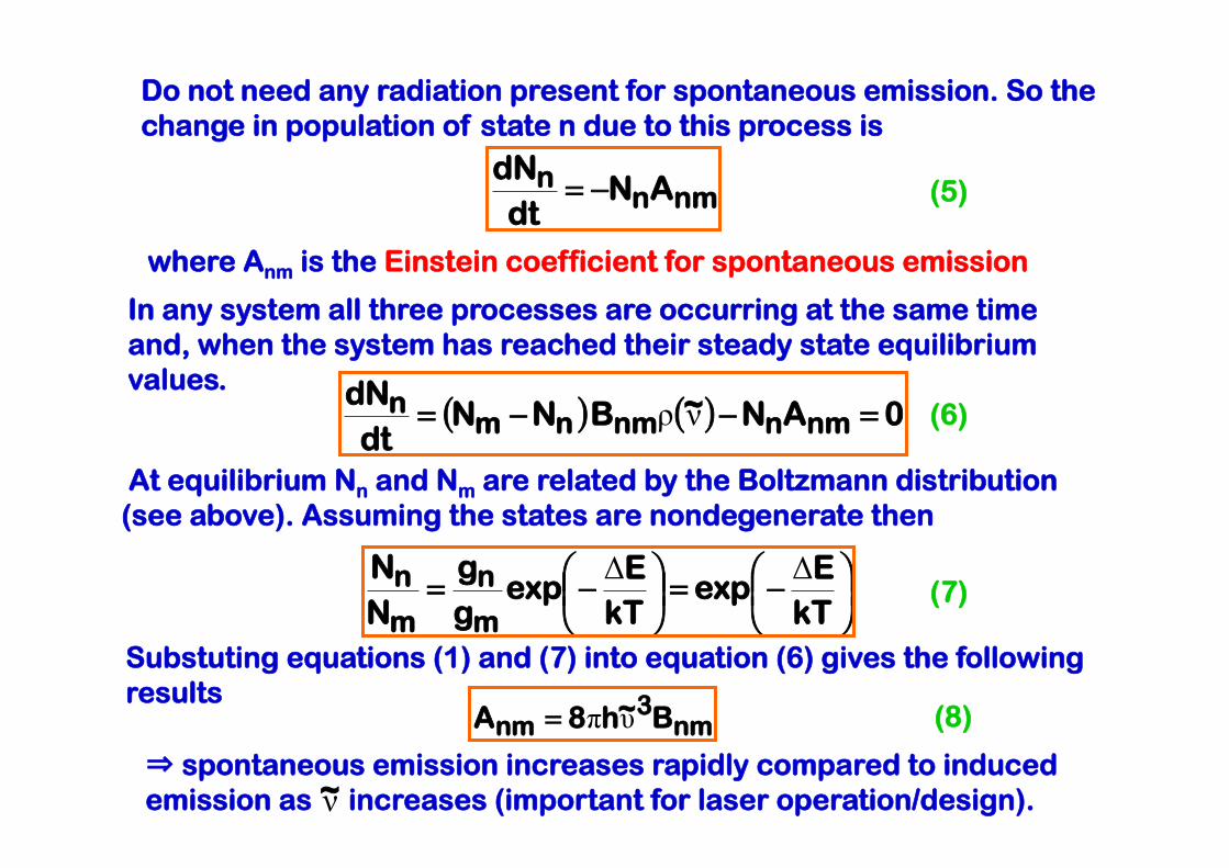
Do not need any radiation present for spontaneous emission. So the change in population of state n due to this process is

nmnn AN

dtdN −=

where Anm is the Einstein coefficient for spontaneous emission In any system all three processes are occurring at the same time and, when the system has reached their steady state equilibrium values.

( ) ( ) 0AN~B NNdt

dNnmnnmnm

n =−−= νρ

At equilibrium Nn and Nm are related by the Boltzmann distribution (see above). Assuming the states are nondegenerate then

⎟⎠⎞⎜

⎝⎛−=⎟

⎠⎞⎜

⎝⎛−=

kTE

expkTE

expgg

NN

m

n

m

n ΔΔ

Substuting equations (1) and (7) into equation (6) gives the following results

(5)

(6)

(7)

nm3

nm B~h8A υπ= (8) ⇒ spontaneous emission increases rapidly compared to induced emission as increases (important for laser operation/design). ν~

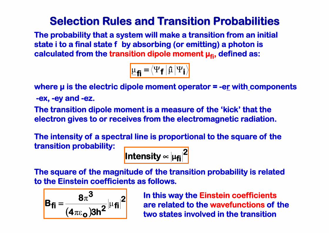
Selection Rules and Transition Probabilities The probability that a system will make a transition from an initial state i to a final state f by absorbing (or emitting) a photon is calculated from the transition dipole moment µfi, defined as:

iffi ˆ Ψ µ Ψµ =

where µ is the electric dipole moment operator = -er with components

-ex, -ey and -ez. The transition dipole moment is a measure of the ‘kick’ that the electron gives to or receives from the electromagnetic radiation.

The intensity of a spectral line is proportional to the square of the transition probability:

2

fiμ Intensity ∝

The square of the magnitude of the transition probability is related to the Einstein coefficients as follows.

( )2

fi2o

3

fih34

8B µ

πε

π=In this way the Einstein coefficients are related to the wavefunctions of the two states involved in the transition

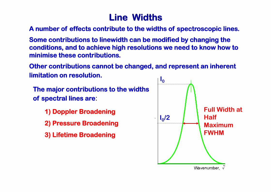
Line Widths A number of effects contribute to the widths of spectroscopic lines.

Some contributions to linewidth can be modified by changing the conditions, and to achieve high resolutions we need to know how to minimise these contributions.

Other contributions cannot be changed, and represent an inherent limitation on resolution.

The major contributions to the widths of spectral lines are:

1) Doppler Broadening

2) Pressure Broadening

3) Lifetime Broadening

I0

I0/2 Full Width at Half Maximum FWHM

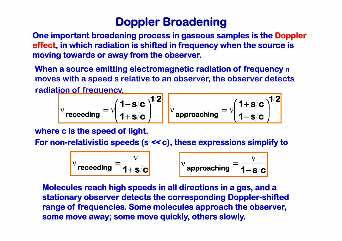
Doppler Broadening One important broadening process in gaseous samples is the Doppler effect, in which radiation is shifted in frequency when the source is moving towards or away from the observer.

When a source emitting electromagnetic radiation of frequency n moves with a speed s relative to an observer, the observer detects radiation of frequency.

21

cs1cs1

receeding ⎟⎠⎞⎜

⎝⎛

+−= νν

21

cs1cs1

gapproachin ⎟⎠⎞⎜

⎝⎛

−+= νν

where c is the speed of light. For non-relativistic speeds (s << c), these expressions simplify to

cs1receeding += νν

cs1gapproachin −= νν

Molecules reach high speeds in all directions in a gas, and a stationary observer detects the corresponding Doppler-shifted range of frequencies. Some molecules approach the observer, some move away; some move quickly, others slowly.

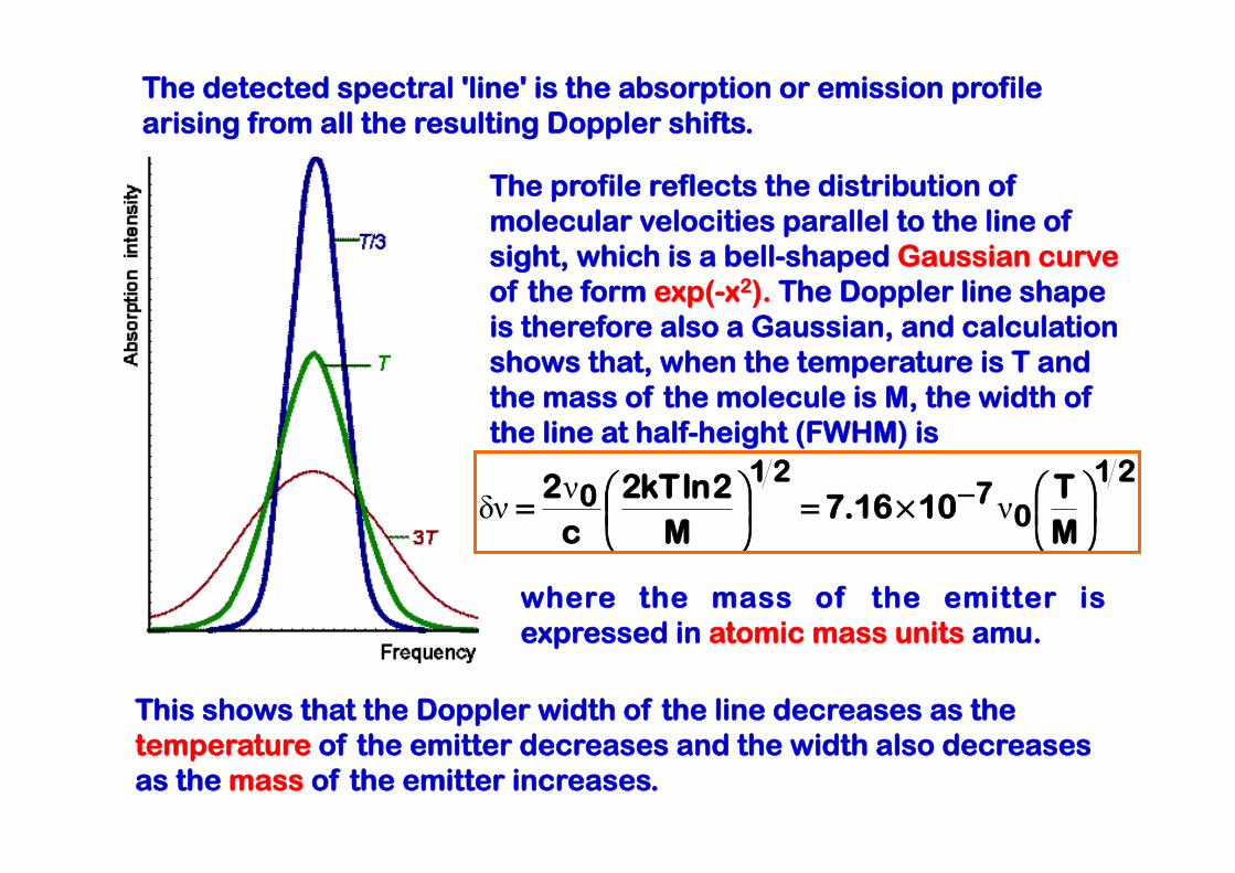
The detected spectral 'line' is the absorption or emission profile arising from all the resulting Doppler shifts.

The profile reflects the distribution of molecular velocities parallel to the line of sight, which is a bell-shaped Gaussian curve of the form exp(-x2). The Doppler line shape is therefore also a Gaussian, and calculation shows that, when the temperature is T and the mass of the molecule is M, the width of the line at half-height (FWHM) is

21

07

210

MT

1016.7M

2lnkT2c

2⎟⎠⎞⎜

⎝⎛×=⎟

⎠⎞⎜

⎝⎛= − ννδν

where the mass of the emitter is expressed in atomic mass units amu.

This shows that the Doppler width of the line decreases as the temperature of the emitter decreases and the width also decreases as the mass of the emitter increases.

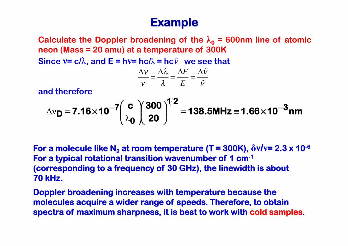
Example Calculate the Doppler broadening of the λ0 = 600nm line of atomic neon (Mass = 20 amu) at a temperature of 300K Since ν= c/λ, and E = hν= hc/λ = hc we see that

and therefore

Δνν

= Δλλ

= ΔEE

= Δ νν

nm1066.1MHz5.13820300c

1016.7 321

0

7D

−− ×≡=⎟⎠⎞⎜

⎝⎛⎟⎟⎠⎞

⎜⎜⎝⎛×=λ

Δν

For a molecule like N2 at room temperature (T = 300K), δν/ν= 2.3 x 10-6 For a typical rotational transition wavenumber of 1 cm-1 (corresponding to a frequency of 30 GHz), the linewidth is about 70 kHz.

Doppler broadening increases with temperature because the molecules acquire a wider range of speeds. Therefore, to obtain spectra of maximum sharpness, it is best to work with cold samples.

ν

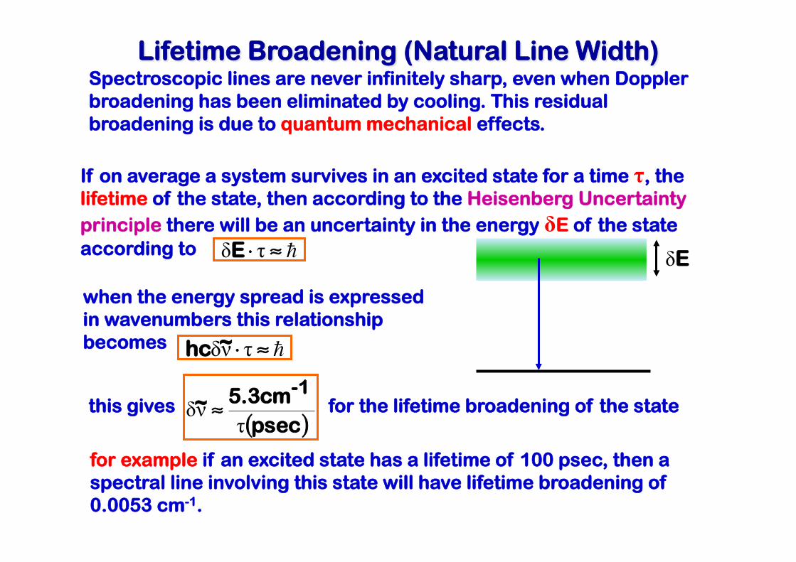
Lifetime Broadening (Natural Line Width) Spectroscopic lines are never infinitely sharp, even when Doppler broadening has been eliminated by cooling. This residual broadening is due to quantum mechanical effects.

If on average a system survives in an excited state for a time τ, the lifetime of the state, then according to the Heisenberg Uncertainty principle there will be an uncertainty in the energy δE of the state according to E ≈⋅ τδ

when the energy spread is expressed in wavenumbers this relationship becomes ~hc ≈⋅ τνδ

this gives ( )psec

.3cm5~1-

τνδ ≈ for the lifetime broadening of the state

for example if an excited state has a lifetime of 100 psec, then a spectral line involving this state will have lifetime broadening of 0.0053 cm-1.

E δ

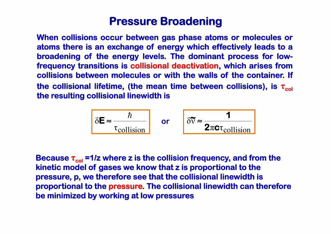
When collisions occur between gas phase atoms or molecules or atoms there is an exchange of energy which effectively leads to a broadening of the energy levels. The dominant process for low-frequency transitions is collisional deactivation, which arises from collisions between molecules or with the walls of the container. If the collisional lifetime, (the mean time between collisions), is τcol the resulting collisional linewidth is

Pressure Broadening

Because τcol =1/z where z is the collision frequency, and from the kinetic model of gases we know that z is proportional to the pressure, p, we therefore see that the collisional linewidth is proportional to the pressure. The collisional linewidth can therefore be minimized by working at low pressures

E collisionτ

δ ≈ c2

1~ collisionτπ

νδ ≈or