Introduction and Kinematics Lecture 1

� First half of this lecture is a quick overview of physics—the bottom line.

� Second half is our initial steps into kinematics, the vocabulary of motion. The key concepts are velocity andacceleration.

� We are skipping vectors for now (we will cover that next week in the context of force).

1

What We Know Now Lecture 1

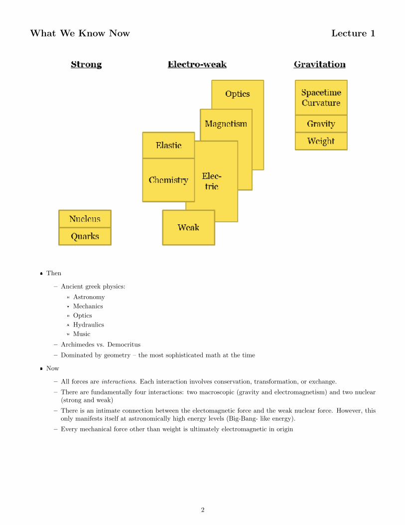
� Then

– Ancient greek physics:

* Astronomy

* Mechanics

* Optics

* Hydraulics

* Music

– Archimedes vs. Democritus

– Dominated by geometry – the most sophisticated math at the time

� Now

– All forces are interactions. Each interaction involves conservation, transformation, or exchange.

– There are fundamentally four interactions: two macroscopic (gravity and electromagnetism) and two nuclear(strong and weak)

– There is an intimate connection between the electomagnetic force and the weak nuclear force. However, thisonly manifests itself at astronomically high energy levels (Big-Bang- like energy).

– Every mechanical force other than weight is ultimately electromagnetic in origin

2

Ultimately, It’s All Mechanics Lecture 1

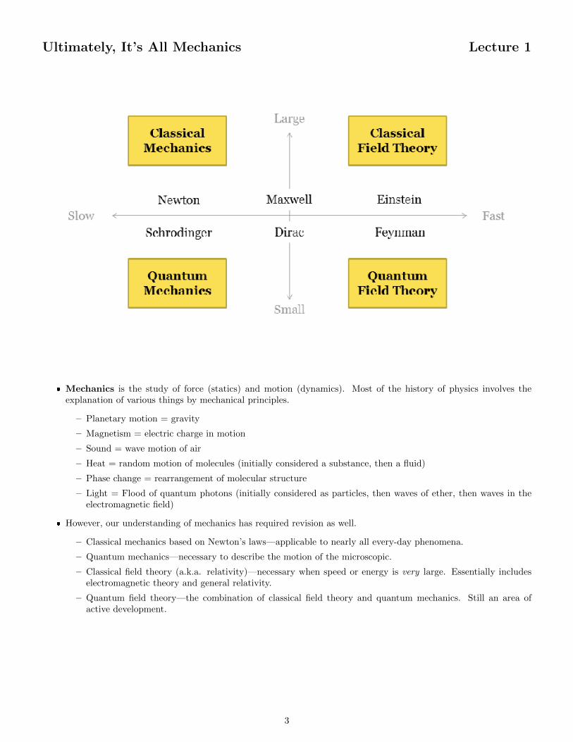
� Mechanics is the study of force (statics) and motion (dynamics). Most of the history of physics involves theexplanation of various things by mechanical principles.

– Planetary motion = gravity

– Magnetism = electric charge in motion

– Sound = wave motion of air

– Heat = random motion of molecules (initially considered a substance, then a fluid)

– Phase change = rearrangement of molecular structure

– Light = Flood of quantum photons (initially considered as particles, then waves of ether, then waves in theelectromagnetic field)

� However, our understanding of mechanics has required revision as well.

– Classical mechanics based on Newton’s laws—applicable to nearly all every-day phenomena.

– Quantum mechanics—necessary to describe the motion of the microscopic.

– Classical field theory (a.k.a. relativity)—necessary when speed or energy is very large. Essentially includeselectromagnetic theory and general relativity.

– Quantum field theory—the combination of classical field theory and quantum mechanics. Still an area ofactive development.

3

Particle is the Simplest System of All Lecture 1

� Until we get to “modern physics” in the third term, everything from now on is classical mechanics.

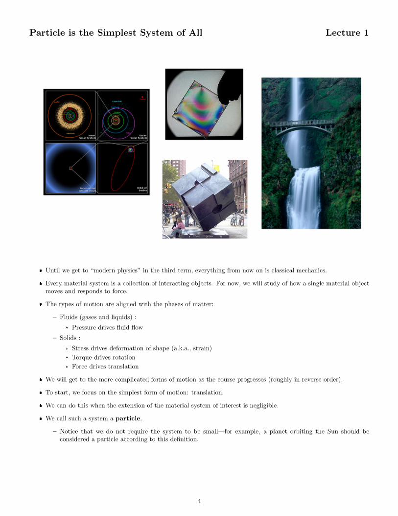
� Every material system is a collection of interacting objects. For now, we will study of how a single material objectmoves and responds to force.

� The types of motion are aligned with the phases of matter:

– Fluids (gases and liquids) :

* Pressure drives fluid flow

– Solids :

* Stress drives deformation of shape (a.k.a., strain)

* Torque drives rotation

* Force drives translation

� We will get to the more complicated forms of motion as the course progresses (roughly in reverse order).

� To start, we focus on the simplest form of motion: translation.

� We can do this when the extension of the material system of interest is negligible.

� We call such a system a particle.

– Notice that we do not require the system to be small—for example, a planet orbiting the Sun should beconsidered a particle according to this definition.

4

Units and Measurement Lecture 1

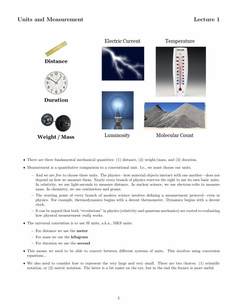
� There are three fundamental mechanical quantities: (1) distance, (2) weight/mass, and (3) duration.

� Measurement is a quantitative comparison to a conventional unit. I.e., we must choose our units.

– And we are free to choose these units. The physics—how material objects interact with one another—does notdepend on how we measure them. Nearly every branch of physics reserves the right to use its own basic units.In relativity, we use light-seconds to measure distance. In nuclear science, we use electron-volts to measuremass. In chemistry, we use centimeters and grams.

– The starting point of every branch of modern science involves defining a measurement protocol—even inphysics. For example, thermodynamics begins with a decent thermometer. Dynamics begins with a decentclock.

– It can be argued that both “revolutions” in physics (relativity and quantum mechanics) are rooted re-evaluatinghow physical measurement really works.

� The universal convention is to use SI units, a.k.a., MKS units:

– For distance we use the meter

– For mass we use the kilogram

– For duration we use the second

� This means we need to be able to convert between different systems of units. This involves using conversionequations...

� We also need to consider how to represent the very large and very small. There are two choices: (1) scientificnotation, or (2) metric notation. The latter is a bit easier on the eye, but in the end the former is more useful.

5

Velocity is Change in Position Lecture 1

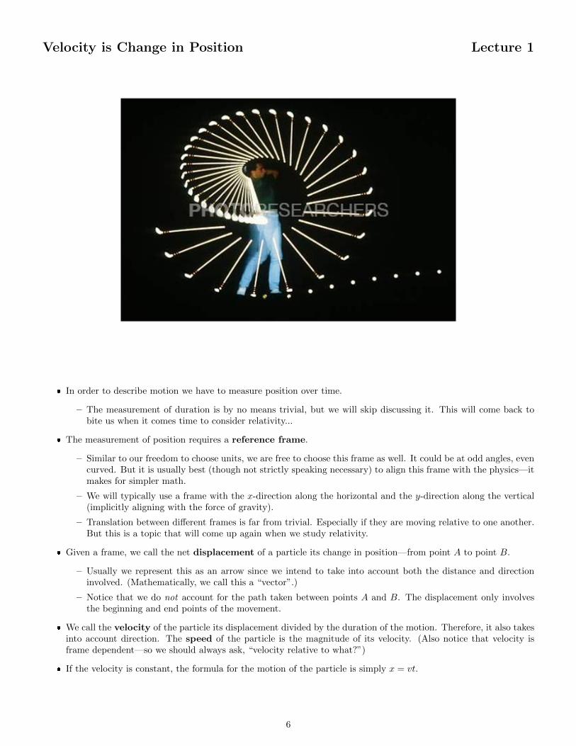
� In order to describe motion we have to measure position over time.

– The measurement of duration is by no means trivial, but we will skip discussing it. This will come back tobite us when it comes time to consider relativity...

� The measurement of position requires a reference frame.

– Similar to our freedom to choose units, we are free to choose this frame as well. It could be at odd angles, evencurved. But it is usually best (though not strictly speaking necessary) to align this frame with the physics—itmakes for simpler math.

– We will typically use a frame with the x-direction along the horizontal and the y-direction along the vertical(implicitly aligning with the force of gravity).

– Translation between different frames is far from trivial. Especially if they are moving relative to one another.But this is a topic that will come up again when we study relativity.

� Given a frame, we call the net displacement of a particle its change in position—from point A to point B.

– Usually we represent this as an arrow since we intend to take into account both the distance and directioninvolved. (Mathematically, we call this a “vector”.)

– Notice that we do not account for the path taken between points A and B. The displacement only involvesthe beginning and end points of the movement.

� We call the velocity of the particle its displacement divided by the duration of the motion. Therefore, it also takesinto account direction. The speed of the particle is the magnitude of its velocity. (Also notice that velocity isframe dependent—so we should always ask, “velocity relative to what?”)

� If the velocity is constant, the formula for the motion of the particle is simply x = vt.

6

Average vs. Instantaneous Velocity Lecture 1

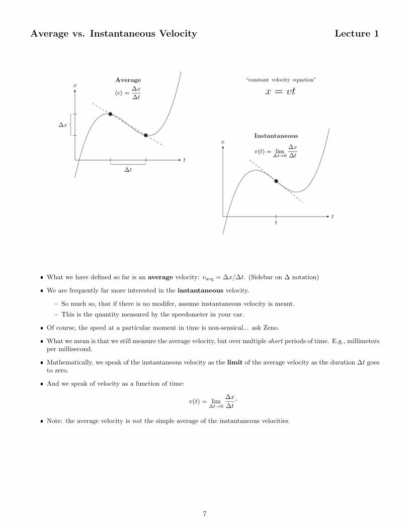
� What we have defined so far is an average velocity: vavg = ∆x/∆t. (Sidebar on ∆ notation)

� We are frequently far more interested in the instantaneous velocity.

– So much so, that if there is no modifer, assume instantaneous velocity is meant.

– This is the quantity measured by the speedometer in your car.

� Of course, the speed at a particular moment in time is non-sensical... ask Zeno.

� What we mean is that we still measure the average velocity, but over multiple short periods of time. E.g., millimetersper millisecond.

� Mathematically, we speak of the instantaneous velocity as the limit of the average velocity as the duration ∆t goesto zero.

� And we speak of velocity as a function of time:

v(t) = lim∆t→0

∆x

∆t‘

� Note: the average velocity is not the simple average of the instantaneous velocities.

7

Sidebar: The Importance of Neglect Lecture 1

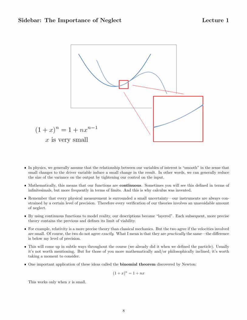
� In physics, we generally assume that the relationship between our variables of interest is “smooth” in the sense thatsmall changes to the driver variable induce a small change in the result. In other words, we can generally reducethe size of the variance on the output by tightening our control on the input.

� Mathematically, this means that our functions are continuous. Sometimes you will see this defined in terms ofinfinitesimals, but more frequently in terms of limits. And this is why calculus was invented.

� Remember that every physical measurement is surrounded a small uncertainty—our instruments are always con-strained by a certain level of precision. Therefore every verification of our theories involves an unavoidable amountof neglect.

� By using continuous functions to model reality, our descriptions become “layered”. Each subsequent, more precisetheory contains the previous and defines its limit of viability.

� For example, relativity is a more precise theory than classical mechanics. But the two agree if the velocities involvedare small. Of course, the two do not agree exactly. What I mean is that they are practically the same—the differenceis below my level of precision.

� This will come up in subtle ways throughout the course (we already did it when we defined the particle). Usuallyit’s not worth mentioning. But for those of you more mathematically and/or philosophically inclined, it’s worthtaking a moment to consider.

� One important application of these ideas called the binomial theorem discovered by Newton:

(1 + x)n = 1 + nx

This works only when x is small.

8

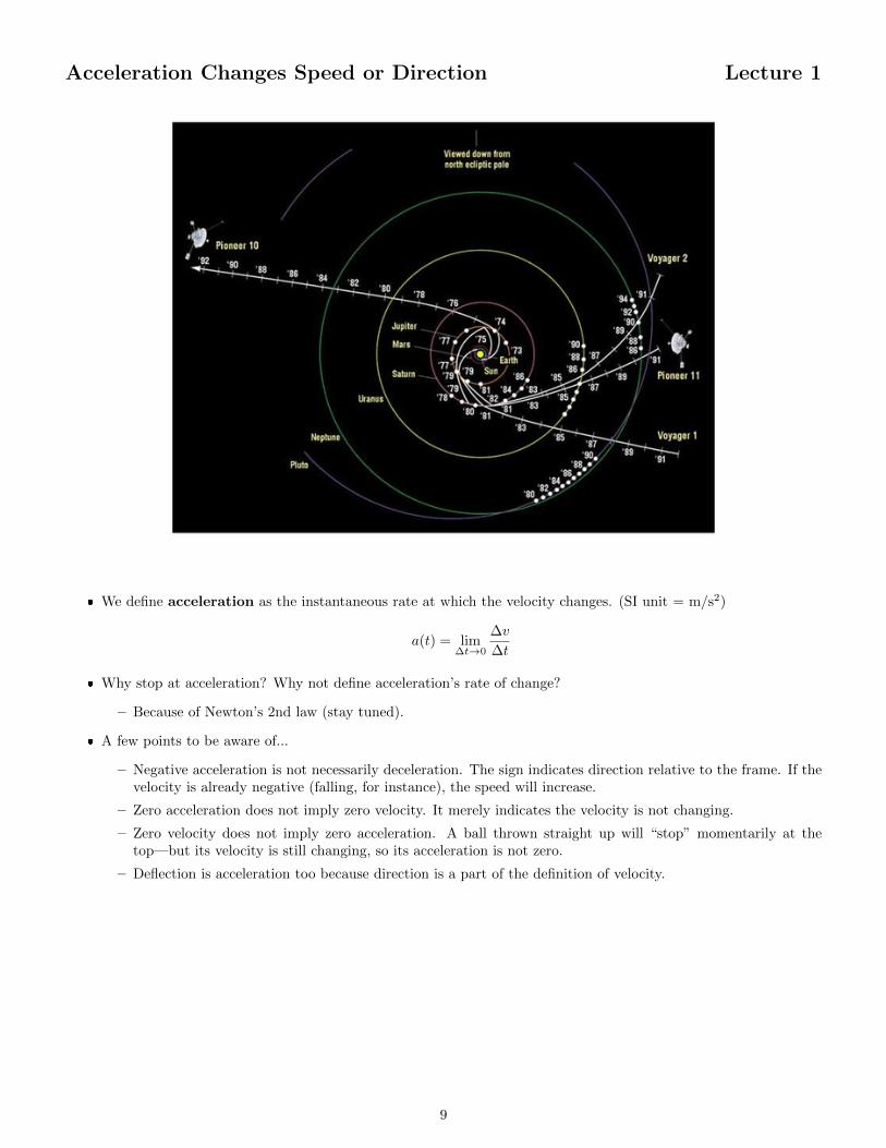
Acceleration Changes Speed or Direction Lecture 1

� We define acceleration as the instantaneous rate at which the velocity changes. (SI unit = m/s2)

a(t) = lim∆t→0

∆v

∆t

� Why stop at acceleration? Why not define acceleration’s rate of change?

– Because of Newton’s 2nd law (stay tuned).

� A few points to be aware of...

– Negative acceleration is not necessarily deceleration. The sign indicates direction relative to the frame. If thevelocity is already negative (falling, for instance), the speed will increase.

– Zero acceleration does not imply zero velocity. It merely indicates the velocity is not changing.

– Zero velocity does not imply zero acceleration. A ball thrown straight up will “stop” momentarily at thetop—but its velocity is still changing, so its acceleration is not zero.

– Deflection is acceleration too because direction is a part of the definition of velocity.

9

Acceleration Due to Gravity Lecture 2

� This lecture covers the “meat” of Chapters 2 and 3 from the book. I am deliberately skipping vectors again—youwill have to bear with me.

� We will cover the basics of constant acceleration (of which free-fall is the prime example). The center of this analysisis five key equations which we will learn to use and apply to a variety of problems including the projectile.

� We will also discuss (qualitatively) the impact of air drag on the motion of projectiles.

10

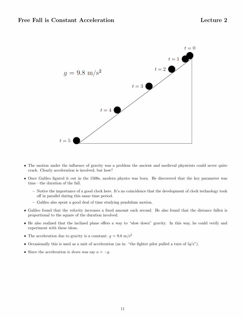
Free Fall is Constant Acceleration Lecture 2

� The motion under the influence of gravity was a problem the ancient and medieval physicists could never quitecrack. Clearly acceleration is involved, but how?

� Once Galileo figured it out in the 1500s, modern physics was born. He discovered that the key parameter wastime—the duration of the fall.

– Notice the importance of a good clock here. It’s no coincidence that the development of clock technology tookoff in parallel during this same time period.

– Galileo also spent a good deal of time studying pendulum motion.

� Galileo found that the velocity increases a fixed amount each second. He also found that the distance fallen isproportional to the square of the duration involved.

� He also realized that the inclined plane offers a way to “slow down” gravity. In this way, he could verify andexperiment with these ideas.

� The acceleration due to gravity is a constant: g = 9.8 m/s2

� Occasionally this is used as a unit of acceleration (as in: “the fighter pilot pulled a turn of 5g’s”).

� Since the acceleration is down was say a = −g.

11

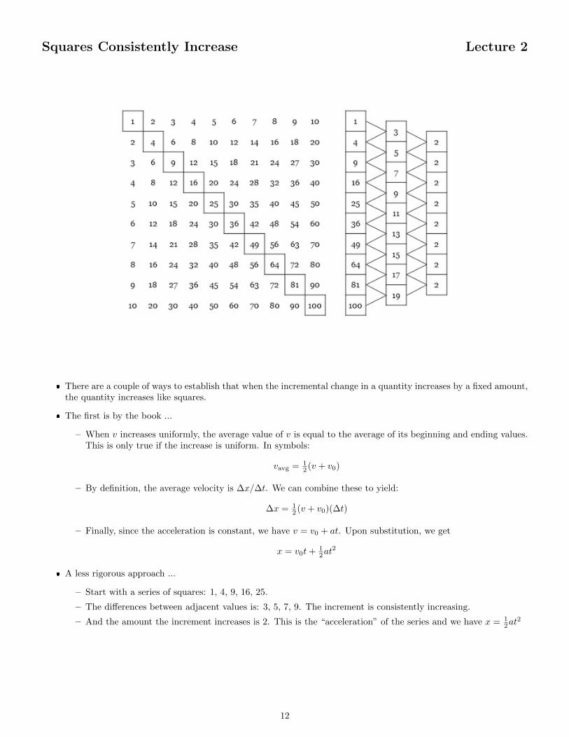
Squares Consistently Increase Lecture 2

� There are a couple of ways to establish that when the incremental change in a quantity increases by a fixed amount,the quantity increases like squares.

� The first is by the book ...

– When v increases uniformly, the average value of v is equal to the average of its beginning and ending values.This is only true if the increase is uniform. In symbols:

vavg = 12 (v + v0)

– By definition, the average velocity is ∆x/∆t. We can combine these to yield:

∆x = 12 (v + v0)(∆t)

– Finally, since the acceleration is constant, we have v = v0 + at. Upon substitution, we get

x = v0t+ 12at

2

� A less rigorous approach ...

– Start with a series of squares: 1, 4, 9, 16, 25.

– The differences between adjacent values is: 3, 5, 7, 9. The increment is consistently increasing.

– And the amount the increment increases is 2. This is the “acceleration” of the series and we have x = 12at

2

12

Equations of Constant Acceleration Lecture 2

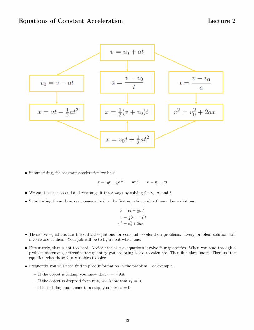
� Summarizing, for constant acceleration we have

x = v0t+ 12at

2 and v = v0 + at

� We can take the second and rearrange it three ways by solving for v0, a, and t.

� Substituting these three rearrangements into the first equation yields three other variations:

x = vt− 12at

2

x = 12 (v + v0)t

v2 = v20 + 2ax

� These five equations are the critical equations for constant acceleration problems. Every problem solution willinvolve one of them. Your job will be to figure out which one.

� Fortunately, that is not too hard. Notice that all five equations involve four quantities. When you read through aproblem statement, determine the quantity you are being asked to calculate. Then find three more. Then use theequation with those four variables to solve.

� Frequently you will need find implied information in the problem. For example,

– If the object is falling, you know that a = −9.8.

– If the object is dropped from rest, you know that v0 = 0.

– If it is sliding and comes to a stop, you have v = 0.

13

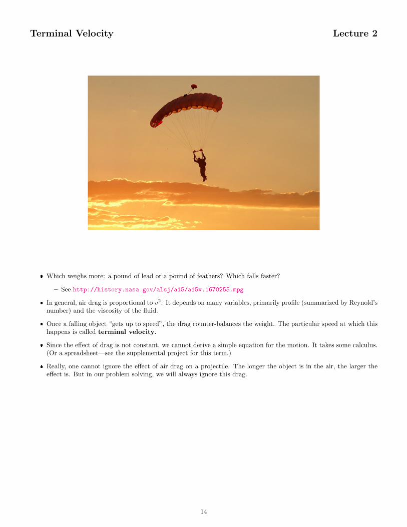
Terminal Velocity Lecture 2

� Which weighs more: a pound of lead or a pound of feathers? Which falls faster?

– See http://history.nasa.gov/alsj/a15/a15v.1670255.mpg

� In general, air drag is proportional to v2. It depends on many variables, primarily profile (summarized by Reynold’snumber) and the viscosity of the fluid.

� Once a falling object “gets up to speed”, the drag counter-balances the weight. The particular speed at which thishappens is called terminal velocity.

� Since the effect of drag is not constant, we cannot derive a simple equation for the motion. It takes some calculus.(Or a spreadsheet—see the supplemental project for this term.)

� Really, one cannot ignore the effect of air drag on a projectile. The longer the object is in the air, the larger theeffect is. But in our problem solving, we will always ignore this drag.

14

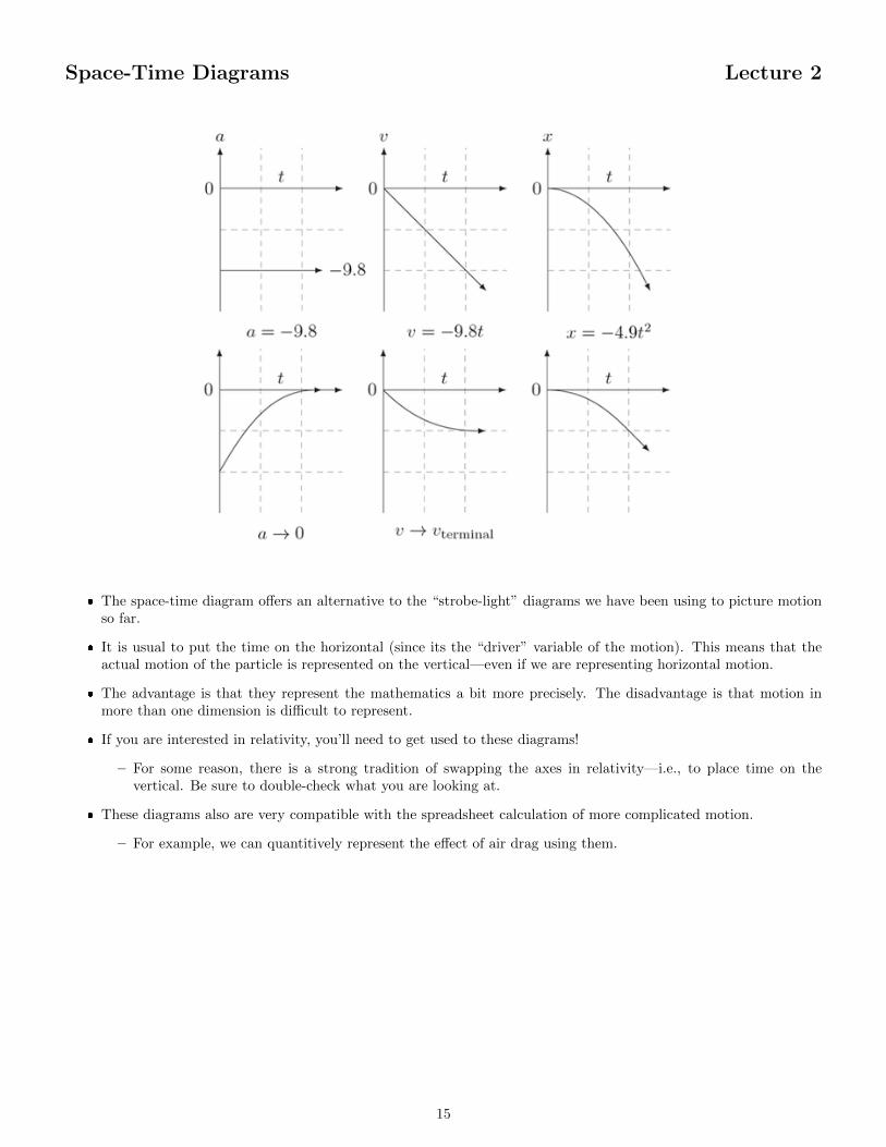
Space-Time Diagrams Lecture 2

� The space-time diagram offers an alternative to the “strobe-light” diagrams we have been using to picture motionso far.

� It is usual to put the time on the horizontal (since its the “driver” variable of the motion). This means that theactual motion of the particle is represented on the vertical—even if we are representing horizontal motion.

� The advantage is that they represent the mathematics a bit more precisely. The disadvantage is that motion inmore than one dimension is difficult to represent.

� If you are interested in relativity, you’ll need to get used to these diagrams!

– For some reason, there is a strong tradition of swapping the axes in relativity—i.e., to place time on thevertical. Be sure to double-check what you are looking at.

� These diagrams also are very compatible with the spreadsheet calculation of more complicated motion.

– For example, we can quantitively represent the effect of air drag using them.

15

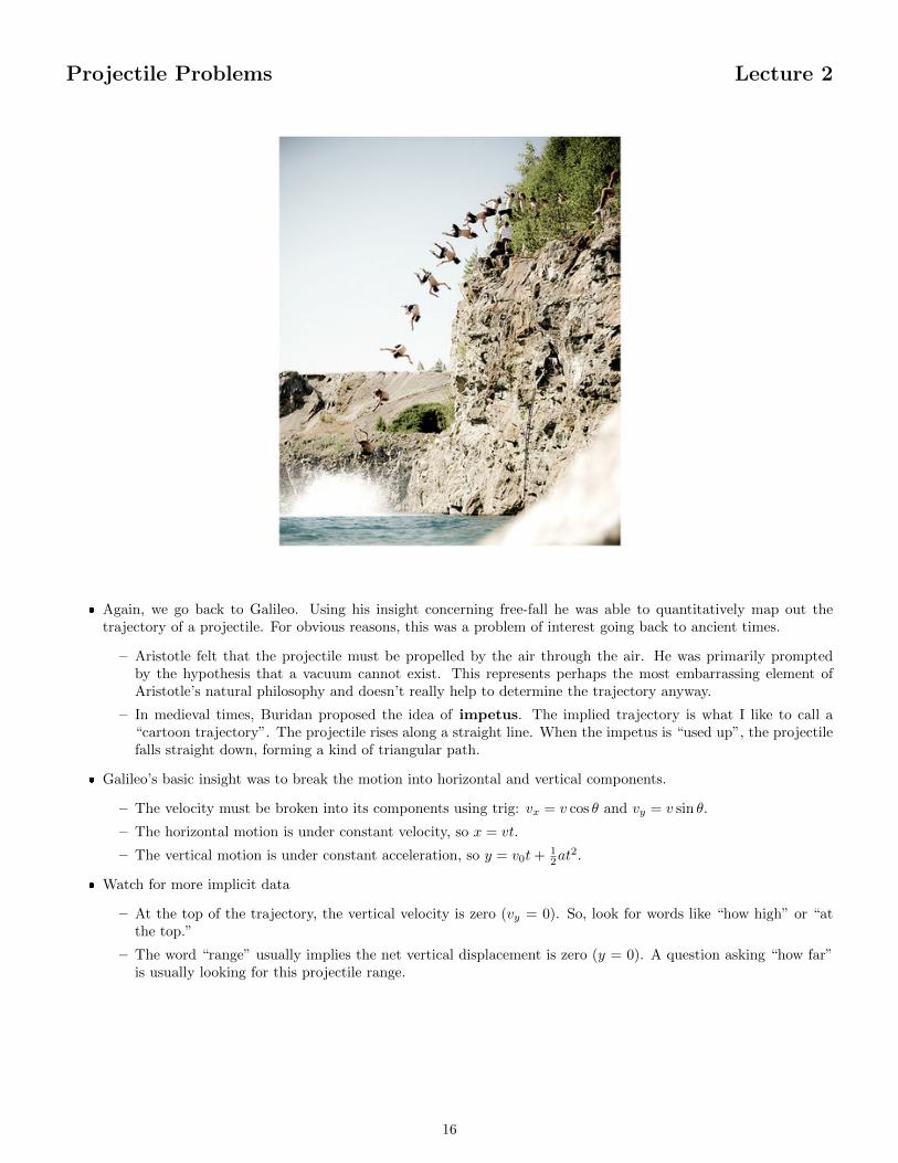
Projectile Problems Lecture 2

� Again, we go back to Galileo. Using his insight concerning free-fall he was able to quantitatively map out thetrajectory of a projectile. For obvious reasons, this was a problem of interest going back to ancient times.

– Aristotle felt that the projectile must be propelled by the air through the air. He was primarily promptedby the hypothesis that a vacuum cannot exist. This represents perhaps the most embarrassing element ofAristotle’s natural philosophy and doesn’t really help to determine the trajectory anyway.

– In medieval times, Buridan proposed the idea of impetus. The implied trajectory is what I like to call a“cartoon trajectory”. The projectile rises along a straight line. When the impetus is “used up”, the projectilefalls straight down, forming a kind of triangular path.

� Galileo’s basic insight was to break the motion into horizontal and vertical components.

– The velocity must be broken into its components using trig: vx = v cos θ and vy = v sin θ.

– The horizontal motion is under constant velocity, so x = vt.

– The vertical motion is under constant acceleration, so y = v0t+ 12at

2.

� Watch for more implicit data

– At the top of the trajectory, the vertical velocity is zero (vy = 0). So, look for words like “how high” or “atthe top.”

– The word “range” usually implies the net vertical displacement is zero (y = 0). A question asking “how far”is usually looking for this projectile range.

16

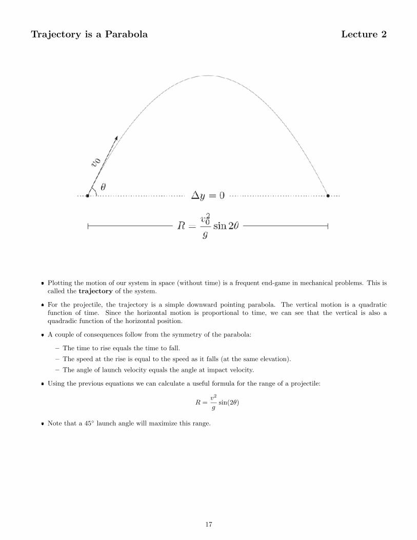
Trajectory is a Parabola Lecture 2

� Plotting the motion of our system in space (without time) is a frequent end-game in mechanical problems. This iscalled the trajectory of the system.

� For the projectile, the trajectory is a simple downward pointing parabola. The vertical motion is a quadraticfunction of time. Since the horizontal motion is proportional to time, we can see that the vertical is also aquadradic function of the horizontal position.

� A couple of consequences follow from the symmetry of the parabola:

– The time to rise equals the time to fall.

– The speed at the rise is equal to the speed as it falls (at the same elevation).

– The angle of launch velocity equals the angle at impact velocity.

� Using the previous equations we can calculate a useful formula for the range of a projectile:

R =v2

gsin(2θ)

� Note that a 45◦ launch angle will maximize this range.

17

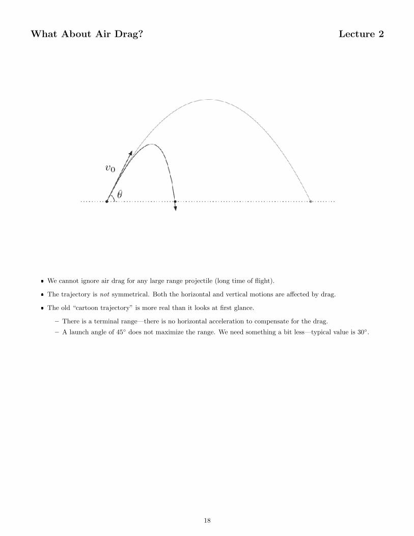
What About Air Drag? Lecture 2

� We cannot ignore air drag for any large range projectile (long time of flight).

� The trajectory is not symmetrical. Both the horizontal and vertical motions are affected by drag.

� The old “cartoon trajectory” is more real than it looks at first glance.

– There is a terminal range—there is no horizontal acceleration to compensate for the drag.

– A launch angle of 45◦ does not maximize the range. We need something a bit less—typical value is 30◦.

18

Vectors and Equilibrium Lecture 3

� Last week we spent time discussing some basic tools to analyze the motion of the simplest of all systems: theparticle.

� This week, we discuss the cause of motion, that is, force. This is wrapped up in Newton’s 2nd law of motion:F = ma.

� In this lecture we discuss the simplest of all possible motion: no motion at all!

� This occurs when all the forces balance—so we need to talk about how to calculate with these forces mathematicallyalso.

19

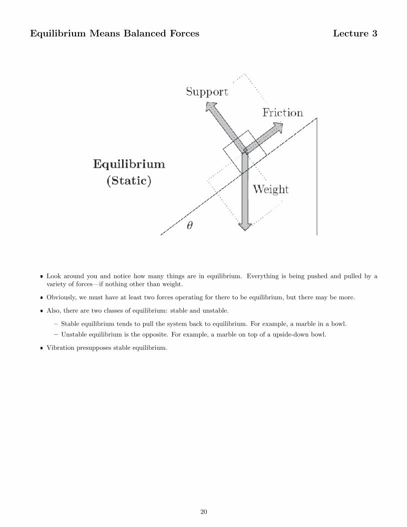
Equilibrium Means Balanced Forces Lecture 3

� Look around you and notice how many things are in equilibrium. Everything is being pushed and pulled by avariety of forces—if nothing other than weight.

� Obviously, we must have at least two forces operating for there to be equilibrium, but there may be more.

� Also, there are two classes of equilibrium: stable and unstable.

– Stable equilibrium tends to pull the system back to equilibrium. For example, a marble in a bowl.

– Unstable equilibrium is the opposite. For example, a marble on top of a upside-down bowl.

� Vibration presupposes stable equilibrium.

20

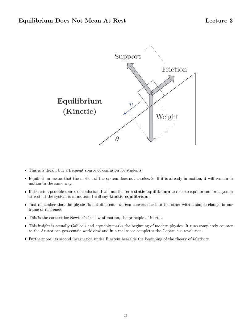
Equilibrium Does Not Mean At Rest Lecture 3

� This is a detail, but a frequent source of confusion for students.

� Equilibrium means that the motion of the system does not accelerate. If it is already in motion, it will remain inmotion in the same way.

� If there is a possible source of confusion, I will use the term static equilibrium to refer to equilibrium for a systemat rest. If the system is in motion, I will say kinetic equilibrium.

� Just remember that the physics is not different—we can convert one into the other with a simple change in ourframe of reference.

� This is the context for Newton’s 1st law of motion, the principle of inertia.

� This insight is actually Galileo’s and arguably marks the beginning of modern physics. It runs completely counterto the Aristotlean geo-centric worldview and in a real sense completes the Copernicus revolution.

� Furthermore, its second incarnation under Einstein hearalds the beginning of the theory of relativity.

21

Balance in Every Dimension Lecture 3

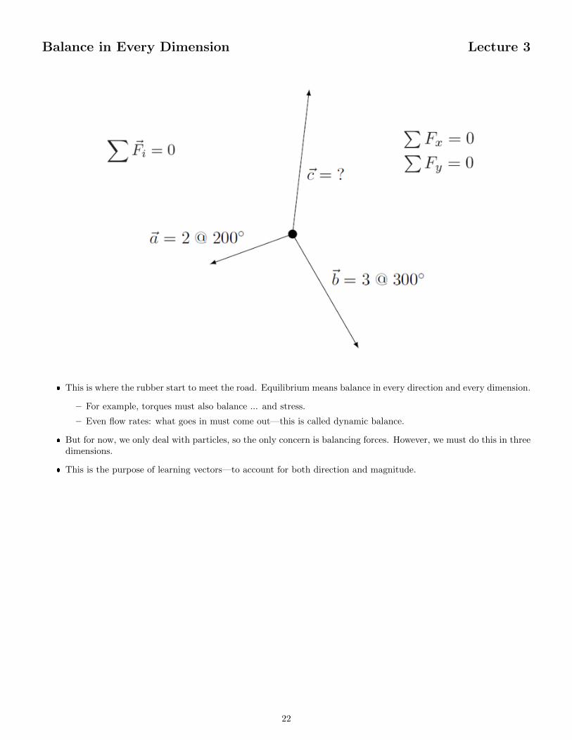
� This is where the rubber start to meet the road. Equilibrium means balance in every direction and every dimension.

– For example, torques must also balance ... and stress.

– Even flow rates: what goes in must come out—this is called dynamic balance.

� But for now, we only deal with particles, so the only concern is balancing forces. However, we must do this in threedimensions.

� This is the purpose of learning vectors—to account for both direction and magnitude.

22

Force Components Lecture 3

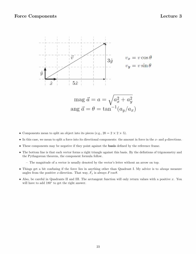
� Components mean to split an object into its pieces (e.g., 20 = 2 Ö 2 Ö 5).

� In this case, we mean to split a force into its directional components: the amount in force in the x- and y-directions.

� These components may be negative if they point against the basis defined by the reference frame.

� The bottom line is that each vector forms a right triangle against this basis. By the defintions of trigonometry andthe Pythagorean theorem, the component formula follow.

– The magnitude of a vector is usually denoted by the vector’s letter without an arrow on top.

� Things get a bit confusing if the force lies in anything other than Quadrant I. My advice is to always measureangles from the positive x-direction. That way, Fx is always F cos θ.

� Also, be careful in Quadrants II and III. The arctangent function will only return values with a positive x. Youwill have to add 180◦ to get the right answer.

23

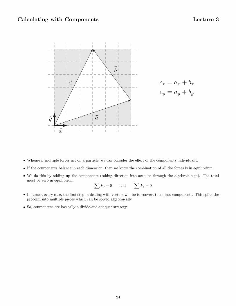
Calculating with Components Lecture 3

� Whenever multiple forces act on a particle, we can consider the effect of the components individually.

� If the components balance in each dimension, then we know the combination of all the forces is in equilibrium.

� We do this by adding up the components (taking direction into account through the algebraic sign). The totalmust be zero in equilibrium. ∑

Fx = 0 and∑

Fy = 0

� In almost every case, the first step in dealing with vectors will be to convert them into components. This splits theproblem into multiple pieces which can be solved algebraically.

� So, components are basically a divide-and-conquer strategy.

24

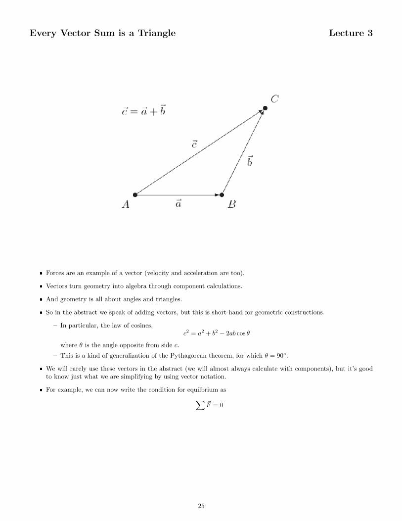
Every Vector Sum is a Triangle Lecture 3

� Forces are an example of a vector (velocity and acceleration are too).

� Vectors turn geometry into algebra through component calculations.

� And geometry is all about angles and triangles.

� So in the abstract we speak of adding vectors, but this is short-hand for geometric constructions.

– In particular, the law of cosines,c2 = a2 + b2 − 2ab cos θ

where θ is the angle opposite from side c.

– This is a kind of generalization of the Pythagorean theorem, for which θ = 90◦.

� We will rarely use these vectors in the abstract (we will almost always calculate with components), but it’s goodto know just what we are simplifying by using vector notation.

� For example, we can now write the condition for equilbrium as∑~F = 0

25

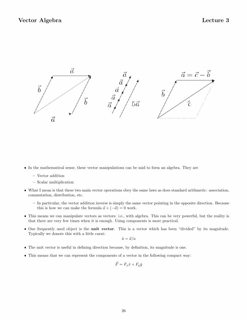
Vector Algebra Lecture 3

� In the mathematical sense, these vector manipulations can be said to form an algebra. They are

– Vector addition

– Scalar multiplication

� What I mean is that these two main vector operations obey the same laws as does standard arithmetic: association,commutation, distribution, etc.

– In particular, the vector addition inverse is simply the same vector pointing in the opposite direction. Becausethis is how we can make the formula ~a+ (−~a) = 0 work.

� This means we can manipulate vectors as vectors: i.e., with algebra. This can be very powerful, but the reality isthat there are very few times when it is enough. Using components is more practical.

� One frequently used object is the unit vector. This is a vector which has been “divided” by its magnitude.Typically we donote this with a little carat:

a = ~a/a

� The unit vector is useful in defining direction because, by definition, its magnitude is one.

� This means that we can represent the components of a vector in the following compact way:

~F = Fxx+ Fy y

26

More Vector Algebra Lecture 3

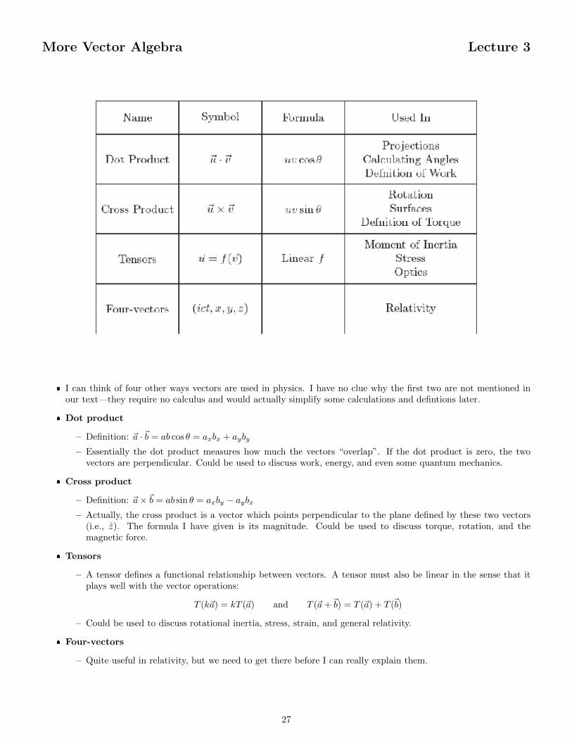
� I can think of four other ways vectors are used in physics. I have no clue why the first two are not mentioned inour text—they require no calculus and would actually simplify some calculations and defintions later.

� Dot product

– Definition: ~a ·~b = ab cos θ = axbx + ayby

– Essentially the dot product measures how much the vectors “overlap”. If the dot product is zero, the twovectors are perpendicular. Could be used to discuss work, energy, and even some quantum mechanics.

� Cross product

– Definition: ~a×~b = ab sin θ = axby − aybx– Actually, the cross product is a vector which points perpendicular to the plane defined by these two vectors

(i.e., z). The formula I have given is its magnitude. Could be used to discuss torque, rotation, and themagnetic force.

� Tensors

– A tensor defines a functional relationship between vectors. A tensor must also be linear in the sense that itplays well with the vector operations:

T (k~a) = kT (~a) and T (~a+~b) = T (~a) + T (~b)

– Could be used to discuss rotational inertia, stress, strain, and general relativity.

� Four-vectors

– Quite useful in relativity, but we need to get there before I can really explain them.

27

Force and Acceleration Lecture 4

� In this lecture we continue to discuss force and Newton’s laws of motion.

� The key is the second law, F = ma.

� For equilibrium, a = 0, so the last lecture can be seen as a subset of this one.

� We also discuss the basic mechanical forces of weight, tension, support, and friction.

� This lecture lays the foundation of classical mechanics and the rest of the course.

28

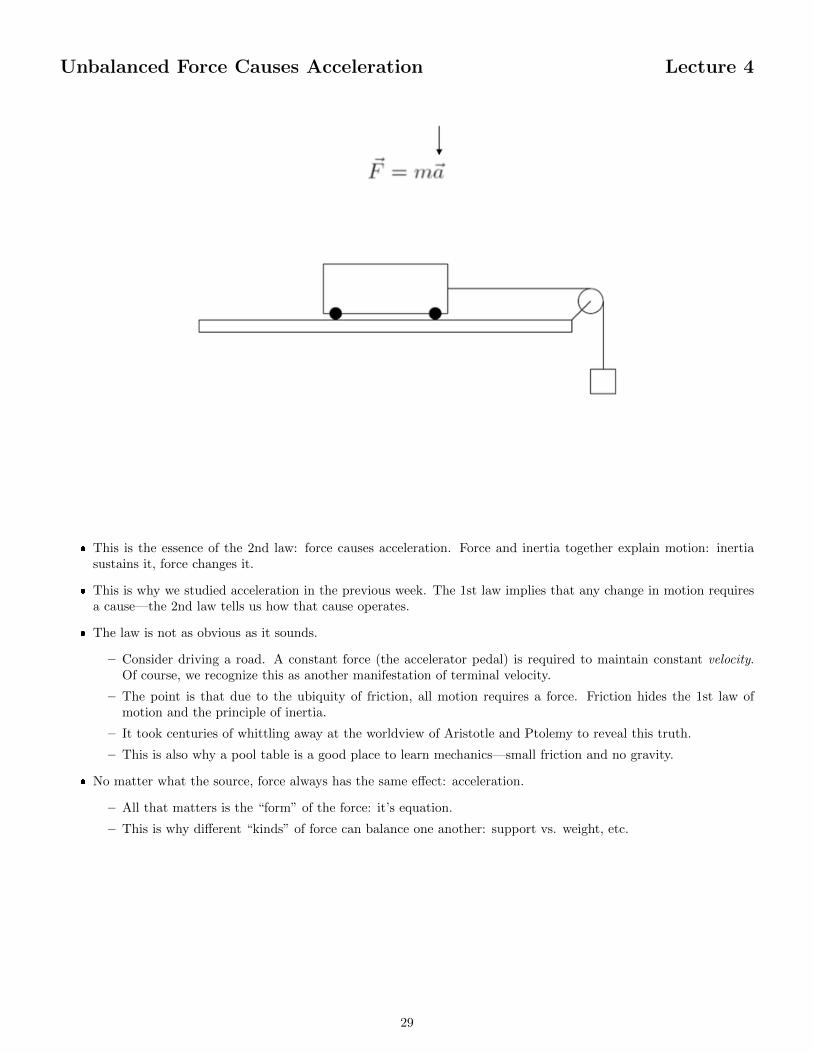
Unbalanced Force Causes Acceleration Lecture 4

� This is the essence of the 2nd law: force causes acceleration. Force and inertia together explain motion: inertiasustains it, force changes it.

� This is why we studied acceleration in the previous week. The 1st law implies that any change in motion requiresa cause—the 2nd law tells us how that cause operates.

� The law is not as obvious as it sounds.

– Consider driving a road. A constant force (the accelerator pedal) is required to maintain constant velocity.Of course, we recognize this as another manifestation of terminal velocity.

– The point is that due to the ubiquity of friction, all motion requires a force. Friction hides the 1st law ofmotion and the principle of inertia.

– It took centuries of whittling away at the worldview of Aristotle and Ptolemy to reveal this truth.

– This is also why a pool table is a good place to learn mechanics—small friction and no gravity.

� No matter what the source, force always has the same effect: acceleration.

– All that matters is the “form” of the force: it’s equation.

– This is why different “kinds” of force can balance one another: support vs. weight, etc.

29

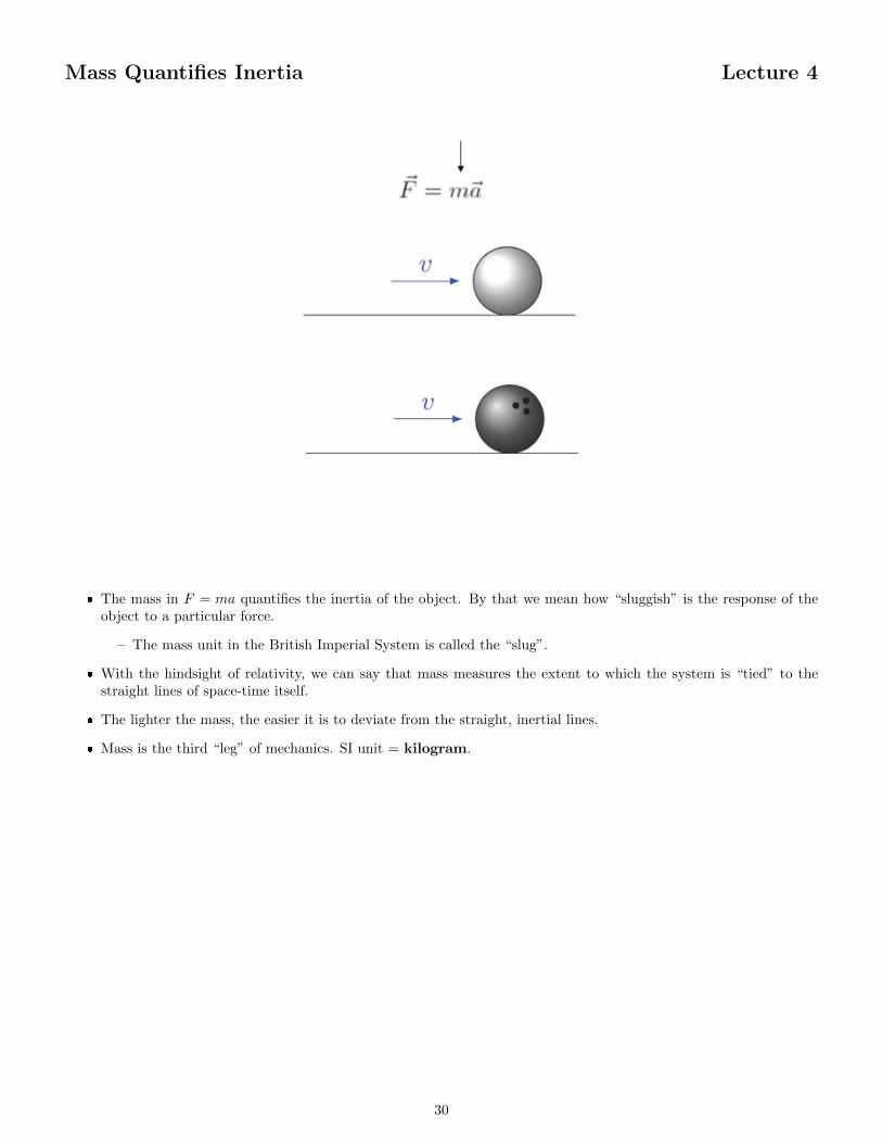
Mass Quantifies Inertia Lecture 4

� The mass in F = ma quantifies the inertia of the object. By that we mean how “sluggish” is the response of theobject to a particular force.

– The mass unit in the British Imperial System is called the “slug”.

� With the hindsight of relativity, we can say that mass measures the extent to which the system is “tied” to thestraight lines of space-time itself.

� The lighter the mass, the easier it is to deviate from the straight, inertial lines.

� Mass is the third “leg” of mechanics. SI unit = kilogram.

30

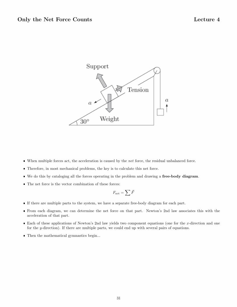
Only the Net Force Counts Lecture 4

� When multiple forces act, the acceleration is caused by the net force, the residual unbalanced force.

� Therefore, in most mechanical problems, the key is to calculate this net force.

� We do this by cataloging all the forces operating in the problem and drawing a free-body diagram.

� The net force is the vector combination of these forces:

Fnet =∑

~F

� If there are multiple parts to the system, we have a separate free-body diagram for each part.

� From each diagram, we can determine the net force on that part. Newton’s 2nd law associates this with theacceleration of that part.

� Each of these applications of Newton’s 2nd law yields two component equations (one for the x-direction and onefor the y-direction). If there are multiple parts, we could end up with several pairs of equations.

� Then the mathematical gymnastics begin...

31

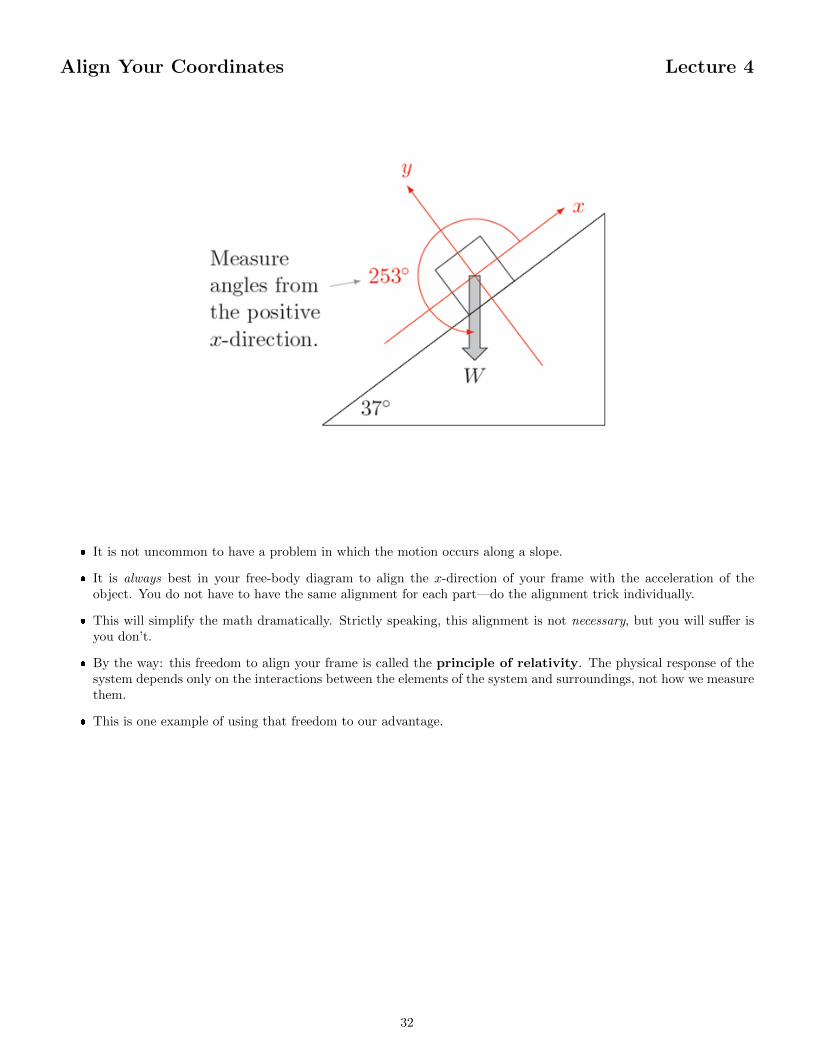
Align Your Coordinates Lecture 4

� It is not uncommon to have a problem in which the motion occurs along a slope.

� It is always best in your free-body diagram to align the x-direction of your frame with the acceleration of theobject. You do not have to have the same alignment for each part—do the alignment trick individually.

� This will simplify the math dramatically. Strictly speaking, this alignment is not necessary, but you will suffer isyou don’t.

� By the way: this freedom to align your frame is called the principle of relativity. The physical response of thesystem depends only on the interactions between the elements of the system and surroundings, not how we measurethem.

� This is one example of using that freedom to our advantage.

32

Weight, Tension, Strings, and Pulleys Lecture 4

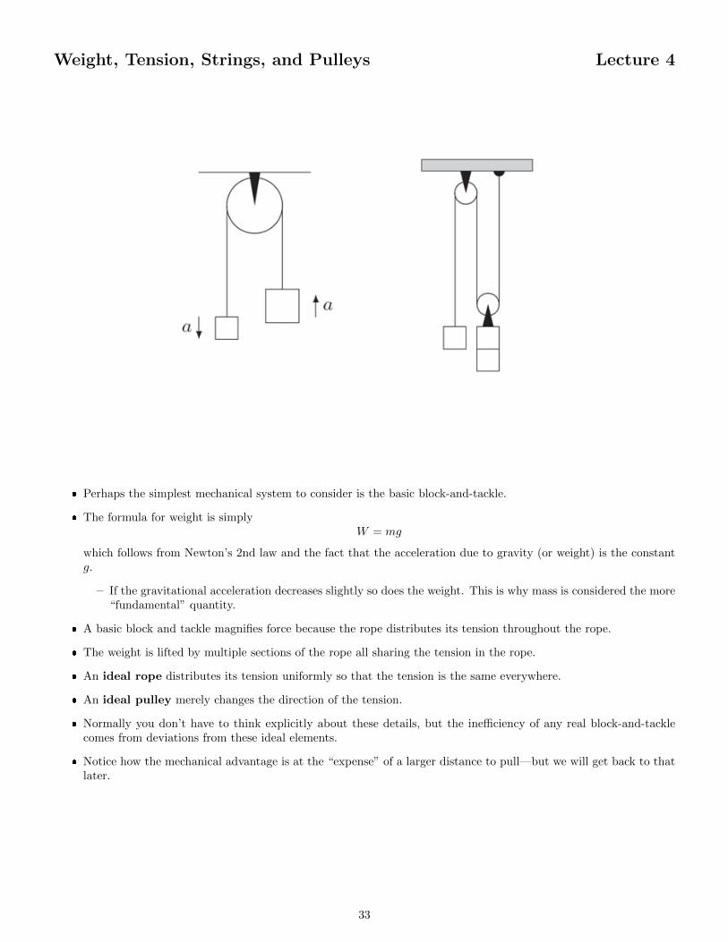
� Perhaps the simplest mechanical system to consider is the basic block-and-tackle.

� The formula for weight is simplyW = mg

which follows from Newton’s 2nd law and the fact that the acceleration due to gravity (or weight) is the constantg.

– If the gravitational acceleration decreases slightly so does the weight. This is why mass is considered the more“fundamental” quantity.

� A basic block and tackle magnifies force because the rope distributes its tension throughout the rope.

� The weight is lifted by multiple sections of the rope all sharing the tension in the rope.

� An ideal rope distributes its tension uniformly so that the tension is the same everywhere.

� An ideal pulley merely changes the direction of the tension.

� Normally you don’t have to think explicitly about these details, but the inefficiency of any real block-and-tacklecomes from deviations from these ideal elements.

� Notice how the mechanical advantage is at the “expense” of a larger distance to pull—but we will get back to thatlater.

33

Support and Elastic Forces Lecture 4

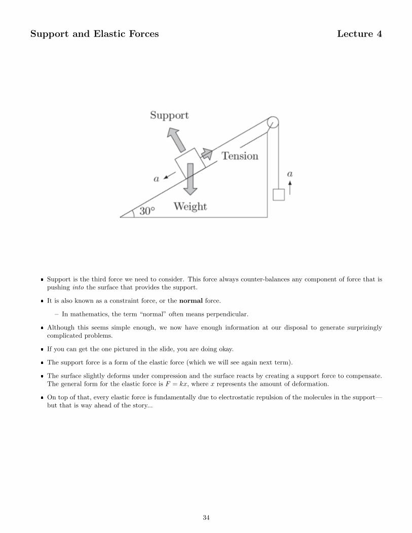
� Support is the third force we need to consider. This force always counter-balances any component of force that ispushing into the surface that provides the support.

� It is also known as a constraint force, or the normal force.

– In mathematics, the term “normal” often means perpendicular.

� Although this seems simple enough, we now have enough information at our disposal to generate surprizinglycomplicated problems.

� If you can get the one pictured in the slide, you are doing okay.

� The support force is a form of the elastic force (which we will see again next term).

� The surface slightly deforms under compression and the surface reacts by creating a support force to compensate.The general form for the elastic force is F = kx, where x represents the amount of deformation.

� On top of that, every elastic force is fundamentally due to electrostatic repulsion of the molecules in the support—but that is way ahead of the story...

34

Friction: Kinetic and Static Lecture 4

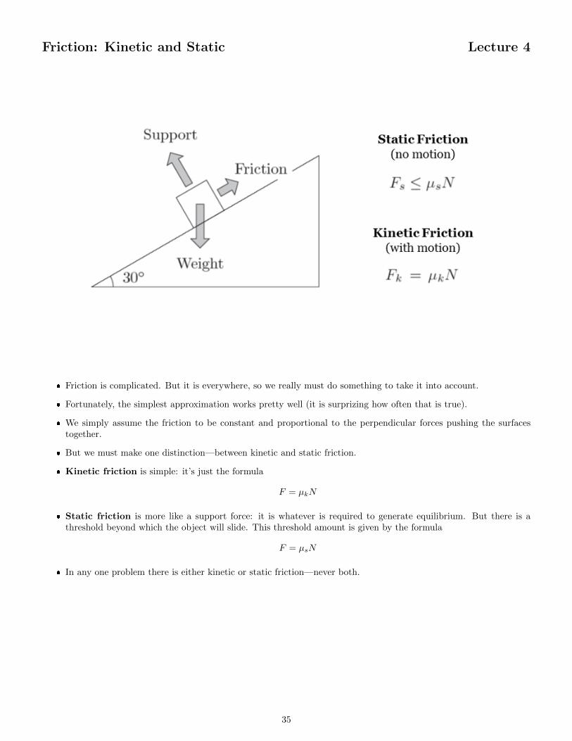
� Friction is complicated. But it is everywhere, so we really must do something to take it into account.

� Fortunately, the simplest approximation works pretty well (it is surprizing how often that is true).

� We simply assume the friction to be constant and proportional to the perpendicular forces pushing the surfacestogether.

� But we must make one distinction—between kinetic and static friction.

� Kinetic friction is simple: it’s just the formula

F = µkN

� Static friction is more like a support force: it is whatever is required to generate equilibrium. But there is athreshold beyond which the object will slide. This threshold amount is given by the formula

F = µsN

� In any one problem there is either kinetic or static friction—never both.

35

The Long-Range Forces Lecture 4

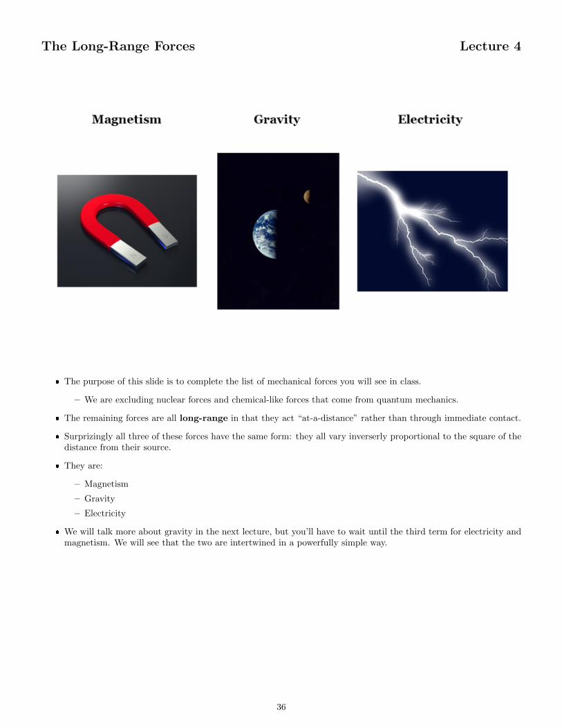
� The purpose of this slide is to complete the list of mechanical forces you will see in class.

– We are excluding nuclear forces and chemical-like forces that come from quantum mechanics.

� The remaining forces are all long-range in that they act “at-a-distance” rather than through immediate contact.

� Surprizingly all three of these forces have the same form: they all vary inverserly proportional to the square of thedistance from their source.

� They are:

– Magnetism

– Gravity

– Electricity

� We will talk more about gravity in the next lecture, but you’ll have to wait until the third term for electricity andmagnetism. We will see that the two are intertwined in a powerfully simple way.

36

Circular Motion and Gravity Lecture 5

� Today we talk about circular motion. There are two reasons to do this...

� Last week we talked about Newton’s laws in problems dealing with straight-line motion. Circular motion providesa prototype for motion that is deflected instead.

� Secondly, circular motion has historically been associated with the sky. One of Newton’s most dramatic triumphswas showing how the laws of motion can be applied to celestial motion.

� This was one of the great “unification” moments in physics history.

� And this is why I feel it more appropriate to discuss Newton’s law of gravity in this lecture rather than the previousone.

37

Acceleration for Uniform Circular Motion Lecture 5

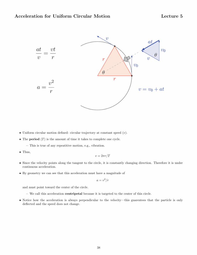
� Uniform circular motion defined: circular trajectory at constant speed (v).

� The period (T ) is the amount of time it takes to complete one cycle.

– This is true of any repeatitive motion, e.g., vibration.

� Thus,v = 2πr/T

� Since the velocity points along the tangent to the circle, it is constantly changing direction. Therefore it is undercontinuous acceleration.

� By geometry we can see that this acceleration must have a magnitude of

a = v2/r

and must point toward the center of the circle.

– We call this acceleration centripetal because it is targeted to the center of this circle.

� Notice how the acceleration is always perpendicular to the velocity—this guarentees that the particle is onlydeflected and the speed does not change.

38

Centripetal Force is the Net Force Lecture 5

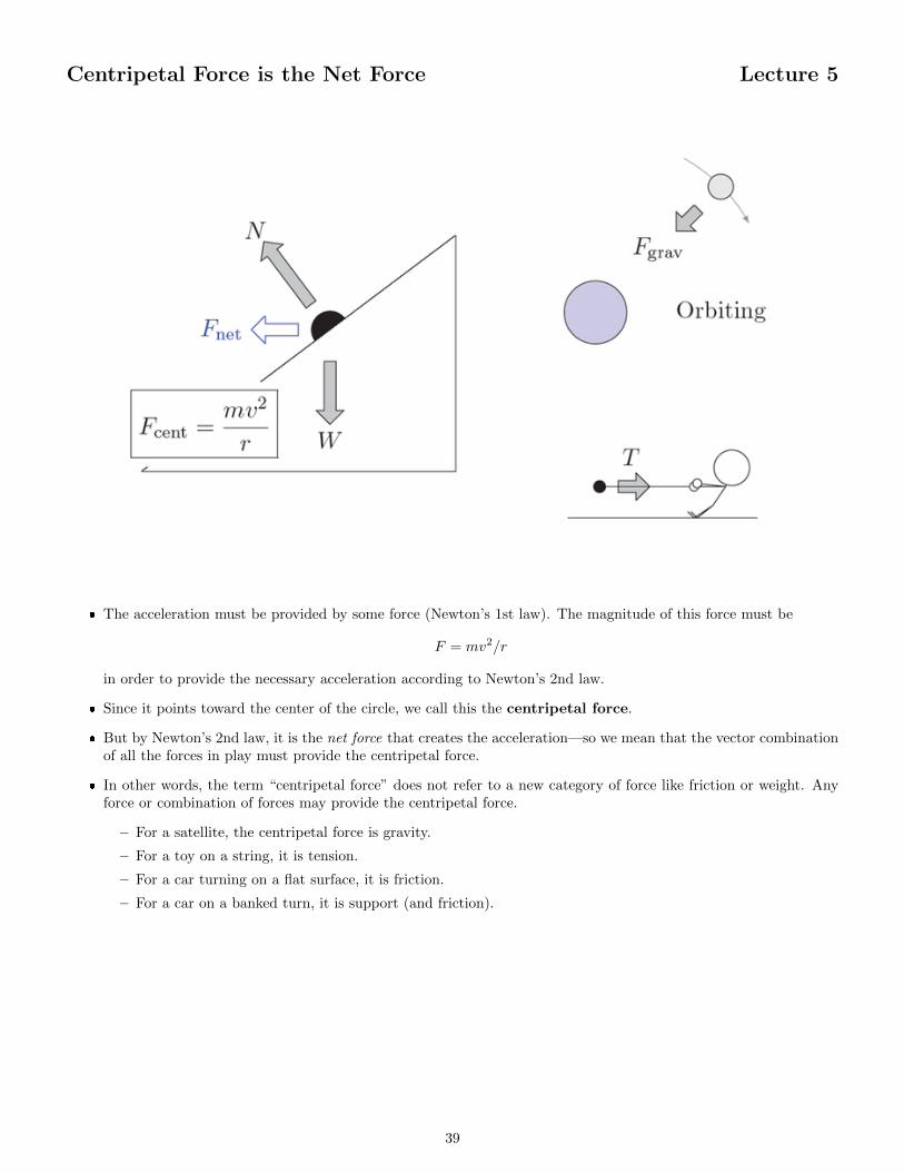
� The acceleration must be provided by some force (Newton’s 1st law). The magnitude of this force must be

F = mv2/r

in order to provide the necessary acceleration according to Newton’s 2nd law.

� Since it points toward the center of the circle, we call this the centripetal force.

� But by Newton’s 2nd law, it is the net force that creates the acceleration—so we mean that the vector combinationof all the forces in play must provide the centripetal force.

� In other words, the term “centripetal force” does not refer to a new category of force like friction or weight. Anyforce or combination of forces may provide the centripetal force.

– For a satellite, the centripetal force is gravity.

– For a toy on a string, it is tension.

– For a car turning on a flat surface, it is friction.

– For a car on a banked turn, it is support (and friction).

39

Radius of Curvature Lecture 5

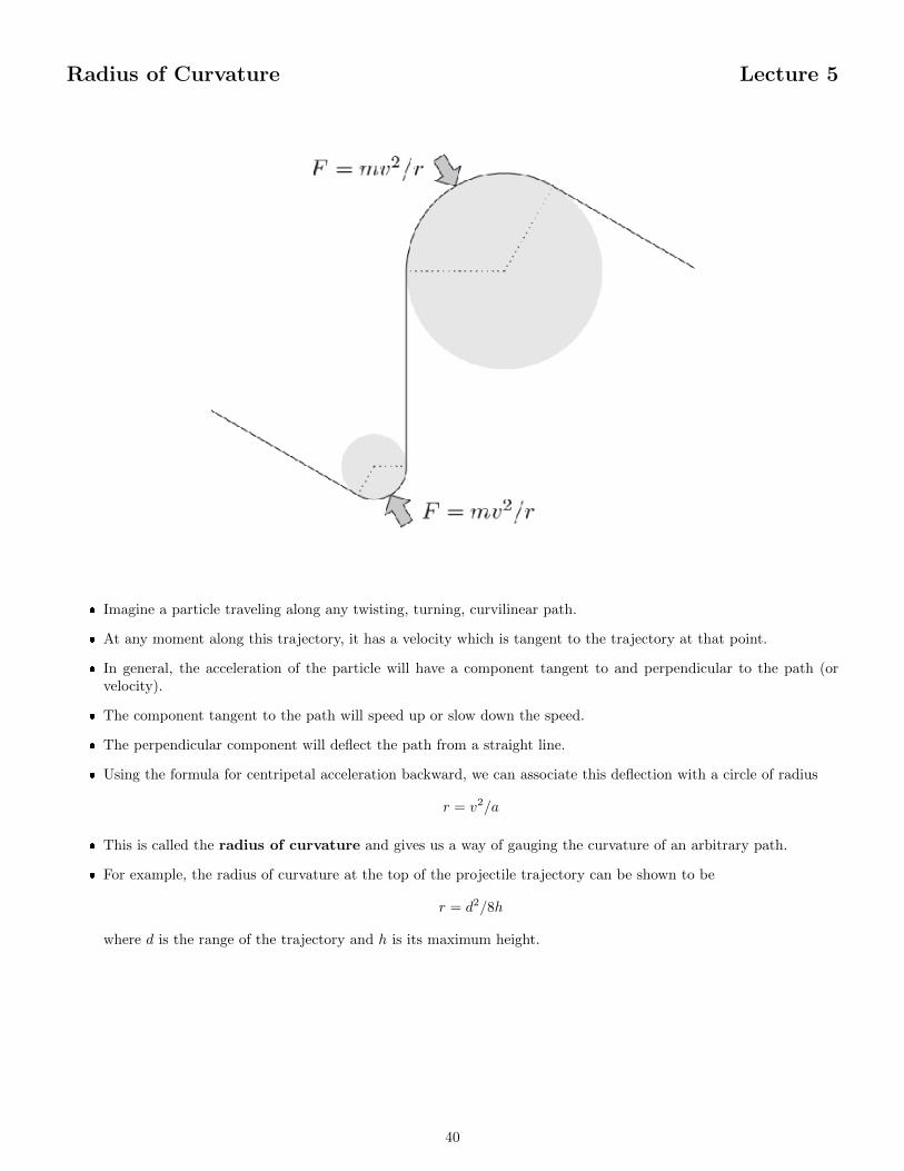
� Imagine a particle traveling along any twisting, turning, curvilinear path.

� At any moment along this trajectory, it has a velocity which is tangent to the trajectory at that point.

� In general, the acceleration of the particle will have a component tangent to and perpendicular to the path (orvelocity).

� The component tangent to the path will speed up or slow down the speed.

� The perpendicular component will deflect the path from a straight line.

� Using the formula for centripetal acceleration backward, we can associate this deflection with a circle of radius

r = v2/a

� This is called the radius of curvature and gives us a way of gauging the curvature of an arbitrary path.

� For example, the radius of curvature at the top of the projectile trajectory can be shown to be

r = d2/8h

where d is the range of the trajectory and h is its maximum height.

40

Rotating Frames and Inertial Forces Lecture 5

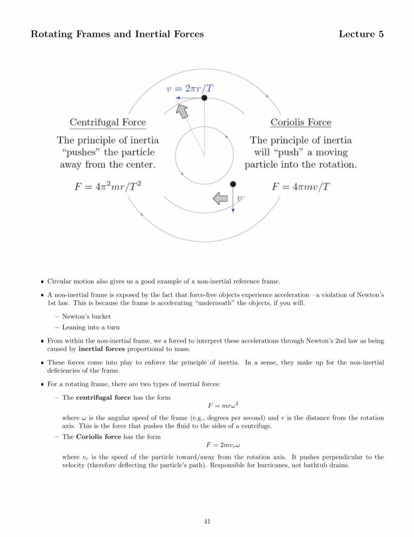
� Circular motion also gives us a good example of a non-inertial reference frame.

� A non-inertial frame is exposed by the fact that force-free objects experience acceleration—a violation of Newton’s1st law. This is because the frame is accelerating “underneath” the objects, if you will.

– Newton’s bucket

– Leaning into a turn

� From within the non-inertial frame, we a forced to interpret these accelerations through Newton’s 2nd law as beingcaused by inertial forces proportional to mass.

� These forces come into play to enforce the principle of inertia. In a sense, they make up for the non-inertialdeficiencies of the frame.

� For a rotating frame, there are two types of inertial forces:

– The centrifugal force has the formF = mrω2

where ω is the angular speed of the frame (e.g., degrees per second) and r is the distance from the rotationaxis. This is the force that pushes the fluid to the sides of a centrifuge.

– The Coriolis force has the formF = 2mvrω

where vr is the speed of the particle toward/away from the rotation axis. It pushes perpendicular to thevelocity (therefore deflecting the particle’s path). Responsible for hurricanes, not bathtub drains.

41

Newton’s Law of Gravity Lecture 5

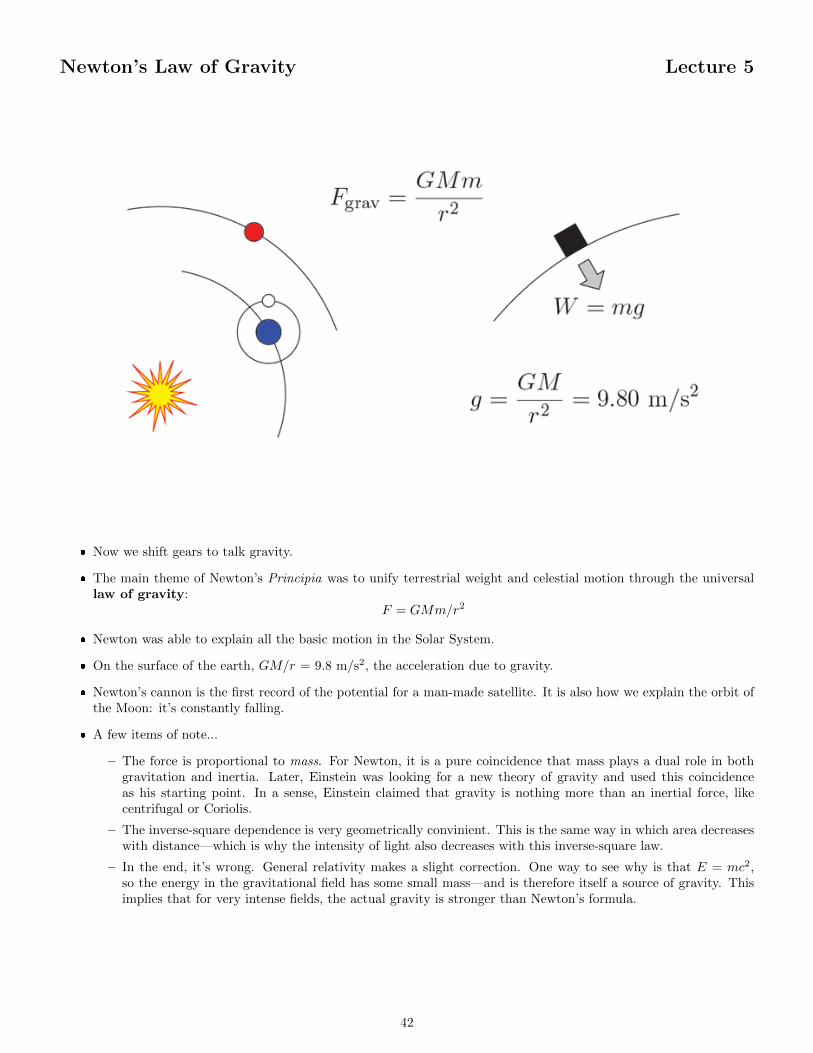
� Now we shift gears to talk gravity.

� The main theme of Newton’s Principia was to unify terrestrial weight and celestial motion through the universallaw of gravity:

F = GMm/r2

� Newton was able to explain all the basic motion in the Solar System.

� On the surface of the earth, GM/r = 9.8 m/s2, the acceleration due to gravity.

� Newton’s cannon is the first record of the potential for a man-made satellite. It is also how we explain the orbit ofthe Moon: it’s constantly falling.

� A few items of note...

– The force is proportional to mass. For Newton, it is a pure coincidence that mass plays a dual role in bothgravitation and inertia. Later, Einstein was looking for a new theory of gravity and used this coincidenceas his starting point. In a sense, Einstein claimed that gravity is nothing more than an inertial force, likecentrifugal or Coriolis.

– The inverse-square dependence is very geometrically convinient. This is the same way in which area decreaseswith distance—which is why the intensity of light also decreases with this inverse-square law.

– In the end, it’s wrong. General relativity makes a slight correction. One way to see why is that E = mc2,so the energy in the gravitational field has some small mass—and is therefore itself a source of gravity. Thisimplies that for very intense fields, the actual gravity is stronger than Newton’s formula.

42

Kepler’s Third Law Lecture 5

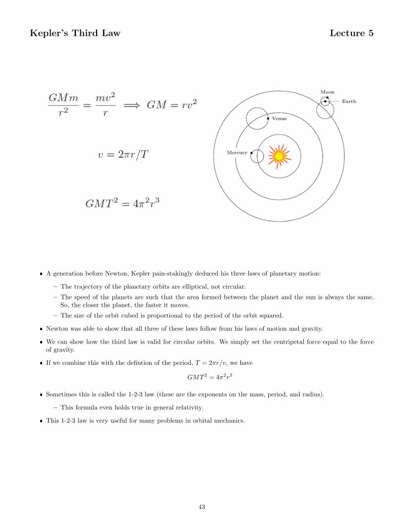
� A generation before Newton, Kepler pain-stakingly deduced his three laws of planetary motion:

– The trajectory of the planetary orbits are elliptical, not circular.

– The speed of the planets are such that the area formed between the planet and the sun is always the same.So, the closer the planet, the faster it moves.

– The size of the orbit cubed is proportional to the period of the orbit squared.

� Newton was able to show that all three of these laws follow from his laws of motion and gravity.

� We can show how the third law is valid for circular orbits. We simply set the centripetal force equal to the forceof gravity.

� If we combine this with the defintion of the period, T = 2πr/v, we have

GMT 2 = 4π2r3

� Sometimes this is called the 1-2-3 law (these are the exponents on the mass, period, and radius).

– This formula even holds true in general relativity.

� This 1-2-3 law is very useful for many problems in orbital mechanics.

43

From Kepler: Saturn’s Rings, Dark Matter Lecture 5

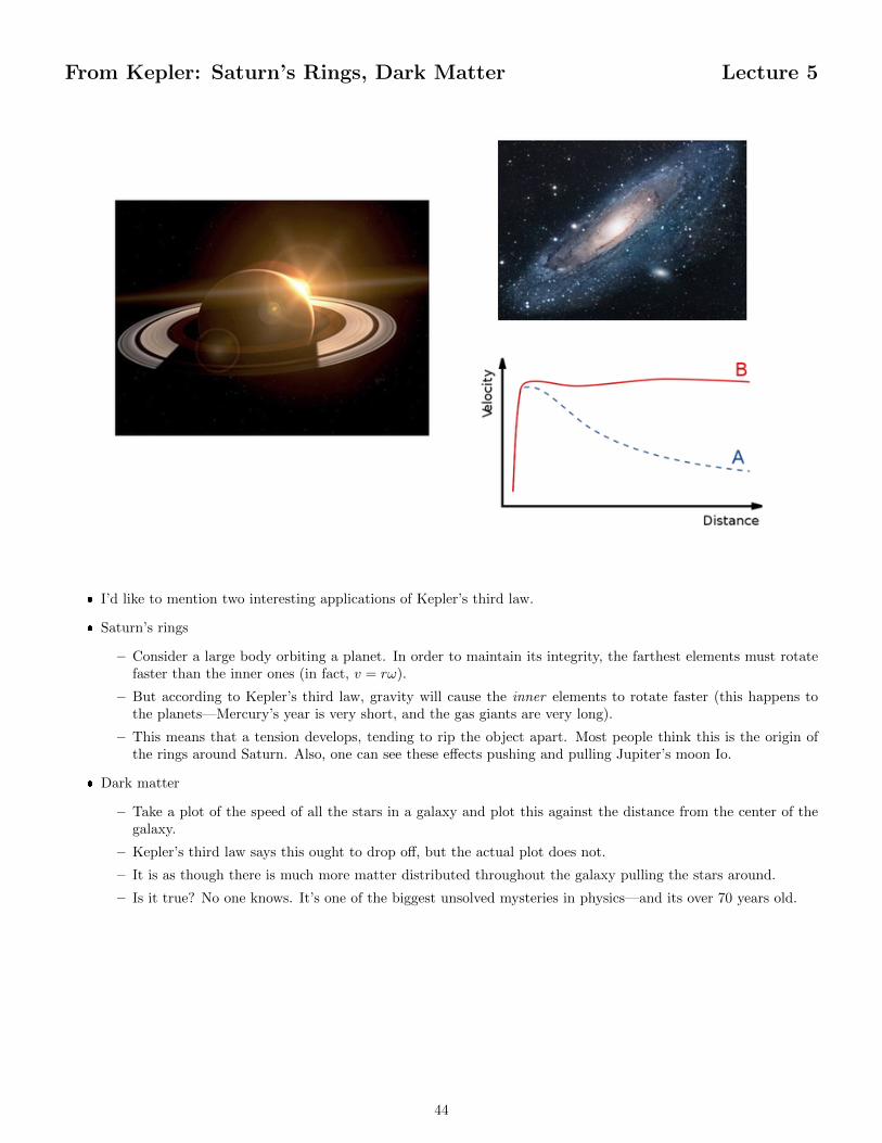
� I’d like to mention two interesting applications of Kepler’s third law.

� Saturn’s rings

– Consider a large body orbiting a planet. In order to maintain its integrity, the farthest elements must rotatefaster than the inner ones (in fact, v = rω).

– But according to Kepler’s third law, gravity will cause the inner elements to rotate faster (this happens tothe planets—Mercury’s year is very short, and the gas giants are very long).

– This means that a tension develops, tending to rip the object apart. Most people think this is the origin ofthe rings around Saturn. Also, one can see these effects pushing and pulling Jupiter’s moon Io.

� Dark matter

– Take a plot of the speed of all the stars in a galaxy and plot this against the distance from the center of thegalaxy.

– Kepler’s third law says this ought to drop off, but the actual plot does not.

– It is as though there is much more matter distributed throughout the galaxy pulling the stars around.

– Is it true? No one knows. It’s one of the biggest unsolved mysteries in physics—and its over 70 years old.

44

Perturbation Corrects Kepler Lecture 5

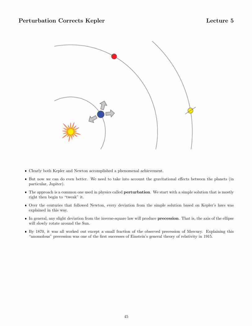
� Clearly both Kepler and Newton accomplished a phenomenal achievement.

� But now we can do even better. We need to take into account the gravitational effects between the planets (inparticular, Jupiter).

� The approach is a common one used in physics called perturbation. We start with a simple solution that is mostlyright then begin to “tweak” it.

� Over the centuries that followed Newton, every deviation from the simple solution based on Kepler’s laws wasexplained in this way.

� In general, any slight deviation from the inverse-square law will produce precession. That is, the axis of the ellipsewill slowly rotate around the Sun.

� By 1870, it was all worked out except a small fraction of the observed precession of Mercury. Explaining this“anomolous” precession was one of the first successes of Einstein’s general theory of relativity in 1915.

45

Torque and Rotation Lecture 6

� In this lecture we finally move beyond a simple particle in our mechanical analysis of motion.

� Now we consider the so-called rigid body. Essentially, a particle with extension—we still ignore the deformationpotentially caused by forces on an object.

� The new type of motion to consider is rotation. Fortunately, we will discover a close analogy exists between rotationand translation. We will use this to our advantage as we proceed.

� After this lecture we will be able to discuss most every mechanical machine or contraption—at least to a firstapproximation.

46

Two Ways to Calculate Torque Lecture 6

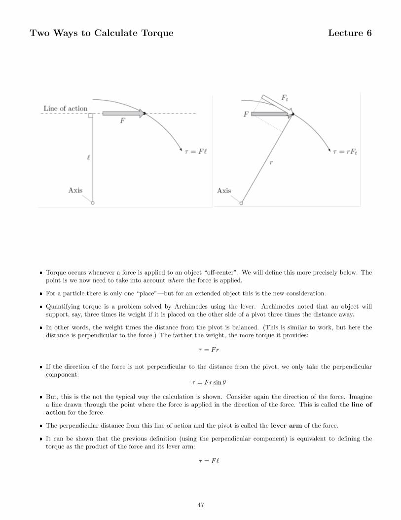
� Torque occurs whenever a force is applied to an object “off-center”. We will define this more precisely below. Thepoint is we now need to take into account where the force is applied.

� For a particle there is only one “place”—but for an extended object this is the new consideration.

� Quantifying torque is a problem solved by Archimedes using the lever. Archimedes noted that an object willsupport, say, three times its weight if it is placed on the other side of a pivot three times the distance away.

� In other words, the weight times the distance from the pivot is balanced. (This is similar to work, but here thedistance is perpendicular to the force.) The farther the weight, the more torque it provides:

τ = Fr

� If the direction of the force is not perpendicular to the distance from the pivot, we only take the perpendicularcomponent:

τ = Fr sin θ

� But, this is the not the typical way the calculation is shown. Consider again the direction of the force. Imaginea line drawn through the point where the force is applied in the direction of the force. This is called the line ofaction for the force.

� The perpendicular distance from this line of action and the pivot is called the lever arm of the force.

� It can be shown that the previous definition (using the perpendicular component) is equivalent to defining thetorque as the product of the force and its lever arm:

τ = F`

47

Static Equilibrium, Again Lecture 6

� Using the idea of torque, we can now analyze static equilibrium problems with extended objects.

� Remember that equilibrium implies balance in all directions and dimensions. For us that means we now mustbalance the torques.

� We have three main equations to use in any static equilibrium problem:∑Fx = 0 and

∑Fy = 0 and

∑τ = 0

� One thing to note on the torque equation is your signs. If you measure all the angles in the same way, your signsreally ought to come out right, but...

� Frequently, calculating the torques in these problems is the hardest part. The geometry and trig can be quiteconfusing. I frequently simply determine the magnitude of the torque and then append the sign at the end.

� A positive torque will tend to rotate the system counter-clockwise. So if the force is to the right of the pivot andpointing up, that is positive. If the force is above and pointing left, that is also positive. And so on.

� There is one other thing: where is the pivot? We need a pivot in order to calculate these torques.

� The answer is: anywhere. The torques must balance around any pivot point—if they didn’t, the system wouldrotate there.

� We can use this fact to our advantage. If we choose a point where some force is applied, the lever arm of that forceis (by definition) zero. Its torque is zero around that pivot, and if falls out of the torque calculation. You can usethis to eliminate calculating with the force you know the least about.

48

Kinematics of Rotation Lecture 6

� So much for static problems. What if the torque does not balance? Well, we know that Newton’s 2nd law mustapply and we know that this must result in rotation—but how much?

� The first thing we need to do is talk about rotation itself for a bit. Rotation is the change in orientation of anobject. We define the orientation of an object with an angle—relative to some fixed direction, usually the positivex-axis.

� As a system rotates from one orientation to another, we define its angular displacement as the difference betweenthe two. We also define its angular velocity as the rate at which this orientation changes. In symbols:

ω(t) = lim∆t→0

∆θ

∆t

� We can use degrees to measure angle, but it will be simpler to use radians. The radian is defined such that onerevolution is equal to 2π radians. This is makes the formula

s = rθ

where s is the arc-length defined by the angle on a circle with radius r.

� We also define angular acceleration as

α(t) = lim∆t→0

∆ω

∆t

� Every formula from constant accleration translates into rotation because of the parallels in these definitions:

x→ θ and v → ω and a→ α

49

Moment of Inertia Lecture 6

� Consider, for a moment, a particle constrained to rotate around some pivot (maybe its connected by a thin metalrod, or something).

� If we apply a force to this particle, it will accelerate according to Newton’s 2nd law.

� But the constraint will counter-balance the component away from or toward the pivot. Only the component tangentto rotation will drive rotation.

� If we multiply both sides of Newton’s 2nd law with r (the distance to the pivot), we get

Ftr = mv2α

because a = rα.

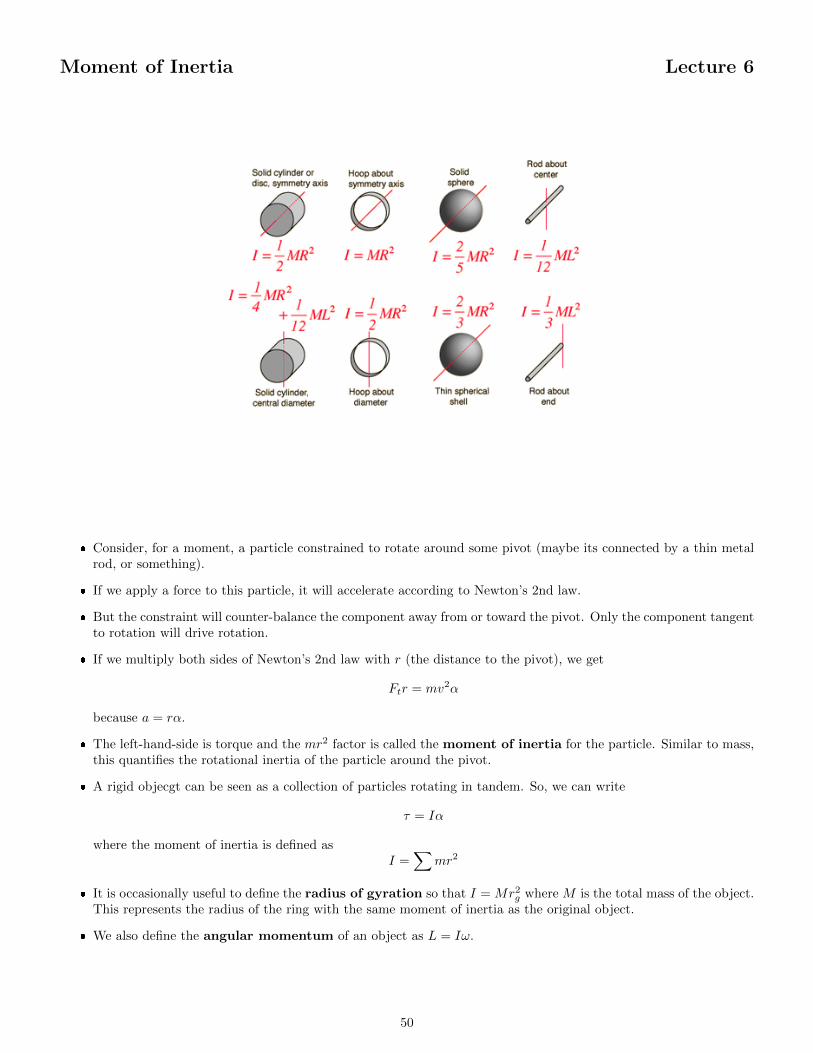
� The left-hand-side is torque and the mr2 factor is called the moment of inertia for the particle. Similar to mass,this quantifies the rotational inertia of the particle around the pivot.

� A rigid objecgt can be seen as a collection of particles rotating in tandem. So, we can write

τ = Iα

where the moment of inertia is defined asI =

∑mr2

� It is occasionally useful to define the radius of gyration so that I = Mr2g where M is the total mass of the object.

This represents the radius of the ring with the same moment of inertia as the original object.

� We also define the angular momentum of an object as L = Iω.

50

Mechanical Analogies Lecture 6

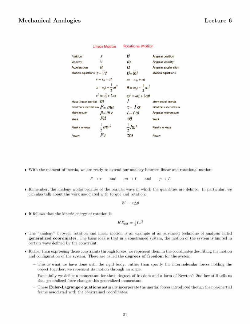
� With the moment of inertia, we are ready to extend our analogy between linear and rotational motion:

F → τ and m→ I and p→ L

� Remember, the analogy works because of the parallel ways in which the quantities are defined. In particular, wecan also talk about the work associated with torque and rotation:

W = τ∆θ

� It follows that the kinetic energy of rotation is

KErot = 12Iω

2

� The “analogy” between rotation and linear motion is an example of an advanced technique of analysis calledgeneralized coordinates. The basic idea is that in a constrained system, the motion of the system is limited incertain ways defined by the constraint.

� Rather than expressing those constraints through forces, we represent them in the coordinates describing the motionand configuration of the system. These are called the degrees of freedom for the system.

– This is what we have done with the rigid body: rather than specify the intermolecular forces holding theobject together, we represent its motion through an angle.

– Essentially we define a momentum for these degrees of freedom and a form of Newton’s 2nd law still tells usthat generalized force changes this generalized momentum.

– These Euler-Lagrange equations naturally incorporate the inertial forces introduced though the non-inertialframe associated with the constrained coordinates.

51

Rolling Things Lecture 6

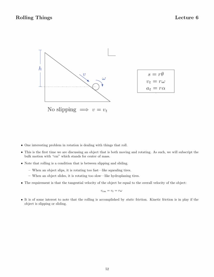
� One interesting problem in rotation is dealing with things that roll.

� This is the first time we are discussing an object that is both moving and rotating. As such, we will subscript thebulk motion with “cm” which stands for center of mass.

� Note that rolling is a condition that is between slipping and sliding.

– When an object slips, it is rotating too fast—like squealing tires.

– When an object slides, it is rotating too slow—like hydroplaning tires.

� The requirement is that the tangential velocity of the object be equal to the overall velocity of the object:

vcm = vt = rω

� It is of some interest to note that the rolling is accomplished by static friction. Kinetic friction is in play if theobject is slipping or sliding.

52

Principal Axes and Free Rotation Lecture 6

� Until now we have discussed only fixed rotation. This is when the axis of rotation is fixed in orientation. Freerotation is when the object rotates in any old way.

� In general as an object moves it rotates with a wobble. In order to understand this, we will need to refine ourdescription of rotation.

� Since each rotation involves a magnitude (the angular speed) and a direction (the axis of rotation), it makes senseto associate it with a vector.

– For fixed rotation in a plane, this vector points out of the plane.

– In addition, we can associate angular acceleration, torque, and angular momentum with vectors.

� How then do we explain the wobble?

� It happens that, for any shape object, there are certain principal axes about which the object will rotate withoutthis wobble. In this case the angular velocity vectors and the angular momentum vectors are aligned.

� For rotation off of these axes, the two are not aligned. The distribution of the mass throws off the balance of therotation.

� For an object with an axis of rotational symmetry, this axis will always be one of the principal axes.

53

More Free Rotation Lecture 6

� A rotating tire will not wobble because its principal axis is aligned with the axle. But if the axle is bent, theangular momentum is not aligned with the rotation.

� The distribution of the object’s mass is captured in the moment of inertia, and the angular momentum capturesboth the rotation and this distribution.

– This is why one will sometimes see the moment of inertia mentioned as a tensor: it is the thing that connectstwo vectors. It converts the angular velocity into the angular momentum. For fixed rotation it is enough toconsider this as a simple scalar multiplication. But for the complications associated with free rotation we needthe full power of tensors to describe the dynamics.

– Sometimes a bent axle can be fixed by adding weights to change the distribution of mass on the wheel. Thisproblem is called dynamic balancing.

� The rotation must torque the angular momentum vector around the angular velocity. These extra torques are whatcause the jarring vibrations associated with a bent axle—or the wobble in free rotation. This twirling of the axisof rotation is called gyroscopic precession.

� So far we have talked about free rotation without any external forces. If an external force is present it can causenutation which is a slight vibration in the precession of the rotating object.

� The rotation of the earth exhibits both precession and nutation.

– The earth is not quite spherical (bulges out at the equator) which causes a precession of its rotation—thismeans that the north pole is slowing moving away from the north star.

– The precession has a period of is 26,000 years and was large enough to be noticed by the ancient astronomers.The nutation in the earth’s rotation is much smaller in magnitude. The largest contribution is from the moon’sgravitation and has a period of about 18.6 years.

54

Torque and Rotation Lecture 7

� In this lecture we finally move beyond a simple particle in our mechanical analysis of motion.

� Now we consider the so-called rigid body. Essentially, a particle with extension—we still ignore the deformationpotentially caused by forces on an object.

� The new type of motion to consider is rotation. Fortunately, we will discover a close analogy exists between rotationand translation. We will use this to our advantage as we proceed.

� After this lecture we will be able to discuss most every mechanical machine or contraption—at least to a firstapproximation.

55

Two Ways to Calculate Torque Lecture 7

� Torque occurs whenever a force is applied to an object “off-center”. We will define this more precisely below. Thepoint is we now need to take into account where the force is applied.

� For a particle there is only one “place”—but for an extended object this is the new consideration.

� Quantifying torque is a problem solved by Archimedes using the lever. Archimedes noted that an object willsupport, say, three times its weight if it is placed on the other side of a pivot three times the distance away.

� In other words, the weight times the distance from the pivot is balanced. (This is similar to work, but here thedistance is perpendicular to the force.) The farther the weight, the more torque it provides:

τ = Fr

� If the direction of the force is not perpendicular to the distance from the pivot, we only take the perpendicularcomponent:

τ = Fr sin θ

� But, this is the not the typical way the calculation is shown. Consider again the direction of the force. Imaginea line drawn through the point where the force is applied in the direction of the force. This is called the line ofaction for the force.

� The perpendicular distance from this line of action and the pivot is called the lever arm of the force.

� It can be shown that the previous definition (using the perpendicular component) is equivalent to defining thetorque as the product of the force and its lever arm:

τ = F`

56

Static Equilibrium, Again Lecture 7

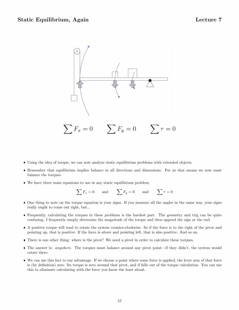
� Using the idea of torque, we can now analyze static equilibrium problems with extended objects.

� Remember that equilibrium implies balance in all directions and dimensions. For us that means we now mustbalance the torques.

� We have three main equations to use in any static equilibrium problem:∑Fx = 0 and

∑Fy = 0 and

∑τ = 0

� One thing to note on the torque equation is your signs. If you measure all the angles in the same way, your signsreally ought to come out right, but...

� Frequently, calculating the torques in these problems is the hardest part. The geometry and trig can be quiteconfusing. I frequently simply determine the magnitude of the torque and then append the sign at the end.

� A positive torque will tend to rotate the system counter-clockwise. So if the force is to the right of the pivot andpointing up, that is positive. If the force is above and pointing left, that is also positive. And so on.

� There is one other thing: where is the pivot? We need a pivot in order to calculate these torques.

� The answer is: anywhere. The torques must balance around any pivot point—if they didn’t, the system wouldrotate there.

� We can use this fact to our advantage. If we choose a point where some force is applied, the lever arm of that forceis (by definition) zero. Its torque is zero around that pivot, and if falls out of the torque calculation. You can usethis to eliminate calculating with the force you know the least about.

57

Kinematics of Rotation Lecture 7

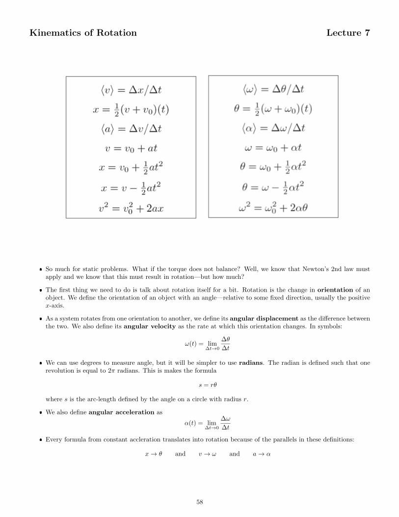
� So much for static problems. What if the torque does not balance? Well, we know that Newton’s 2nd law mustapply and we know that this must result in rotation—but how much?

� The first thing we need to do is talk about rotation itself for a bit. Rotation is the change in orientation of anobject. We define the orientation of an object with an angle—relative to some fixed direction, usually the positivex-axis.

� As a system rotates from one orientation to another, we define its angular displacement as the difference betweenthe two. We also define its angular velocity as the rate at which this orientation changes. In symbols:

ω(t) = lim∆t→0

∆θ

∆t

� We can use degrees to measure angle, but it will be simpler to use radians. The radian is defined such that onerevolution is equal to 2π radians. This is makes the formula

s = rθ

where s is the arc-length defined by the angle on a circle with radius r.

� We also define angular acceleration as

α(t) = lim∆t→0

∆ω

∆t

� Every formula from constant accleration translates into rotation because of the parallels in these definitions:

x→ θ and v → ω and a→ α

58

Moment of Inertia Lecture 7

� Consider, for a moment, a particle constrained to rotate around some pivot (maybe its connected by a thin metalrod, or something).

� If we apply a force to this particle, it will accelerate according to Newton’s 2nd law.

� But the constraint will counter-balance the component away from or toward the pivot. Only the component tangentto rotation will drive rotation.

� If we multiply both sides of Newton’s 2nd law with r (the distance to the pivot), we get

Ftr = mv2α

because a = rα.

� The left-hand-side is torque and the mr2 factor is called the moment of inertia for the particle. Similar to mass,this quantifies the rotational inertia of the particle around the pivot.

� A rigid objecgt can be seen as a collection of particles rotating in tandem. So, we can write

τ = Iα

where the moment of inertia is defined asI =

∑mr2

� It is occasionally useful to define the radius of gyration so that I = Mr2g where M is the total mass of the object.

This represents the radius of the ring with the same moment of inertia as the original object.

� We also define the angular momentum of an object as L = Iω.

59

Mechanical Analogies Lecture 7

� With the moment of inertia, we are ready to extend our analogy between linear and rotational motion:

F → τ and m→ I and p→ L

� Remember, the analogy works because of the parallel ways in which the quantities are defined. In particular, wecan also talk about the work associated with torque and rotation:

W = τ∆θ

� It follows that the kinetic energy of rotation is

KErot = 12Iω

2

� The “analogy” between rotation and linear motion is an example of an advanced technique of analysis calledgeneralized coordinates. The basic idea is that in a constrained system, the motion of the system is limited incertain ways defined by the constraint.

� Rather than expressing those constraints through forces, we represent them in the coordinates describing the motionand configuration of the system. These are called the degrees of freedom for the system.

– This is what we have done with the rigid body: rather than specify the intermolecular forces holding theobject together, we represent its motion through an angle.

– Essentially we define a momentum for these degrees of freedom and a form of Newton’s 2nd law still tells usthat generalized force changes this generalized momentum.

– These Euler-Lagrange equations naturally incorporate the inertial forces introduced though the non-inertialframe associated with the constrained coordinates.

60

Rolling Things Lecture 7

� One interesting problem in rotation is dealing with things that roll.

� This is the first time we are discussing an object that is both moving and rotating. As such, we will subscript thebulk motion with “cm” which stands for center of mass.

� Note that rolling is a condition that is between slipping and sliding.

– When an object slips, it is rotating too fast—like squealing tires.

– When an object slides, it is rotating too slow—like hydroplaning tires.

� The requirement is that the tangential velocity of the object be equal to the overall velocity of the object:

vcm = vt = rω

� It is of some interest to note that the rolling is accomplished by static friction. Kinetic friction is in play if theobject is slipping or sliding.

61

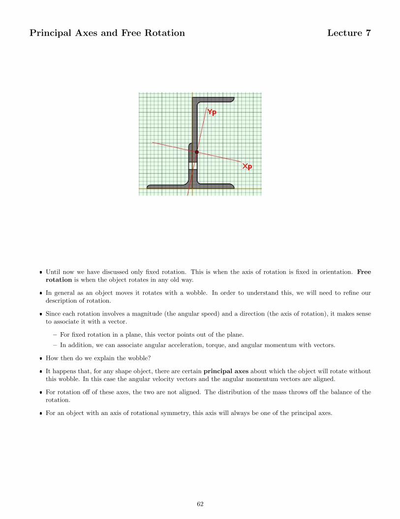
Principal Axes and Free Rotation Lecture 7

� Until now we have discussed only fixed rotation. This is when the axis of rotation is fixed in orientation. Freerotation is when the object rotates in any old way.

� In general as an object moves it rotates with a wobble. In order to understand this, we will need to refine ourdescription of rotation.

� Since each rotation involves a magnitude (the angular speed) and a direction (the axis of rotation), it makes senseto associate it with a vector.

– For fixed rotation in a plane, this vector points out of the plane.

– In addition, we can associate angular acceleration, torque, and angular momentum with vectors.

� How then do we explain the wobble?

� It happens that, for any shape object, there are certain principal axes about which the object will rotate withoutthis wobble. In this case the angular velocity vectors and the angular momentum vectors are aligned.

� For rotation off of these axes, the two are not aligned. The distribution of the mass throws off the balance of therotation.

� For an object with an axis of rotational symmetry, this axis will always be one of the principal axes.

62

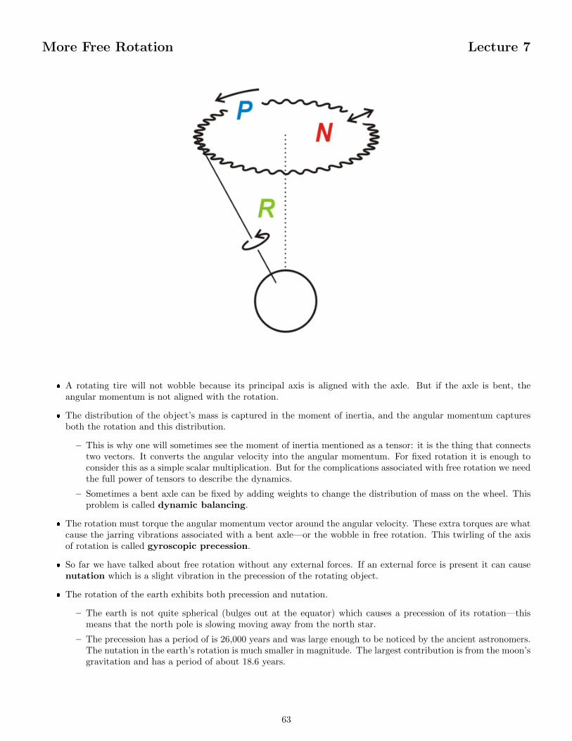
More Free Rotation Lecture 7

� A rotating tire will not wobble because its principal axis is aligned with the axle. But if the axle is bent, theangular momentum is not aligned with the rotation.

� The distribution of the object’s mass is captured in the moment of inertia, and the angular momentum capturesboth the rotation and this distribution.

– This is why one will sometimes see the moment of inertia mentioned as a tensor: it is the thing that connectstwo vectors. It converts the angular velocity into the angular momentum. For fixed rotation it is enough toconsider this as a simple scalar multiplication. But for the complications associated with free rotation we needthe full power of tensors to describe the dynamics.

– Sometimes a bent axle can be fixed by adding weights to change the distribution of mass on the wheel. Thisproblem is called dynamic balancing.

� The rotation must torque the angular momentum vector around the angular velocity. These extra torques are whatcause the jarring vibrations associated with a bent axle—or the wobble in free rotation. This twirling of the axisof rotation is called gyroscopic precession.

� So far we have talked about free rotation without any external forces. If an external force is present it can causenutation which is a slight vibration in the precession of the rotating object.

� The rotation of the earth exhibits both precession and nutation.

– The earth is not quite spherical (bulges out at the equator) which causes a precession of its rotation—thismeans that the north pole is slowing moving away from the north star.

– The precession has a period of is 26,000 years and was large enough to be noticed by the ancient astronomers.The nutation in the earth’s rotation is much smaller in magnitude. The largest contribution is from the moon’sgravitation and has a period of about 18.6 years.

63

Work, Power, and Energy Lecture 8

� Back to Earth...

� We return to a topic touched on previously: the mechanical advantage of simple machines. In this way we willmotivate the definitions of work, power, and energy.

� This will actually provide us a different way of analyzing the motion of particles. With advantages and disad-vantages, this energy framework adds some powerful tools to our “toolbox” for analyzing the motion of materialsystems.

64

Machines and Mechanical Advantage Lecture 8

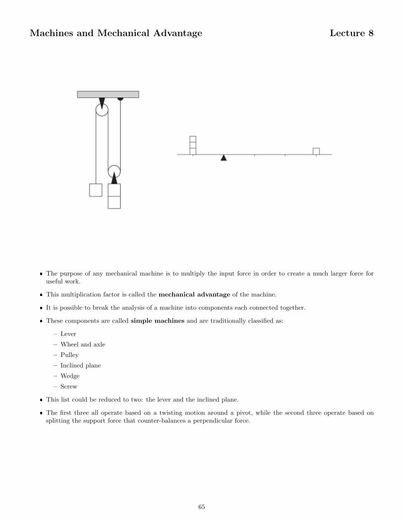
� The purpose of any mechanical machine is to multiply the input force in order to create a much larger force foruseful work.

� This multiplication factor is called the mechanical advantage of the machine.

� It is possible to break the analysis of a machine into components each connected together.

� These components are called simple machines and are traditionally classified as:

– Lever

– Wheel and axle

– Pulley

– Inclined plane

– Wedge

– Screw

� This list could be reduced to two: the lever and the inclined plane.

� The first three all operate based on a twisting motion around a pivot, while the second three operate based onsplitting the support force that counter-balances a perpendicular force.

65

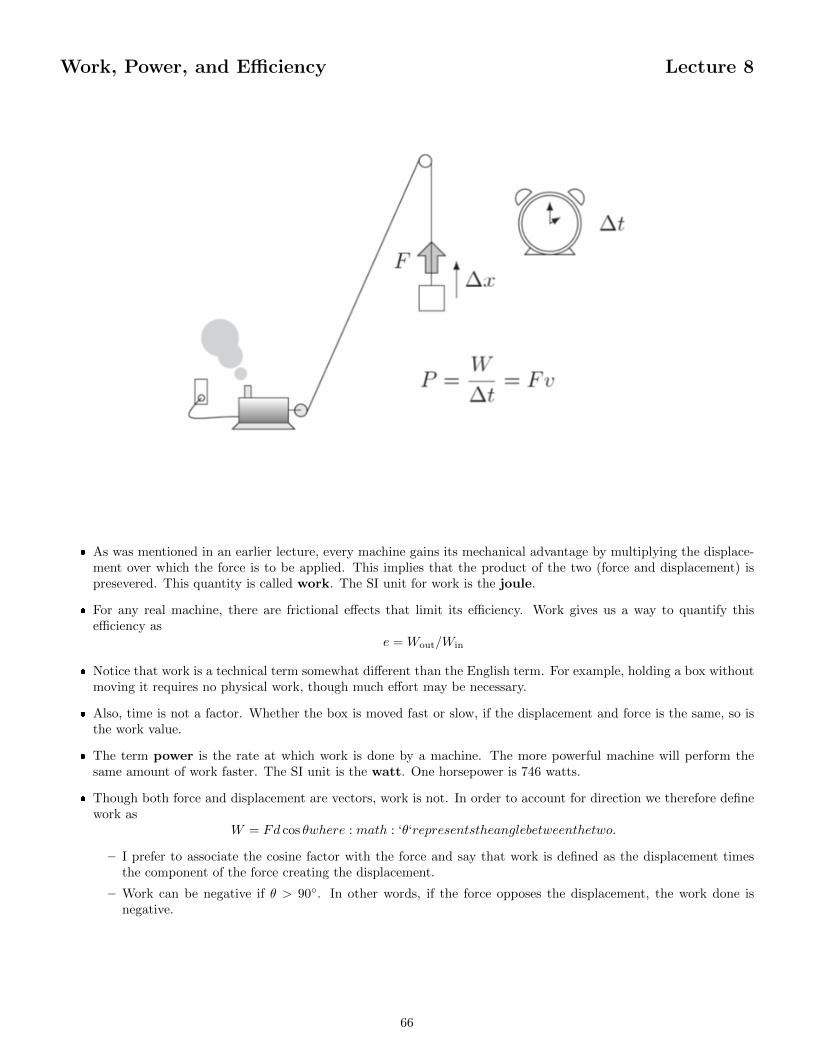
Work, Power, and Efficiency Lecture 8

� As was mentioned in an earlier lecture, every machine gains its mechanical advantage by multiplying the displace-ment over which the force is to be applied. This implies that the product of the two (force and displacement) ispresevered. This quantity is called work. The SI unit for work is the joule.

� For any real machine, there are frictional effects that limit its efficiency. Work gives us a way to quantify thisefficiency as

e = Wout/Win

� Notice that work is a technical term somewhat different than the English term. For example, holding a box withoutmoving it requires no physical work, though much effort may be necessary.

� Also, time is not a factor. Whether the box is moved fast or slow, if the displacement and force is the same, so isthe work value.

� The term power is the rate at which work is done by a machine. The more powerful machine will perform thesame amount of work faster. The SI unit is the watt. One horsepower is 746 watts.

� Though both force and displacement are vectors, work is not. In order to account for direction we therefore definework as

W = Fd cos θwhere : math : ‘θ‘representstheanglebetweenthetwo.

– I prefer to associate the cosine factor with the force and say that work is defined as the displacement timesthe component of the force creating the displacement.

– Work can be negative if θ > 90◦. In other words, if the force opposes the displacement, the work done isnegative.

66

Energy is the Ability to Do Work Lecture 8

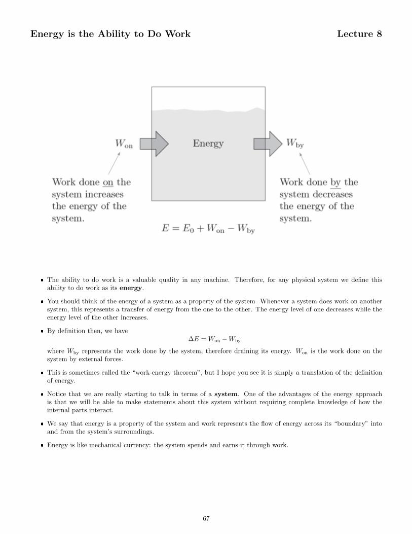
� The ability to do work is a valuable quality in any machine. Therefore, for any physical system we define thisability to do work as its energy.

� You should think of the energy of a system as a property of the system. Whenever a system does work on anothersystem, this represents a transfer of energy from the one to the other. The energy level of one decreases while theenergy level of the other increases.

� By definition then, we have∆E = Won −Wby

where Wby represents the work done by the system, therefore draining its energy. Won is the work done on thesystem by external forces.

� This is sometimes called the “work-energy theorem”, but I hope you see it is simply a translation of the definitionof energy.

� Notice that we are really starting to talk in terms of a system. One of the advantages of the energy approachis that we will be able to make statements about this system without requiring complete knowledge of how theinternal parts interact.

� We say that energy is a property of the system and work represents the flow of energy across its “boundary” intoand from the system’s surroundings.

� Energy is like mechanical currency: the system spends and earns it through work.

67

Kinetic Energy Defined Lecture 8

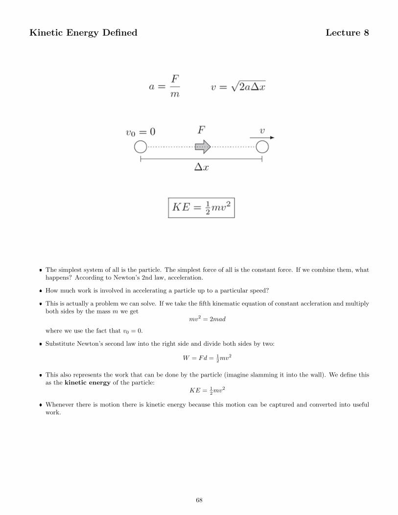
� The simplest system of all is the particle. The simplest force of all is the constant force. If we combine them, whathappens? According to Newton’s 2nd law, acceleration.

� How much work is involved in accelerating a particle up to a particular speed?

� This is actually a problem we can solve. If we take the fifth kinematic equation of constant accleration and multiplyboth sides by the mass m we get

mv2 = 2mad

where we use the fact that v0 = 0.

� Substitute Newton’s second law into the right side and divide both sides by two:

W = Fd = 12mv

2

� This also represents the work that can be done by the particle (imagine slamming it into the wall). We define thisas the kinetic energy of the particle:

KE = 12mv

2

� Whenever there is motion there is kinetic energy because this motion can be captured and converted into usefulwork.

68

Potential Energy Defined Lecture 8

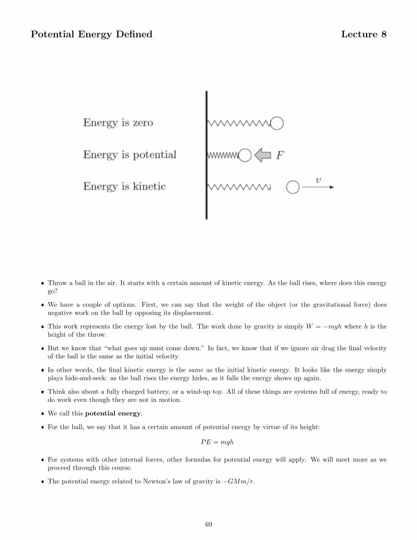
� Throw a ball in the air. It starts with a certain amount of kinetic energy. As the ball rises, where does this energygo?

� We have a couple of options. First, we can say that the weight of the object (or the gravitational force) doesnegative work on the ball by opposing its displacement.

� This work represents the energy lost by the ball. The work done by gravity is simply W = −mgh where h is theheight of the throw.

� But we know that “what goes up must come down.” In fact, we know that if we ignore air drag the final velocityof the ball is the same as the initial velocity.

� In other words, the final kinetic energy is the same as the initial kinetic energy. It looks like the energy simplyplays hide-and-seek: as the ball rises the energy hides, as it falls the energy shows up again.

� Think also about a fully charged battery, or a wind-up toy. All of these things are systems full of energy, ready todo work even though they are not in motion.

� We call this potential energy.

� For the ball, we say that it has a certain amount of potential energy by virtue of its height:

PE = mgh

� For systems with other internal forces, other formulas for potential energy will apply. We will meet more as weproceed through this course.

� The potential energy related to Newton’s law of gravity is −GMm/r.

69

Conservation of Energy Lecture 8

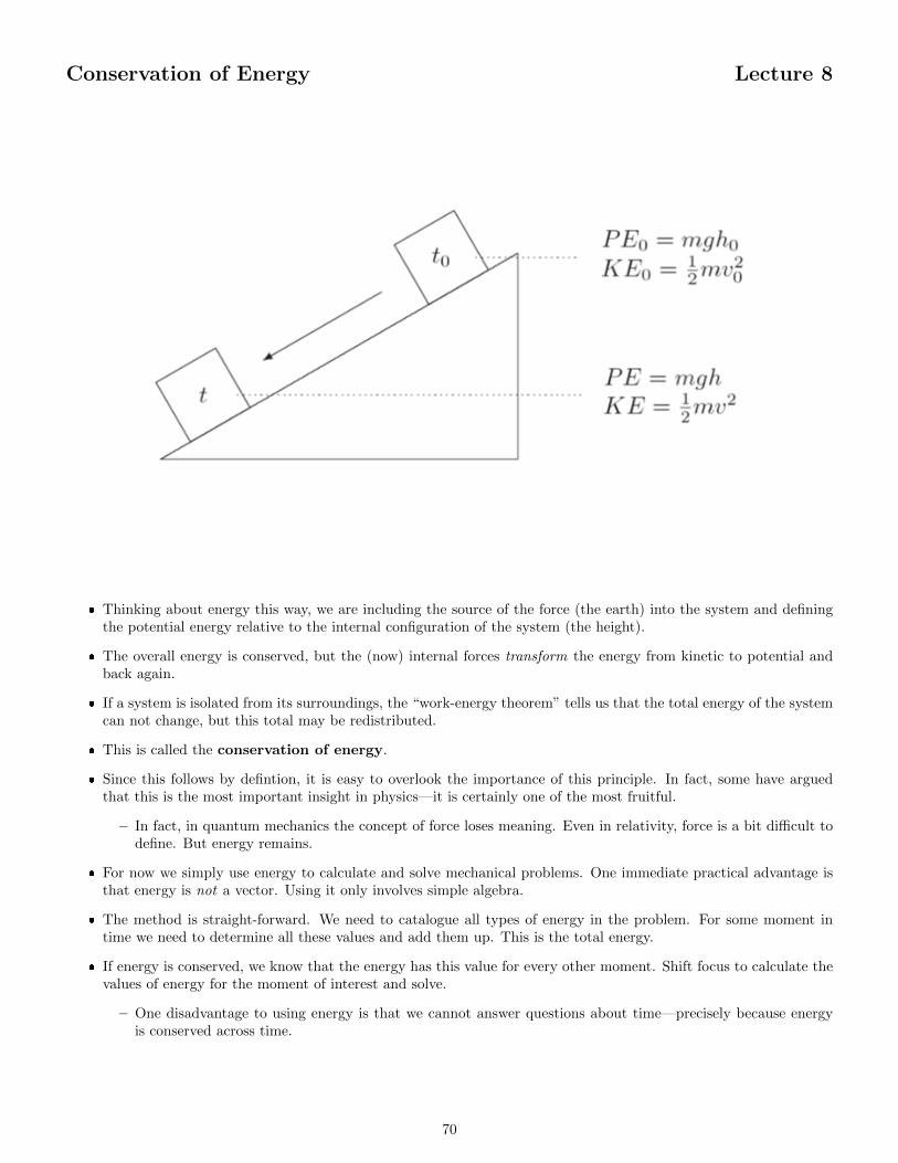
� Thinking about energy this way, we are including the source of the force (the earth) into the system and definingthe potential energy relative to the internal configuration of the system (the height).

� The overall energy is conserved, but the (now) internal forces transform the energy from kinetic to potential andback again.

� If a system is isolated from its surroundings, the “work-energy theorem” tells us that the total energy of the systemcan not change, but this total may be redistributed.

� This is called the conservation of energy.

� Since this follows by defintion, it is easy to overlook the importance of this principle. In fact, some have arguedthat this is the most important insight in physics—it is certainly one of the most fruitful.

– In fact, in quantum mechanics the concept of force loses meaning. Even in relativity, force is a bit difficult todefine. But energy remains.

� For now we simply use energy to calculate and solve mechanical problems. One immediate practical advantage isthat energy is not a vector. Using it only involves simple algebra.

� The method is straight-forward. We need to catalogue all types of energy in the problem. For some moment intime we need to determine all these values and add them up. This is the total energy.

� If energy is conserved, we know that the energy has this value for every other moment. Shift focus to calculate thevalues of energy for the moment of interest and solve.

– One disadvantage to using energy is that we cannot answer questions about time—precisely because energyis conserved across time.

70

Non-Conservative Forces Lecture 8

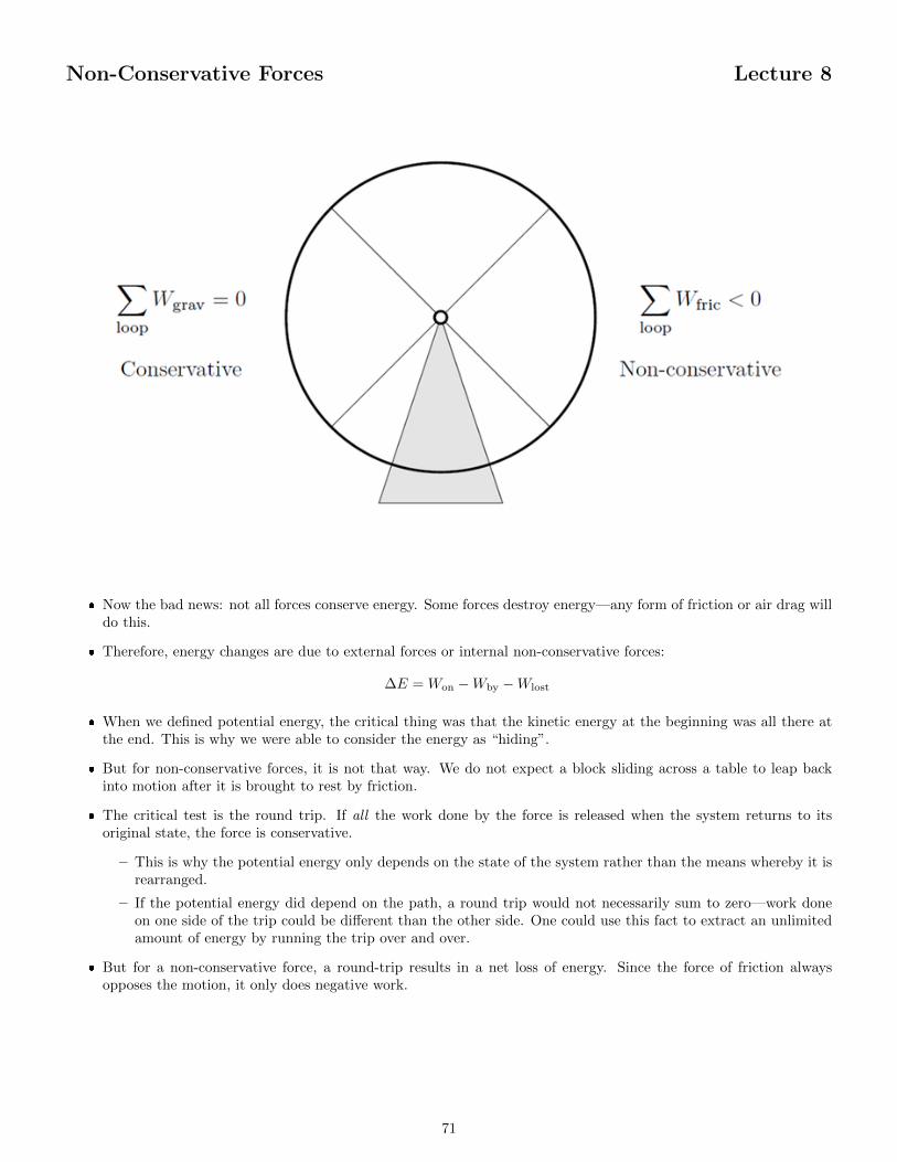
� Now the bad news: not all forces conserve energy. Some forces destroy energy—any form of friction or air drag willdo this.

� Therefore, energy changes are due to external forces or internal non-conservative forces:

∆E = Won −Wby −Wlost

� When we defined potential energy, the critical thing was that the kinetic energy at the beginning was all there atthe end. This is why we were able to consider the energy as “hiding”.

� But for non-conservative forces, it is not that way. We do not expect a block sliding across a table to leap backinto motion after it is brought to rest by friction.

� The critical test is the round trip. If all the work done by the force is released when the system returns to itsoriginal state, the force is conservative.

– This is why the potential energy only depends on the state of the system rather than the means whereby it isrearranged.

– If the potential energy did depend on the path, a round trip would not necessarily sum to zero—work doneon one side of the trip could be different than the other side. One could use this fact to extract an unlimitedamount of energy by running the trip over and over.

� But for a non-conservative force, a round-trip results in a net loss of energy. Since the force of friction alwaysopposes the motion, it only does negative work.

71

Energy Diagrams Lecture 8

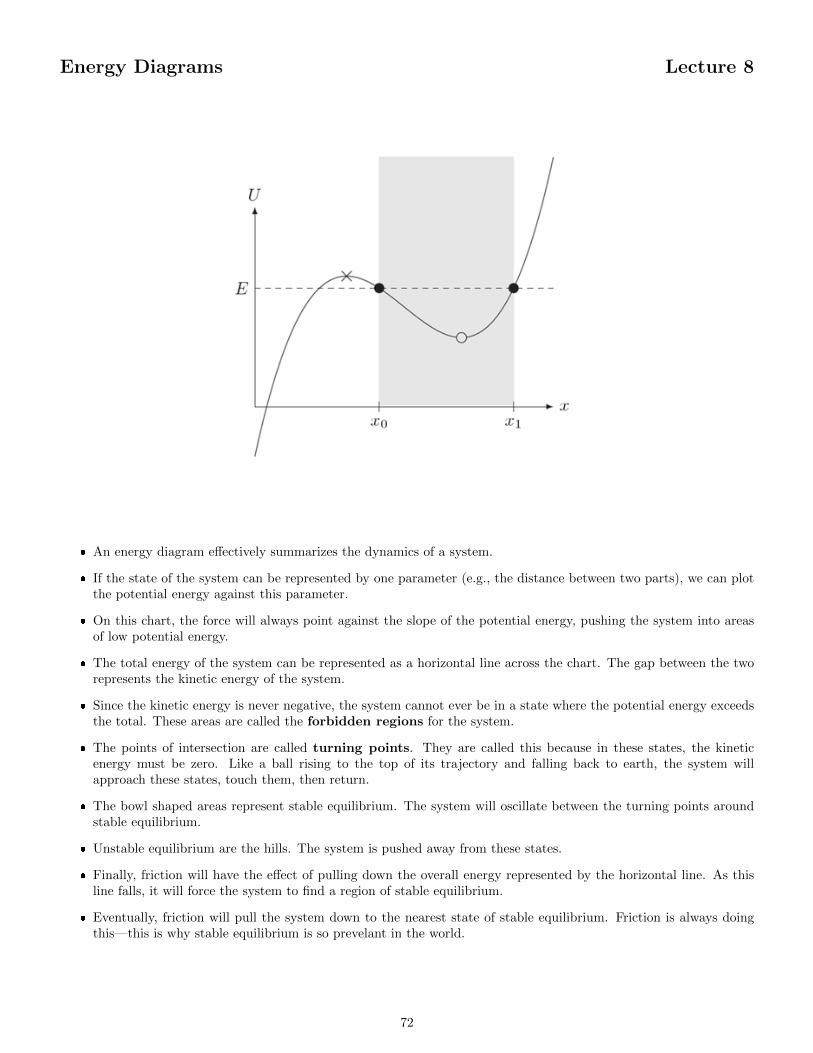
� An energy diagram effectively summarizes the dynamics of a system.

� If the state of the system can be represented by one parameter (e.g., the distance between two parts), we can plotthe potential energy against this parameter.

� On this chart, the force will always point against the slope of the potential energy, pushing the system into areasof low potential energy.

� The total energy of the system can be represented as a horizontal line across the chart. The gap between the tworepresents the kinetic energy of the system.

� Since the kinetic energy is never negative, the system cannot ever be in a state where the potential energy exceedsthe total. These areas are called the forbidden regions for the system.

� The points of intersection are called turning points. They are called this because in these states, the kineticenergy must be zero. Like a ball rising to the top of its trajectory and falling back to earth, the system willapproach these states, touch them, then return.

� The bowl shaped areas represent stable equilibrium. The system will oscillate between the turning points aroundstable equilibrium.

� Unstable equilibrium are the hills. The system is pushed away from these states.

� Finally, friction will have the effect of pulling down the overall energy represented by the horizontal line. As thisline falls, it will force the system to find a region of stable equilibrium.

� Eventually, friction will pull the system down to the nearest state of stable equilibrium. Friction is always doingthis—this is why stable equilibrium is so prevelant in the world.

72

Interacting Systems Lecture 9

� So far we have mostly been talking about a single particle. In this lecture we discuss how multiple particle caninteract.

� This is a more modern view: in quantum mechanics and relativity, the concept of force acting on a particle isreplaced with the idea of a system of particles interacting with one another.

� Especially in quantum field theory, where every fundamental force represents an interaction. And these interactionsare all mediated by exchange particles. Virtual particles flying back-and-forth exchanging properties between otherparticles.

� In this lecture we begin that story. And the beginning is in the definition of momentum.

73

Impulse Changes Momentum Lecture 9

� Momentum quantifies motion. It’s the combination of mass and velocity:

p = mv

� Notice that momentum is a vector quantity.

� In fact, Newton’s original formulation of his 2nd law was in terms of momentum. He wrote:

F =∆(mv)

∆t

� We can summarize this by simply saying that force is the rate at which momentum changes. The standard F = mafollows if the mass is considered constant.

� We can rewrite this formulation of Newton’s 2nd law in the following way:

F∆t = ∆(mv)

� The left-hand-side of this equation is called impulse and is useful to characterize quick bursts of force—like onesees in a collision. Newton’s 2nd law therefore states that impulse changes momentum.

– Impulse is usually given the symbol J , so we can rewrite this as J = ∆p.

– Actually, we don’t use impulse a lot, so I have found it’s simpler just to keep writing it out, like the formulaabove.

74

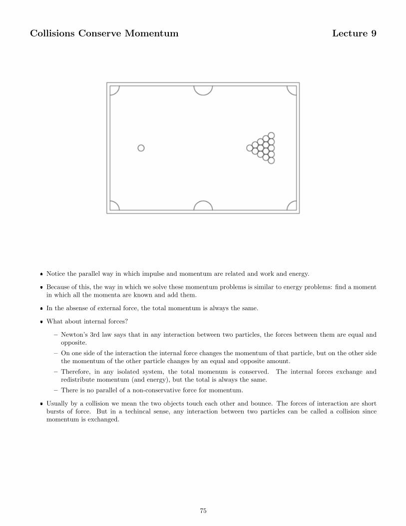
Collisions Conserve Momentum Lecture 9

� Notice the parallel way in which impulse and momentum are related and work and energy.

� Because of this, the way in which we solve these momentum problems is similar to energy problems: find a momentin which all the momenta are known and add them.

� In the absense of external force, the total momentum is always the same.

� What about internal forces?

– Newton’s 3rd law says that in any interaction between two particles, the forces between them are equal andopposite.

– On one side of the interaction the internal force changes the momentum of that particle, but on the other sidethe momentum of the other particle changes by an equal and opposite amount.

– Therefore, in any isolated system, the total momenum is conserved. The internal forces exchange andredistribute momentum (and energy), but the total is always the same.

– There is no parallel of a non-conservative force for momentum.

� Usually by a collision we mean the two objects touch each other and bounce. The forces of interaction are shortbursts of force. But in a techincal sense, any interaction between two particles can be called a collision sincemomentum is exchanged.

75

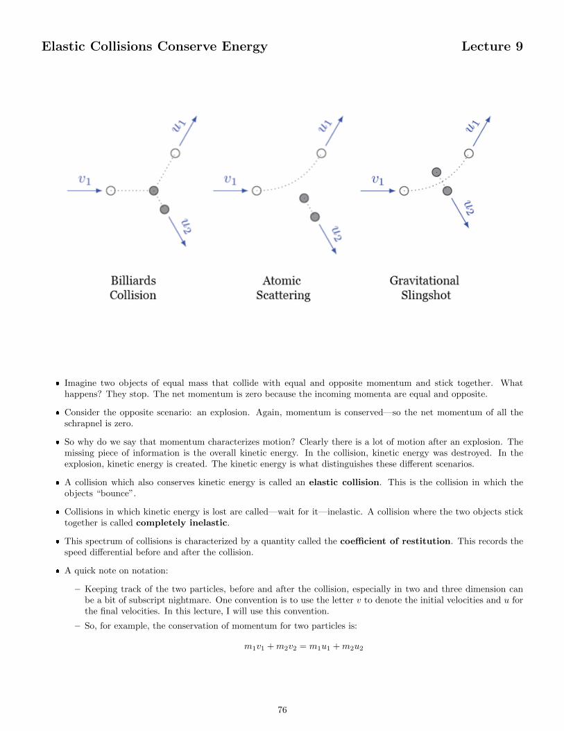
Elastic Collisions Conserve Energy Lecture 9

� Imagine two objects of equal mass that collide with equal and opposite momentum and stick together. Whathappens? They stop. The net momentum is zero because the incoming momenta are equal and opposite.

� Consider the opposite scenario: an explosion. Again, momentum is conserved—so the net momentum of all theschrapnel is zero.

� So why do we say that momentum characterizes motion? Clearly there is a lot of motion after an explosion. Themissing piece of information is the overall kinetic energy. In the collision, kinetic energy was destroyed. In theexplosion, kinetic energy is created. The kinetic energy is what distinguishes these different scenarios.

� A collision which also conserves kinetic energy is called an elastic collision. This is the collision in which theobjects “bounce”.

� Collisions in which kinetic energy is lost are called—wait for it—inelastic. A collision where the two objects sticktogether is called completely inelastic.

� This spectrum of collisions is characterized by a quantity called the coefficient of restitution. This records thespeed differential before and after the collision.

� A quick note on notation:

– Keeping track of the two particles, before and after the collision, especially in two and three dimension canbe a bit of subscript nightmare. One convention is to use the letter v to denote the initial velocities and u forthe final velocities. In this lecture, I will use this convention.

– So, for example, the conservation of momentum for two particles is:

m1v1 +m2v2 = m1u1 +m2u2

76

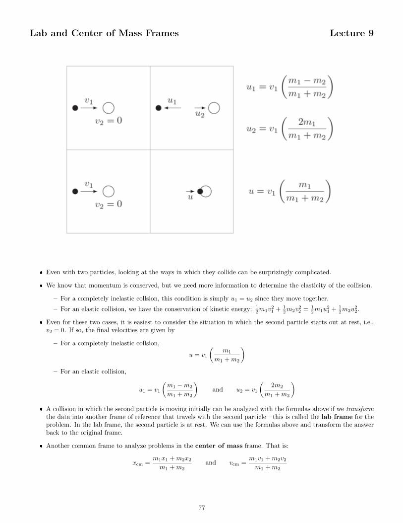
Lab and Center of Mass Frames Lecture 9

� Even with two particles, looking at the ways in which they collide can be surprizingly complicated.

� We know that momentum is conserved, but we need more information to determine the elasticity of the collision.

– For a completely inelastic collsion, this condition is simply u1 = u2 since they move together.

– For an elastic collision, we have the conservation of kinetic energy: 12m1v

21 + 1

2m2v22 = 1

2m1u21 + 1

2m2u22.

� Even for these two cases, it is easiest to consider the situation in which the second particle starts out at rest, i.e.,v2 = 0. If so, the final velocities are given by

– For a completely inelastic collsion,

u = v1

(m1

m1 +m2

)– For an elastic collision,

u1 = v1

(m1 −m2

m1 +m2

)and u2 = v1

(2m2

m1 +m2

)� A collision in which the second particle is moving initially can be analyzed with the formulas above if we transform

the data into another frame of reference that travels with the second particle—this is called the lab frame for theproblem. In the lab frame, the second particle is at rest. We can use the formulas above and transform the answerback to the original frame.

� Another common frame to analyze problems in the center of mass frame. That is:

xcm =m1x1 +m2x2

m1 +m2and vcm =

m1v1 +m2v2

m1 +m2

77

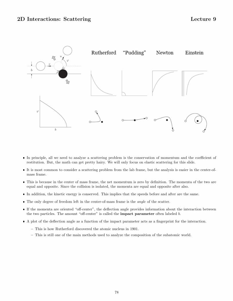
2D Interactions: Scattering Lecture 9

� In principle, all we need to analyze a scattering problem is the conservation of momentum and the coefficient ofrestitution. But, the math can get pretty hairy. We will only focus on elastic scattering for this slide.

� It is most common to consider a scattering problem from the lab frame, but the analysis is easier in the center-of-mass frame.

� This is because in the center of mass frame, the net momentum is zero by definition. The momenta of the two areequal and opposite. Since the collision is isolated, the momenta are equal and opposite after also.

� In addition, the kinetic energy is conserved. This implies that the speeds before and after are the same.

� The only degree of freedom left in the center-of-mass frame is the angle of the scatter.

� If the momenta are oriented “off-center”, the deflection angle provides information about the interaction betweenthe two particles. The amount “off-center” is called the impact parameter often labeled b.

� A plot of the deflection angle as a function of the impact parameter acts as a fingerprint for the interaction.

– This is how Rutherford discovered the atomic nucleus in 1901.

– This is still one of the main methods used to analyze the composition of the subatomic world.

78

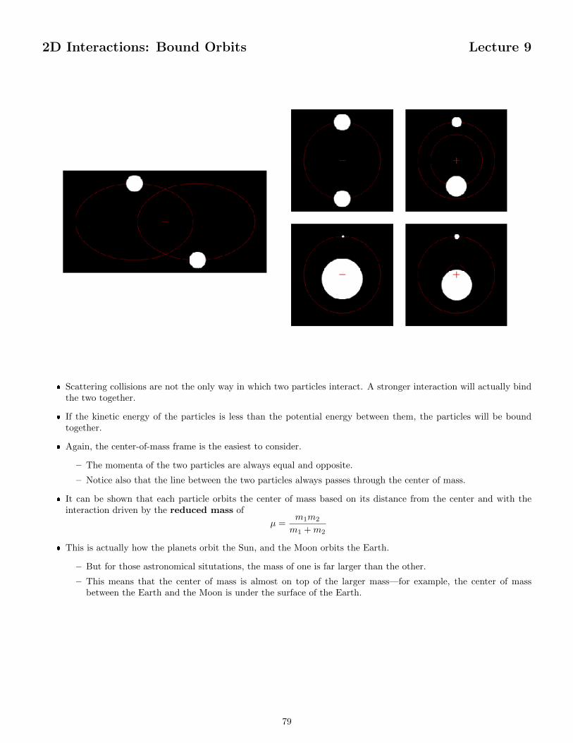
2D Interactions: Bound Orbits Lecture 9

� Scattering collisions are not the only way in which two particles interact. A stronger interaction will actually bindthe two together.

� If the kinetic energy of the particles is less than the potential energy between them, the particles will be boundtogether.

� Again, the center-of-mass frame is the easiest to consider.

– The momenta of the two particles are always equal and opposite.

– Notice also that the line between the two particles always passes through the center of mass.

� It can be shown that each particle orbits the center of mass based on its distance from the center and with theinteraction driven by the reduced mass of

µ =m1m2

m1 +m2

� This is actually how the planets orbit the Sun, and the Moon orbits the Earth.

– But for those astronomical situtations, the mass of one is far larger than the other.

– This means that the center of mass is almost on top of the larger mass—for example, the center of massbetween the Earth and the Moon is under the surface of the Earth.

79

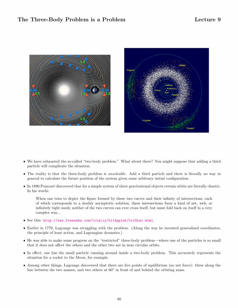
The Three-Body Problem is a Problem Lecture 9

� We have exhausted the so-called “two-body problem.” What about three? You might suppose that adding a thirdparticle will complicate the situation.

� The reality is that the three-body problem is unsolvable. Add a third particle and there is literally no way ingeneral to calculate the future position of the system given some arbitrary initial configuration.

� In 1890 Poincare discovered that for a simple system of three gravitational objects certain orbits are literally chaotic.In his words:

When one tries to depict the figure formed by these two curves and their infinity of intersections, eachof which corresponds to a doubly asymptotic solution, these intersections form a kind of net, web, orinfinitely tight mesh; neither of the two curves can ever cross itself, but must fold back on itself in a verycomplex way...

� See this: http://www.freewebz.com/vitaliy/triApplet/triGrav.html.

� Earlier in 1770, Lagrange was struggling with the problem. (Along the way he invented generalized coordinates,the principle of least action, and Lagrangian dynamics.)

� He was able to make some progress on the “restricted” three-body problem—where one of the particles is so smallthat it does not affect the others and the other two are in near circular orbits.

� In effect, one has the small particle running around inside a two-body problem. This accurately represents thesituation for a rocket to the Moon, for example.

� Among other things, Lagrange discovered that there are five points of equilibrium (no net force): three along theline between the two masses, and two others at 60◦ in front of and behind the orbiting mass.

80

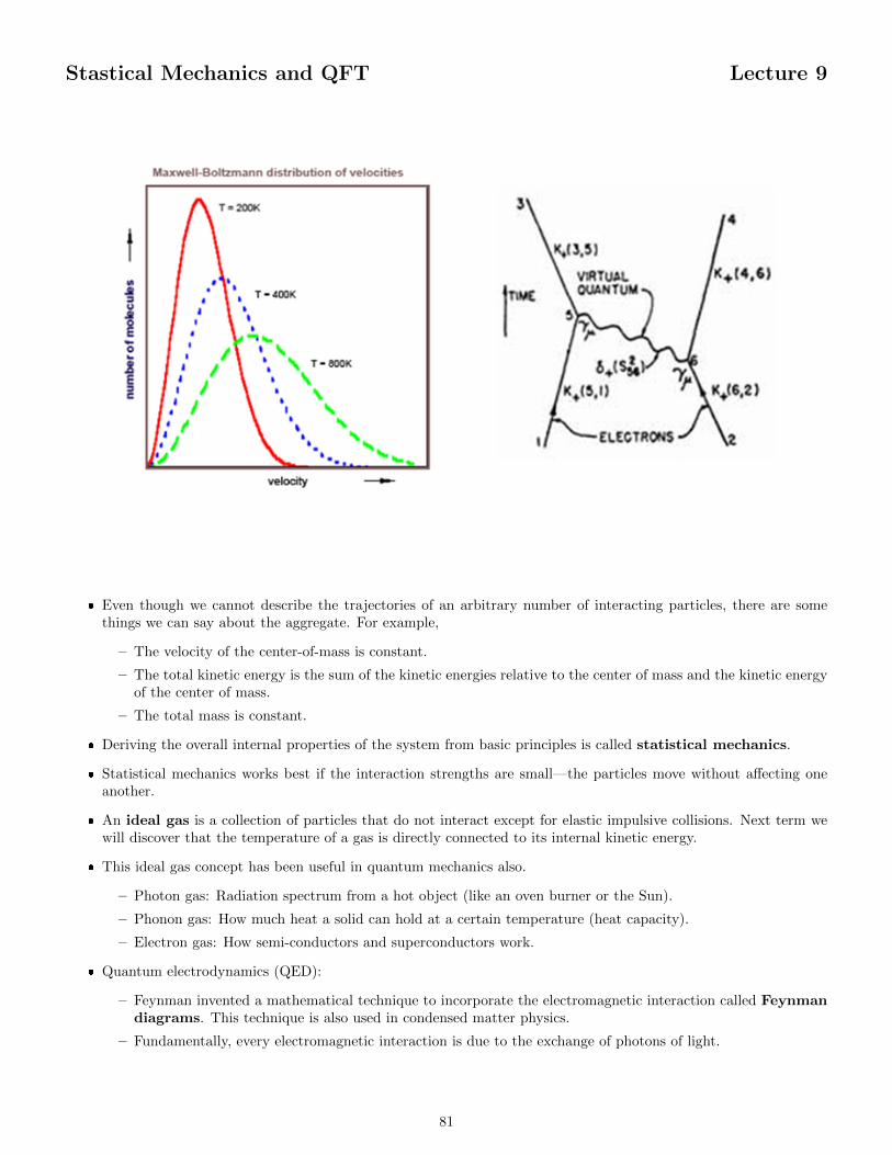
Stastical Mechanics and QFT Lecture 9

� Even though we cannot describe the trajectories of an arbitrary number of interacting particles, there are somethings we can say about the aggregate. For example,

– The velocity of the center-of-mass is constant.

– The total kinetic energy is the sum of the kinetic energies relative to the center of mass and the kinetic energyof the center of mass.

– The total mass is constant.

� Deriving the overall internal properties of the system from basic principles is called statistical mechanics.

� Statistical mechanics works best if the interaction strengths are small—the particles move without affecting oneanother.

� An ideal gas is a collection of particles that do not interact except for elastic impulsive collisions. Next term wewill discover that the temperature of a gas is directly connected to its internal kinetic energy.

� This ideal gas concept has been useful in quantum mechanics also.

– Photon gas: Radiation spectrum from a hot object (like an oven burner or the Sun).

– Phonon gas: How much heat a solid can hold at a certain temperature (heat capacity).

– Electron gas: How semi-conductors and superconductors work.

� Quantum electrodynamics (QED):

– Feynman invented a mathematical technique to incorporate the electromagnetic interaction called Feynmandiagrams. This technique is also used in condensed matter physics.

– Fundamentally, every electromagnetic interaction is due to the exchange of photons of light.

81

Celestial Mechanics Lecture 10

� This is the first of two topics which I have added to the curriculum for this term.

� We have a surprizing amount of firepower at our disposal to analyze some basic problems in celestial and orbitalmechanics.

� This lecture really is rocket science!

82

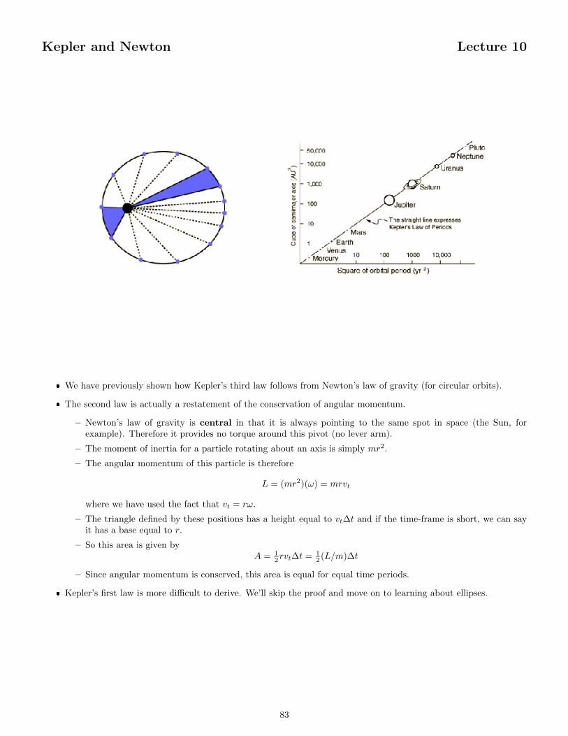
Kepler and Newton Lecture 10

� We have previously shown how Kepler’s third law follows from Newton’s law of gravity (for circular orbits).

� The second law is actually a restatement of the conservation of angular momentum.

– Newton’s law of gravity is central in that it is always pointing to the same spot in space (the Sun, forexample). Therefore it provides no torque around this pivot (no lever arm).

– The moment of inertia for a particle rotating about an axis is simply mr2.

– The angular momentum of this particle is therefore

L = (mr2)(ω) = mrvt

where we have used the fact that vt = rω.

– The triangle defined by these positions has a height equal to vt∆t and if the time-frame is short, we can sayit has a base equal to r.

– So this area is given byA = 1

2rvt∆t = 12 (L/m)∆t

– Since angular momentum is conserved, this area is equal for equal time periods.

� Kepler’s first law is more difficult to derive. We’ll skip the proof and move on to learning about ellipses.

83

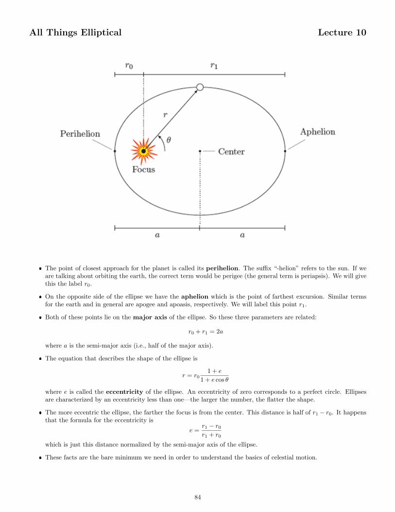
All Things Elliptical Lecture 10

� The point of closest approach for the planet is called its perihelion. The suffix “-helion” refers to the sun. If weare talking about orbiting the earth, the correct term would be perigee (the general term is periapsis). We will givethis the label r0.

� On the opposite side of the ellipse we have the aphelion which is the point of farthest excursion. Similar termsfor the earth and in general are apogee and apoasis, respectively. We will label this point r1.

� Both of these points lie on the major axis of the ellipse. So these three parameters are related:

r0 + r1 = 2a

where a is the semi-major axis (i.e., half of the major axis).

� The equation that describes the shape of the ellipse is

r = r01 + e

1 + e cos θ

where e is called the eccentricity of the ellipse. An eccentricity of zero corresponds to a perfect circle. Ellipsesare characterized by an eccentricity less than one—the larger the number, the flatter the shape.

� The more eccentric the ellipse, the farther the focus is from the center. This distance is half of r1 − r0. It happensthat the formula for the eccentricity is

e =r1 − r0

r1 + r0

which is just this distance normalized by the semi-major axis of the ellipse.

� These facts are the bare minimum we need in order to understand the basics of celestial motion.

84

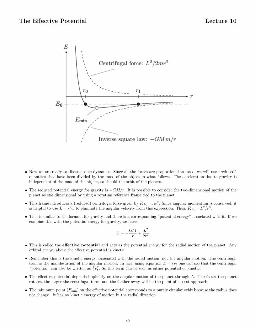
The Effective Potential Lecture 10

� Now we are ready to discuss some dynamics. Since all the forces are proportional to mass, we will use “reduced”quantites that have been divided by the mass of the object in what follows. The acceleration due to gravity isindependent of the mass of the object, so should the orbit of the planets.

� The reduced potential energy for gravity is −GM/r. It is possible to consider the two-dimensional motion of theplanet as one dimensional by using a rotating reference frame tied to the planet.

� This frame introduces a (reduced) centrifugal force given by Fcfg = rω2. Since angular momentum is conserved, itis helpful to use L = r2ω to eliminate the angular velocity from this expression. Thus, Fcfg = L2/r3.

� This is similar to the formula for gravity and there is a corresponding “potential energy” associated with it. If wecombine this with the potential energy for gravity, we have:

U = −GMr

+L2

2r2

� This is called the effective potential and acts as the potential energy for the radial motion of the planet. Anyorbital energy above the effective potential is kinetic.

� Remember this is the kinetic energy associated with the radial motion, not the angular motion. The centrifugalterm is the manifestation of the angular motion. In fact, using equation L = rvt one can see that the centrifugal“potential” can also be written as 1

2v2t . So this term can be seen as either potential or kinetic.

� The effective potential depends implicitly on the angular motion of the planet through L. The faster the planetrotates, the larger the centrifugal term, and the farther away will be the point of closest approach.

� The minimum point (Emin) on the effective potential corresponds to a purely circular orbit because the radius doesnot change—it has no kinetic energy of motion in the radial direction.

85

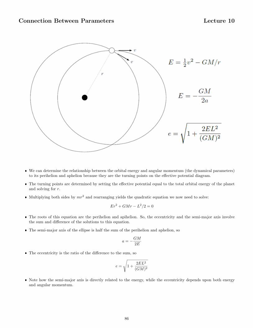
Connection Between Parameters Lecture 10

� We can determine the relationship between the orbital energy and angular momentum (the dynamical parameters)to its perihelion and aphelion because they are the turning points on the effective potential diagram.

� The turning points are determined by setting the effective potential equal to the total orbital energy of the planetand solving for r.

� Multiplying both sides by mr2 and rearranging yields the quadratic equation we now need to solve:

Er2 +GMr − L2/2 = 0

� The roots of this equation are the perihelion and apihelion. So, the eccentricity and the semi-major axis involvethe sum and difference of the solutions to this equation.

� The semi-major axis of the ellipse is half the sum of the perihelion and aphelion, so

a = −GM2E

� The eccentricity is the ratio of the difference to the sum, so

e =

√1 +

2EL2

(GM)2

� Note how the semi-major axis is directly related to the energy, while the eccentricity depends upon both energyand angular momentum.

86

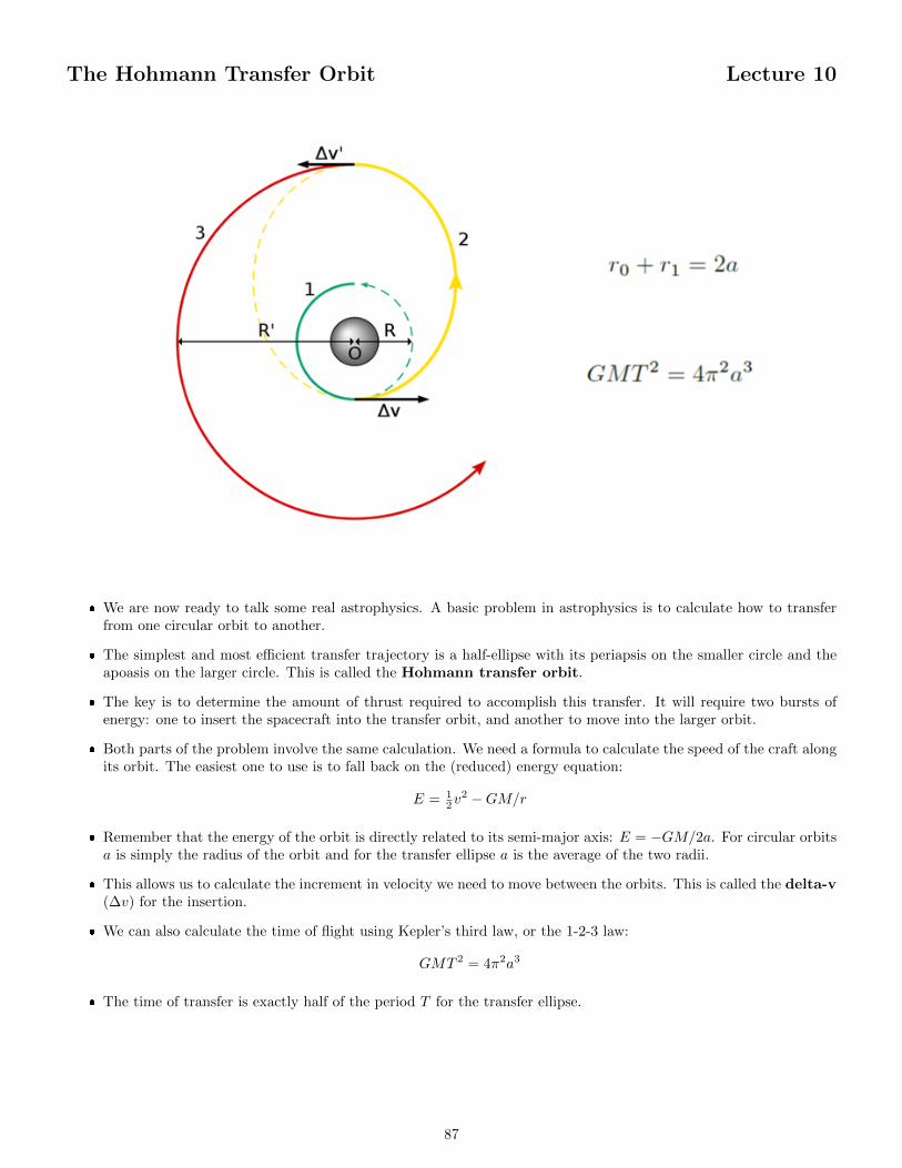
The Hohmann Transfer Orbit Lecture 10

� We are now ready to talk some real astrophysics. A basic problem in astrophysics is to calculate how to transferfrom one circular orbit to another.

� The simplest and most efficient transfer trajectory is a half-ellipse with its periapsis on the smaller circle and theapoasis on the larger circle. This is called the Hohmann transfer orbit.

� The key is to determine the amount of thrust required to accomplish this transfer. It will require two bursts ofenergy: one to insert the spacecraft into the transfer orbit, and another to move into the larger orbit.

� Both parts of the problem involve the same calculation. We need a formula to calculate the speed of the craft alongits orbit. The easiest one to use is to fall back on the (reduced) energy equation:

E = 12v

2 −GM/r

� Remember that the energy of the orbit is directly related to its semi-major axis: E = −GM/2a. For circular orbitsa is simply the radius of the orbit and for the transfer ellipse a is the average of the two radii.

� This allows us to calculate the increment in velocity we need to move between the orbits. This is called the delta-v(∆v) for the insertion.

� We can also calculate the time of flight using Kepler’s third law, or the 1-2-3 law:

GMT 2 = 4π2a3

� The time of transfer is exactly half of the period T for the transfer ellipse.

87

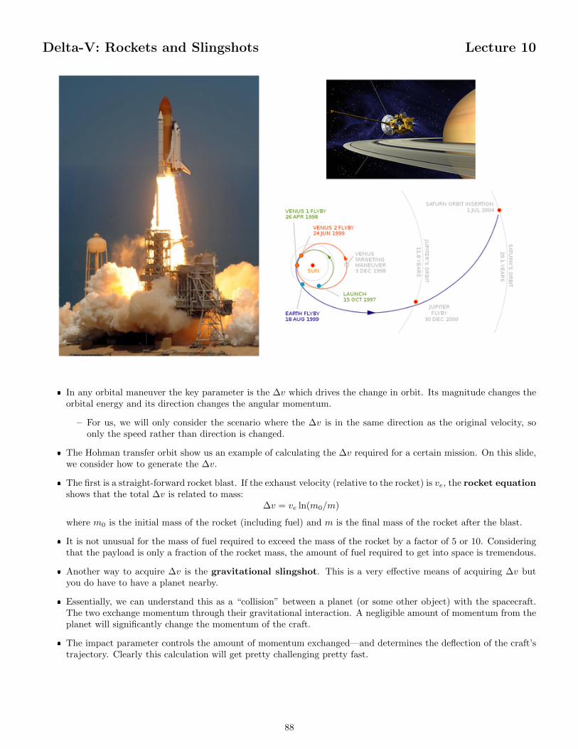
Delta-V: Rockets and Slingshots Lecture 10

� In any orbital maneuver the key parameter is the ∆v which drives the change in orbit. Its magnitude changes theorbital energy and its direction changes the angular momentum.

– For us, we will only consider the scenario where the ∆v is in the same direction as the original velocity, soonly the speed rather than direction is changed.

� The Hohman transfer orbit show us an example of calculating the ∆v required for a certain mission. On this slide,we consider how to generate the ∆v.

� The first is a straight-forward rocket blast. If the exhaust velocity (relative to the rocket) is ve, the rocket equationshows that the total ∆v is related to mass:

∆v = ve ln(m0/m)

where m0 is the initial mass of the rocket (including fuel) and m is the final mass of the rocket after the blast.

� It is not unusual for the mass of fuel required to exceed the mass of the rocket by a factor of 5 or 10. Consideringthat the payload is only a fraction of the rocket mass, the amount of fuel required to get into space is tremendous.

� Another way to acquire ∆v is the gravitational slingshot. This is a very effective means of acquiring ∆v butyou do have to have a planet nearby.

� Essentially, we can understand this as a “collision” between a planet (or some other object) with the spacecraft.The two exchange momentum through their gravitational interaction. A negligible amount of momentum from theplanet will significantly change the momentum of the craft.

� The impact parameter controls the amount of momentum exchanged—and determines the deflection of the craft’strajectory. Clearly this calculation will get pretty challenging pretty fast.

88

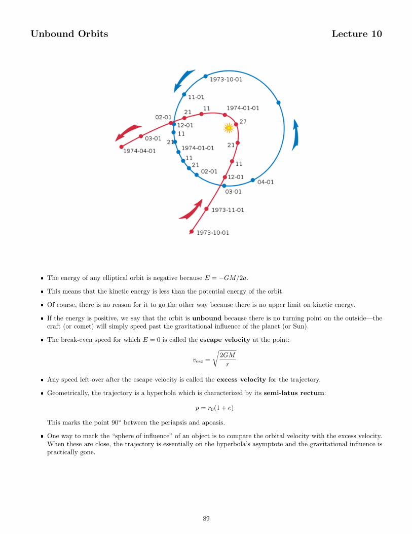
Unbound Orbits Lecture 10

� The energy of any elliptical orbit is negative because E = −GM/2a.

� This means that the kinetic energy is less than the potential energy of the orbit.

� Of course, there is no reason for it to go the other way because there is no upper limit on kinetic energy.

� If the energy is positive, we say that the orbit is unbound because there is no turning point on the outside—thecraft (or comet) will simply speed past the gravitational influence of the planet (or Sun).

� The break-even speed for which E = 0 is called the escape velocity at the point:

vesc =

√2GM

r

� Any speed left-over after the escape velocity is called the excess velocity for the trajectory.

� Geometrically, the trajectory is a hyperbola which is characterized by its semi-latus rectum:

p = r0(1 + e)

This marks the point 90◦ between the periapsis and apoasis.

� One way to mark the “sphere of influence” of an object is to compare the orbital velocity with the excess velocity.When these are close, the trajectory is essentially on the hyperbola’s asymptote and the gravitational influence ispractically gone.

89

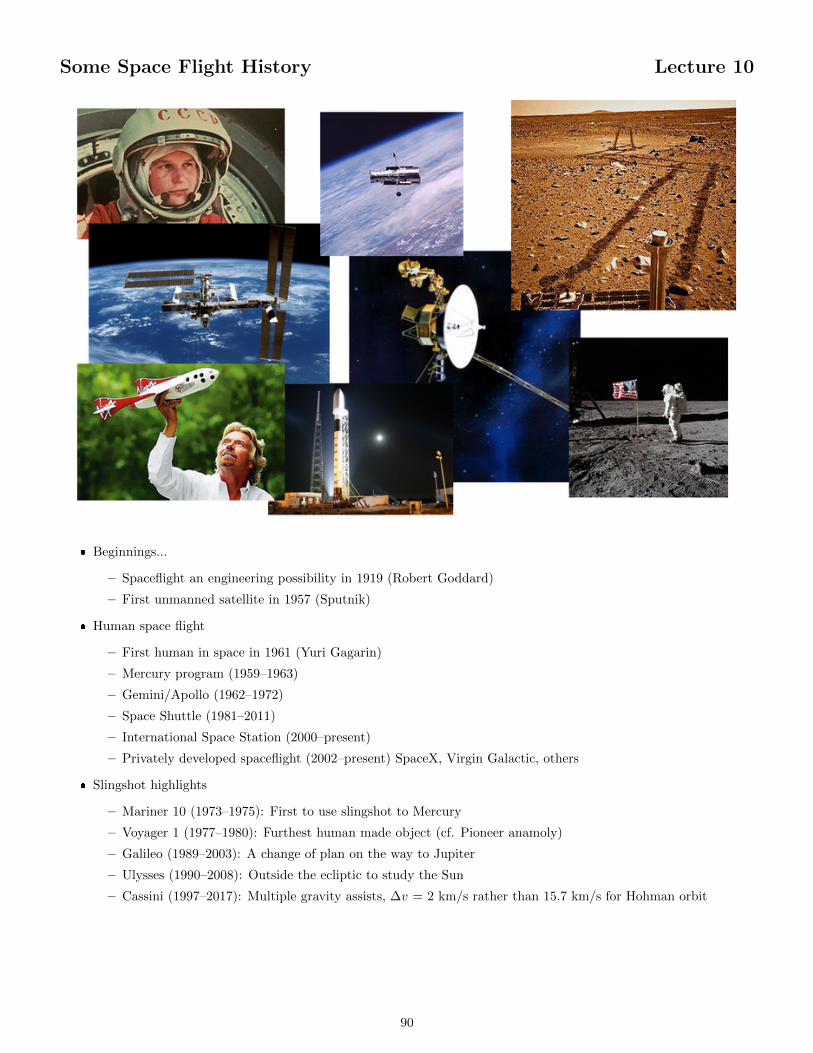
Some Space Flight History Lecture 10

� Beginnings...

– Spaceflight an engineering possibility in 1919 (Robert Goddard)

– First unmanned satellite in 1957 (Sputnik)

� Human space flight

– First human in space in 1961 (Yuri Gagarin)

– Mercury program (1959–1963)

– Gemini/Apollo (1962–1972)

– Space Shuttle (1981–2011)

– International Space Station (2000–present)

– Privately developed spaceflight (2002–present) SpaceX, Virgin Galactic, others

� Slingshot highlights

– Mariner 10 (1973–1975): First to use slingshot to Mercury

– Voyager 1 (1977–1980): Furthest human made object (cf. Pioneer anamoly)

– Galileo (1989–2003): A change of plan on the way to Jupiter

– Ulysses (1990–2008): Outside the ecliptic to study the Sun

– Cassini (1997–2017): Multiple gravity assists, ∆v = 2 km/s rather than 15.7 km/s for Hohman orbit

90

Bending Time Lecture 11

� In this final lecture of the term, we complete our study of celestial mechanics and gravity with a overview of generalrelativity.

� General relativity is notorious for being mathematically difficult. Obviously we will only be touching the highlightsand some results without deriving them.

� Also, we have not studied relativity!

� I’ve suspected for a while that there is a way to introduce the concepts of general relativity without the relativity.I think this lecture is the closest I’ve ever come to that goal.

� With that said, let’s dive in...

91

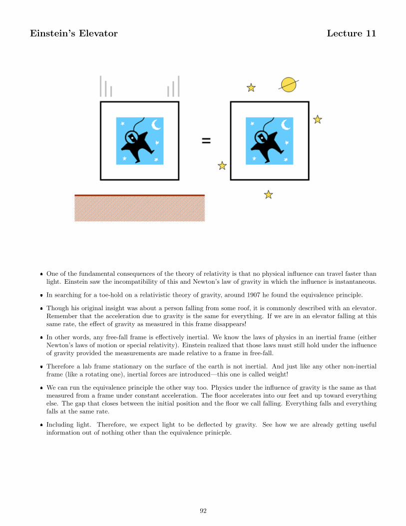
Einstein’s Elevator Lecture 11

� One of the fundamental consequences of the theory of relativity is that no physical influence can travel faster thanlight. Einstein saw the incompatibility of this and Newton’s law of gravity in which the influence is instantaneous.

� In searching for a toe-hold on a relativistic theory of gravity, around 1907 he found the equivalence principle.

� Though his original insight was about a person falling from some roof, it is commonly described with an elevator.Remember that the acceleration due to gravity is the same for everything. If we are in an elevator falling at thissame rate, the effect of gravity as measured in this frame disappears!

� In other words, any free-fall frame is effectively inertial. We know the laws of physics in an inertial frame (eitherNewton’s laws of motion or special relativity). Einstein realized that those laws must still hold under the influenceof gravity provided the measurements are made relative to a frame in free-fall.

� Therefore a lab frame stationary on the surface of the earth is not inertial. And just like any other non-inertialframe (like a rotating one), inertial forces are introduced—this one is called weight!

� We can run the equivalence principle the other way too. Physics under the influence of gravity is the same as thatmeasured from a frame under constant acceleration. The floor accelerates into our feet and up toward everythingelse. The gap that closes between the initial position and the floor we call falling. Everything falls and everythingfalls at the same rate.

� Including light. Therefore, we expect light to be deflected by gravity. See how we are already getting usefulinformation out of nothing other than the equivalence prinicple.

92

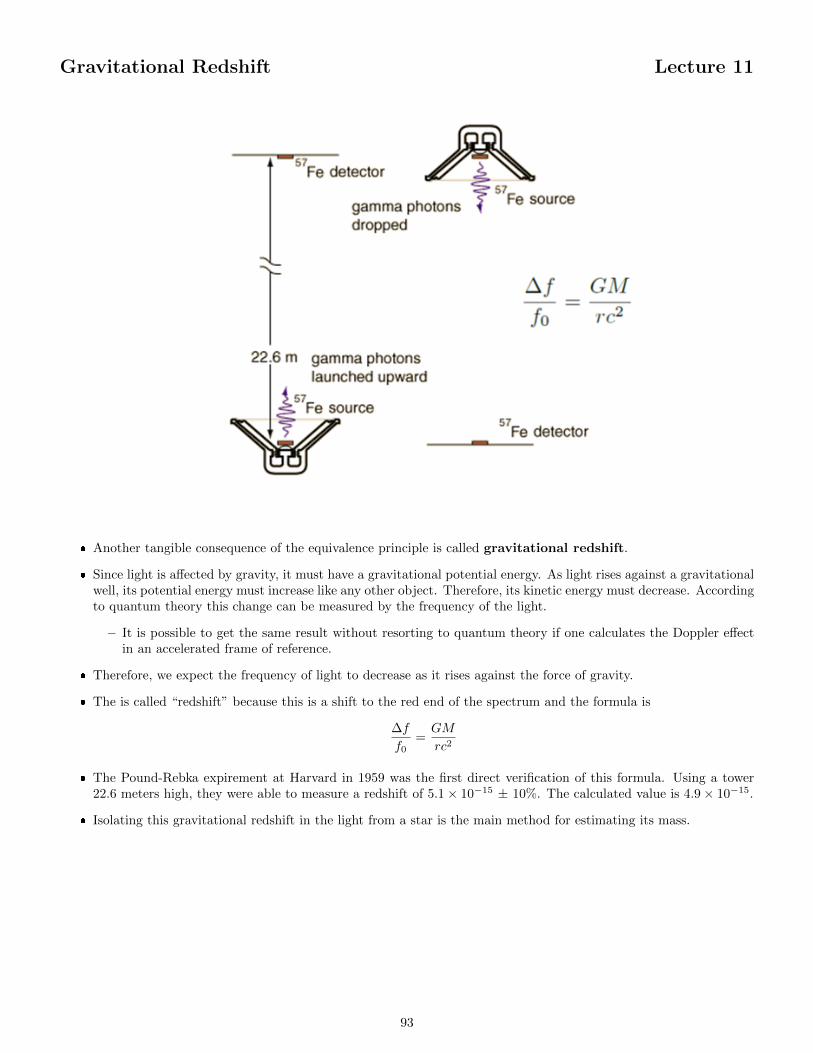
Gravitational Redshift Lecture 11

� Another tangible consequence of the equivalence principle is called gravitational redshift.

� Since light is affected by gravity, it must have a gravitational potential energy. As light rises against a gravitationalwell, its potential energy must increase like any other object. Therefore, its kinetic energy must decrease. Accordingto quantum theory this change can be measured by the frequency of the light.

– It is possible to get the same result without resorting to quantum theory if one calculates the Doppler effectin an accelerated frame of reference.

� Therefore, we expect the frequency of light to decrease as it rises against the force of gravity.

� The is called “redshift” because this is a shift to the red end of the spectrum and the formula is

∆f

f0=GM

rc2

� The Pound-Rebka expirement at Harvard in 1959 was the first direct verification of this formula. Using a tower22.6 meters high, they were able to measure a redshift of 5.1× 10−15 ± 10%. The calculated value is 4.9× 10−15.

� Isolating this gravitational redshift in the light from a star is the main method for estimating its mass.

93

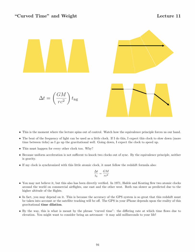
“Curved Time” and Weight Lecture 11

� This is the moment where the lecture spins out of control. Watch how the equivalence principle forces us our hand.

� The beat of the frequency of light can be used as a little clock. If I do this, I expect this clock to slow down (moretime between ticks) as I go up the gravitational well. Going down, I expect the clock to speed up.

� This must happen for every other clock too. Why?

� Because uniform acceleration is not sufficent to knock two clocks out of sync. By the equivalence principle, neitheris gravity.

� If my clock is synchronized with this little atomic clock, it must follow the redshift formula also:

∆t

t0=GM

rc2

� You may not believe it, but this also has been directly verified. In 1971, Hafele and Keating flew two atomic clocksaround the world on commercial airflights, one east and the other west. Both ran slower as predicted due to thehigher altitude of the flights.

� In fact, you may depend on it. This is because the accuracy of the GPS system is so great that this redshift mustbe taken into account or the satellite tracking will be off. The GPS in your iPhone depends upon the reality of thisgravitational time dilation.

� By the way, this is what is meant by the phrase “curved time”: the differing rate at which time flows due toelevation. You might want to consider being an astronaut—it may add milliseconds to your life!

94

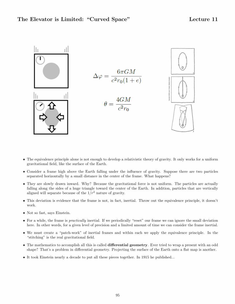
The Elevator is Limited: “Curved Space” Lecture 11

� The equivalence principle alone is not enough to develop a relativistic theory of gravity. It only works for a uniformgravitational field, like the surface of the Earth.

� Consider a frame high above the Earth falling under the influence of gravity. Suppose there are two particlesseparated horizontally by a small distance in the center of the frame. What happens?

� They are slowly drawn inward. Why? Because the gravitational force is not uniform. The particles are actuallyfalling along the sides of a huge triangle toward the center of the Earth. In addition, particles that are verticallyaligned will separate because of the 1/r2 nature of gravity.

� This deviation is evidence that the frame is not, in fact, inertial. Throw out the equivalence principle, it doesn’twork.

� Not so fast, says Einstein.

� For a while, the frame is practically inertial. If we periodically “reset” our frame we can ignore the small deviationhere. In other words, for a given level of precision and a limited amount of time we can consider the frame inertial.

� We must create a “patch-work” of inertial frames and within each we apply the equivalence principle. In the“stitching” is the real gravitational field.

� The mathematics to accomplish all this is called differential geometry. Ever tried to wrap a present with an oddshape? That’s a problem in differential geometry. Projecting the surface of the Earth onto a flat map is another.

� It took Einstein nearly a decade to put all these pieces together. In 1915 he published...

95

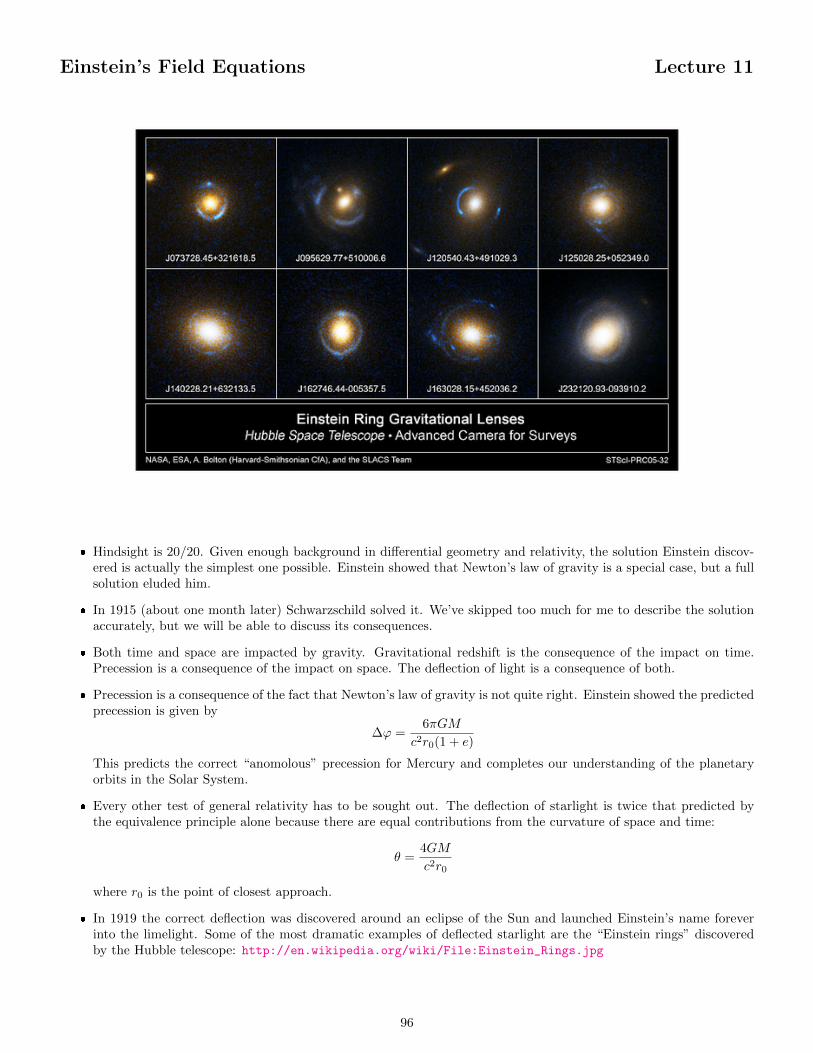
Einstein’s Field Equations Lecture 11

� Hindsight is 20/20. Given enough background in differential geometry and relativity, the solution Einstein discov-ered is actually the simplest one possible. Einstein showed that Newton’s law of gravity is a special case, but a fullsolution eluded him.

� In 1915 (about one month later) Schwarzschild solved it. We’ve skipped too much for me to describe the solutionaccurately, but we will be able to discuss its consequences.

� Both time and space are impacted by gravity. Gravitational redshift is the consequence of the impact on time.Precession is a consequence of the impact on space. The deflection of light is a consequence of both.

� Precession is a consequence of the fact that Newton’s law of gravity is not quite right. Einstein showed the predictedprecession is given by

∆ϕ =6πGM

c2r0(1 + e)

This predicts the correct “anomolous” precession for Mercury and completes our understanding of the planetaryorbits in the Solar System.

� Every other test of general relativity has to be sought out. The deflection of starlight is twice that predicted bythe equivalence principle alone because there are equal contributions from the curvature of space and time:

θ =4GM

c2r0

where r0 is the point of closest approach.

� In 1919 the correct deflection was discovered around an eclipse of the Sun and launched Einstein’s name foreverinto the limelight. Some of the most dramatic examples of deflected starlight are the “Einstein rings” discoveredby the Hubble telescope: http://en.wikipedia.org/wiki/File:Einstein_Rings.jpg

96

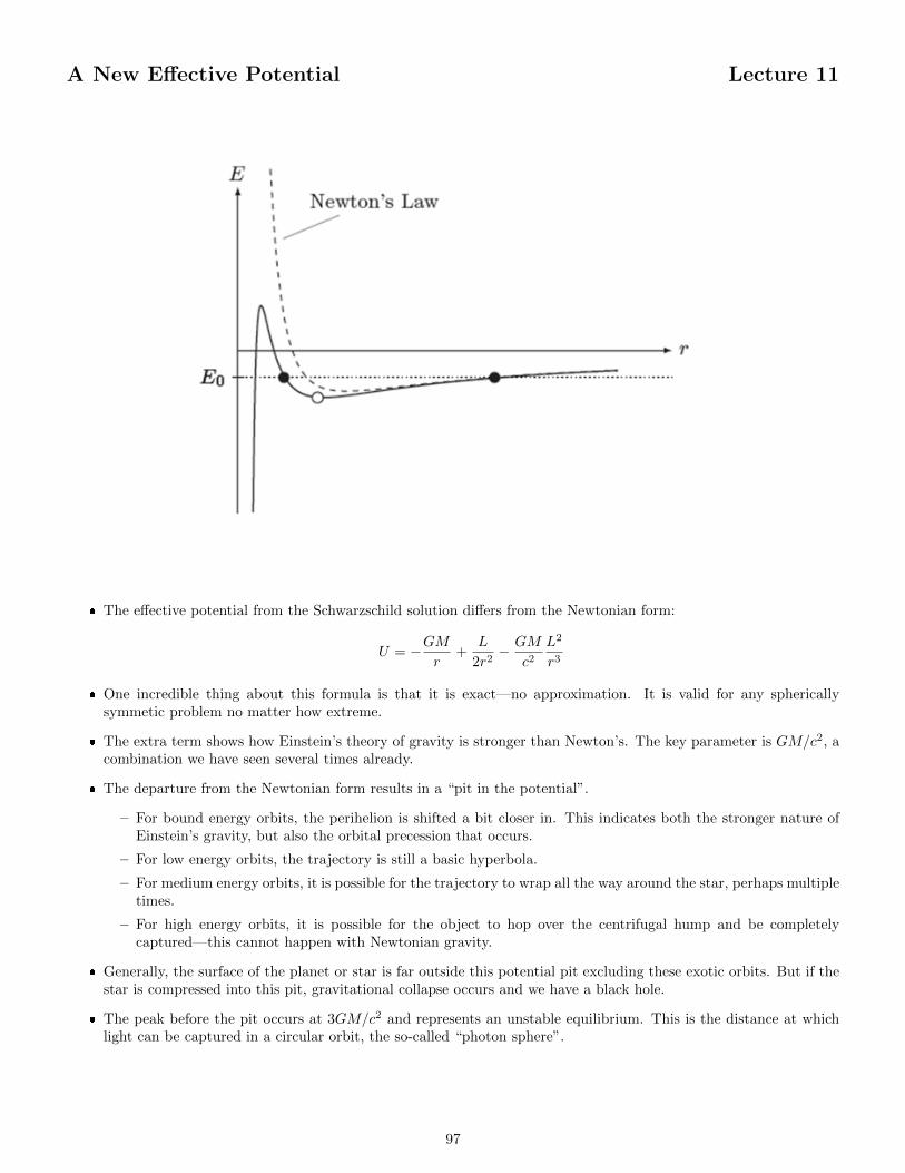
A New Effective Potential Lecture 11

� The effective potential from the Schwarzschild solution differs from the Newtonian form:

U = −GMr

+L

2r2− GM

c2L2

r3

� One incredible thing about this formula is that it is exact—no approximation. It is valid for any sphericallysymmetic problem no matter how extreme.

� The extra term shows how Einstein’s theory of gravity is stronger than Newton’s. The key parameter is GM/c2, acombination we have seen several times already.

� The departure from the Newtonian form results in a “pit in the potential”.

– For bound energy orbits, the perihelion is shifted a bit closer in. This indicates both the stronger nature ofEinstein’s gravity, but also the orbital precession that occurs.

– For low energy orbits, the trajectory is still a basic hyperbola.

– For medium energy orbits, it is possible for the trajectory to wrap all the way around the star, perhaps multipletimes.

– For high energy orbits, it is possible for the object to hop over the centrifugal hump and be completelycaptured—this cannot happen with Newtonian gravity.

� Generally, the surface of the planet or star is far outside this potential pit excluding these exotic orbits. But if thestar is compressed into this pit, gravitational collapse occurs and we have a black hole.

� The peak before the pit occurs at 3GM/c2 and represents an unstable equilibrium. This is the distance at whichlight can be captured in a circular orbit, the so-called “photon sphere”.

97

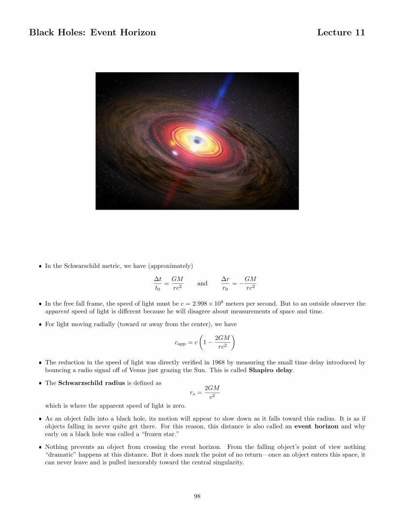
Black Holes: Event Horizon Lecture 11

� In the Schwarschild metric, we have (approximately)

∆t

t0=GM

rc2and

∆r

r0= −GM

rc2

� In the free fall frame, the speed of light must be c = 2.998× 108 meters per second. But to an outside observer theapparent speed of light is different because he will disagree about measurements of space and time.

� For light moving radially (toward or away from the center), we have

capp = c

(1− 2GM

rc2

)� The reduction in the speed of light was directly verified in 1968 by measuring the small time delay introduced by

bouncing a radio signal off of Venus just grazing the Sun. This is called Shapiro delay.

� The Schwarzschild radius is defined as

rs =2GM

c2

which is where the apparent speed of light is zero.

� As an object falls into a black hole, its motion will appear to slow down as it falls toward this radius. It is as ifobjects falling in never quite get there. For this reason, this distance is also called an event horizon and whyearly on a black hole was called a “frozen star.”

� Nothing prevents an object from crossing the event horizon. From the falling object’s point of view nothing“dramatic” happens at this distance. But it does mark the point of no return—once an object enters this space, itcan never leave and is pulled inexorably toward the central singularity.

98

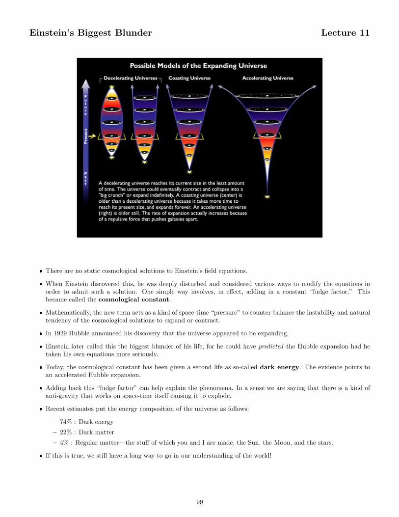
Einstein’s Biggest Blunder Lecture 11

� There are no static cosmological solutions to Einstein’s field equations.

� When Einstein discovered this, he was deeply disturbed and considered various ways to modify the equations inorder to admit such a solution. One simple way involves, in effect, adding in a constant “fudge factor.” Thisbecame called the cosmological constant.

� Mathematically, the new term acts as a kind of space-time “pressure” to counter-balance the instability and naturaltendency of the cosmological solutions to expand or contract.

� In 1929 Hubble announced his discovery that the universe appeared to be expanding.

� Einstein later called this the biggest blunder of his life, for he could have predicted the Hubble expansion had hetaken his own equations more seriously.

� Today, the cosmological constant has been given a second life as so-called dark energy. The evidence points toan accelerated Hubble expansion.

� Adding back this “fudge factor” can help explain the phenomena. In a sense we are saying that there is a kind ofanti-gravity that works on space-time itself causing it to explode.

� Recent estimates put the energy composition of the universe as follows:

– 74% : Dark energy

– 22% : Dark matter

– 4% : Regular matter—the stuff of which you and I are made, the Sun, the Moon, and the stars.

� If this is true, we still have a long way to go in our understanding of the world!

99

Index

acceleration, 9angular acceleration, 49, 58angular displacement, 49, 58angular momentum, 50, 59angular velocity, 49, 58aphelion, 84average, 7

basis, 23binomial theorem, 8

center of mass, 77central, 83centrifugal force, 41centripetal, 38centripetal force, 39coefficient of restitution, 76completely inelastic, 76conservation of energy, 70continuous, 8Coriolis force, 41cosmological constant, 99cross product, 27

dark energy, 99degrees of freedom, 51, 60delta-v, 87differential geometry, 95displacement, 6dot product, 27dynamic balancing, 54, 63

eccentricity, 84effective potential, 85elastic collision, 76energy, 67escape velocity, 89Euler-Lagrange equations, 51, 60event horizon, 98excess velocity, 89

Feynman diagrams, 81forbidden regions, 72four-vectors, 27free rotation, 53, 62free-body diagram, 31

generalized coordinates, 51, 60gravitational redshift, 93gravitational slingshot, 88gyroscopic precession, 54, 63

Hohmann transfer orbit, 87

ideal gas, 81ideal pulley, 33ideal rope, 33impact parameter, 78impetus, 16impulse, 74inertial forces, 41instantaneous, 7

joule, 66

kilogram, 5, 30kinetic energy, 68kinetic equilibrium, 21kinetic friction, 35

lab frame, 77law of gravity, 42lever arm, 47, 56limit, 7line of action, 47, 56long-range, 36

major axis, 84mechanical advantage, 65mechanics, 3meter, 5moment of inertia, 50, 59

normal, 34nutation, 54, 63

orientation, 49, 58

particle, 4perihelion, 84period, 38perturbation, 45potential energy, 69power, 66precession, 45principal axes, 53, 62principle of relativity, 32

radians, 49, 58radius of curvature, 40radius of gyration, 50, 59reduced mass, 79reference frame, 6

100

rigid body, 46, 55rocket equation, 88

Schwarzschild radius, 98second, 5semi-latus rectum, 89Shapiro delay, 98simple machines, 65speed, 6static equilibrium, 21static friction, 35statistical mechanics, 81system, 67

tensors, 27terminal velocity, 14time dilation, 94trajectory, 17turning points, 72

unbound, 89unit vector, 26

velocity, 6

watt, 66work, 66

101