INTRODUCING THE CHAINED CONSUMER PRICE INDEX

Robert Cage, John Greenlees, and Patrick Jackman U.S. Bureau of Labor Statistics

To be presented at the Seventh Meeting of the International Working Group on Price Indices

Paris, France, May 2003

The authors would like to thank Ralph Bradley, David Scott Johnson, Joshua Klick, and Cassandra Wirth for helpful comments and suggestions on this paper. They also thank the organizers of and participants in seminars on the Chained CPI at the Federal Reserve Banks of New York, Philadelphia, Dallas, Atlanta, San Francisco, Chicago, St. Louis, and Richmond. Particular thanks are also due to Erwin Diewert for his insights on superlative index design problems, without assigning him any responsibility for the choices ultimately made for the C-CPI-U. Finally, credit for many of the analyses reported in the paper goes to the Superlative Design Team of the Bureau of Labor Statistics: Ralph Bradley, Robert Cage, Alan Dorfman, Dennis Fixler, Richard Kerr, Janice Lent, Robert McClelland, Gary McMullin, and Janet Williams.

- ii -

Abstract

Introducing the Chained Consumer Price Index

Robert Cage, John Greenlees, and Patrick Jackman

In August 2002, the U.S. Bureau of Labor Statistics began publishing a

consumer price index (CPI) called the Chained Consumer Price Index for All Urban

Consumers. Designated the C-CPI-U, the index employs a superlative Tornqvist

formula and utilizes expenditure data in adjacent time periods in order to reflect the

effect of any substitution that consumers make across item categories in response to

changes in relative prices. The new measure is designed to be a closer approximation

to a "cost-of- living" index than the existing BLS measures.

Expenditure data required for the calculation of the C-CPI-U are available only

with a time lag. Thus, monthly values of the C-CPI-U are issued first in preliminary

form using the latest available expenditure data and are subject to two subsequent

revisions. Accordingly, at the time of its introduction in August 2002, "Final" values

of the C-CPI-U were issued for the 12 months of 2000, "Interim" values were issued

for the 12 months of 2001, and "Initial" values were issued for January-July of 2002.

In February 2003, with release of the January 2003 index, revised Interim indexes

for the 12 months of 2002 were published, and the index values for 2001 were

revised and became Final.

This paper details the calculation of the C-CPI-U and discusses the issues that

were addressed in its design. The paper also describes the differences between the

new index and the existing Laspeyres-formula CPI-U, and the February 2003 data

revisions.

- iii -

TABLE OF CONTENTS PAGE I. INTRODUCTION ......................................................................... 1 II. CONCEPTUAL FRAMEWORK ........................................................... 1 III. ESTIMATION METHODOLOGY ....................................................... 6

A. Construction of the Consumer Price Index ................................ 8

B. Availability of requisite expenditure data .................................. 10

C. Estimation of upper-level price change ..................................... 11

Input elementary price indexes ............................................ 11

Input elementary expenditure weights .................................. 13

a. CPI-U ................................................................. 14

b. Final C-CPI-U ...................................................... 17

c. Initial and Interim CPI-U ....................................... 18

Aggregation formula ............................................................ 19

a. CPI-U ................................................................. 19

b. Final C-CPI-U ...................................................... 20

c. Initial and Interim CPI-U ....................................... 21

IV. COMPARING AND CONTRASTING C-CPI-U VERSIONS ................... 28

A. Difference in estimation ......................................................... 28

V. COMPARING AND CONTRASTING THE C-CPI-U AND THE CPI-U..... 30

A. Difference in estimation ......................................................... 30

B. Index simulations .................................................................. 30

VI. INAUGURAL PUBLISHED INDEXES ............................................... 33

VII. 2003 REVISIONS AND MOST CURRENT PUBLISHED INDEXES ...... 33

Comparisons with Personal Consumption Expenditure Indexes ......... 35

VIII SUMMARY AND DIRECTIONS OF FURTHER RESEARCH .................. 35

TABLES AND FIGURES ......................................................................... 39

I. INTRODUCTION

In August 2002, the U.S. Bureau of Labor Statistics (BLS) began publishing a

new index of consumer price change called the Chained Consumer Price Index for All

Urban Consumers. Designated the C-CPI-U, the index supplements the existing

indexes already produced by the BLS: the CPI for All Urban Consumers (CPI-U) and

the CPI for Urban Wage Earners and Clerical Workers (CPI-W). The BLS is producing

the C-CPI-U in order to address a perceived weakness of the CPI-U: upper-level

substitution bias. By utilizing a superlative price index aggregator across items, the

C-CPI-U is designed to be a closer approximation to a “cost-of-living” index (COLI)

than the CPI-U and the CPI-W.

This paper provides comprehensive information on concepts, definitions,

statistical procedures, and estimation methods used by BLS to compile the C-CPI-U.

Because the primary motivation behind publishing the C-CPI-U is to provide data

users an index that more closely approximates a COLI, the paper begins with a brief

summary of cost-of-living and consumer substitution theory. A cursory review of

prior research on the substitution bias inherent in the CPI-U is also provided. Next, a

detailed explanation of how BLS computes the C-CPI-U is outlined in a step-by-step

fashion. Estimation methodologies for the C-CPI-U and CPI-U are then compared and

contrasted, and differences between the two indexes are evaluated. Finally, because

price indexes can be used for many purposes and indexes well-suited for one

purpose may be ill-suited for another, the limitations of the C-CPI-U are identified so

that users may evaluate the suitability of the index for their needs.

II. CONCEPTUAL FRAMEWORK

The Consumer Price Index is a measure of the average price change of a fixed

market basket of goods and services purchased by the average urban household in

- 2 -

the United States. The market basket consists of a sample of items – food, clothing,

shelter, fuels, and other goods and services –that consumers buy for day-to-day

living. Price change is measured by repricing essentially the same market basket of

goods and services at regular intervals and comparing aggregate costs with the costs

of the same market basket in an arbitrarily selected base period.

BLS calculates a CPI for two population groups: (1) urban wage-earners and

clerical workers and (2) all urban consumers. The Consumer Price Index for Urban

Wage Earners and Clerical Workers (CPI-W) is a continuation of the historical index

introduced by BLS in the early 1900’s for use in wage negotiations.1 The Consumer

Price Index for All Urban Consumers (CPI-U) was introduced in 1978 as a broader

and more representative index of the urban, non-institutional population of the

United States. Because the same basic methodology is used for calculating both the

CPI-W and CPI—U, the discussion in this paper focuses on the relationship between

the CPI-U and the new superlative index.

Over the past 80 years, the methodology for producing both CPI’s has been

refined by way of improvements in price data collection techniques, adjustments in

estimation methods, and continuous surveys of consumer spending behavior.

Comprehensive revisions to the CPI have occurred in 1940, 1953, 1964, 1978, 1987,

and 1998.2 Other improvements have been made over the years that reflect not

only BLS’s own experience and research, but also the criticisms and

recommendations of outsiders.3 The goal of each improvement has been to

effectuate in the index a more accurate representation of contemporaneous buying

habits and consumption costs. A unifying framework for dealing with practical

1 See U.S. Department of Labor, BLS Handbook of Methods, Bulletin 2490, 1997, Chapter 17: The Consumer Price Index, p.167. 2 For an overview of historical CPI revisions, see John S. Greenlees and Charles C. Mason, “Overview of the 1998 revision of the Consumer Price Index.” Monthly Labor Review, December 1996, pp. 3-9. 3 For an early example, see, Report of The President’s Committee on the Cost of Living (Washington, Office of Economic Stabilization, 1945).

- 3 -

questions that arise in the construction of the CPI, in assessment of the CPI’s quality,

and in guiding improvements made to the index, has been the economic approach to

index numbers and, specifically, the concept of the cost-of-living index (COLI).

While the use of index numbers to measure price change dates back to 1707,

the economic theory of index numbers is of much more recent vintage.4 The theory

underlying the COLI was developed by A. A. Konus in 1924.5 Under the assumption

of utility maximizing behavior, a COLI is defined as the ratio of the minimum

expenditure required to attain a particular level of satisfaction in two price situations,

a comparison period and a base period. The CPI-U and the CPI-W are modified

Laspeyres indexes that hold the standard of living constant in the span between

major revisions by keeping quantities fixed at the level consumed in the base period,

but allowing prices to vary. The restriction imposed on these CPI’s - holding the

quantities fixed and not allowing substitution among goods in response to relative

price change - results in a divergence between the CPI (or any other index with fixed

quantity weights) and the COLI. In the case of a Laspeyres index, the effect is such

that it is greater than or equal to the true cost of living. Indeed, it is well known that

a Laspeyres index is an upper bound to the true COLI.6 In analyses of the CPI by

outside reviewers, it often has been argued that the BLS should establish a cost-of-

living index as the objective in measuring consumer prices.7 The BLS has long said

that it operates within a COLI framework in producing the CPI.8 There are, of

4 The first quantitative study of price levels was apparently made by Bishop Fleetwood in Chronicon-Preciosum in 1707. For a historical survey of price measurement, see W. Erwin Diewert, “The Early History of Price Index Research,” W. Erwin Diewert and A.O. Nakamura (eds.), Essays in Index Number Theory, Volume I, 1993. 5 “The Problem of the True Index of the Cost of Living,” English translation of the original in Russian published in 1939 in Econometrica 7, pp. 10-29. 6 In general, a Laspeyres index is only an upper bound to a COLI when comparing the “comparison” period with the “base” period, not with an intermediate period. 7 See, for example, The Price Statistics of the Federal Government, prepared by the Price Statistics Review Committee of the National Bureau of Economic Research, 1961, the Final Report of the Advisory Commission to Study the Consumer Price Index, submitted to the Committee on Finance, U.S. Senate, 1996, and Charles Schultze and Chris Mackie (eds.), At What Price? Conceptualizing and Measuring Cost-of-Living and Price Indexes, 2002. 8 See, Robert F. Gillingham, “A Conceptual Framework for the Consumer Price Index,” Proceedings, Business and Economics Statistics Section, American Statistical Association, 1974, pp. 246-52, and John S. Greenlees, “The U.S. CPI

- 4 -

course, a number of differences between the CPI and a complete COLI other than the

ability to reflect how consumers adjust their consumption to changes in relative

prices. For example, the CPI ignores the fact that household preferences extend to

choices between labor and leisure and among different types of leisure. It also

ignores time by assuming that all consumption takes place in a single period. It

generally ignores the impact of both the environment and government goods on

household welfare. Reflection of substitution in response to changes in relative

prices is, therefore, only part of what is required for a complete COLI. It is,

however, that aspect of a COLI that has been the focus of the technical criticism of

the CPI. The recent study by the Committee on National Statistics stated that:

“Within the general conceptual framework of cost-of-living indexes, the appropriate

theoretical concept for the CPI is a conditional cost-of-living index that is restricted

to private goods and services and in which environmental background factors are

held constant.”9

The theory underlying the C-CPI-U was based largely on the work of W. Erwin

Diewert, who demonstrated that a family of indexes, termed superlative, could be

calculated that provided a close approximation to a COLI using only the observable

price and quantity data.10 That is, it would not be necessary to econometrically

estimate the elasticities of substitution of all of the items with each other. The most

widely known index number formulas that belong to the superlative class identified

by Diewert are the Fisher Ideal index and the Tornqvist index. The Fisher Ideal

Index is a geometric average of a base-period-weighted Laspeyres index and a

current-period-weighted Paasche index. The Tornqvist index utilizes expenditure

and the Cost-of-Living Objective,” presented at the Joint ECE/ILO Meeting on Consumer Price Indices in Geneva, Switzerland, November 2, 2001. 9 Schultze and Mackie, At What Price?, p. 73. 10 See, W. Erwin Diewert, “Exact and Superlative Index Numbers,” Journal of Econometrics 4, pp. 114-45, 1976. By a close approximation, Diewert states that the functional form for the price index is “superlative” if it is exact for a function that can provide a second order approximation to an arbitrary twice differentiable linearly homogenous function.

- 5 -

data in both the current and base time periods in order to reflect the effect of any

substitution that consumers may make across item categories in response to

changes in relative prices. Hence, both indexes arrive at an estimate of average

price change over two time periods by utilizing in some fashion the expenditure

experience in both periods as weights.

Although funds were initially appropriated in 1998, the development of the C-

CPI-U has its roots back at least as far as 1961, with the recommendation from the

Price Statistics Review Committee, known as the Stigler Committee, that a constant

utility index is the appropriate index for the main purposes of the CPI.11 At the same

time, the Stigler Committee recognized the need to fund research organizations

within the price collection agencies to deal with price and index number issues

outside of a production framework. Following the formation of BLS’s Division of Price

and Index Number Research in 1966, research on developing a COLI was instituted.

Much of the theoretical work on the COLI was done by Robert Pollak, first working at

BLS on sabbatical from the University of Pennsylvania and later as a consultant.12

On an empirical side, several studies have examined the extent of the substitution

effect between a Laspeyres measure and the COLI. On an aggregate level, these

include studies by Steven D. Braithwait,13 Marilyn E. Manser and Richard J.

McDonald,14 and Ana A. Aizcorbe and Patrick C. Jackman.15 Braithwait utilized

annual price and quantity data on Personal Consumption Expenditures from the

National Income and Product Accounts for 53 commodities and found that for the

fifteen year period 1958-73, the Laspeyres index overstated the COLI by 1.5

percent, or about 0.1 percent a year. The work by Manser and McDonald covered

11 The Price Statistics of the Federal Government, p. 52. 12 See Robert A. Pollak, The Theory of the Cost-of-Living Index. New York: Oxford University Press, 1989. 13 Steven D. Braithwait, “Substitution Bias of the Laspeyres Price Index: An Analysis Using Estimated Cost-of Living Indexes,” American Economic Review, March 1980, pp.64-77. 14 Marilyn E. Manser and Richard J. McDonald, “An Analysis of Substitution Bias in Measuring Inflation, 1959-85,” Econometrica, July 1988, pp.909-30.

- 6 -

the period from 1959-85 and utilized data on Personal Consumption Expenditures for

101 commodities. On an annual basis this resulted in an estimate of the substitution

effect of .19 percent per year. In addition to the numerical estimate of substitution

effect, the Manser-McDonald study established the upper and lower bounds for the

amount of substitution effect in the Laspeyres index - between .14 and .22 percent

per year in the 1959-1985 period. The Aizcorbe-Jackman study examined the

substitution effect issue using detailed expenditure data from the Consumer

Expenditure (CE) Surveys, the official source used for the CPI. Consumer

Expenditure data include a finer level of disaggregation in the commodity classes as

well as geographic detail than do data from the Bureau of Economic Analysis. At that

time, there were 207 item categories and 44 areas, which allowed the different

formulas to be applied at a lower level of aggregation than the earlier studies.

Aizcorbe-Jackman’s estimate of the substitution effect for the period from 1982

through 1991 was .20 or .27 percent per annum, depending on whether a fixed base

or chained index was used.

III. ESTIMATION METHODOLOGY

Specification and development of an official superlative index presented many

challenges for the BLS. Foremost among these were the issues surrounding the

sampling errors in CPI price and expenditure data. In most theoretical discussions of

superlative indexes, price indexes and expenditure shares are taken as known with

certainty, as if the data reflected a single representative consumer who allocates his

or her spending in response to the observed price indexes. The CPI pricing surveys

and the Consumer Expenditure Survey, however, are based on finite and distinct

15 Ana A. Aizcorbe and Patrick C. Jackman, “The Commodity Substitution Effect in CPI Data, 1982-91,” Monthly Labor Review, December 1993, pps 25-33.

- 7 -

samples of outlets and consumers, respectively. Sample sizes are especially small at

the level of basic item-area indexes and weights, such as were used in the Aizcorbe-

Jackman work discussed above. The existence of sampling variation in the

underlying CPI data, and the independence of the sampling errors in price indexes

and expenditure shares, can affect the expectation of a superlative index computed

from those data.16

The impact of sampling variance could have been mitigated by constructing

the C-CPI-U using only national-level data, but this would have tended to

underestimate the true substitution effect.17 Alternatively, the BLS could have

chosen to produce only an annual C-CPI-U, using price and expenditure data

averaged over the year. 18 This option was also rejected, on the basis that the

usefulness of the index would have been sharply reduced if it were not made

available on a monthly basis.

It was also determined that, rather than publishing the C-CPI-U only with a

lag, the BLS would publish the index in preliminary form and revise it when more

timely expenditure data were received and processed. As with the decision to

produce a monthly C-CPI-U, this decision was motivated in part by an expectation

that some users would desire a monthly, timely superlative index and would

estimate such indexes themselves if the BLS did not publish the C-CPI-U in that

form.

The BLS was thus faced with the problem of choosing how to employ volatile

price and expenditure data from small samples to compute a monthly superlative

series. After much discussion, it was further decided to chain the monthly index

16 For a discussion of these issues see John S. Greenlees, "Random Errors and Superlative Indexes," Bureau of Labor Statistics Working Paper 343, March 2001, or A.H. Dorfman, S.G. Leaver, and J. Lent, “Some Observations on Price Index Estimators,” Proceedings of the Federal Committee on Statistical Methodology Research Conference, Monday B Sessions, pp. 56-65, 1999. 17 See Greenlees, op. cit.

- 8 -

values, despite the volatile and potentially seasonal nature of the underlying data,

rather than attempting to impose chaining on an annual or other frequency. Many of

the specific design features described below reflect difficult choices made among

several imperfect alternatives, without the benefit of guidance from index number

theory. Fortunately, analyses of historical data indicated that simulated C-CPI-U

series were surprisingly robust to their specific design features, particularly at the

aggregate level.

A second significant issue was determining how to compute the preliminary C-

CPI-U indexes, which could not use a true superlative formula. The objective was to

develop a specification that would yield accurate forecasts of the Final C-CPI-U.

Again, a variety of alternative formulas were evaluated, but simulation studies

showed that the differences in the resulting preliminary index values were relatively

small.

A. Construction of the Consumer Price Index

The CPI is built in two stages. In the first stage, price changes for roughly

80,000 specific items per month are averaged to yield 8,018 estimates of aggregate

price change. This stage is often referred to as “lower-level aggregation” or

“elementary-level aggregation” as it involves averaging the most fundamental

component of the index - observed price change for specifically defined consumer

goods, services, and products.19 For example, the prices of approximately ten

different brands and styles of watches at various locations in Chicago are observed

each month, compared to the prices observed in the previous month, and averaged

together to produce an index of price change for watches in Chicago. Watches

(ITEM=AG01) is one of 211 elementary items, and Chicago (AREA=A207) is one of

18 Erwin Diewert, “Notes on Producing an Annual Superlative Index Using Monthly Price Data,” University of British Columbia Economics Department Discussion Paper No. 00-08 (July 2000) discusses issues in constructing an annual superlative index.

- 9 -

38 elementary areas in the current CPI market basket structure. The Chicago-watch

index is one of the 8,018 (211 items x 38 areas) elementary indexes produced in the

first stage of CPI construction.

In the second stage, the elementary indexes are averaged together to yield

various aggregate indexes and ultimately the All-Items, U.S. City Average index of

price change. See Figure 3.1.

Within the two-tiered scheme of calculating the CPI, consumer substitution

can and does occur at both levels. Ideally, a superlative formula would be employed

at both stages of CPI index construction to account for consumer substitution that

might occur intra-item, that is among specific products within an elementary item

(e.g., a leather band watch versus a stainless steel band watch or whole wheat bread

versus white bread) and inter-item, that is across elementary items (e.g., theater

admission versus video rental or beer versus wine). However, the BLS is currently

precluded from using a superlative formula at the first stage because reliable

monthly expenditure data for each of the 80,000 lower-level quotes are not readily

ascertainable.20 As an alternative to a superlative index as a means of addressing

intra-item substitution, the BLS began using a hybrid combination of Geometric Mean

indexes and Laspeyres indexes for lower-level aggregation in 1999.21 Zero elasticity

of substitution within item categories is assumed for the small number of item

categories in which the Laspeyres formula is used.22 Unitary elasticity of substitution

intra-item is assumed for items using the Geometric Mean formula.

19 In BLS terminology, the specific goods and services at the lower-level are called price quotes. 20 Collecting monthly information from CPI outlets on the sales of individual items would be extremely costly and would impose an unacceptable respondent burden. 21 For more information on the use of the Geometric Mean index in lower-level CPI aggregation CPI, see Kenneth V. Dalton, John S. Greenlees, and Kenneth J. Stewart: “Incorporating a geometric mean formula into the CPI,” Monthly Labor Review, October, 3-7, 1998. 22 Laspeyres items are Local telephone service, Rent, Housing at school, Owners’ equivalent rent, Electricity, Natural gas, Water and sewerage service, Physicians’ services, Dental services, Eyeglasses and eye care, Other medical professional service, Hospital services, Nursing homes and adult daycare, Cable television, and State and local vehicle registration, license, and motor vehicle property tax.

- 10 -

The use of a superlative formula for upper-level aggregation is designed to

address inter-item substitution. In order to use a superlative index formula at the

upper-level, monthly expenditure estimates for each of the 8,018 elementary item-

area combinations are required. Expenditure weights for CPI upper-level

aggregation are derived from the Consumer Expenditure Surveys.23 Effective with

data collected in 1999, the CE sample size was increased by 50 percent, in part to

accommodate production of the C-CPI-U.

B. Availability of Requisite Expenditure Data

Consumer Expenditure Survey data are processed annually and made

available for CPI use with a substantial lag. For example, data for calendar year

2001 were not available until the fourth quarter of 2002. Data for calendar year 2002

will not be available until the fourth quarter of 2003. This lag in data availability

prevents BLS from calculating and publishing a superlative index in real time, i.e., on

the same contemporaneous publication schedule as the CPI-U. BLS could have

opted to simply calculate and publish the C-CPI-U on a two-year lag schedule. For

example, superlative indexes for all months of calendar year 2002 could have been

released in early 2004. However, as noted above, demand for the superlative

indexes concomitant with the release of the CPI-U was anticipated to be high.

Therefore, BLS developed the following general estimation and publication schedule

for the C-CPI-U index for a given month (t) in year (y):

�� Following Month (t+1): Calculate and publish an Initial estimate of the month (t) superlative index using lagged expenditure data

�� February of Following Year (y+1): Revise and publish each Initial monthly superlative index from year (y) with an Interim estimate based upon updated, but still lagged expenditure data

23 The Consumer Expenditure Surveys have been conducted continuously since 1980 by the U.S. Bureau of the Census under contract with the BLS.

- 11 -

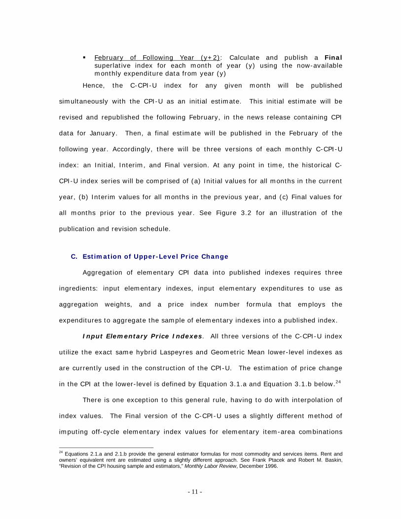
�� February of Following Year (y+2): Calculate and publish a Final superlative index for each month of year (y) using the now-available monthly expenditure data from year (y)

Hence, the C-CPI-U index for any given month will be published

simultaneously with the CPI-U as an initial estimate. This initial estimate will be

revised and republished the following February, in the news release containing CPI

data for January. Then, a final estimate will be published in the February of the

following year. Accordingly, there will be three versions of each monthly C-CPI-U

index: an Initial, Interim, and Final version. At any point in time, the historical C-

CPI-U index series will be comprised of (a) Initial values for all months in the current

year, (b) Interim values for all months in the previous year, and (c) Final values for

all months prior to the previous year. See Figure 3.2 for an illustration of the

publication and revision schedule.

C. Estimation of Upper-Level Price Change

Aggregation of elementary CPI data into published indexes requires three

ingredients: input elementary indexes, input elementary expenditures to use as

aggregation weights, and a price index number formula that employs the

expenditures to aggregate the sample of elementary indexes into a published index.

Input Elementary Price Indexes. All three versions of the C-CPI-U index

utilize the exact same hybrid Laspeyres and Geometric Mean lower-level indexes as

are currently used in the construction of the CPI-U. The estimation of price change

in the CPI at the lower-level is defined by Equation 3.1.a and Equation 3.1.b below.24

There is one exception to this general rule, having to do with interpolation of

index values. The Final version of the C-CPI-U uses a slightly different method of

imputing off-cycle elementary index values for elementary item-area combinations

24 Equations 2.1.a and 2.1.b provide the general estimator formulas for most commodity and services items. Rent and owners’ equivalent rent are estimated using a slightly different approach. See Frank Ptacek and Robert M. Baskin, “Revision of the CPI housing sample and estimators,” Monthly Labor Review, December 1996.

- 12 -

priced on a bimonthly schedule.25 In the CPI-U, off-cycle bimonthly elementary

indexes are set equal to the previous-month index value.26

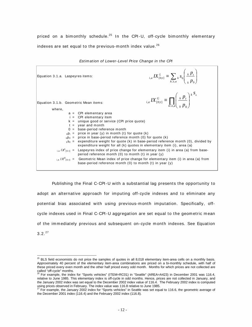
Estimation of Lower-Level Price Change in the CPI

Equation 3.1.a. Laspeyres items:

Equation 3.1.b. Geometric Mean items:

where, a = CPI elementary area

i = CPI elementary item k = unique good or service (CPI price quote)

t = year and month 0 = base-period reference month

kpt = price in year (y) in month (t) for quote (k) kp0 = price in base-period reference month (0) for quote (k)

ks0 = expenditure weight for quote (k) in base-period reference month (0), divided by expenditure weight for all (k) quotes in elementary item (i), area (a)

i,a IXL[0;t] = Laspeyres index of price change for elementary item (i) in area (a) from base-

period reference month (0) to month (t) in year (y)

i,a IXG[0;t] = Geometric Mean index of price change for elementary item (i) in area (a) from

base-period reference month (0) to month (t) in year (y)

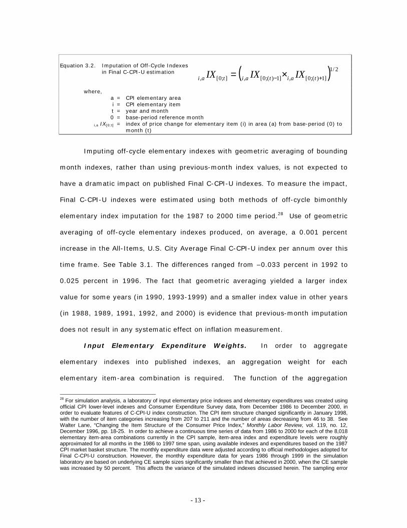
Publishing the Final C-CPI-U with a substantial lag presents the opportunity to

adopt an alternative approach for imputing off-cycle indexes and to eliminate any

potential bias associated with using previous-month imputation. Specifically, off-

cycle indexes used in Final C-CPI-U aggregation are set equal to the geometric mean

of the immediately previous and subsequent on-cycle month indexes. See Equation

3.2.27

25 BLS field economists do not price the samples of quotes in all 8,018 elementary item-area cells on a monthly basis. Approximately 40 percent of the elementary item-area combinations are priced on a bi-monthly schedule, with half of these priced every even month and the other half priced every odd month. Months for which prices are not collected are called “off-cycle” months. 26 For example, the index for “Sports vehicles” (ITEM=RC01) in “Seattle” (AREA=A423) in December 2001 was 116.4, relative to June 1985. This elementary index is off-cycle in odd months. Hence, prices are not collected in January, and the January 2002 index was set equal to the December 2002 index value of 116.4. The February 2002 index is computed using prices observed in February. The index value was 116.8 relative to June 1985. 27 For example, the January 2002 index for “Sports vehicles” in Seattle was set equal to 116.6, the geometric average of the December 2001 index (116.4) and the February 2002 index (116.8).

�∈

��

�

�

��

�

�=

aik k

k tk

Ltai p

psIX

, 00];0[,

∏∈

��

�

�

��

�

�=

aik

k

k

k tGtai

s

pp

IX, 0

];0[,

0

- 13 -

( ) 2/1]1)(;0[,]1)(;0[,];0[, +− ×= taitaitai IXIXIX

Equation 3.2. Imputation of Off-Cycle Indexes in Final C-CPI-U estimation

where,

a = CPI elementary area i = CPI elementary item

t = year and month 0 = base-period reference month

i,a IX[0;t] = index of price change for elementary item (i) in area (a) from base-period (0) to month (t)

Imputing off-cycle elementary indexes with geometric averaging of bounding

month indexes, rather than using previous-month index values, is not expected to

have a dramatic impact on published Final C-CPI-U indexes. To measure the impact,

Final C-CPI-U indexes were estimated using both methods of off-cycle bimonthly

elementary index imputation for the 1987 to 2000 time period.28 Use of geometric

averaging of off-cycle elementary indexes produced, on average, a 0.001 percent

increase in the All-Items, U.S. City Average Final C-CPI-U index per annum over this

time frame. See Table 3.1. The differences ranged from –0.033 percent in 1992 to

0.025 percent in 1996. The fact that geometric averaging yielded a larger index

value for some years (in 1990, 1993-1999) and a smaller index value in other years

(in 1988, 1989, 1991, 1992, and 2000) is evidence that previous-month imputation

does not result in any systematic effect on inflation measurement.

Input Elementary Expenditure Weights. In order to aggregate

elementary indexes into published indexes, an aggregation weight for each

elementary item-area combination is required. The function of the aggregation

28 For simulation analysis, a laboratory of input elementary price indexes and elementary expenditures was created using official CPI lower-level indexes and Consumer Expenditure Survey data, from December 1986 to December 2000, in order to evaluate features of C-CPI-U index construction. The CPI item structure changed significantly in January 1998, with the number of item categories increasing from 207 to 211 and the number of areas decreasing from 46 to 38. See Walter Lane, “Changing the Item Structure of the Consumer Price Index,” Monthly Labor Review, vol. 119, no. 12, December 1996, pp. 18-25. In order to achieve a continuous time series of data from 1986 to 2000 for each of the 8,018 elementary item-area combinations currently in the CPI sample, item-area index and expenditure levels were roughly approximated for all months in the 1986 to 1997 time span, using available indexes and expenditures based on the 1987 CPI market basket structure. The monthly expenditure data were adjusted according to official methodologies adopted for Final C-CPI-U construction. However, the monthly expenditure data for years 1986 through 1999 in the simulation laboratory are based on underlying CE sample sizes significantly smaller than that achieved in 2000, when the CE sample was increased by 50 percent. This affects the variance of the simulated indexes discussed herein. The sampling error

- 14 -

weight is to assign each elementary index a relative importance or contribution in

the resulting aggregate index. The aggregation weight corresponds to consumer

tastes and preferences and resulting expenditure choices among the 211 items in the

38 areas comprising the CPI sample, for a specified time period, by the population

the index is designed to represent. This section compares the estimation and use of

aggregation weights in the Laspeyres CPI-U, preliminary C-CPI-U series, and the

Final C-CPI-U.

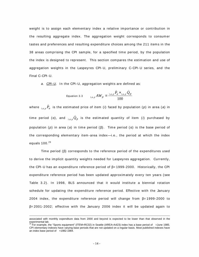
a. CPI-U. In the CPI-U, aggregation weights are defined as:

Equation 3.3 100

,,,,,,

βαβ

QPAW paipai

pai

��

×=

where αPpai

�

,, is the estimated price of item (i) faced by population (p) in area (a) in

time period (α), and βQpai

�

,, is the estimated quantity of item (i) purchased by

population (p) in area (a) in time period (β). Time period (α) is the base period of

the corresponding elementary item-area index—i.e., the period at which the index

equals 100.29

Time period (β) corresponds to the reference period of the expenditures used

to derive the implicit quantity weights needed for Laspeyres aggregation. Currently,

the CPI-U has an expenditure reference period of β=1999-2000. Historically, the CPI

expenditure reference period has been updated approximately every ten years (see

Table 3.2). In 1998, BLS announced that it would institute a biennial rotation

schedule for updating the expenditure reference period. Effective with the January

2004 index, the expenditure reference period will change from β=1999-2000 to

β=2001-2002; effective with the January 2006 index it will be updated again to

associated with monthly expenditure data from 2000 and beyond is expected to be lower than that observed in the experimental lab. 29 For example, the “Sports equipment” (ITEM=RC02) in Seattle (AREA=A423) index has a base period of �=June 1985. CPI elementary indexes have varying base periods that are not updated on a regular basis. Most published indexes have an index base period of �=1982-1984.

- 15 -

2003-2004; and so forth. Note that a change in the expenditure reference period

results in a change in the implicit quantity (Q) assigned to each elementary index,

but not the implicit price component (P) of the aggregation weight (AW).

Aggregation weights for the CPI-U are derived from estimates of household

expenditures collected in the Consumer Expenditure Survey data. Despite an

increase in the CE sample size in 1999, expenditure estimates at the elementary

item-area level would be unreliable due to sampling error without the use of

statistical smoothing procedures. BLS uses two basic techniques to minimize the

variance associated with each elementary item-area base-period expenditure

estimate. First, data are pooled over an extended time period in order to build the

expenditure estimates upon an adequate sample size. The current reference period

(β) uses 24 months of data. Second, elementary item-area expenditures are

averaged, or composite-estimated, with item-regional expenditures.30 This has the

effect of lowering the variance of each elementary item-area expenditure at the

expense of biasing it toward the expenditure patterns observed in the larger

geographical area.31

The CPI-U aggregation weight for item (i) in area (a) in reference period (β) is

computed by first calculating an aggregate annual expenditure estimate, nPQai β)(, ,

for each year (βn) in reference period (β). This estimate is derived directly from

Consumer Expenditure Survey data.32 Next, the share of total area expenditure is

computed for each item in each area, for each year. Similarly, the share of total

expenditure in each major-area (m) is computed for each item for each year. A

composite-estimated share of total expenditures is computed for each item for each

30 Elementary areas area grouped into region x city-size classifications for the purpose of composite-estimation. There are four regions and two city-size classifications for a total of eight region-city-size classifications. 31 Aggregation weights for the CPI-U and CPI-W are each derived separately according to the steps outlined in the text. 32 For a detailed explanation of how aggregate expenditure estimates are computed from CE data, see BLS Handbook of Methods, Bulletin 2490, 1997, Chapter 17.

- 16 -

year by taking a weighted average of its area share and corresponding major-area

share. The weight (δ) assigned to the major-area (m) and the weight (1−δ) assigned

to the elementary area (a) is a function of the variance and covariance of each

measure.33 The resulting average share ( nsai βˆ, ) is then multiplied by the sum of all

expenditures in the elementary area in the corresponding year, to obtain a

composite-estimated item expenditure in year (βn). This estimate is in turn multiplied

by a “raking factor” which is equivalent to the ratio of unadjusted expenditures

( nPQai β)(, ) summed to the expenditure-class, major-area level, to the composite-

estimated expenditures ( nQPai β)~~(, ) summed to the expenditure-class, major-area

level. The raking factor is designed to limit the degree to which composite-estimation

can change relative expenditures among item-area cells. Next, the composite-

estimated-and-raked expenditures for each year (βn) are averaged to obtain the final

estimate of annual aggregate expenditures in reference period (β).

The CPI-U aggregation weight for each item-area combination is then derived

from the composite-estimated-and-raked expenditure estimate by first multiplying it

by the index of price change from reference period (β) to pivot-month (v).34 The

resulting product is a cost weight: an estimate of item-area expenditures in pivot-

month (v), based upon quantities purchased in reference period (β). Finally, the cost

weight is divided by the corresponding pivot-month index to obtain the aggregation

weight: an estimate of item-area expenditure based upon quantities purchased in

reference period (β) and prices of time-period (α).

33 For more information on composite-estimation, see Michael P. Cohn and John P. Sommers, “Evaluation of the Methods of Composite Estimation of Cost Weights for the CPI,” Proceedings of the Business and Economic Statistics Section, American Statistical Association, 1984. pp. 466-7. 34 The pivot-month is the first month in which expenditures from reference period (β) are used in the CPI.

- 17 -

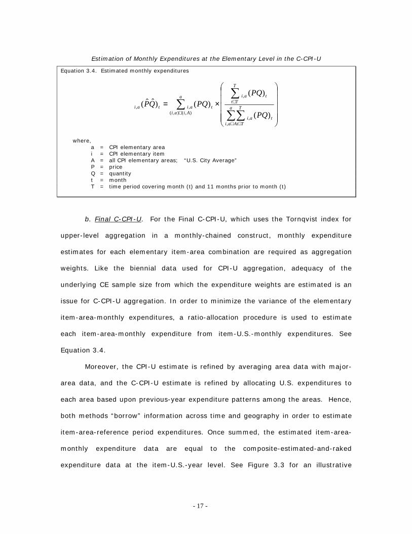
Estimation of Monthly Expenditures at the Elementary Level in the C-CPI-U

Equation 3.4. Estimated monthly expenditures

�����

�

�

�����

�

�

×=��

��

∈ ∈

∈

∈a

Aai

T

Tttai

T

Tttaia

Aiaitaitai

PQ

PQPQQP

,,

,

),(),(,,

)(

)()()ˆˆ(

where, a = CPI elementary area i = CPI elementary item A = all CPI elementary areas; “U.S. City Average” P = price Q = quantity t = month T = time period covering month (t) and 11 months prior to month (t)

b. Final C-CPI-U. For the Final C-CPI-U, which uses the Tornqvist index for

upper-level aggregation in a monthly-chained construct, monthly expenditure

estimates for each elementary item-area combination are required as aggregation

weights. Like the biennial data used for CPI-U aggregation, adequacy of the

underlying CE sample size from which the expenditure weights are estimated is an

issue for C-CPI-U aggregation. In order to minimize the variance of the elementary

item-area-monthly expenditures, a ratio-allocation procedure is used to estimate

each item-area-monthly expenditure from item-U.S.-monthly expenditures. See

Equation 3.4.

Moreover, the CPI-U estimate is refined by averaging area data with major-

area data, and the C-CPI-U estimate is refined by allocating U.S. expenditures to

each area based upon previous-year expenditure patterns among the areas. Hence,

both methods “borrow” information across time and geography in order to estimate

item-area-reference period expenditures. Once summed, the estimated item-area-

monthly expenditure data are equal to the composite-estimated-and-raked

expenditure data at the item-U.S.-year level. See Figure 3.3 for an illustrative

- 18 -

example of monthly weight estimation of an elementary item-area cell in the

C-CPI-U.

c. Initial and Interim C-CPI-U. Lacking a satisfactory method to forecast the

requisite monthly expenditure data, BLS opted to select an aggregation methodology

for the Initial and Interim versions of the C-CPI-U that would best predict the Final

C-CPI-U Tornqvist version – constrained by the use of the most contemporaneous

expenditure data available at the time of index publication, i.e., expenditures from

the CPI-U expenditure reference period (β). An adjusted Geometric Mean index

formula was ultimately adopted. See the discussion of Aggregation Formula for

Initial and Interim Indexes below.

Since the Initial version of the C-CPI-U is published simultaneously with the

CPI-U, it uses expenditure data from the same expenditure reference period (β) as

the CPI-U as aggregation weights. In contrast to the CPI-U, however, it is not

necessary to adjust the expenditures forward to a December “pivot” month and

rebase them such that the implicit price corresponds to the corresponding item-area

index base period (α). Rather, the estimated expenditure weights with implicit prices

of time period (β) and implicit quantities of time period (β) are used as aggregation

weights. This is consistent with the underlying assumption behind a geometric mean

price index aggregator: consumers respond to changing relative prices by holding

their expenditure shares constant over time. Hence, it is implicitly assumed that

each item-area expenditure share derived from reference period (β) will be equal to

each monthly item-area expenditure share over the time period in which aggregation

weights based on reference period (β) are used to construct the Initial and Interim

C-CPI-U indexes. In other words, 24,2,1,, taitaitaiai ssss ==== �β , where t1 to t24 are

the 24 months for which aggregation weights derived from (β) are used to construct

the Initial and Interim C-CPI-U indexes.

- 19 -

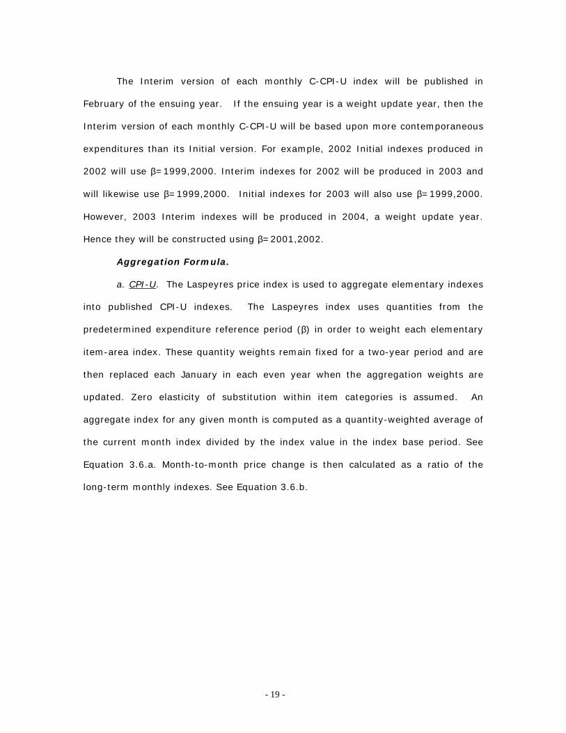
The Interim version of each monthly C-CPI-U index will be published in

February of the ensuing year. If the ensuing year is a weight update year, then the

Interim version of each monthly C-CPI-U will be based upon more contemporaneous

expenditures than its Initial version. For example, 2002 Initial indexes produced in

2002 will use β=1999,2000. Interim indexes for 2002 will be produced in 2003 and

will likewise use β=1999,2000. Initial indexes for 2003 will also use β=1999,2000.

However, 2003 Interim indexes will be produced in 2004, a weight update year.

Hence they will be constructed using β=2001,2002.

Aggregation Formula.

a. CPI-U. The Laspeyres price index is used to aggregate elementary indexes

into published CPI-U indexes. The Laspeyres index uses quantities from the

predetermined expenditure reference period (β) in order to weight each elementary

item-area index. These quantity weights remain fixed for a two-year period and are

then replaced each January in each even year when the aggregation weights are

updated. Zero elasticity of substitution within item categories is assumed. An

aggregate index for any given month is computed as a quantity-weighted average of

the current month index divided by the index value in the index base period. See

Equation 3.6.a. Month-to-month price change is then calculated as a ratio of the

long-term monthly indexes. See Equation 3.6.b.

- 20 -

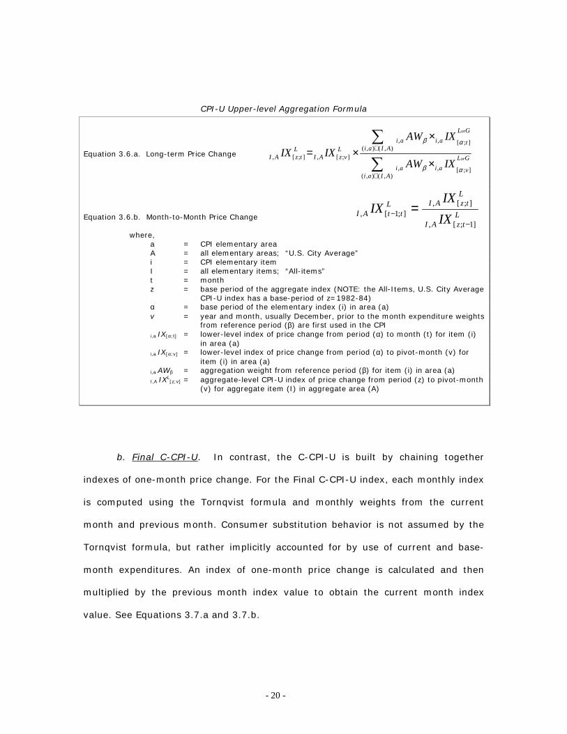
CPI-U Upper-level Aggregation Formula

Equation 3.6.a. Long-term Price Change

Equation 3.6.b. Month-to-Month Price Change

where, a = CPI elementary area A = all elementary areas; “U.S. City Average” i = CPI elementary item I = all elementary items; “All-items” t = month z = base period of the aggregate index (NOTE: the All-Items, U.S. City Average

CPI-U index has a base-period of z=1982-84) α = base period of the elementary index (i) in area (a) v = year and month, usually December, prior to the month expenditure weights

from reference period (β) are first used in the CPI i,a IX[α;t] = lower-level index of price change from period (α) to month (t) for item (i)

in area (a) i,a IX[α;v] = lower-level index of price change from period (α) to pivot-month (v) for

item (i) in area (a) i,a AWβ = aggregation weight from reference period (β) for item (i) in area (a) I,A IXL

[z;v] = aggregate-level CPI-U index of price change from period (z) to pivot-month (v) for aggregate item (I) in aggregate area (A)

b. Final C-CPI-U. In contrast, the C-CPI-U is built by chaining together

indexes of one-month price change. For the Final C-CPI-U index, each monthly index

is computed using the Tornqvist formula and monthly weights from the current

month and previous month. Consumer substitution behavior is not assumed by the

Tornqvist formula, but rather implicitly accounted for by use of current and base-

month expenditures. An index of one-month price change is calculated and then

multiplied by the previous month index value to obtain the current month index

value. See Equations 3.7.a and 3.7.b.

�

�

∈

∈

×

××=

),(),(,, ];[

),(),(,, ];[

];[,];[,

AIaiaiai

GL

v

AIaiaiai

GL

tL

vzAIL

tzAIIXAW

IXAWIXIX

or

or

β α

β α

LtzAI

LtzAIL

ttAI IXIX

IX]1;[,

];[,];1[,

−− =

- 21 -

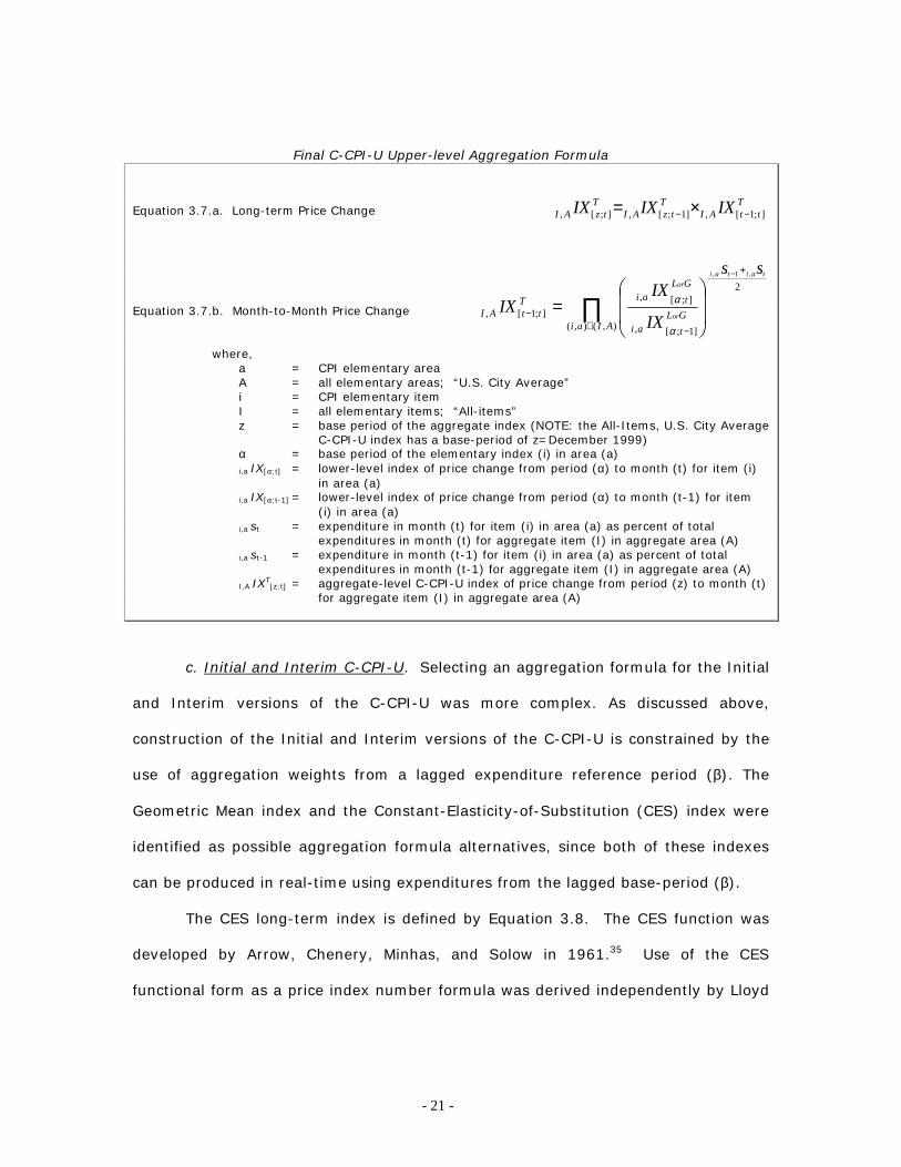
Final C-CPI-U Upper-level Aggregation Formula

Equation 3.7.a. Long-term Price Change

Equation 3.7.b. Month-to-Month Price Change

where, a = CPI elementary area A = all elementary areas; “U.S. City Average” i = CPI elementary item I = all elementary items; “All-items” z = base period of the aggregate index (NOTE: the All-Items, U.S. City Average

C-CPI-U index has a base-period of z=December 1999) α = base period of the elementary index (i) in area (a) i,a IX[α;t] = lower-level index of price change from period (α) to month (t) for item (i)

in area (a) i,a IX[α;t-1] = lower-level index of price change from period (α) to month (t-1) for item

(i) in area (a) i,a st = expenditure in month (t) for item (i) in area (a) as percent of total

expenditures in month (t) for aggregate item (I) in aggregate area (A) i,a st-1 = expenditure in month (t-1) for item (i) in area (a) as percent of total

expenditures in month (t-1) for aggregate item (I) in aggregate area (A) I,A IXT

[z;t] = aggregate-level C-CPI-U index of price change from period (z) to month (t) for aggregate item (I) in aggregate area (A)

c. Initial and Interim C-CPI-U. Selecting an aggregation formula for the Initial

and Interim versions of the C-CPI-U was more complex. As discussed above,

construction of the Initial and Interim versions of the C-CPI-U is constrained by the

use of aggregation weights from a lagged expenditure reference period (β). The

Geometric Mean index and the Constant-Elasticity-of-Substitution (CES) index were

identified as possible aggregation formula alternatives, since both of these indexes

can be produced in real-time using expenditures from the lagged base-period (β).

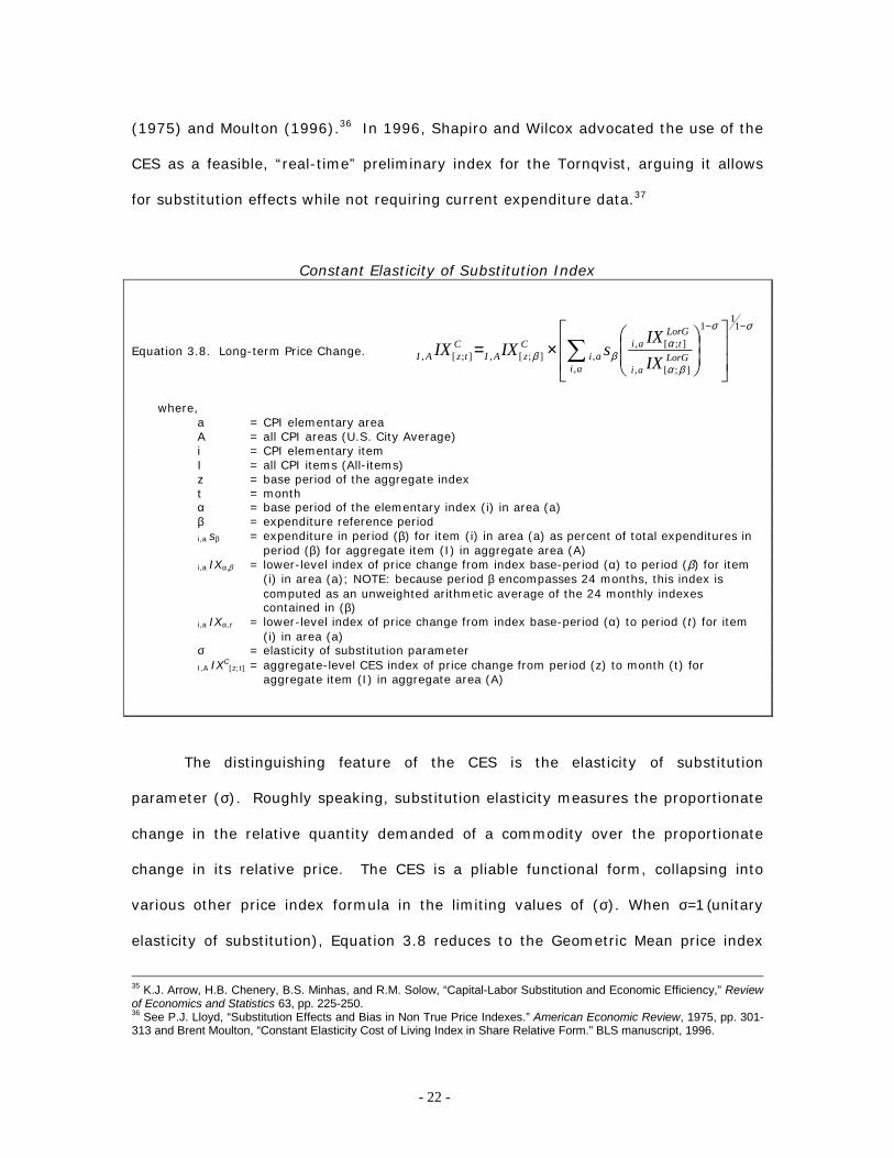
The CES long-term index is defined by Equation 3.8. The CES function was

developed by Arrow, Chenery, Minhas, and Solow in 1961.35 Use of the CES

functional form as a price index number formula was derived independently by Lloyd

TttAI

TtzAI

TtzAI IXIXIX ];1[,]1;[,];[, −− ×=

∏∈

+

−

−

−

��

�

�

��

�

�=

),(),(

2

, ]1;[

, ];[];1[,

,1,

AIai aiGLt

aiGLtT

ttAI

taitai

or

or

ss

IX

IXIX

α

α

- 22 -

(1975) and Moulton (1996).36 In 1996, Shapiro and Wilcox advocated the use of the

CES as a feasible, “real-time” preliminary index for the Tornqvist, arguing it allows

for substitution effects while not requiring current expenditure data.37

Constant Elasticity of Substitution Index

Equation 3.8. Long-term Price Change.

σσ

βα

αββ

−−

��

�

�

��

�

�

��

�

�

�×= �

11

,

1

];[,

];[,,];[,];[,

aiLorG

ai

LorGtai

aiCzAI

CtzAI IX

IXsIXIX

where, a = CPI elementary area A = all CPI areas (U.S. City Average) i = CPI elementary item I = all CPI items (All-items) z = base period of the aggregate index t = month α = base period of the elementary index (i) in area (a) β = expenditure reference period i,a sβ = expenditure in period (β) for item (i) in area (a) as percent of total expenditures in

period (β) for aggregate item (I) in aggregate area (A) i,a IXα,β = lower-level index of price change from index base-period (α) to period (β) for item

(i) in area (a); NOTE: because period β encompasses 24 months, this index is computed as an unweighted arithmetic average of the 24 monthly indexes contained in (β)

i,a IXα,τ = lower-level index of price change from index base-period (α) to period (t) for item (i) in area (a)

σ = elasticity of substitution parameter I,A IXC

[z;t] = aggregate-level CES index of price change from period (z) to month (t) for aggregate item (I) in aggregate area (A)

The distinguishing feature of the CES is the elasticity of substitution

parameter (σ). Roughly speaking, substitution elasticity measures the proportionate

change in the relative quantity demanded of a commodity over the proportionate

change in its relative price. The CES is a pliable functional form, collapsing into

various other price index formula in the limiting values of (σ). When σ=1 (unitary

elasticity of substitution), Equation 3.8 reduces to the Geometric Mean price index

35 K.J. Arrow, H.B. Chenery, B.S. Minhas, and R.M. Solow, “Capital-Labor Substitution and Economic Efficiency,” Review of Economics and Statistics 63, pp. 225-250. 36 See P.J. Lloyd, “Substitution Effects and Bias in Non True Price Indexes.” American Economic Review, 1975, pp. 301-313 and Brent Moulton, “Constant Elasticity Cost of Living Index in Share Relative Form.” BLS manuscript, 1996.

- 23 -

(Cobb-Douglas preferences). When σ=0 (zero elasticity of substitution), Equation 3.8

reduces to the Laspeyres price index (Leontief preferences).

The CES was analyzed in detail by BLS as a potential Initial and Interim C-

CPI-U aggregator. For a variety of reasons, however, the CES was judged ill-suited

as an approximation of the Final C-CPI-U. First, estimation of (σ) is problematic

from a theoretical perspective. In principle, to aggregate the 211 elementary CPI

indexes into aggregate CPI indexes the elasticity of substitution among the 211

items must be estimated in each of the 38 elementary CPI areas. This requires

estimation of a complete demand system, i.e., estimation of σ for all 22,155 possible

pairs of elementary items, in each of the 38 areas (i.e., 841,890 possible

combinations). A representative price index aggregator could have been selected

from a class of variable-elasticity-of-substitution functions to accomplish this task.38

However, a variable-elasticity aggregator suffers from several undesirable index

qualities, most notably inconsistency in aggregation, and is infeasible to produce with

the data currently available to BLS.

Alternatively, following Shapiro and Wilcox, the CES functional form with a

single value of (σ) could be assumed to hold across all possible pairs of item strata.

The CES is much more feasible to produce than a variable-elasticity aggregator. One

difficulty with using the CES, however, resides in the selection of the optimal value of

(σ). Using the laboratory of elementary price indexes and expenditure weights from

December 1986 to December 2000, monthly CES indexes were simulated in order to

find solutions to the fitting parameter, i.e., the value of (σ) yielding a CES index

best-approximating a Tornqvist index. The simulations revealed that the optimal

elasticity of substitution parameter was unstable across time (ranging from a low of

37 See, Matthew D. Shapiro and David W. Wilcox (1997): “Alternative Strategies for Aggregating Prices in the CPI,” Federal Reserve Bank of St. Louis Review, (May/June), 113-125. 38 See, for example, Nagesh S. Revankar, “A Class of Variable Elasticity of Substitution Production Functions,” Econometrica, 1971, vol. 39, issue 1, pages 61-71.

- 24 -

σ=0.06 to a high of σ=2.78). See Figure 3.4. Accordingly, the assumption of a

constant value of (σ) across month could result in specification error. This was

judged a major weakness of the CES.

Moreover, the conceptual underpinnings of the CES was judged ill-suited for

use in building a monthly-chained time series. A CES constructed with expenditure

shares derived from the same base-period month as used in the Tornqvist, i.e.

1, −tai s , could be used to approximate the Final C-CPI-U month-to-month index for

month (t). These CES month-to-month indexes could then be chained together to

produce the long-term Initial and Interim C-CPI-U index series. There are two

problems with this approach: lags in data availability preclude producing a (t-1)

weighted CES in real-time, and a monthly-chained CES could be impacted by chain

drift. Instead, expenditure shares derived from available data, i.e., βsai , , must be

used in a biennially-chained construct.

The CES functional form further requires the expenditure shares (s) to be

measured over the same time period as the denominator of the price relative.39 If

the only available expenditure shares are those derived from expenditure reference

period (β), which encompasses 24 months, it follows that the denominator price

index in the CES relative must be some average index that is representative of the

24 discrete indexes available in time (β). The choices (weighted versus unweighted

average, arithmetic versus geometric average, etc.) introduce additional estimation

complexity and potential specification error.

Due to these impediments surrounding use of the CES, the Geometric Mean

index was selected as a plausible, and simpler, approximation of the Tornqvist in

. 39 See Moulton, op. cit.

- 25 -

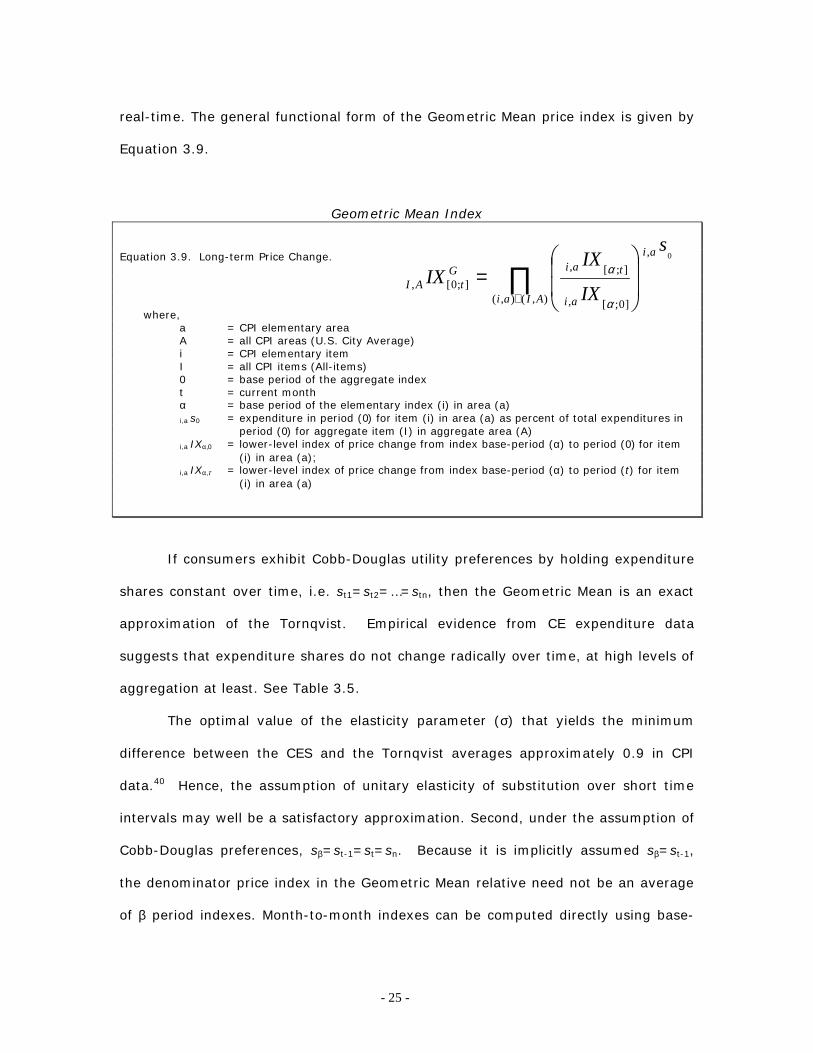
real-time. The general functional form of the Geometric Mean price index is given by

Equation 3.9.

Geometric Mean Index

Equation 3.9. Long-term Price Change.

where, a = CPI elementary area A = all CPI areas (U.S. City Average) i = CPI elementary item I = all CPI items (All-items) 0 = base period of the aggregate index t = current month α = base period of the elementary index (i) in area (a) i,a s0 = expenditure in period (0) for item (i) in area (a) as percent of total expenditures in

period (0) for aggregate item (I) in aggregate area (A) i,a IXα,0 = lower-level index of price change from index base-period (α) to period (0) for item

(i) in area (a); i,a IXα,τ = lower-level index of price change from index base-period (α) to period (t) for item

(i) in area (a)

If consumers exhibit Cobb-Douglas utility preferences by holding expenditure

shares constant over time, i.e. st1=st2=…=stn, then the Geometric Mean is an exact

approximation of the Tornqvist. Empirical evidence from CE expenditure data

suggests that expenditure shares do not change radically over time, at high levels of

aggregation at least. See Table 3.5.

The optimal value of the elasticity parameter (σ) that yields the minimum

difference between the CES and the Tornqvist averages approximately 0.9 in CPI

data.40 Hence, the assumption of unitary elasticity of substitution over short time

intervals may well be a satisfactory approximation. Second, under the assumption of

Cobb-Douglas preferences, sβ=st-1=st=sn. Because it is implicitly assumed sβ=st-1,

the denominator price index in the Geometric Mean relative need not be an average

of β period indexes. Month-to-month indexes can be computed directly using base-

∏∈

��

�

�

��

�

�=

),(),(

,

, ]0;[

, ];[];0[,

0

AIai

ai

ai

ai tGtAI

s

IX

IXIX

α

α

- 26 -

period price indexes (t-1) in the denominator, thus evading any potential

specification error caused by use of an average price relative in the denominator.

For any given month (t), the Geometric Mean month-to-month index will

differ from the corresponding Tornqvist index to the extent that the 1, −tai s differ from

tai s, and to the extent that the βsai , poorly predict 1, −tai s . Empirical evidence of

upper-level aggregation in the CPI suggests that a Geometric Mean index is biased

slightly below a Tornqvist index, when computed using expenditure shares derived

from the same base-period as the Tornqvist.41 Therefore, it is anticipated that use of

1, −tai s in a Geometric Mean index would tend to produce a lower measure of price

change than would result from use of ( 1, −tai s + tai s, )/2 in a Tornqvist index on a

consistent basis (e.g., the Geometric Mean month-to-month index averaged 0.006

percent below the corresponding Tornqvist month-to-month index in CPI data over

the 1990 to 2000 time period.) A notable exception to this general rule appears to

occur in December, where the Geometric Mean index tends to produces a higher

measure of price change than the Tornqvist. See Figure 3.5. Moreover, evidence

from CPI data further suggests that use of lagged expenditure shares βsai , in a

Geometric Mean index consistently over predicts use of 1, −tai s , albeit by a small

amount. See Figure 3.5.

In order to mitigate any specification error associated with use of a Geometric

Mean index built with lagged expenditure shares, the BLS decided to adopt an

“Adjusted Geometric Mean” approach for the Initial and Interim C-CPI-U. That is,

elementary indexes are first aggregated using the Geometric Mean index. Then, the

40 .93 from 1987 to 2000. 41 See Ana M. Aizcorbe, Robert A. Cage, and Patrick C. Jackman, “Commodity Substitution Bias in Laspeyres Indexes: Analysis Using CPI Source Data for 1982-1994,” paper presented at the Western Economic Association International Conference in San Francisco, July 1996 (Washington, DC, Bureau of Labor Statistics).

- 27 -

resulting measure of price change is multiplied by an adjustment factor (λ) that

represents the historically observed difference between Tornqvist and Geometric

Mean upper-level aggregation of CPI elementary indexes.42 See Equation 3.10.c and

3.10.d. The function of the adjustment factor is to more closely align the Geometric

Mean month-to-month index, computed with lagged base-period expenditure weights

(β), to a Tornqvist month-to-month index, computed with contemporaneous monthly

expenditures (t-1 and t).

Finally, the adjusted Geometric Mean month-to-month index is multiplied by

the previous-month C-CPI-U index value to obtain the current month C-CPI-U index

value. See Equations 3.10.a and 3.10.b. Note that each Interim month-to-month

index is chained onto an Interim long-term index value, with the exception of the

January index which is chained onto the previous year December index, which is in

Final C-CPI-U form. Each Initial month-to-month index is chained onto an Initial

long-term index value, with the exception of the January index which is chained onto

the previous year December index, which is in Interim C-CPI-U form.

For all months of 2002 and 2003, the adjustment factor has been set equal to

unity. BLS plans to use Initial and Interim indexes calculated for 2002 and 2003, in

conjunction with Initial and Interim versions of 2000 and 2001, to evaluate further

how the Geometric Mean behaves relative to the Tornqvist. A permanent

methodology for calculating the adjustment factor will be implemented at a future

date.

42 The set of data available to compute the adjustment factor is limited to all time periods for which the Final C-CPI-U has been computed. In 2002, for example, Final C-CPI-U indexes area available only for the 12 months of 2000. In 2003, an additional 12 months of data will become available. Lacking a sufficient time-series of historical data, the adjustment factor for 2002 and 2003 Initial and Interim C-CPI-U indexes will be set equal to λ=1. Official methodology for calculating the adjustment factor will be implemented with the calculation of January 2004 Initial indexes, when 36 months of historical data will be available.

- 28 -

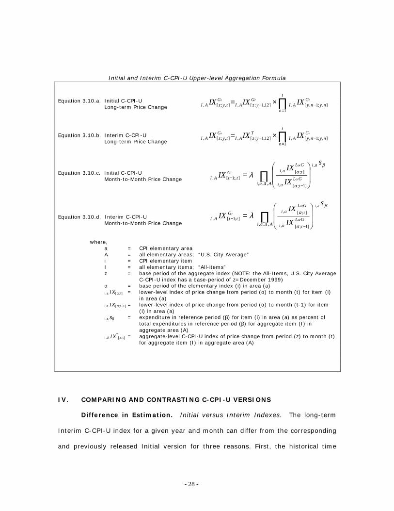
Initial and Interim C-CPI-U Upper-level Aggregation Formula

Equation 3.10.a. Initial C-CPI-U Long-term Price Change

Equation 3.10.b. Interim C-CPI-U

Long-term Price Change

Equation 3.10.c. Initial C-CPI-U Month-to-Month Price Change Equation 3.10.d. Interim C-CPI-U

Month-to-Month Price Change where, a = CPI elementary area A = all elementary areas; “U.S. City Average” i = CPI elementary item I = all elementary items; “All-items” z = base period of the aggregate index (NOTE: the All-Items, U.S. City Average

C-CPI-U index has a base-period of z=December 1999) α = base period of the elementary index (i) in area (a) i,a IX[α;t] = lower-level index of price change from period (α) to month (t) for item (i)

in area (a) i,a IX[α;t-1] = lower-level index of price change from period (α) to month (t-1) for item

(i) in area (a) i,a sβ = expenditure in reference period (β) for item (i) in area (a) as percent of

total expenditures in reference period (β) for aggregate item (I) in aggregate area (A)

I,A IXT[z;t] = aggregate-level C-CPI-U index of price change from period (z) to month (t)

for aggregate item (I) in aggregate area (A)

IV. COMPARING AND CONTRASTING C-CPI-U VERSIONS

Difference in Estimation. Initial versus Interim Indexes. The long-term

Interim C-CPI-U index for a given year and month can differ from the corresponding

and previously released Initial version for three reasons. First, the historical time

∏=

−− ×=t

n

GnynyAI

GyzAI

GtyzAI

iri IXIXIX1

],;1,[,]12,1;[,],;[,

∏=

−− ×=t

n

GnynyAI

TyzAI

GtyzAI

rr IXIXIX1

],;1,[,]12,1;[,],;[,

∏∈ −

− ��

�

�

��

�

�=

AIai

ai

aiGLt

aiGLtG

ttAI

s

IX

IXIX

or

or

i

,,

,

, ]1;[

, ];[];,1[,

β

α

αλ

∏∈ −

− ��

�

�

��

�

�=

AIai aiGLt

aiGLtG

ttAI

s

IX

IXIX

ai

or

or

r

,, , ]1;[

, ];[];1[,

, β

α

αλ

- 29 -

series to which the Interim index is chained will contain an additional year of Final C-

CPI-U indexes. Consequently, the terminal December index value to which the

January Interim index is chained may be different from the terminal December index

to which the Initial index is chained. Second, the relative expenditure weight

patterns used for aggregation may be different. This is highly probable in odd-

numbered years – when the expenditure reference period (β) used for the calculation

of Initial and Interim indexes will be different. For example, 2003 Initial indexes will

use β=1999,2000, but 2003 Interim indexes (released in 2004) will use

β=2001,2002. The aggregation weights for even-year Initial and Interim indexes will

be identical. Third, the adjustment factor (λ) applied to the Initial Geometric Mean

aggregation and the Interim Geometric Mean aggregation may be different.

Final versus Interim Indexes. Similarly, the long-term Final C-CPI-U index for

a given year and month can differ from the corresponding and previously released

Initial and Interim versions for three reasons. First, the historical time series to

which the Final index is chained will contain additional years of Final C-CPI-U

indexes. Consequently, the terminal December index value to which the January

Final index is chained may be different from the terminal December indexes to which

the Initial and Interim indexes were chained. Second, the relative expenditure weight

patterns used for aggregation most likely will be different. The difference in

aggregation weights is the primary distinction in functional form between the Final

and two preliminary versions of the C-CPI-U. Variation in the relative monthly

expenditures used for the Final from the lagged constant-within-year relative

expenditures used for the Initial and Interim may result in differing estimates of

aggregate price change. Third, off-cycle elementary index values may be slightly

different between the Final and preliminary versions, as the Final version will use

geometric averaging of bounding month indexes.

- 30 -

V. COMPARING AND CONTRASTING THE C-CPI-U AND THE CPI-U

Difference in Estimation. Because the CPI-U and all three versions of the

C-CPI-U differ in the set of input elementary price indexes and expenditures used for

aggregation, as well as in aggregation formula, each index may yield a different

measure of aggregate price change for a given year and month. Table 5.1

summarizes the differences between CPI-U and C-CPI-U index construction.

The Initial C-CPI-U index is published in the same news release as the CPI-U.

The long-term index values are not directly comparable, as the CPI-U will be on a

1982-84=100 base and the C-CPI-U will be on a December 1999=100 base. The

Initial C-CPI-U month-to-month index for a given year and month will differ from the

corresponding CPI-U index by upper-level aggregation method only. The input prices

and expenditures will be the same. Similarly, the Interim C-CPI-U month-to-month

indexes will differ from the CPI-U month-to-month indexes in aggregation method.

In addition, odd-year Interim indexes will differ in input expenditures used for

aggregation. Final C-CPI-U month-to-month indexes will differ from the CPI-U

month-to-month indexes in all aspects of index construction: (a) the input

elementary price indexes will be the same, with the exception of off-cycle bimonthly

indexes; (b) input elementary expenditures will be different, and (c) aggregation

method will differ.

Index Simulations. Simulating official estimation methodology, a biennially

weight-updated CPI-U index series was calculated and compared to a Final C-CPI-U

index series over the 1990 to 2000 period in order to measure the anticipated

difference between the two series. See Figure 5.1. The average difference between

the weight-updated CPI-U and the C-CPI-U was 0.32 percent per year over this time

period. See Table 5.2. This estimate is at the upper end of the 0.1 percent to 0.4

percent range of upper-level substitution bias estimated in prior BLS research, in

- 31 -

which the average annual percent difference was closer to 0.2 percent. Simulations

for the 1990 to 2000 period define the range at 0.1 percent to 0.5 percent.

There are several factors contributing to this result. First, the prior average of

0.2 percent was based on data from 1991 to 1995 using the 1987 CPI market basket

structure of 207 elementary items and 46 elementary areas (i.e., 9,522 elementary

cells). The estimated average in Table 5.2 of 0.3 percent is based on the 1998 CPI

market basket structure of 8,018 elementary cells from 1990 to 2000. In order to

obtain data on the 1998 structure for years prior to 1998, price indexes and

expenditures were approximated using a rough concordance between the old and

new structures. Moreover, the current estimate is based on composite-estimated-

and-raked biennial expenditures whereas the prior estimates were not. These

differences function to produce an average annual substitution effect estimate for the

overlap years of 1991 to 1995 that differs by 0.05 percent, i.e. 0.24 percent versus

0.19 percent.

Second, the gap between the weight-updated CPI-U and C-CPI-U appears to

have widened in the later part of the decade. The average annual percent difference

between the two indexes rose to 0.40 percent in 1996 to 2000, almost double that

observed from 1991-1995. Analogously, the percent difference in simulated weight-

updated CPI-U and C-CPI-U 12-month indexes steadily increased over the decade.

See Figure 5.2.

A likely contributor to the growing gap is increased dispersion in relative

elementary index changes. In general, the CPI-U and the C-CPI-U will diverge to the

extent that (a) component elementary indexes have rates of inflation that differ from

each other, and (b) expenditure shares reflect a shift in consumer purchases toward

those item categories that have fallen in relative price. Consequently, when there is

- 32 -

more variation in price movement among elementary indexes, there is more room

for the Laspeyres-based CPI-U and the superlative-based C-CPI-U to diverge.

Price change in CPI elementary indexes varied more widely during the later

part of the 1990s. See Figure 5.3. Two examples of indexes with unusual index

movements in 1999 and 2000 are computers and natural gas. The series for

ITEM=EE01 “Personal computers and peripheral equipment” decreased by 22.7

percent from December 1999 to December 2000. In contrast, the series for

ITEM=HF02 “Utility natural gas service” increased by 36.7 percent over the same

interval. The median elementary index change over this time period was 2.2

percent.

The significance of outlier elementary index series can by quantified by

excluding them from CPI-U and C-CPI-U calculations and measuring the gap between

the resulting “trimmed” indexes. This exercise was performed using the December

1999 to December 2000 12-month simulated index for the C-CPI-U and weight-

updated CPI-U, at varying outlier thresholds. See Table 5.3. When computing the

indexes using the set of elementary indexes in the middle quartile, i.e. trimming the

lower and upper quartiles from the calculations, the percent difference between the

CPI-U and C-CPI-U is diminutive, 0.07 percent. The gap increases to 0.2 percent

when the set of elementary items used in the calculations is limited to those that

increased or decreased in price by 10 percent or less (roughly 75 percent of all

elementary items over the December 1999 to December 2000 period). When the set

is expanded to include all items exhibiting 20 percent price change (90 percent of all

elementary items) the gap increases to 0.3 percent. The difference between the

CPI-U and C-CPI-U is greatest when restricting aggregation over the lowest quartile

of elementary index price change (1.5 percent) and highest quartile (0.7 percent).

These trimmed indexes demonstrate that extreme changes in elementary price

- 33 -

indexes cause the CPI-U and C-CPI-U to diverge, and suggest that deflationary

outliers contribute heavily to the gap.

VI. INAUGURAL PUBLISHED INDEXES C-CPI-U indexes were published for the first time in August 2002. Indexes are

published for the urban population only. There are no plans at this time to calculate

and publish a C-CPI-W. Published C-CPI-U indexes are available for the U.S. City

Average only. No regional or local area indexes are published. Moreover, a limited

set of indexes are available. See Table 6.1.

Table 6.2, and Figure 6.1, display the inaugural published values of the

C-CPI-U in relation to the CPI-U.43 The most surprising result was the 0.8

percentage point gap between the two estimates of 12-month change during

calendar year 2000, which was the only year for which the C-CPI-U index values

were published in Final form. The reasons for this were discussed in section V

above; additionally, rounding played a role in exaggerating the differences. The

Interim and Initial values for 2001 and 2002 indicated some significant narrowing of

the gap in those years.

VII. 2003 REVISIONS AND MOST CURRENT PUBLISHED INDEXES

In accordance with its previously-announced schedule, the BLS issued the

first set of revised values of the C-CPI-U effective with the release of January 2003

CPI data. While the magnitude of these revisions is expected to be small in the

aggregate, in theory each monthly index is subject to two revisions until monthly

expenditure data have been generated for that period and introduced two years

later. With the availability of consumer expenditure data for 2001, the monthly

C-CPI-U index values for 2001 became Final, and the values for 2002 moved from

43 It should be noted that the published values for 2000 differ from the simulated values reported in section V for a variety of minor reasons. For example, the CPI-U values in Table 5.2 were simulated using a biennial weight update process,

- 34 -

Initial to Interim status. The revised index values and 12-month changes are shown

in Table 7.1.

In most cases, the revisions were upward and had the effect of narrowing the

differences between the C-CPI-U and the CPI-U index series. At the All Items level,

the Final C-CPI-U index for December 2001 increased from 103.6 to 103.9 and the

12-month change rose from 1.0 to 1.3 percent, compared to a 1.6 percent increase

in the CPI-U. It should be noted that rounding exaggerates the impact of revisions

in this case: the unrounded change in the December 2001 index level is only 0.22

(103.65 to 103.87).

The bulk of the 2001 revisions can be attributed to a small number of item

categories. The three largest contributors—owner’s equivalent rent, natural gas, and

gasoline—account for about 92 percent of the revision to the All Items C-CPI-U for

the period December 2000 to December 2001. In each case the item’s expenditure

share moved in the same direction as its relative price change, indicating less than

unitary elasticity of substitution. Owners’ equivalent rent rose somewhat more than

the average CPI during 2001. Its overall impact results from its very large weight.

Natural gas and gasoline prices both rose sharply early in 2001, then fell sharply.

Their impacts result from their extreme price movements.

C-CPI-U index levels for 2002 change only because they are spliced onto the

revised 2001 Final values. Rates of change in months after December 2001 are

unaffected by the revisions, except for rounding. Percent index changes during 2002

and 2003 are still based on the geometric mean formula and weights from 1999-

2000, as they were before the revisions. At the All Items level, the CPI-U increased

2.4 percent from December 2001 to December 2002 and the C-CPI-U increased 2.1

percent.

whereas the published CPI-U in that year used 1993-95 base period weights. The values in Table 5.2 also are annual-

- 35 -

Comparisons with Personal Consumption Expenditure Index. In 1996,

the Bureau of Economic Analysis (BEA) at the Department of Commerce introduced

chain-type, annual-weighted indexes as its featured measures of real output and

prices of the National Income and Product Accounts (NIPA’s). The chain-type price

index for personal consumption expenditures (PCE) is similar in concept to the

C-CPI-U in several aspects. Both employ a superlative aggregator—BEA’s PCE price

index is constructed using the Fisher Ideal index formula. Both are chained, albeit

the C-CPI-U at monthly intervals with monthly weights, while the PCE index is

chained quarterly, with annual adjustments. On the other hand, there are significant

distinctions between the two series. Notably, the PCE index is broader in scope and

includes spending on behalf of consumers by employers and government health

agencies. The PCE index also uses NIPA weights rather than Consumer Expenditure

Survey values, and relies in part on price series other than those used in the CPI.

Table 7.2 compares December-to-December changes in the CPI-U, the

C-CPI-U, and the PCE index for the three years for which the C-CPI-U has been

published. As the table shows, the C-CPI-U and PCE series are remarkably close

given the differences in their scope and construction. This lends some indirect

support to the C-CPI-U. Note that the 2002 C-CPI-U estimate is not a Final number.

VIII. SUMMARY AND DIRECTIONS OF FURTHER RESEARCH

The release of the C-CPI-U marks a significant step forward in the U.S. CPI

program. A superlative index formula, by employing expenditure data from two

separate points in time rather than from a single base period, is designed to reflect

substitution among items in response to changes in relative prices and to provide a

closer approximation to a cost-of-living index than is possible using the Laspeyres

average figures, rather than December-to-December changes.

- 36 -

formula. The unavoidable delays in receiving expenditure data result in the inability

to produce the final C-CPI-U on the same schedule as the fixed-base CPI-U and

CPI-W indexes. The BLS therefore designed the C-CPI-U as its first CPI series to be

produced in preliminary form and subject to revision. In August 2002 the inaugural

C-CPI-U series were released, followed in February 2003 by the first set of annual

revisions.

One notable difference between the C-CPI-U and the existing fixed-base

indexes is the interpretation of the sub-indexes--e.g. food, energy, all items less

food and energy, etc. In the fixed-base CPIs, the subindexes are separable and

additive. In the C-CPI-U the subindexes are conditional upon the behavior of the

expenditures and prices of items not included within the subindex, and are therefore

not additive. For example, in the C-CPI-U, the behavior of the food index is a

function not only of the expenditure and price movements of the food items included

within the food aggregate, but also of the expenditure and price movements of all

other components within the All Items C-CPI-U. In addition, the All Items C-CPI-U in

general is not the weighted average of the subindexes that comprise it, either for all

211 item strata or for sub-aggregates such as food, energy, and all items less food

and energy. That is, the C-CPI-U is not consistent in aggregation.

As discussed above in section III, many challenges faced the BLS in the

course of designing the C-CPI-U. Corresponding to each of these challenges are

issues that can be addressed in the future with the aid of growing time series of

published data. Further analysis may, in some cases, lead to modifications in the

way the C-CPI-U is constructed. Among the issues that the BLS is planning to study

are:

(i) Analyze the gap between the CPI-U and the C-CPI-U. Sections V and VI

described how the difference between the two estimates of annual inflation widened

- 37 -

in the late 1990s. In the first year of published C-CPI-U data, the gap of 0.8

percentage point greatly exceeded the earlier BLS prediction range. The gap was

smaller in 2001 than in 2002, and it is reasonable to expect that during the next few

years CPI-U inflation estimates will exceed those of the C-CPI-U by more than 0.2

percentage point but less than 0.8 percentage point. BLS staff are now working to

develop alternative means of decomposing the inflation differences, in order to more

easily identify the contributions of individual index series.44

(ii) Determine the best estimator for the Initial and Interim indexes. The

BLS has no experience yet in the C-CPI-U upon which to base estimates of the future

size of revisions between Initial and Final index values. The revisions to 2001

Interim indexes were not unduly large, but the fact that they were upward revisions

was relatively unusual compared to most years in historical simulations. Thus far,

the simulation studies have been insufficient to estimate an adjustment factor

reliably, and thus far the BLS has employed a factor of one—i.e., using an

unadjusted geometric mean formula—to produce the preliminary index values.

Future work will address how best to estimate the adjustment factor when longer

time series are available for that purpose. Other potential topics include the use of

different factors for different months of the year and, more generally, the analysis of

alternative formulas and approaches to predicting the final superlative values.

(iii) Evaluate the monthly weights. The issues of seasonality, volatility,

sampling error, and other special features of the Consumer Expenditure Survey data

comprise a rich and important area of research. The BLS plans to study how best to

44 On the topic of superlative index decomposition, see Marshall B. Reinsdorf, W. Erwin Diewert and Christian Ehemann, “Additive decompositions for Fisher, Tornqvist and geometric mean indexes,” Journal of Economic and Social Measurement 28, pps.51–61. .

- 38 -

deal with seasonal and durable goods, and whether alternative methods of composite

weight estimation could improve index performance.

(iv) Evaluate the elementary price indexes. Parallel to the analysis of weight

data, research on elementary price indexes would include outlier mitigation,

collapsing of areas, composite estimation, and other means of reducing volatility and

making the price series more appropriate to their use in a monthly superlative

formula.

In the future, with the production and publication of a longer time series, the

BLS also will revisit the issue of generating seasonally adjusted C-CPI-U indexes. It

should be noted that the method employed in the CPI-U, dependent seasonal

adjustment (i.e., aggregating a selected set of seasonally adjusted components to

obtain seasonally adjusted aggregates), is inappropriate for the C-CPI-U, since it is

not consistent in aggregation. The Bureau also intends to produce and publish

statistical measures of reliability for the C-CPI-U such as are presently published for

the fixed-base CPIs.

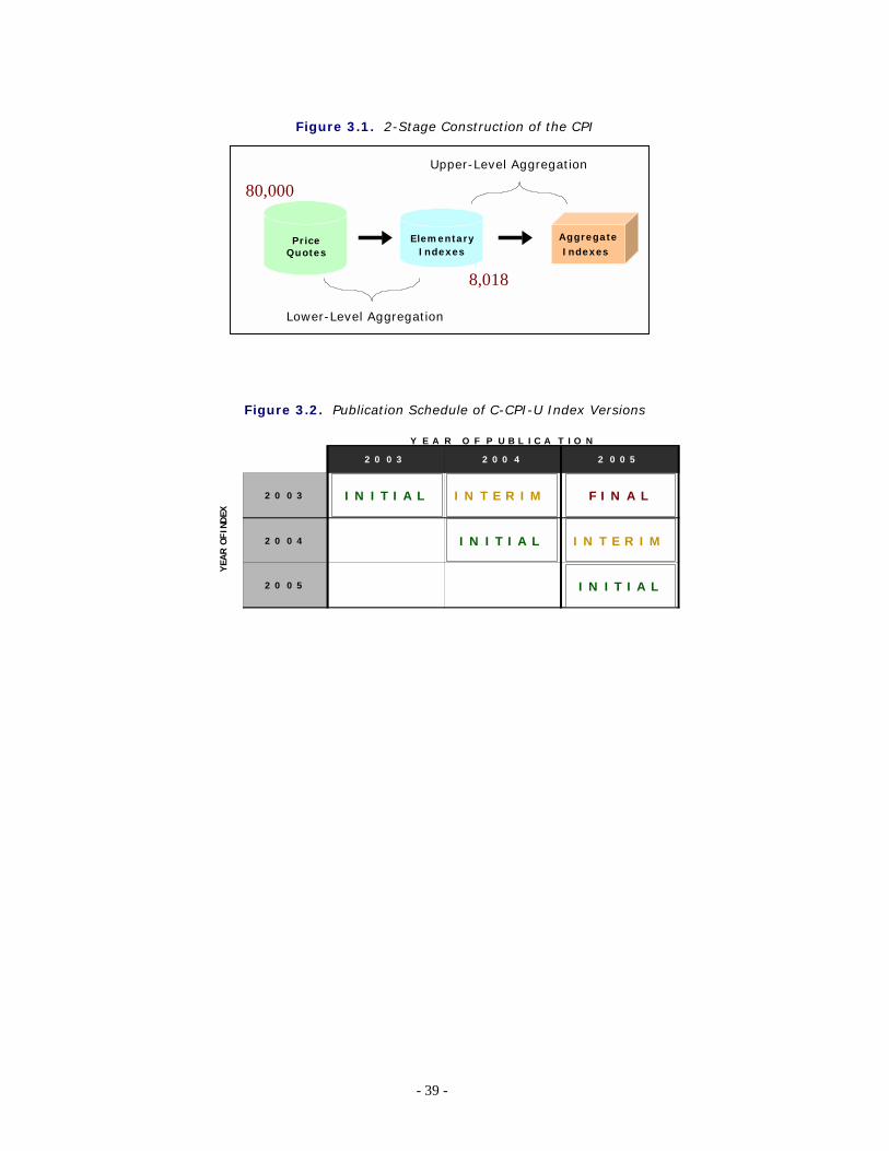
- 39 -

Figure 3.1. 2-Stage Construction of the CPI

Figure 3.2. Publication Schedule of C-CPI-U Index Versions

AggregateIndexes

Lower-Level AggregationLower-Level Aggregation

Upper-Level AggregationUpper-Level Aggregation

PriceQuotes

80,000

ElementaryIndexes

8,018

2 0 0 3 2 0 0 4 2 0 0 5

2 0 0 3

2 0 0 4

2 0 0 5

Y E A R O F P U B L I C A T I O N

YEA

R O

F IN

DEX

I N I T I A L

I N I T I A L

I N T E R I M F I N A L

I N T E R I M

I N I T I A L

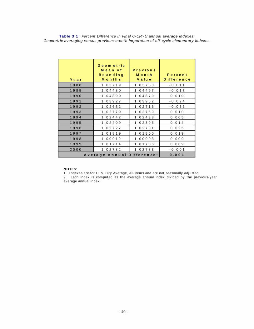
- 40 -

Table 3.1. Percent Difference in Final C-CPI-U annual average indexes: Geometric averaging versus previous-month imputation of off-cycle elementary indexes.

NOTES: 1. Indexes are for U. S. City Average, All-items and are not seasonally adjusted. 2. Each index is computed as the average annual index divided by the previous-year average annual index.

Y e a r

G e o m e t r ic M e a n o f

B o u n d in g M o n t h s

P r e v io u s M o n t h V a lu e

P e r c e n t D if fe r e n c e

1 9 8 8 1 .0 3 7 1 9 1 .0 3 7 3 0 -0 .0 1 1

1 9 8 9 1 .0 4 4 8 0 1 .0 4 4 9 7 -0 .0 1 7

1 9 9 0 1 .0 4 8 9 0 1 .0 4 8 7 9 0 .0 1 0

1 9 9 1 1 .0 3 9 2 7 1 .0 3 9 5 2 -0 .0 2 4

1 9 9 2 1 .0 2 6 8 2 1 .0 2 7 1 6 -0 .0 3 3

1 9 9 3 1 .0 2 7 7 9 1 .0 2 7 6 9 0 .0 1 0

1 9 9 4 1 .0 2 4 4 2 1 .0 2 4 3 8 0 .0 0 5

1 9 9 5 1 .0 2 4 0 9 1 .0 2 3 9 5 0 .0 1 4

1 9 9 6 1 .0 2 7 2 7 1 .0 2 7 0 1 0 .0 2 5

1 9 9 7 1 .0 1 8 1 9 1 .0 1 8 0 0 0 .0 1 9

1 9 9 8 1 .0 0 9 1 2 1 .0 0 9 0 3 0 .0 0 9

1 9 9 9 1 .0 1 7 1 4 1 .0 1 7 0 5 0 .0 0 9

2 0 0 0 1 .0 2 7 8 2 1 .0 2 7 8 3 -0 .0 0 1

A v e r a g e A n n u a l D if f e r e n c e : 0 .0 0 1

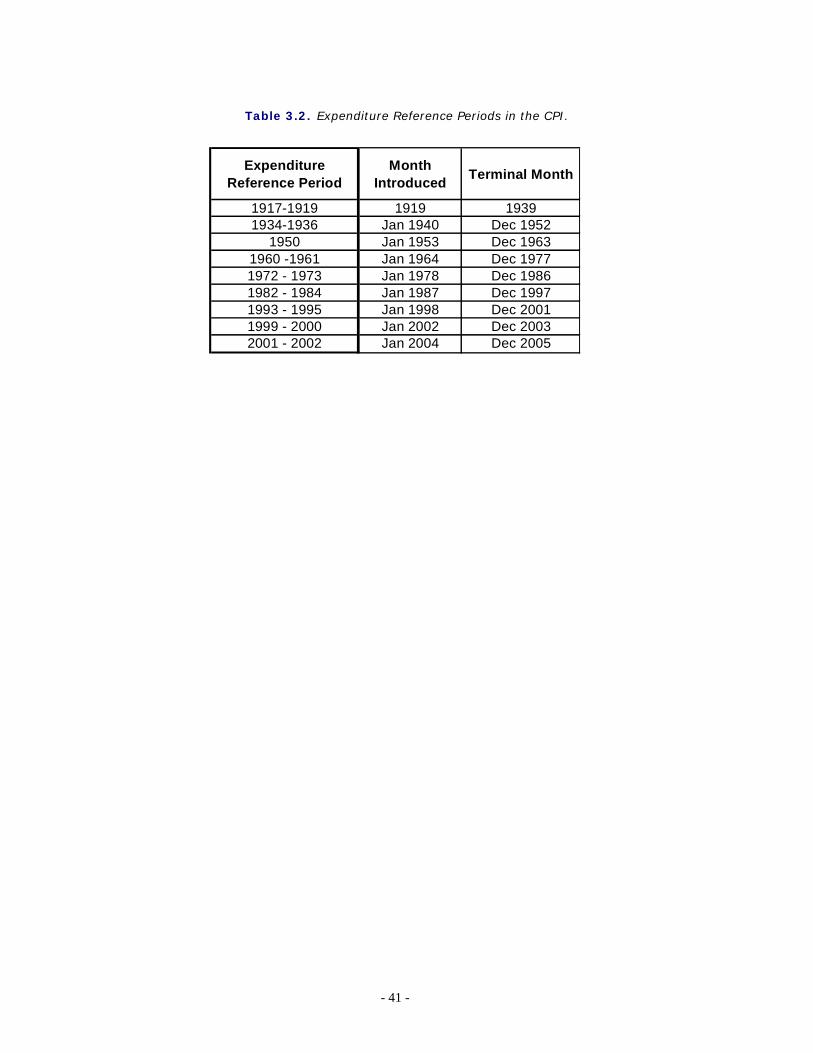
- 41 -

Table 3.2. Expenditure Reference Periods in the CPI.

Expenditure Reference Period

Month Introduced Terminal Month

1917-1919 1919 19391934-1936 Jan 1940 Dec 1952

1950 Jan 1953 Dec 19631960 -1961 Jan 1964 Dec 19771972 - 1973 Jan 1978 Dec 19861982 - 1984 Jan 1987 Dec 19971993 - 1995 Jan 1998 Dec 20011999 - 2000 Jan 2002 Dec 20032001 - 2002 Jan 2004 Dec 2005

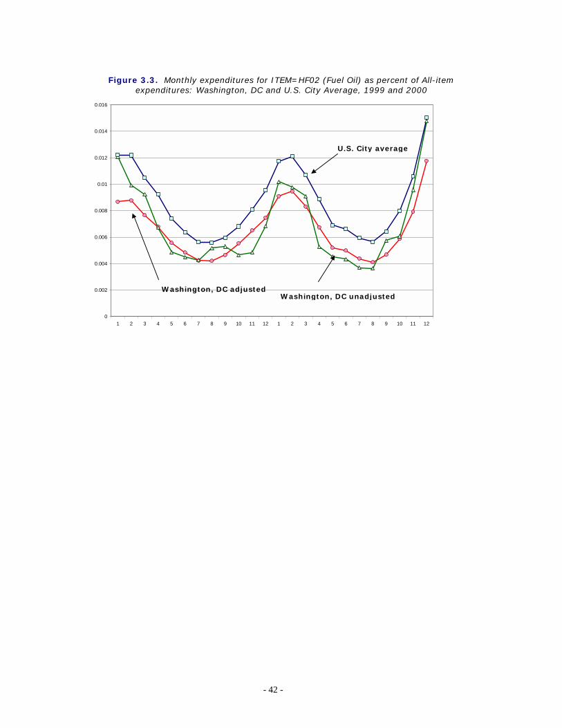
- 42 -

0

0.002

0.004

0.006

0.008

0.01

0.012

0.014

0.016

1 2 3 4 5 6 7 8 9 10 11 12 1 2 3 4 5 6 7 8 9 10 11 12

Figure 3.3. Monthly expenditures for ITEM=HF02 (Fuel Oil) as percent of All-item expenditures: Washington, DC and U.S. City Average, 1999 and 2000

U.S. City average

Washington, DC adjusted Washington, DC unadjusted

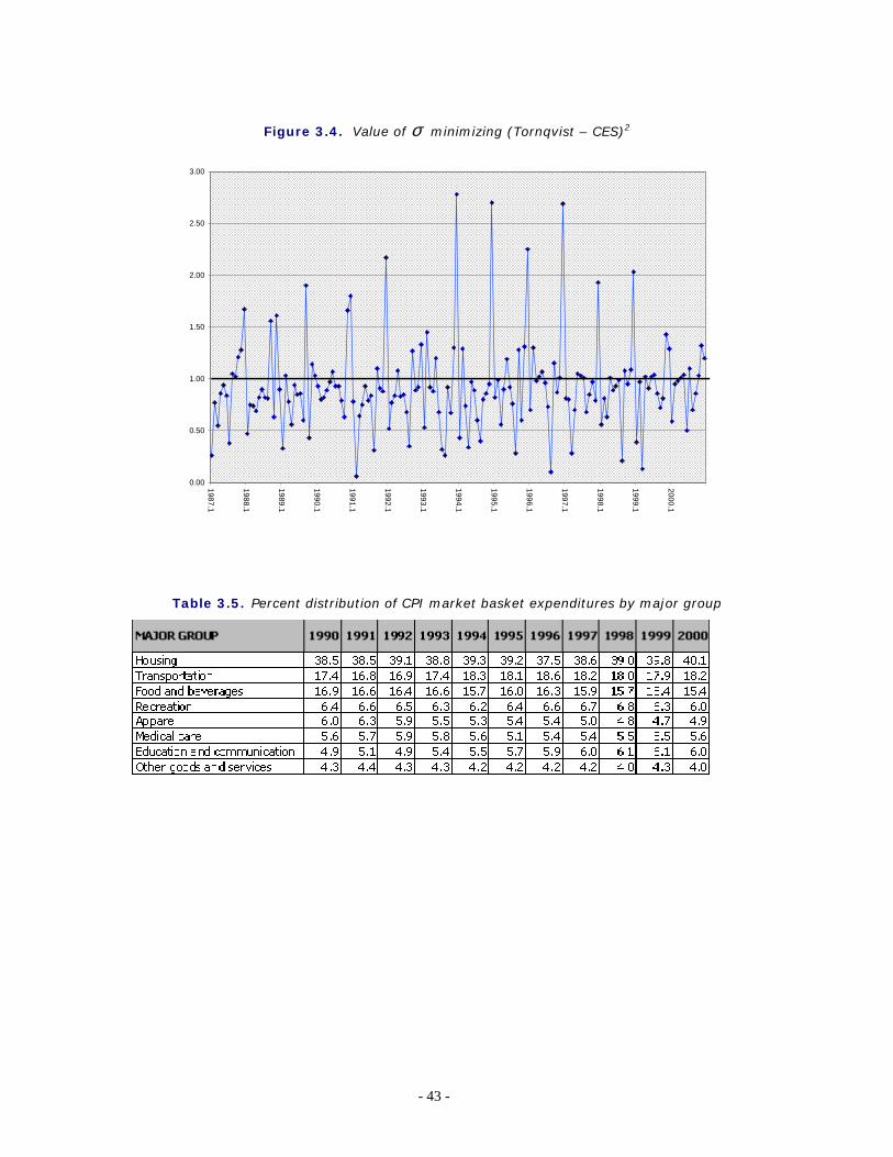
- 43 -

Figure 3.4. Value of σ minimizing (Tornqvist – CES)2

Table 3.5. Percent distribution of CPI market basket expenditures by major group

0.00

0.50

1.00

1.50

2.00

2.50

3.00

1987.1

1988.1

1989.1

1990.1

1991.1

1992.1

1993.1

1994.1

1995.1

1996.1

1997.1

1998.1

1999.1

2000.1

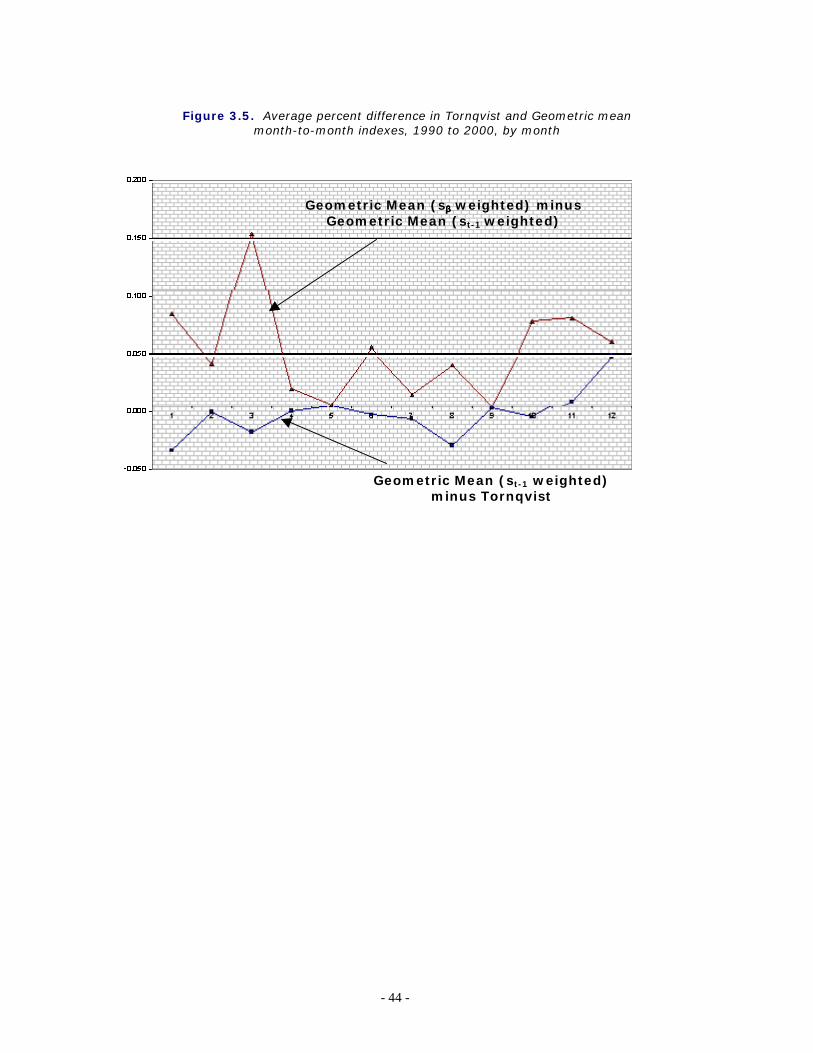
- 44 -

Figure 3.5. Average percent difference in Tornqvist and Geometric mean month-to-month indexes, 1990 to 2000, by month

Geometric Mean (st-1 weighted) minus Tornqvist

Geometric Mean (sββββ weighted) minus Geometric Mean (st-1 weighted)

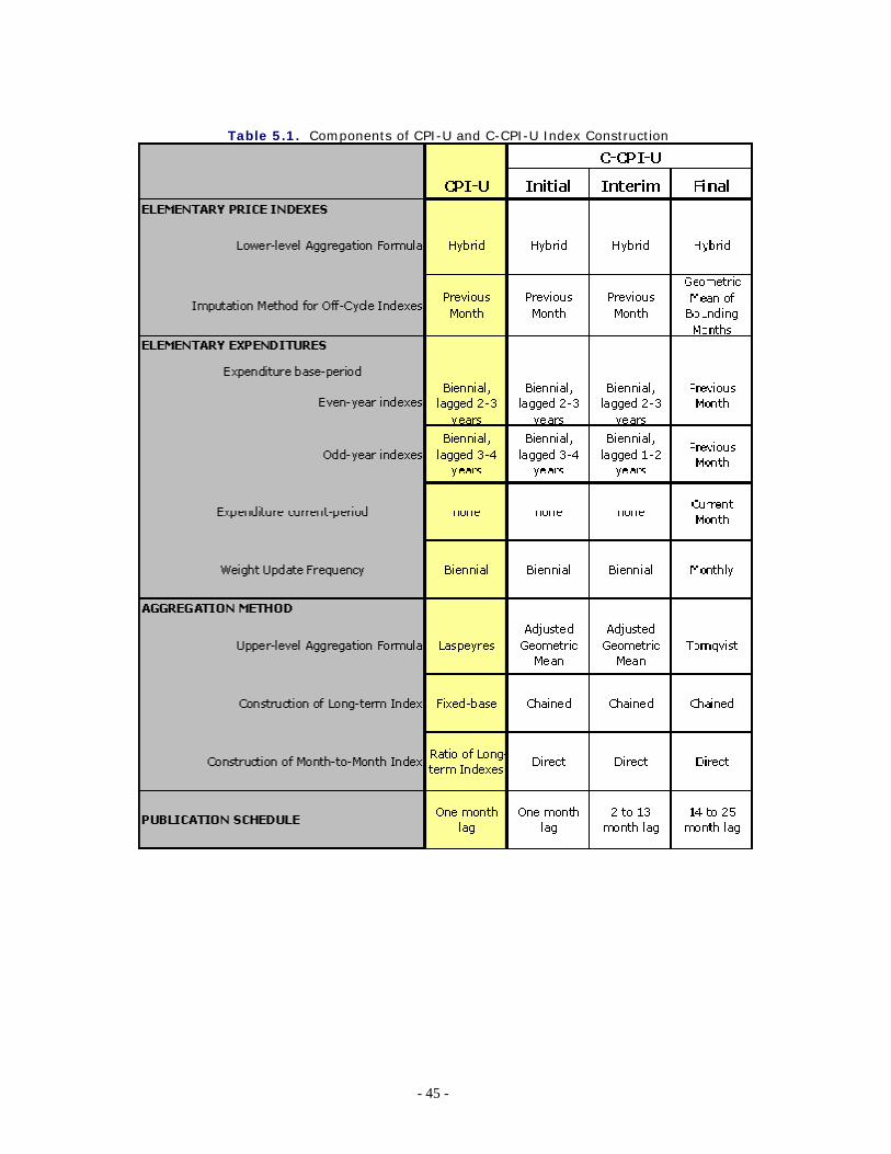
- 45 -

Table 5.1. Components of CPI-U and C-CPI-U Index Construction

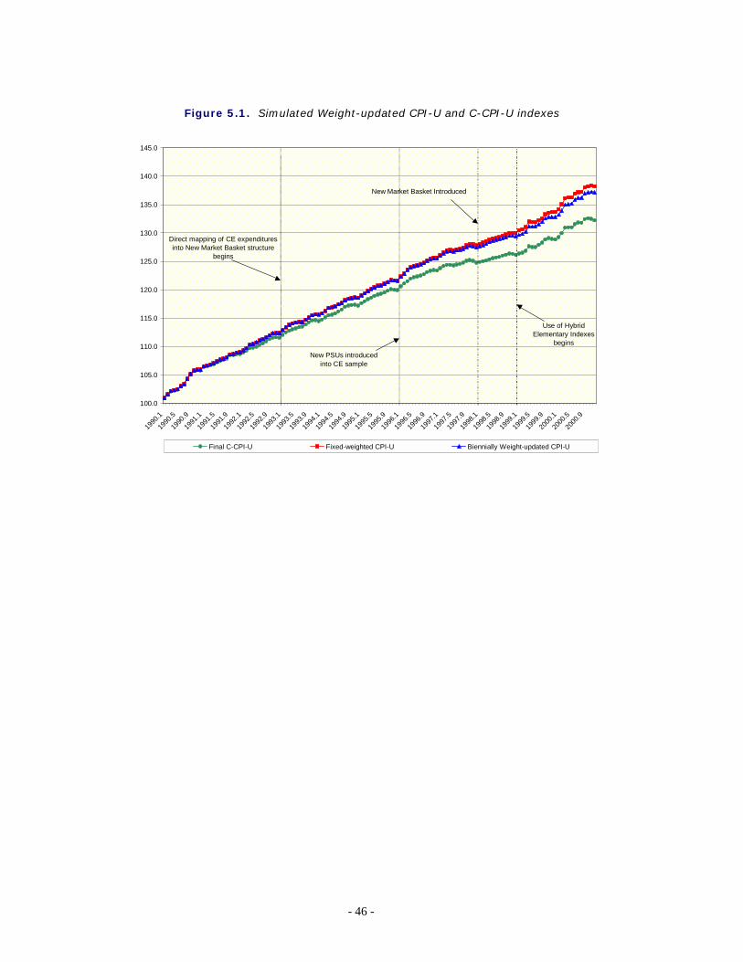
- 46 -

Figure 5.1. Simulated Weight-updated CPI-U and C-CPI-U indexes

100.0

105.0

110.0

115.0

120.0

125.0

130.0

135.0

140.0

145.0

1990

.1

1990

.5

1990

.9

1991

.1

1991

.5

1991

.9

1992

.1

1992

.5

1992

.9

1993

.1

1993

.5

1993

.9

1994

.1

1994

.5

1994

.9

1995

.1

1995

.5

1995

.9

1996

.1

1996

.5

1996

.9

1997

.1

1997

.5

1997

.9

1998

.1

1998

.5

1998

.9

1999

.1

1999

.5

1999

.9

2000

.1

2000

.5

2000

.9

Final C-CPI-U Fixed-weighted CPI-U Biennially Weight-updated CPI-U

New Market Basket Introduced

Use of HybridElementary Indexes

begins

New PSUs introducedinto CE sample

Direct mapping of CE expendituresinto New Market Basket structure

begins

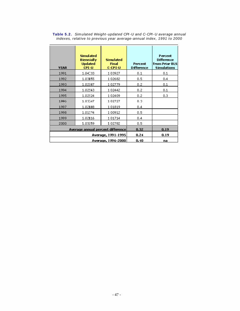
- 47 -

Table 5.2. Simulated Weight-updated CPI-U and C-CPI-U average annual indexes, relative to previous year average-annual index, 1991 to 2000

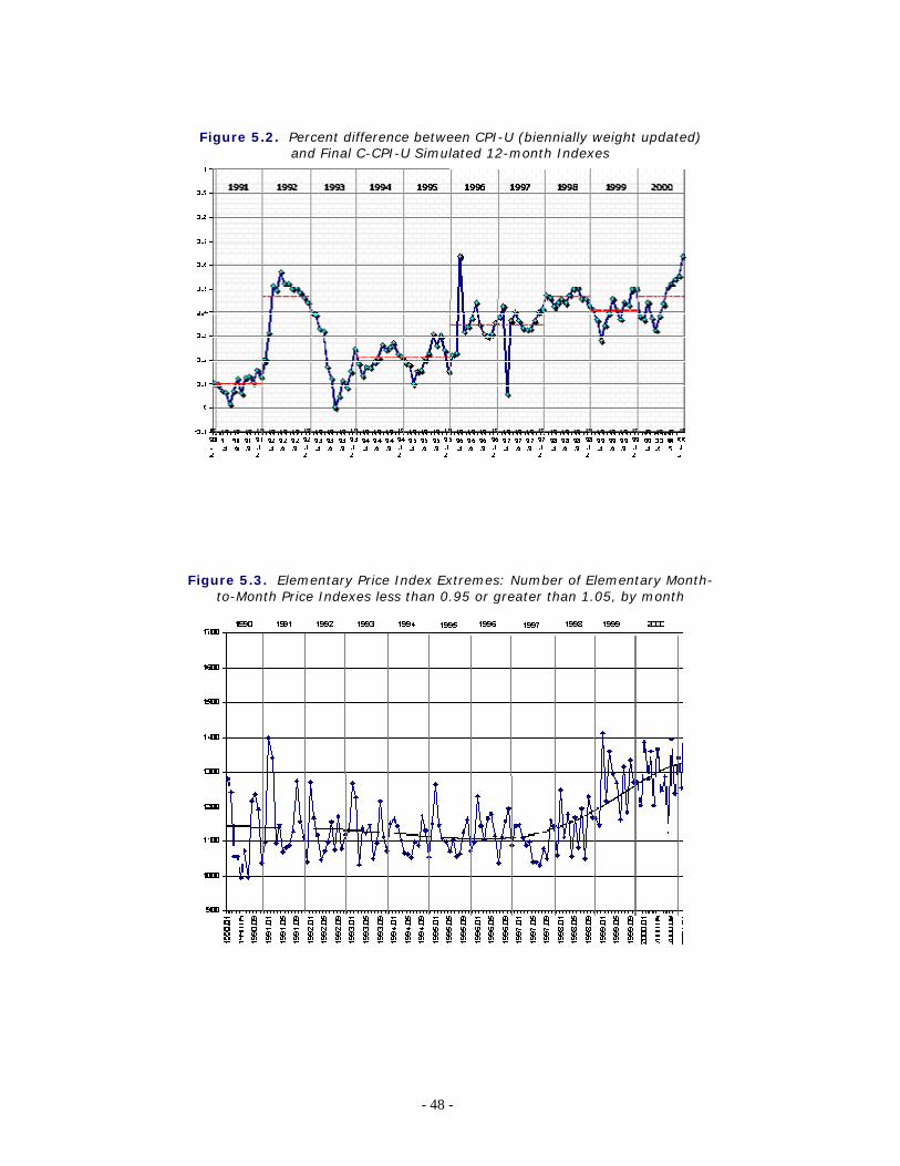
- 48 -

Figure 5.2. Percent difference between CPI-U (biennially weight updated) and Final C-CPI-U Simulated 12-month Indexes

Figure 5.3. Elementary Price Index Extremes: Number of Elementary Month-to-Month Price Indexes less than 0.95 or greater than 1.05, by month

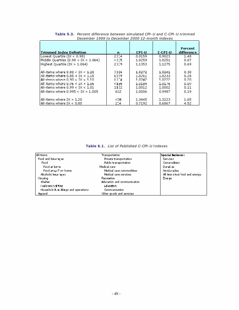
- 49 -

Table 5.3. Percent difference between simulated CPI-U and C-CPI-U trimmed December 1999 to December 2000 12-month indexes

Table 6.1. List of Published C-CPI-U Indexes

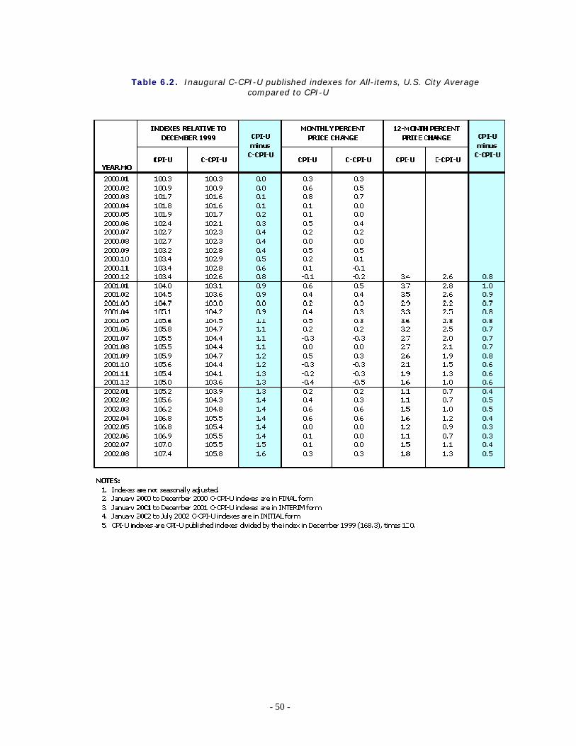
- 50 -

Table 6.2. Inaugural C-CPI-U published indexes for All-items, U.S. City Average compared to CPI-U

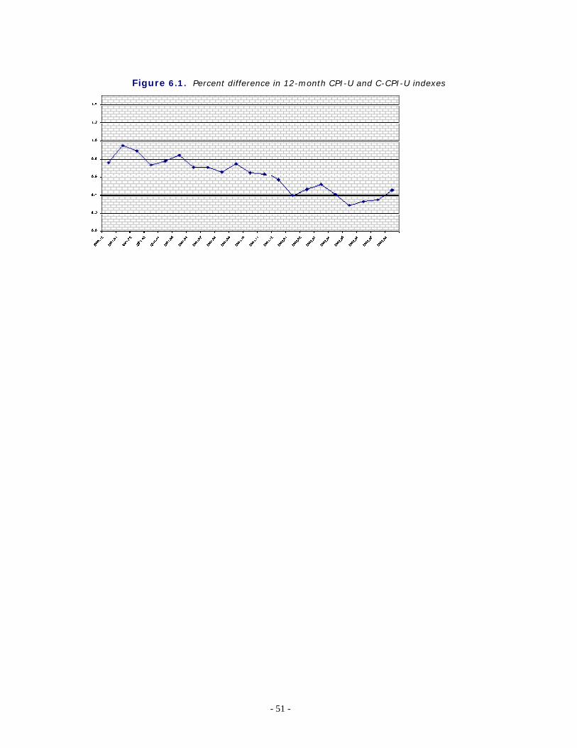
- 51 -

Figure 6.1. Percent difference in 12-month CPI-U and C-CPI-U indexes

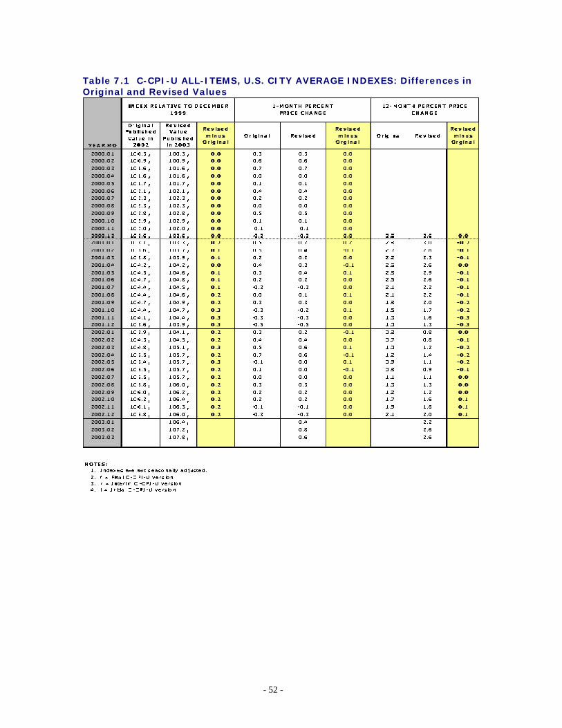
- 52 -

Table 7.1 C-CPI-U ALL-ITEMS, U.S. CITY AVERAGE INDEXES: Differences in Original and Revised Values

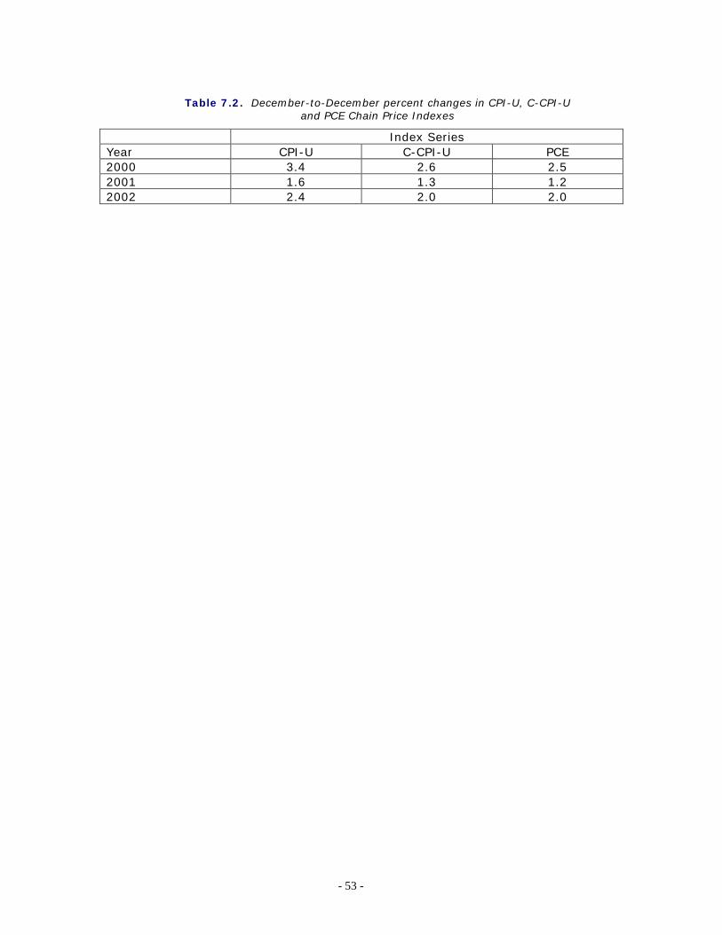
- 53 -

Table 7.2. December-to-December percent changes in CPI-U, C-CPI-U and PCE Chain Price Indexes

Index Series Year CPI-U C-CPI-U PCE 2000 3.4 2.6 2.5 2001 1.6 1.3 1.2 2002 2.4 2.0 2.0