Intro to Stellar Astrophysics L21 The tools of astrophysics ä Virtually all information about the external Universe is received in the form of electromagnetic

Intro to Stellar Astrophysics L2 1

The tools of astrophysicsThe tools of astrophysics

Virtually all information about the external Virtually all information about the external Universe is received in the form of Universe is received in the form of electromagnetic radiationelectromagnetic radiation..

The EM spectrum covers a range >10The EM spectrum covers a range >102020 in in wavelength.wavelength.

The Planck-Einstein relationThe Planck-Einstein relation

implies higher energy = shorter wavelengthimplies higher energy = shorter wavelength

€

E = hf =hc

λ


The EM spectrumThe EM spectrum

*Note*Note: The atmosphere is opaque (or partially so) for radiation : The atmosphere is opaque (or partially so) for radiation in these bands. They can only be observed from high in these bands. They can only be observed from high altitude observatories, balloons, rockets or satellites.altitude observatories, balloons, rockets or satellites. RadioRadio

MillimetreMillimetre MicrowaveMicrowave Infrared* Infrared* VisibleVisible Ultraviolet*Ultraviolet* X-rays*X-rays* -rays*-rays*


Different ‘astronomies’Different ‘astronomies’

Astronomy/Astrophysics today gathers its information Astronomy/Astrophysics today gathers its information from across the EM spectrum, but we still sometimes from across the EM spectrum, but we still sometimes talk about different ‘astronomies’ (optical astronomy, talk about different ‘astronomies’ (optical astronomy, radio astronomy, X-ray astronomy) becauseradio astronomy, X-ray astronomy) because

Atmospheric transmission variesAtmospheric transmission varies Telescopes and detector varyTelescopes and detector vary Different parts of the spectrum reveal different objects Different parts of the spectrum reveal different objects

and different kinds of information…..and different kinds of information…..


For example …For example …

M104 Sombrero GalaxyM104 Sombrero Galaxy..

© NASA/HST and Spitzer

HST visible

Spitzer IR

3.6 (blue), 4.5 (green), 5.8 (orange), and 8.0 (red) m

Combined - HST visible (blue-cyan),

Spitzer 3.6-4.5 m (green) and 8.0 m ( red)


Milky Way at many wavelengthsMilky Way at many wavelengths

© NASA ADF - http://adc.gsfc.nasa.gov/mw/mmw_sci.html


TelescopesTelescopes

Telescopes at many Telescopes at many wavelengths are wavelengths are basically similar. basically similar. Important factors are:Important factors are:

Configuration - Configuration - lens/mirror, lens/mirror, paraboloids, prime paraboloids, prime focus, cassegrain, focus, cassegrain, grazing incidence…grazing incidence…


Telescopes - 2Telescopes - 2

Surface materials - glass, metal sheet, chicken wire,..Surface materials - glass, metal sheet, chicken wire,.. Surface accuracy - ‘diffraction limited’ is < Surface accuracy - ‘diffraction limited’ is < /8 (p-p /8 (p-p

in the surface) or in the surface) or /4 in the wavefront /4 in the wavefront Magnification - not very importantMagnification - not very important Collecting area - light gathering power (sensitivity) Collecting area - light gathering power (sensitivity)

D D2 2 with possiblewith possible ‘secondary obstruction’‘secondary obstruction’


W.M. Keck Observatory - Hawai’iW.M. Keck Observatory - Hawai’i

© NASA/JPL-Caltech


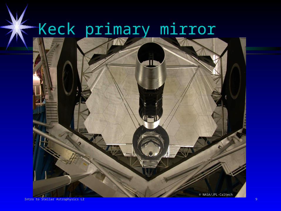
Keck primary mirrorKeck primary mirror

© NASA/JPL-Caltech


Parkes radio telescopeParkes radio telescope

© CSIRO/ATNF ?


SensitivitySensitivity

Factors affecting sensitivity:Factors affecting sensitivity: Atmospheric transmissionAtmospheric transmission Collecting areaCollecting area System throughputSystem throughput Detector quantum efficiencyDetector quantum efficiency Observing timeObserving time Background - e.g. scattered light. As well as natural Background - e.g. scattered light. As well as natural

sources, man-made pollution is a major problem for sources, man-made pollution is a major problem for astronomy. At optical wavelengths for example….astronomy. At optical wavelengths for example….


Light pollutionLight pollution

© unknown

QuickTime™ and aYUV420 codec decompressor

are needed to see this picture.

© Pearson Education 2007


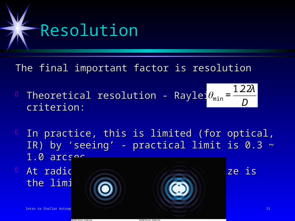
ResolutionResolution

The final important factor is resolution The final important factor is resolution

Theoretical resolution - Rayleigh’s criterion:Theoretical resolution - Rayleigh’s criterion:

In practice, this is limited (for optical, IR) by ‘seeing’ - In practice, this is limited (for optical, IR) by ‘seeing’ - practical limit is 0.3 ~ 1.0 arcsec.practical limit is 0.3 ~ 1.0 arcsec.

At radio wavelengths, telescope size is the limiting factor.At radio wavelengths, telescope size is the limiting factor.€

θmin =1.22λ

D


Resolution - single telescopesResolution - single telescopes

BandBand /8/8 ResolutionResolution TypicalTypical min.surfacemin.surface for D=10 m actual telescopesfor D=10 m actual telescopes

accuracy accuracy

UVUV 100 nm 100 nm 13 nm13 nm 0.0025” 0.010” 0.0025” 0.010” (HST 2.4 m)(HST 2.4 m)

OpticalOptical 500 nm 500 nm 63 nm63 nm 0.013” 0.013” (Keck 10 m)(Keck 10 m)

Near IR 2 Near IR 2 mm 250 nm250 nm 0.050” 0.050” (Keck 10 m)(Keck 10 m)

mmmm 1 mm 1 mm 0.13 mm0.13 mm 25” 25” (JCMT 10 m)(JCMT 10 m)

cmcm 21 cm 21 cm 26 mm26 mm 1.5°1.5° 9’ 9’ (Greenbank 100m)(Greenbank 100m)

Now, concentrating on the optical for a moment…….Now, concentrating on the optical for a moment…….


Adaptive opticsAdaptive optics

Active OpticsActive Optics: : slow image correction (f < 1 Hz), to correct mirror and slow image correction (f < 1 Hz), to correct mirror and

structural deflectionsstructural deflections

Adaptive OpticsAdaptive Optics: : fast image correction (f ≥ 1 Hz), primarily to correct random fast image correction (f ≥ 1 Hz), primarily to correct random

phase fluctuations of wavefronts caused by atmospheric phase fluctuations of wavefronts caused by atmospheric turbulence - resulting image motion and blurringturbulence - resulting image motion and blurring


Where does Seeing arise?Where does Seeing arise?

Turbulence in the atmosphere Turbulence in the atmosphere leads to refractive index variations.leads to refractive index variations.Contributions are concentrated Contributions are concentrated into layers at different altitudes.into layers at different altitudes.

© John O’Byrne


QuickTime™ and aGIF decompressor

are needed to see this picture.

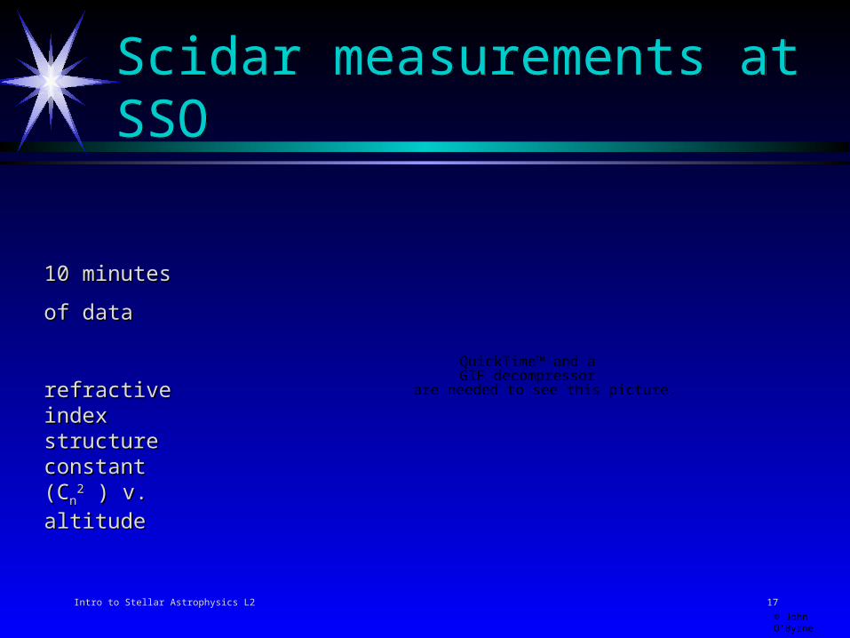
10 minutes 10 minutes

of data of data

refractive index refractive index structure structure constant (Cconstant (Cnn

22 ) )

v. altitudev. altitude

Scidar measurements at SSOScidar measurements at SSO

© John O’Byrne


Seeing parametersSeeing parameters

Fried parameter rFried parameter roo((z) = 0.185 z) = 0.185 6/56/5coscos3/5 3/5 z(∫ Cz(∫ Cnn22dh)dh)-3/5-3/5

Seeing disk FWHM without AO ≈ Seeing disk FWHM without AO ≈ /r/ro o for large for large

telescopestelescopes

So at ~500nm, rSo at ~500nm, roo ≈ 10 cm ≈ 10 cm for for 1 arcsec FWHM seeing 1 arcsec FWHM seeing

At 2.5 At 2.5 m, this corresponds to rm, this corresponds to roo ≈ 70 cm ≈ 70 cm and and

0.7 0.7 arcsec seeing arcsec seeing


Essentials of an AO systemEssentials of an AO system

Wavefront sensorWavefront sensor ComputerComputer Phase modulatorPhase modulator

© John O’Byrne


AO exampleAO example

© University of Hawaii ?


Keck - IoKeck - Io

Upper Left:Upper Left:

Keck AO; K-band, Keck AO; K-band, 2.2micron.2.2micron.

Upper Right:Upper Right:

Galileo; visible light.Galileo; visible light. Lower Left:Lower Left:

Keck AO; L-band, Keck AO; L-band, 3.5micron.3.5micron.

Lower Right:Lower Right:

Keck without adaptive Keck without adaptive optics.optics.

© NASA/JPL-Caltech


InterferometryInterferometry

If EM waves from two or more apertures are If EM waves from two or more apertures are coherently coherently combined, the resolution is set by the “baseline” combined, the resolution is set by the “baseline” BB between the between the apertures.apertures.

Interferometry first proposed by Fizeau but first successful Interferometry first proposed by Fizeau but first successful astronomical interferometer was due to Michelson (1891 astronomical interferometer was due to Michelson (1891 Galilean satellites).Galilean satellites).

In 1921 Michelson & Pease measured angular diameter of In 1921 Michelson & Pease measured angular diameter of Orionis (Betelgeuse). Orionis (Betelgeuse).

1950s: Discovered by radio astronomers!1950s: Discovered by radio astronomers! Now widely used in radio, difficult at optical/IR.Now widely used in radio, difficult at optical/IR.


Basic principle of an optical interferometer - the Basic principle of an optical interferometer - the Sydney University Stellar Interferometer (SUSI) Sydney University Stellar Interferometer (SUSI) at Narrabri is a 2-dimensional exampleat Narrabri is a 2-dimensional example

© University of Sydney


Resolution - interferometersResolution - interferometers

BaselineBaselineResolutionResolution

TypicalTypical max.max.

SUSI 400 nmSUSI 400 nm 640 m640 m 0.0002”0.0002”ATCAATCA 6 cm 6 cm ~20 km~20 km 2.5”2.5”VLBI 6 cmVLBI 6 cm ~5000 km~5000 km 0.003”0.003”

© CSIRO/ATNF

Documents

Intro to Stellar Astrophysics L21 The tools of astrophysics ä Virtually all information about the external Universe is received in the form of electromagnetic