Embed Size (px)
Citation preview
Intro to Neural NetworksPart 1: What is a neural network
Lisbon Machine Learning School
July 2017
What’s in this tutorial
• We will learn about
– What is a neural network
– What can neural networks model
– Issues with learning
– Some basic models: CNNs and RNNs

Instructor
• Bhiksha Raj
Professor,Language Technologies InstituteCarnegie Mellon Univ.
Neural Networks are taking over!
• Neural networks have become one of the major thrust areas recently in various pattern recognition, prediction, and analysis problems
• In many problems they have established the state of the art
– Often exceeding previous benchmarks by large margins
Recent success with neural networks
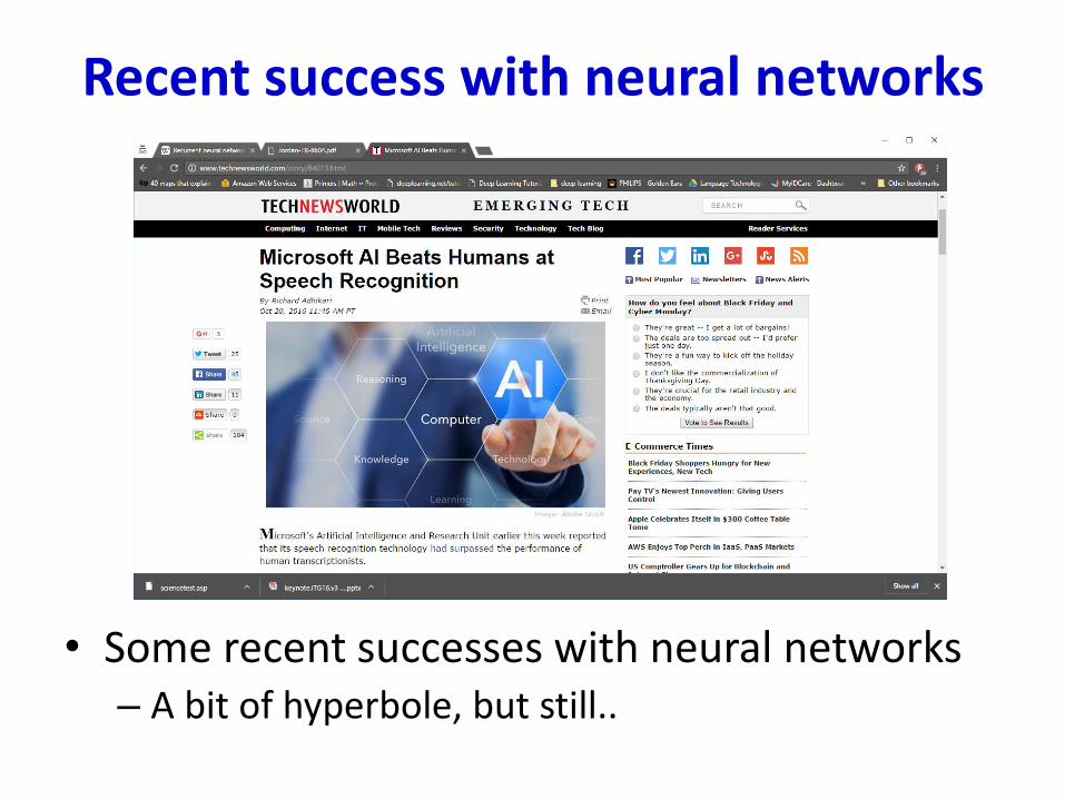
• Some recent successes with neural networks– A bit of hyperbole, but still..
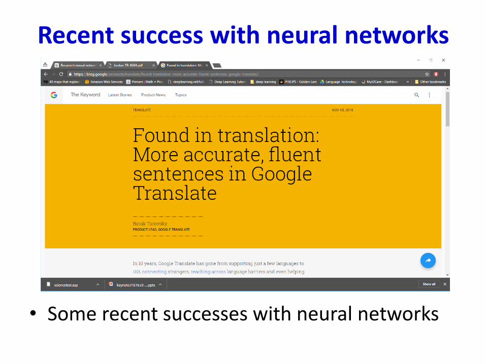
Recent success with neural networks
• Some recent successes with neural networks
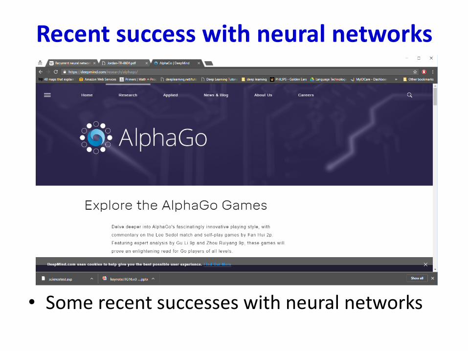
Recent success with neural networks
• Some recent successes with neural networks
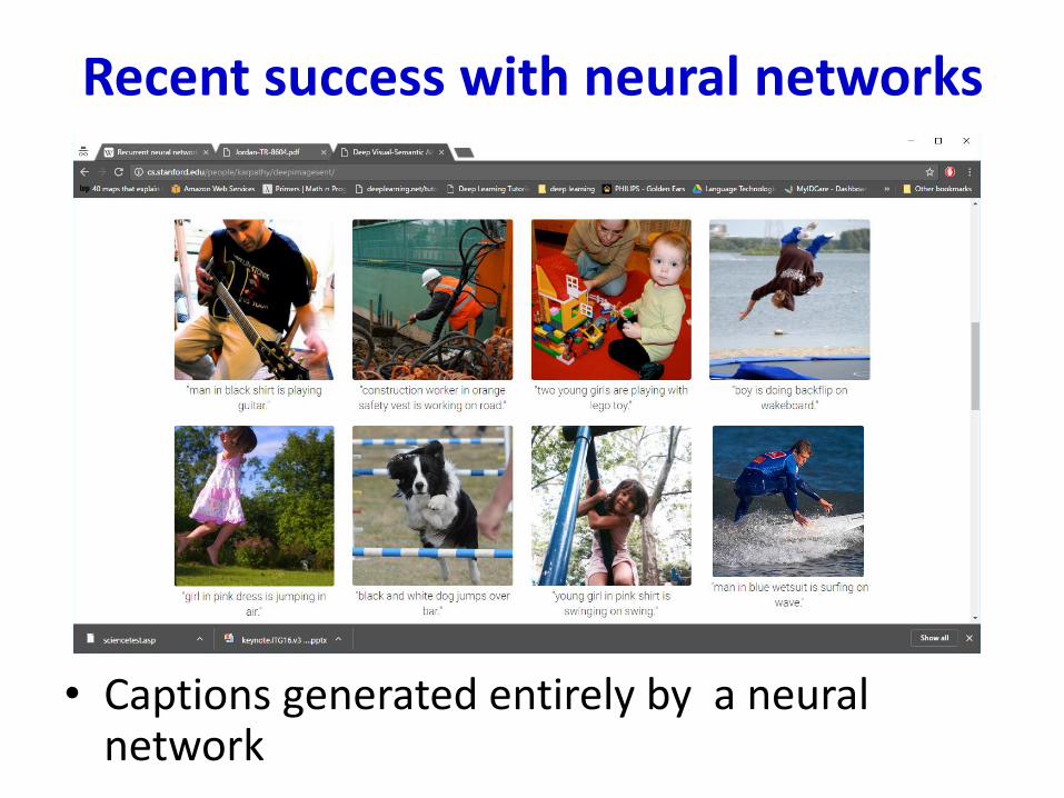
Recent success with neural networks
• Captions generated entirely by a neural network
Successes with neural networks
• And a variety of other problems:
– Image recognition
– Signal enhancement
– Even predicting stock markets!
Neural nets and the employment market
This guy didn’t know about neural networks (a.k.a deep learning)
This guy learned about neural networks (a.k.a deep learning)
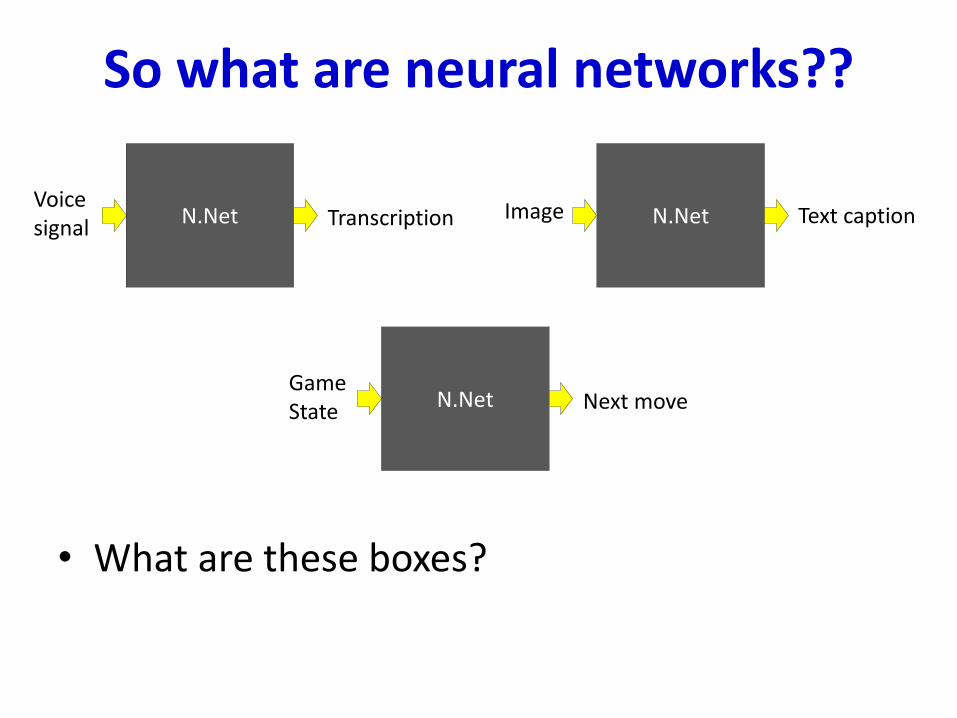
So what are neural networks??
• What are these boxes?
N.NetVoice signal Transcription N.NetImage Text caption
N.NetGameState Next move
So what are neural networks??
• It begins with this..
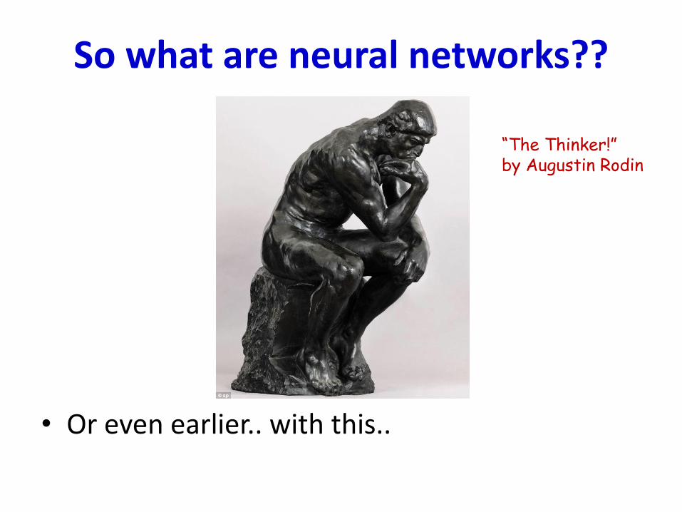
So what are neural networks??
• Or even earlier.. with this..
“The Thinker!”by Augustin Rodin
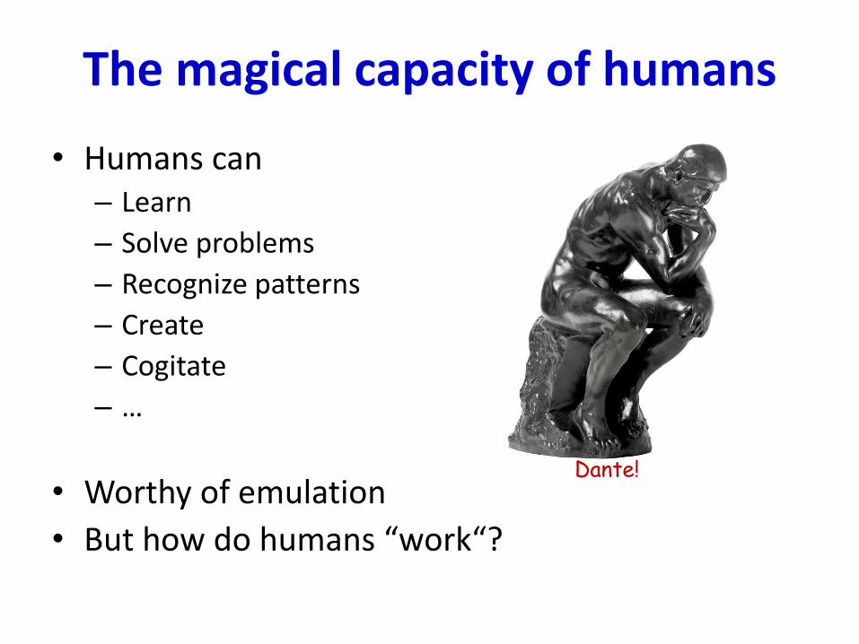
The magical capacity of humans
• Humans can– Learn
– Solve problems
– Recognize patterns
– Create
– Cogitate
– …
• Worthy of emulation
• But how do humans “work“?
Dante!
Cognition and the brain..
• “If the brain was simple enough to be understood - we would be too simple to understand it!”
– Marvin Minsky
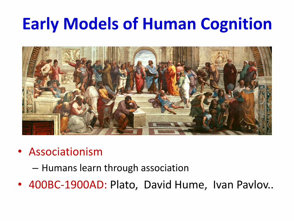
Early Models of Human Cognition
• Associationism
– Humans learn through association
• 400BC-1900AD: Plato, David Hume, Ivan Pavlov..
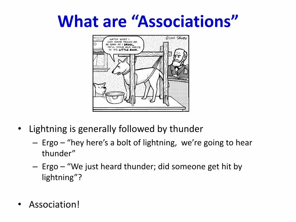
What are “Associations”
• Lightning is generally followed by thunder
– Ergo – “hey here’s a bolt of lightning, we’re going to hear thunder”
– Ergo – “We just heard thunder; did someone get hit by lightning”?
• Association!
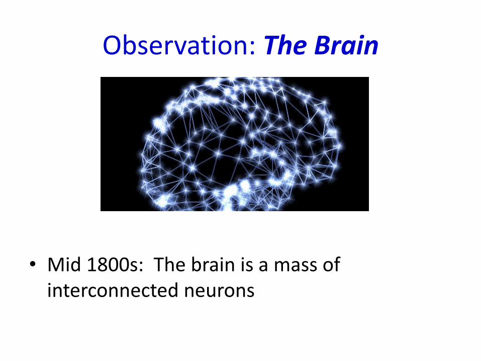
Observation: The Brain
• Mid 1800s: The brain is a mass of interconnected neurons
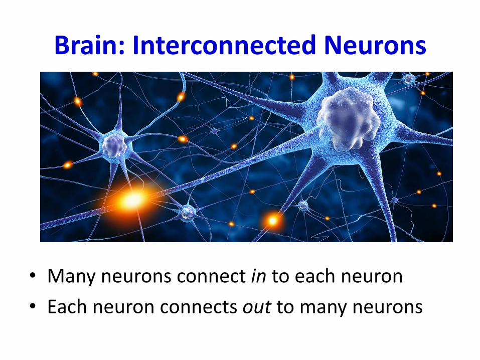
Brain: Interconnected Neurons
• Many neurons connect in to each neuron
• Each neuron connects out to many neurons
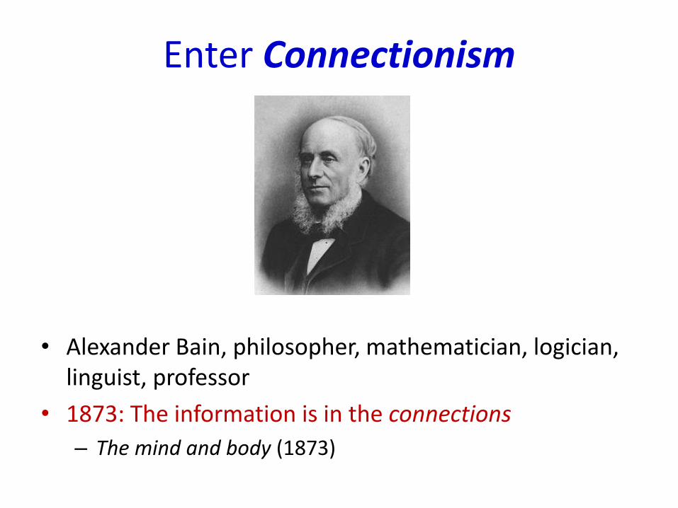
Enter Connectionism
• Alexander Bain, philosopher, mathematician, logician, linguist, professor
• 1873: The information is in the connections
– The mind and body (1873)
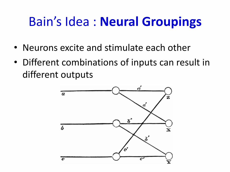
Bain’s Idea : Neural Groupings
• Neurons excite and stimulate each other
• Different combinations of inputs can result in different outputs
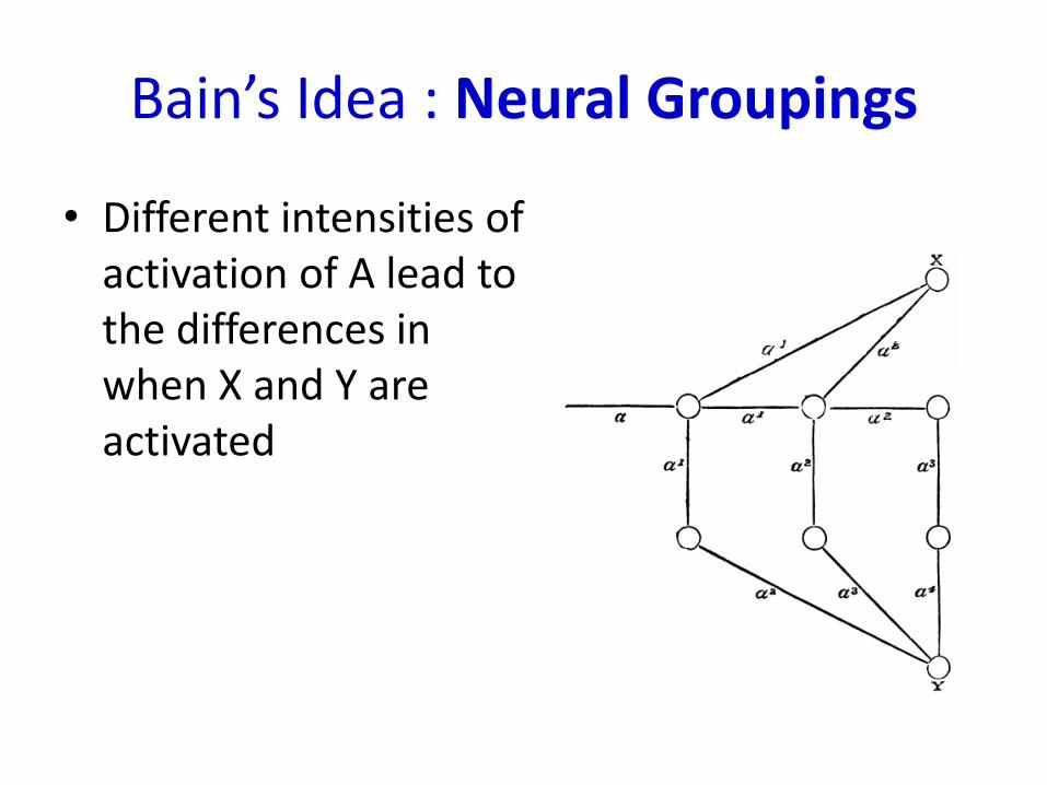
Bain’s Idea : Neural Groupings
• Different intensities of activation of A lead to the differences in when X and Y are activated
Bain’s Idea 2: Making Memories
• “when two impressions concur, or closely succeed one another, the nerve currents find some bridge or place of continuity, better or worse, according to the abundance of nerve matter available for the transition.”
• Predicts “Hebbian” learning (half a century before Hebb!)
Bain’s Doubts
• “The fundamental cause of the trouble is that in the modern world the stupid are cocksure while the intelligent are full of doubt.”
– Bertrand Russell
• In 1873, Bain postulated that there must be one million neurons and 5 billion connections relating to 200,000 “acquisitions”
• In 1883, Bain was concerned that he hadn’t taken into account the number of “partially formed associations” and the number of neurons responsible for recall/learning
• By the end of his life (1903), recanted all his ideas!
– Too complex; the brain would need too many neurons and connections
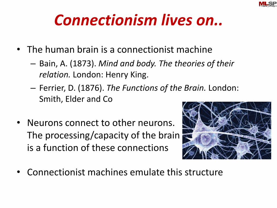
Connectionism lives on..
• The human brain is a connectionist machine
– Bain, A. (1873). Mind and body. The theories of their relation. London: Henry King.
– Ferrier, D. (1876). The Functions of the Brain. London: Smith, Elder and Co
• Neurons connect to other neurons. The processing/capacity of the brain is a function of these connections
• Connectionist machines emulate this structure
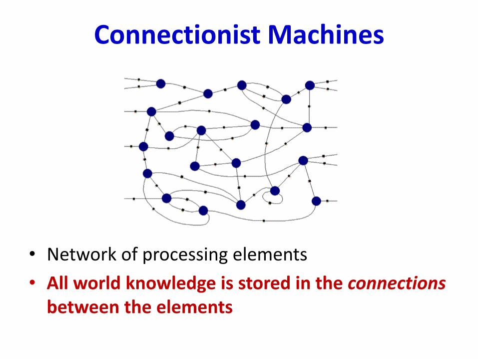
Connectionist Machines
• Network of processing elements
• All world knowledge is stored in the connections between the elements
Connectionist Machines
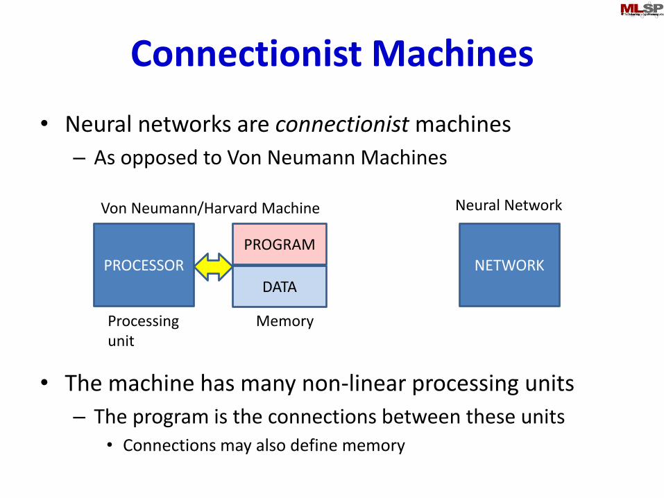
• Neural networks are connectionist machines
– As opposed to Von Neumann Machines
• The machine has many non-linear processing units
– The program is the connections between these units• Connections may also define memory
PROCESSOR
PROGRAM
DATA
MemoryProcessingunit
Von Neumann/Harvard Machine
NETWORK
Neural Network
Recap
• Neural network based AI has taken over most AI tasks
• Neural networks originally began as computational models of the brain
– Or more generally, models of cognition
• The earliest model of cognition was associationism
• The more recent model of the brain is connectionist
– Neurons connect to neurons
– The workings of the brain are encoded in these connections
• Current neural network models are connectionist machines
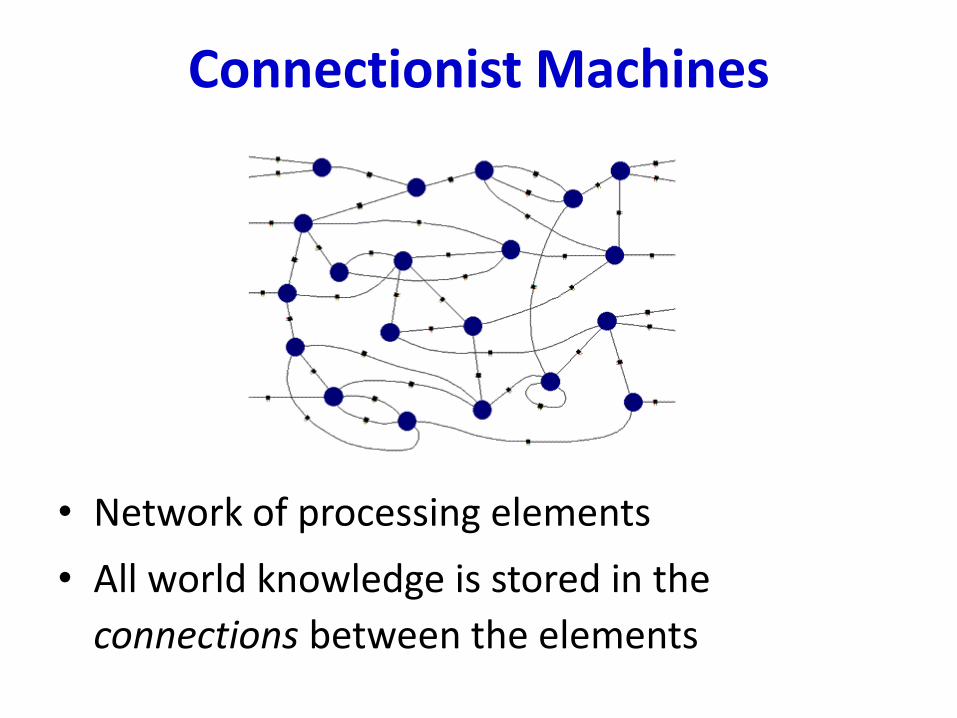
Connectionist Machines
• Network of processing elements
• All world knowledge is stored in the
connections between the elements
Connectionist Machines
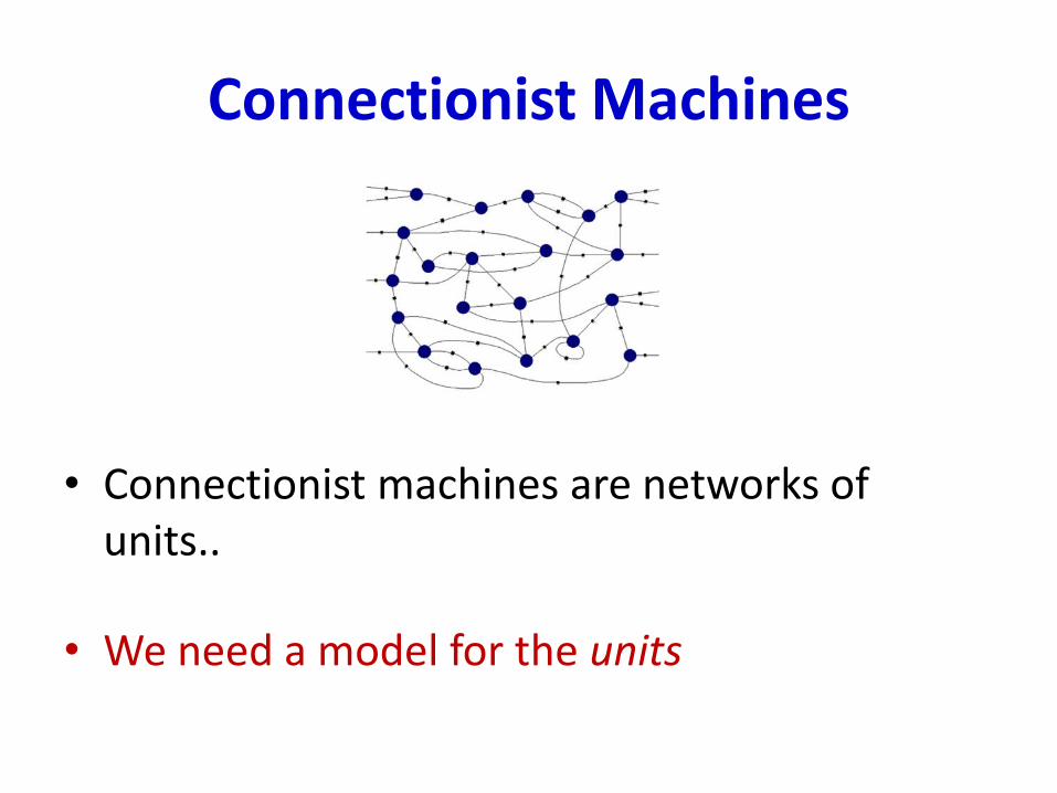
• Connectionist machines are networks of units..
• We need a model for the units
Modelling the brain
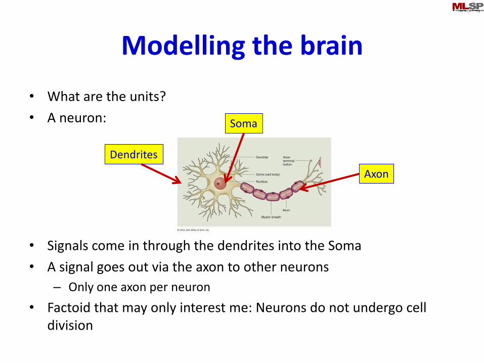
• What are the units?
• A neuron:
• Signals come in through the dendrites into the Soma
• A signal goes out via the axon to other neurons
– Only one axon per neuron
• Factoid that may only interest me: Neurons do not undergo cell division
Dendrites
Soma
Axon
McCullough and Pitts
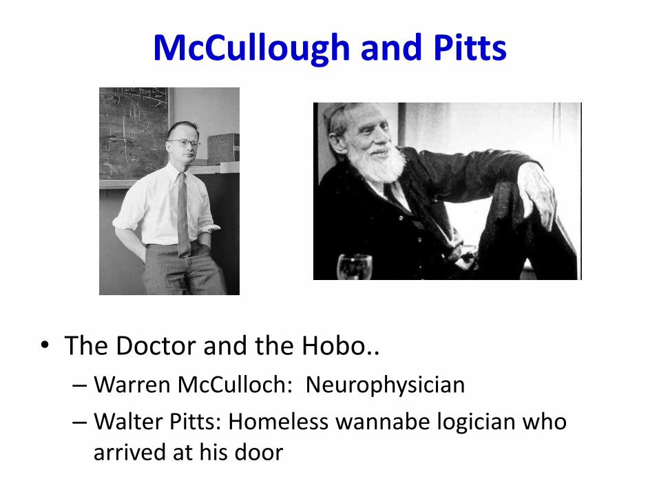
• The Doctor and the Hobo..
– Warren McCulloch: Neurophysician
– Walter Pitts: Homeless wannabe logician who arrived at his door

The McCulloch and Pitts model
• A mathematical model of a neuron
– McCulloch, W.S. & Pitts, W.H. (1943). A Logical Calculus of the Ideas Immanent in Nervous Activity, Bulletin of Mathematical Biophysics, 5:115-137, 1943
• Pitts was only 20 years old at this time
– Threshold Logic
A single neuron
Synaptic Model
• Excitatory synapse: Transmits weighted input to the neuron
• Inhibitory synapse: Any signal from an inhibitory synapse forces output to zero
– The activity of any inhibitory synapse absolutely prevents excitation of the neuron at that time.
• Regardless of other inputs
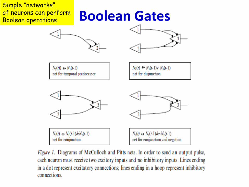
Boolean GatesSimple “networks”of neurons can performBoolean operations
Criticisms
• Several..
– Claimed their machine could emulate a turing
machine
• Didn’t provide a learning mechanism..
Donald Hebb
• “Organization of behavior”, 1949
• A learning mechanism:
– Neurons that fire together wire together
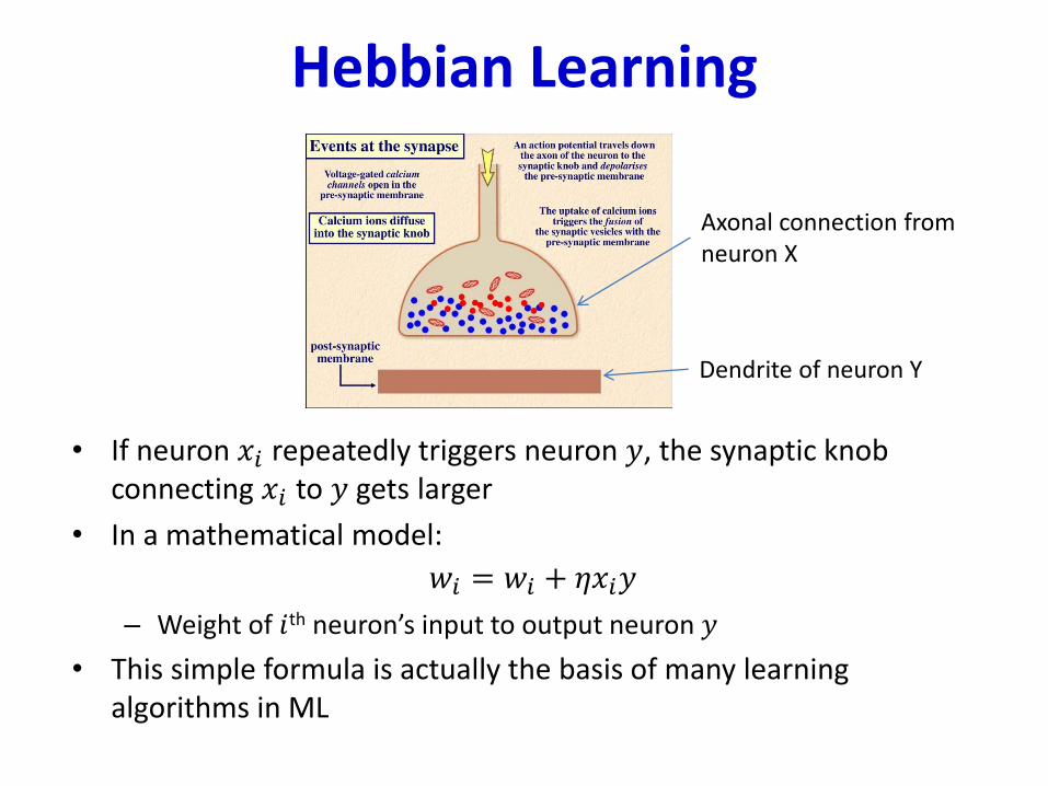
Hebbian Learning
• If neuron 𝑥𝑖 repeatedly triggers neuron 𝑦, the synaptic knob connecting 𝑥𝑖 to 𝑦 gets larger
• In a mathematical model:
𝑤𝑖 = 𝑤𝑖 + 𝜂𝑥𝑖𝑦
– Weight of 𝑖th neuron’s input to output neuron 𝑦
• This simple formula is actually the basis of many learning algorithms in ML
Dendrite of neuron Y
Axonal connection fromneuron X
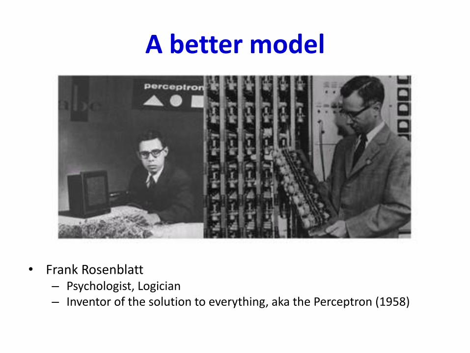
A better model
• Frank Rosenblatt– Psychologist, Logician– Inventor of the solution to everything, aka the Perceptron (1958)

Simplified mathematical model
• Number of inputs combine linearly
– Threshold logic: Fire if combined input exceeds
threshold
𝑌 = ൞1 𝑖𝑓
𝑖
𝑤𝑖𝑥𝑖 + 𝑏 > 0
0 𝑒𝑙𝑠𝑒
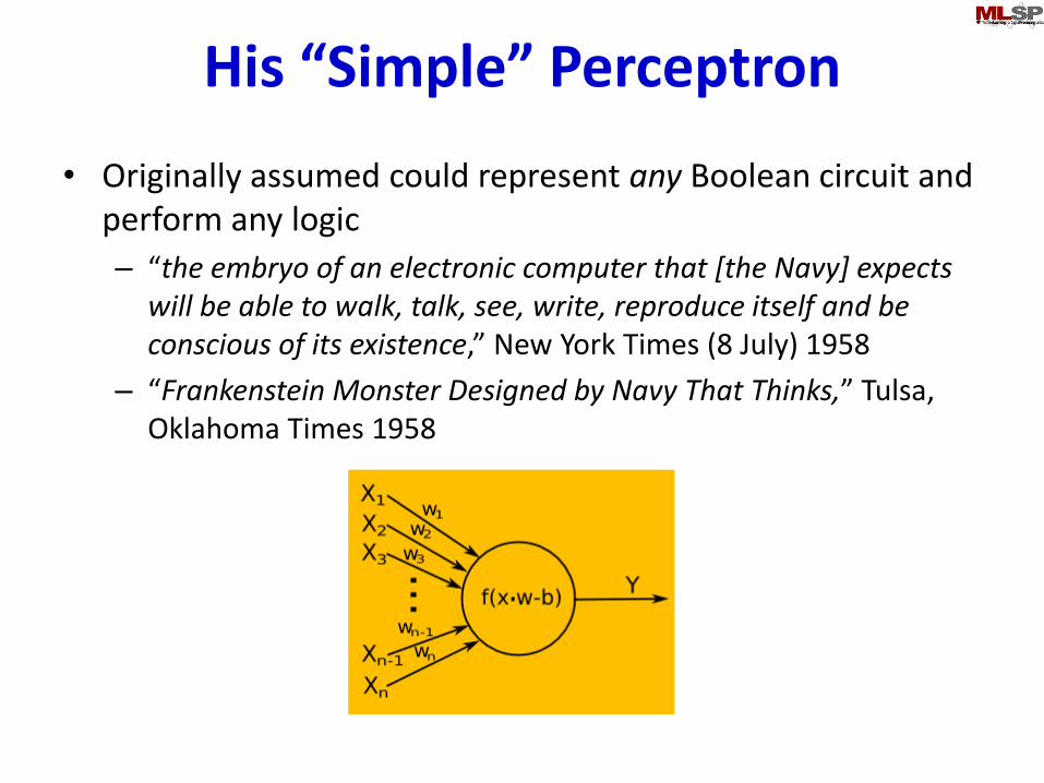
His “Simple” Perceptron
• Originally assumed could represent any Boolean circuit and perform any logic
– “the embryo of an electronic computer that [the Navy] expects will be able to walk, talk, see, write, reproduce itself and be conscious of its existence,” New York Times (8 July) 1958
– “Frankenstein Monster Designed by Navy That Thinks,” Tulsa, Oklahoma Times 1958
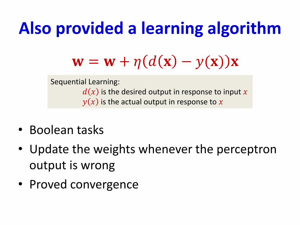
Also provided a learning algorithm
• Boolean tasks
• Update the weights whenever the perceptron output is wrong
• Proved convergence
𝐰 = 𝐰+ 𝜂 𝑑 𝐱 − 𝑦(𝐱) 𝐱Sequential Learning:
𝑑 𝑥 is the desired output in response to input 𝑥𝑦 𝑥 is the actual output in response to 𝑥
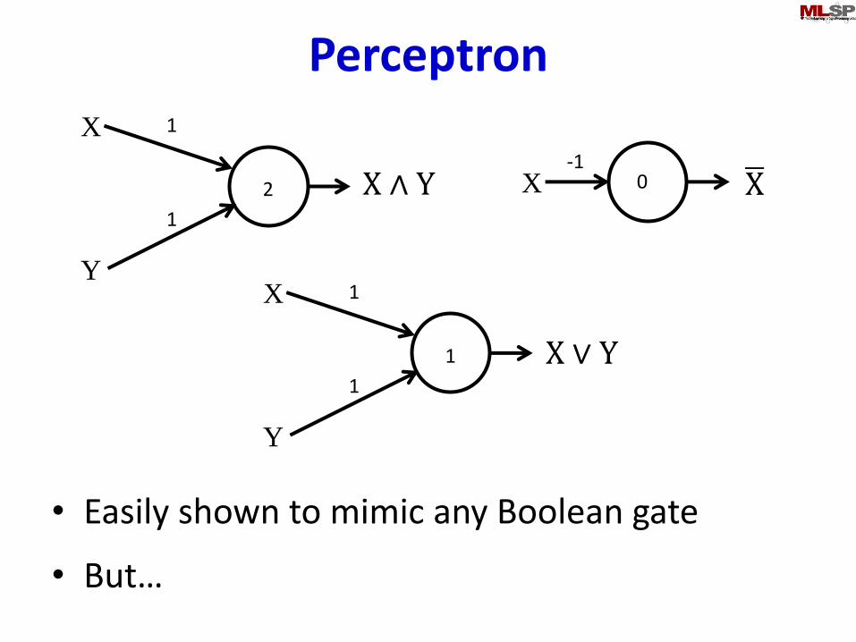
Perceptron
• Easily shown to mimic any Boolean gate
• But…
X
Y
1
1
2
X
Y
1
1
1
0X-1
X ∧ Y
X ∨ Y
ഥX
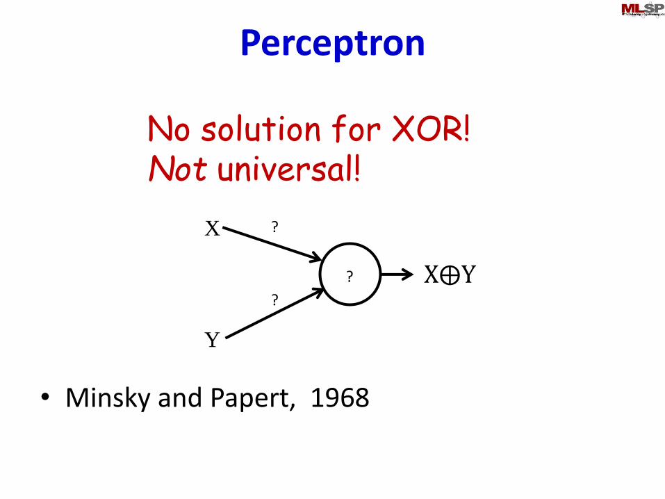
Perceptron
X
Y
?
?
? X⨁Y
No solution for XOR!Not universal!
• Minsky and Papert, 1968
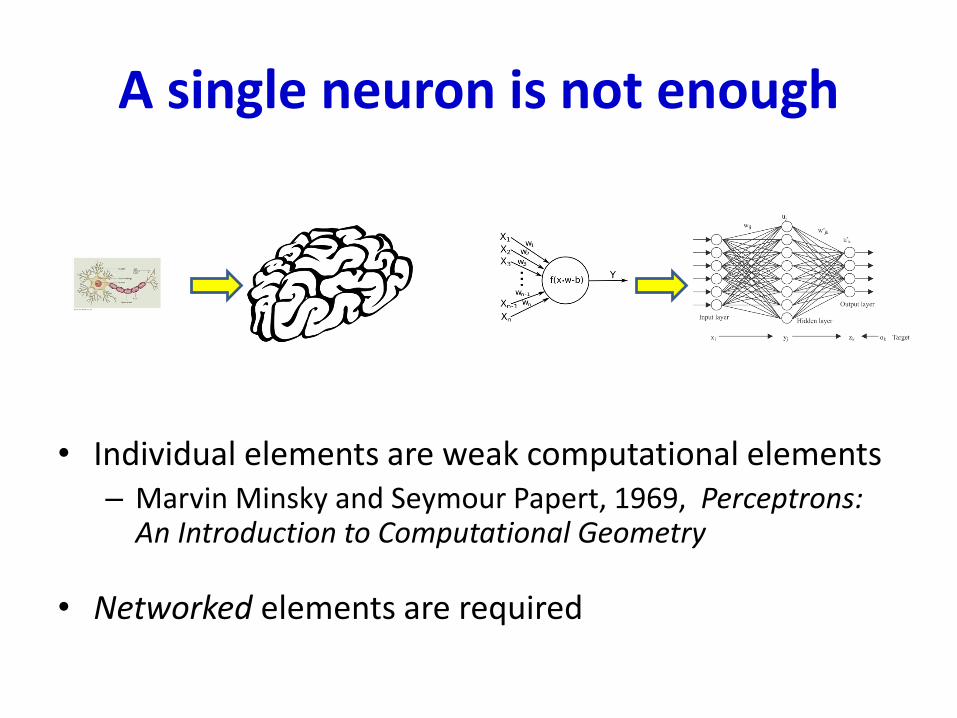
A single neuron is not enough
• Individual elements are weak computational elements– Marvin Minsky and Seymour Papert, 1969, Perceptrons:
An Introduction to Computational Geometry
• Networked elements are required
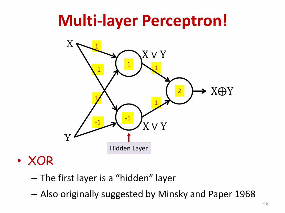
Multi-layer Perceptron!
• XOR
– The first layer is a “hidden” layer
– Also originally suggested by Minsky and Paper 196846
1
1
1
-1
1
-1
X
Y
1
X⨁Y
-1
2
X ∨ Y
ഥX ∨ ഥY
Hidden Layer
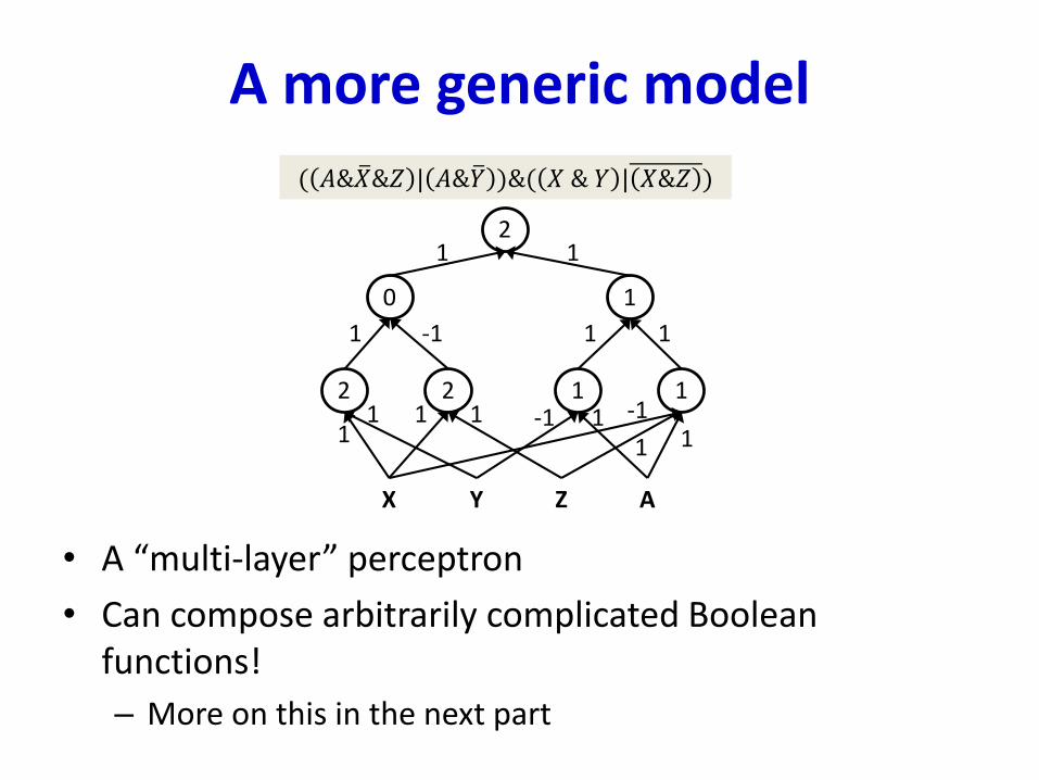
A more generic model
• A “multi-layer” perceptron
• Can compose arbitrarily complicated Boolean functions!
– More on this in the next part
( 𝐴& ത𝑋&𝑍 | 𝐴& ത𝑌 )&( 𝑋 & 𝑌 | 𝑋&𝑍 )
12 1 1 12 1 1
X Y Z A
10 11
12
11 1-111 -1
1 1
1 -1 1 1
11
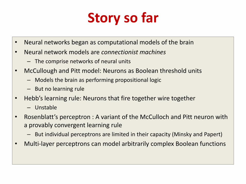
Story so far
• Neural networks began as computational models of the brain
• Neural network models are connectionist machines
– The comprise networks of neural units
• McCullough and Pitt model: Neurons as Boolean threshold units
– Models the brain as performing propositional logic
– But no learning rule
• Hebb’s learning rule: Neurons that fire together wire together
– Unstable
• Rosenblatt’s perceptron : A variant of the McCulloch and Pitt neuron with a provably convergent learning rule
– But individual perceptrons are limited in their capacity (Minsky and Papert)
• Multi-layer perceptrons can model arbitrarily complex Boolean functions
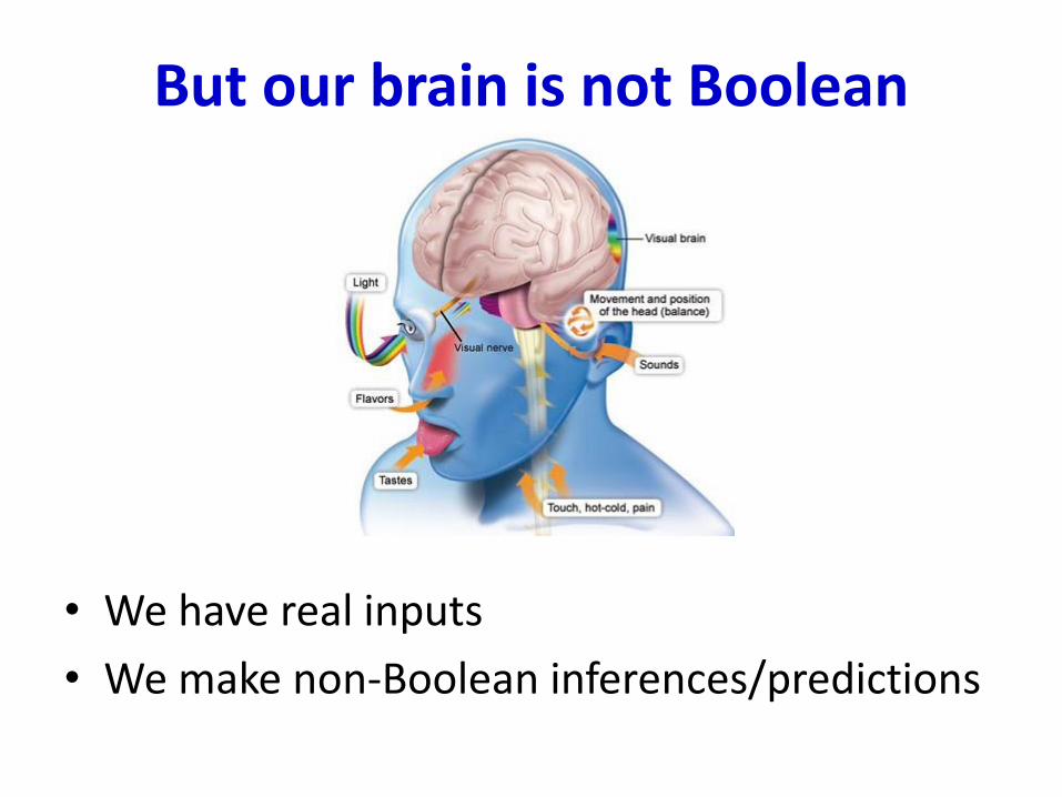
But our brain is not Boolean
• We have real inputs
• We make non-Boolean inferences/predictions
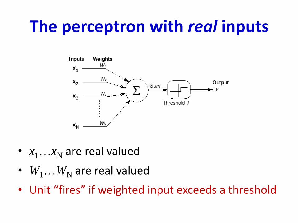
The perceptron with real inputs
• x1…xN are real valued
• W1…WN are real valued
• Unit “fires” if weighted input exceeds a threshold
x1
x2
x3
xN
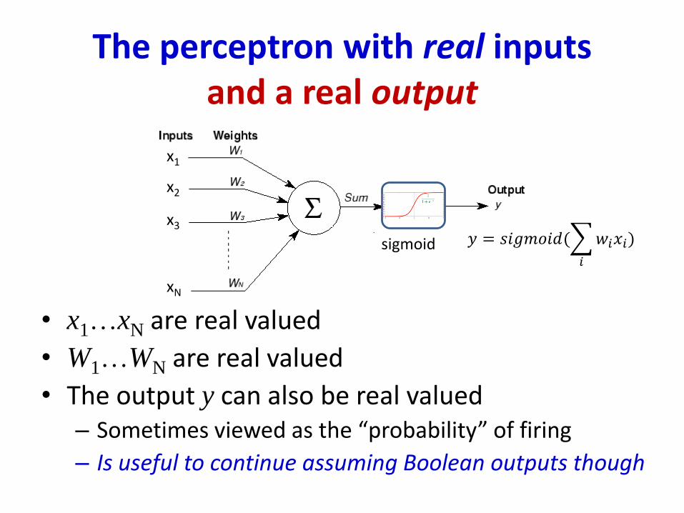
The perceptron with real inputsand a real output
• x1…xN are real valued
• W1…WN are real valued
• The output y can also be real valued– Sometimes viewed as the “probability” of firing
– Is useful to continue assuming Boolean outputs though
sigmoid 𝑦 = 𝑠𝑖𝑔𝑚𝑜𝑖𝑑(
𝑖
𝑤𝑖𝑥𝑖)
x1
x2
x3
xN
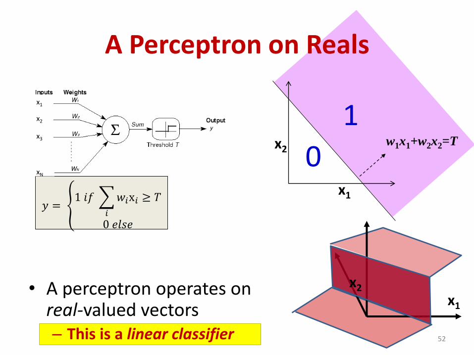
A Perceptron on Reals
• A perceptron operates on real-valued vectors– This is a linear classifier 52
x1
x2w1x1+w2x2=T
𝑦 = ൞1 𝑖𝑓
𝑖
𝑤𝑖x𝑖 ≥ 𝑇
0 𝑒𝑙𝑠𝑒
x1
x2
1
0
x1
x2
x3
xN
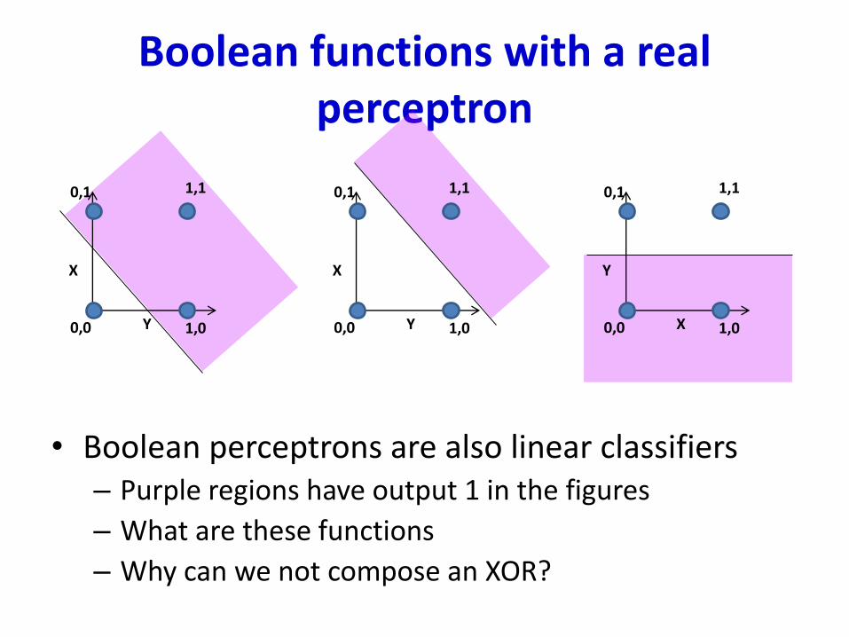
Boolean functions with a real perceptron
• Boolean perceptrons are also linear classifiers– Purple regions have output 1 in the figures
– What are these functions
– Why can we not compose an XOR?
Y
X
0,0
0,1
1,0
1,1
Y
X
0,0
0,1
1,0
1,1
X
Y
0,0
0,1
1,0
1,1
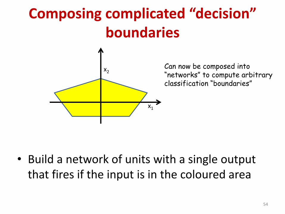
Composing complicated “decision” boundaries
• Build a network of units with a single output that fires if the input is in the coloured area
54
x1
x2Can now be composed into“networks” to compute arbitraryclassification “boundaries”
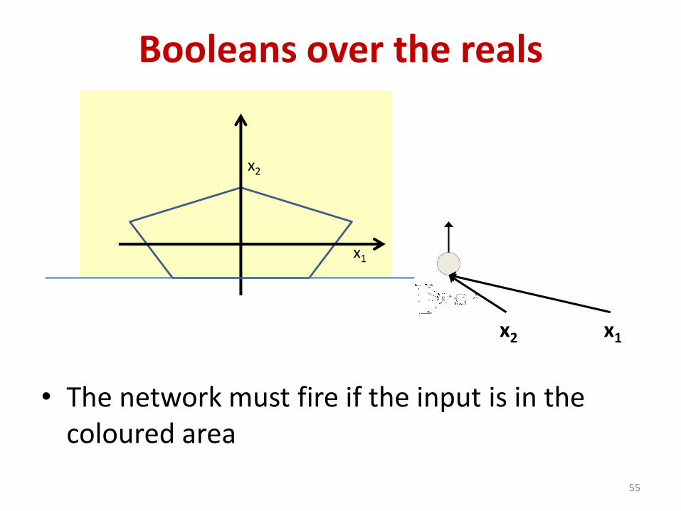
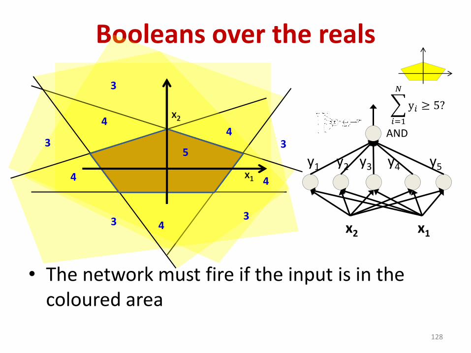
Booleans over the reals
• The network must fire if the input is in the coloured area
55
x1
x2
x1x2
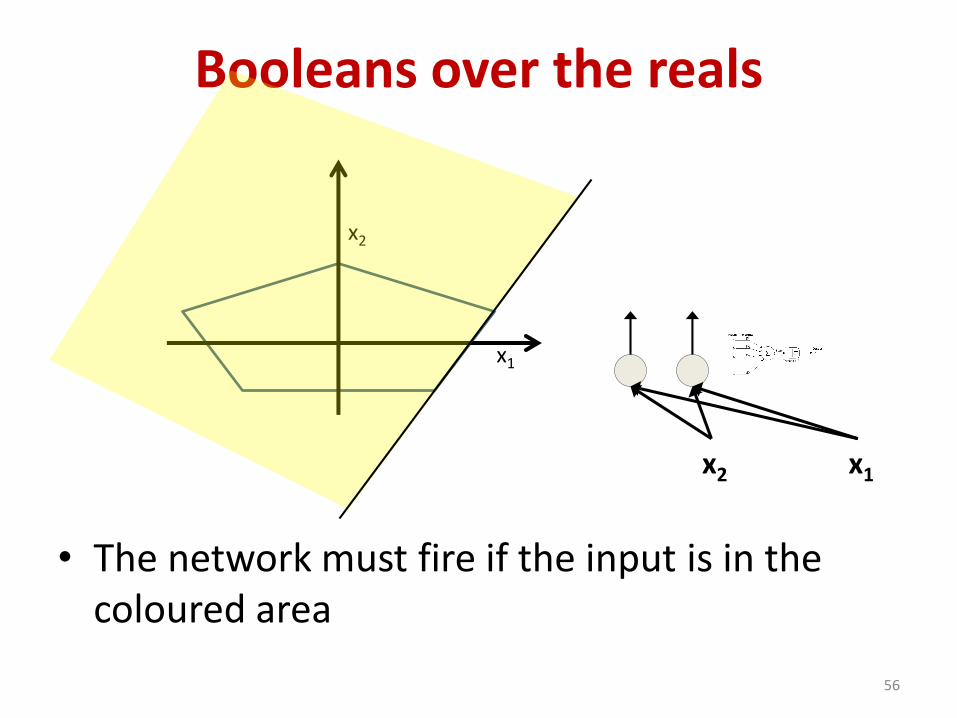
Booleans over the reals
• The network must fire if the input is in the coloured area
56
x1
x2
x1x2
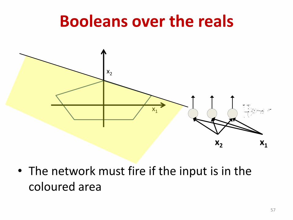
Booleans over the reals
• The network must fire if the input is in the coloured area
57
x1
x2
x1x2
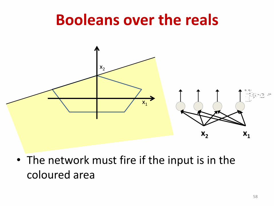
Booleans over the reals
• The network must fire if the input is in the coloured area
58
x1
x2
x1x2
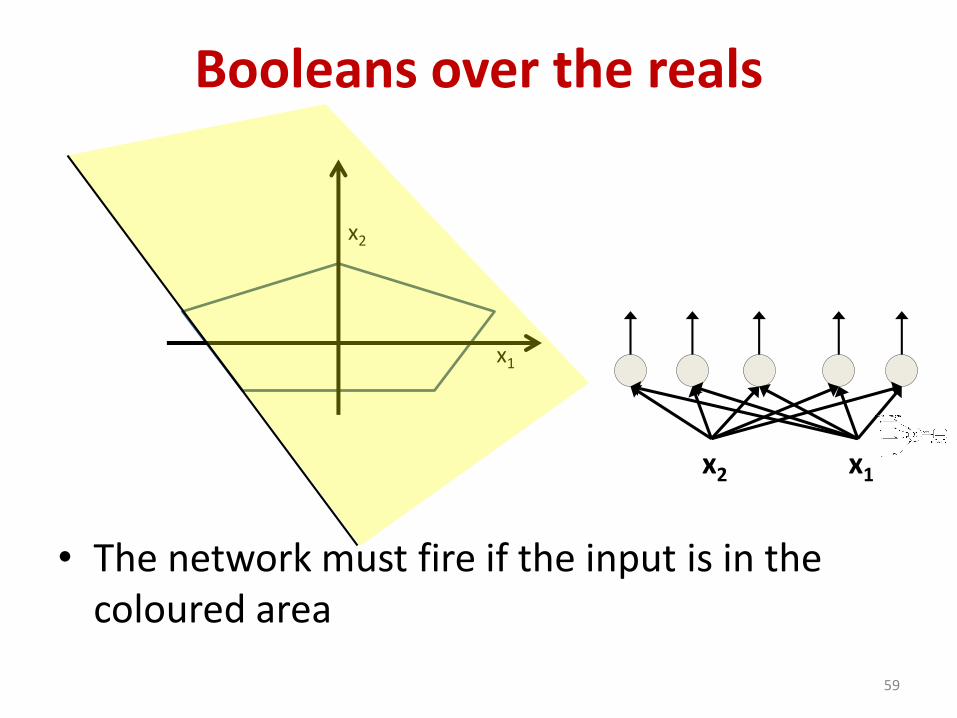
Booleans over the reals
• The network must fire if the input is in the coloured area
59
x1
x2
x1x2

Booleans over the reals
• The network must fire if the input is in the coloured area
60
x1
x2
x1
x2
AND
5
44
4
4
4
3
3
3
33 x1x2
𝑖=1
𝑁
y𝑖 ≥ 5?
y1 y5y2 y3 y4

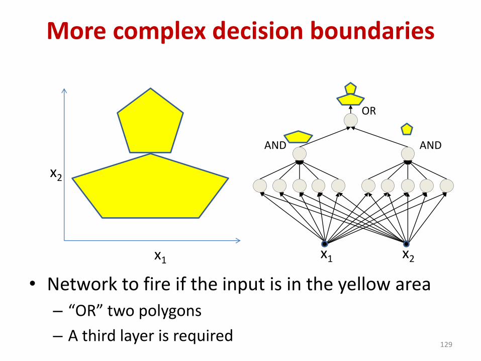
More complex decision boundaries
• Network to fire if the input is in the yellow area
– “OR” two polygons
– A third layer is required61
x2
AND AND
OR
x1 x1 x2
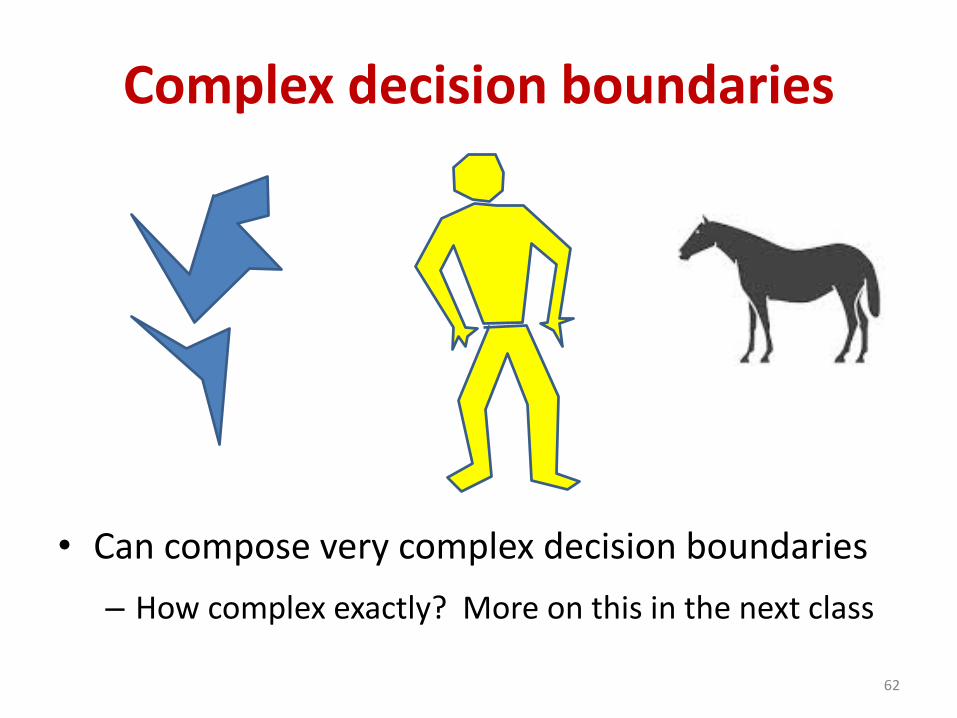
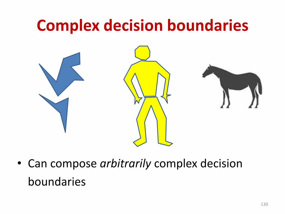
Complex decision boundaries
• Can compose very complex decision boundaries
– How complex exactly? More on this in the next class
62
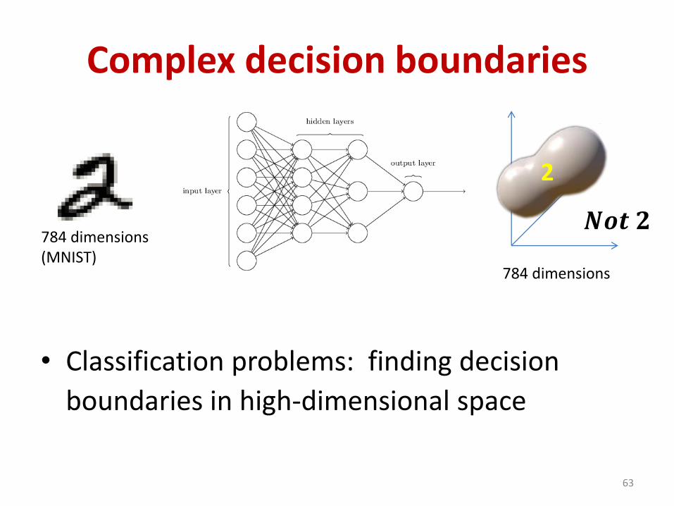
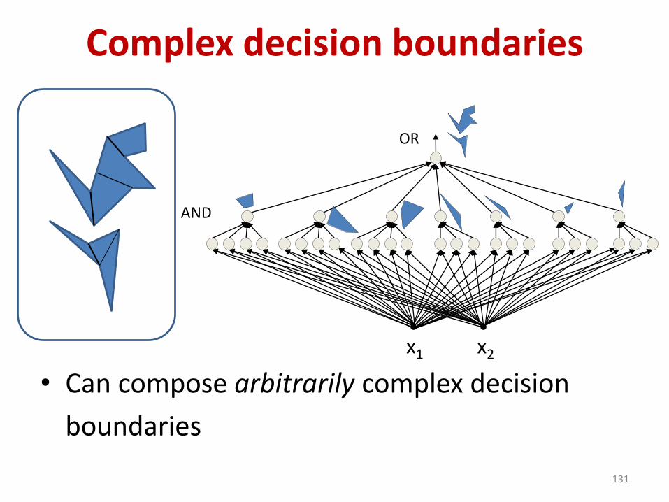
Complex decision boundaries
• Classification problems: finding decision
boundaries in high-dimensional space
63
784 dimensions(MNIST)
784 dimensions
2
𝑵𝒐𝒕 𝟐
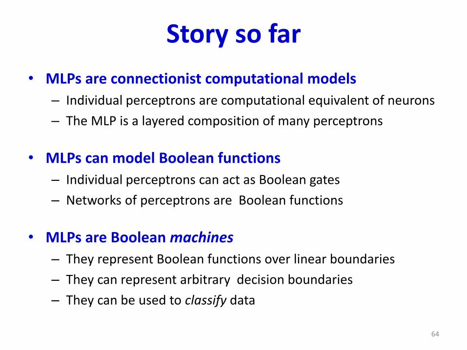
Story so far
• MLPs are connectionist computational models
– Individual perceptrons are computational equivalent of neurons
– The MLP is a layered composition of many perceptrons
• MLPs can model Boolean functions
– Individual perceptrons can act as Boolean gates
– Networks of perceptrons are Boolean functions
• MLPs are Boolean machines
– They represent Boolean functions over linear boundaries
– They can represent arbitrary decision boundaries
– They can be used to classify data
64
So what does the perceptron really model?
• Is there a “semantic” interpretation?
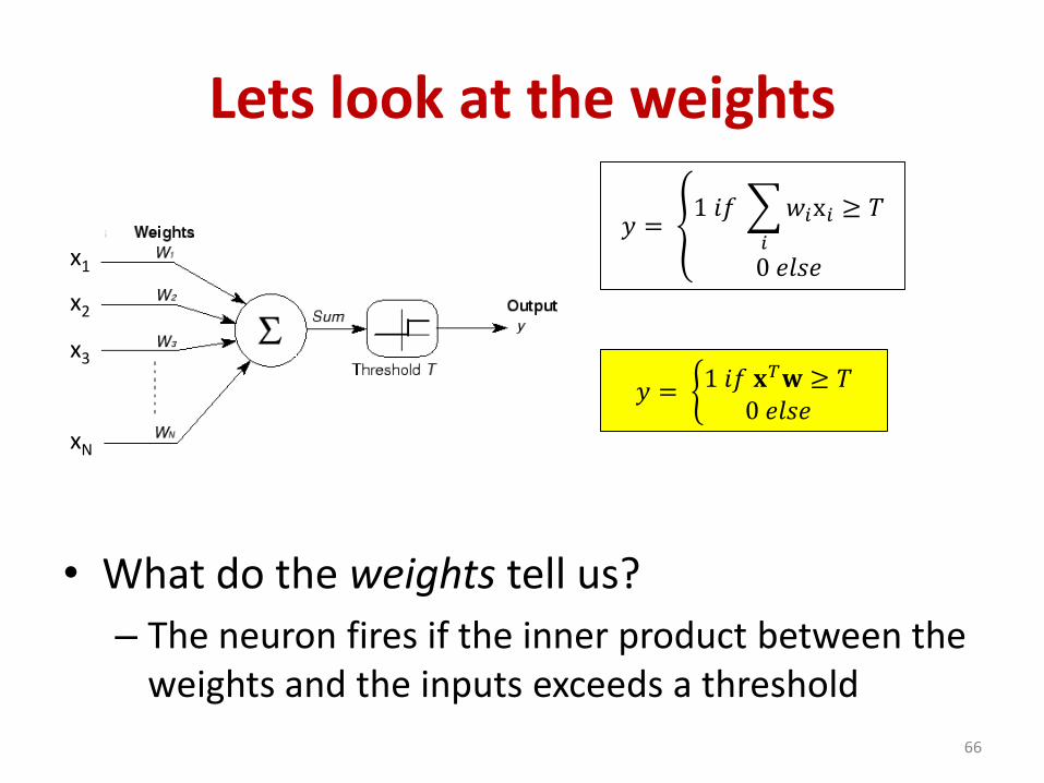
Lets look at the weights
• What do the weights tell us?
– The neuron fires if the inner product between the weights and the inputs exceeds a threshold
66
x1
x2
x3
xN
𝑦 = ൞1 𝑖𝑓
𝑖
𝑤𝑖x𝑖 ≥ 𝑇
0 𝑒𝑙𝑠𝑒
𝑦 = ቊ1 𝑖𝑓 𝐱𝑇𝐰 ≥ 𝑇
0 𝑒𝑙𝑠𝑒
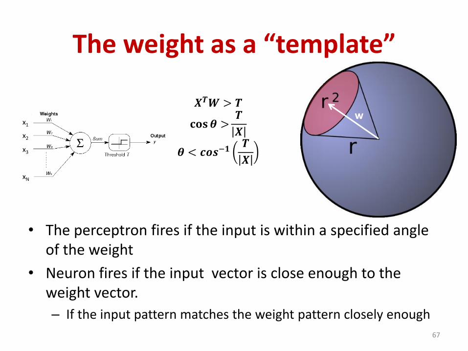
The weight as a “template”
• The perceptron fires if the input is within a specified angle of the weight
• Neuron fires if the input vector is close enough to the weight vector.
– If the input pattern matches the weight pattern closely enough
67
w𝑿𝑻𝑾 > 𝑻
𝐜𝐨𝐬𝜽 >𝑻
𝑿
𝜽 < 𝒄𝒐𝒔−𝟏𝑻
𝑿
x1
x2
x3
xN
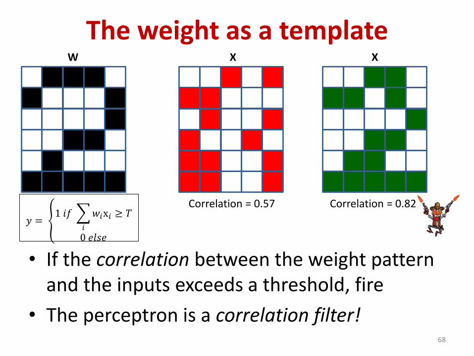
The weight as a template
• If the correlation between the weight pattern and the inputs exceeds a threshold, fire
• The perceptron is a correlation filter!68
W X X
Correlation = 0.57 Correlation = 0.82
𝑦 = ൞1 𝑖𝑓
𝑖
𝑤𝑖x𝑖 ≥ 𝑇
0 𝑒𝑙𝑠𝑒
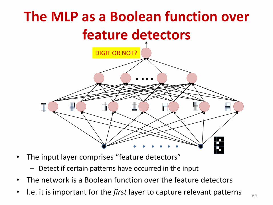
The MLP as a Boolean function over feature detectors
• The input layer comprises “feature detectors”
– Detect if certain patterns have occurred in the input
• The network is a Boolean function over the feature detectors
• I.e. it is important for the first layer to capture relevant patterns69
DIGIT OR NOT?
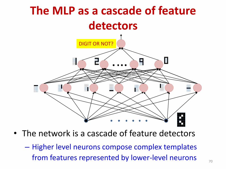
The MLP as a cascade of feature detectors
• The network is a cascade of feature detectors
– Higher level neurons compose complex templates
from features represented by lower-level neurons70
DIGIT OR NOT?
Story so far• Multi-layer perceptrons are connectionist computational models
• MLPs are Boolean machines
– They can model Boolean functions
– They can represent arbitrary decision boundaries over real inputs
• Perceptrons are correlation filters
– They detect patterns in the input
• MLPs are Boolean formulae over patterns detected by perceptrons
– Higher-level perceptrons may also be viewed as feature detectors
• Extra: MLP in classification
– The network will fire if the combination of the detected basic features matches an “acceptable” pattern for a desired class of signal
• E.g. Appropriate combinations of (Nose, Eyes, Eyebrows, Cheek, Chin) Face71

MLP as a continuous-valued regression
• A simple 3-unit MLP with a “summing” output unit can generate a “square pulse” over an input
– Output is 1 only if the input lies between T1 and T2
– T1 and T2 can be arbitrarily specified72
+x
1T1
T2
1
T1
T2
1
-1T1 T2 x
f(x)
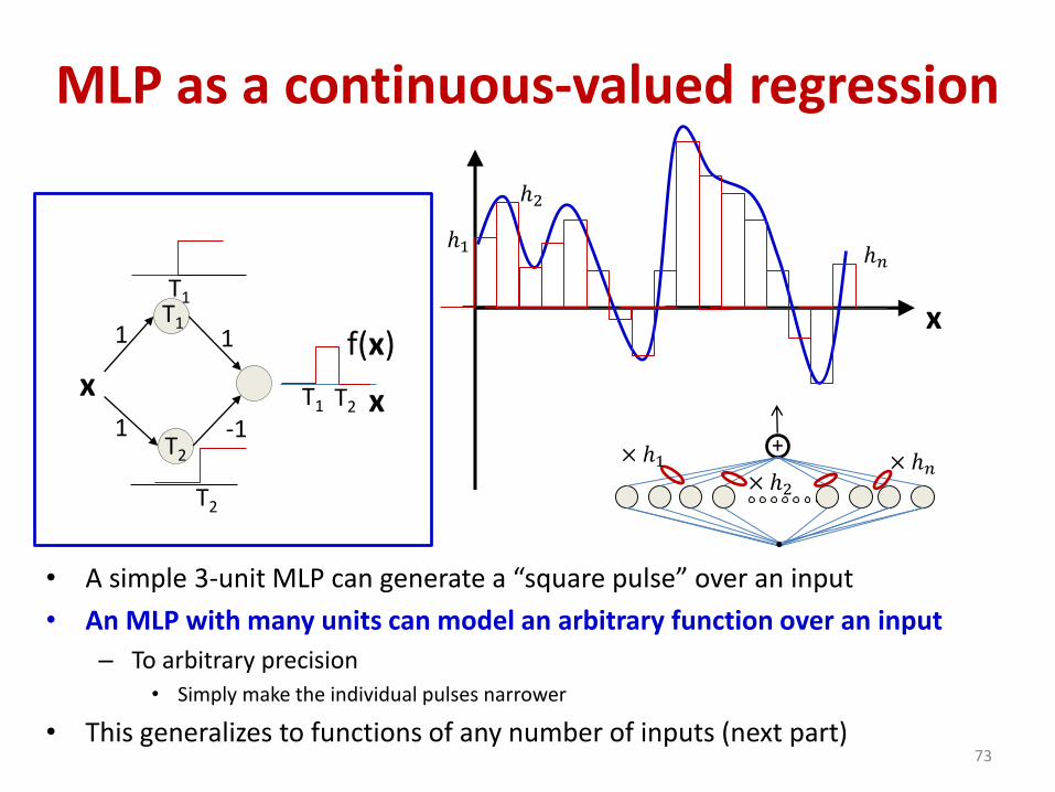
MLP as a continuous-valued regression
• A simple 3-unit MLP can generate a “square pulse” over an input
• An MLP with many units can model an arbitrary function over an input
– To arbitrary precision• Simply make the individual pulses narrower
• This generalizes to functions of any number of inputs (next part)73
x
1T1
T2
1
T1
T2
1
-1T1 T2 x
f(x)x
+× ℎ1× ℎ2
× ℎ𝑛
ℎ1
ℎ2
ℎ𝑛
Story so far
• Multi-layer perceptrons are connectionist
computational models
• MLPs are classification engines
– They can identify classes in the data
– Individual perceptrons are feature detectors
– The network will fire if the combination of the
detected basic features matches an “acceptable”
pattern for a desired class of signal
• MLP can also model continuous valued functions74
Neural Networks: Part 2: What can a network
represent
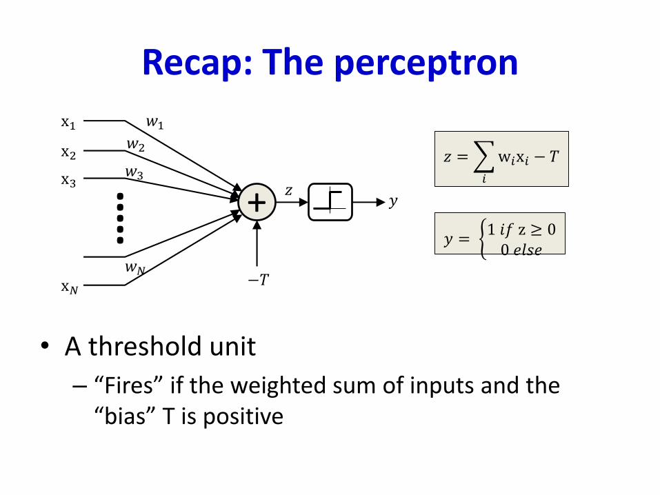
Recap: The perceptron
• A threshold unit
– “Fires” if the weighted sum of inputs and the “bias” T is positive
𝑦 = ቊ1 𝑖𝑓 z ≥ 00 𝑒𝑙𝑠𝑒
+.....
x1
x2
x3
x𝑁−𝑇
𝑧𝑦
𝑧 =
𝑖
w𝑖x𝑖 − 𝑇
𝑤1𝑤2
𝑤3
𝑤𝑁
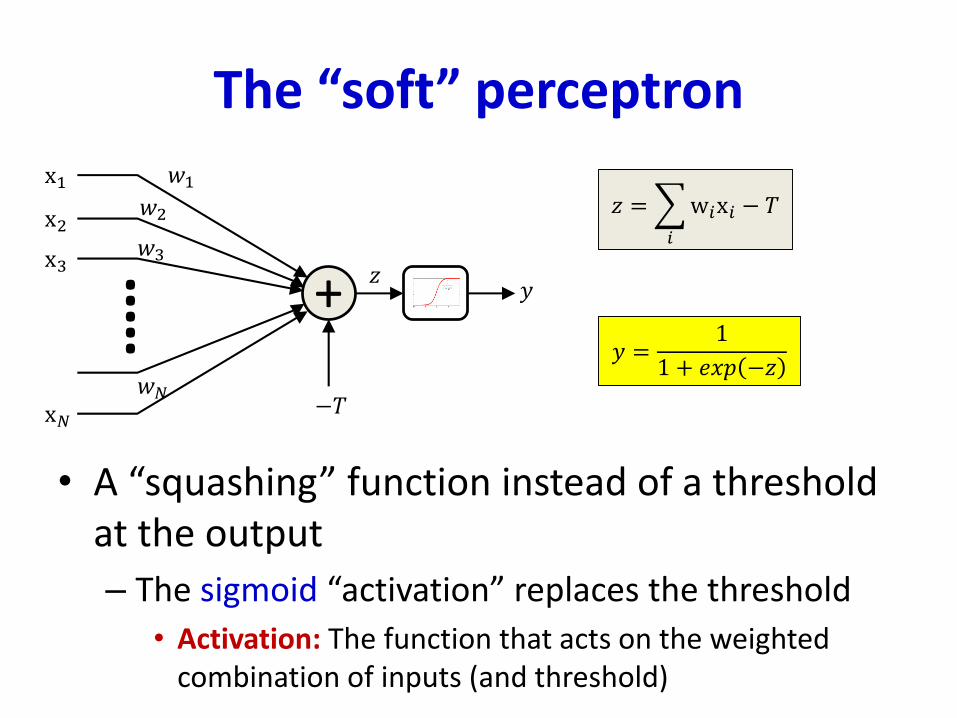
The “soft” perceptron
• A “squashing” function instead of a threshold at the output
– The sigmoid “activation” replaces the threshold
• Activation: The function that acts on the weighted combination of inputs (and threshold)
𝑦 =1
1 + 𝑒𝑥𝑝 −𝑧
+.....
x1
x2
x3
x𝑁−𝑇
𝑧𝑦
𝑤1𝑤2
𝑤3
𝑤𝑁
𝑧 =
𝑖
w𝑖x𝑖 − 𝑇
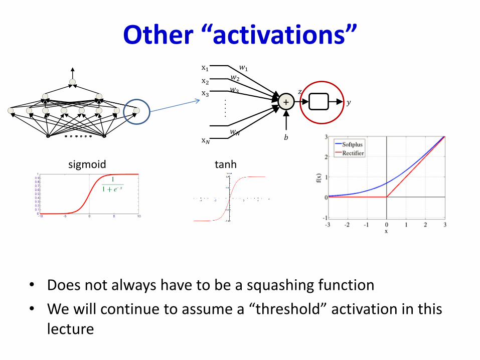
Other “activations”
• Does not always have to be a squashing function
• We will continue to assume a “threshold” activation in this lecture
sigmoid tanh
+.....
x1
x2
x3
x𝑁𝑏
𝑧
𝑦
𝑤1𝑤2
𝑤3
𝑤𝑁
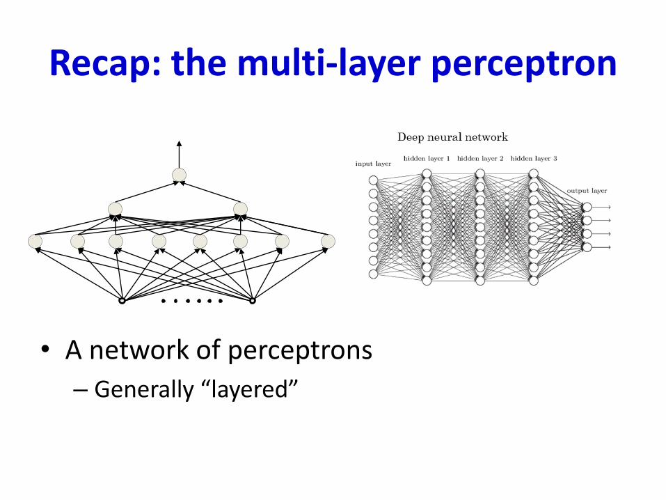
Recap: the multi-layer perceptron
• A network of perceptrons
– Generally “layered”
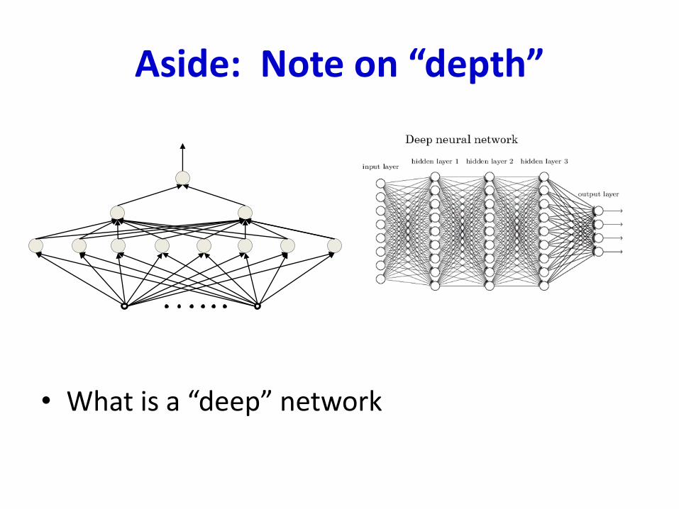
Aside: Note on “depth”
• What is a “deep” network
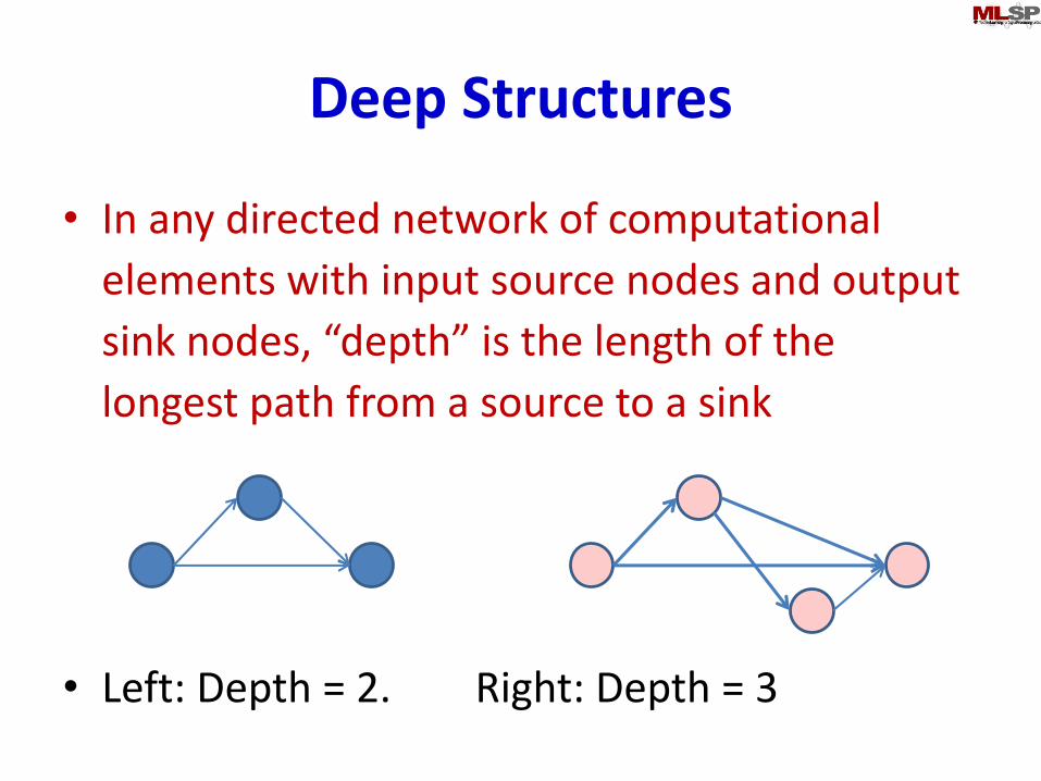
Deep Structures
• In any directed network of computational
elements with input source nodes and output
sink nodes, “depth” is the length of the
longest path from a source to a sink
• Left: Depth = 2. Right: Depth = 3
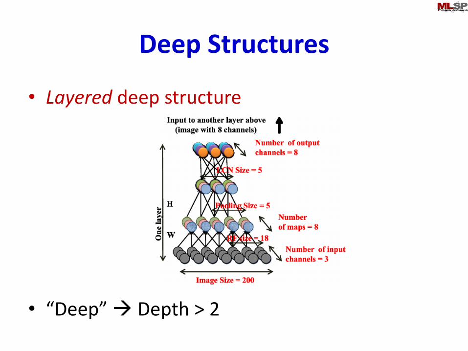
Deep Structures
• Layered deep structure
• “Deep” Depth > 2
The multi-layer perceptron
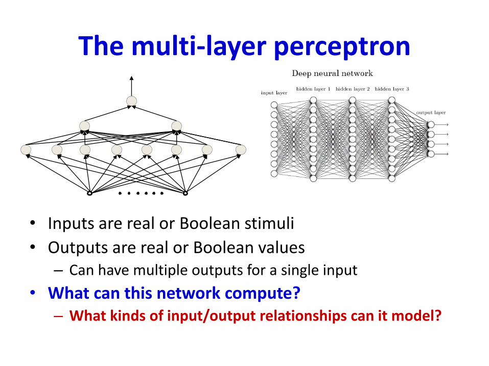
• Inputs are real or Boolean stimuli
• Outputs are real or Boolean values– Can have multiple outputs for a single input
• What can this network compute?– What kinds of input/output relationships can it model?
MLPs approximate functions
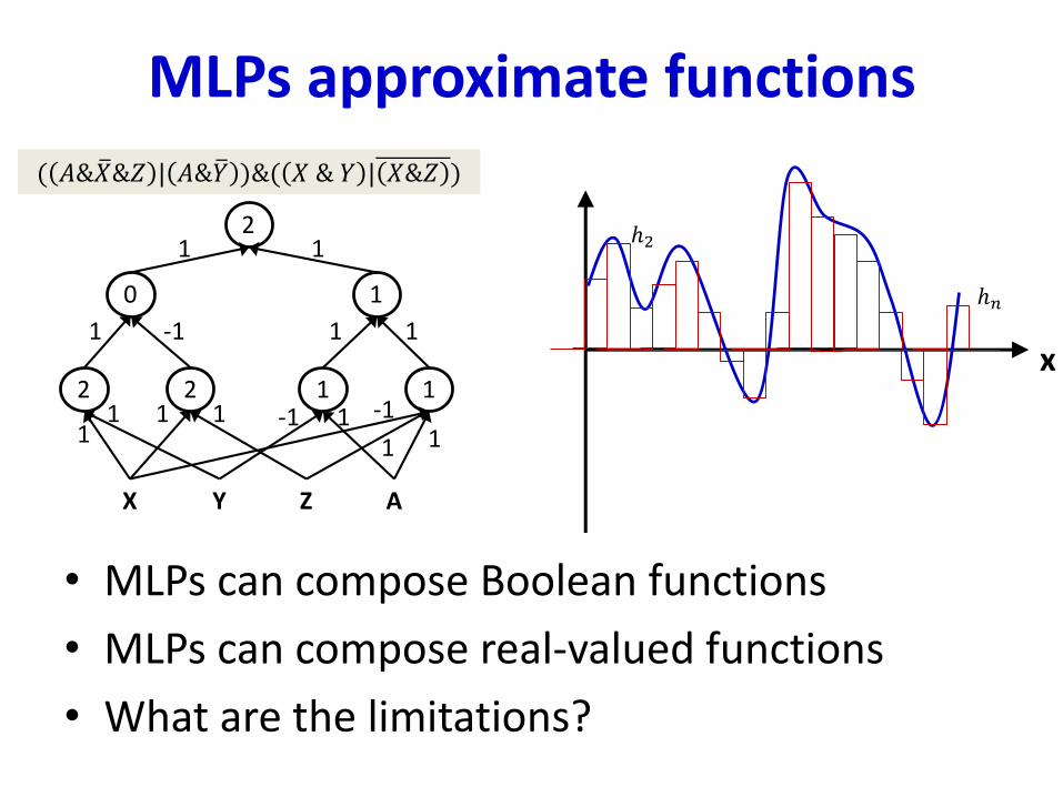
• MLPs can compose Boolean functions
• MLPs can compose real-valued functions
• What are the limitations?
( 𝐴& ത𝑋&𝑍 | 𝐴&ത𝑌 )&( 𝑋 & 𝑌 | 𝑋&𝑍 )
12 1 1 12 1 1
X Y Z A
10 11
12
11 1-111 -1
1 1
1 -1 1 1
11
x
ℎ2
ℎ𝑛
The MLP as a Boolean function
• How well do MLPs model Boolean functions?
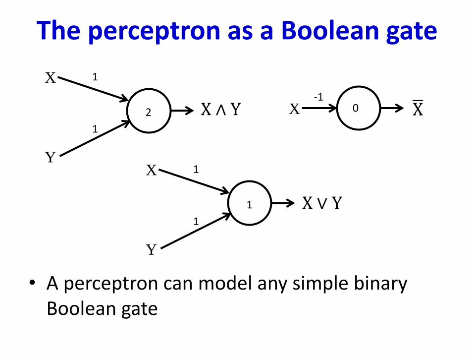
The perceptron as a Boolean gate
• A perceptron can model any simple binary Boolean gate
X
Y
1
1
2
X
Y
1
1
1
0X-1
X ∧ Y
X ∨ Y
ഥX
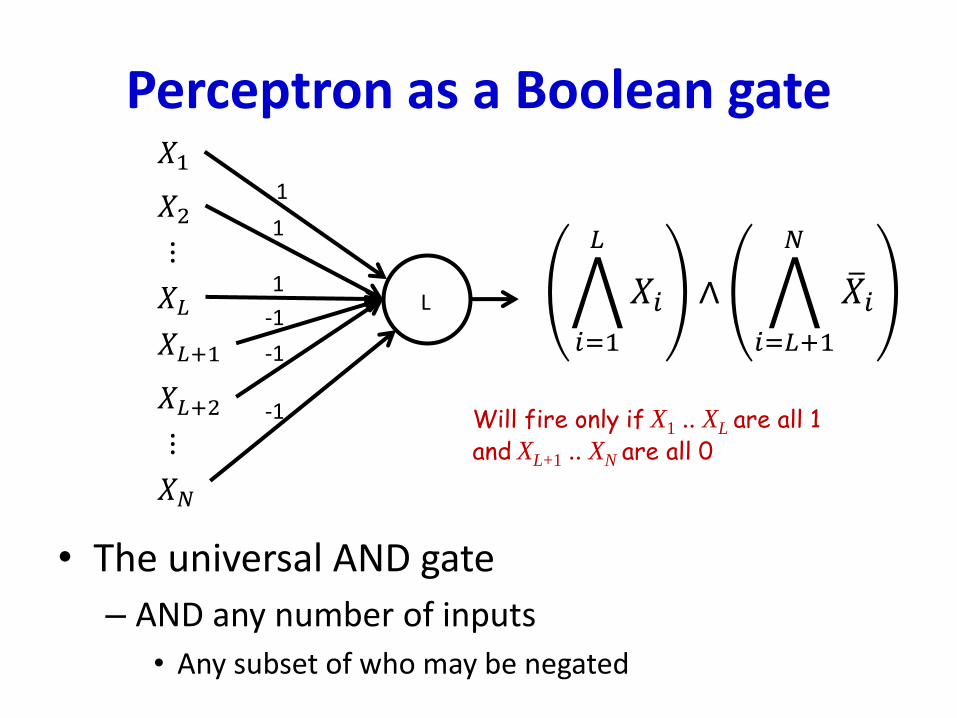
Perceptron as a Boolean gate
• The universal AND gate
– AND any number of inputs
• Any subset of who may be negated
𝑋11
1
L ሥ
𝑖=1
𝐿
𝑋𝑖 ∧ ሥ
𝑖=𝐿+1
𝑁
ത𝑋𝑖
𝑋2
𝑋𝐿
⋮
𝑋𝐿+1
𝑋𝐿+2
𝑋𝑁
⋮
1
-1
-1
-1 Will fire only if X1 .. XL are all 1and XL+1 .. XN are all 0
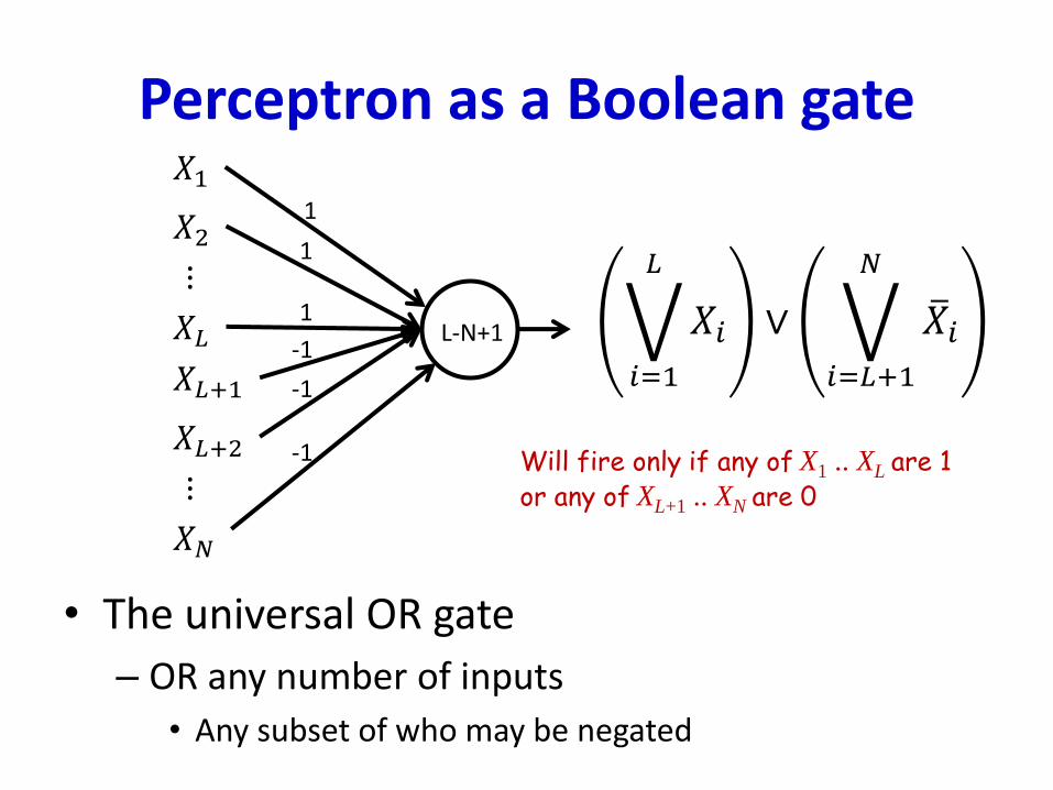
Perceptron as a Boolean gate
• The universal OR gate
– OR any number of inputs
• Any subset of who may be negated
𝑋11
1
L-N+1 ሧ
𝑖=1
𝐿
𝑋𝑖 ∨ ሧ
𝑖=𝐿+1
𝑁
ത𝑋𝑖
𝑋2
𝑋𝐿
⋮
𝑋𝐿+1
𝑋𝐿+2
𝑋𝑁
⋮
1
-1
-1
-1 Will fire only if any of X1 .. XL are 1or any of XL+1 .. XN are 0
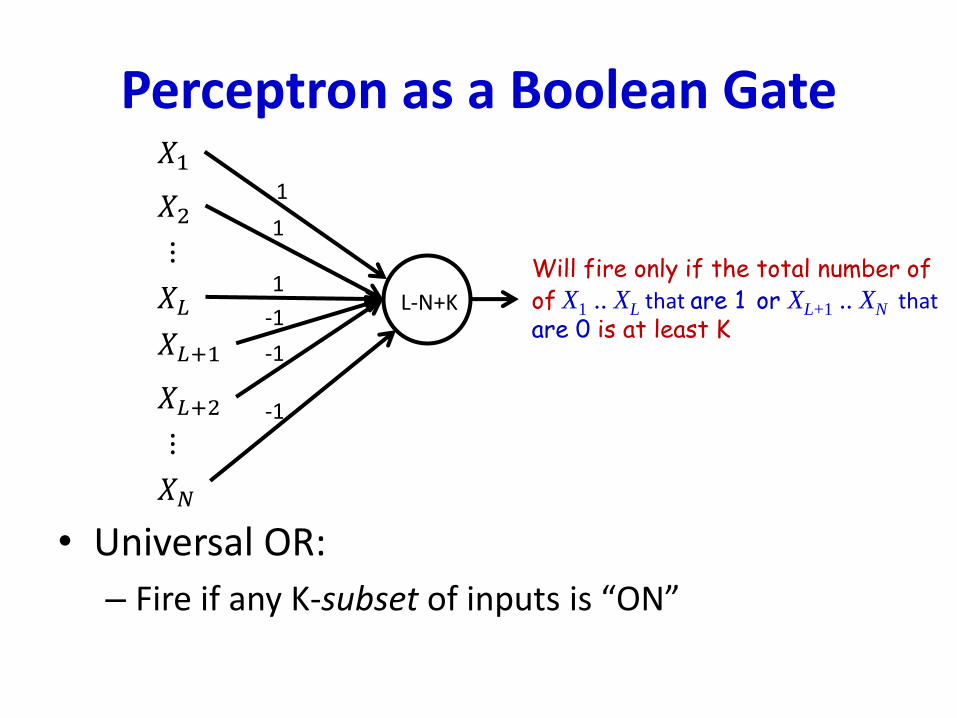
Perceptron as a Boolean Gate
• Universal OR:
– Fire if any K-subset of inputs is “ON”
𝑋11
1
L-N+K
𝑋2
𝑋𝐿
⋮
𝑋𝐿+1
𝑋𝐿+2
𝑋𝑁
⋮
1
-1
-1
-1
Will fire only if the total number ofof X1 .. XL that are 1 or XL+1 .. XN thatare 0 is at least K
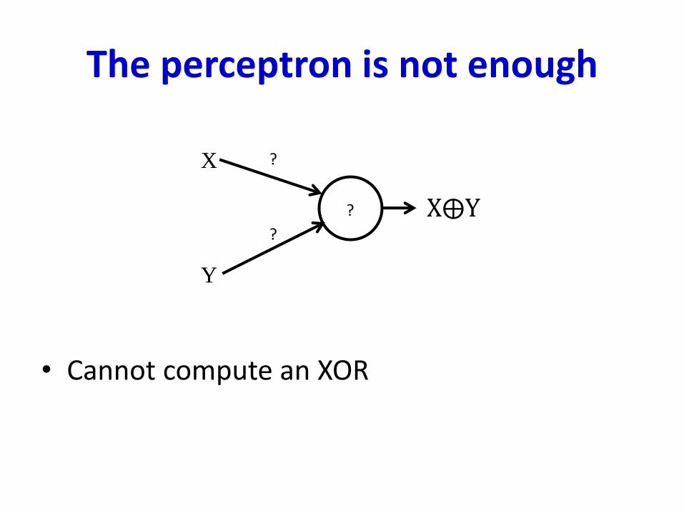
The perceptron is not enough
• Cannot compute an XOR
X
Y
?
?
? X⨁Y
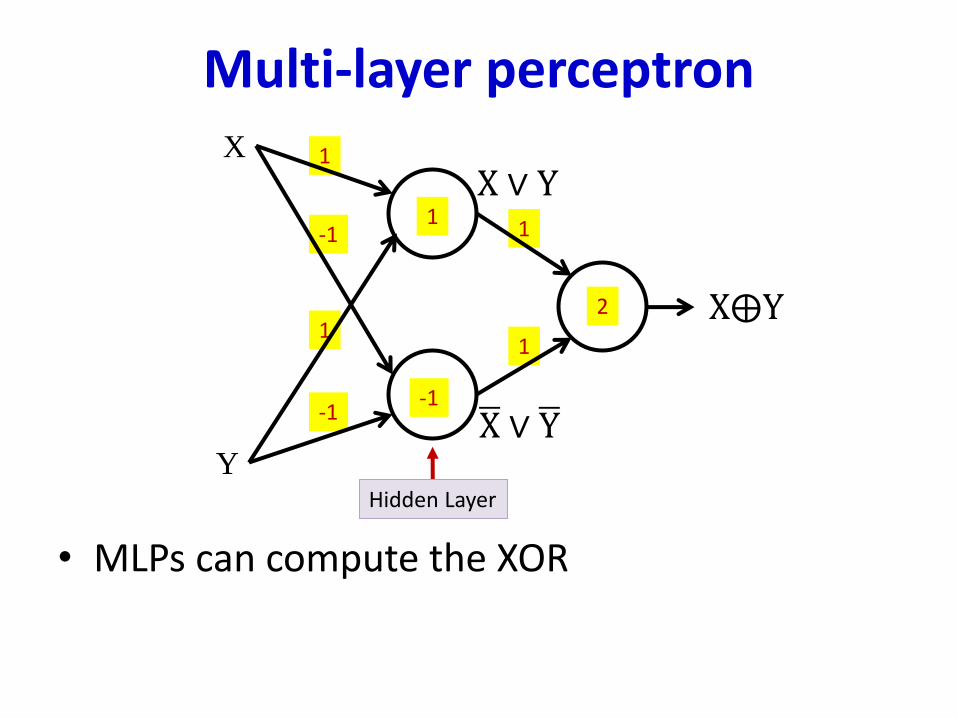
Multi-layer perceptron
• MLPs can compute the XOR
1
1
1
-1
1
-1
X
Y
1
X⨁Y
-1
2
X ∨ Y
ഥX ∨ ഥY
Hidden Layer
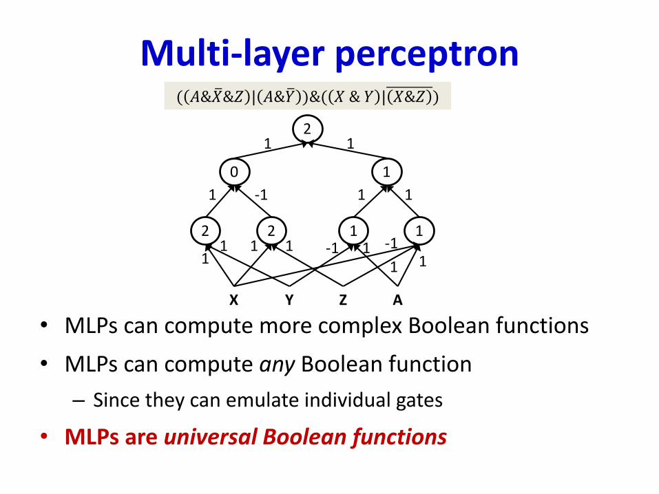
Multi-layer perceptron
• MLPs can compute more complex Boolean functions
• MLPs can compute any Boolean function
– Since they can emulate individual gates
• MLPs are universal Boolean functions
( 𝐴& ത𝑋&𝑍 | 𝐴&ത𝑌 )&( 𝑋 & 𝑌 | 𝑋&𝑍 )
12 1 1 12 1 1
X Y Z A
10 11
12
11 1-111 -1
1 1
1 -1 1 1
11
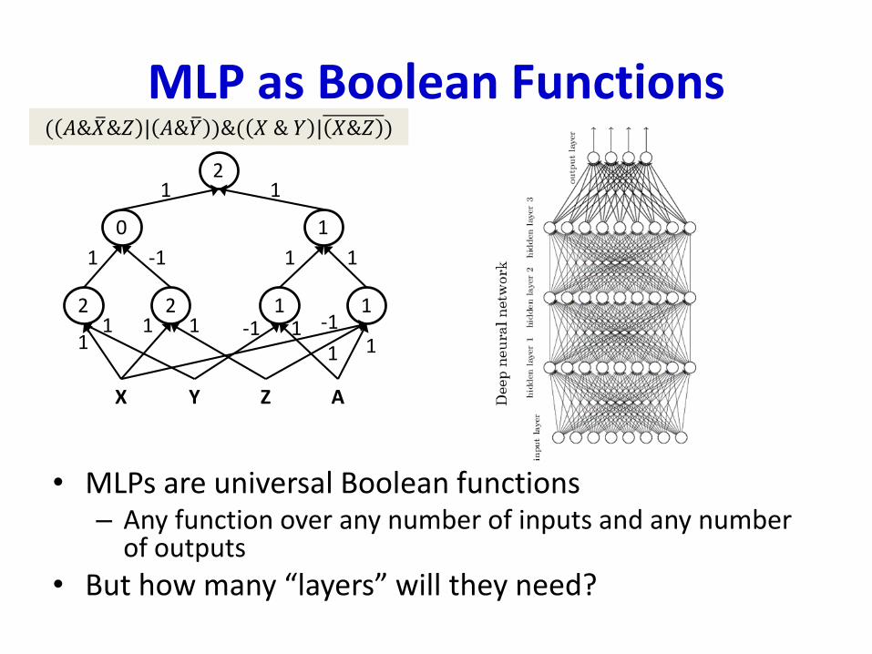
MLP as Boolean Functions
• MLPs are universal Boolean functions– Any function over any number of inputs and any number
of outputs
• But how many “layers” will they need?
( 𝐴& ത𝑋&𝑍 | 𝐴&ത𝑌 )&( 𝑋 & 𝑌 | 𝑋&𝑍 )
12 1 1 12 1 1
X Y Z A
10 11
12
11 1-111 -1
1 1
1 -1 1 1
11
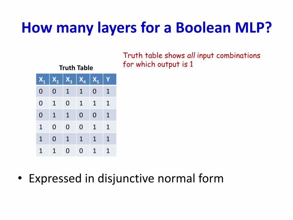
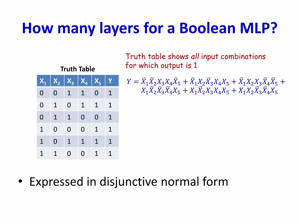
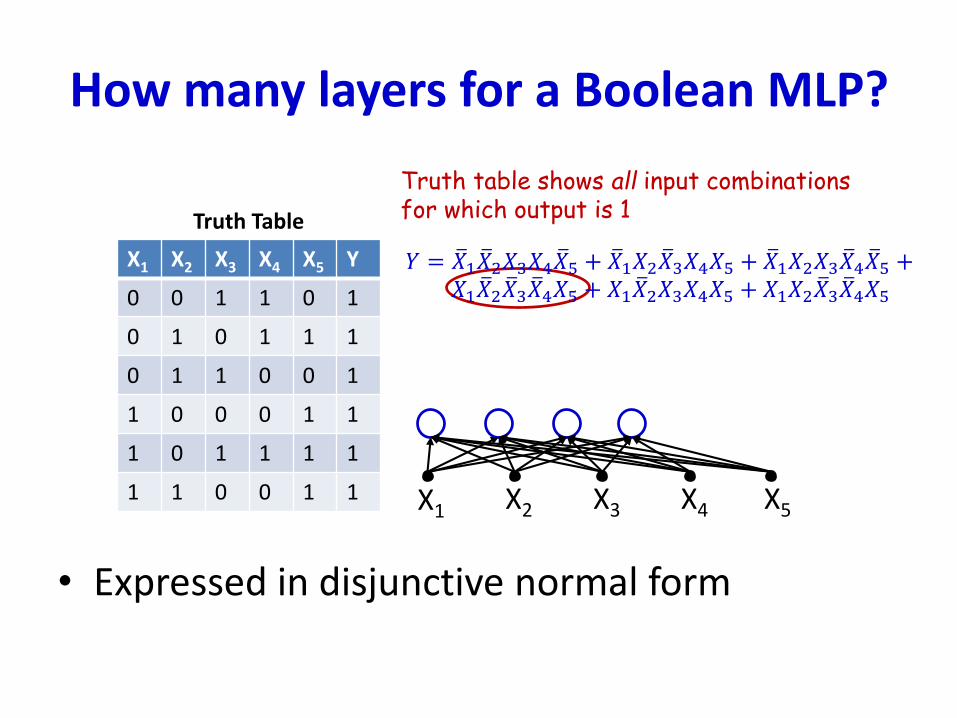
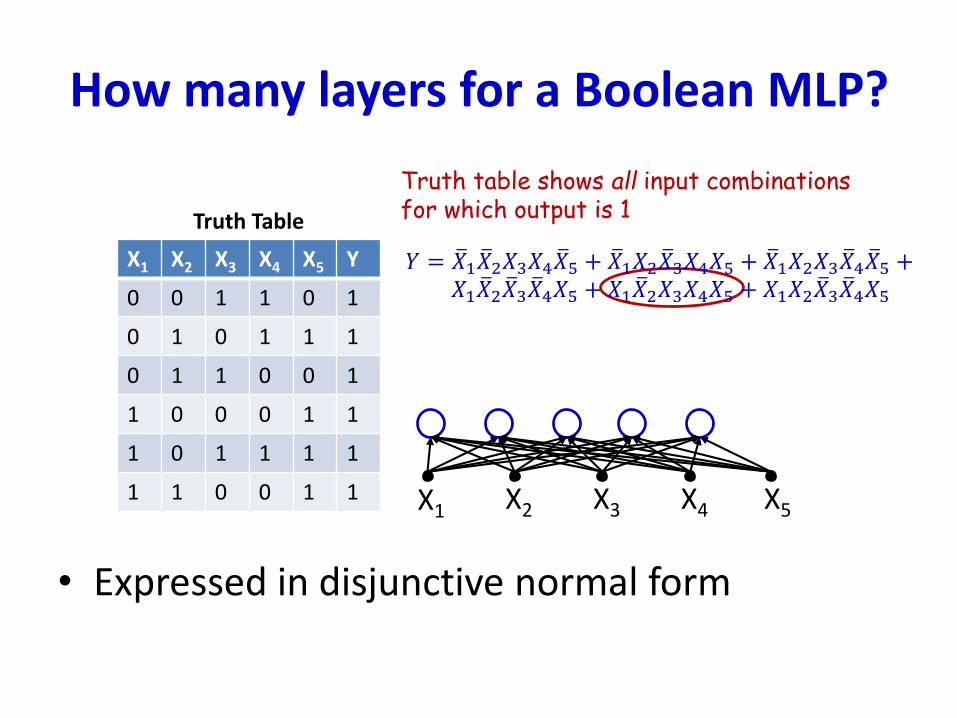
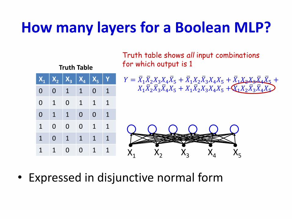
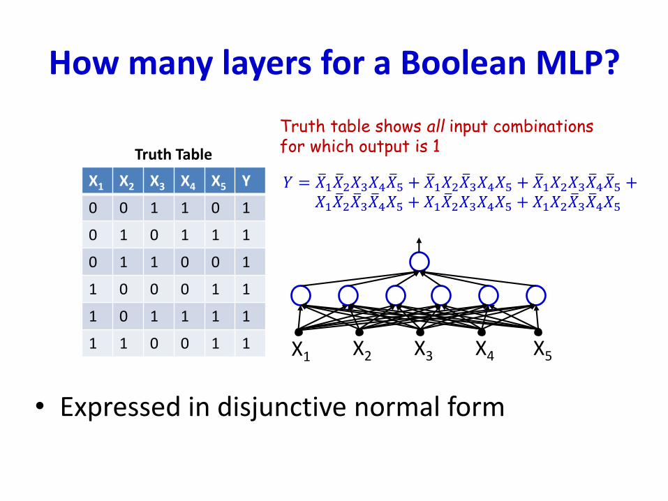
How many layers for a Boolean MLP?
• Expressed in disjunctive normal form
X1 X2 X3 X4 X5 Y
0 0 1 1 0 1
0 1 0 1 1 1
0 1 1 0 0 1
1 0 0 0 1 1
1 0 1 1 1 1
1 1 0 0 1 1
Truth Table
Truth table shows all input combinationsfor which output is 1
How many layers for a Boolean MLP?
• Expressed in disjunctive normal form
X1 X2 X3 X4 X5 Y
0 0 1 1 0 1
0 1 0 1 1 1
0 1 1 0 0 1
1 0 0 0 1 1
1 0 1 1 1 1
1 1 0 0 1 1
Truth Table
𝑌 = ത𝑋1 ത𝑋2𝑋3𝑋4 ത𝑋5 + ത𝑋1𝑋2 ത𝑋3𝑋4𝑋5 + ത𝑋1𝑋2𝑋3 ത𝑋4 ത𝑋5 +𝑋1 ത𝑋2 ത𝑋3 ത𝑋4𝑋5 + 𝑋1 ത𝑋2𝑋3𝑋4𝑋5 + 𝑋1𝑋2 ത𝑋3 ത𝑋4𝑋5
Truth table shows all input combinationsfor which output is 1
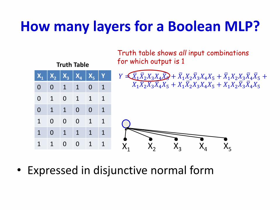
How many layers for a Boolean MLP?
• Expressed in disjunctive normal form
X1 X2 X3 X4 X5 Y
0 0 1 1 0 1
0 1 0 1 1 1
0 1 1 0 0 1
1 0 0 0 1 1
1 0 1 1 1 1
1 1 0 0 1 1
Truth Table
Truth table shows all input combinationsfor which output is 1
X1 X2 X3 X4 X5
𝑌 = ത𝑋1 ത𝑋2𝑋3𝑋4 ത𝑋5 + ത𝑋1𝑋2 ത𝑋3𝑋4𝑋5 + ത𝑋1𝑋2𝑋3 ത𝑋4 ത𝑋5 +𝑋1 ത𝑋2 ത𝑋3 ത𝑋4𝑋5 + 𝑋1 ത𝑋2𝑋3𝑋4𝑋5 + 𝑋1𝑋2 ത𝑋3 ത𝑋4𝑋5
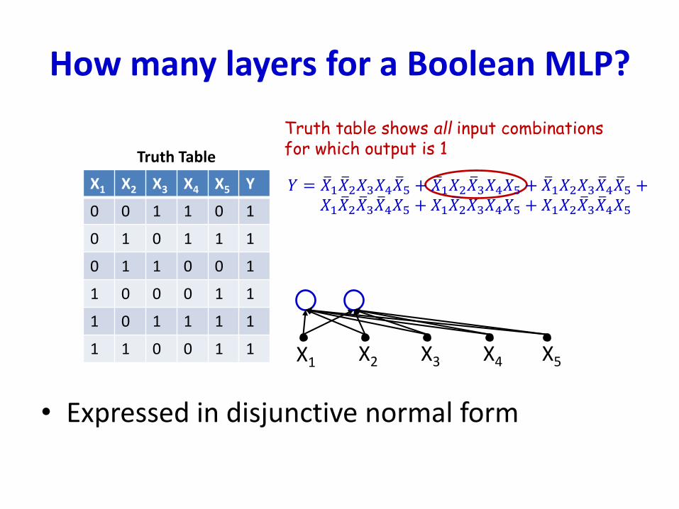
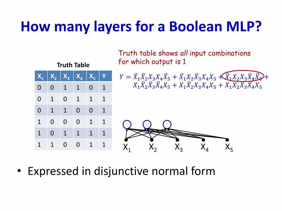
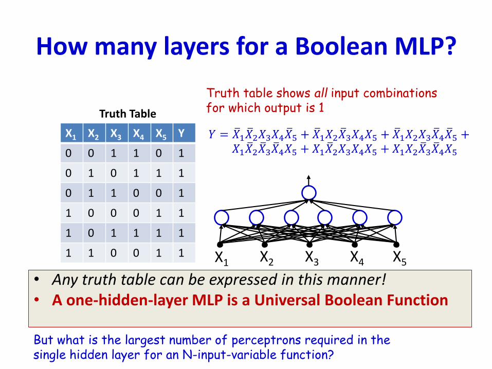
How many layers for a Boolean MLP?
• Any truth table can be expressed in this manner!• A one-hidden-layer MLP is a Universal Boolean Function
X1 X2 X3 X4 X5 Y
0 0 1 1 0 1
0 1 0 1 1 1
0 1 1 0 0 1
1 0 0 0 1 1
1 0 1 1 1 1
1 1 0 0 1 1
Truth Table
Truth table shows all input combinationsfor which output is 1
X1 X2 X3 X4 X5
But what is the largest number of perceptrons required in the single hidden layer for an N-input-variable function?
𝑌 = ത𝑋1 ത𝑋2𝑋3𝑋4 ത𝑋5 + ത𝑋1𝑋2 ത𝑋3𝑋4𝑋5 + ത𝑋1𝑋2𝑋3 ത𝑋4 ത𝑋5 +𝑋1 ത𝑋2 ത𝑋3 ത𝑋4𝑋5 + 𝑋1 ത𝑋2𝑋3𝑋4𝑋5 + 𝑋1𝑋2 ത𝑋3 ത𝑋4𝑋5
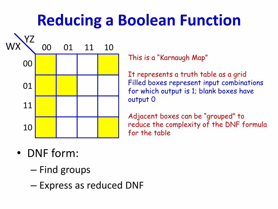
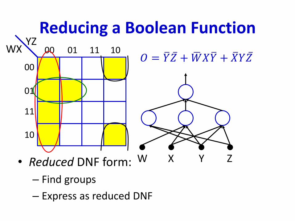
Reducing a Boolean Function
• DNF form:
– Find groups
– Express as reduced DNF
This is a “Karnaugh Map”
It represents a truth table as a gridFilled boxes represent input combinationsfor which output is 1; blank boxes haveoutput 0
Adjacent boxes can be “grouped” to reduce the complexity of the DNF formula for the table
00 01 11 10
00
01
11
10
YZWX
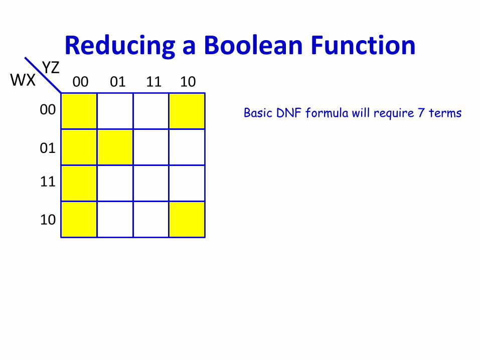
Reducing a Boolean Function00 01 11 10
00
01
11
10
YZWX
Basic DNF formula will require 7 terms
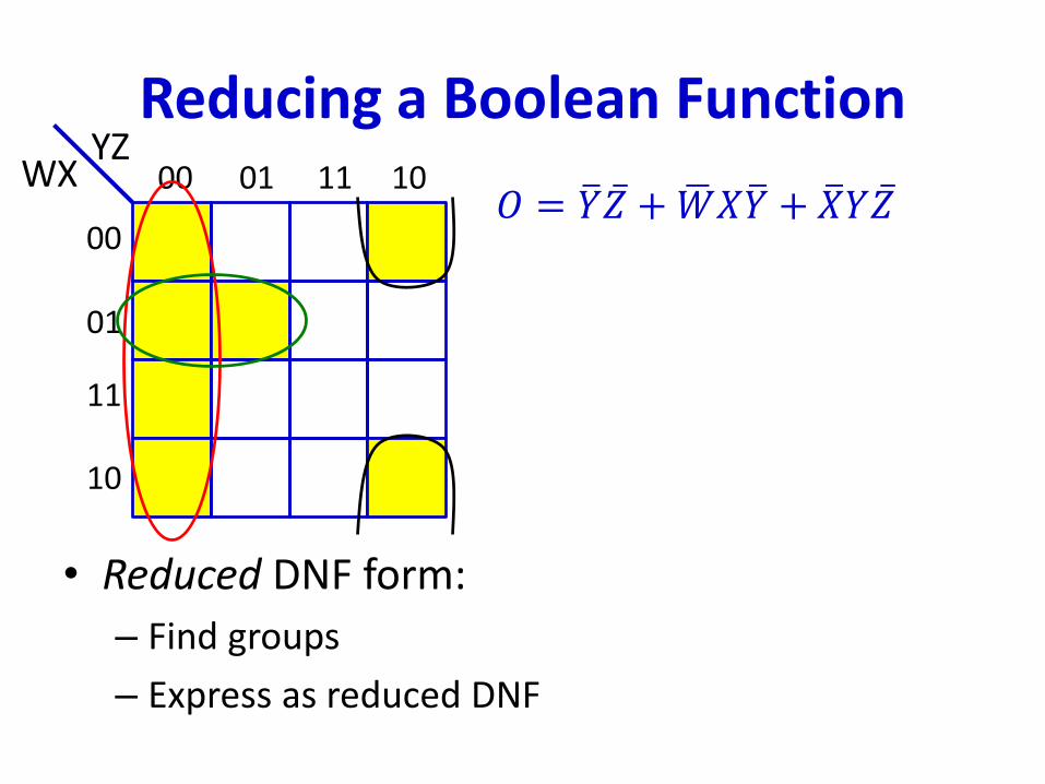
Reducing a Boolean Function
• Reduced DNF form:
– Find groups
– Express as reduced DNF
𝑂 = ത𝑌 ҧ𝑍 + ഥ𝑊𝑋ത𝑌 + ത𝑋𝑌 ҧ𝑍00 01 11 10
00
01
11
10
YZWX
Reducing a Boolean Function
• Reduced DNF form:
– Find groups
– Express as reduced DNF
𝑂 = ത𝑌 ҧ𝑍 + ഥ𝑊𝑋ത𝑌 + ത𝑋𝑌 ҧ𝑍00 01 11 10
00
01
11
10
YZWX
W X Y Z
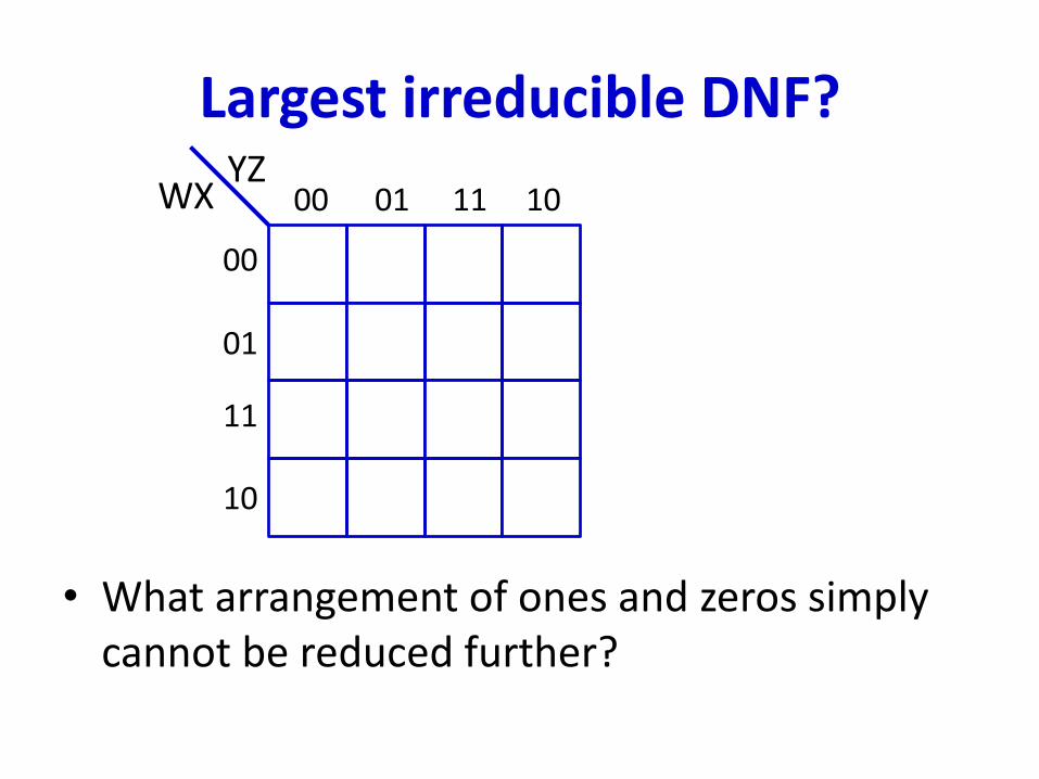
Largest irreducible DNF?
• What arrangement of ones and zeros simply cannot be reduced further?
00 01 11 10
00
01
11
10
YZWX
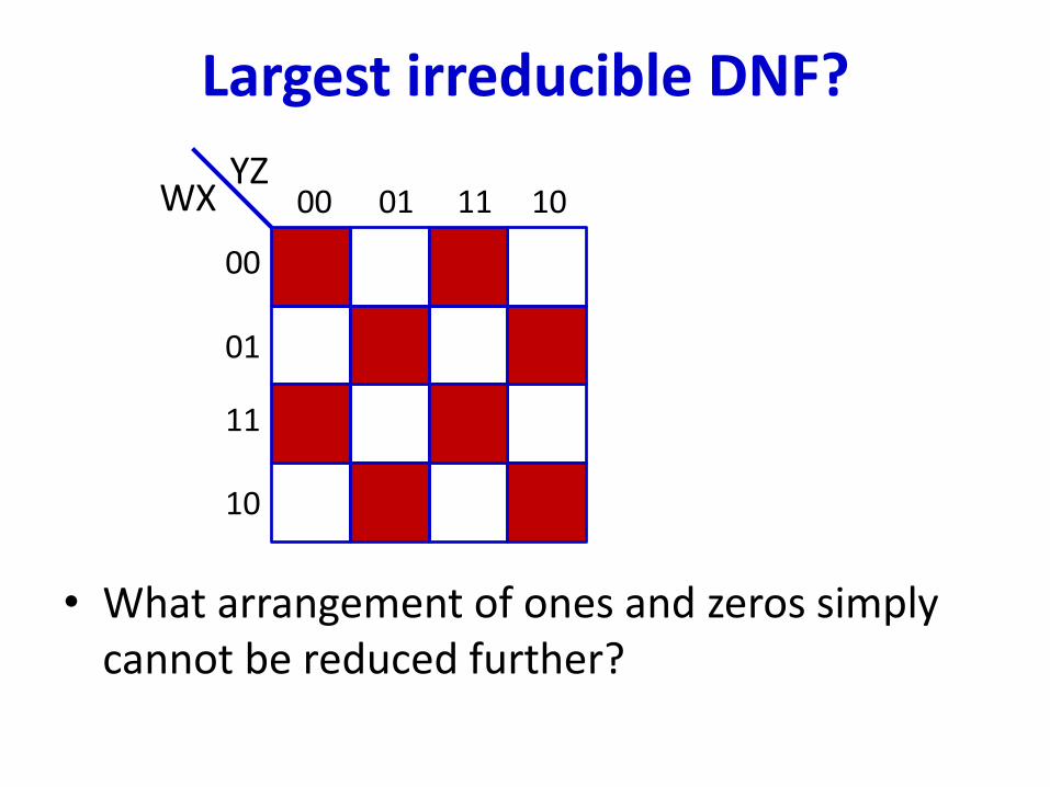
Largest irreducible DNF?
• What arrangement of ones and zeros simply cannot be reduced further?
00 01 11 10
00
01
11
10
YZWX
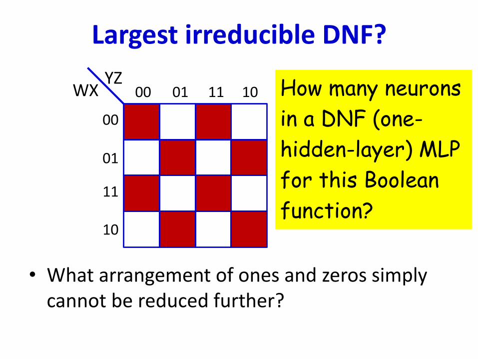
Largest irreducible DNF?
• What arrangement of ones and zeros simply cannot be reduced further?
00 01 11 10
00
01
11
10
YZWX How many neurons
in a DNF (one-
hidden-layer) MLP
for this Boolean
function?
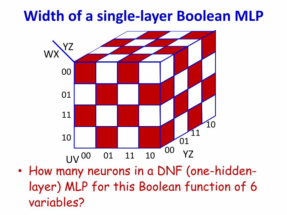
• How many neurons in a DNF (one-hidden-layer) MLP for this Boolean function of 6 variables?
00 01 11 10
00
01
11
10
YZWX
1011
0100 YZUV
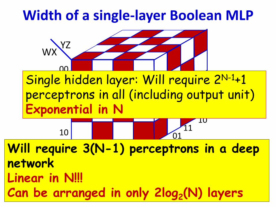
Width of a single-layer Boolean MLP
• How many neurons in a DNF (one-hidden-
layer) MLP for this Boolean function
00 01 11 10
00
01
11
10
YZWX
1011
0100 YZUV
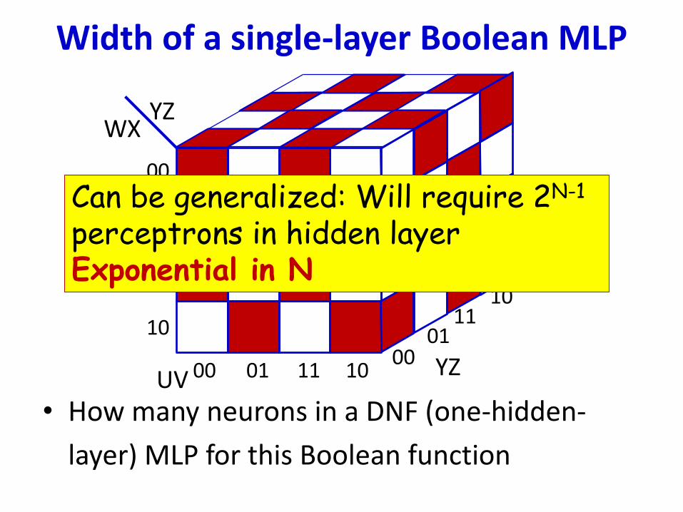
Width of a single-layer Boolean MLP
Can be generalized: Will require 2N-1
perceptrons in hidden layerExponential in N
• How many neurons in a DNF (one-hidden-
layer) MLP for this Boolean function
00 01 11 10
00
01
11
10
YZWX
1011
0100 YZUV
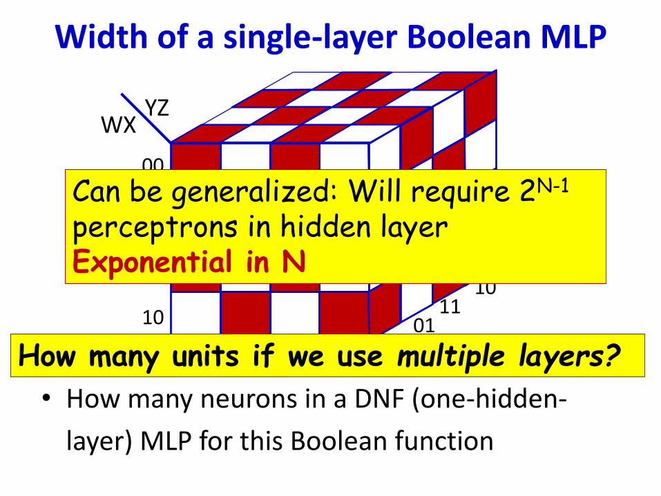
Width of a single-layer Boolean MLP
Can be generalized: Will require 2N-1
perceptrons in hidden layerExponential in N
How many units if we use multiple layers?
00 01 11 10
00
01
11
10
YZWX
1011
0100 YZ
UV
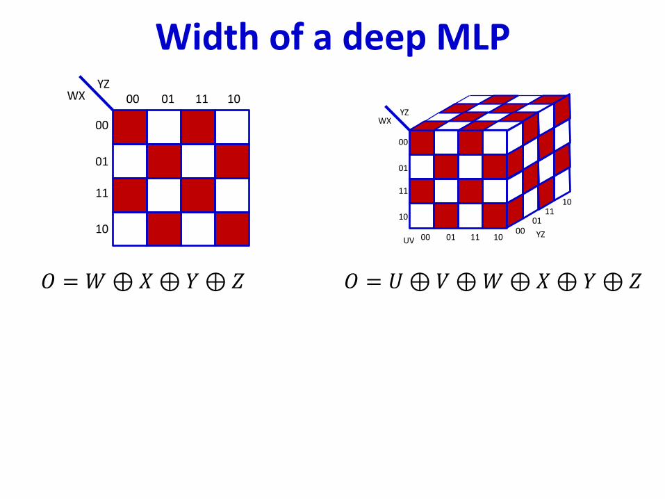
Width of a deep MLP
00 01 11 10
00
01
11
10
YZWX
𝑂 = 𝑊⊕𝑋⊕ 𝑌⊕ 𝑍 𝑂 = 𝑈⊕ 𝑉⊕𝑊⊕𝑋⊕𝑌⊕ 𝑍
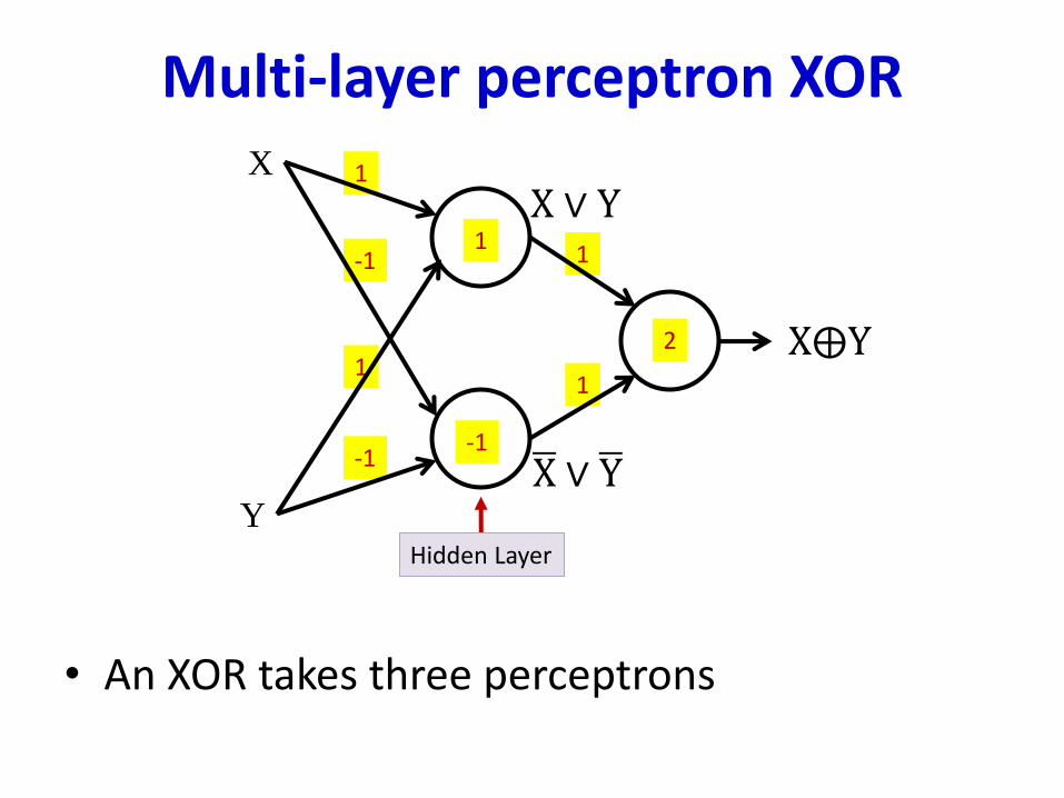
Multi-layer perceptron XOR
• An XOR takes three perceptrons
1
1
1
-1
1
-1
X
Y
1
X⨁Y
-1
2
X ∨ Y
ഥX ∨ ഥY
Hidden Layer
• An XOR needs 3 perceptrons
• This network will require 3x3 = 9 perceptrons
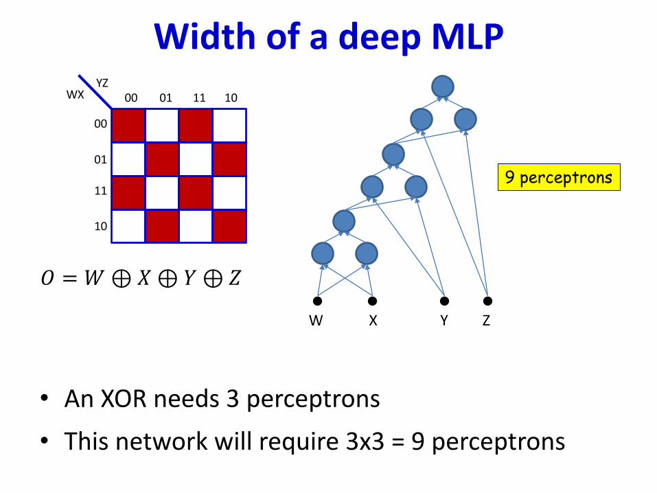
Width of a deep MLP
00 01 11 10
00
01
11
10
YZWX
𝑂 = 𝑊⊕𝑋⊕ 𝑌⊕ 𝑍
W X Y Z
9 perceptrons
• An XOR needs 3 perceptrons
• This network will require 3x5 = 15 perceptrons
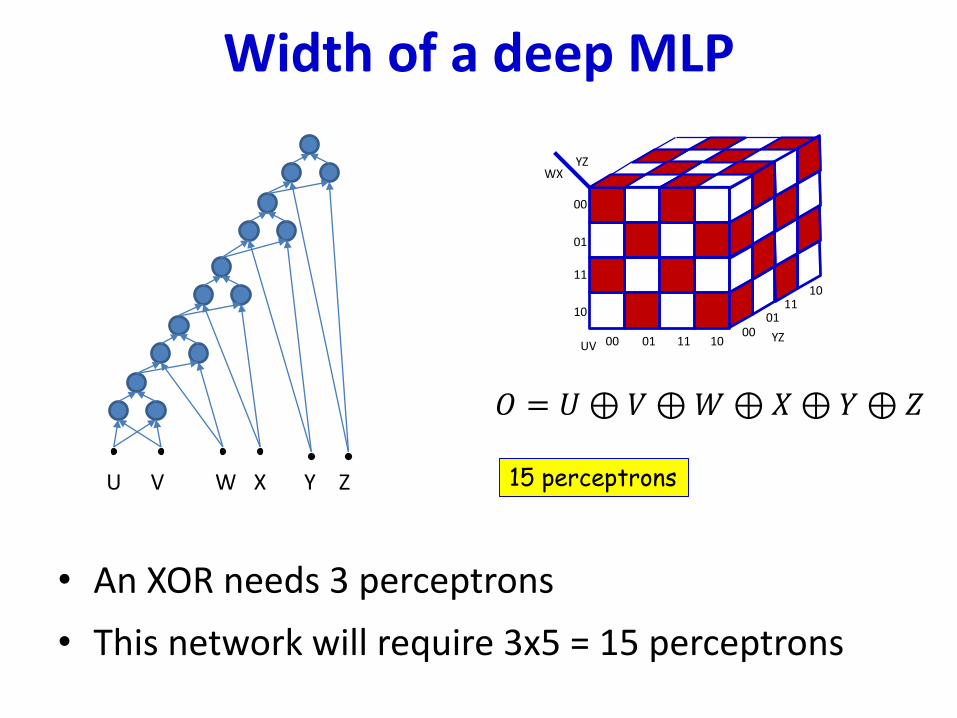
Width of a deep MLP
U V W X Y Z
00 01 11 10
00
01
11
10
YZWX
1011
0100 YZ
UV
𝑂 = 𝑈⊕ 𝑉⊕𝑊⊕𝑋⊕𝑌⊕ 𝑍
15 perceptrons
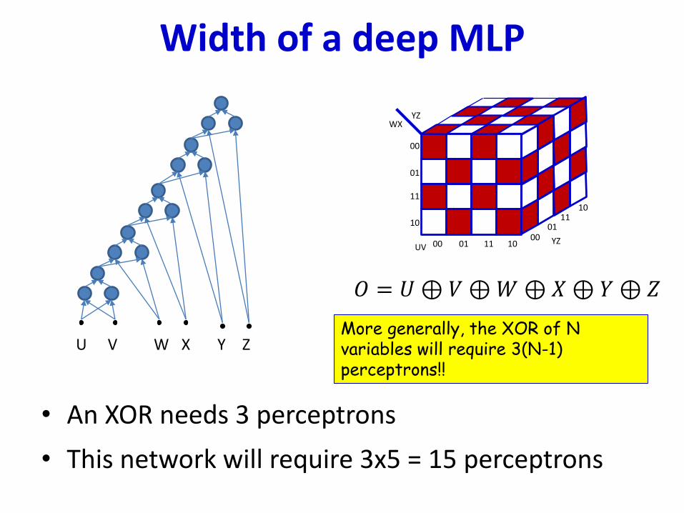
• An XOR needs 3 perceptrons
• This network will require 3x5 = 15 perceptrons
Width of a deep MLP
U V W X Y Z
00 01 11 10
00
01
11
10
YZWX
1011
0100 YZ
UV
𝑂 = 𝑈⊕ 𝑉⊕𝑊⊕𝑋⊕𝑌⊕ 𝑍
More generally, the XOR of N variables will require 3(N-1) perceptrons!!
• How many neurons in a DNF (one-hidden-
layer) MLP for this Boolean function
00 01 11 10
00
01
11
10
YZWX
1011
0100 YZUV
Width of a single-layer Boolean MLP
Single hidden layer: Will require 2N-1+1 perceptrons in all (including output unit)Exponential in N
Will require 3(N-1) perceptrons in a deep networkLinear in N!!!Can be arranged in only 2log2(N) layers
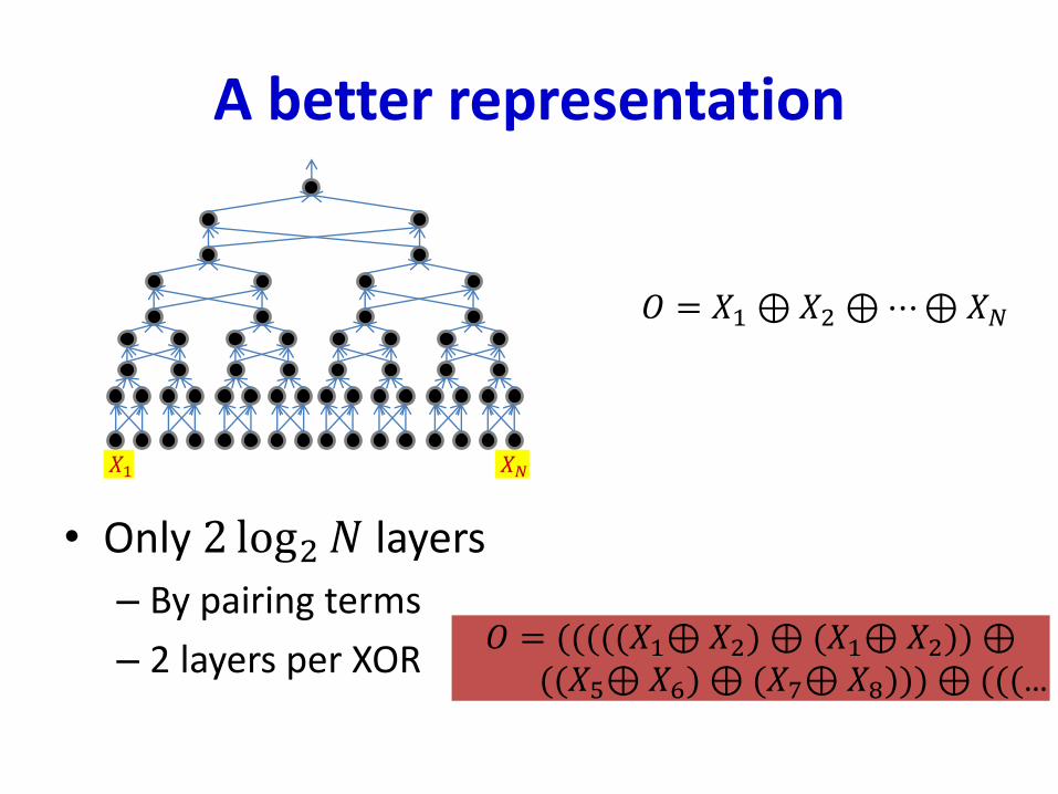
A better representation
• Only 2 log2𝑁 layers
– By pairing terms
– 2 layers per XOR
𝑂 = 𝑋1 ⊕𝑋2 ⊕⋯⊕𝑋𝑁
𝑋1 𝑋𝑁
𝑂 = (((((𝑋1⊕𝑋2) ⊕ (𝑋1⊕𝑋2)) ⊕((𝑋5⊕𝑋6) ⊕ (𝑋7⊕𝑋8))) ⊕ (((…
𝑍1 𝑍𝑀
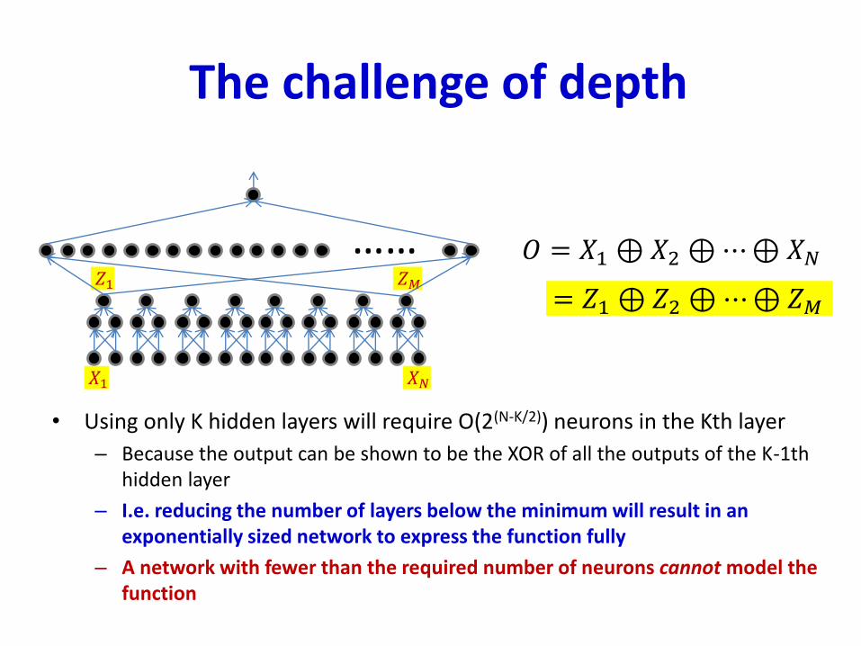
The challenge of depth
• Using only K hidden layers will require O(2(N-K/2)) neurons in the Kth layer
– Because the output can be shown to be the XOR of all the outputs of the K-1th hidden layer
– I.e. reducing the number of layers below the minimum will result in an exponentially sized network to express the function fully
– A network with fewer than the required number of neurons cannot model the function
𝑂 = 𝑋1 ⊕𝑋2 ⊕⋯⊕𝑋𝑁……= 𝑍1 ⊕𝑍2 ⊕⋯⊕𝑍𝑀
𝑋1 𝑋𝑁
Recap: The need for depth
• Deep Boolean MLPs that scale linearly with the number of inputs …
• … can become exponentially large if recast using only one layer
• It gets worse..
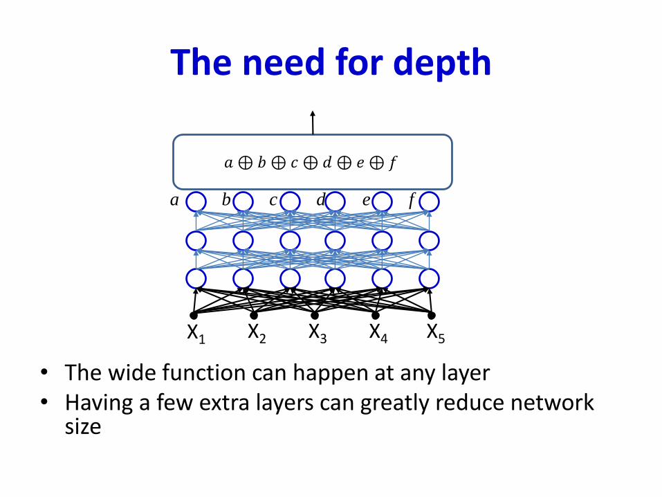
The need for depth
• The wide function can happen at any layer• Having a few extra layers can greatly reduce network
size
X1 X2 X3 X4 X5
a b c d e f
𝑎 ⊕ 𝑏⊕ 𝑐 ⊕ 𝑑⊕ 𝑒⊕ 𝑓
Network size: summary
• An MLP is a universal Boolean function
• But can represent a given function only if
– It is sufficiently wide
– It is sufficiently deep
– Depth can be traded off for (sometimes) exponential growth of the width of the network
• Optimal width and depth depend on the number of variables and the complexity of the Boolean function
– Complexity: minimal number of terms in DNF formula to represent it
Story so far
• Multi-layer perceptrons are Universal Boolean Machines
• Even a network with a single hidden layer is a universal Boolean machine
– But a single-layer network may require an exponentially large number of perceptrons
• Deeper networks may require far fewer neurons than shallower networks to express the same function
– Could be exponentially smaller
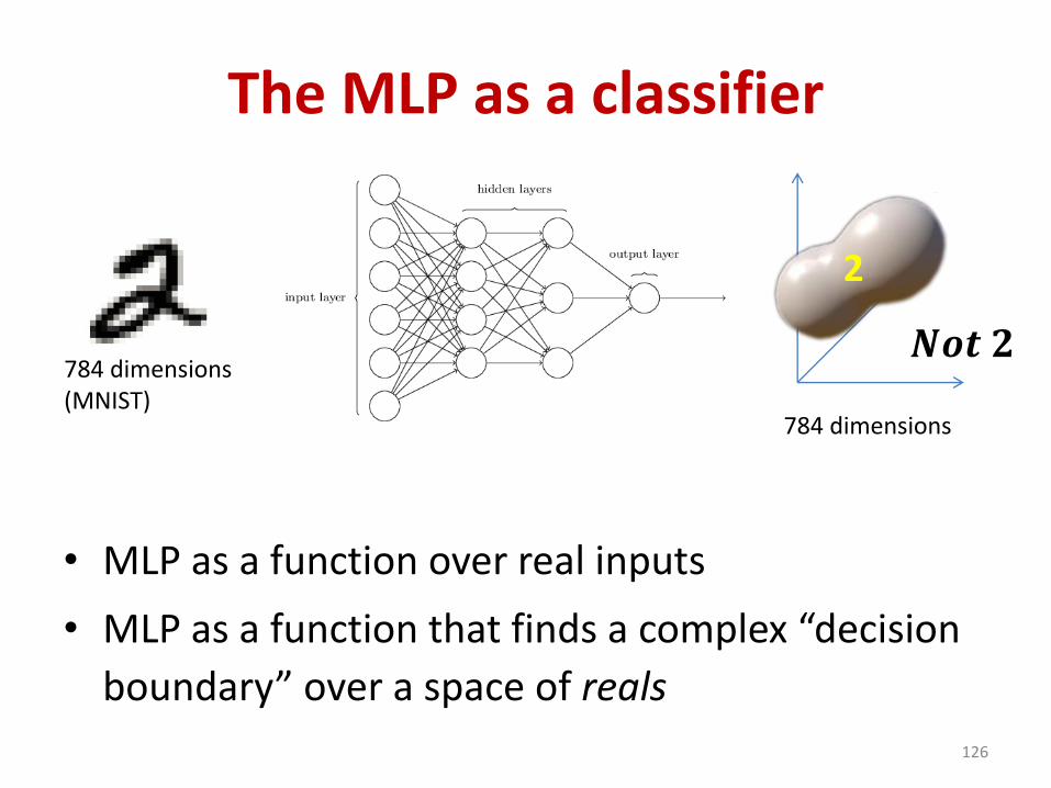
The MLP as a classifier
• MLP as a function over real inputs
• MLP as a function that finds a complex “decision
boundary” over a space of reals
126
784 dimensions(MNIST)
784 dimensions
2
𝑵𝒐𝒕 𝟐

A Perceptron on Reals
• A perceptron operates on real-valued vectors– This is a linear classifier 127
x1
x2w1x1+w2x2=T
𝑦 = ൞1 𝑖𝑓
𝑖
𝑤𝑖x𝑖 ≥ 𝑇
0 𝑒𝑙𝑠𝑒
x1
x2
1
0
x1
x2
x3
xN
Booleans over the reals
• The network must fire if the input is in the coloured area
128
x1
x2
x1
x2
AND
5
44
4
4
4
3
3
3
33 x1x2
𝑖=1
𝑁
y𝑖 ≥ 5?
y1 y5y2 y3 y4
More complex decision boundaries
• Network to fire if the input is in the yellow area
– “OR” two polygons
– A third layer is required129
x2
AND AND
OR
x1 x1 x2
Complex decision boundaries
• Can compose arbitrarily complex decision
boundaries
130
Complex decision boundaries
• Can compose arbitrarily complex decision
boundaries
131
AND
OR
x1 x2
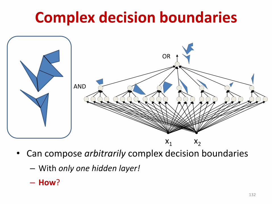
Complex decision boundaries
• Can compose arbitrarily complex decision boundaries
– With only one hidden layer!
– How?132
AND
OR
x1 x2
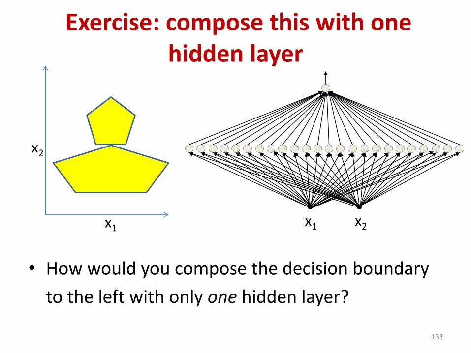
Exercise: compose this with one hidden layer
• How would you compose the decision boundary
to the left with only one hidden layer?
133
x1 x2
x2
x1
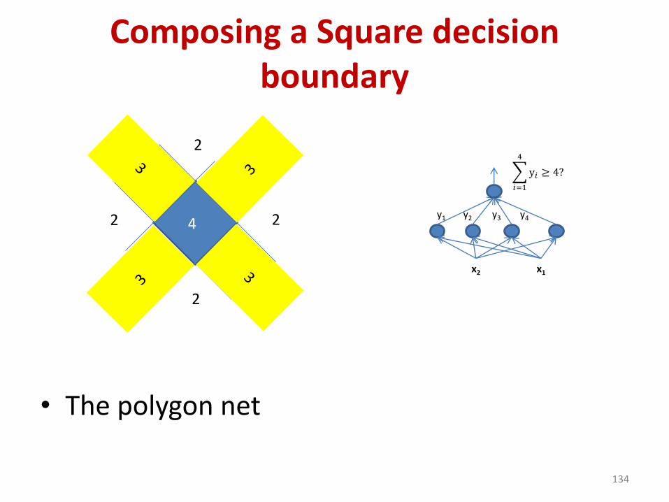
Composing a Square decision boundary
• The polygon net
134
4
x1x2
𝑖=1
4
y𝑖 ≥ 4?
y1 y2 y3 y4
2
2
2
2
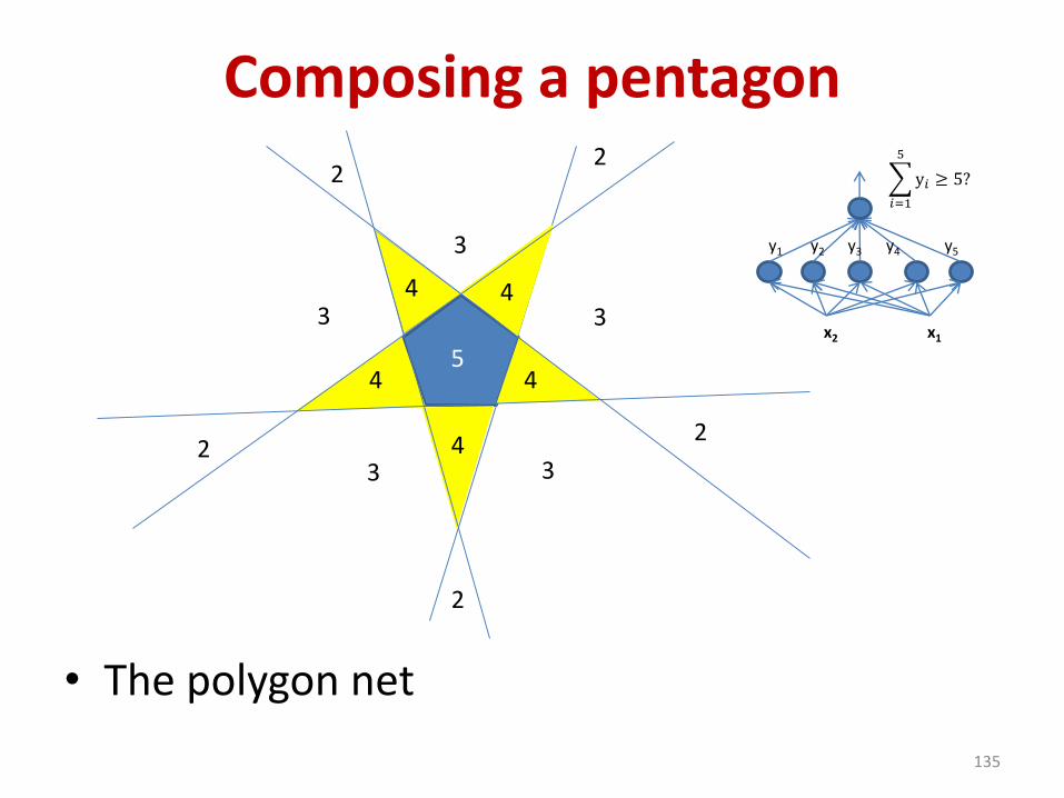
Composing a pentagon
• The polygon net
135
5
44
4
4
4
x1x2
𝑖=1
5
y𝑖 ≥ 5?
y1 y5y2 y3 y4
2
2
2
2
2
3
3 3
3
3
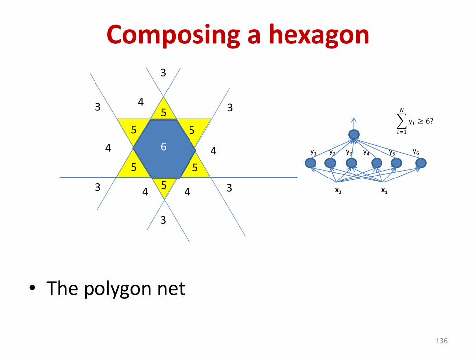
Composing a hexagon
• The polygon net
136
6
5
5
5
5
5
5
x1x2
𝑖=1
𝑁
y𝑖 ≥ 6?
y1 y5y2 y3 y4 y6
3
3
3
3
3
3
4
4
4
44
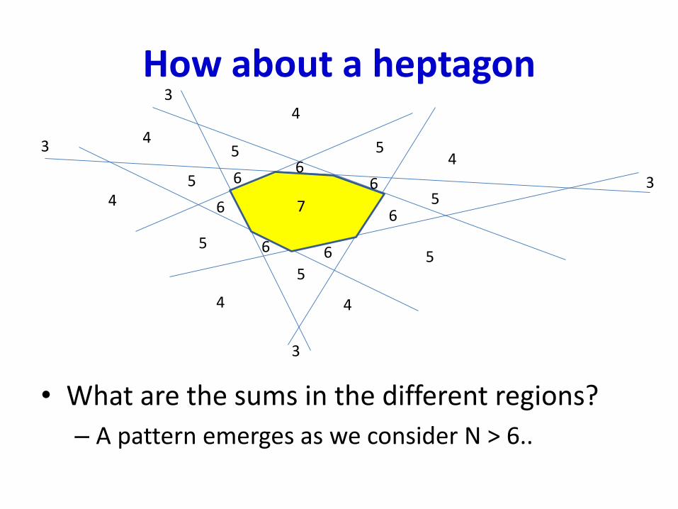
How about a heptagon
• What are the sums in the different regions?
– A pattern emerges as we consider N > 6..
4
7
66
6
66
6
6
5
5
5
5
5
5
4
4 4
5
4
43
3
3
3
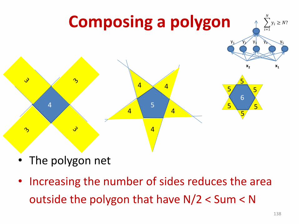
Composing a polygon
• The polygon net
• Increasing the number of sides reduces the area
outside the polygon that have N/2 < Sum < N138
4 56
44
4
4
4
55
55
5
5
x1x2
𝑖=1
𝑁
y𝑖 ≥ 𝑁?
y1 y5y2 y3 y4
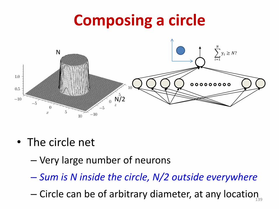
Composing a circle
• The circle net
– Very large number of neurons
– Sum is N inside the circle, N/2 outside everywhere
– Circle can be of arbitrary diameter, at any location139
N
N/2
𝑖=1
𝑁
y𝑖 ≥ 𝑁?
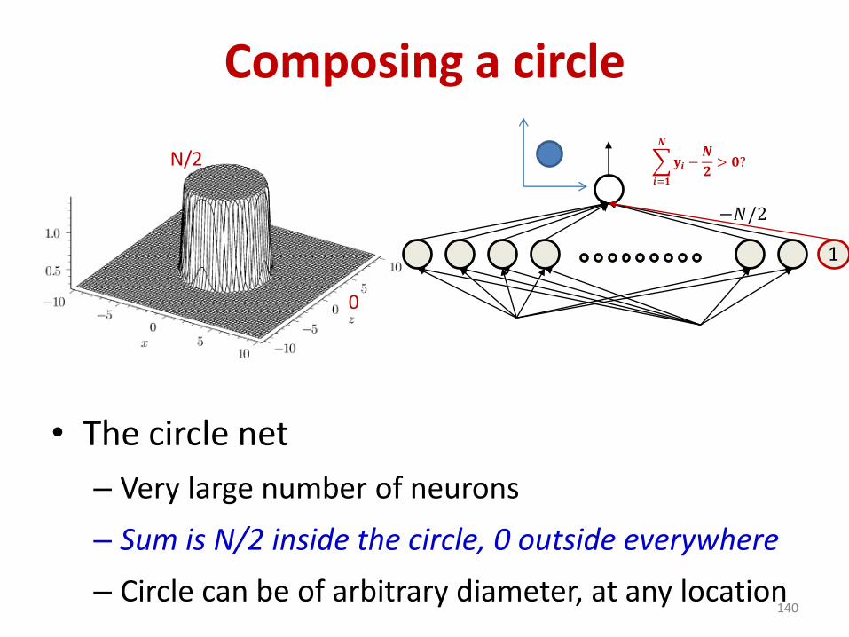
Composing a circle
• The circle net
– Very large number of neurons
– Sum is N/2 inside the circle, 0 outside everywhere
– Circle can be of arbitrary diameter, at any location140
N/2
0
𝒊=𝟏
𝑵
𝐲𝒊 −𝑵
𝟐> 𝟎?
1
−𝑁/2
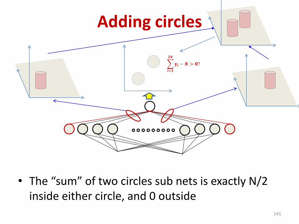
Adding circles
• The “sum” of two circles sub nets is exactly N/2 inside either circle, and 0 outside
141
𝒊=𝟏
𝟐𝑵
𝐲𝒊 −𝑵 > 𝟎?
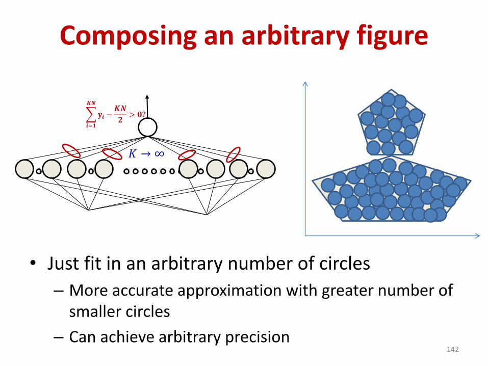
Composing an arbitrary figure
• Just fit in an arbitrary number of circles
– More accurate approximation with greater number of smaller circles
– Can achieve arbitrary precision142
𝒊=𝟏
𝑲𝑵
𝐲𝒊 −𝑲𝑵
𝟐> 𝟎?
𝐾 → ∞
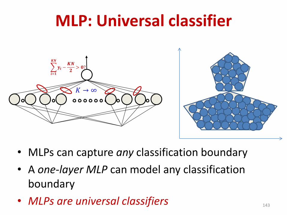
MLP: Universal classifier
• MLPs can capture any classification boundary
• A one-layer MLP can model any classification boundary
• MLPs are universal classifiers 143
𝒊=𝟏
𝑲𝑵
𝐲𝒊 −𝑲𝑵
𝟐> 𝟎?
𝐾 → ∞
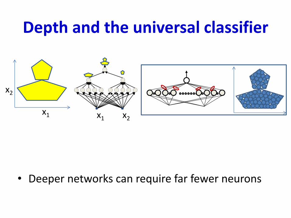
Depth and the universal classifier
• Deeper networks can require far fewer neurons
x2
x1 x1 x2
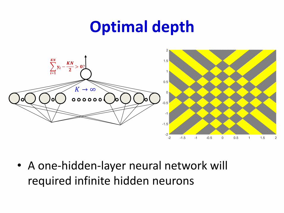
Optimal depth
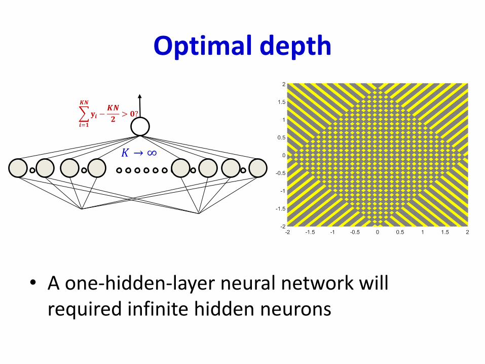
• A one-hidden-layer neural network will required infinite hidden neurons
𝒊=𝟏
𝑲𝑵
𝐲𝒊 −𝑲𝑵
𝟐> 𝟎?
𝐾 → ∞
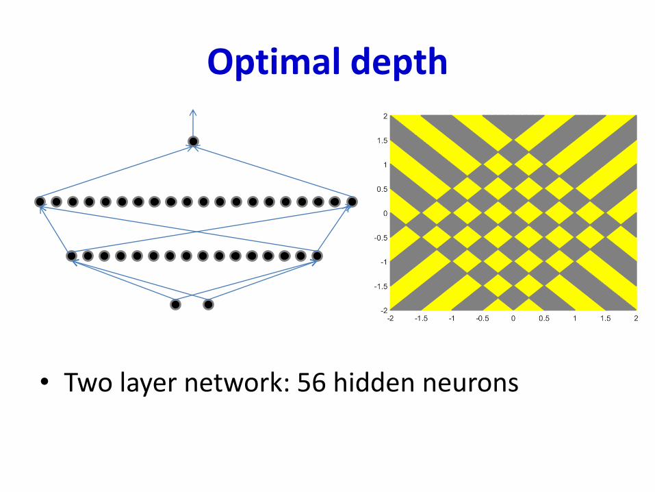
Optimal depth
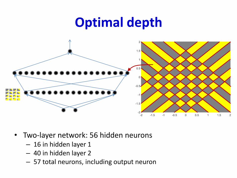
• Two layer network: 56 hidden neurons
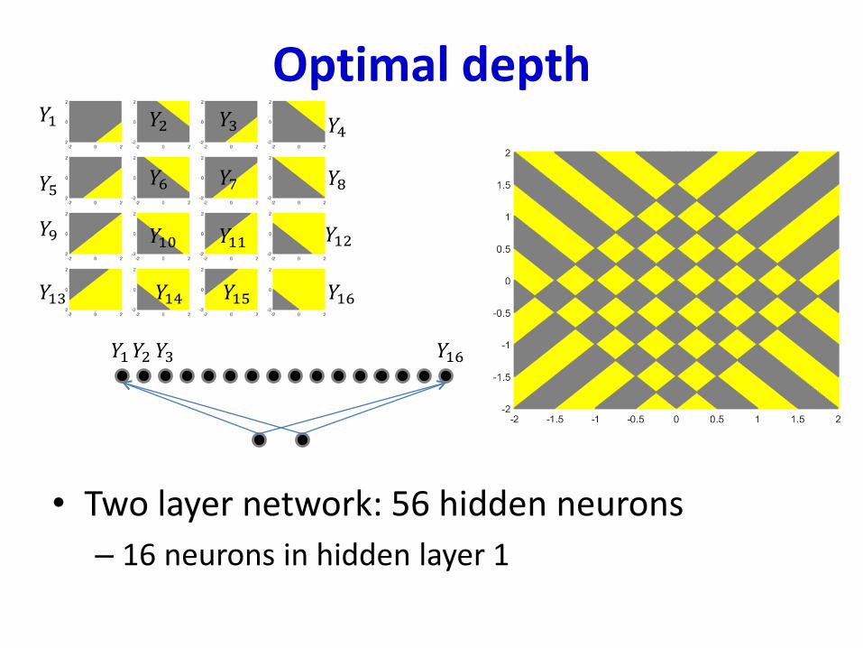
Optimal depth
• Two layer network: 56 hidden neurons
– 16 neurons in hidden layer 1
𝑌1𝑌2 𝑌3 𝑌16
𝑌16
𝑌1 𝑌2 𝑌3 𝑌4
𝑌5 𝑌8
𝑌9 𝑌12
𝑌13 𝑌14 𝑌15
𝑌6 𝑌7
𝑌10 𝑌11
Optimal depth
• Two-layer network: 56 hidden neurons– 16 in hidden layer 1– 40 in hidden layer 2– 57 total neurons, including output neuron
Optimal depth
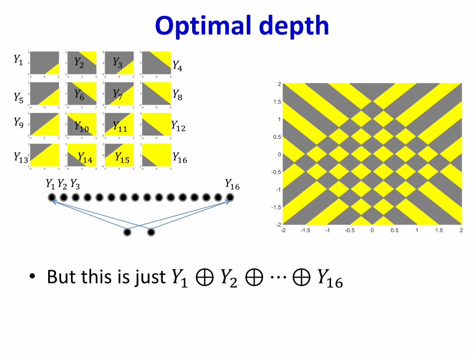
• But this is just 𝑌1⊕𝑌2 ⊕⋯⊕𝑌16
𝑌1𝑌2 𝑌3 𝑌16
𝑌16
𝑌1 𝑌2 𝑌3 𝑌4
𝑌5 𝑌8
𝑌9 𝑌12
𝑌13 𝑌14 𝑌15
𝑌6 𝑌7
𝑌10 𝑌11
Optimal depth
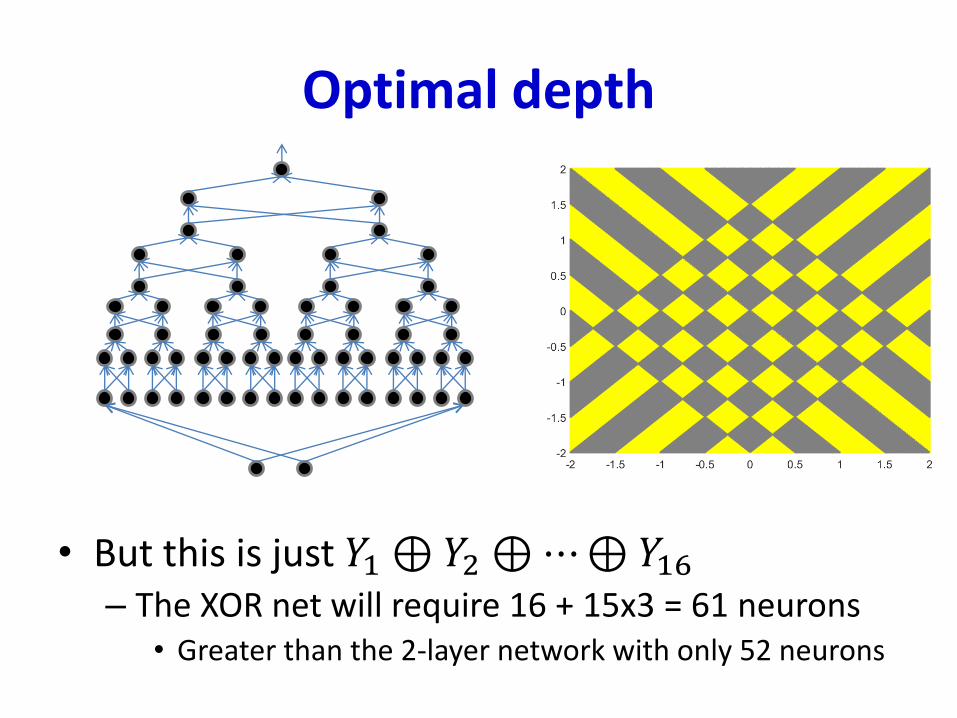
• But this is just 𝑌1⊕𝑌2 ⊕⋯⊕𝑌16– The XOR net will require 16 + 15x3 = 61 neurons
• Greater than the 2-layer network with only 52 neurons
Optimal depth
• A one-hidden-layer neural network will required infinite hidden neurons
𝒊=𝟏
𝑲𝑵
𝐲𝒊 −𝑲𝑵
𝟐> 𝟎?
𝐾 → ∞
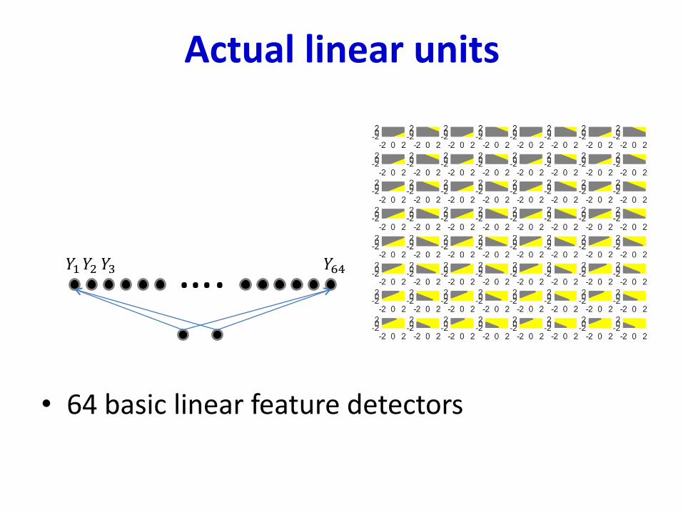
Actual linear units
• 64 basic linear feature detectors
𝑌1𝑌2 𝑌3 𝑌64….
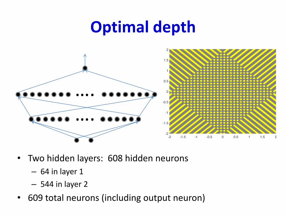
Optimal depth
• Two hidden layers: 608 hidden neurons
– 64 in layer 1
– 544 in layer 2
• 609 total neurons (including output neuron)
….….
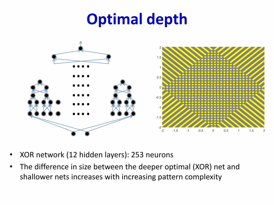
Optimal depth
• XOR network (12 hidden layers): 253 neurons
• The difference in size between the deeper optimal (XOR) net and shallower nets increases with increasing pattern complexity
….….….….….….
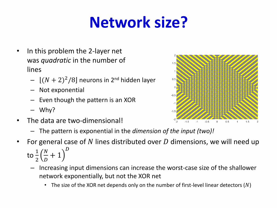
Network size?
• In this problem the 2-layer netwas quadratic in the number oflines
– (𝑁 + 2)2/8 neurons in 2nd hidden layer
– Not exponential
– Even though the pattern is an XOR
– Why?
• The data are two-dimensional!
– The pattern is exponential in the dimension of the input (two)!
• For general case of 𝑁 lines distributed over 𝐷 dimensions, we will need up
to 1
2
𝑁
𝐷+ 1
𝐷
– Increasing input dimensions can increase the worst-case size of the shallower network exponentially, but not the XOR net• The size of the XOR net depends only on the number of first-level linear detectors (𝑁)
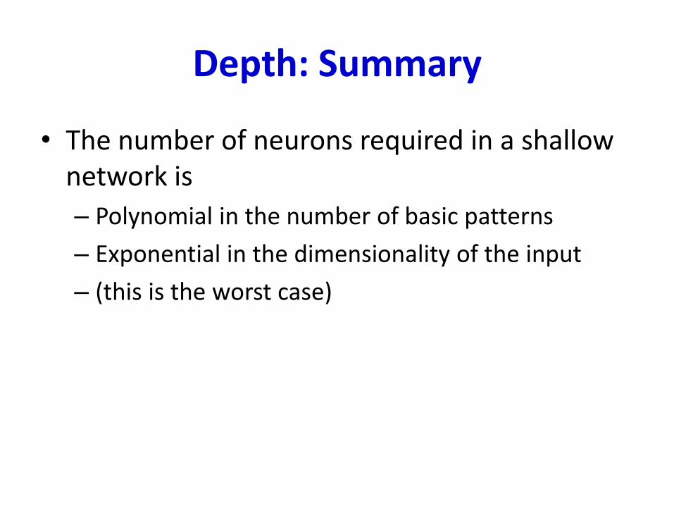
Depth: Summary
• The number of neurons required in a shallow network is
– Polynomial in the number of basic patterns
– Exponential in the dimensionality of the input
– (this is the worst case)
Story so far
• Multi-layer perceptrons are Universal Boolean Machines– Even a network with a single hidden layer is a universal Boolean machine
• Multi-layer perceptrons are Universal Classification Functions– Even a network with a single hidden layer is a universal classifier
• But a single-layer network may require an exponentially large number of perceptrons than a deep one
• Deeper networks may require exponentially fewer neurons than shallower networks to express the same function– Could be exponentially smaller
– Deeper networks are more expressive
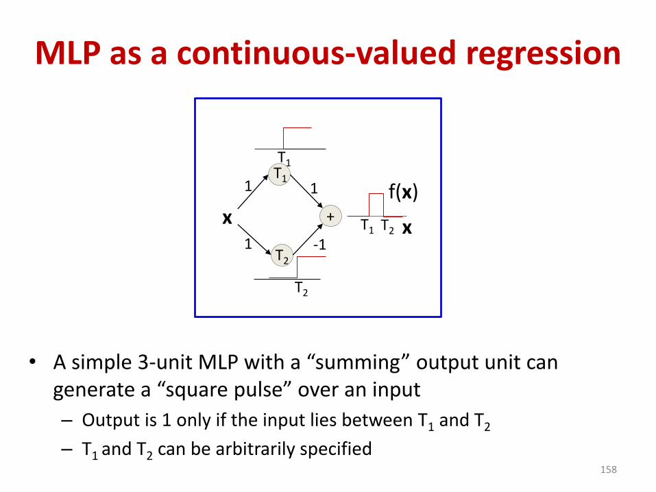
MLP as a continuous-valued regression
• A simple 3-unit MLP with a “summing” output unit can generate a “square pulse” over an input
– Output is 1 only if the input lies between T1 and T2
– T1 and T2 can be arbitrarily specified158
+x
1T1
T2
1
T1
T2
1
-1T1 T2 x
f(x)
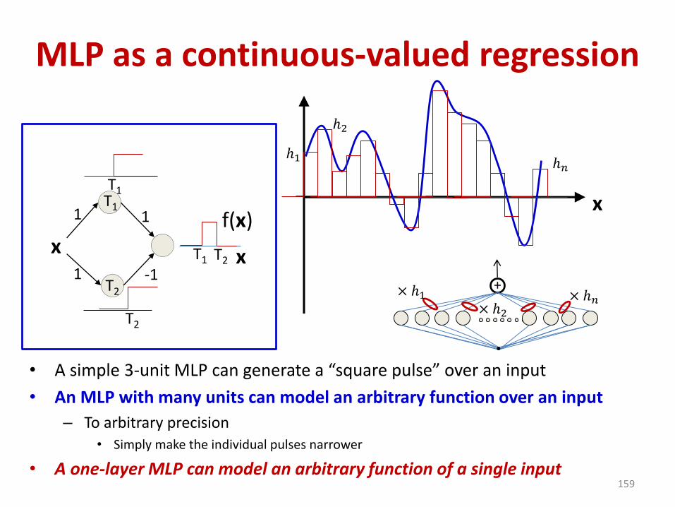
MLP as a continuous-valued regression
• A simple 3-unit MLP can generate a “square pulse” over an input
• An MLP with many units can model an arbitrary function over an input
– To arbitrary precision• Simply make the individual pulses narrower
• A one-layer MLP can model an arbitrary function of a single input159
x
1T1
T2
1
T1
T2
1
-1T1 T2 x
f(x)x
+× ℎ1× ℎ2
× ℎ𝑛
ℎ1
ℎ2
ℎ𝑛
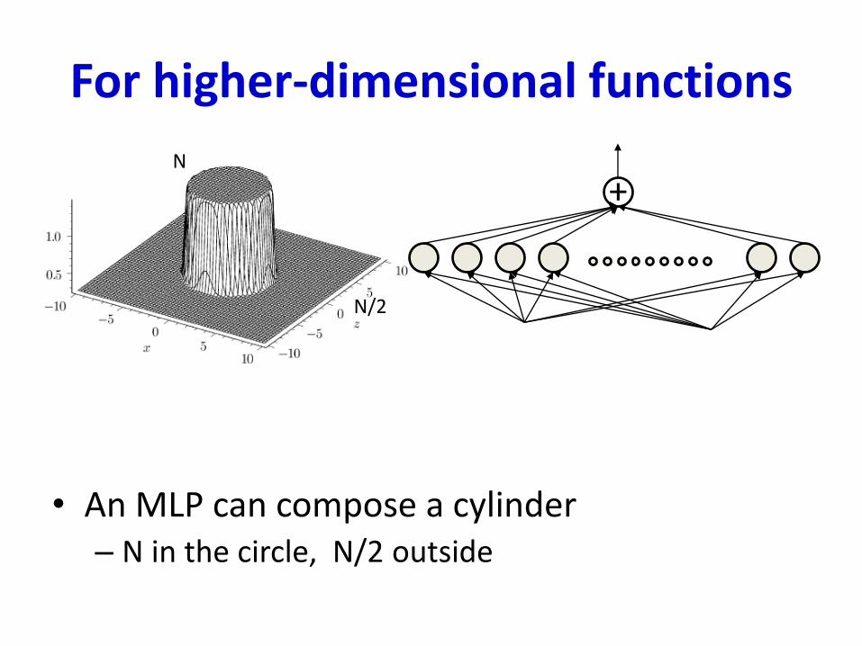
For higher-dimensional functions
• An MLP can compose a cylinder– N in the circle, N/2 outside
N
N/2
+
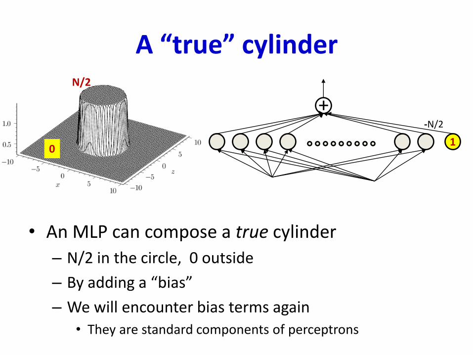
A “true” cylinder
• An MLP can compose a true cylinder
– N/2 in the circle, 0 outside
– By adding a “bias”
– We will encounter bias terms again
• They are standard components of perceptrons
N/2
0
+
1
-N/2
+
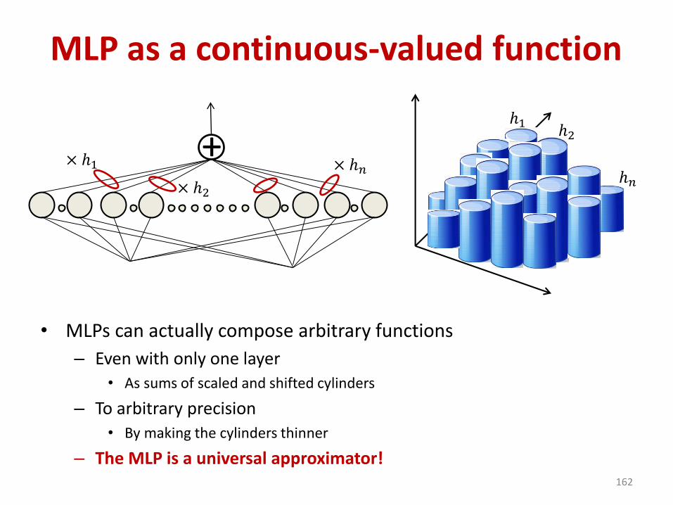
MLP as a continuous-valued function
• MLPs can actually compose arbitrary functions
– Even with only one layer
• As sums of scaled and shifted cylinders
– To arbitrary precision
• By making the cylinders thinner
– The MLP is a universal approximator!162
× ℎ1
× ℎ2
× ℎ𝑛
ℎ1ℎ2
ℎ𝑛
The issue of depth
• Previous discussion showed that a single-layer MLP is a universal function approximator
– Can approximate any function to arbitrary precision
– But may require infinite neurons in the layer
• More generally, deeper networks will require far fewer neurons for the same approximation error
– The network is a generic map• The same principles that apply for Boolean networks apply here
– Can be exponentially fewer than the 1-layer network
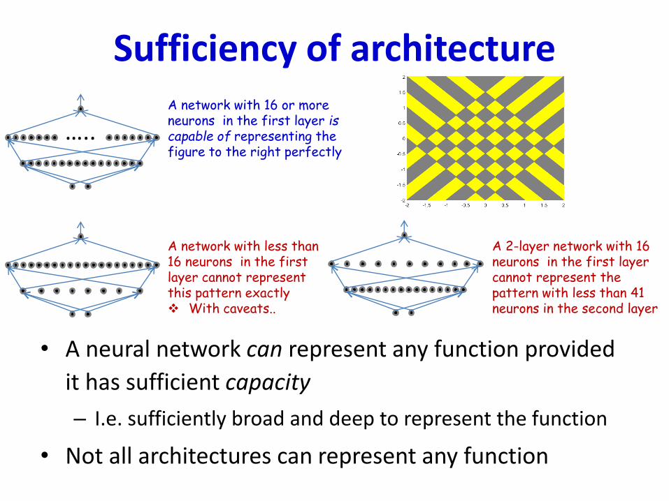
Sufficiency of architecture
• A neural network can represent any function provided
it has sufficient capacity
– I.e. sufficiently broad and deep to represent the function
• Not all architectures can represent any function
A network with 16 or moreneurons in the first layer is capable of representing the figure to the right perfectly
A network with less than 16 neurons in the first layer cannot represent this pattern exactly With caveats..
…..
A 2-layer network with 16 neurons in the first layer cannot represent the pattern with less than 41neurons in the second layer
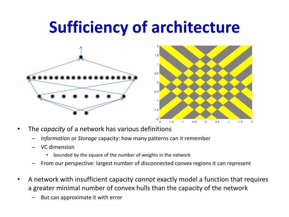
Sufficiency of architecture
• The capacity of a network has various definitions– Information or Storage capacity: how many patterns can it remember
– VC dimension
• bounded by the square of the number of weights in the network
– From our perspective: largest number of disconnected convex regions it can represent
• A network with insufficient capacity cannot exactly model a function that requires a greater minimal number of convex hulls than the capacity of the network– But can approximate it with error
Lessons
• MLPs are universal Boolean function
• MLPs are universal classifiers
• MLPs are universal function approximators
• A single-layer MLP can approximate anything to arbitrary precision
– But could be exponentially or even infinitely wide in its inputs size
• Deeper MLPs can achieve the same precision with far fewer neurons
– Deeper networks are more expressive
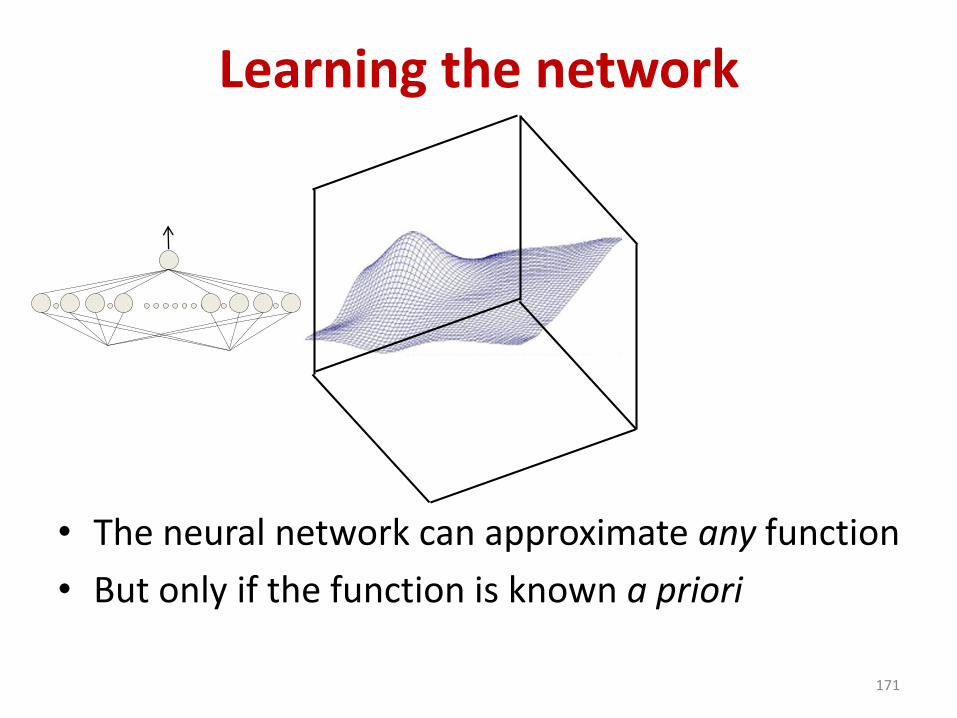
Learning the network
• The neural network can approximate any function
• But only if the function is known a priori
171
Learning the network
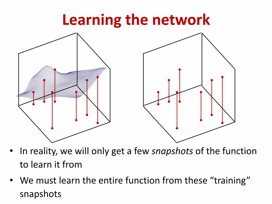
• In reality, we will only get a few snapshots of the function
to learn it from
• We must learn the entire function from these “training”
snapshots
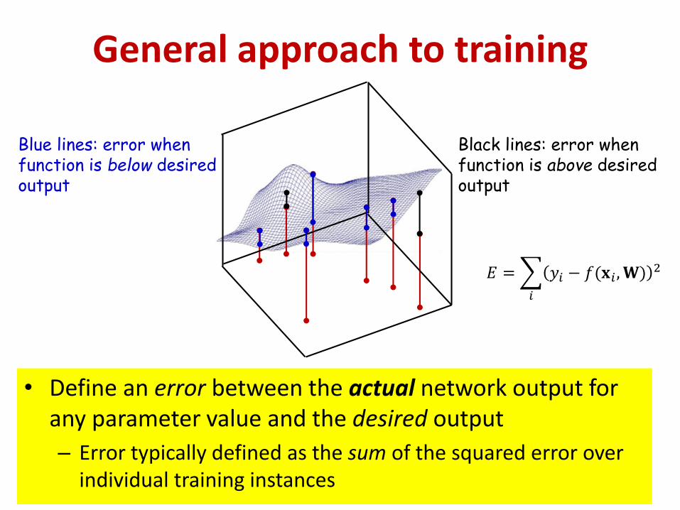
General approach to training
• Define an error between the actual network output for any parameter value and the desired output
– Error typically defined as the sum of the squared error over individual training instances
Blue lines: error whenfunction is below desiredoutput
Black lines: error whenfunction is above desiredoutput
𝐸 =
𝑖
𝑦𝑖 − 𝑓(𝐱𝑖 ,𝐖) 2
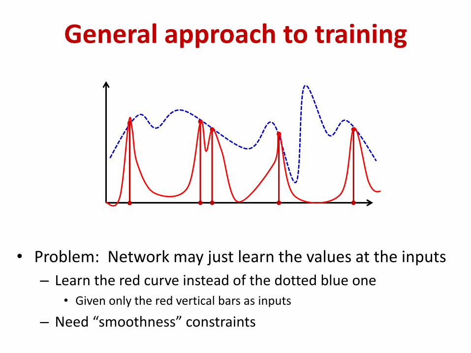
General approach to training
• Problem: Network may just learn the values at the inputs
– Learn the red curve instead of the dotted blue one• Given only the red vertical bars as inputs
– Need “smoothness” constraints
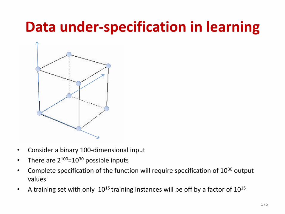
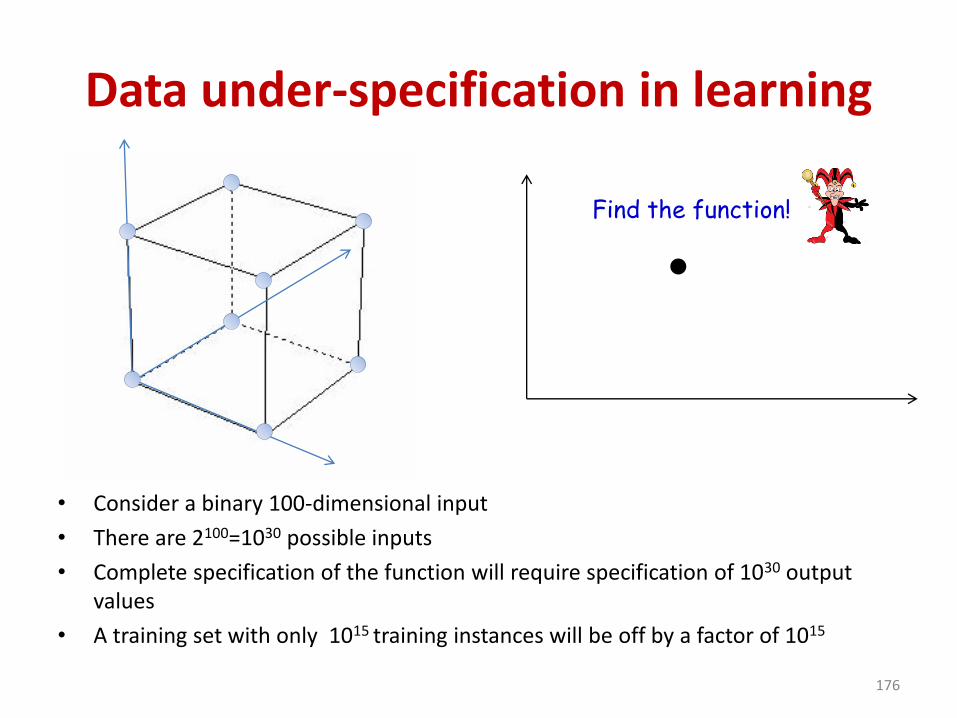
Data under-specification in learning
• Consider a binary 100-dimensional input
• There are 2100=1030 possible inputs
• Complete specification of the function will require specification of 1030 output values
• A training set with only 1015 training instances will be off by a factor of 1015
175
Data under-specification in learning
• Consider a binary 100-dimensional input
• There are 2100=1030 possible inputs
• Complete specification of the function will require specification of 1030 output values
• A training set with only 1015 training instances will be off by a factor of 1015
176
Find the function!
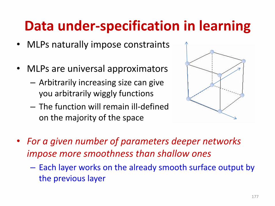
Data under-specification in learning• MLPs naturally impose constraints
• MLPs are universal approximators
– Arbitrarily increasing size can give you arbitrarily wiggly functions
– The function will remain ill-defined on the majority of the space
• For a given number of parameters deeper networks impose more smoothness than shallow ones
– Each layer works on the already smooth surface output by the previous layer
177
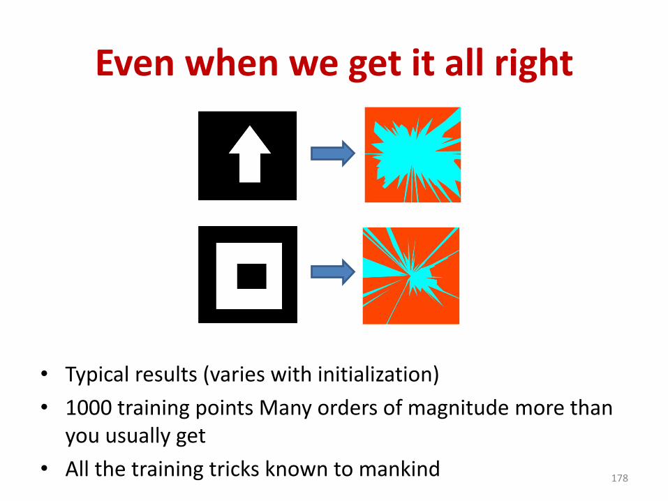
• Typical results (varies with initialization)
• 1000 training points Many orders of magnitude more than you usually get
• All the training tricks known to mankind 178
Even when we get it all right
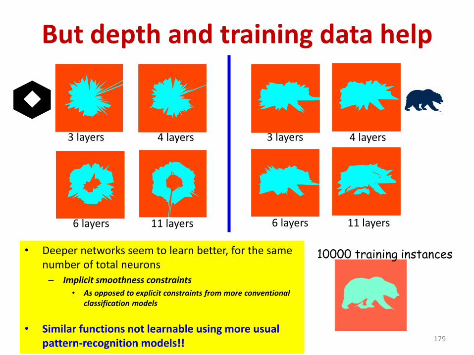
But depth and training data help
• Deeper networks seem to learn better, for the same number of total neurons– Implicit smoothness constraints
• As opposed to explicit constraints from more conventional classification models
• Similar functions not learnable using more usual pattern-recognition models!! 179
6 layers 11 layers
3 layers 4 layers
6 layers 11 layers
3 layers 4 layers
10000 training instances
Part 3: Learning the network
NNets in AI
• The network is a function
– Given an input, it computes the function layer wise to predict an output
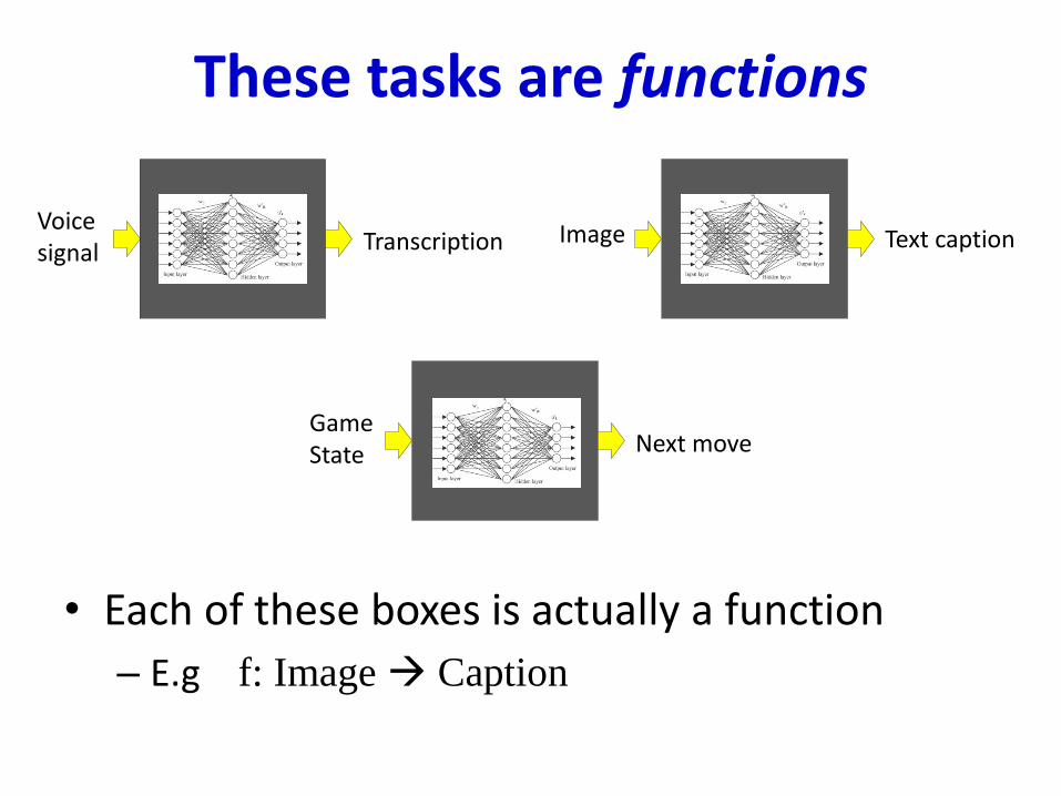
These tasks are functions
• Each of these boxes is actually a function
– E.g f: Image Caption
N.NetVoice signal Transcription N.NetImage Text caption
N.NetGameState Next move
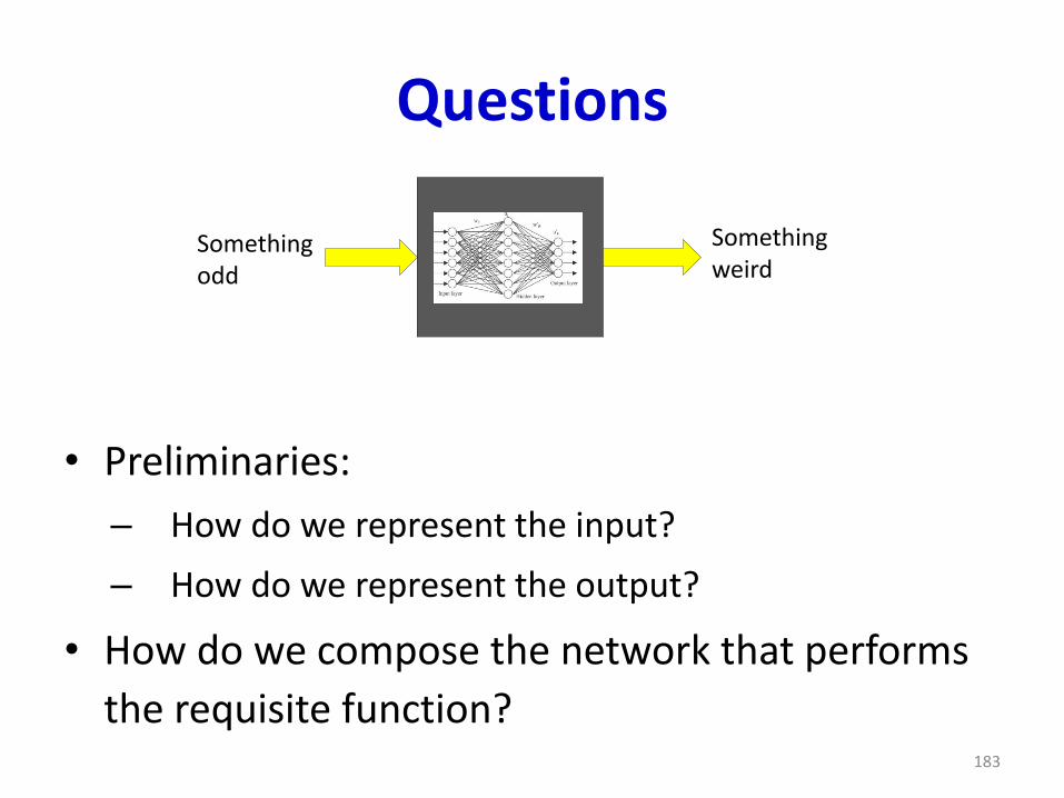
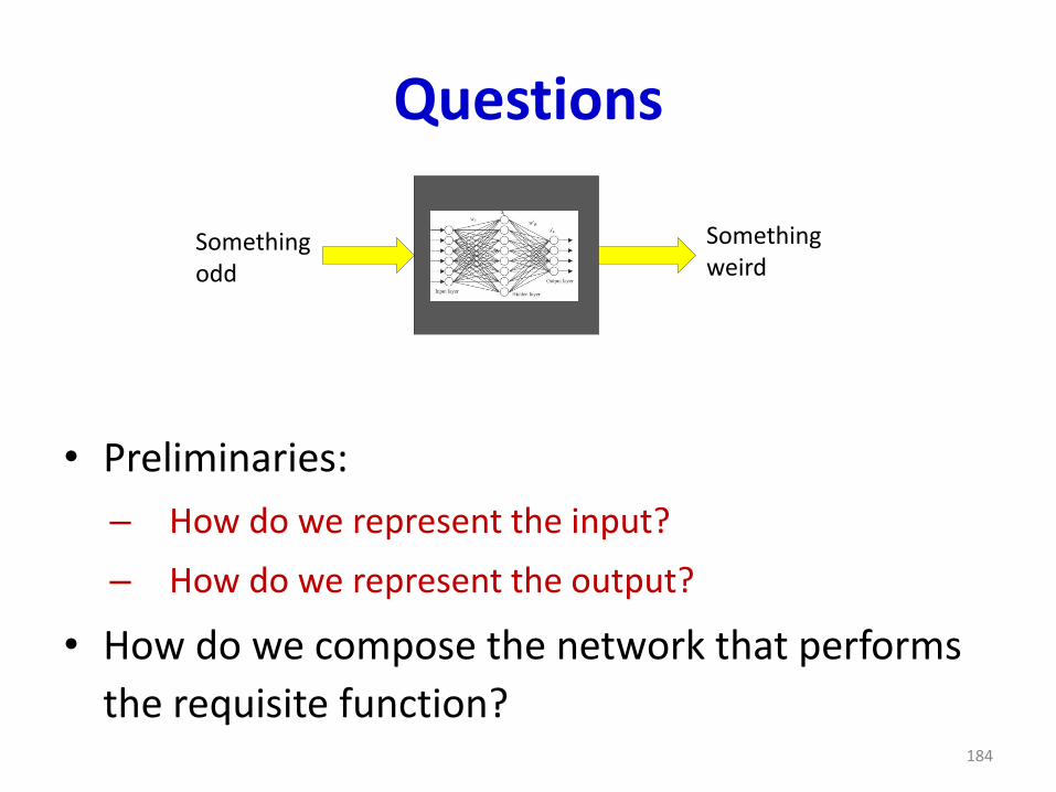
Questions
• Preliminaries:
– How do we represent the input?
– How do we represent the output?
• How do we compose the network that performs
the requisite function?183
N.NetSomethingodd
Somethingweird
Questions
• Preliminaries:
– How do we represent the input?
– How do we represent the output?
• How do we compose the network that performs
the requisite function?184
N.NetSomethingodd
Somethingweird
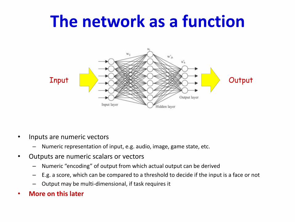
The network as a function
• Inputs are numeric vectors– Numeric representation of input, e.g. audio, image, game state, etc.
• Outputs are numeric scalars or vectors– Numeric “encoding” of output from which actual output can be derived
– E.g. a score, which can be compared to a threshold to decide if the input is a face or not
– Output may be multi-dimensional, if task requires it
Input Output
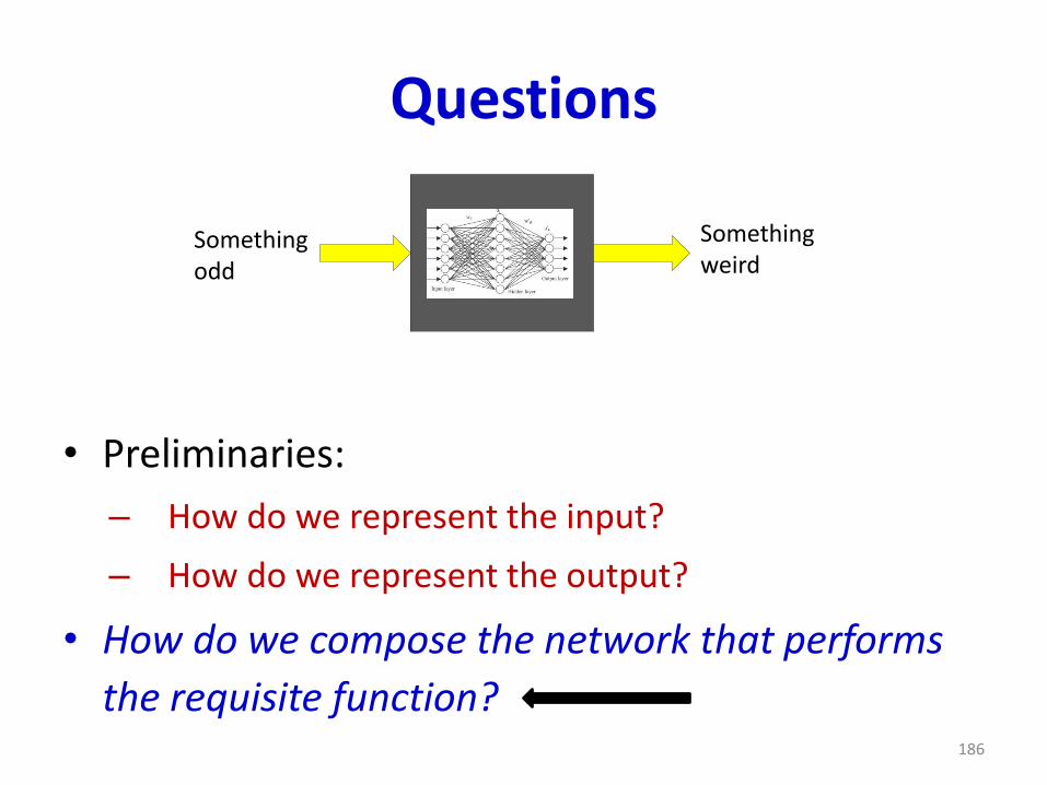
Questions
• Preliminaries:
– How do we represent the input?
– How do we represent the output?
• How do we compose the network that performs
the requisite function?186
N.NetSomethingodd
Somethingweird
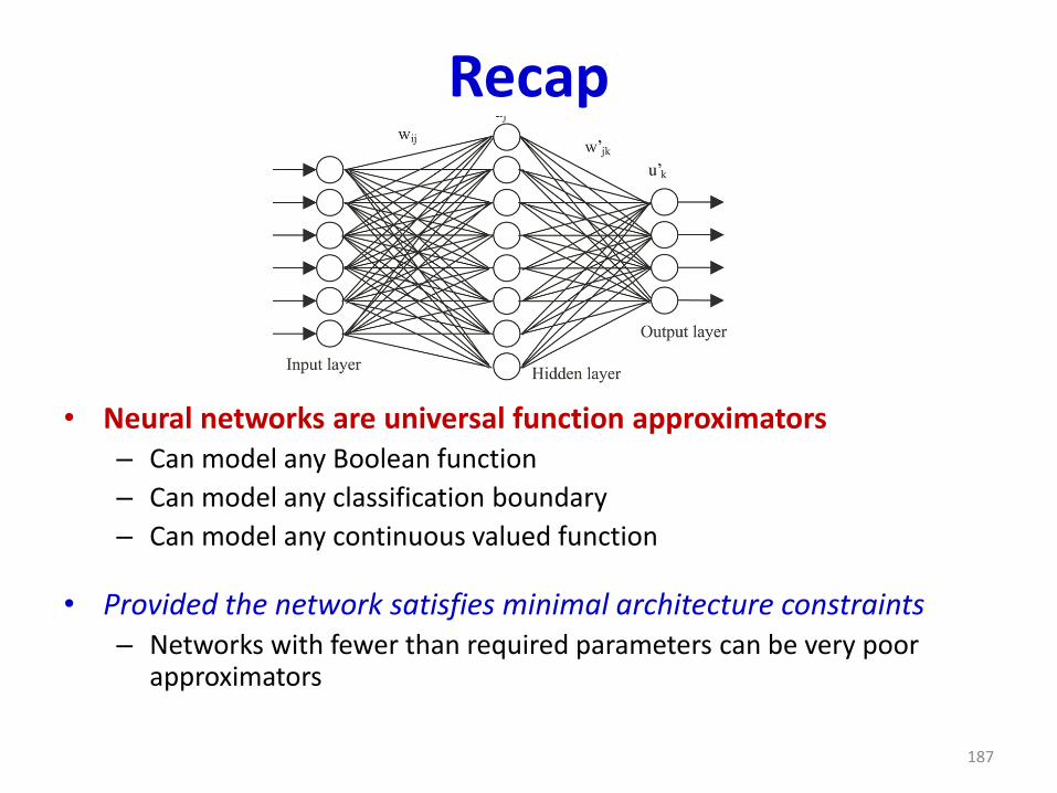
Recap
• Neural networks are universal function approximators– Can model any Boolean function
– Can model any classification boundary
– Can model any continuous valued function
• Provided the network satisfies minimal architecture constraints– Networks with fewer than required parameters can be very poor
approximators
187
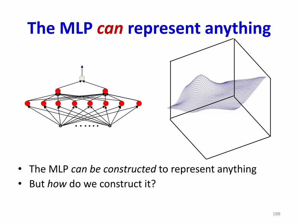
The MLP can represent anything
• The MLP can be constructed to represent anything
• But how do we construct it?
188
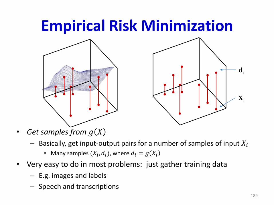
Empirical Risk Minimization
• Get samples from 𝑔 𝑋
– Basically, get input-output pairs for a number of samples of input 𝑋𝑖• Many samples (𝑋𝑖, 𝑑𝑖), where 𝑑𝑖 = 𝑔 𝑋𝑖
• Very easy to do in most problems: just gather training data
– E.g. images and labels
– Speech and transcriptions189
Xi
di
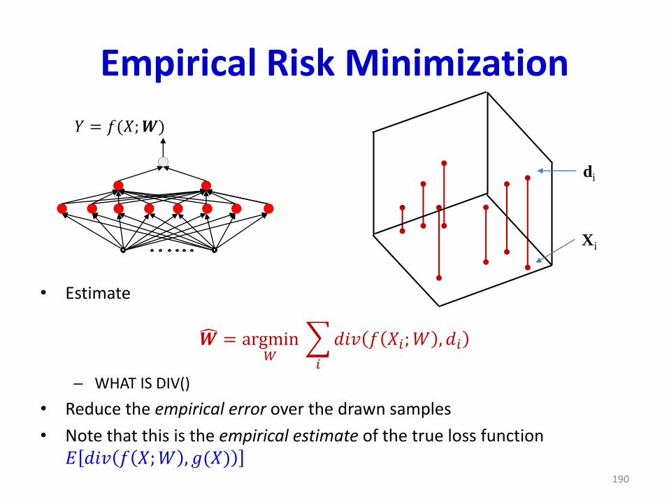
Empirical Risk Minimization
• Estimate
𝑾 = argmin𝑊
𝑖
𝑑𝑖𝑣 𝑓 𝑋𝑖;𝑊 , 𝑑𝑖
– WHAT IS DIV()
• Reduce the empirical error over the drawn samples
• Note that this is the empirical estimate of the true loss function 𝐸 𝑑𝑖𝑣 𝑓 𝑋;𝑊 , 𝑔(𝑋)
190
Xi
di
𝑌 = 𝑓(𝑋;𝑾)
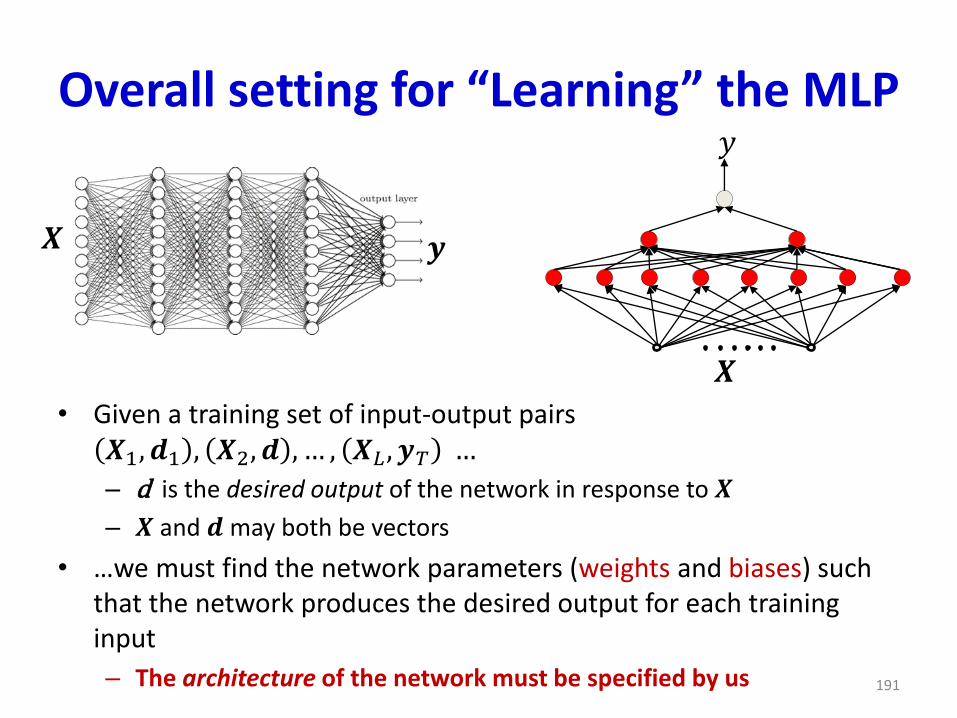
Overall setting for “Learning” the MLP
• Given a training set of input-output pairs 𝑿1, 𝒅1 , 𝑿2, 𝒅 , … , 𝑿𝐿 , 𝒚𝑇 …
– d is the desired output of the network in response to 𝑿
– 𝑿 and 𝒅 may both be vectors
• …we must find the network parameters (weights and biases) such that the network produces the desired output for each training input
– The architecture of the network must be specified by us
𝑦
𝑿
𝑿 𝒚
191
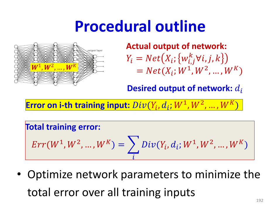
Procedural outline
• Optimize network parameters to minimize the
total error over all training inputs
Actual output of network:
𝑌𝑖 = 𝑁𝑒𝑡 𝑋𝑖; 𝑤𝑖,𝑗𝑘 ∀𝑖, 𝑗, 𝑘
= 𝑁𝑒𝑡(𝑋𝑖;𝑊1,𝑊2, … ,𝑊𝐾)
Desired output of network: 𝑑𝑖
Error on i-th training input: 𝐷𝑖𝑣(𝑌𝑖 , 𝑑𝑖;𝑊1,𝑊2, … ,𝑊𝐾)
𝑾1,𝑾2, … ,𝑾𝐾
Total training error:
𝐸𝑟𝑟(𝑊1,𝑊2, … ,𝑊𝐾) =
𝑖
𝐷𝑖𝑣(𝑌𝑖 , 𝑑𝑖;𝑊1,𝑊2, … ,𝑊𝐾)
192
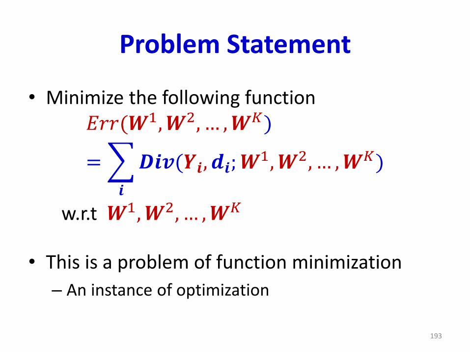
Problem Statement
• Minimize the following function𝐸𝑟𝑟(𝑾1,𝑾2, … ,𝑾𝐾)
=
𝒊
𝑫𝒊𝒗(𝒀𝒊, 𝒅𝒊;𝑾1,𝑾2, … ,𝑾𝐾)
w.r.t 𝑾1,𝑾2, … ,𝑾𝐾
• This is a problem of function minimization
– An instance of optimization
193
• A CRASH COURSE ON FUNCTION OPTIMIZATION
194
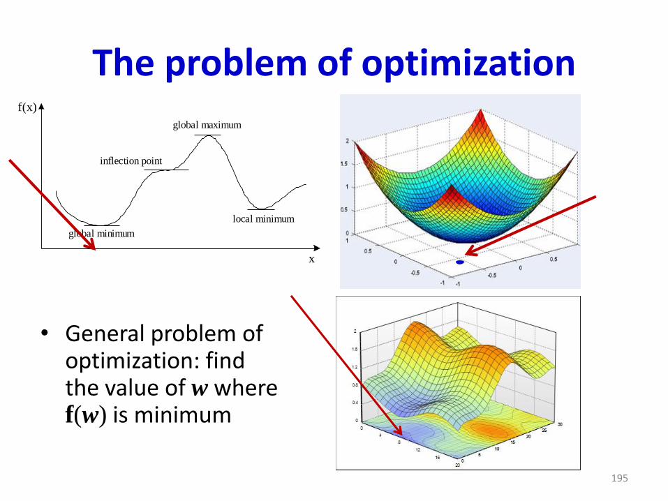
The problem of optimization
• General problem of optimization: find the value of w where f(w) is minimum
f(x)
x
global minimum
inflection point
local minimum
global maximum
195
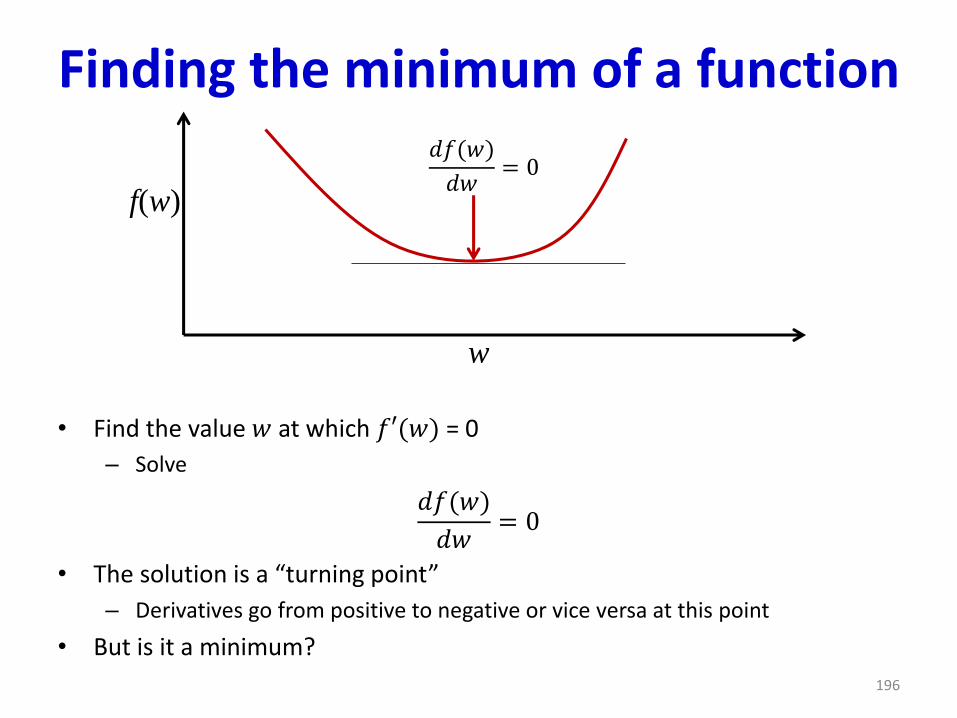
Finding the minimum of a function
• Find the value 𝑤 at which 𝑓′(𝑤) = 0
– Solve
𝑑𝑓(𝑤)
𝑑𝑤= 0
• The solution is a “turning point”
– Derivatives go from positive to negative or vice versa at this point
• But is it a minimum?
196
w
f(w)
𝑑𝑓(𝑤)
𝑑𝑤= 0
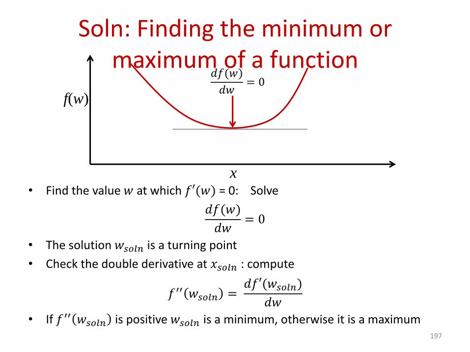
Soln: Finding the minimum or maximum of a function
• Find the value 𝑤 at which 𝑓′(𝑤) = 0: Solve
𝑑𝑓(𝑤)
𝑑𝑤= 0
• The solution 𝑤𝑠𝑜𝑙𝑛 is a turning point
• Check the double derivative at 𝑥𝑠𝑜𝑙𝑛 : compute
𝑓′′ 𝑤𝑠𝑜𝑙𝑛 =𝑑𝑓′(𝑤𝑠𝑜𝑙𝑛)
𝑑𝑤
• If 𝑓′′ 𝑤𝑠𝑜𝑙𝑛 is positive 𝑤𝑠𝑜𝑙𝑛 is a minimum, otherwise it is a maximum197
x
f(w)
𝑑𝑓(𝑤)
𝑑𝑤= 0
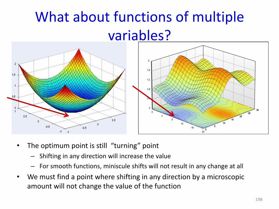
What about functions of multiple variables?
• The optimum point is still “turning” point
– Shifting in any direction will increase the value
– For smooth functions, miniscule shifts will not result in any change at all
• We must find a point where shifting in any direction by a microscopic amount will not change the value of the function
198
A brief note on derivatives of multivariate functions
199
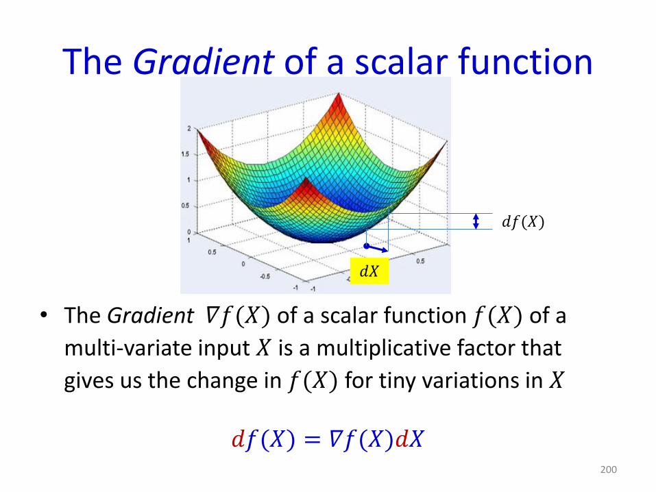
The Gradient of a scalar function
• The Gradient 𝛻𝑓(𝑋) of a scalar function 𝑓(𝑋) of a
multi-variate input 𝑋 is a multiplicative factor that
gives us the change in 𝑓(𝑋) for tiny variations in 𝑋
𝑑𝑓(𝑋) = 𝛻𝑓(𝑋)𝑑𝑋200
𝑑𝑓(𝑋)
𝑑𝑋
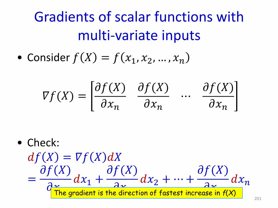
Gradients of scalar functions with multi-variate inputs
• Consider 𝑓 𝑋 = 𝑓 𝑥1, 𝑥2, … , 𝑥𝑛
𝛻𝑓(𝑋) =𝜕𝑓(𝑋)
𝜕𝑥𝑛
𝜕𝑓(𝑋)
𝜕𝑥𝑛⋯
𝜕𝑓(𝑋)
𝜕𝑥𝑛
• Check:𝑑𝑓 𝑋 = 𝛻𝑓 𝑋 𝑑𝑋
=𝜕𝑓(𝑋)
𝜕𝑥1𝑑𝑥1 +
𝜕𝑓(𝑋)
𝜕𝑥2𝑑𝑥2 +⋯+
𝜕𝑓(𝑋)
𝜕𝑥𝑛𝑑𝑥𝑛
201The gradient is the direction of fastest increase in f(X)
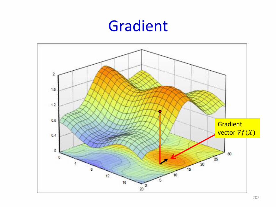
Gradient
202
Gradientvector 𝛻𝑓(𝑋)
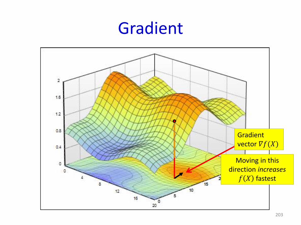
Gradient
203
Gradientvector 𝛻𝑓(𝑋)
Moving in this direction increases
𝑓 𝑋 fastest
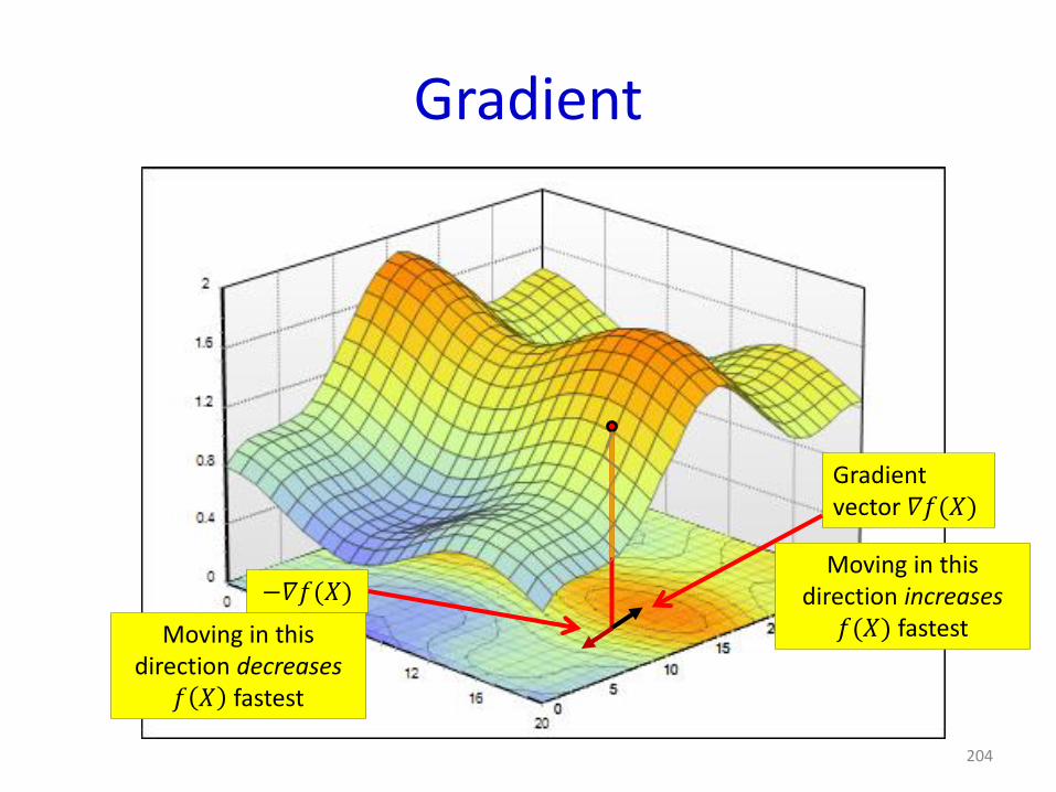
Gradient
204
Gradientvector 𝛻𝑓(𝑋)
Moving in this direction increases
𝑓(𝑋) fastest
−𝛻𝑓(𝑋)
Moving in this direction decreases
𝑓 𝑋 fastest
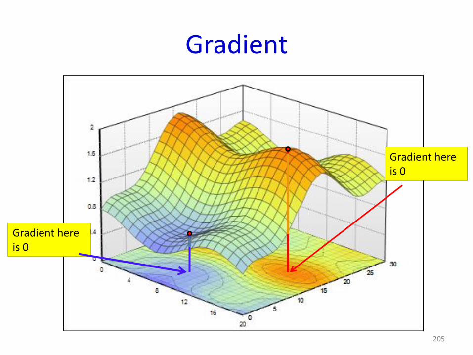
Gradient
205
Gradient hereis 0
Gradient hereis 0
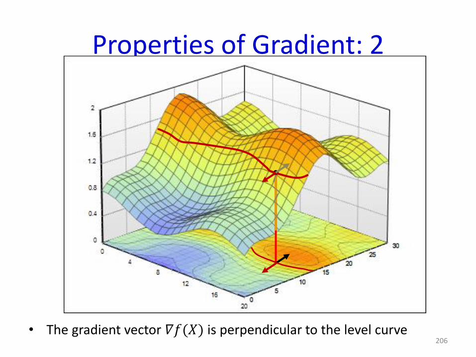
Properties of Gradient: 2
• The gradient vector 𝛻𝑓(𝑋) is perpendicular to the level curve206
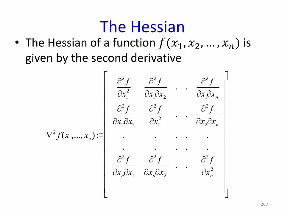
The Hessian• The Hessian of a function 𝑓(𝑥1, 𝑥2, … , 𝑥𝑛) is
given by the second derivative
207
Ñ2 f (x1,..., xn ) :=
¶2 f
¶x1
2
¶2 f
¶x1¶x2
. .¶2 f
¶x1¶xn
¶2 f
¶x2¶x1
¶2 f
¶x2
2. .
¶2 f
¶x2¶xn
. . . . .
. . . . .
¶2 f
¶xn¶x1
¶2 f
¶xn¶x2
. .¶2 f
¶xn2
é
ë
êêêêêêêêêêêêê
ù
û
úúúúúúúúúúúúú
Returning to direct optimization…
208
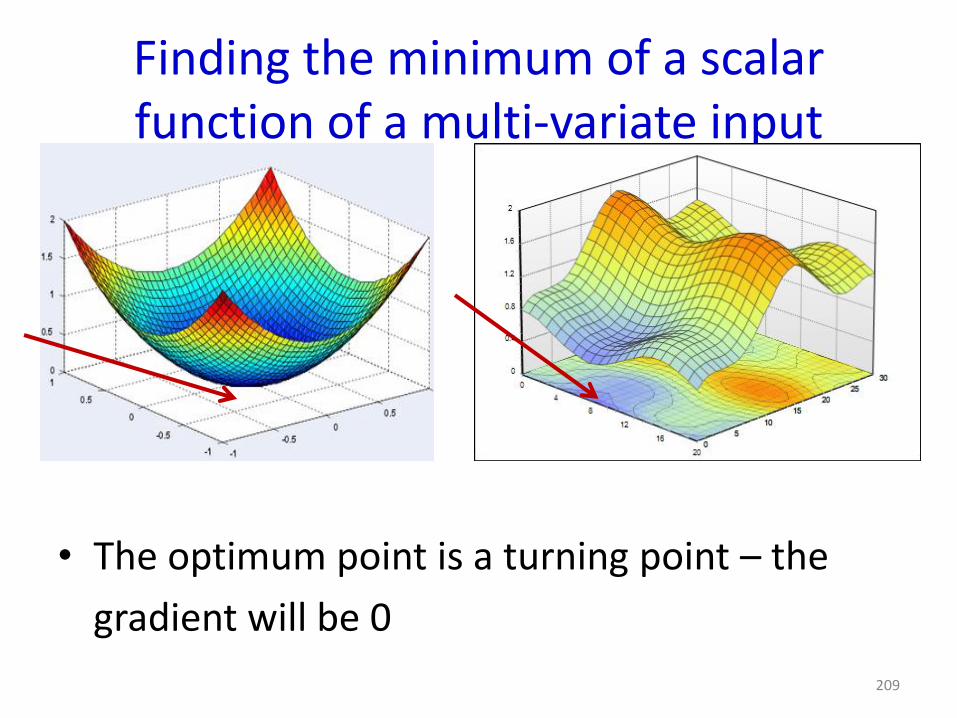
Finding the minimum of a scalar function of a multi-variate input
• The optimum point is a turning point – the
gradient will be 0
209
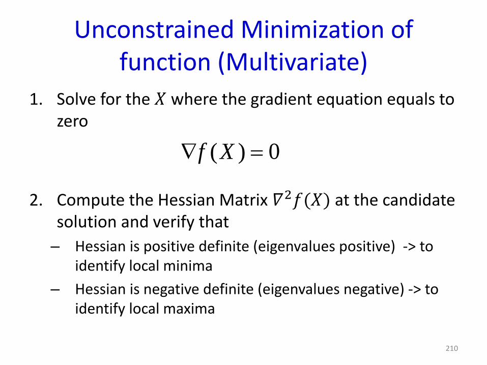
Unconstrained Minimization of function (Multivariate)
1. Solve for the 𝑋 where the gradient equation equals to zero
2. Compute the Hessian Matrix 𝛻2𝑓(𝑋) at the candidate solution and verify that
– Hessian is positive definite (eigenvalues positive) -> to identify local minima
– Hessian is negative definite (eigenvalues negative) -> to identify local maxima
210
0)( Xf
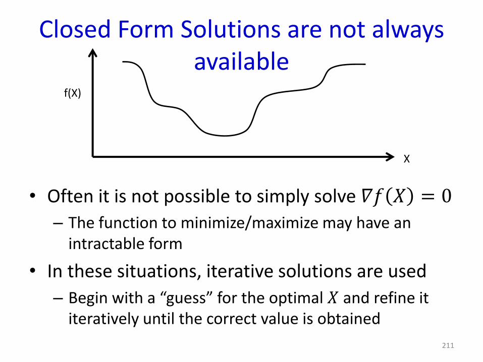
Closed Form Solutions are not always available
• Often it is not possible to simply solve 𝛻𝑓 𝑋 = 0
– The function to minimize/maximize may have an intractable form
• In these situations, iterative solutions are used
– Begin with a “guess” for the optimal 𝑋 and refine it iteratively until the correct value is obtained
211
X
f(X)
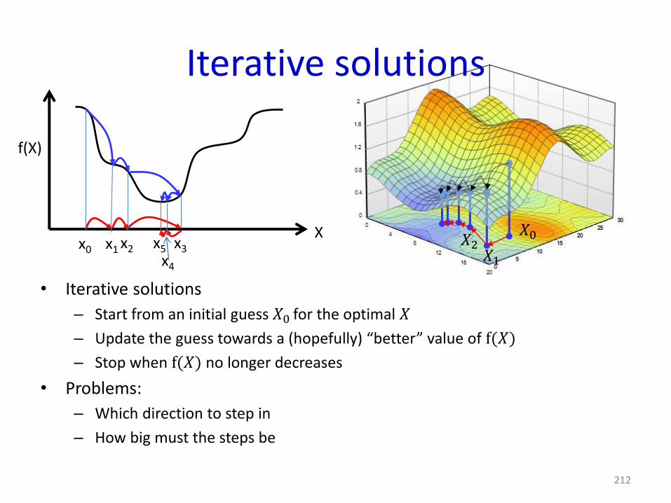
Iterative solutions
• Iterative solutions
– Start from an initial guess 𝑋0 for the optimal 𝑋
– Update the guess towards a (hopefully) “better” value of f(𝑋)
– Stop when f(𝑋) no longer decreases
• Problems:
– Which direction to step in
– How big must the steps be
212
f(X)
Xx0 x1 x2 x3
x4
x5
𝑋0
𝑋1𝑋2
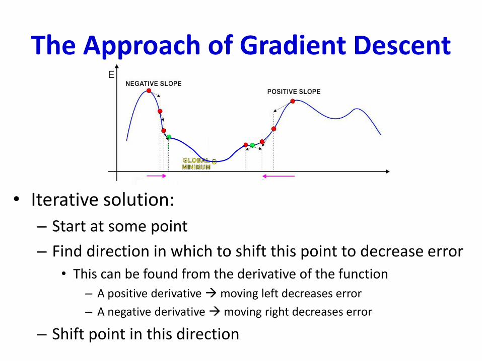
The Approach of Gradient Descent
• Iterative solution:
– Start at some point
– Find direction in which to shift this point to decrease error
• This can be found from the derivative of the function
– A positive derivative moving left decreases error
– A negative derivative moving right decreases error
– Shift point in this direction
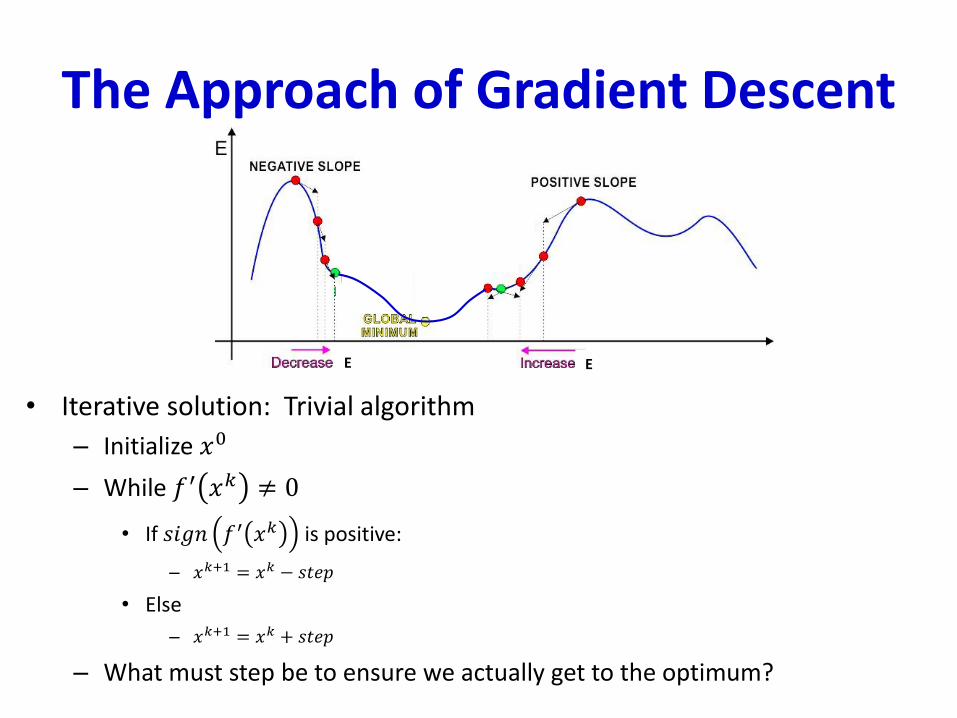
The Approach of Gradient Descent
• Iterative solution: Trivial algorithm
– Initialize 𝑥0
– While 𝑓′ 𝑥𝑘 ≠ 0
• If 𝑠𝑖𝑔𝑛 𝑓′ 𝑥𝑘 is positive:
– 𝑥𝑘+1 = 𝑥𝑘 − 𝑠𝑡𝑒𝑝
• Else
– 𝑥𝑘+1 = 𝑥𝑘 + 𝑠𝑡𝑒𝑝
– What must step be to ensure we actually get to the optimum?
E E
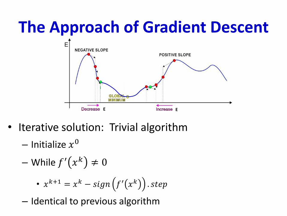
The Approach of Gradient Descent
• Iterative solution: Trivial algorithm
– Initialize 𝑥0
– While 𝑓′ 𝑥𝑘 ≠ 0
• 𝑥𝑘+1 = 𝑥𝑘 − 𝑠𝑖𝑔𝑛 𝑓′ 𝑥𝑘 . 𝑠𝑡𝑒𝑝
– Identical to previous algorithm
E E
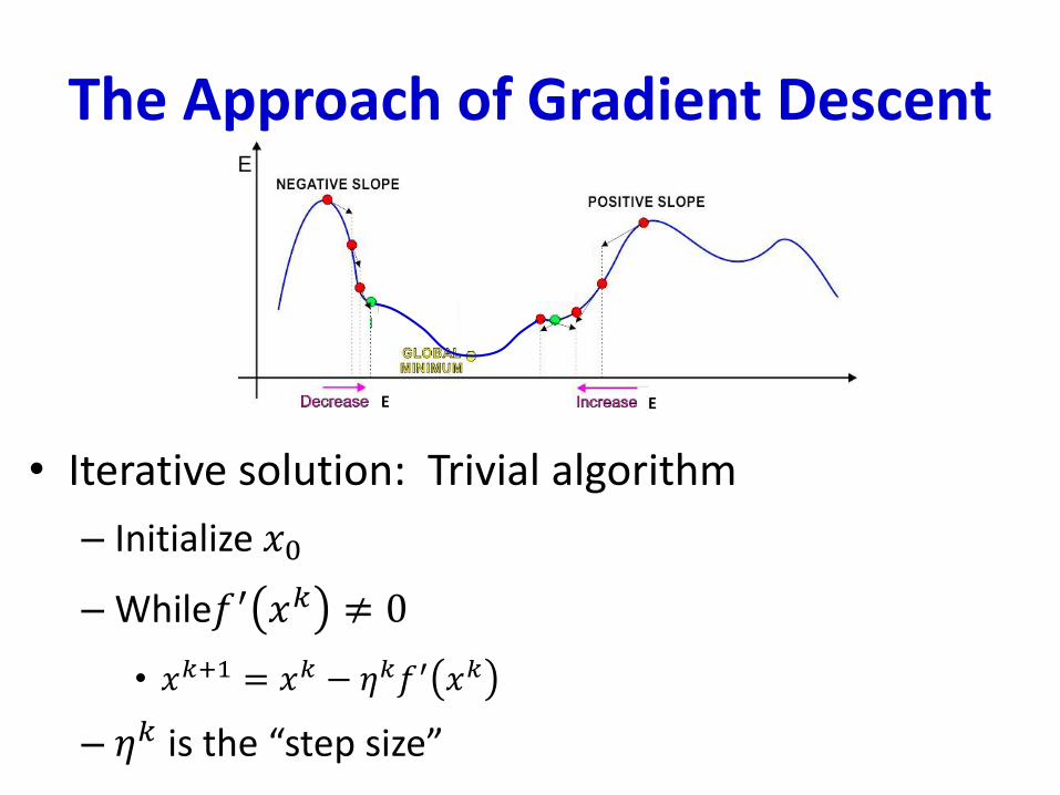
The Approach of Gradient Descent
• Iterative solution: Trivial algorithm
– Initialize 𝑥0
– While𝑓′ 𝑥𝑘 ≠ 0
• 𝑥𝑘+1 = 𝑥𝑘 − 𝜂𝑘𝑓′ 𝑥𝑘
– 𝜂𝑘 is the “step size”
E E
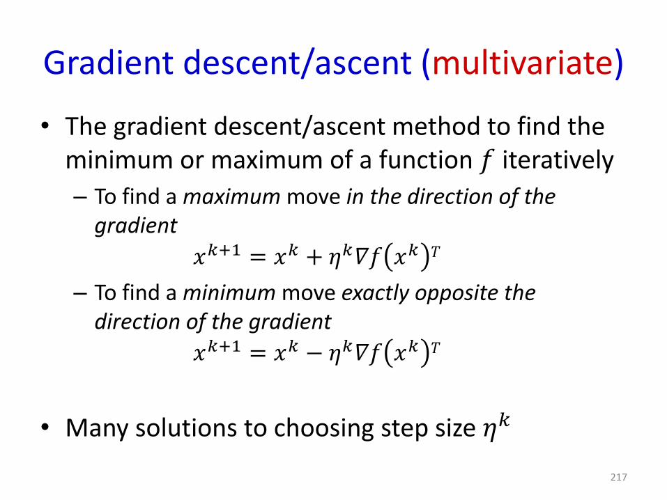
Gradient descent/ascent (multivariate)
• The gradient descent/ascent method to find the minimum or maximum of a function 𝑓 iteratively
– To find a maximum move in the direction of the gradient
𝑥𝑘+1 = 𝑥𝑘 + 𝜂𝑘𝛻𝑓 𝑥𝑘 𝑇
– To find a minimum move exactly opposite the direction of the gradient
𝑥𝑘+1 = 𝑥𝑘 − 𝜂𝑘𝛻𝑓 𝑥𝑘 𝑇
• Many solutions to choosing step size 𝜂𝑘
217
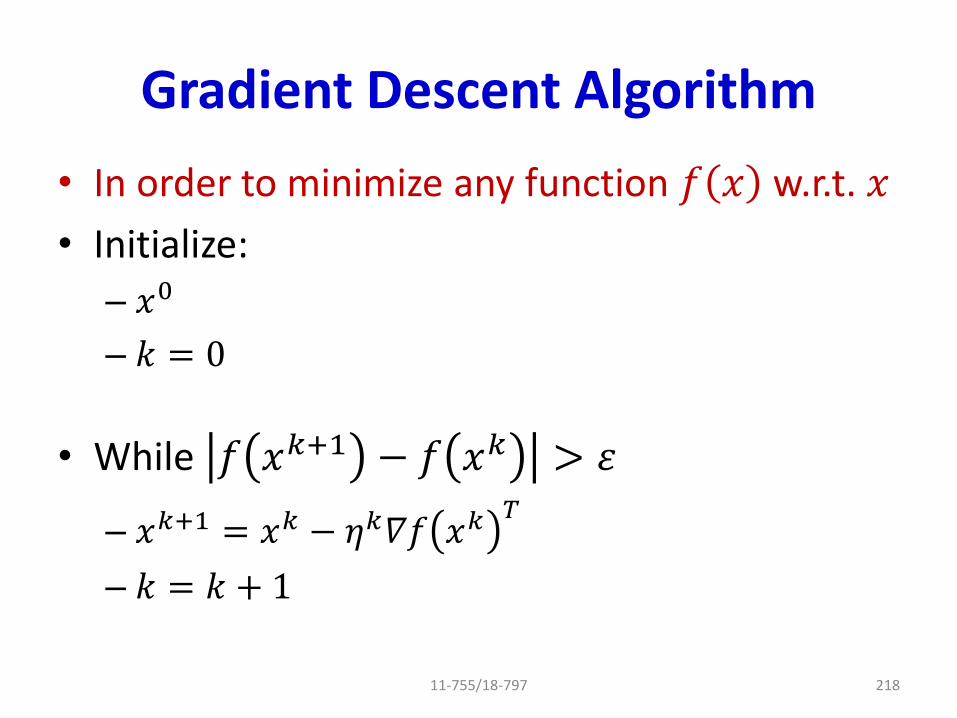
Gradient Descent Algorithm
• In order to minimize any function 𝑓 𝑥 w.r.t. 𝑥
• Initialize:
– 𝑥0
– 𝑘 = 0
• While 𝑓 𝑥𝑘+1 − 𝑓 𝑥𝑘 > 𝜀
– 𝑥𝑘+1 = 𝑥𝑘 − 𝜂𝑘𝛻𝑓 𝑥𝑘𝑇
– 𝑘 = 𝑘 + 1
11-755/18-797 218
• Back to Neural Networks
219
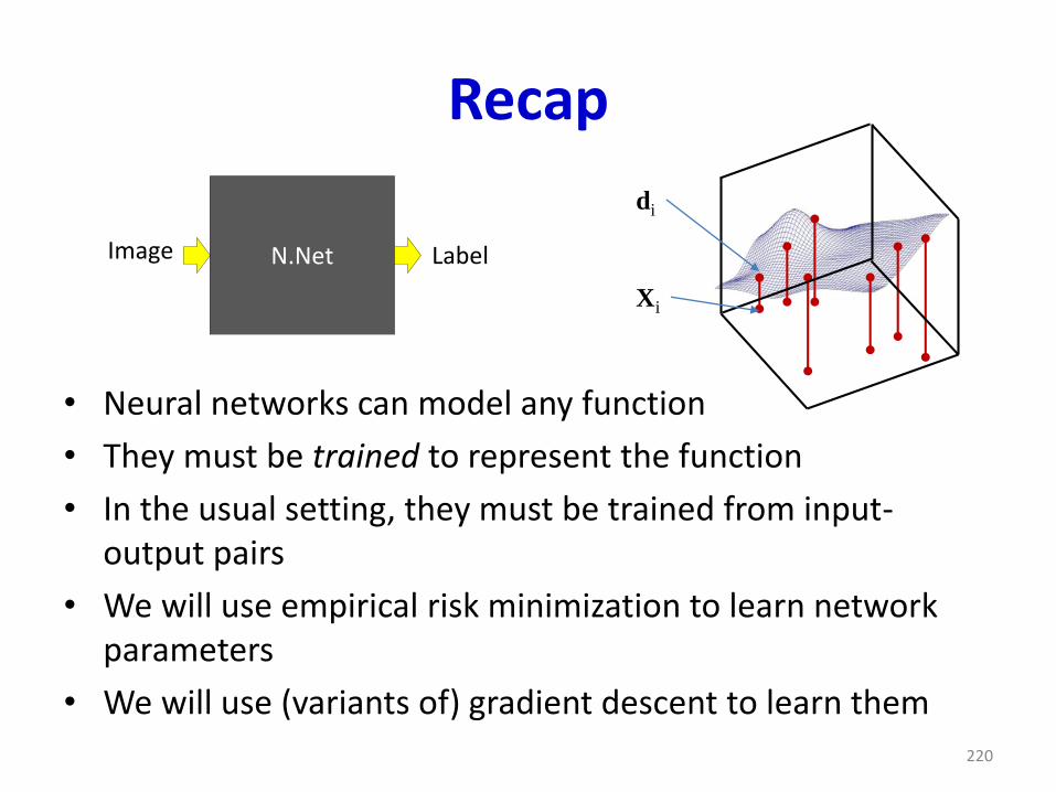
Recap
• Neural networks can model any function
• They must be trained to represent the function
• In the usual setting, they must be trained from input-output pairs
• We will use empirical risk minimization to learn network parameters
• We will use (variants of) gradient descent to learn them
220
N.NetImage Label
Xi
di
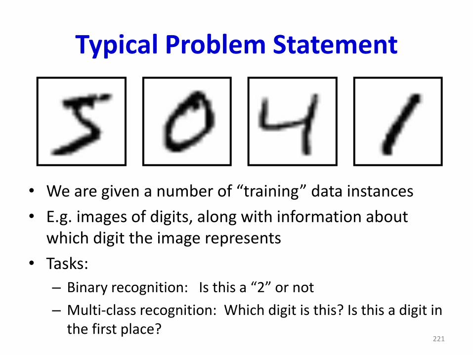
Typical Problem Statement
• We are given a number of “training” data instances
• E.g. images of digits, along with information about which digit the image represents
• Tasks:
– Binary recognition: Is this a “2” or not
– Multi-class recognition: Which digit is this? Is this a digit in the first place?
221
Representing the output
• If the desired output is real-valued, no special tricks are necessary
– Scalar Output : single output neuron• d = scalar (real value)
– Vector Output : as many output neurons as the dimension of the desired output• d = [d1 d2 .. dN] (vector of real values)
• If the desired output is binary (is this a cat or not), use a simple 1/0 output
– 1 = Yes it’s a cat
– 0 = No it’s not a cat.
• For multi-class outputs: one-hot representations
– For N classes, an N-dimensional binary vector of the form [0 0 0 1 0 0..]
– The single “1” in the k-th position represents an instance of the kth class
222
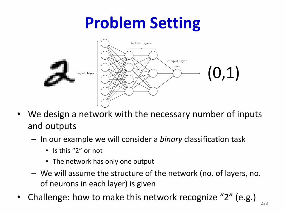
Problem Setting
• We design a network with the necessary number of inputs and outputs
– In our example we will consider a binary classification task
• Is this “2” or not
• The network has only one output
– We will assume the structure of the network (no. of layers, no. of neurons in each layer) is given
• Challenge: how to make this network recognize “2” (e.g.)223
(0,1)
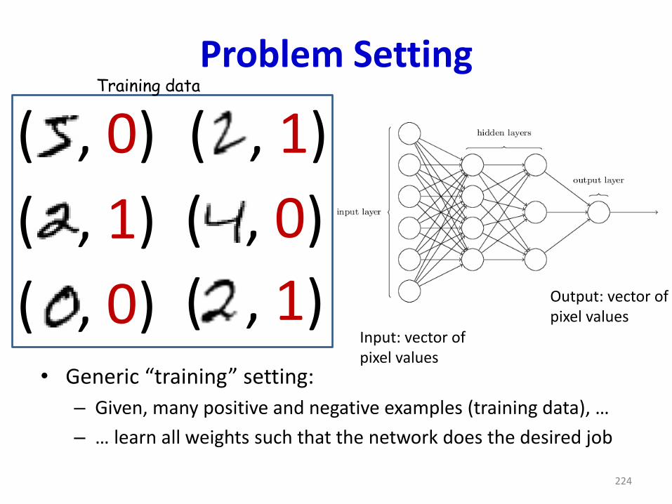
Problem Setting
• Generic “training” setting:
– Given, many positive and negative examples (training data), …
– … learn all weights such that the network does the desired job
224
( , 0)
( , 1)
( , 0)
( , 1)
( , 0)
( , 1)
Training data
Input: vector ofpixel values
Output: vector ofpixel values
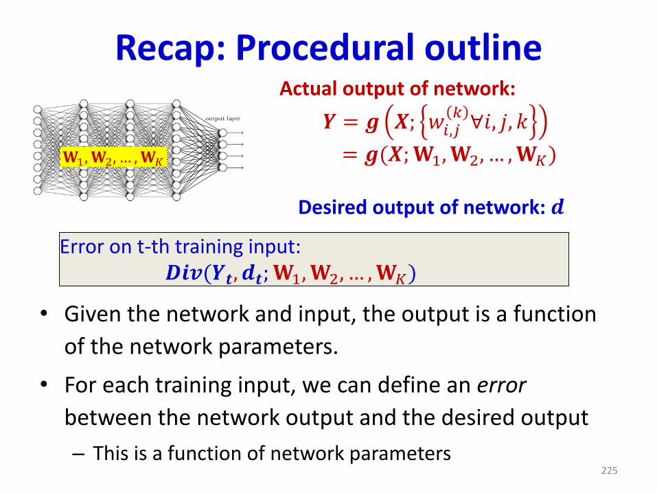
Recap: Procedural outline
• Given the network and input, the output is a function
of the network parameters.
• For each training input, we can define an error
between the network output and the desired output
– This is a function of network parameters
Actual output of network:
𝒀 = 𝒈 𝑿; 𝑤𝑖,𝑗𝑘∀𝑖, 𝑗, 𝑘
= 𝒈(𝑿;𝐖1,𝐖2, … ,𝐖𝐾)
Error on t-th training input:𝑫𝒊𝒗(𝒀𝒕, 𝒅𝒕;𝐖1,𝐖2, … ,𝐖𝐾)
𝐖1,𝐖2, … ,𝐖𝐾
225
Desired output of network: 𝒅
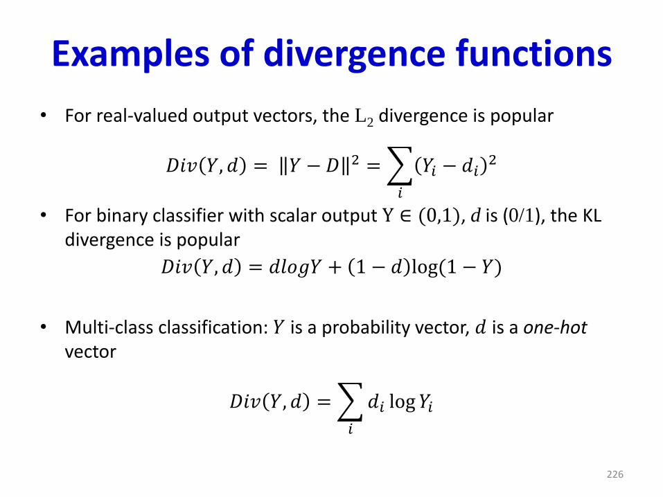
Examples of divergence functions
• For real-valued output vectors, the L2 divergence is popular
𝐷𝑖𝑣 𝑌, 𝑑 = 𝑌 − 𝐷 2 =
𝑖
𝑌𝑖 − 𝑑𝑖2
• For binary classifier with scalar output Y ∈ (0,1), d is (0/1), the KL divergence is popular
𝐷𝑖𝑣 𝑌, 𝑑 = 𝑑𝑙𝑜𝑔𝑌 + 1 − 𝑑 log(1 − 𝑌)
• Multi-class classification: 𝑌 is a probability vector, 𝑑 is a one-hot vector
𝐷𝑖𝑣 𝑌, 𝑑 =
𝑖
𝑑𝑖 log 𝑌𝑖
226
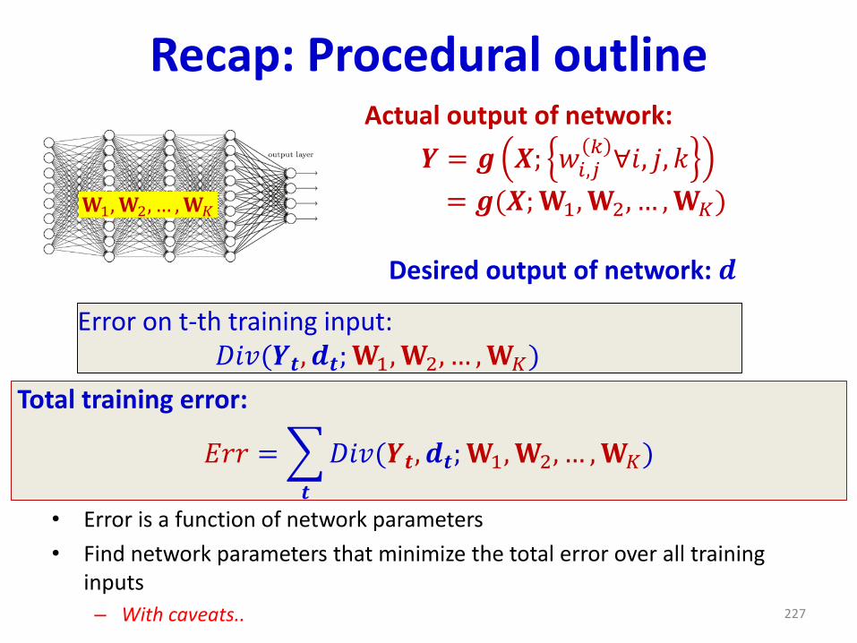
Recap: Procedural outline
• Error is a function of network parameters
• Find network parameters that minimize the total error over all training inputs
– With caveats..
Desired output of network: 𝒅
227
𝐖1,𝐖2, … ,𝐖𝐾
Total training error:
𝐸𝑟𝑟 =
𝒕
𝐷𝑖𝑣(𝒀𝒕, 𝒅𝒕;𝐖1,𝐖2, … ,𝐖𝐾)
Actual output of network:
𝒀 = 𝒈 𝑿; 𝑤𝑖,𝑗𝑘∀𝑖, 𝑗, 𝑘
= 𝒈(𝑿;𝐖1,𝐖2, … ,𝐖𝐾)
Error on t-th training input:𝐷𝑖𝑣(𝒀𝒕, 𝒅𝒕;𝐖1,𝐖2, … ,𝐖𝐾)
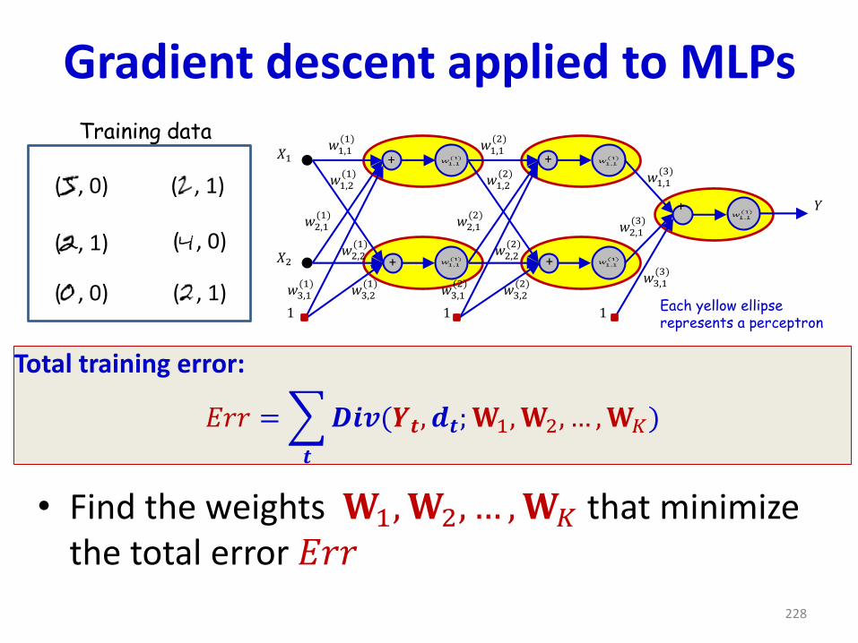
Gradient descent applied to MLPs
• Find the weights 𝐖1,𝐖2, … ,𝐖𝐾 that minimize the total error 𝐸𝑟𝑟
228
+
+
+
+
+
𝑋1
𝑋2
𝑌
1 1 1
𝑤1,1(1)
𝑤2,1(1)
𝑤3,1(1)
𝑤1,1(2)
𝑤2,1(2)
𝑤3,1(2)
𝑤1,1(3)
𝑤2,1(3)
𝑤3,1(3)
𝑤3,2(1)
𝑤3,2(2)
𝑤2,2(1)
𝑤1,2(1)
𝑤2,2(2)
𝑤1,2(2)
Each yellow ellipserepresents a perceptron
( , 0)
( , 1)
( , 0)
( , 1)
( , 0)
( , 1)
Training data
Total training error:
𝐸𝑟𝑟 =
𝒕
𝑫𝒊𝒗(𝒀𝒕, 𝒅𝒕;𝐖1,𝐖2, … ,𝐖𝐾)
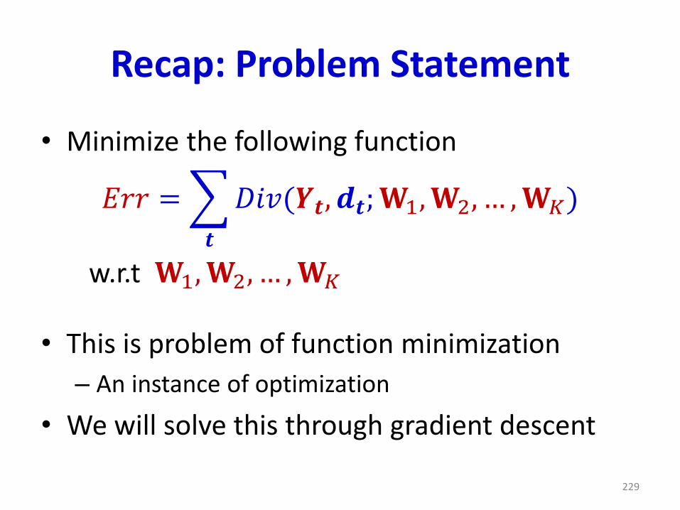
Recap: Problem Statement
• Minimize the following function
𝐸𝑟𝑟 =
𝒕
𝐷𝑖𝑣(𝒀𝒕, 𝒅𝒕;𝐖1,𝐖2, … ,𝐖𝐾)
w.r.t 𝐖1,𝐖2, … ,𝐖𝐾
• This is problem of function minimization
– An instance of optimization
• We will solve this through gradient descent
229
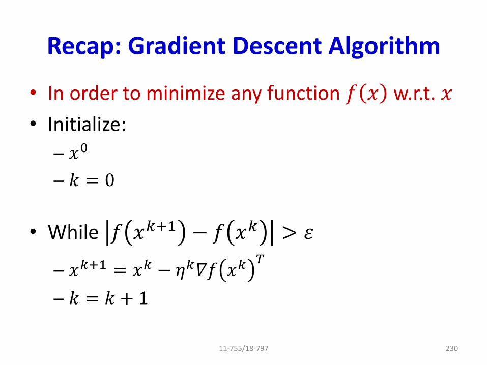
Recap: Gradient Descent Algorithm
• In order to minimize any function 𝑓 𝑥 w.r.t. 𝑥
• Initialize:
– 𝑥0
– 𝑘 = 0
• While 𝑓 𝑥𝑘+1 − 𝑓 𝑥𝑘 > 𝜀
– 𝑥𝑘+1 = 𝑥𝑘 − 𝜂𝑘𝛻𝑓 𝑥𝑘𝑇
– 𝑘 = 𝑘 + 1
11-755/18-797 230
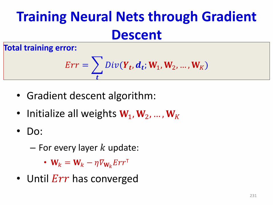
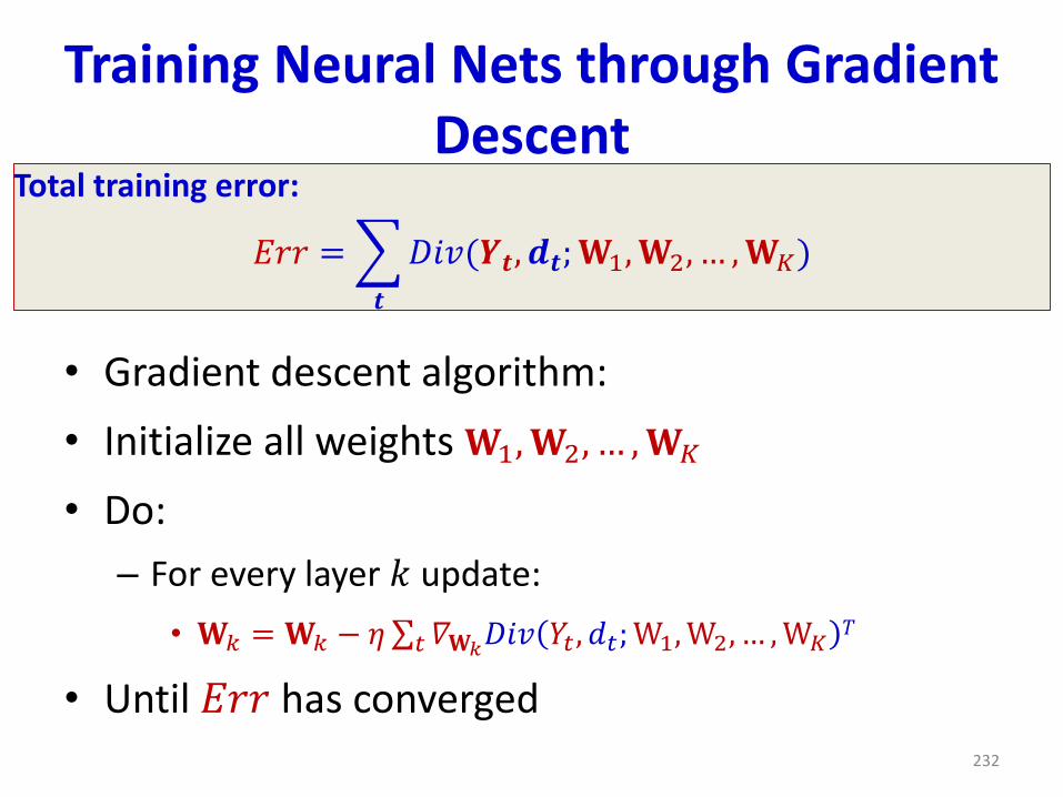
Training Neural Nets through Gradient Descent
• Gradient descent algorithm:
• Initialize all weights 𝐖1,𝐖2, … ,𝐖𝐾
• Do:
– For every layer 𝑘 update:
• 𝐖𝑘 = 𝐖𝑘 − 𝜂𝛻𝐖𝑘𝐸𝑟𝑟T
• Until 𝐸𝑟𝑟 has converged
231
Total training error:
𝐸𝑟𝑟 =
𝒕
𝐷𝑖𝑣(𝒀𝒕, 𝒅𝒕;𝐖1,𝐖2, … ,𝐖𝐾)
Training Neural Nets through Gradient Descent
• Gradient descent algorithm:
• Initialize all weights 𝐖1,𝐖2, … ,𝐖𝐾
• Do:
– For every layer 𝑘 update:
• 𝐖𝑘 = 𝐖𝑘 − 𝜂σ𝑡 𝛻𝐖𝑘𝐷𝑖𝑣 𝑌𝑡 , 𝑑𝑡;W1,W2, … ,W𝐾
𝑇
• Until 𝐸𝑟𝑟 has converged232
Total training error:
𝐸𝑟𝑟 =
𝒕
𝐷𝑖𝑣(𝒀𝒕, 𝒅𝒕;𝐖1,𝐖2, … ,𝐖𝐾)
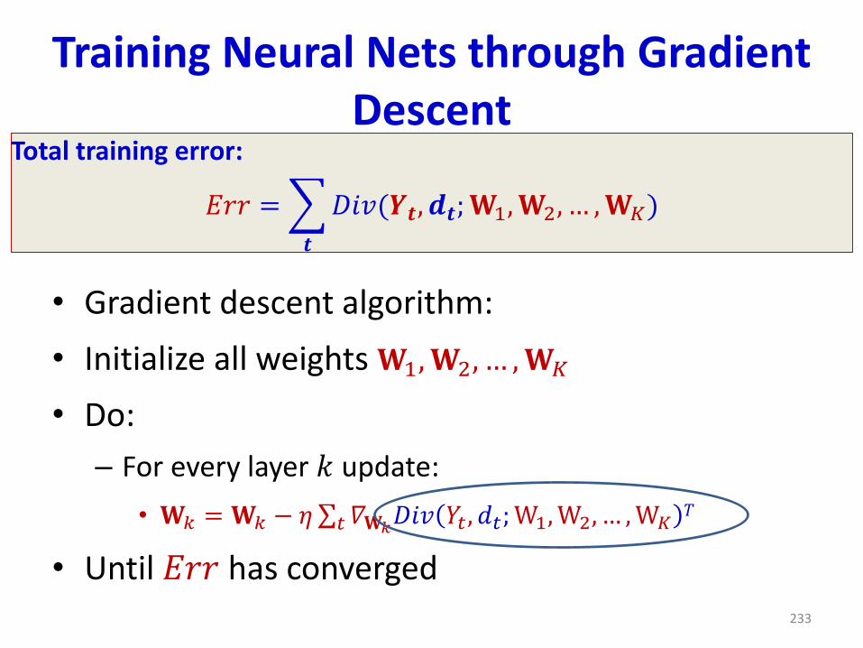
Training Neural Nets through Gradient Descent
• Gradient descent algorithm:
• Initialize all weights 𝐖1,𝐖2, … ,𝐖𝐾
• Do:
– For every layer 𝑘 update:
• 𝐖𝑘 = 𝐖𝑘 − 𝜂σ𝑡 𝛻𝐖𝑘𝐷𝑖𝑣 𝑌𝑡 , 𝑑𝑡;W1,W2, … ,W𝐾
𝑇
• Until 𝐸𝑟𝑟 has converged233
Total training error:
𝐸𝑟𝑟 =
𝒕
𝐷𝑖𝑣(𝒀𝒕, 𝒅𝒕;𝐖1,𝐖2, … ,𝐖𝐾)
Computing the derivatives
• We use back propagation to compute the derivative
• Assuming everyone knows how; will skip the details
Does backprop do the right thing?
• Is backprop always right?
– Assuming it actually find the global minimum of the divergence function?
• In classification problems, the classification error is a non-differentiable function of weights
• The divergence function minimized is only a proxy for classification error
• Minimizing divergence may not minimize classification error
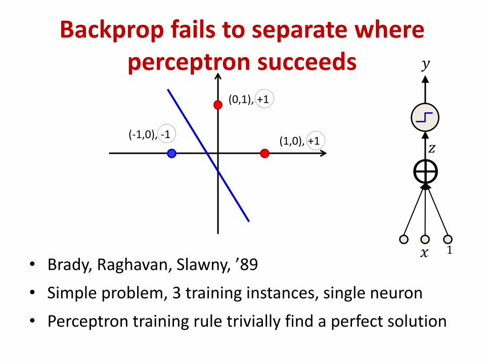
Backprop fails to separate where perceptron succeeds
• Brady, Raghavan, Slawny, ’89
• Simple problem, 3 training instances, single neuron
• Perceptron training rule trivially find a perfect solution
𝑥
𝑧
⨁
1
𝑦
(1,0), +1
(0,1), +1
(-1,0), -1
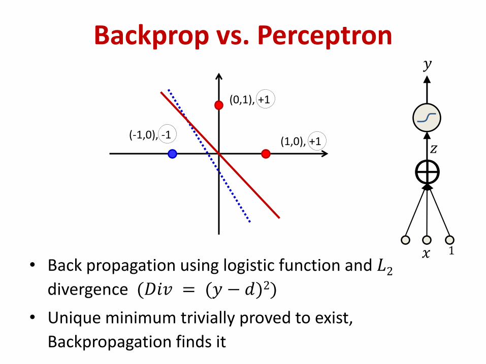
Backprop vs. Perceptron
• Back propagation using logistic function and 𝐿2divergence (𝐷𝑖𝑣 = (𝑦 − 𝑑)2)
• Unique minimum trivially proved to exist,
Backpropagation finds it
𝑥
𝑧
⨁
1
𝑦
(1,0), +1
(0,1), +1
(-1,0), -1
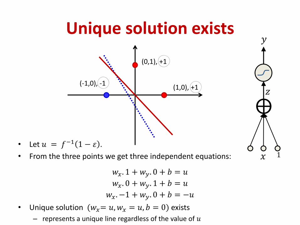
Unique solution exists
• Let 𝑢 = 𝑓−1 1 − 𝜀 .
• From the three points we get three independent equations:
𝑤𝑥 . 1 + 𝑤𝑦. 0 + 𝑏 = 𝑢
𝑤𝑥 . 0 + 𝑤𝑦. 1 + 𝑏 = 𝑢
𝑤𝑥 . −1 + 𝑤𝑦. 0 + 𝑏 = −𝑢
• Unique solution (𝑤𝑥= 𝑢,𝑤𝑥 = 𝑢, 𝑏 = 0) exists
– represents a unique line regardless of the value of 𝑢
𝑥
𝑧
⨁
1
𝑦
(1,0), +1
(0,1), +1
(-1,0), -1
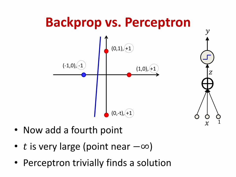
Backprop vs. Perceptron
• Now add a fourth point
• 𝑡 is very large (point near −∞)
• Perceptron trivially finds a solution
𝑥
𝑧
⨁
1
𝑦
(1,0), +1
(0,1), +1
(-1,0), -1
(0,-t), +1
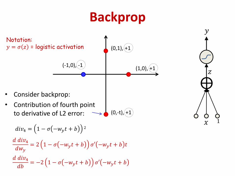
Backprop
• Consider backprop:
• Contribution of fourth point to derivative of L2 error:
𝑥
𝑧
⨁
1
𝑦
(1,0), +1
(0,1), +1
(-1,0), -1
(0,-t), +1
𝑑𝑖𝑣4 = 1 − 𝜎 −𝑤𝑦𝑡 + 𝑏 2
Notation:𝑦 = 𝜎 𝑧 = logistic activation
𝑑 𝑑𝑖𝑣4𝑑𝑤𝑦
= 2 1 − 𝜎 −𝑤𝑦𝑡 + 𝑏 𝜎′ −𝑤𝑦𝑡 + 𝑏 𝑡
𝑑 𝑑𝑖𝑣4𝑑𝑏
= −2 1 − 𝜎 −𝑤𝑦𝑡 + 𝑏 𝜎′ −𝑤𝑦𝑡 + 𝑏
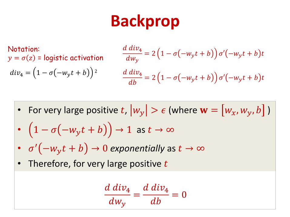
Backprop
𝑑𝑖𝑣4 = 1 − 𝜎 −𝑤𝑦𝑡 + 𝑏 2
Notation:𝑦 = 𝜎 𝑧 = logistic activation
𝑑 𝑑𝑖𝑣4𝑑𝑤𝑦
= 2 1 − 𝜎 −𝑤𝑦𝑡 + 𝑏 𝜎′ −𝑤𝑦𝑡 + 𝑏 𝑡
𝑑 𝑑𝑖𝑣4𝑑𝑏
= 2 1 − 𝜎 −𝑤𝑦𝑡 + 𝑏 𝜎′ −𝑤𝑦𝑡 + 𝑏 𝑡
• For very large positive 𝑡, 𝑤𝑦 > 𝜖 (where 𝐰 = 𝑤𝑥 , 𝑤𝑦, 𝑏 )
• 1 − 𝜎 −𝑤𝑦𝑡 + 𝑏 → 1 as 𝑡 → ∞
• 𝜎′ −𝑤𝑦𝑡 + 𝑏 → 0 exponentially as 𝑡 → ∞
• Therefore, for very large positive 𝑡
𝑑 𝑑𝑖𝑣4𝑑𝑤𝑦
=𝑑 𝑑𝑖𝑣4𝑑𝑏
= 0
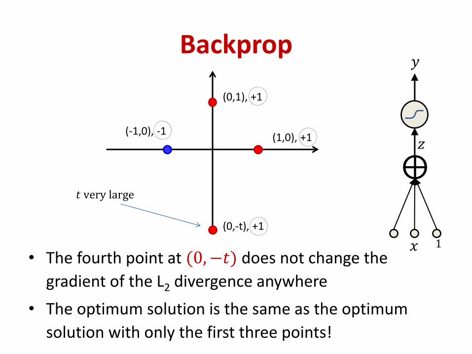
Backprop
• The fourth point at (0, −𝑡) does not change the
gradient of the L2 divergence anywhere
• The optimum solution is the same as the optimum
solution with only the first three points!
𝑥
𝑧
⨁
1
𝑦
(1,0), +1
(0,1), +1
(-1,0), -1
(0,-t), +1
𝑡 very large
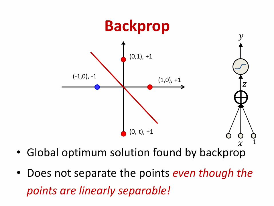
Backprop
• Global optimum solution found by backprop
• Does not separate the points even though the
points are linearly separable!
𝑥
𝑧
⨁
1
𝑦
(1,0), +1
(0,1), +1
(-1,0), -1
(0,-t), +1
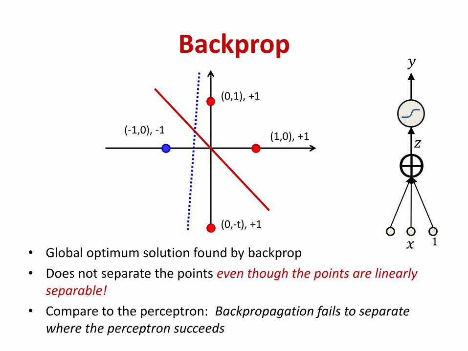
Backprop
• Global optimum solution found by backprop
• Does not separate the points even though the points are linearly separable!
• Compare to the perceptron: Backpropagation fails to separate where the perceptron succeeds
𝑥
𝑧
⨁
1
𝑦
(1,0), +1
(0,1), +1
(-1,0), -1
(0,-t), +1
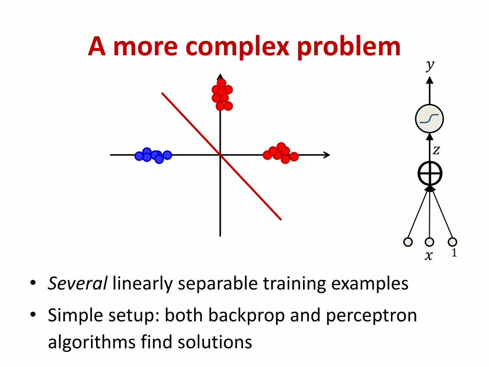
A more complex problem
• Several linearly separable training examples
• Simple setup: both backprop and perceptron
algorithms find solutions
𝑥
𝑧
⨁
1
𝑦

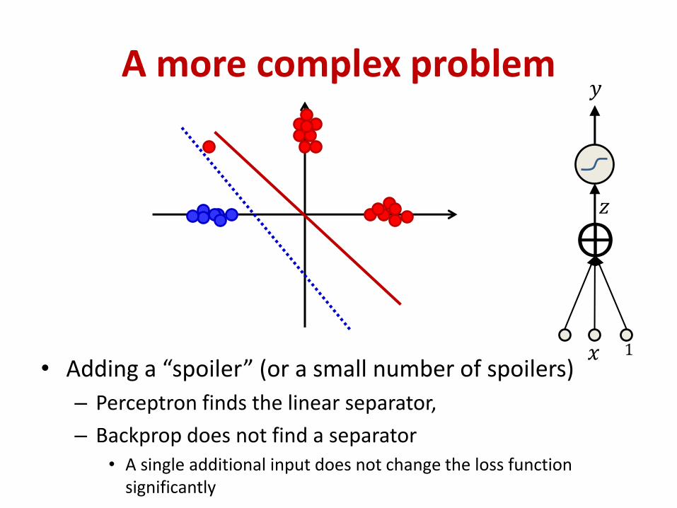
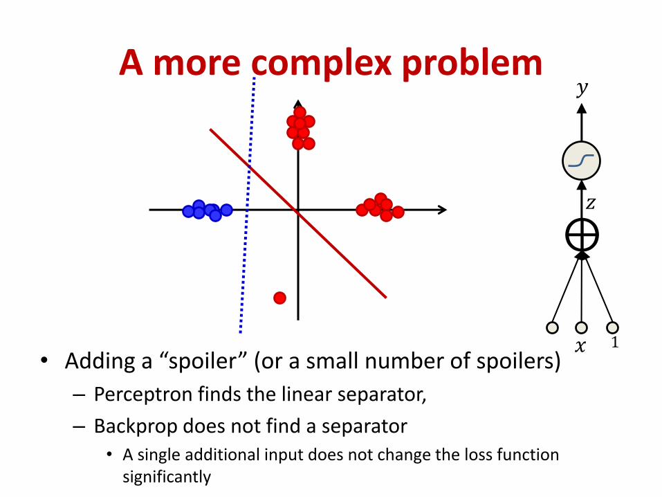
A more complex problem
• Adding a “spoiler” (or a small number of spoilers)
– Perceptron finds the linear separator,
– Backprop does not find a separator• A single additional input does not change the loss function
significantly
𝑥
𝑧
⨁
1
𝑦
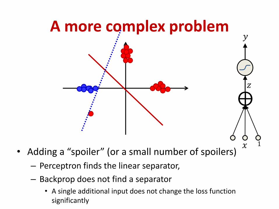
A more complex problem
𝑥
𝑧
⨁
1
𝑦
• Adding a “spoiler” (or a small number of spoilers)
– Perceptron finds the linear separator,
– Backprop does not find a separator• A single additional input does not change the loss function
significantly
A more complex problem
𝑥
𝑧
⨁
1
𝑦
• Adding a “spoiler” (or a small number of spoilers)
– Perceptron finds the linear separator,
– Backprop does not find a separator• A single additional input does not change the loss function
significantly
A more complex problem
𝑥
𝑧
⨁
1
𝑦
• Adding a “spoiler” (or a small number of spoilers)
– Perceptron finds the linear separator,
– Backprop does not find a separator• A single additional input does not change the loss function
significantly
So what is happening here?
• The perceptron may change greatly upon adding just a single new training instance
– But it fits the training data well
– The perceptron rule has low bias • Makes no errors if possible
– But high variance• Swings wildly in response to small changes to input
• Backprop is minimally changed by new training instances
– Prefers consistency over perfection
– It is a low-variance estimator, at the potential cost of bias
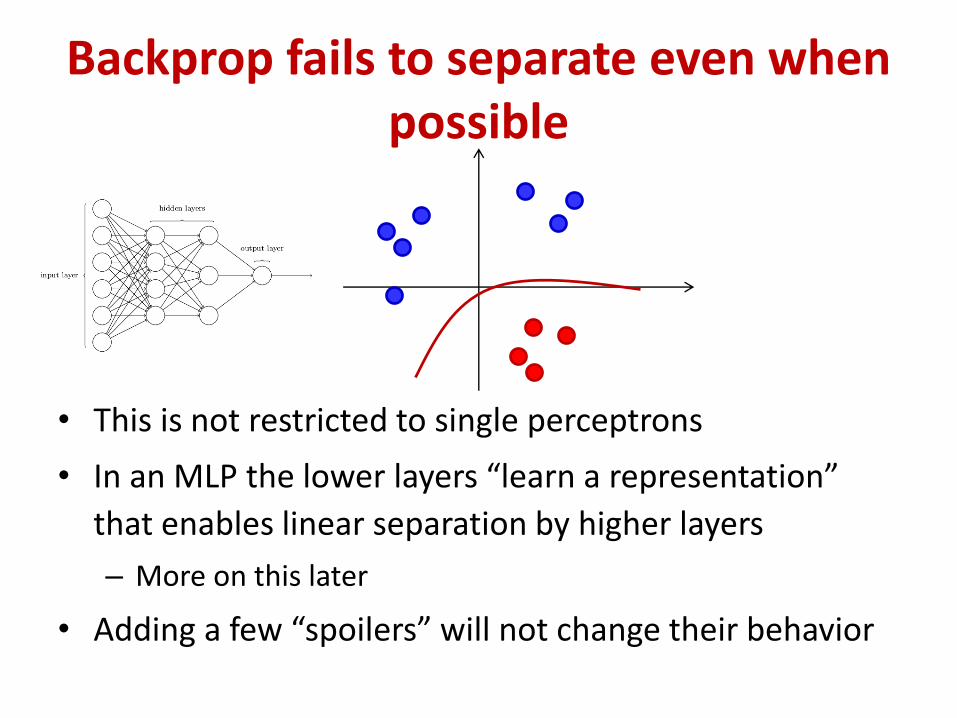
Backprop fails to separate even when possible
• This is not restricted to single perceptrons
• In an MLP the lower layers “learn a representation”
that enables linear separation by higher layers
• Adding a few “spoilers” will not change their behavior
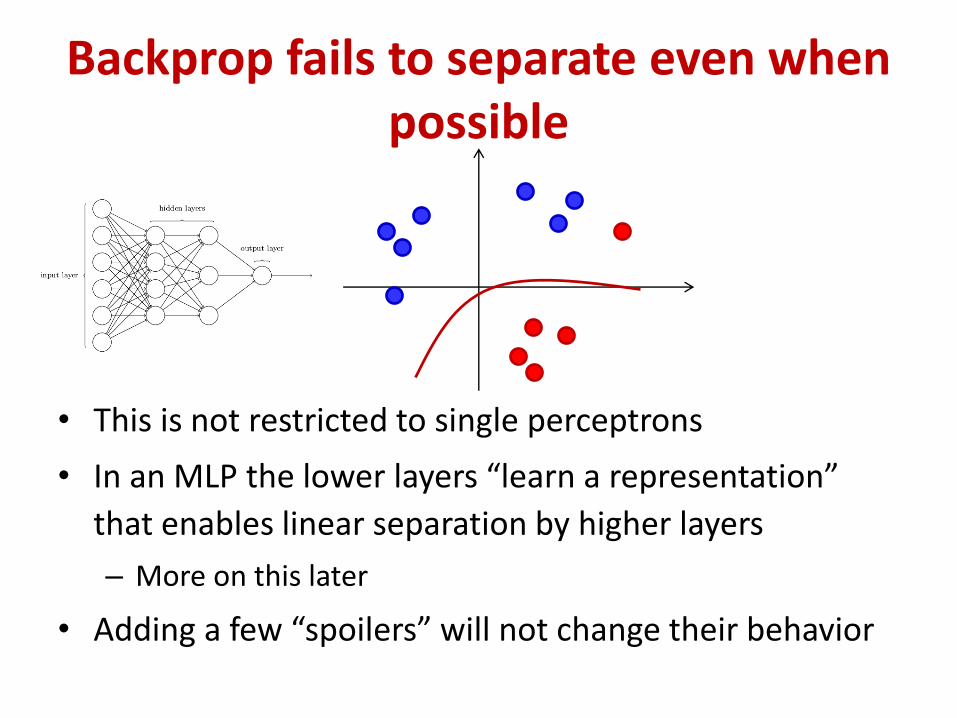
Backprop fails to separate even when possible
• This is not restricted to single perceptrons
• In an MLP the lower layers “learn a representation”
that enables linear separation by higher layers
• Adding a few “spoilers” will not change their behavior
Backpropagation
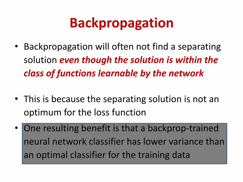
• Backpropagation will often not find a separating
solution even though the solution is within the
class of functions learnable by the network
• This is because the separating solution is not an
optimum for the loss function
• One resulting benefit is that a backprop-trained
neural network classifier has lower variance than
an optimal classifier for the training data
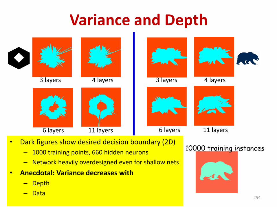
Variance and Depth
• Dark figures show desired decision boundary (2D)
– 1000 training points, 660 hidden neurons
– Network heavily overdesigned even for shallow nets
• Anecdotal: Variance decreases with
– Depth
– Data254
6 layers 11 layers
3 layers 4 layers
6 layers 11 layers
3 layers 4 layers
10000 training instances
Convergence
• How fast does it converge?
– And where?
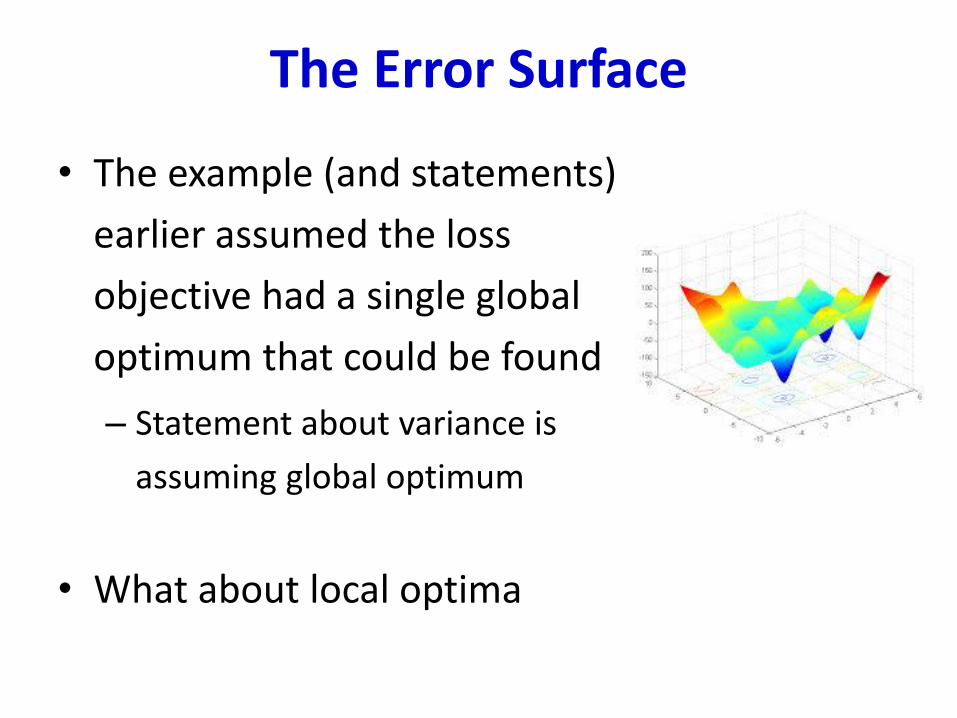
The Error Surface
• The example (and statements)
earlier assumed the loss
objective had a single global
optimum that could be found
– Statement about variance is
assuming global optimum
• What about local optima
The Error Surface
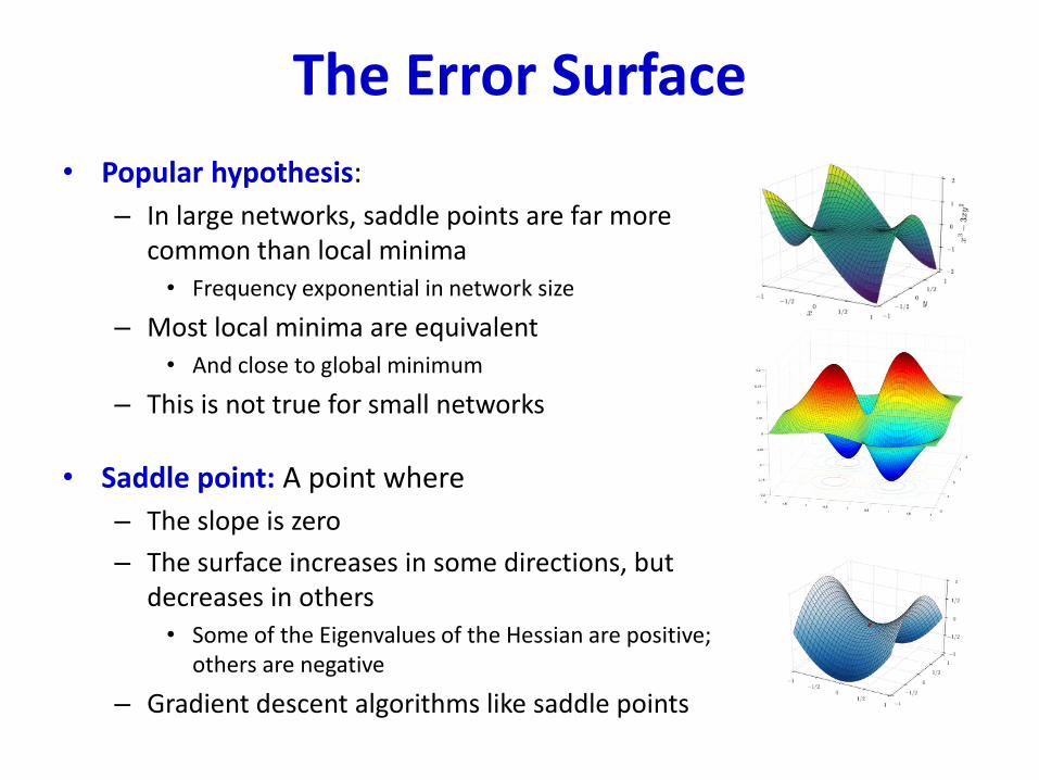
• Popular hypothesis:
– In large networks, saddle points are far more common than local minima
• Frequency exponential in network size
– Most local minima are equivalent
• And close to global minimum
– This is not true for small networks
• Saddle point: A point where
– The slope is zero
– The surface increases in some directions, but decreases in others
• Some of the Eigenvalues of the Hessian are positive; others are negative
– Gradient descent algorithms like saddle points
The Controversial Error Surface
• Baldi and Hornik (89), “Neural Networks and Principal Component Analysis: Learning from Examples Without Local Minima” : An MLP with a single hidden layer has only saddle points and no local Minima
• Dauphin et. al (2015), “Identifying and attacking the saddle point problem in high-dimensional non-convex optimization” : An exponential number of saddle points in large networks
• Chomoranksa et. al (2015), “The loss surface of multilayer networks” : For large networks, most local minima lie in a band and are equivalent
– Based on analysis of spin glass models
• Swirscz et. al. (2016), “Local minima in training of deep networks”, In networks of finite size, trained on finite data, you can have horrible local minima
• Watch this space…
Story so far
• Neural nets can be trained via gradient descent that minimizes a loss function
• Backpropagation can be used to derive the derivatives of the loss
• Backprop is not guaranteed to find a “true” solution, even if it exists, and lies within the capacity of the network to model
– The optimum for the loss function may not be the “true” solution
• For large networks, the loss function may have a large number of unpleasant saddle points
– Which backpropagation may find
Convergence
• In the discussion so far we have assumed the training arrives at a local minimum
• Does it always converge?
• How long does it take?
• Hard to analyze for an MLP, so lets look at convex optimization instead

A quick tour of (convex) optimization
Convex Loss Functions
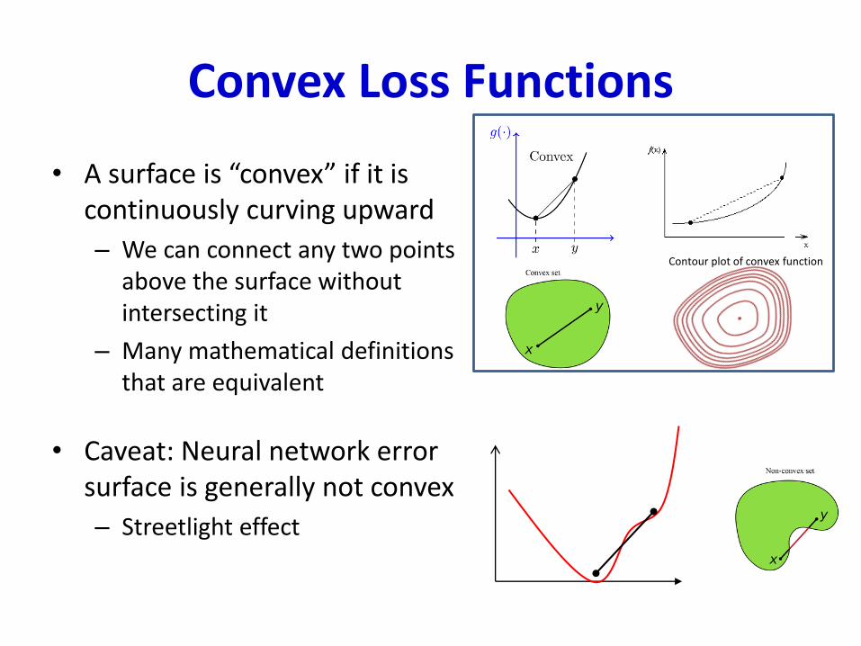
• A surface is “convex” if it is continuously curving upward
– We can connect any two points above the surface without intersecting it
– Many mathematical definitions that are equivalent
• Caveat: Neural network error surface is generally not convex
– Streetlight effect
Contour plot of convex function
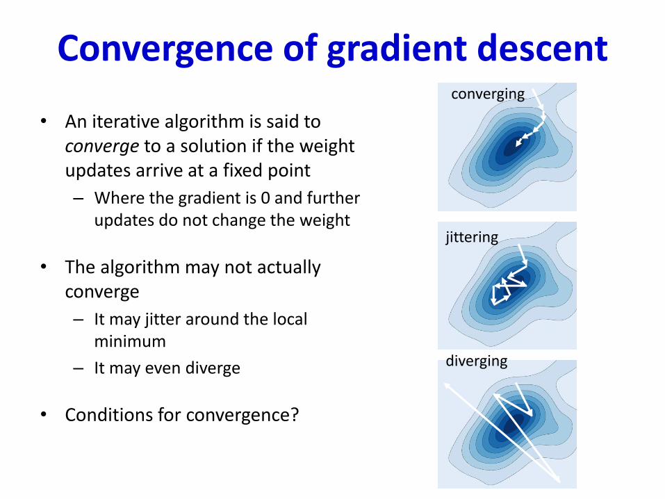
Convergence of gradient descent
• An iterative algorithm is said to converge to a solution if the weight updates arrive at a fixed point
– Where the gradient is 0 and further updates do not change the weight
• The algorithm may not actually converge
– It may jitter around the local minimum
– It may even diverge
• Conditions for convergence?
converging
jittering
diverging
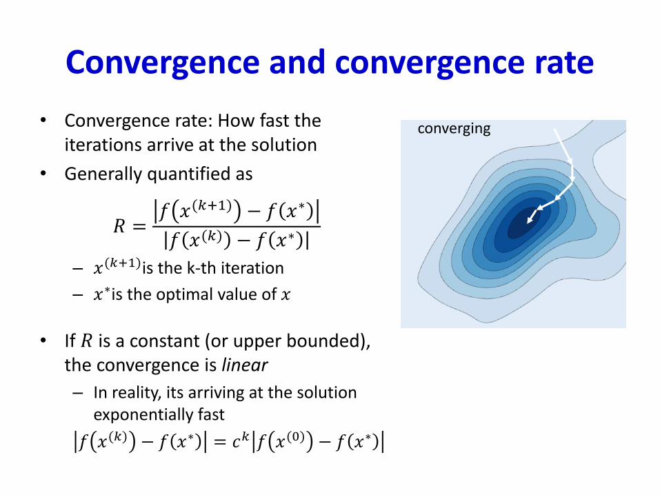
Convergence and convergence rate
• Convergence rate: How fast the iterations arrive at the solution
• Generally quantified as
𝑅 =𝑓 𝑥(𝑘+1) − 𝑓 𝑥∗
𝑓 𝑥(𝑘) − 𝑓 𝑥∗
– 𝑥(𝑘+1)is the k-th iteration
– 𝑥∗is the optimal value of 𝑥
• If 𝑅 is a constant (or upper bounded), the convergence is linear
– In reality, its arriving at the solution exponentially fast
𝑓 𝑥(𝑘) − 𝑓 𝑥∗ = 𝑐𝑘 𝑓 𝑥(0) − 𝑓 𝑥∗
converging
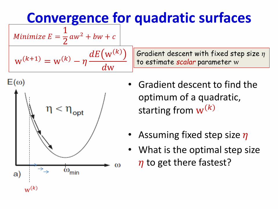
Convergence for quadratic surfaces
• Gradient descent to find the optimum of a quadratic,
starting from w(𝑘)
• Assuming fixed step size 𝜂
• What is the optimal step size 𝜂 to get there fastest?
w(𝑘+1) = w(𝑘) − 𝜂𝑑𝐸 w(𝑘)
𝑑w
Gradient descent with fixed step size 𝜂to estimate scalar parameter w
w(𝑘)
𝑀𝑖𝑛𝑖𝑚𝑖𝑧𝑒 𝐸 =12𝑎𝑤2 + 𝑏𝑤 + 𝑐
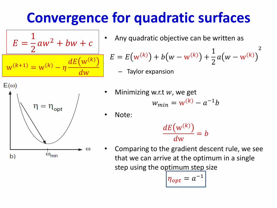
Convergence for quadratic surfaces• Any quadratic objective can be written as
𝐸 = 𝐸 w(𝑘) + 𝑏 𝑤 −w(𝑘) +1
2𝑎 𝑤 − w(𝑘)
2
– Taylor expansion
• Minimizing w.r.t 𝑤, we get
𝑤𝑚𝑖𝑛 = w(𝑘) − 𝑎−1𝑏
• Note:
𝑑𝐸 w(𝑘)
𝑑w= 𝑏
• Comparing to the gradient descent rule, we see that we can arrive at the optimum in a single step using the optimum step size
𝜂𝑜𝑝𝑡 = 𝑎−1
w(𝑘+1) = w(𝑘) − 𝜂𝑑𝐸 w(𝑘)
𝑑w
𝐸 =1
2𝑎𝑤2 + 𝑏𝑤 + 𝑐
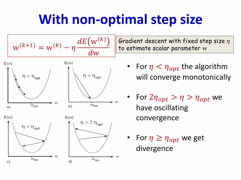
With non-optimal step size
• For 𝜂 < 𝜂𝑜𝑝𝑡 the algorithm
will converge monotonically
• For 2𝜂𝑜𝑝𝑡 > 𝜂 > 𝜂𝑜𝑝𝑡 we
have oscillating convergence
• For 𝜂 ≥ 𝜂𝑜𝑝𝑡 we get
divergence
w(𝑘+1) = w(𝑘) − 𝜂𝑑𝐸 w(𝑘)
𝑑w
Gradient descent with fixed step size 𝜂to estimate scalar parameter w
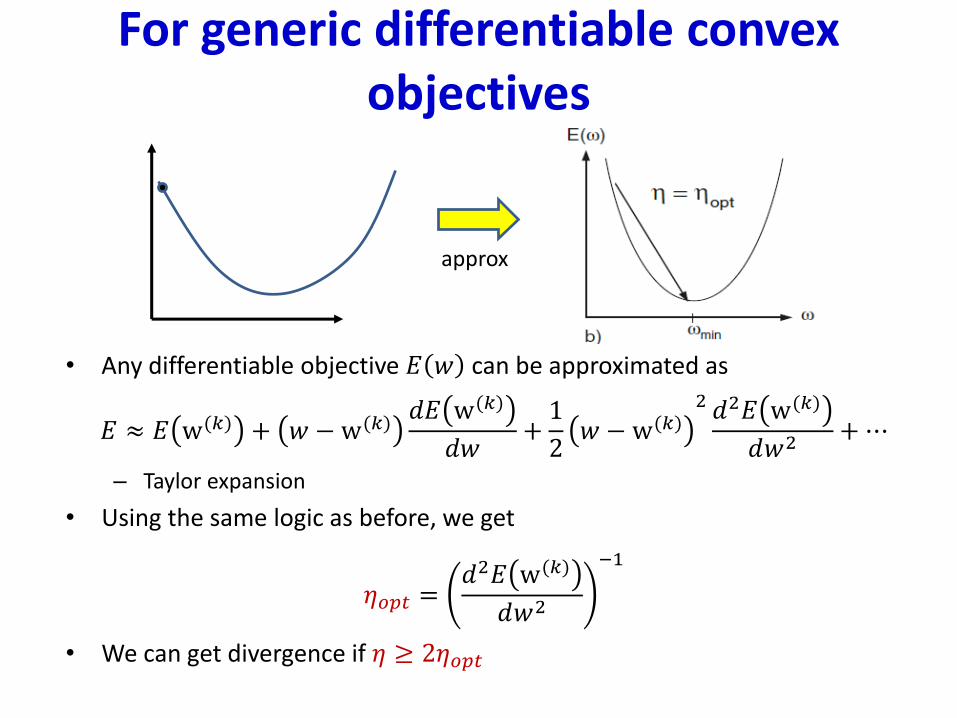
For generic differentiable convex objectives
• Any differentiable objective 𝐸 𝑤 can be approximated as
𝐸 ≈ 𝐸 w(𝑘) + 𝑤 −w(𝑘)𝑑𝐸 w(𝑘)
𝑑𝑤+1
2𝑤 − w(𝑘)
2 𝑑2𝐸 w(𝑘)
𝑑𝑤2+⋯
– Taylor expansion
• Using the same logic as before, we get
𝜂𝑜𝑝𝑡 =𝑑2𝐸 w(𝑘)
𝑑𝑤2
−1
• We can get divergence if 𝜂 ≥ 2𝜂𝑜𝑝𝑡
approx
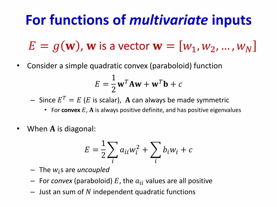
For functions of multivariate inputs
• Consider a simple quadratic convex (paraboloid) function
𝐸 =1
2𝐰𝑇𝐀𝐰+𝐰𝑇𝐛 + 𝑐
– Since 𝐸𝑇 = 𝐸 (𝐸 is scalar), 𝐀 can always be made symmetric
• For convex 𝐸, 𝐀 is always positive definite, and has positive eigenvalues
• When 𝐀 is diagonal:
𝐸 =1
2
𝑖
𝑎𝑖𝑖𝑤𝑖2 +
𝑖
𝑏𝑖𝑤𝑖 + 𝑐
– The 𝑤𝑖s are uncoupled
– For convex (paraboloid) 𝐸, the 𝑎𝑖𝑖 values are all positive
– Just an sum of 𝑁 independent quadratic functions
𝐸 = 𝑔 𝐰 , 𝐰 is a vector 𝐰 = 𝑤1, 𝑤2, … , 𝑤𝑁
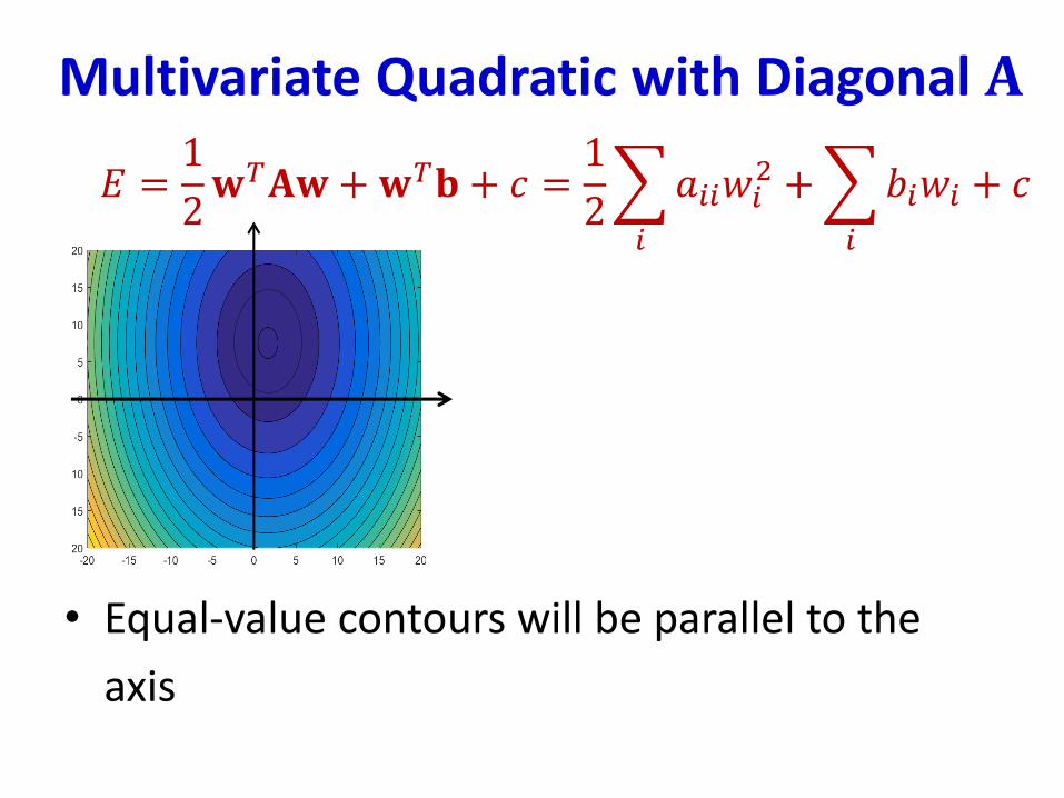
Multivariate Quadratic with Diagonal 𝐀
• Equal-value contours will be parallel to the
axis
𝐸 =1
2𝐰𝑇𝐀𝐰 +𝐰𝑇𝐛 + 𝑐 =
1
2
𝑖
𝑎𝑖𝑖𝑤𝑖2 +
𝑖
𝑏𝑖𝑤𝑖 + 𝑐
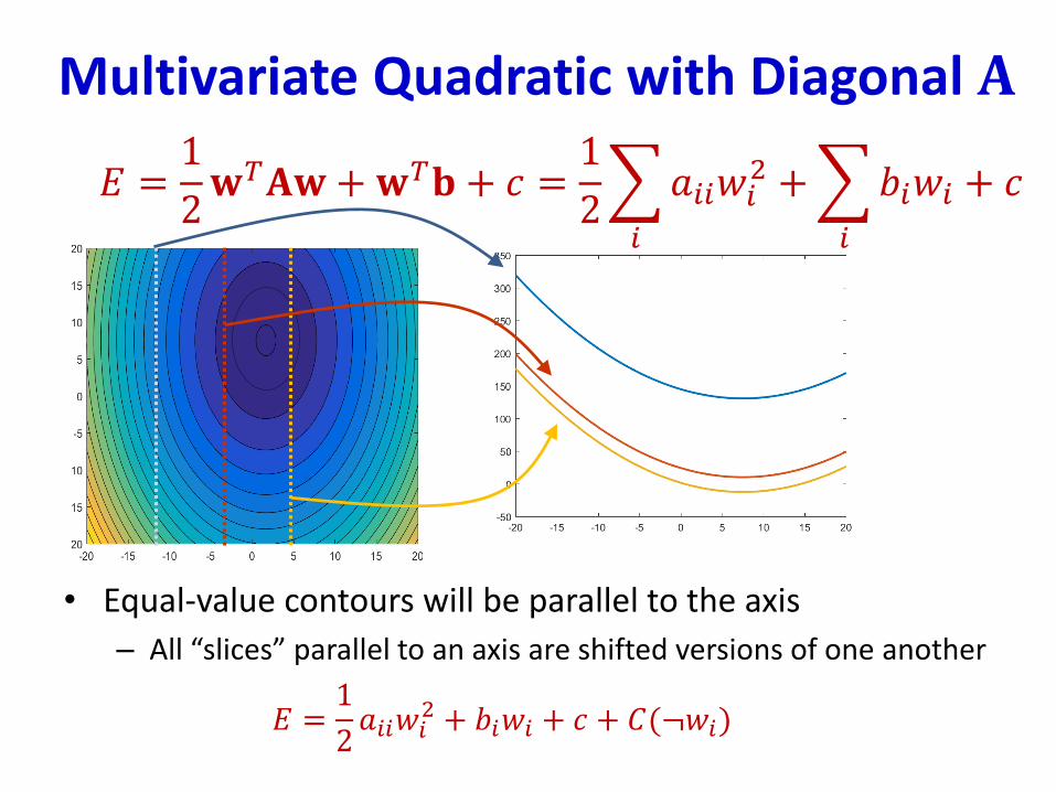
Multivariate Quadratic with Diagonal 𝐀
• Equal-value contours will be parallel to the axis
– All “slices” parallel to an axis are shifted versions of one another
𝐸 =1
2𝑎𝑖𝑖𝑤𝑖
2 + 𝑏𝑖𝑤𝑖 + 𝑐 + 𝐶(¬𝑤𝑖)
𝐸 =1
2𝐰𝑇𝐀𝐰 +𝐰𝑇𝐛 + 𝑐 =
1
2
𝑖
𝑎𝑖𝑖𝑤𝑖2 +
𝑖
𝑏𝑖𝑤𝑖 + 𝑐
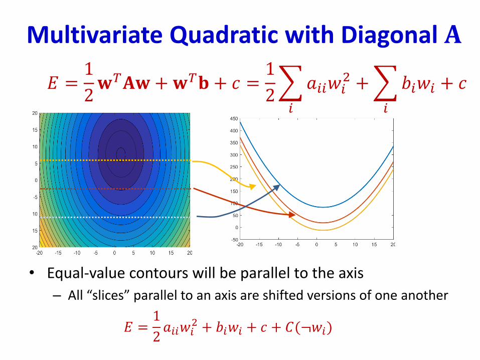
Multivariate Quadratic with Diagonal 𝐀
𝐸 =1
2𝐰𝑇𝐀𝐰 +𝐰𝑇𝐛 + 𝑐 =
1
2
𝑖
𝑎𝑖𝑖𝑤𝑖2 +
𝑖
𝑏𝑖𝑤𝑖 + 𝑐
• Equal-value contours will be parallel to the axis
– All “slices” parallel to an axis are shifted versions of one another
𝐸 =1
2𝑎𝑖𝑖𝑤𝑖
2 + 𝑏𝑖𝑤𝑖 + 𝑐 + 𝐶(¬𝑤𝑖)
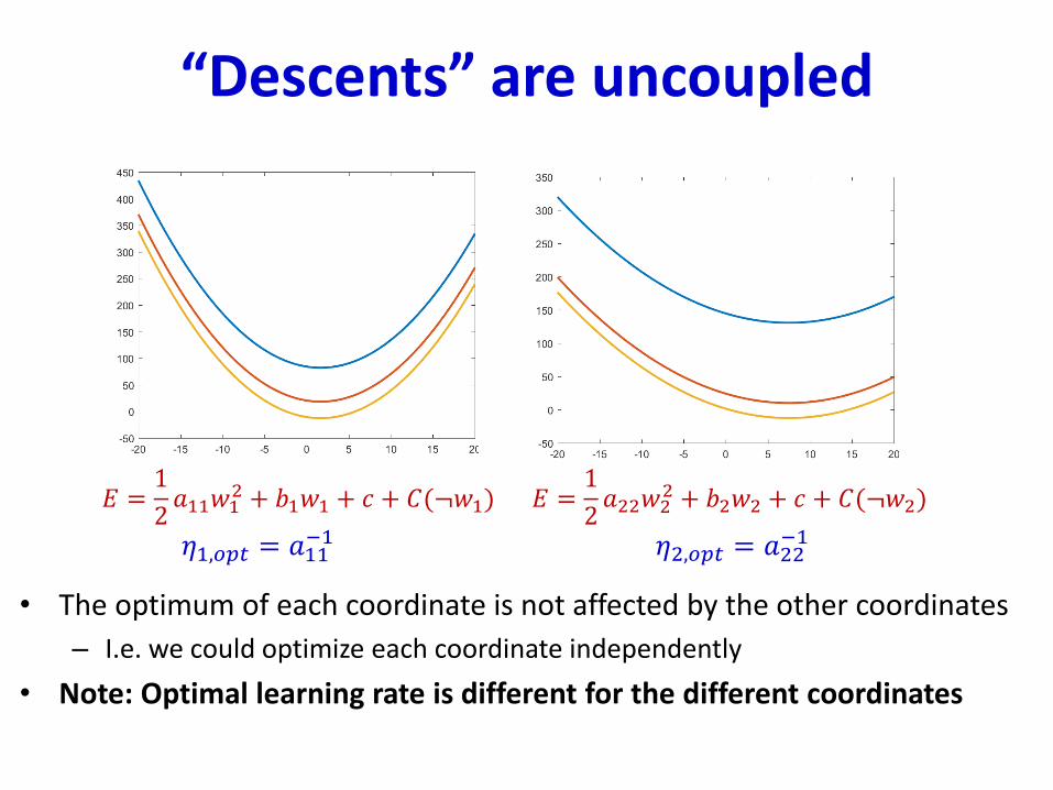
“Descents” are uncoupled
• The optimum of each coordinate is not affected by the other coordinates
– I.e. we could optimize each coordinate independently
• Note: Optimal learning rate is different for the different coordinates
𝐸 =1
2𝑎11𝑤1
2 + 𝑏1𝑤1 + 𝑐 + 𝐶(¬𝑤1) 𝐸 =1
2𝑎22𝑤2
2 + 𝑏2𝑤2 + 𝑐 + 𝐶(¬𝑤2)
𝜂1,𝑜𝑝𝑡 = 𝑎11−1 𝜂2,𝑜𝑝𝑡 = 𝑎22
−1
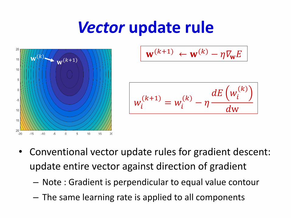
Vector update rule
• Conventional vector update rules for gradient descent:
update entire vector against direction of gradient
– Note : Gradient is perpendicular to equal value contour
– The same learning rate is applied to all components
𝐰(𝑘+1) ← 𝐰(𝑘) − 𝜂𝛻𝐰𝐸
𝑤𝑖(𝑘+1)
= 𝑤𝑖(𝑘)
− 𝜂𝑑𝐸 𝑤𝑖
(𝑘)
𝑑w
𝐰(𝑘+1)𝐰(𝑘)
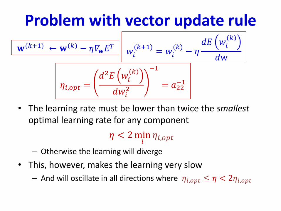
Problem with vector update rule
• The learning rate must be lower than twice the smallest optimal learning rate for any component
𝜂 < 2min𝑖𝜂𝑖,𝑜𝑝𝑡
– Otherwise the learning will diverge
• This, however, makes the learning very slow
– And will oscillate in all directions where 𝜂𝑖,𝑜𝑝𝑡 ≤ 𝜂 < 2𝜂𝑖,𝑜𝑝𝑡
𝐰(𝑘+1) ← 𝐰(𝑘) − 𝜂𝛻𝐰𝐸𝑇
𝑤𝑖(𝑘+1)
= 𝑤𝑖(𝑘)
− 𝜂𝑑𝐸 𝑤𝑖
(𝑘)
𝑑w
𝜂𝑖,𝑜𝑝𝑡 =𝑑2𝐸 𝑤𝑖
(𝑘)
𝑑𝑤𝑖2
−1
= 𝑎22−1
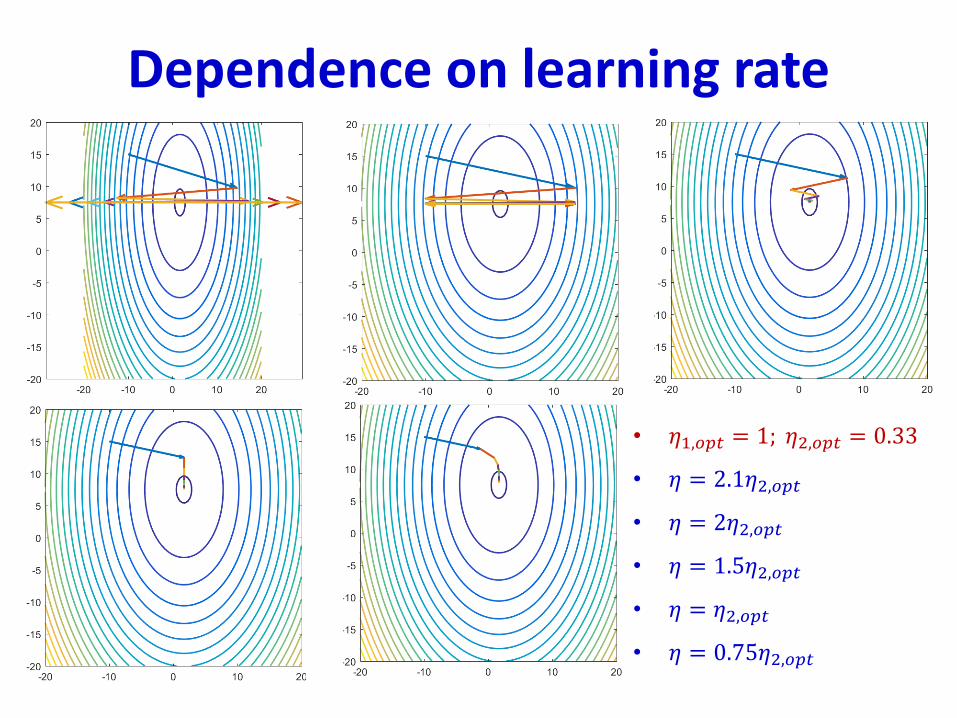
Dependence on learning rate
• 𝜂1,𝑜𝑝𝑡 = 1; 𝜂2,𝑜𝑝𝑡 = 0.33
• 𝜂 = 2.1𝜂2,𝑜𝑝𝑡
• 𝜂 = 2𝜂2,𝑜𝑝𝑡
• 𝜂 = 1.5𝜂2,𝑜𝑝𝑡
• 𝜂 = 𝜂2,𝑜𝑝𝑡
• 𝜂 = 0.75𝜂2,𝑜𝑝𝑡
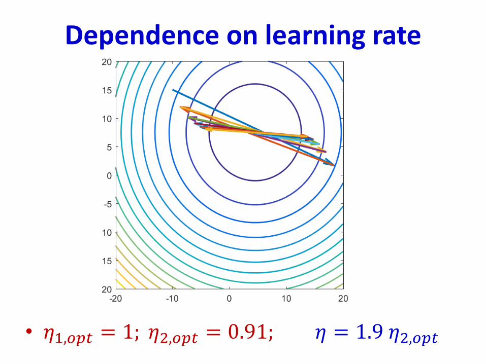
Dependence on learning rate
• 𝜂1,𝑜𝑝𝑡 = 1; 𝜂2,𝑜𝑝𝑡 = 0.91; 𝜂 = 1.9 𝜂2,𝑜𝑝𝑡
Convergence
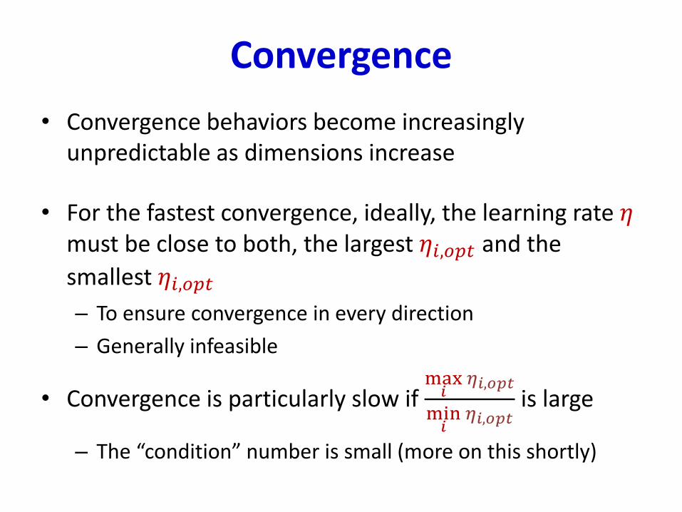
• Convergence behaviors become increasingly unpredictable as dimensions increase
• For the fastest convergence, ideally, the learning rate 𝜂must be close to both, the largest 𝜂𝑖,𝑜𝑝𝑡 and the
smallest 𝜂𝑖,𝑜𝑝𝑡– To ensure convergence in every direction
– Generally infeasible
• Convergence is particularly slow if max𝑖
𝜂𝑖,𝑜𝑝𝑡
min𝑖
𝜂𝑖,𝑜𝑝𝑡is large
– The “condition” number is small (more on this shortly)
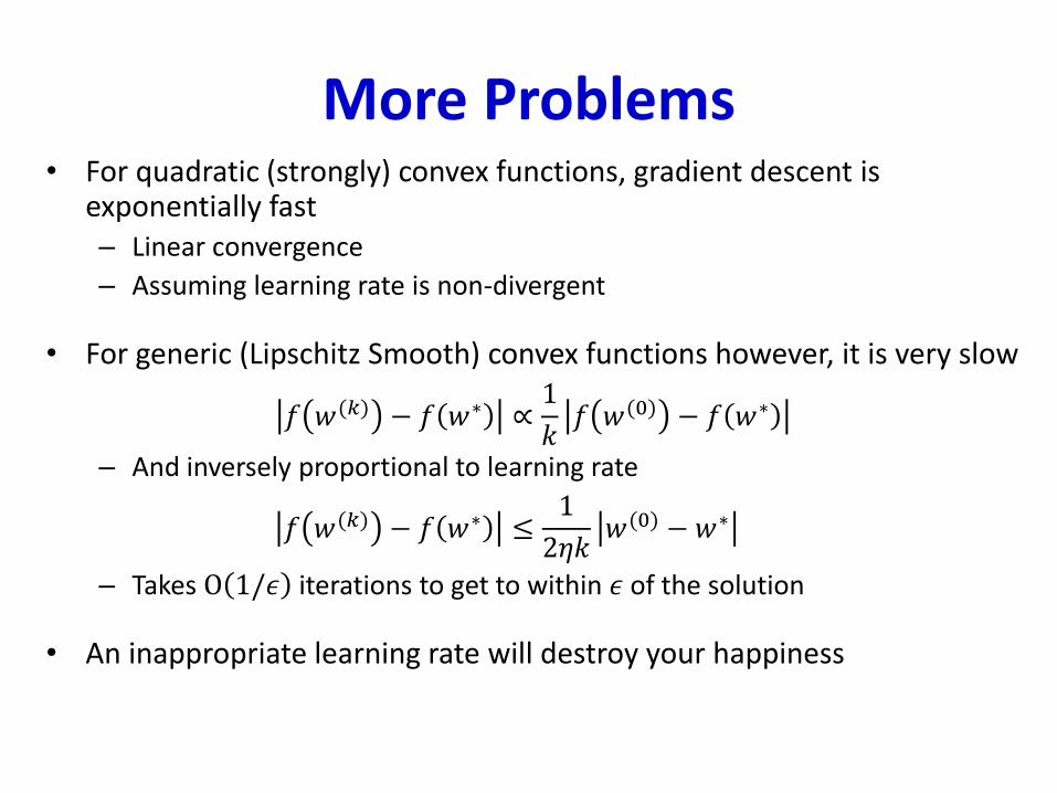
More Problems• For quadratic (strongly) convex functions, gradient descent is
exponentially fast– Linear convergence
– Assuming learning rate is non-divergent
• For generic (Lipschitz Smooth) convex functions however, it is very slow
𝑓 𝑤(𝑘) − 𝑓 𝑤∗ ∝1
𝑘𝑓 𝑤(0) − 𝑓 𝑤∗
– And inversely proportional to learning rate
𝑓 𝑤(𝑘) − 𝑓 𝑤∗ ≤1
2𝜂𝑘𝑤(0) − 𝑤∗
– Takes O 1/𝜖 iterations to get to within 𝜖 of the solution
• An inappropriate learning rate will destroy your happiness
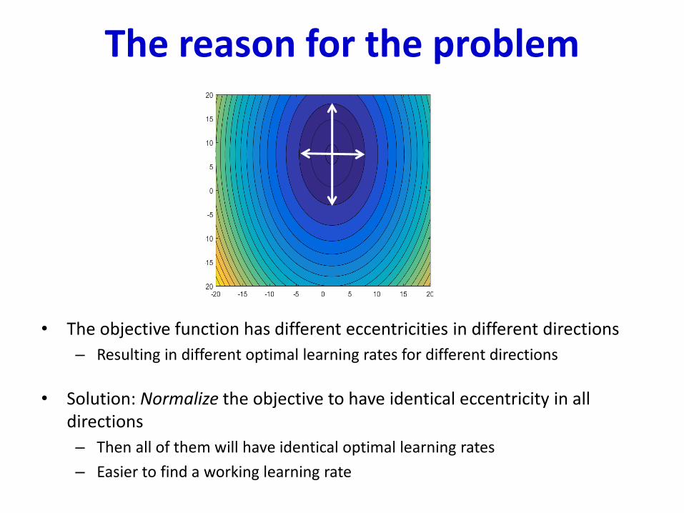
The reason for the problem
• The objective function has different eccentricities in different directions
– Resulting in different optimal learning rates for different directions
• Solution: Normalize the objective to have identical eccentricity in all directions
– Then all of them will have identical optimal learning rates
– Easier to find a working learning rate
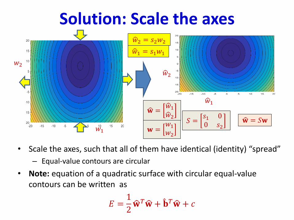
Solution: Scale the axes
• Scale the axes, such that all of them have identical (identity) “spread”
– Equal-value contours are circular
• Note: equation of a quadratic surface with circular equal-value contours can be written as
𝐸 =1
2ෝ𝐰𝑇 ෝ𝐰 + መ𝐛𝑇 ෝ𝐰 + 𝑐
𝑤1
𝑤2
ෝ𝑤1
ෝ𝑤2
ෝ𝑤1 = 𝑠1𝑤1
ෝ𝑤2 = 𝑠2𝑤2
ෝ𝐰 =ෝ𝑤1ෝ𝑤2
ෝ𝐰 = 𝑆𝐰
𝐰 =𝑤1𝑤2
𝑆 =𝑠1 00 𝑠2
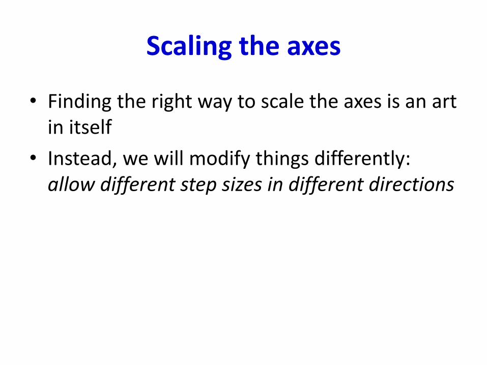
Scaling the axes
• Finding the right way to scale the axes is an art in itself
• Instead, we will modify things differently: allow different step sizes in different directions
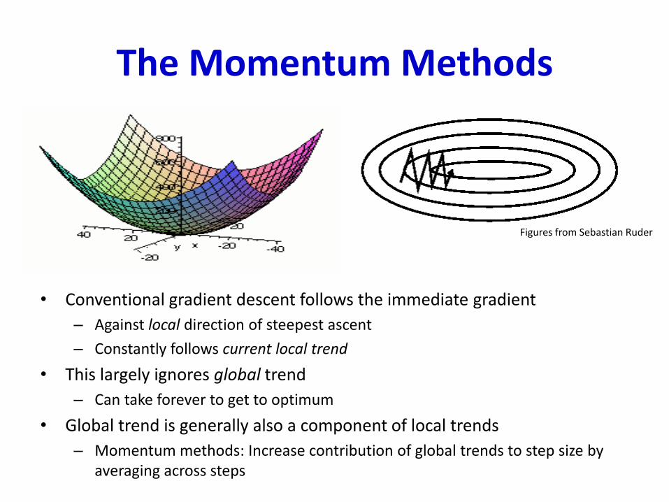
The Momentum Methods
• Conventional gradient descent follows the immediate gradient
– Against local direction of steepest ascent
– Constantly follows current local trend
• This largely ignores global trend
– Can take forever to get to optimum
• Global trend is generally also a component of local trends
– Momentum methods: Increase contribution of global trends to step size by averaging across steps
Figures from Sebastian Ruder
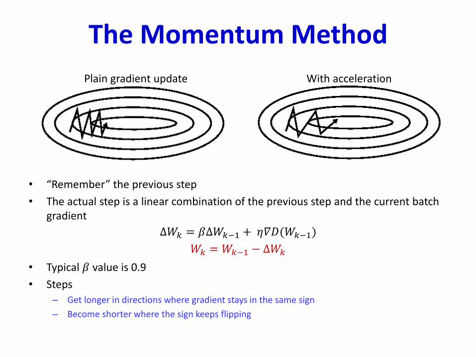
The Momentum Method
• “Remember” the previous step
• The actual step is a linear combination of the previous step and the current batch gradient
∆𝑊𝑘 = 𝛽∆𝑊𝑘−1 + 𝜂𝛻𝐷(𝑊𝑘−1)
𝑊𝑘 = 𝑊𝑘−1 − ∆𝑊𝑘
• Typical 𝛽 value is 0.9
• Steps – Get longer in directions where gradient stays in the same sign
– Become shorter where the sign keeps flipping
Plain gradient update With acceleration
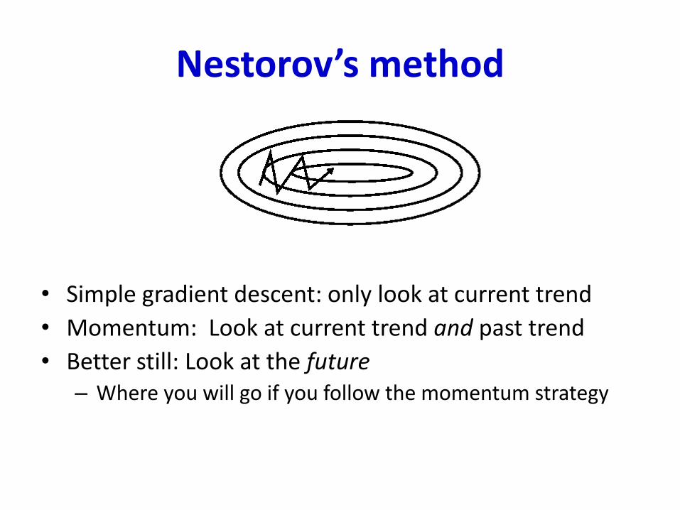
Nestorov’s method
• Simple gradient descent: only look at current trend
• Momentum: Look at current trend and past trend
• Better still: Look at the future– Where you will go if you follow the momentum strategy
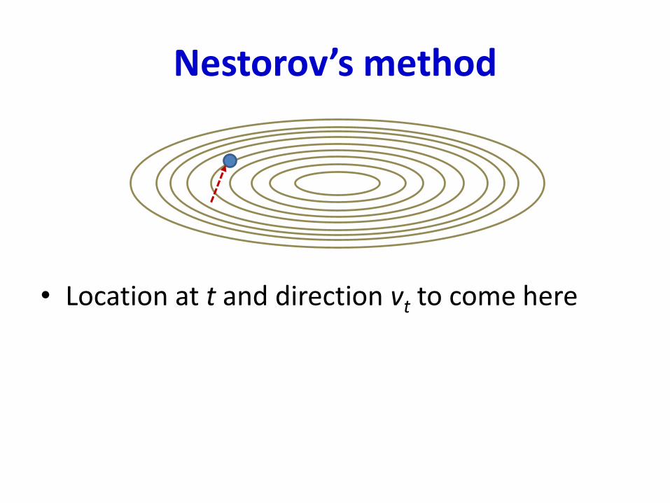
Nestorov’s method
• Location at t and direction vt to come here
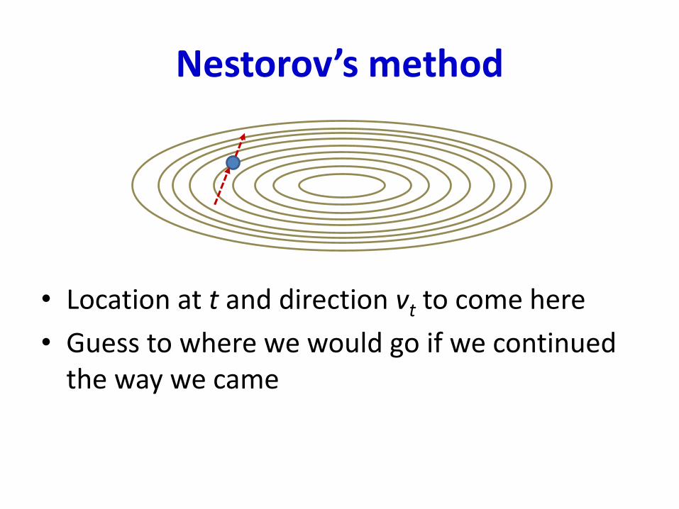
Nestorov’s method
• Location at t and direction vt to come here
• Guess to where we would go if we continued the way we came
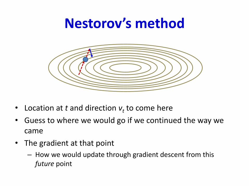
Nestorov’s method
• Location at t and direction vt to come here
• Guess to where we would go if we continued the way we came
• The gradient at that point
– How we would update through gradient descent from this future point
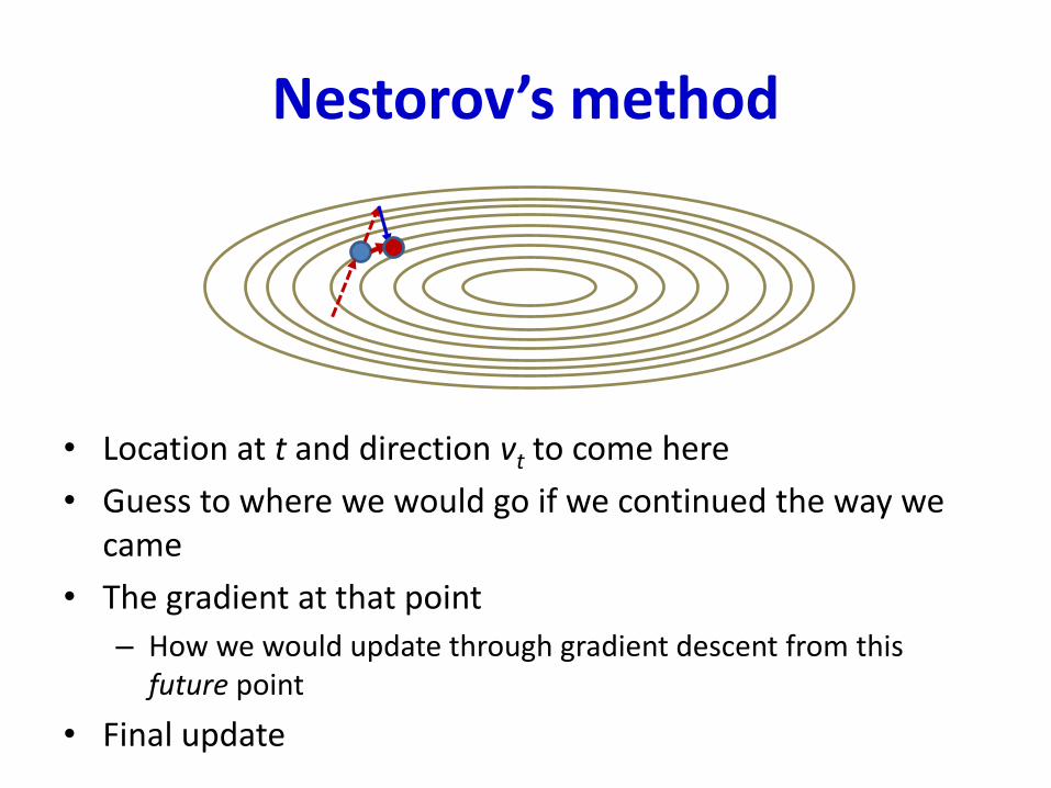
Nestorov’s method
• Location at t and direction vt to come here
• Guess to where we would go if we continued the way we came
• The gradient at that point
– How we would update through gradient descent from this future point
• Final update
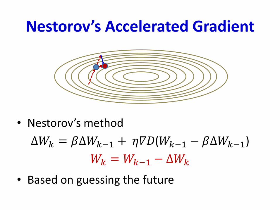
Nestorov’s Accelerated Gradient
• Nestorov’s method
∆𝑊𝑘 = 𝛽∆𝑊𝑘−1 + 𝜂𝛻𝐷(𝑊𝑘−1 − 𝛽∆𝑊𝑘−1)
𝑊𝑘 = 𝑊𝑘−1 − ∆𝑊𝑘
• Based on guessing the future
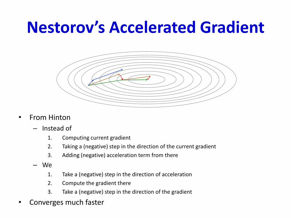
Nestorov’s Accelerated Gradient
• From Hinton
– Instead of 1. Computing current gradient
2. Taking a (negative) step in the direction of the current gradient
3. Adding (negative) acceleration term from there
– We1. Take a (negative) step in the direction of acceleration
2. Compute the gradient there
3. Take a (negative) step in the direction of the gradient
• Converges much faster
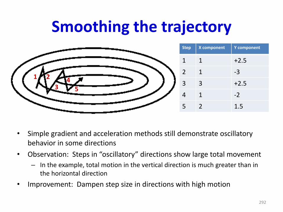
Smoothing the trajectory
• Simple gradient and acceleration methods still demonstrate oscillatory behavior in some directions
• Observation: Steps in “oscillatory” directions show large total movement
– In the example, total motion in the vertical direction is much greater than in the horizontal direction
• Improvement: Dampen step size in directions with high motion
292
1 2
34
5
Step X component Y component
1 1 +2.5
2 1 -3
3 3 +2.5
4 1 -2
5 2 1.5
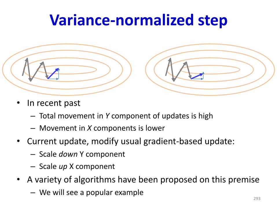
Variance-normalized step
• In recent past
– Total movement in Y component of updates is high
– Movement in X components is lower
• Current update, modify usual gradient-based update:
– Scale down Y component
– Scale up X component
• A variety of algorithms have been proposed on this premise
– We will see a popular example293
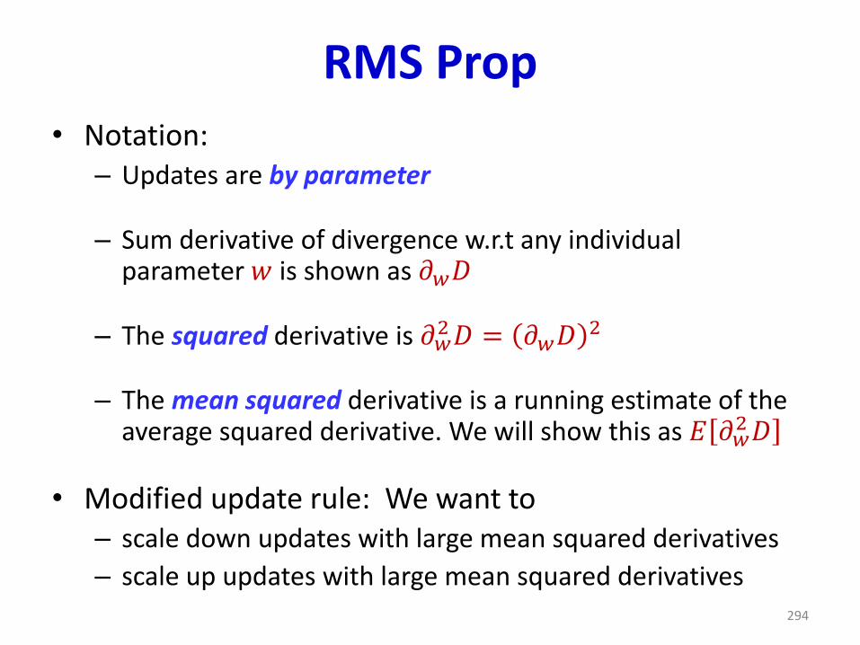
RMS Prop
• Notation:– Updates are by parameter
– Sum derivative of divergence w.r.t any individual parameter 𝑤 is shown as 𝜕𝑤𝐷
– The squared derivative is 𝜕𝑤2𝐷 = 𝜕𝑤𝐷
2
– The mean squared derivative is a running estimate of the average squared derivative. We will show this as 𝐸 𝜕𝑤
2𝐷
• Modified update rule: We want to – scale down updates with large mean squared derivatives
– scale up updates with large mean squared derivatives294
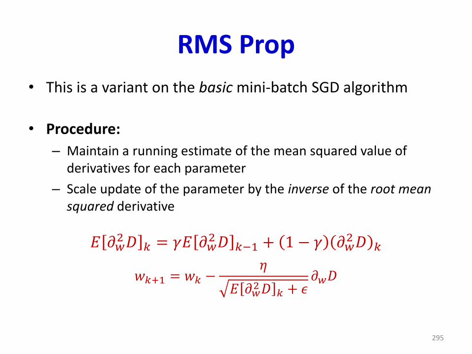
RMS Prop
• This is a variant on the basic mini-batch SGD algorithm
• Procedure:
– Maintain a running estimate of the mean squared value of derivatives for each parameter
– Scale update of the parameter by the inverse of the root mean squared derivative
𝐸 𝜕𝑤2𝐷 𝑘 = 𝛾𝐸 𝜕𝑤
2𝐷 𝑘−1 + 1 − 𝛾 𝜕𝑤2𝐷 𝑘
𝑤𝑘+1 = 𝑤𝑘 −𝜂
𝐸 𝜕𝑤2𝐷 𝑘 + 𝜖
𝜕𝑤𝐷
295
Fast convergence remains a challenge
• Newer methods:
– Adagrad
– AdaDelta
– RMS Prop
– ADAM
296
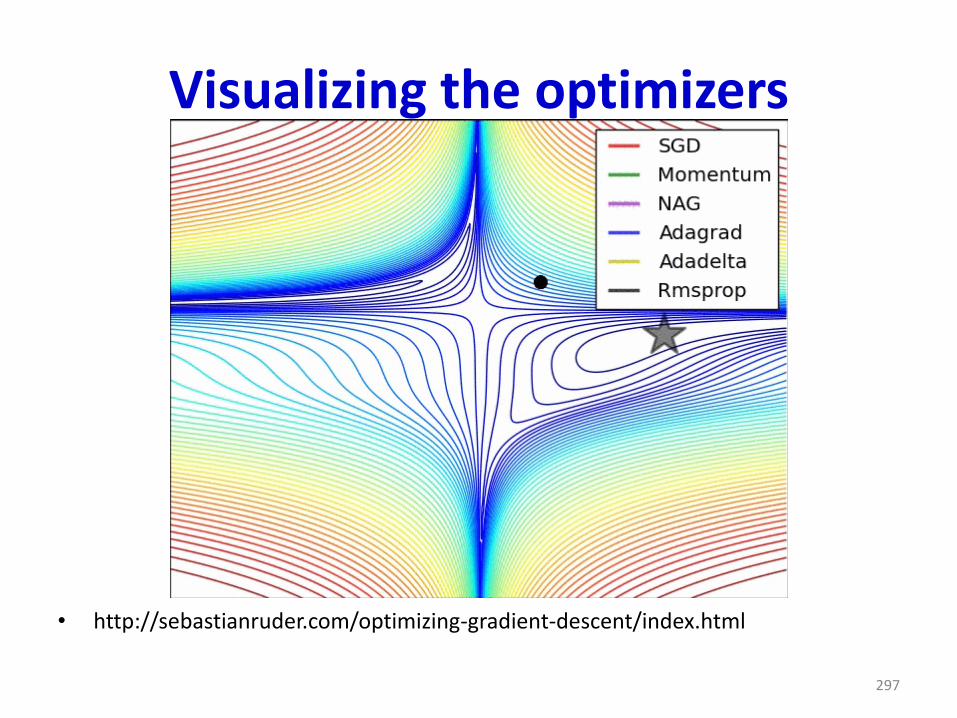
Visualizing the optimizers
• http://sebastianruder.com/optimizing-gradient-descent/index.html
297
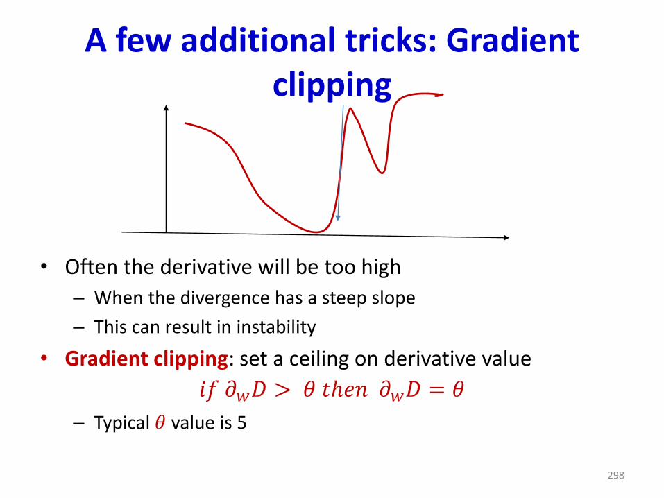
A few additional tricks: Gradient clipping
• Often the derivative will be too high
– When the divergence has a steep slope
– This can result in instability
• Gradient clipping: set a ceiling on derivative value
𝑖𝑓 𝜕𝑤𝐷 > 𝜃 𝑡ℎ𝑒𝑛 𝜕𝑤𝐷 = 𝜃
– Typical 𝜃 value is 5
298
Several other tricks are often required for good performance
• Batch normalization
• Dropout
• Other issues not covered:
• Objective functions, speed up algorithms, generalization..
299
Far from complete
• Efficient training remains a challenge with much scope for advances..
300


![Deep Parametric Continuous Convolutional Neural Networks€¦ · Graph Neural Networks: Graph neural networks (GNNs) [25] are generalizations of neural networks to graph structured](https://img.pdfslide.us/doc/110x75/5f7096c356401635d36dbe30/deep-parametric-continuous-convolutional-neural-networks-graph-neural-networks.jpg)