Intro to DB CHAPTER 13 QUERY OPTIMIZATION

CHAPTER 13

QUERY OPTIMIZATION

Intro to DB

Original Slides:

© Silberschatz, Korth and Sudarshan

Intro to DB

Copyright © by S.-g. Lee Chap 13 - 2

Chapter 13: Query Optimization

▪ Overview

▪ Transformation of Relational Expressions

▪ Estimating Statistics of Expression Results

▪ Choice of Evaluation Plans

▪ Materialized Views

▪ Advanced Topics

Original Slides:


Intro to DB


Basic Steps in Query Processing

1. Parsing and translation

2. Optimization

3. Evaluation

Original Slides:


Intro to DB


Query Evaluation Plan

▪ An evaluation plan defines exactly what algorithm is used for each

operation, and how the execution of the operations is coordinated.

Original Slides:


Intro to DB


▪ Equivalence of Expressions

Given a DB schema S, a query Q on S is equivalent to another query

Q’ on S, if the answer sets of Q and Q’ are the same in any instances

of the DB.

name, title(dept=“Music”( instructor ⋈ (teaches ⋈ course ))) vs

name, title( (dept=“Music”(instructor)) ⋈ teaches ⋈ course )

Query Optimization

Original Slides:


Intro to DB


▪ Generation of query-evaluation plans for an expression involves

several steps:

1. Generating logically equivalent expressions

Use equivalence rules to transform an expression into an equivalent one.

2. Annotating resulting expressions to get alternative query plans

3. Choosing the cheapest plan based on estimated cost

▪ The overall process is called cost based optimization.

▪ Query optimization is the process of selecting the most efficient

query evaluation plan for a given query

A plan with the smallest estimated cost of execution

In a centralized system, disk access is the predominant cost

Generation of Evaluation Plan

Original Slides:


Intro to DB


Equivalence Rules

1. Conjunctive selection operations can be deconstructed into a

sequence of individual selections.

1 2 (E) = 1(2(E))

2. Selection operations are commutative.

1(2(E)) = 2(1(E))

3. Only the last in a sequence of projection operations is needed, the

others can be omitted.

t1(t2( … tn(E ) … )) = t1(E )

4. Selections can be combined with Cartesian products and theta joins.

a. (E1 X E2) = E1 ⋈ E2

b. 1(E1 ⋈2 E2) = E1 ⋈1 2 E2

Original Slides:


Intro to DB


Equivalence Rules (cont.)

5. Theta-join operations (and natural joins) are commutative.

E1 ⋈ E2 = E2 ⋈ E1

6. (a) Natural join operations are associative:

(E1 ⋈ E2) ⋈ E3 = E1 ⋈ (E2 ⋈ E3)

(b) Theta joins are associative in the following manner:

(E1 ⋈1 E2) ⋈2 3 E3 = E1 ⋈1 3 (E2 ⋈2 E3)

where 2 involves attributes from only E2 and E3.

Original Slides:


Intro to DB


Equivalence Rules (cont.)

7. Selection operation distributes over theta join

(a) when all the attributes in 0 involve only the attributes of one of

the expressions (E1) being joined.

0(E1 ⋈ E2) = (0(E1)) ⋈ E2

(b) when 1 involves only the attributes of E1 and 2 involves only the

attributes of E2.

12 (E1 ⋈ E2) = (1(E1)) ⋈ (2(E2))

Original Slides:


Intro to DB


Transformation – Example 1

▪ Query:

Find the names of all instructors in the Music department, along with

the titles of the courses that they teach.

name, title(dept=“Music” (instructor ⋈ (teaches ⋈ course)))

▪ Transformation using rule 7a.

name, title( (dept=“Music”(instructor) ⋈ (teaches ⋈ course) )

▪ Performing the selection as early as possible reduces the size of the

relation to be joined.

Original Slides:


Intro to DB


▪ Query: Find the names of all instructors in the Music department

who have taught a course in 2009, along with the titles of the

courses that they taught.

name, title(dept=“Music”year = 2009

(instructor ⋈ (teaches ⋈ c_id, title (course))))

▪ Using join associativity (Rule 6a):

name, title(dept=“Music”year = 2009

((instructor ⋈ teaches) ⋈ c_id, title (course))))

▪ Push selection in (Rules 7a & 7b):

name, title( (dept=“Music”(instructor) ⋈ year = 2009(teaches)) ⋈

c_id, title (course))))

Transformation – Example 2

Original Slides:


Intro to DB


Transformation – Example 2 (cont.)

Original Slides:


Intro to DB


▪ (r1 ⋈ r2) ⋈ r3 = r1 ⋈ (r2 ⋈ r3 ) (Rule 6a)

▪ Choose the expression that will yield smaller temporary result

▪ Example

name, title( ( dept=“Music”(instructor) ⋈ teaches ) ⋈

c_id, title (course) )

dept=“Music”(instructor) ⋈ teaches

vs

teaches ⋈ c_id, title (course)

Join Ordering

Original Slides:


Intro to DB


Cost Estimation

▪ Cost of computing each operator is as described in Chapter 12

Need statistics of input relations

E.g. number of tuples, sizes of tuples

▪ Inputs can be results of sub-expressions

Need to estimate size of expression results

To do so, we require additional statistics

E.g. number of distinct values for an attribute

▪ Recall that

Typically disk access is the predominant cost.

▪ We do not include cost of writing the final output to disk

▪ We refer to the cost estimate of algorithm A as EA

Original Slides:


Intro to DB


▪ nr: number of tuples in a relation r

▪ br: number of blocks containing tuples of r

br = nr/fr , if tuples of r are stored together physically in a file

▪ lr: size of a tuple of r

▪ fr: blocking factor of r

i.e., the number of tuples of r that fit into one block

▪ V(A, r): number of distinct values that appear in r for attribute A;

same as the size of A(r)

▪ SC(A, r): selection cardinality of attribute A of relation r; average

number of records that satisfy equality on A

Statistics for Cost Estimation

Original Slides:


Intro to DB


Catalog Information about Indices

▪ fi: average fan-out of internal nodes of index i,

for tree-structured indices such as B+-trees

▪ HTi: number of levels in index i — i.e., the height of i

For a balanced tree index (such as B+-tree) on attribute A of relation r,

HTi = logfi (V(A,r)).

For a hash index, HTi is 1.

LBi: number of lowest-level index blocks in i — i.e, the number of blocks

at the leaf level of the index.

Original Slides:


Intro to DB


Histograms

▪ Histogram on attribute age of relation person

▪ Equi-width histograms

▪ Equi-depth histograms

Original Slides:


Intro to DB


▪ Equality selection A=v(r)

SC(A, r) : number of records that will satisfy the selection

= nr / V(A,r) general case

= 1 (if A is key)

SC(A, r)/fr— number of blocks that these records will occupy

E.g. Binary search cost estimate becomes

EA = log2(br) * (tT + tS) + ( SC(A, r) / fr - 1 ) * tT

Selection Size Estimation

Original Slides:


Intro to DB


Join Operation: Running Example

Running example:

student ⋈ takes

Catalog information for join examples:

▪ nstudent = 5,000.

▪ fstudent = 50, which implies that bstudent =5000/50 = 100.

▪ ntakes = 10000.

▪ ftakes = 25, which implies that btakes = 10000/25 = 400.

▪ V(ID, takes) = 2500, which implies that on average, each student who has

taken a course has taken 4 courses.

Attribute ID in takes is a foreign key referencing student.

▪ V(ID, student) = 5000 (primary key!)

Original Slides:


Intro to DB


▪ r ⋈ s = r x s if R S =

r x s contains nr * ns tuples

each tuple occupies lr + ls bytes

▪ If R S is a key for R

then a tuple of s will join with at most one tuple from r

therefore, the number of tuples in r ⋈ s is no greater than the number

of tuples in s.

In the example query student ⋈ takes

ID in takes is a foreign key of student

hence, the result has (exactly) ntakes = 10,000 tuples

Join Size Estimation

Original Slides:


Intro to DB


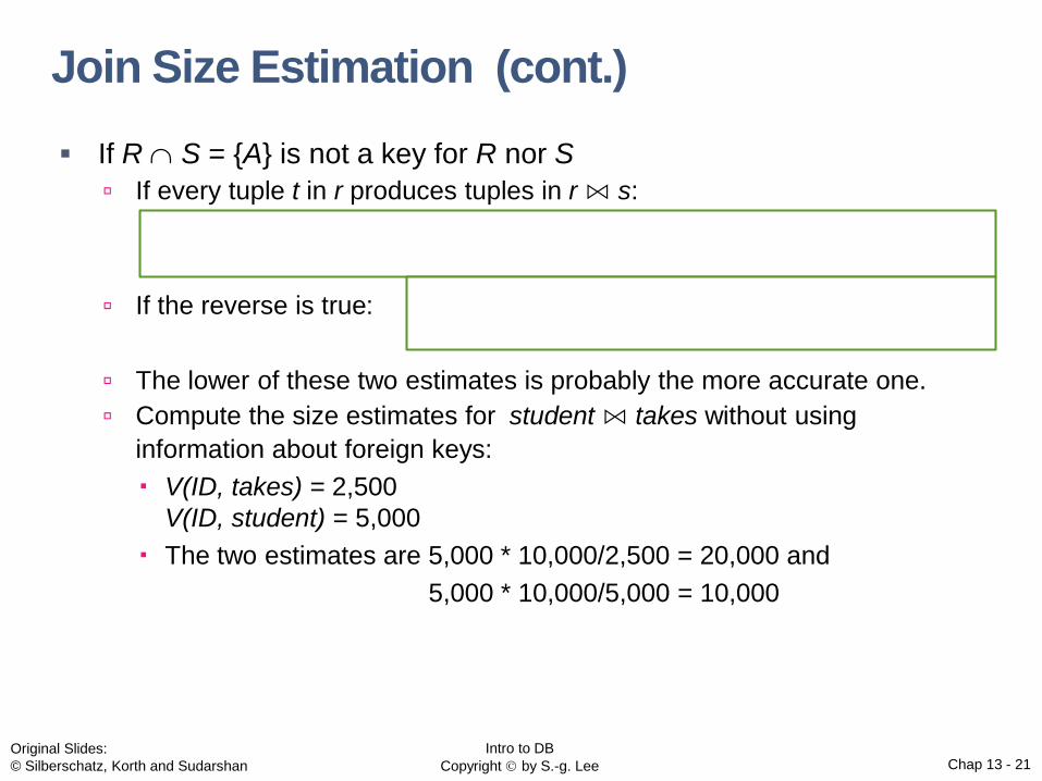
▪ If R S = {A} is not a key for R nor S

If every tuple t in r produces tuples in r ⋈ s:

( nr * ns ) / V(A, s)

If the reverse is true: ( nr * ns ) / V(A, r)

The lower of these two estimates is probably the more accurate one.

Compute the size estimates for student ⋈ takes without using

information about foreign keys:

V(ID, takes) = 2,500

V(ID, student) = 5,000

The two estimates are 5,000 * 10,000/2,500 = 20,000 and

5,000 * 10,000/5,000 = 10,000

Join Size Estimation (cont.)

Original Slides:


Intro to DB


Cost Estimation of Expressions

bcourse = 10000/25 = 400

binstructor = 2000/25 = 80

bteaches = 20000/100 = 200(20%)

M = 22

N: br / (M-2) bs + br

H: 3(br + bs) + 4nh

(1%)

Original Slides:


Intro to DB


Cost Estimation of Expressions

bcourse = 10000/25

= 400 blocks

binstructor = 1000/25

= 80 blocksbteaches = 20000/100

= 200 blocks

(20%)

(1%)

Original Slides:


Intro to DB


Choice of Evaluation Plans

▪ Must consider the interaction of evaluation techniques when

choosing evaluation plans

choosing the cheapest algorithm for each operation independently may

not yield best overall algorithm.

merge-join may be costlier than hash-join, but may provide a sorted output

which reduces the cost for an outer level aggregation.

nested-loop join may provide opportunity for pipelining

▪ Practical query optimizers incorporate elements of the following two

broad approaches:

1. Search all the plans and choose the best plan in a

cost-based fashion.

2. Uses heuristics to choose a plan.

Original Slides:


Intro to DB


Cost-Based Optimization

▪ Consider finding the best join-order for r1 ⋈ r2 ⋈ … ⋈ rn.

▪ There are

(2(n – 1))!/(n – 1)! different join orders

for above expression.

with n = 7, the number is 665280

with n = 10, the number is > 176 billion!

▪ Can reduce search space using dynamic programming

Using dynamic programming, the least-cost join order for any subset of

{r1, r2, . . . rn} is computed only once and stored for future use.

Time complexity of optimization with bushy trees is O(3n)

Space complexity: O(2n)

With n = 10, this number is 59,000 (instead of 176 billion!)

Original Slides:


Intro to DB


Heuristic Optimization

▪ Cost-based optimization is expensive, even with dynamic

programming

Search space grows exponentially!

▪ Heuristic optimization

make transformations based on a set of rules that typically (but not in all

cases) improve execution performance:

Perform selection early (reduces the number of tuples)

Perform projection early (reduces the number of attributes)

Perform most restrictive selection and join operations before other similar

operations

Some systems use only heuristics, others combine heuristics with partial

cost-based optimization.

Original Slides:


Intro to DB


Left Deep Join Trees

▪ In left-deep join trees, the right-hand-side input for each join is a

relation, not the result of an intermediate join.

▪ If only left-deep trees are considered, time complexity of finding best join order is O(n 2n)

n=10 => 10,000 (cf. 59,000 or 176 billion)

Space complexity remains at O(2n)

END OF CHAPTER 13

Documents

Intro to DB CHAPTER 13 QUERY OPTIMIZATION