Embed Size (px)
Citation preview

Intro to AI , Fall 2004 [email protected] 1
Introduction to Artificial Intelligence
LECTURE 4: Informed Search
• What is informed search?
• Best-first search
• A* algorithm and its properties
• Iterative deepening A* (IDA), SMA*
• Hill climbing and simulated annealing
• AO* algorithm for AND/OR graphs

Intro to AI , Fall 2004 [email protected] 2
Drawbacks of uninformed search• Criterion to choose next node to expand
depends only on the level number.
• Does not exploit the structure of the problem.
• Expands the tree in a predefined way. It is not adaptive to what is being discovered on the way, and what can be a good move.
• Very often, we can select which rule to apply by comparing the current state and the desired state.

Intro to AI , Fall 2004 [email protected] 3
Uninformed search
A
3
2
1
Suppose we know that node A is very promising
Why not expand it right away?
StartGoal

Intro to AI , Fall 2004 [email protected] 4
Informed search: the idea
• Heuristics: search strategies or rules of thumb that bring us closer to a solution MOST of the time
• Heuristics come from the structure of the problem, and are aimed to guide the search
• Take into account the cost so far and the estimated cost to reach the goal
heuristic cost function

Intro to AI , Fall 2004 [email protected] 5
Informed search -- version 1
A
2
1
A is estimated to be very close to the goal
expand it right away!!
StartGoal
Estimate_Cost(Node, Goal)

Intro to AI , Fall 2004 [email protected] 6
Informed search -- version 2
A
2
1
A has cost the least to reach. Expand it first!
StartGoal
Cost_so_far(Node, Goal)

Intro to AI , Fall 2004 [email protected] 7
Informed search: issues
• What are the properties of the heuristic function?– is it always better than choosing randomly?– when it does not, how bad can it get?– does it guarantee that if a solution exist, we will
find it?– is the path optimal?
• Choosing the right heuristic function makes all the difference!

Intro to AI , Fall 2004 [email protected] 8
Best first searchfunction Best-First-Search(problem,Eval-FN)
returns solution sequence
nodes := Make-Queue(Make-Node(Initial-State(problem))
loop do if nodes is empty then return failure
node := Remove-Front(nodes)
if Goal-Test[problem] applied to State(node) succeeds
then return node
new-nodes := Expand(node, Operarors[problem],
Eval-FN)))
nodes := Insert-by-Cost(new-nodes,Eval-FN(new-node))
end
Intro to AI , Fall 2004 [email protected] 9
Illustration of Best First Search
2
1
Start
Goal
Not expanded yet
Leaf nodes in queue
Expanded before
4
3

Intro to AI , Fall 2004 [email protected] 10
A graph search problem...
S
A B C
D E F
G
3
4
5
2
5
4 4
4
3
G

Intro to AI , Fall 2004 [email protected] 11
Straight-line distances to goalS
A D
B D A E
C E E B B F
D F B F C E A C G
G C G F
G
10.4 8.4
6.7 8.9 10.4 6.9
6.9 6.9 6.7 6.7 3.0
3.0 6.7 3.0 4.0 6.9 10.4 4.0 0.0
0.0 4.0 0.0 3.0
0.0

Intro to AI , Fall 2004 [email protected] 12
Example of best first search strategy
A
A
D
E
S
B F
G
10.4 8.4
10.4 6.9
3.06.7Heuristic function:
Straight line distance from goal
Intro to AI , Fall 2004 [email protected] 13
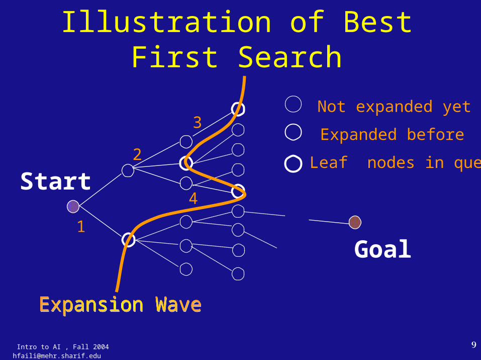
Greedy search• Expand the node with the lowest expected cost
• Choose the most promising step locally
• Not always guaranteed to find an optimal solution -- it depends on the function!
• Behaves like DFS: follows to depth paths that look promising
• Advantage: moves quickly towards the goal
• Disadvantage: can get stuck in deep paths
• Example: the previous graph search strategy!

Intro to AI , Fall 2004 [email protected] 14
Branch and bound• Expand the node with the lowest cost so far
• No heuristic is used, just the actual elapsed cost so far
• Behaves like BFS if all costs are uniform
• Advantage: minimum work. Guaranteed to finds the optimal solution because the path is shortest!
• Disadvantage: does not take into account the goal at all!!

Intro to AI , Fall 2004 [email protected] 15
Branch and bound on the graphS
A D
B D A E
C E E B B F
D F B F C E A C G
G C G F
G
3 4
7 9 6
13 10 13 11 10
17 15 14 17 18 15 15 13
20 19 17 22
25
8
1 2
534
6
Heuristic function:
distance so far

Intro to AI , Fall 2004 [email protected] 16
A* Algorithm -- the idea
• Combine the advantages of greedy search and branch and bound:
(cost so far) AND (expected cost to goal)
• Intuition: it is the SUM of both costs that ultimately matters
• When the expected cost is an exact measure, the strategy is optimal
• The strategy has provable properties for certain classes of heuristic functions

Intro to AI , Fall 2004 [email protected] 17
A* Algorithm -- formalization (1)
• Two functions– cost from start: g(n) always accurate– expected cost to goal: h(n) an estimate
• Heuristic function f(n) = g(n) + h(n)
• Strategy min f(n)
• f * is the cost of the optimal path
• h*(n) and f*(n) are the optimal path costs through node n (not necessarily the absolute optimal cost)

Intro to AI , Fall 2004 [email protected] 18
A* Algorithm -- formalization (2)
• The expected cost h(n) can always underestimate, always overestimates, or both
• Admissible condition: the estimated cost to goal always underestimates of the real cost (it is always optimistic)
h(n) <= h*(n)
• when h(n) is admissible, so is f(n):f(n) <= f*(n) and g(n) = g*(n)

Intro to AI , Fall 2004 [email protected] 19
Example: graph search
Heuristic function:
Distance so far + straight line distance from goal
A
A
D
E
S
B F
G
13.4 12.4
19.412.9
13.017.7
(=3+10.4)(=4+8.4)
(=6+6.9)(=9+10.4)
(=11+6.7)
13.0(=13+0.0)
(=10+3)
11.9 (=0+11.9)

Intro to AI , Fall 2004 [email protected] 20
A* algorithm
• Best-First-Search with Eval-FN(node) = g(node) + h(node)
• Termination condition: after a goal is found (at cost c), expand open nodes until each of their g+h values is greater than or equal to c to guarantee optimality
• Extreme cases:– h(n) = 0 Branch-and-Bound– g(n) = 0 Greedy search– h(n) = 0 and g(n) = 0 Uninformed search

Intro to AI , Fall 2004 [email protected] 21
Proof of A* optimality (1)• Lemma: at any time before A* terminates,
there exists a node n’ in the OPEN nodes queue such that f(n’) <= f*
• Proof: Let P*(n’) be an optimal path through n’ from the start node to the goal nodeP*(n’) = s, n1,n2,…n’,…goal and let n’ be the best node in OPEN The path s….n’ where g(n’) = g*(n’) is the optimal so far by construction

Intro to AI , Fall 2004 [email protected] 22
Proof of A* optimality (2)
For any node n’ in the optimal path from start to
goal
Therefore, f(n’) <= f*
Theorem: A* produces the optimal path.
Proof by contradiction
Suppose A* terminates with goal node t such that f(t) > f*

Intro to AI , Fall 2004 [email protected] 23
Proof of A* optimality (3)When t was chosen for expansion,
f(t) <= f(n) for all n in OPEN
Thus, f(n) > f* at this stage.
This contradicts the lemma, which states that there is always at least one node n’ in OPEN such that f(n’) <= f*
Other properties:– A* expands all nodes such that – A* expands the minimum number of nodes

Intro to AI , Fall 2004 [email protected] 24
A* monotonicity• When f(n) never decreases as the search
progresses, it is said to be monotone• If f(n) is monotone, then A* has already found
an optimal path for the node it expands (prove)
• Monotonicity simplifies termination condition: the first solution it finds is optimal
• If f(n) is not monotone, fix it with:f(n) = max(f(m), g(n) + h(n))
where m is a parent of n. Use the cost of the parent when the estimate is not decreasing

Intro to AI , Fall 2004 [email protected] 25
A* is complete
• Since A* expands nodes in increasing order of f value, it must eventually expand to reach the goal state if there are finitely many nodes such that f(n) < f*
– finite branching factor– path with a finite cost but infinitely many nodes
• A* is complete on locally finite graphs (finite branching factor, each operation costs, the sum of costs is not asymptotically bounded)

Intro to AI , Fall 2004 [email protected] 26
Complexity of A*
• A* is exponential in time and memory: the OPEN nodes queue grows exponentially on average O(bd).
• Condition for subexponential growth:| h(n) - h*(n) | <= O(log h*(n))
where h* is the true cost from n to the goal
• For must heuristics, the error is at least proportional to the path cost….

Intro to AI , Fall 2004 [email protected] 27
Comparing heuristic functions
• Bad estimates of the remaining distance can cause extra work!
• Given two algorithms A1 and A2 with admissible heuristics h1 and h2 < h*(n) which one is best?
• Theorem: if h1(n) < h2(n) for all non-goal nodes n, then A1 expands at least as many nodes as A2
We say that A2 is more informed than A1

Intro to AI , Fall 2004 [email protected] 28
Example: 8-puzzle• h1: number of tiles in the wrong position
• h2: sum of the Manhattan distances from their goal positions (no diagonals)
• which one is best? h1 = 7
h2 = 19
(2+3+3+3+4+2+0+2)

Intro to AI , Fall 2004 [email protected] 29
Performance comparison
Note: there are better heuristics for the 8-puzzle...

Intro to AI , Fall 2004 [email protected] 30
How to come up with heuristics?• Consider relaxed versions of the problem:
remove constraints, – 8-puzzle: tiles cannot overlap– Graph search: straight line distance
• Assign weights: f(n) = w1.g(n) + w2.h(n), w1+w2=1
• Combine several functions: f(n) = F(f1(n),f2(n),…,fk(n)), F = max, sum
• Apply cheapest heuristic function

Intro to AI , Fall 2004 [email protected] 31
IDA*: Iterative deepening A*
• To reduce the memory requirements at the expense of some additional computation time, combine uninformed iterative deepening search with A*
(IDS expands in DFS fashion trees of depth 1,2, …)
• Use an f-cost limit instead of a depth limit

Intro to AI , Fall 2004 [email protected] 32
IDA* Algorithm - Top level
function IDA*(problem) returns solution
root := Make-Node(Initial-State[problem])
f-limit := f-Cost(root)
loop do
solution, f-limit := DFS-Contour(root, f-limit)
if solution is not null, then return solution
if f-limit = infinity, then return failure
end

Intro to AI , Fall 2004 [email protected] 33
IDA* contour expansion
function DFS-Countour(node,f-limit) returns
solution sequence and new f-limit
if f-Cost[node] > f-limit then return (null, f-Cost[node] )
if Goal-Test[problem](State[node]) then return (node,f-limit)
for each node s in Successor(node) do
solution, new-f := DFS-Contour(s, f-limit)
if solution is not null, then return (solution, f-limit)
next-f := Min(next-f, new-f); end
return (null, next-f)

Intro to AI , Fall 2004 [email protected] 34
IDA* on graph example
B D A E
C E E B B F
D F B F C E A C G
G C G F
G
13.7 16.9 19.4 12.9
19.9 16.9 19.7 17.7 13.0
20.0 21.7 17.0 21.0 24.9 25.4 19.0 13.0
0.0 4.0 0.0 3.0
0.0
S
A D13.4 12.4
11.9
14.0
14.0

Intro to AI , Fall 2004 [email protected] 35
IDA* traceIDA(S, 11.9)Level 0:
Level 1: IDA(A, 11.9)IDA(S, 11.9)
IDA(D, 11.9) 12.4
IDA(A, 12.4)IDA(S, 12.4)
IDA(D, 12.4)
13.4
19.4 IDA(A, 12.4)
IDA(E, 12.4)
12.9
Level 2:
Level 3:
13.4
11.9
IDA(S, 12.9) IDA(F, 12.9) 13.0

Intro to AI , Fall 2004 [email protected] 36
Simplified Memory-Bounded A*• IDA* repeats computations, but only keeps bd
nodes in the queue.
• When more memory is available, more nodes can be kept, and avoid repeating those nodes
• Need to delete nodes from the A* queue (forgotten nodes). Drop those with higher f-cost values first
• Remember ancestor nodes information about best path so far, so those with lower values will be expanded next

Intro to AI , Fall 2004 [email protected] 37
SMA* mode of operation
• Expand deepest least cost node
• Forget shallowest highest cost
• Remember value of best forgotten successor
• Non-goal at maximum depth is infinity
• Regenerates a subtree only when all other paths have been shown to be worse than the path it has forgotten.

Intro to AI , Fall 2004 [email protected] 38
SMA* properties• Checks for repetitions of nodes in memory
• Complete when there is enough space to store the shallowest solution path
• Optimal if enough memory available for the shallowest optimal solution path. Otherwise, it returns the best solution reachable with available memory
• When enough memory for the entire search tree, search is optimally efficient (A*)

Intro to AI , Fall 2004 [email protected] 41
Iterative improvement algorithms• What if the goal is not known? We only know
how to compare two states and say which one is best:– earn as much money as possible– pack the tiles in the smallest amount of space– reduce the number of conflicts in a schedule
• Start with a legal state, and try to improve it
• Cannot guarantee to find the optimal solution, can produce the best solution so far
• Minimization/maximization problem

Intro to AI , Fall 2004 [email protected] 42
Hill climbing strategy
• Apply the rule that increases the most the current state value
• Move in the direction of the greatest gradient
states
f-value
while f-value(state) > f-value(best-next(state))
state := next-best(state)

Intro to AI , Fall 2004 [email protected] 43
Hill climbing -- Properties
• Called gradient descent method in optimization
• Will stop at a local maximum (minimum) with no clue on how to proceed next
• Performs random search for equal values (plateau)
• Requires a strategy for escaping a local minimum: random jump, backtrack, etc

Intro to AI , Fall 2004 [email protected] 44
Simulated annealing• Proceed like hill climbing, but pick at each
step a random move
• If the move improves the f-value, it is always executed
• Otherwise, it is executed with a probability that decreases exponentially as improvement is not found
• Probability function: – T is the number of steps since improvement
– is the amount of decrease at each step

Intro to AI , Fall 2004 [email protected] 45
Simulated annealing algorithmfunction Simulated-Annealing(problem, schedule) returns
solution state
current := Make-Node(Initial-State[problem])
for t := 1 to infinity
T := schedule[t]
if T = 0 then return current
next := Random-Successor(current)
:= f-Value[next] - f-Value[current]
if > 0 then current := next
else current := next with probability
end

Intro to AI , Fall 2004 [email protected] 46
Analogy to physical process• Annealing is the process of cooling a liquid
until it freezes (E energy, T temperature).
• The schedule is the rate at which the temperature is lowered
• Individual moves correspond to random fluctuations due to termal noise
• One can prove that if the temperature is lowered sufficiently slowly, the material will attain its state of lowest energy configuration (global minimum)

Intro to AI , Fall 2004 [email protected] 47
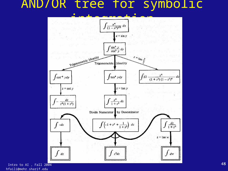
AND/OR graphs
• Some problems are best represented as achieving subgoals, some of which achieved simultaneously and independently (AND)
• Up to now, only dealt with OR options
Possess TV set
Steal TV Earn Money Buy TV

Intro to AI , Fall 2004 [email protected] 49
Grammar parsing
F EA
F DD
E DC
E CD
D F
D A
C A
A a
D d
F
E A D D
D C C D
A A
A A
Is the string ada in the language?

Intro to AI , Fall 2004 [email protected] 50
Searching AND/OR graphs• Hyperhgraphs: OR and AND connectors to
several nodes - consider trees only
• Generate nodes according to AND/OR rules
• A solution in an AND-OR tree is a subtree (before, a path) whose leafs (before, a single node) are included in the goal set
• Cost function: sum of costs in AND nodef(n) = f(n1) + f(n2) + …. + f(nk)
• How can we extend Best-First-Search and A* to search AND/OR trees? The AO* algorithm.
Intro to AI , Fall 2004 [email protected] 51
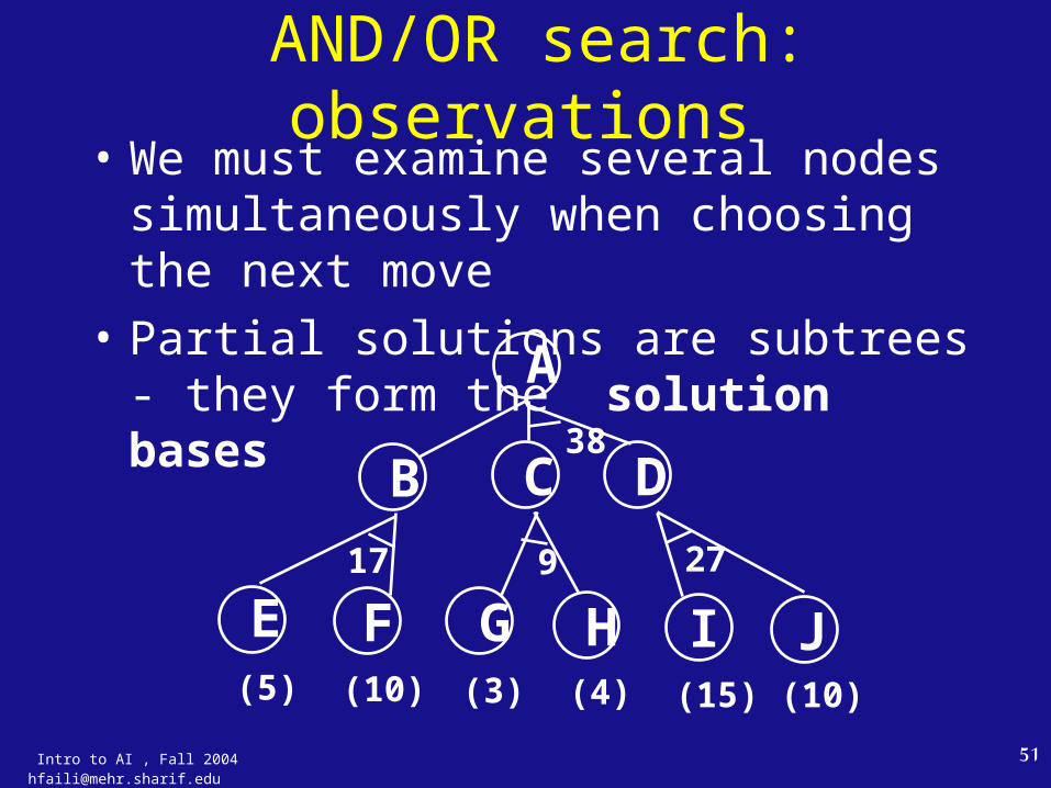
AND/OR search: observations • We must examine several nodes
simultaneously when choosing the next move
• Partial solutions are subtrees - they form the solution bases A
B C D38
E F G H I J
17 9 27
(5) (10) (3) (4) (15) (10)

Intro to AI , Fall 2004 [email protected] 52
AND/OR Best-First-Search• Traverse the graph (from the initial node)
following the best current path.
• Pick one of the unexpanded nodes on that path and expand it. Add its successors to the graph and compute f for each of them, using only h
• Change the expanded node’s f value to reflect its successors. Propagate the change up the graph.
• Reconsider the current best solution and repeat until a solution is found

Intro to AI , Fall 2004 [email protected] 53
AND/OR Best-First-Search example
A
B C D(3)(4)
(5)(9)
A(5)
2.1.
A
B CD
E F(4) (4)(10)
(3)(9)
(4)
(10)
3.

Intro to AI , Fall 2004 [email protected] 54
AND/OR Best-First-Search example
B C D
G H E F(5) (7) (4) (4)(10)
(6)(12)
(4) (10)
4. A

Intro to AI , Fall 2004 [email protected] 55
AO* algorithm
• Best-first-search strategy with A* properties
• Cost function f(n) = g(n) + h(n)– g(n) = sum of costs from root to n– h(n) = sum of estimated costs from n to goal
• When h(n) is monotone and always underestimates, the strategy is admissible and optimal
• Proof is much more complex because of update step and termination condition

Intro to AI , Fall 2004 [email protected] 56
AO* algorithm (1)1. Create a search tree G with starting node s.
OPEN:= s; G0 := s (the best solution base)
While the solution has not been found, do 2-8
2. Trace down the marked connectors of subgraph G0 and inspect its leafs
3. If OPEN G0 = 0 then return G0
4. Select an OPEN node n in G0 using a selection function f2 . Remove n from OPEN
5. Expand n, generating all its successors and put them in G, with pointers back to n

Intro to AI , Fall 2004 [email protected] 57
AO* algorithm (2)6. For each successor m of n
- if m is non-terminal, compute h(m).
- if m is terminal, h(m) := g(m) and delete(m,OPEN)
- if m is not solvable, set h(m) to
- if m is already in G, h(m) := f(m)
7. Revise the f value of n and all its ancestors. Mark the best arc from every updated node in G0
8. If f(s) is updated to return failure. Else remove from G all nodes that cannot influence the value of s.

Intro to AI , Fall 2004 [email protected] 58
Informed search: summary• Expand nodes in the search graph according to
a problem-specific heuristics that account for the cost from the start and estimate the cost of reaching the goal
• A* search: when the estimate is always optimistic, the search strategy will produce an optimal solution
• Designing good heuristic functions is the key to effective search
• Introducing randomness in search helps escape local maxima