Embed Size (px)
Citation preview

1
Intrinsic Fiber Optic Chemical Sensors for Subsurface Detection of CO2
Intelligent Optical Systems, Inc.
Jesús Delgado Alonso, PhD
DOE Technical Monitor: Barbara Carney

2
Intelligent Optical Systems, Inc. (IOS)
Founded in April, 1998 Focus areas:
Physical, chemical, and biomedical optical and electronic sensors
Advanced light sources and detectors >$3.5M in equipment 11,500 sq. ft. facility in Torrance, CA Several spin-off companies with >$22M in
private funding

3
Problem & Technology
Project Phases
Progress Evaluation at elevated pressure and temperature Study under stress conditions Initial field testing of deployment system, elements, and protocols.
Planned Work
Conclusions
Intrinsic Fiber Optic Chemical Sensors for Subsurface Detection of CO2
4
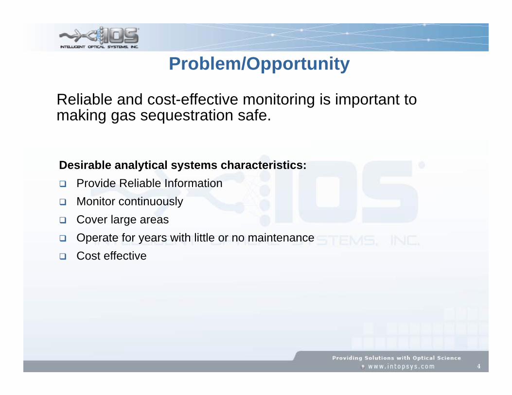
Problem/Opportunity
Reliable and cost-effective monitoring is important to making gas sequestration safe.
Desirable analytical systems characteristics: Provide Reliable Information Monitor continuously Cover large areas Operate for years with little or no maintenance Cost effective
5
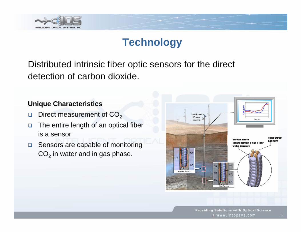
Technology
Distributed intrinsic fiber optic sensors for the directdetection of carbon dioxide.
Unique Characteristics Direct measurement of CO2
The entire length of an optical fiber is a sensor
Sensors are capable of monitoring CO2 in water and in gas phase.
6
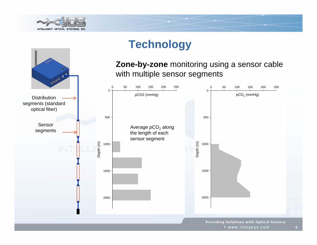
TechnologyZone-by-zone monitoring using a sensor cable with multiple sensor segments
pCO2 (mmHg)
0 50 100 150 200 250
Dep
th (m
)
0
500
1000
1500
2000
Average pCO2 along the length of each sensor segment
Sensor segments
pCO2 (mmHg)
0 50 100 150 200 250
Dep
th (m
)
0
500
1000
1500
2000
Distribution segments (standard
optical fiber)

7
A silica glass core fiber is coated with a polymer cladding containing a colorimetric indicator. Upon exposure of any segment of the fiber, the CO2diffuses into the cladding and changes color.
A light source is placed at one end of the fiber and a photodetector at the other end. The light transmitted through the fiber varies with the concentration of CO2.
(Left) Fiber structure of colorimetric distributed fiber optic sensors; (right) fiber optic CO2 sensor rolled onto a spool. Microscopic detail shows uncoated fiber, and fiber coated with the sensitive cladding.
Technology

8
CO2
CO2
Technology
The optical fiber must be exposed to the aqueous matrix (or gas)
Sensor cable incorporating multiple optical fiber sensors, which are exposed to the environment.

9
Phase I Development of advanced intrinsic fiber optic sensors and readout
(length up to 2,500 ft. and able to withstand corrosive liquids).
Sensor evaluation and demonstration in simulated subsurface conditions.
Pressure Temperature
Phase II
Subsurface sensor deployment and operation (in a 5,900 ft. deep well at up to 2,000 psi).
Phase III
Project Phases

10
The transmission of light through the fiber depends on the concentration of CO2, and isreversible.
Light at wavelengths far from the absorbance of the indicator dye are unaffected by thepresence of CO2, which enables the system to be self-referenced.
Time (s)
4000 6000 8000 10000 12000 14000
Sen
sor S
igna
l (co
unts
)
6000
8000
10000
12000
14000
0.0% CO2
1.0% CO2
6.0% CO2
Reference wavelength6.0%
1.0%
0.0%
6.0%
1.0%
0.0%
Testing at Ambient Pressure
11
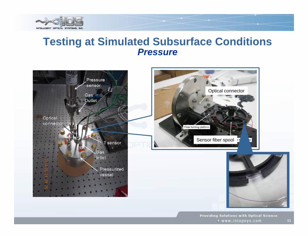
Testing at Simulated Subsurface ConditionsPressure
Sensor fiber spool
Optical connector

12
Gas cylinders
Pressurized vessel
Injection pumps
Control unit
Sensors immersed in water insidethe pressurized vessel
Injection pumps control gas flowand pressure
Gas cylinders with different CO2concentration (%) are used
Experiment Type 1: Constant CO2concentration and increasingpressure
Experiment Type 2: Constantpressure and varying CO2concentration
Testing at Simulated Subsurface ConditionsPressure

13
Time (s)
0 50 100 150 200 250
Sens
or S
igna
l (co
unts
)
0.0
2.0e+4
4.0e+4
6.0e+4
8.0e+4
1.0e+5
1.2e+5
1.4e+5
Increasing Total Pressure and pCO2
Increasing Total Pressure. Constant pCO2 (nitrogen)
P = 20 psipCO2= 0.2 psi
P = 50 psipCO2= 0.5 psi
P = 100 psipCO2= 1.0 psi
P = 200 psipCO2= 2.0 psi
P = 300 psipCO2= 3.0 psi
P = 20 psipCO2= 0.0 psi
P = 50 psipCO2= 0.0 psi
P = 100 psipCO2= 0.0 psi
P = 200 psipCO2= 0.0 psi
P = 300 psipCO2= 0.0 psi
Test 1: Nitrogen cylinder and increasing total pressure (black)Test 2: 1% CO2 in nitrogen cylinder and increasing total pressure (blue)
Testing at Simulated Subsurface ConditionsPressure

14
Progress – Simulated Subsurface ConditionsPressure
Test 1: Nitrogen cylinder and increasing total pressure (black)Test 2: 6% CO2 in nitrogen cylinder and increasing total pressure (green)
Time (s)
0 50 100 150 200 250 300
Sens
or S
igna
l (co
unts
)
0.0
5.0e+4
1.0e+5
1.5e+5
2.0e+5
2.5e+5
Increasing Total Pressure. Constant pCO2 (nitrogen)Increasing Total Pressure and pCO2 (at 6% v/v)
P = 20 psipCO2= 1.2 psi
P = 50 psipCO2= 3.0 psi
P = 100 psipCO2= 6.0 psi
P = 200 psipCO2= 12 psi
P = 300 psipCO2= 18 psi
P = 20 psipCO2= 0.0 psi
P = 50 psipCO2= 0.0 psi
P = 100 psipCO2= 0.0 psi
P = 200 psipCO2= 0.0 psi
P = 300 psipCO2= 0.0 psi
P = 20 psipCO2= 1.2 psi
15
Time (hours)
0.0 0.5 1.0 1.5 2.0 2.5
Sen
sor S
igna
l (co
unts
)
2.0e+4
4.0e+4
6.0e+4
8.0e+4
1.0e+5
1.2e+5
Pre
ssur
e (p
si)
0
500
1000
1500
2000
2500
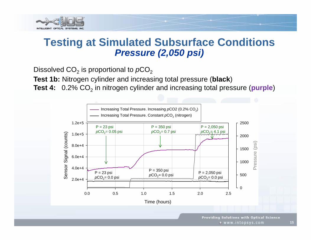
Increasing Total Pressure. Increasing pCO2 (0.2% CO2)Increasing Total Pressure. Constant pCO2 (nitrogen)
P = 23 psipCO2= 0.05 psi
P = 350 psipCO2= 0.7 psi
P = 2,050 psipCO2= 4.1 psi
P = 23 psipCO2= 0.0 psi
P = 350 psipCO2= 0.0 psi P = 2,050 psi
pCO2= 0.0 psi
Dissolved CO2 is proportional to pCO2
Test 1b: Nitrogen cylinder and increasing total pressure (black)Test 4: 0.2% CO2 in nitrogen cylinder and increasing total pressure (purple)
Testing at Simulated Subsurface ConditionsPressure (2,050 psi)

16
Time (hours)
4 5 6 7 8 9 20 21 22 23
Sen
sor S
igna
l (co
unts
)
2.0e+4
4.0e+4
6.0e+4
8.0e+4
1.0e+5
1.2e+5
Pre
ssur
e (p
si)
0
500
1000
1500
2000
2500
Dissolved CO2 is proportional to pCO214 to 8 h: Pressure set at 350 psi. Gas cylinders: N2 – 0.2% – 1% – 6% CO220 to 23 h: Pressure set at 2,050 psi. Gas cylinders: N2 – 0.2% – 1% – 6% CO2
Nitrogen
pCO2= 20 psiCO2 = 6%
pCO2= 3.5 psiCO2 = 1%
pCO2= 0.7 psiCO2 = 0.2%
pCO2= 4.1 psiCO2 = 0.2%
pCO2= 21 psiCO2 = 1%
Nitrogen
Testing at Simulated Subsurface ConditionsPressure
17
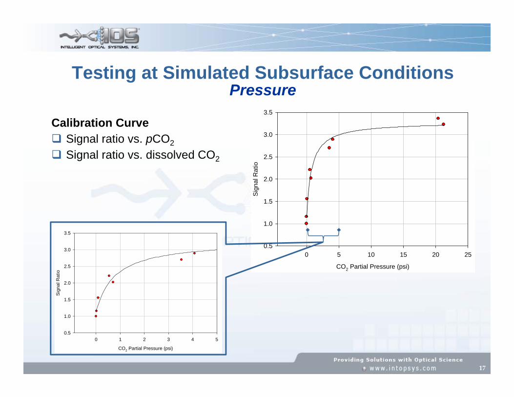
CO2 Partial Pressure (psi)
0 5 10 15 20 25S
igna
l Rat
io0.5
1.0
1.5
2.0
2.5
3.0
3.5
Calibration Curve Signal ratio vs. pCO2
Signal ratio vs. dissolved CO2
CO2 Partial Pressure (psi)
0 1 2 3 4 5
Sig
nal R
atio
0.5
1.0
1.5
2.0
2.5
3.0
3.5
Testing at Simulated Subsurface ConditionsPressure
18
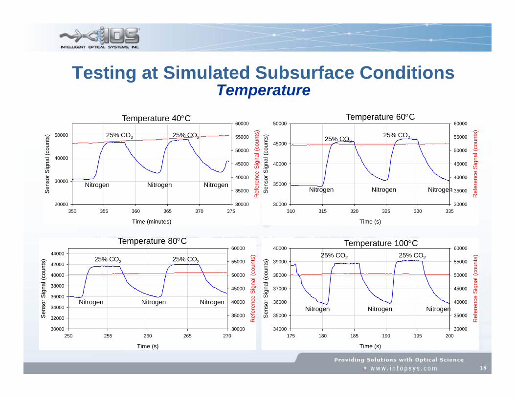
Testing at Simulated Subsurface ConditionsTemperature
Time (s)
310 315 320 325 330 335
Ref
eren
ce S
igna
l (co
unts
)
30000
35000
40000
45000
50000
55000
60000
Sen
sor S
igna
l (co
unts
)
30000
35000
40000
45000
50000
Time (minutes)
350 355 360 365 370 375
Ref
eren
ce S
igna
l (co
unts
)
30000
35000
40000
45000
50000
55000
60000
Sen
sor S
igna
l (co
unts
)
20000
30000
40000
50000
Temperature 40C
Nitrogen Nitrogen Nitrogen
25% CO2 25% CO2
Temperature 60C
Nitrogen Nitrogen Nitrogen
25% CO225% CO2
Time (s)
250 255 260 265 270
Ref
eren
ce S
igna
l (co
unts
)
30000
35000
40000
45000
50000
55000
60000
Sen
sor S
igna
l (co
unts
)
30000
32000
34000
36000
38000
40000
42000
44000
Temperature 80C
Nitrogen Nitrogen Nitrogen
25% CO2 25% CO2
Time (s)
175 180 185 190 195 200
Ref
eren
ce S
igna
l (co
unts
)
30000
35000
40000
45000
50000
55000
60000
Sen
sor S
igna
l (co
unts
)
34000
35000
36000
37000
38000
39000
40000Temperature 100C
Nitrogen Nitrogen Nitrogen
25% CO2 25% CO2

19
Progress – Simulated Subsurface ConditionsTemperature
Time (s)
110 115 120 125 130
Ref
eren
ce S
igna
l (co
unts
)
30000
35000
40000
45000
50000
55000
60000
Sen
sor S
igna
l (co
unts
)
34000
35000
36000
37000
38000
39000
40000Temperature 120C
Nitrogen Nitrogen Nitrogen
25% CO2 25% CO2
Time (s)
135 140 145 150
Ref
eren
ce S
igna
l (co
unts
)
52000
54000
56000
58000
60000
62000
64000
Sen
sor S
igna
l (co
unts
)
66000
68000
70000
72000
74000Temperature 140C
Nitrogen Nitrogen Nitrogen
25% CO2 25% CO2
Time (minutes)
10 15 20 25
Ref
eren
ce S
igna
l (co
unts
)
40000
42000
44000
46000
48000
50000
Sen
sor S
igna
l (co
unts
)
1.284e+51.286e+51.288e+51.290e+51.292e+51.294e+51.296e+51.298e+51.300e+51.302e+51.304e+5
Temperature 175C
Nitrogen Nitrogen Nitrogen
25% CO2 25% CO2

20
Time (minutes)
0 5 10 15 20
Nor
mal
ized
Sen
sor S
igna
l
0.9
1.0
1.1
1.2
1.3
1.4
1.5
1.6
1.7Temperature = 40 CTemperature = 60 CTemperature = 80 CTemperature = 100 CTemperature = 120 CTemperature = 140 CTemperature = 175 C
Demonstrated sensor operation up to 175°C Sensor aging is significantly accelerated at temperatures >140°C As expected, sensitivity decreases with temperature because the CO2 solubility
in the sensitive polymer decreases.
Progress – Simulated Subsurface ConditionsTemperature

21
Progress – Accelerated Degradation Tests
Stress Conditions High-power lighting Corrosive matrix (low pH and high salinity) Elevated water flow rate Highly biologically-contaminated matrix Temperature cycles.
We designed Accelerated Degradation Tests (ADT) based on theHighly Accelerated Life Test (HALT) methodology. The first objective is to collect information that allows us to
improve sensor lifetime The second objective is to quantitatively estimate the lifetime
of the fiber optic sensors.

22
Progress – Accelerated Degradation Tests
Sensor films covered with a protective, gas-permeable coating wereexposed to a highly biologically-contaminated matrix
The antimicrobial effect of three coating materials was measured The CO2-sensitive polymer was replaced with an oxygen-sensitive
polymer.
Oxygen sensitive film covered by protective cladding materials
Control in DI water
Highly colonized nutrient media
Samples exposed tocontinuous bacteria incubation

23
Progress – Accelerated Degradation Tests Sensor films covered with a protective, gas-permeable coating were
exposed to a highly biologically-contaminated matrix The CO2-sensitive polymer was replaced with an oxygen-sensitive
polymer Bacteria was allowed to grow on the polymer for several weeks The antimicrobial effect of three coating materials was measured by
measuring the oxygen consumption of the biological layer on thepolymer.
Time (minutes)
0 10 20 30 40 50 60
Oxy
gen
(mg/
L)
4.0
4.5
5.0
5.5
6.0
6.5
7.0
7.5
8.0DC 3140 Coating exposed to bacteriaDC3140 Coating in clean waterIOS 21-2 Coating exposed to bacteriaIOS 21-2 Coating in clean waterGE Coating exposed to bacteriaGE Coating in clean water

24
Progress – Accelerated Degradation Tests
Sensor fiber segments were exposed to elevated water flow rates forseveral months
Sensitivity to CO2 was measured periodically.
Fiber optic sensor prototypesExposed to continuous water flow
Water pump
Fiber optic sensor prototypesControl samples

25
Progress – Accelerated Degradation Tests
Sensor fiber segments were exposed to elevated water flow rates forseveral months
Sensitivity to CO2 was measured periodically.
Time (days)
0 25 50 75 100 125
Tran
s/Tr
ans
o (6%
Co2
)
1.0
1.2
1.4
1.6
1.8
2.0FlowNo Flow
Time (days)
0 25 50 75 100 125
Tran
s/Tr
ans0 (6
% C
O2)
1.0
1.1
1.2
1.3
1.4
1.5
FlowNo Flow
Fiber Type 1 Fiber Type 2

26
Progress – Accelerated Degradation Tests
Sensor fiber segments were exposed to ambient and elevatedtemperature cycles
Sensitivity was measured before and after each temperature cycle In parallel, sensor fiber segments were maintained at elevated
temperature and sensitivity was measured periodically.
Temperature Cycle A (n cycles)Cycle B (m cycles)
Temperature 2
Temperature 1
Temperature ST Test Test Test Test

27
Progress – Accelerated Degradation Tests
Sensor fiber segments were exposed to ambient and elevatedtemperature cycles.
Test Progress
Initial 70C C1 70C C2 70C C3 70C C4 70C C5 70C C6 70C C7 70C C8
Nor
mal
ized
Sen
sor S
igna
l (Se
nsiti
vity
)
0.0
0.2
0.4
0.6
0.8
1.0
1.2
1.4
1.6
1.8
2.0
0.0% CO2
1.0% CO2
6.0% CO2

28
Progress – Accelerated Degradation Tests
Sensor fiber segments were exposed to ambient and elevatedtemperature cycles.
Test Progress
Initial 70C C1 70C C2 70C C3 70C C4 70C C5 70C C6 70C C7 70C 10 70C C13 70C C16
Nor
mal
ized
Sen
sor S
igna
l (S
ensi
tivity
)
0.0
0.5
1.0
1.5
2.0
0.0% CO2
6.0% CO2
10.0% CO2

29
Progress – Accelerated Degradation Tests Sensor fiber segments were exposed to ambient and elevated
temperature cycles, and sensitivity was measured periodically (black) In parallel, sensor fiber segments were maintained at elevated
temperature and sensitivity was measured periodically (blue) Eight ADT cycles corresponded with 3 years/1,095 days of sensor
operation at constant temperature.
Thermal ADT Cycles
0 2 4 6 8
Sens
itivi
ty a
t 6%
CO
2
1.60
1.62
1.64
1.66
1.68
1.70
1.72
1.74
1.76
1.78
ADT study at 70C
Thermal ADT Cycles
0 2 4 6 8
Sens
itivi
ty a
t 6%
CO
2
1.60
1.62
1.64
1.66
1.68
1.70
1.72
1.74
1.76
1.78
Days at elevated temperature
0 10 20 30 40 50 60 70
ADT study at 70CContinuous Operation at 70C

30
Progress – Accelerated Degradation Tests Sensor fiber segments were exposed to ambient and elevated
temperature cycles, and sensitivity was measured periodically (black) In parallel, sensor fiber segments were maintained at elevated
temperature and sensitivity was measured periodically (blue) Eight ADT cycles corresponded with 3 years/1,095 days of sensor
operation at constant temperature.
Thermal ADT Cycles
0 2 4 6 8
Sens
itivi
ty a
t 6%
CO
2
1.60
1.62
1.64
1.66
1.68
1.70
1.72
1.74
1.76
1.78
Days at elevated temperature
0 200 400 600 800 1000
ADT study at 70CContinuous Operation at 70C

31
Progress – Accelerated Degradation Tests
Based on the ADT studies, and assuming linear decrease in sensitivityover time, we predict ~10 years of sensor service life.
Time (days)
0 10 20 30 40 50 60 70
Sens
itivi
ty a
t 6%
(96
ppm
) CO
2
1.0
1.2
1.4
1.6
1.8
2.0
Time (months)
0 12 24 36 48 60
Sens
itivi
ty a
t 6%
(96
ppm
) CO
2
1.0
1.2
1.4
1.6
1.8

32
Sensor Cable Fabrication and Deployment
Distribution segment
Modular cable includes: External strength member Distribution segments Sensor segments Connector protector Cable head
External member
Connector protector
Cable head
Sensor segments Final loop
connector

33
Sensor Cable Fabrication and Deployment
Distribution segment
Distribution segment includes eight standardoptical fibers: Four fibers connected to LEDs Four fibers connected to the photodetector.
Distribution cableLength: 1,600 m
Total Fiber: 12,800 m
Photodetector1 2 3 4
LEDs (Light Sources)
Distribution segment

34
Sensor Cable Fabrication and Deployment
Stainless steel tube (wire) Serves as support for sensor cable deployment Will be used during development for CO2
release.
Stainless steel tube spool
External strength member Stainless steel
tube spool
Sensor cable spool

35
Sensor Cable Fabrication and Deployment
Connector protector
Sensor segment & metallic tube
Distribution segment &
metallic tube
Optical connector
Connector protector Connects the stainless steel tube and the optical
cables Mechanically protects the optical connectors.

36
Sensor Cable Fabrication and Deployment
Final loop connector
Loop optical connector
Connector protector Connects the stainless steel tube and the optical
cables Mechanically protects the optical connectors.

37
Sensor Cable Fabrication and Deployment
Sensor segments Incorporate fiber optic sensors protected
mechanically but exposed to the aqueous (gas)matrix.
Sensor segments
CO2 fiber sensors
Fiber sensors
38
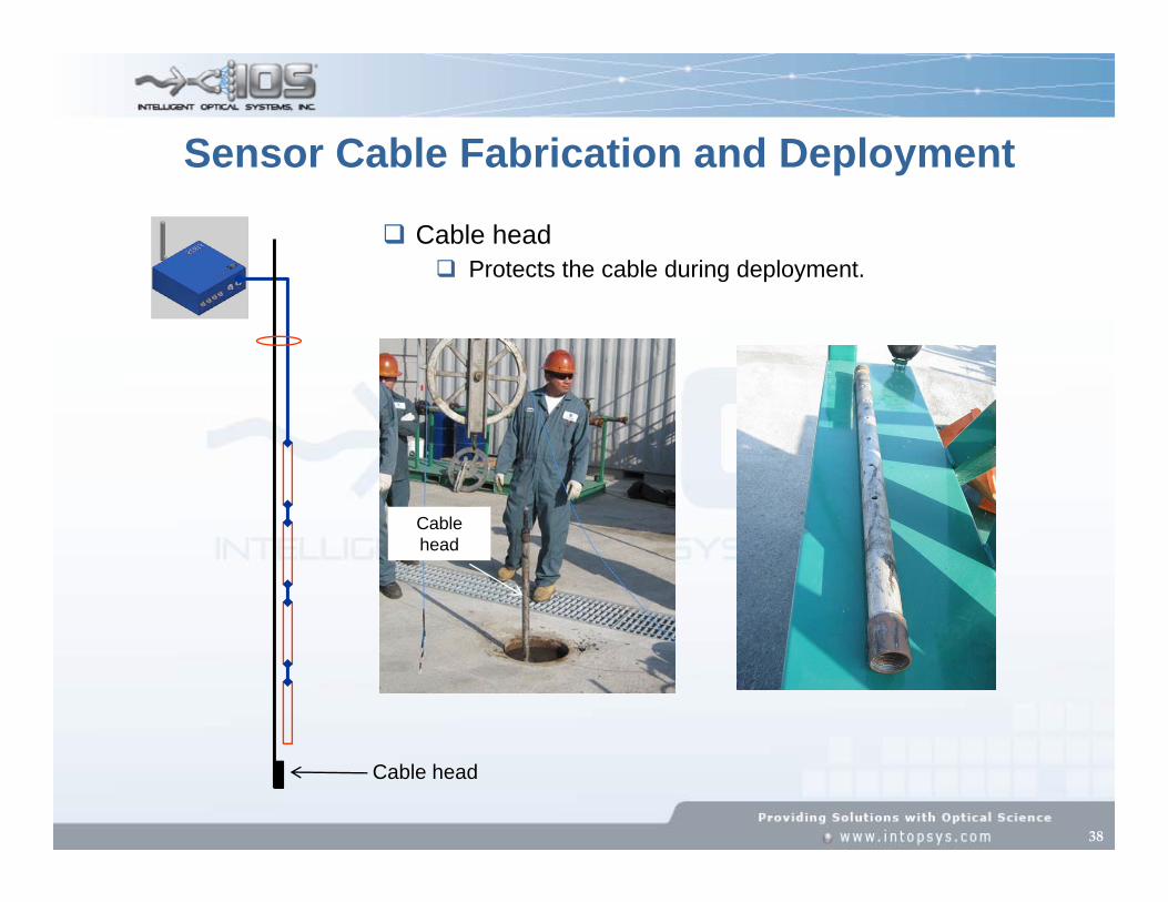
Sensor Cable Fabrication and Deployment
Cable head Protects the cable during deployment.
Cable head
Cable head
39
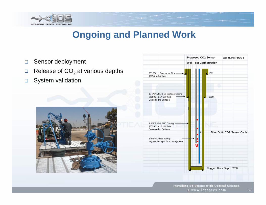
Sensor deployment Release of CO2 at various depths System validation.
Proposed CO2 Sensor Well Number DOE-1
Well Test Configuration
20" 65#, H Conductor Pipe 150'@150' in 26" hole
13 3/8" 54#, K-55 Surface Casing @1500' in 17 1/2" hole 1500'Cemented to Surface
9 5/8" 53.5#, N80 Casing@5350' in 12 1/4" holeCemented to Surface
Fiber Optic CO2 Sensor Cable
1/4in Stainless TubingAdjustable Depth for CO2 Injection
Plugged Back Depth 5250'
Ongoing and Planned Work

40
Demonstrated fiber optic sensor for CO2 monitoring in gas phase and for dissolved CO2 monitoring in aqueous matrices, capable of operating at elevated temperatures and pressure.
Conducted Accelerated Degradation Tests under a variety of stress conditions, and evaluated sensor limitations and stability.
Developed instrumentation demonstrating satisfactory performance while operating sensor cables 2 km in length. Calculations predict continued good performance for sensors 3 km and longer.
Designed and fabricated sensor cables. Developed and preliminarily tested sensor deployment system and
protocols. The system is being prepared for field deployment and testing by
controlled release of CO2 in a deep well.
Conclusions
41
Acknowledgments
GeoMechanics Technologies: (downhole sensor deployment)
Michael S. Bruno and Jeff Couture
NETL Department of Energy:Barbara Carney and Robie Lewis
Intelligent Optical Systems:Narciso Guzman, Straun Phillips and Sreekar Marpu