Embed Size (px)
Citation preview

University of Fribourg (Switzerland) Faculty of Economics and Social Science
Intraday Trading Activity on Financial Markets:
The Swiss Evidence
Thesis
Submitted to the Faculty of Economics and Social Science of the University of Fribourg (Switzerland)
in fulfillment of the requirements for the degree of Doctor of Economics and Social Science
by
Angelo Ranaldo
from Sementina (TI)
Accepted by the Faculty of Economics and Social Science on 17th February 2000 on the recommendation of
Professor Jacques Pasquier-Dorthe (First Reporter)
and
Professor Nabil Khoury (Second Reporter)
Fribourg, (Switzerland) 2000

«La Faculté des sciences économiques et sociales de l’université de Fribourg (Suisse) n’entend ni approuver, ni désapprouver les opinions émises dans une thèse: elles doivent être considérées comme propres à l’auteur (Décision du Conseil de Faculté du 23 janvier 1990».
Angelo Ranaldo was born in Sementina (Switzerland) on August 26, 1970. After attending scientific college in Bellinzona, he graduated in Business and Administration at the University L. Bocconi in Milan as «Dottore in Economia e Commercio». During his Ph.D., he worked at the University of Fribourg and attended the Gerzensee Ph.D. program run by the Swiss National Bank. Currently, he is a Visiting Scholar at the New York University, Stern School of Business as a post-doctorate researcher in the Finance Department.

5
ACKNOWLEDGMENTS
I carried out my Ph.D. thesis while working at the University of Fribourg (CH). During this period the chair of Finance was directed by Professor J.Pasquier-Dorthe and the working team consisted of Dr S. Gay Robin, Dr R. Häberle and later M. Ruffa and A. Vukic. I was very fortunate to be part of this team for two main reasons: first, because of the stimulating collaboration from which I learnt enormously and, secondly, because the team created an environment in which human aspects always took first place. In particular, I owe a debt to Prof. Pasquier-Dorthe who always showed immense sensitivity and understanding. He gave me the opportunity to attend the full Ph.D. program in Gerzensee (1997-8), he provided helpful feed-back on my work and, more important, he always gave importance to our human relationship. I am also very grateful to Sophie Gay Robin for her friendship and her useful advice.
I also thank all the people who made helpful suggestions related to my Ph.D. thesis. In particular, I would like to acknowledge Prof. N. Khoury who undertook to supervise my dissertation. I also thank Prof. P. Deschamps (University of Fribourg), Prof. Robert Engle (UCSD), Prof. Joel Hasbrouck (NYU), Prof. Bo Honoré (Princeton University) and Prof. C. Gouriéroux (CREST) and many colleagues at the University of Fribourg such as C. De Gottardi, F. Giorgetti, M.J. Redondo, Dr M. Sabooglu and B. Schmolck. I am extremely grateful to the Swiss Stock Exchange, in particular to J. Spillmann and S. Wick, who graciously provided the dataset.
I want also to express my gratitude to my family and to all those who gave me moral support. First of all I want to thank my partner, Karin, who is the main source of my sentiments and commitments. I will never thank her enough for her love for me. I am also especially indebted to my mother who provided continuous and generous attention. When I think of these two and of all my good friends I recognize my boundless fortune. As regards my friends I would not forget the “bohemian clan”, namely Chico, Diego, Fulvio, Gianlu, Gigi, Gio, Johnny, Marco, Max, Piffo, Rocco, and others such as Alberto, Andrea, Angelo, Michi, Mario and Omar. A final thought is reserved for the memory of my grandfather Rocco to whom this work is dedicated.

6
7
CONTENTS
ACKNOWLEDGMENTS. 5
CONTENTS 7
LIST OF ABREVIATIONS 9
LIST OF TABLES 13
0. INTRODUCTION 15
0.0 Abstract 17
0.1 Market Structures 18
0.2 Microstructure Models 21
0.3 High-Frequency Data 25
1: INTRADAY MARKET LIQUIDITY 31
1.0. Abstract 33
1.1. Introduction 34
1.2. Description of the Market and Dataset. 37
1.3. Intraday Patterns 39
1.4. Determinants of Market Liquidity 49
1.5. Conclusion 63
1.6. Figures 65
1.7. Tables 69
1.8. Appendix 79
2: THE INFORMATION CONTENT OF ORDER VOLUMES 87
2.0. Abstract 89
2.1. Introduction 90
2.2. Background and Literature Review 92

Intraday Trading Activity on Financial Markets
8
2.3. Description of the Market and Dataset. 97
2.4 The Tick-By-Tick Relationships 99
2.5. A Tick-By-Tick Ordered Probit Model 104
2.6. Conclusion 110
2.7. Tables 113
2.8. Appendix 125
3: LEAD-LAG RELATIONSHIPS BETWEEN STOCKS AND OPTIONS 131
3.0. Abstract. 133
3.1. Introduction 134
3.2. Review of the Literature 136
3.3. Dataset, Market Structure and Methodology 142
3.4. Empirical Findings 147
3.5. Conclusion 155
3.6. Figures 157
3.7. Tables 159
4. CONCLUSIONS 165
4.1. Intraday Market Liquidity 167
4.2. The Information Content of Order Volumes 174
4.3. Lead-Lag Relationships between Stocks and Options 177
4.4. Research Agenda 181
5. REFERENCES 183
9
LIST OF ABREVIATIONS AC: Auto Correlation ACD: Auto Conditional Duration Adj. R-2: Adjusted R-squared AGEFI: a Newspaper of the French Swiss AIC: Akaike Information Criterion APT: Asset Pricing Theory ARCH: Auto Regressive Conditional Heteroskedasticity ARMA: Auto Regressive Moving Average CAPM: Capital Asset Pricing Model CATS: Computer Aiding Trading System CBOE: Chicago Board of Exchange D.-W. Stat.: Durbin-Watson Statistic FR: Flow Ratio GARCH: Generalized ARCH Log likel.: Logarithmic Likelihood LR: Liquidity Ratio LSE: London Stock Exchange NASDAQ: National Association of Securities Dealers Automated Quotations NYSE: New York Stock Exchange NZZ: Neue Zuercher Zeitung OR: Order Ratio OWAIT: the Waiting Time between the Time Arrival of Two Subsequent Orders PAC: Partial Auto Correlation Prob(F-s): Probability related to the F-Statistic PSE: Paris Stock Exchange

Intraday Trading Activity on Financial Markets
10
RBSVI: Ratio of Volume Imbalance between the Buy and the Sell Part of the Market RGINI: Ratio of the Gini Index RLRC: Ratio of the First Level of the Return Autocorrelation RS: Ratio of Bid-Ask Spread RTAV: Ratio of Trading Volume Average RTV: Ratio of Trading Volume RVR: Ratio of Returns Volatility S.D. dependent var.: Standard Deviation of Dependant Variable SEAQ: Stock Exchange Automated Quotation System S.E. of regr.: Standard Error of the Regression SMI: Swiss Market Index SOFFEX: Swiss Options and Financial Futures Exchange SPI: Swiss Performance Index SRETURN: Stock Return SSR: Sum of Squared Residuals SVOL: Cumulated Trading Volume on Stock Market SWAIT: the Mean of the Waiting Time between Subsequent Trades SWX: Swiss Stock Exchange TARCH: Threshold ARCH URVT: Ratio of Unexpected Trading Volume VAR: Vector Auto Regression VCALL: Cumulated Trading Volumes of Call Options VCP: Cumulated Trading Volumes of Call and Put Options
List of Abbreviations
11
VIMB: Order Volume Imbalance between the Buy and the Sell Part of the Market
VIMBAV: VIMB in Absolute Value
VPUT: Cumulated Trading Volumes of Options
VR: Variance Ratio
VT: Trading Volume
WT: Waiting Time between Subsequent Trades

12 13
LIST OF TABLES
Introduction Table 0.1: The Market Structures of the Main Stock Markets
in the World by Agency and Dealer Markets, by Continuous and Call Markets. 20
1: Intraday Market Liquidity
Table 1.1: The Pearson Correlation between Eight Liquidity Proxies 69
Table 1.2: Fifteen Swiss Stocks as Ranked by Different Liquidity Proxies 70
Table 1.3: An Estimation of Intraday Market Concentration 71 Table 1.4: Intraday Market Depth as Trading Volume 72 Table 1.5: Intraday Market Depth Estimated by Order Volume
Imbalance 73 Table 1.6: Time Dimension of Intraday Market Liquidity 74 Table 1.7: Tightness of Intraday Market liquidity 75 Table 1.8: Intraday Relationships between Spread and Trading
Volume 76 Table 1.9: Intraday Return Volatility 77 Appendix 1.1: Proxies of Intraday Market Liquidity 79 Appendix 1.2: The Gini Index 82 Appendix 1.3: Intraday Market Variables 83 Appendix 1.4: The Distribution of the Four Cases 85
2: The Information Content of Order Volumes
Table 2.1: Tick-by-Tick Relations between Volume Imbalances and Returns the Fifteen Swiss Stocks 113

Intraday Trading Activity on Financial Markets
14
Table 2.2: Tick-by-Tick Relationships between Order Volume Imbalances and the Waiting Time between Orders for the Fifteen Swiss Stocks 115
Table 2.3: Tick-by-Tick Relationships between Order Volume Imbalances and Returns over the Trading Day for the Novartis and the Nestle Stocks 117
Table 2.4: Tick-by-Tick Relationships between Order Volume Imbalances and Returns over the Trading Day for the UBS N and the Clariant Stocks 119
Table 2.5: Tick-by-tick Ordered Probit Model applied to Fifteen Swiss Stocks 121
Table 2.6: The Ordered Probit Model over the Trading Day: the Novartis Stock 123
Appendix 2.1: The Distribution of the Ten Intraday Events 125 Appendix 2.2: The Ordered Probit Model over the Trading Day:
the CS Stock 126 Appendix 2.3: The Ordered Probit Model over the Trading Day:
the Clariant Stock 128 3: Lead-Lag Relationships between Stocks and Options
Table 3.1: Intraday Relationships between Option and Stock Volumes 159
Table 3.2: Intraday Relationships between Call, Put and Stock Volumes 160
Table 3.3: Intraday Relationships between Option Volume and Waiting Time to Trade on the Stock Market 161
Table 3.4: Intraday Relationships between Call and Put Option Volumes, and Waiting Time to Trade on the Stock Market 162
Table 3.5: Intraday Relationships between Option Volumes and Stock Returns 163
Table 3.6: Granger Causality Test Results 164
15
Introduction

16
Introduction
17
Abstract
This study is a theoretical and empirical research on financial markets. In particular, we focus on microstructure theory and intraday empirical investigations, which are two of the most recent developments in Finance. The empirical analysis is based on a high-frequency dataset of Swiss stock and option markets. The importance of these research areas has several roots. Historically, since the beginning of the ‘80s a large number of financial markets around the world have been changing their structures and have become informatized. Practically, markets are more and more inter-linked and traders take intraday positions. The organization of the introduction is as follows. In Section 0.1 we try to describe the historical evolution and the main features of market structures. Section 0.2 is a survey of the microstructure literature while Section 0.3 emphasizes the most important outlines of the research areas based on high frequency data. In order to help the reader, along this introduction we will write in italic the original contributions presented in the other parts of this study.
Intraday Trading Activity on Financial Markets
18
0.1. MARKET STRUCTURES
The structure of a securities market refers to the systems, procedures and rules that determine how orders are handled and translated into trades and how transaction prices are set. From this point of view, the micro-foundation of financial analysis is enormously important. While much of economics is concerned with the trading of assets, market microstructure research focuses on the interaction between the mechanics of the trading process and its outcomes, with the specific goal of understanding how actual markets and market intermediaries behave (Easely and O’Hara, 1995). This focus allows researchers to pose applied questions regarding the performance of specific market structures, as well as more theoretical queries into the nature of price adjustment.
The preliminary task of this introduction is to briefly define the main features characterizing a financial market. Following the framework of Biais, Foucaoult and Hillon (1997) we shall use three principal criteria to classify the different typology of market structures: (1) the trading time, (2) the market agents, and (3) the trading place.
As regards trading time we distinguish between continuous versus call markets. A continuous market allows trades to be made at any time during a trading day that counterpart orders cross in price. In a call market, orders are batched for simultaneous execution at the points in time when the market is “called”, typically one or two calls for a stock in a working day (see Schwartz, 1988).
The second criterion refers to the type of market agent, that is an agency market or a dealer market. In the former, public orders go to a broker’s broker, who matches them with other public orders. Market professionals do not participate in trading in an agency market (for instance the United States over-the-counter market). In the latter, a dealer, unlike a broker, participates in trades as a principal, not as an agent. Thus, a dealer satisfies a public order by buying or selling for his or her own inventory and public traders do not trade directly with each other, but rather with a dealer who serves as intermediary (for example the Tokyo Stock Exchange). A similar way to distinguish between agency or dealer market consists in describing the market typology through the price formation process. We define an order driven market as a trading system where the buy
Introduction
19
and the sell order are directly matched while a price driven market is an exchange system where the traders must trade with a market-maker who continuously provides a bid and an ask price (see, for example, the NASDAQ and the SEAQ). In some markets the market maker is the monopolist for a given asset, as on the NYSE where he is called “the specialist”, while in many other cases market makers are in competition.
The third criterion is based on the trading space, which can be centralized or fragmented. A trading system is spatially fragmented if orders can be routed through different markets. There are many types of market fragmentation: order flow may be fragmented for exchange listed issues and issues may be cross-listed (listed on more than one exchange); some orders are handled differently from other orders (for instance small orders are routed to immediate execution or large block trades are negotiated off-board in an upstairs market).
Much electronic equipment has been introduced in recent years. Since Toronto became the first stock exchange to computerize its execution system in 1977, electronic trading has been instituted in Tokyo (1982), Paris (1986), Australia (1990), Germany (1991), Israel (1991) Mexico (1993), Switzerland (1995), and elsewhere around the globe. In computerized trading, orders electronically entered in the system are executed, not by the market maker or the traders themselves, but by the computer.
In Table 0.1 we provide a summary of the possible market structures by combining the main features, namely agency/auction versus dealer markets and continuous versus call markets. We also specify whether the market has electronic trading.
At the present time, an enormous variety of market structures are available. Hence there is an open discussion regarding which is the best market structure. For instance, Handa and Schwartz (1996) raise the question of how best to supply liquidity to a security market. They also provide a useful comparison between the generic alternatives, namely agency/auction environments and the dealer market, the call market and continuous trading. Some other papers stress the advantages of an order-driven market in a general view, as in Handa, Schwartz and Tiwari (1998), and in order to provide liquidity, as in Varnholt (1996 and 1997).

Intraday Trading Activity on Financial Markets
20
Table 0.1: The market structures of the main stock markets in the world by agency and dealer markets, by continuous and call
markets.
Agency/Auction Markets
Dealer markets
Continuous Markets Continuous Markets U.S., NYSE * Toronto, CATS Tokyo, CORES Paris, CAC Germany, IBIS Switzerland, SWX Instinet
U.S. Nasdaq London, SEAQ Switzerland, SOFFEX
Call Markets Call Markets Opening Procedure ** NYSE Open Arizona Stock Exchange, Bolsa Mexicana, Taiwan Stock Exchange,
Not Available
* This is not an Electronic Trading ** For Most Electronic Markets
However it is necessary to set up theoretical models and
empirical analysis in order to improve our understanding in terms of different market structures. The following parts of this work analyze in detail the intraday functioning of the Swiss stock and option markets. We provide a new contribution to understanding how an order-driven market behaves and to what extent it differs from a price-driven market. We also examine the intraday dynamics in the Swiss stock and option markets. In Europe little work addresses this topic and none of it looks at Swiss markets.
Introduction
21
0.2. MICROSTRUCTURE MODELS To claim that different trading mechanisms affect the
behavior of prices is not a new idea. Nevertheless, to put the emphasis on the specificity of the market structures provides a new theoretical approach and stimulates empirical studies. From the theoretical point of view, in the past, the Walrasian market simplification in which auctioneers automatically clear was sufficiently convincing, even if there was some criticism as to the level of abstraction (e.g. Desmetz, 1968). The first main simplification is related to the first welfare theorem of the Arrow-Debreu model that assumes that all economic agents have the same information, or, at least, all agents are identically uncertain. If agents are asymmetrically informed, however, there are a number of fundamental changes in the economic analysis. First, agents’ behavior may reveal information. This behavior will be reflected in market variables such as prices and, hence, these market variables will reflect information not initially known to all agents. Thus, if there is asymmetric information, then economic variables have an information content and strategic behavior by agents becomes a factor.
Another simplification that stimulates the development of the microstructure literature is that theoretical security-valuation models neglect the effect of market structure on asset prices. Consider for example the CAP Model or the Asset Pricing Theory. These theories address the risk and the return dimensions of security, but ignore considerations like trading costs, information costs and transaction uncertainty, all of which are properties of an illiquid market and, more important, all of which are factors that can cause the failure of market efficiency.
However, our aim here is to summarize the theoretical basis of the microstructure models, so we will not present a historical list of models in this domain or establish the linkage between the microstructure and other domains of financial theory or economics. The theoretical foundation of the microstructure research stems from inventory, sequential trading game and asymmetric information theory. Three of the most influential original works are Demsetz (1968), Grossman (1976) and Garman (1976). Demsetz (1968) analyzed the nature of bid and ask prices and, in so doing, began the

Intraday Trading Activity on Financial Markets
22
micro-foundation of financial studies on market structure. Grossman (1976) studied the asymmetric information between traders using the theoretical concept of equilibrium with rational expectations. The title of Garman’s paper (1976) is extremely significant: “Market Microstructure”. Garman focused on price dynamics according to the nature of the order flow and the market clearing procedure. Other contributions followed.
Grossman (1976) provided an elegant model based on the idea that if informed traders correctly anticipate price movement then non-informed traders can infer the private information and, as a consequence, equilibrium including all information is always possible. Grossman and Stiglitz (1980) went further, inserting into the model informational costs for informed traders. The model shows that no traders are interested in buying private information given that the gain of an informed trader is less than a non-informed one. Indeed the equilibrium price will not involve all information and the hypothesis of strong market efficiency is not respected. In both models informed traders do not strategically consider the fact that they disclose information through their trading activity, in another words, they behave in perfect competition.
More recent models have relaxed this hypothesis, as in Kyle (1985) and Laffont and Maskin (1990), even if both these assume that the informed trader is a monopolist. However the former presents at least two important consequences: (1) when informed traders are aware that their trading activity can be interpreted by other agents as a signal then the price informational efficiency is weaker, and (2) asymmetric information slightly determines market liquidity. The latter and Gale and Hellwig’s model (1989) prove that when informed agents do not act competitively then multiple market equilibria are possible1.
The more recent microstructure models were typically based on the following hypotheses: first, there are only two assets, i.e. a risky and a risk free asset, in a one period economy, second, economic agents have an exponential utility function. Obviously
1 In a multiperiod context, Khoury and Perrakis (1998) focus on the role of asymmetric information on Spot and Futures markets. In an endowment of random private information, one of the main implications is that the basis conveys information about future spot prices but biased estimation occurs.
Introduction
23
these two assumptions are very restrictive and numerous contributions attempt to relax these statements2. Third, there are two kinds of traders: informed and non-informed. The former has complete or partial information about the value of the risk asset at the end of the period. Obviously the agents face a maximization problem of expected utility conditional on information distribution and the equilibrium price is determined by the equilibrium on the assets market that, in turn, is determined by the rational expectations of the agents. The fourth hypothesis is the assumption of rational expectations. The more realistic models typically assume that agents behave in a non-competitive way. At this point, an important distinction among the various models concerns the nature of the asset price dynamic. The first possibility occurs when the supply of the risky asset is observable by all traders and if its equilibrium price is transformable into the equivalent value of risk free asset. In this case non-informed traders can perfectly deduce private information by means of the equilibrium price. The second possibility is represented by a stochastic and non-observable supply of risk asset and therefore the impossibility for the non-informed traders to retrieve the signal. In this context, a price movement is considered a noise process which may be due to an exogenous source, i.e. some “noise” or “liquidity traders” needing money or acting irrationally3, or may be due to an endogenous source, i.e. some informed traders who maximize expected utility according to their endowments4.
Notice that the models are prevalently based on two types of dealer market structures: (1) a call market as in Grossman (1976), Grossman and Stiglitz (1980), Kyle (1989) and Laffont and Maskin (1990) or (2) a sequential trade model of a price driven market as in Glosten and Milgrom (1985), Kyle (1985), Easley and O’Hara (1987 and 1992) and Glosten (1989). Glosten (1994) shows the robustness 2 See, for instance, Khoury and Perrakis (1999) for the multiperiodicity combined with exponential functions. 3 Notice that the behavior of the liquidity traders changes according to the hypothesis. In Admati and Pfleiderer (1988) and Foster and Viswanathan (1993) liquidity traders may have discretion over when they trade. 4 The models typically suppose that: (1) the stochastic supply of the risk asset follows a normal distribution with mean zero and given variance, and (2) both value of the risk asset and risk free asset are random variables independently distributed.

Intraday Trading Activity on Financial Markets
24
of an electronic market with an open limit order book while Madhavan (1992) compares the price formation process in a price driven market and in an order driven market. Foucault (1993) and Parlour (1998) focus on a dynamic limit order market providing a game theory model of price formation.
Our work frequently refers to the microstructure of an order-driven market with a limit order book. For this reason the most important reference will be the model of Glosten (1994). For instance, in Chapter 1 we examine this model and we provide an empirical model based on the Glosten’s framework. However we will compare our theoretical and empirical results with the entire microstructure literature.
Introduction
25
0.3. HIGH FREQUENCY DATA The recent development of high frequency databases, i.e. a
dataset containing tick-by-tick data on trades and/or orders, allows for empirical investigations of a wide range of issues in the financial markets. The paper of Goodhart and O’Hara (1997) provides a straightforward summary of this literature pointing out how the advent of high frequency data bases contribute to shedding new light on model estimations and on econometric methods of market microstructure.
Some of the most important reasons why sets of high frequency data become available to researchers are based to (1) the low cost of data collection at the present, (2) wider and wider use of electronic technology in the financial markets, and (3) increased ability and capacity to manage and analyze very large dataset.
The NYSE is the most extensively studied financial market, but its particular characteristic makes it difficult to generalize the results to other markets. In fact, the NYSE is essentially a hybrid market, combining batch and continuous trading, a dealing floor and an “upstairs” mechanism for arranging block traders, a limit order book and a designated monopoly specialist. These particular features do not allow the generalization of empirical findings on the NYSE and new research is needed.
One of the most important topics of the high-frequency data deals with the market liquidity and intraday “seasonals”. Our work provides a new and a significant contribution in this research field. In Chapter One, for instance, we analyze the intraday dynamics of market liquidity by applying a new approach. Another important topic is the market reaction to large block trades. Seppi (1992) and Keim and Madhavan (1996), for instance, investigate the relation between price behavior and large block trades indicating fertile fields of research. In Chapter One, Two and Three we present original studies related to this research area. For instance, in contrast to the previous literature, in Chapter One we propose a method to estimate the intraday market concentration. In Chapter Two we study the tick behavior of order volume imbalances over the trading day while in Chapter Three we investigate the information content of option volume with respect to the intraday trading activity on the Swiss stock market.

Intraday Trading Activity on Financial Markets
26
An innovative contribution related to “high-frequency” studies is the change of the nature of trading time. While in traditional theory price and market components are typically observed at fixed time intervals, the more recent microstructure models (for example, Easley and O’Hara 1992, or Easley et al. 1996)5 and “high-frequency” studies stress the difference between calendar and operational time. Among others, Dacorogna et al. (1993) describe a model of time deformation for intraday movements of foreign exchange rates, Hausman and Lo (1990) specially examine the time between trades, and Ghysels and Jasiak (1994) provide a stochastic volatility model with the volatility equation evolving in an operational time scale. Another recent and promising research domain involving trading time analysis is represented by the application of duration models in tick-by-tick studies, as originally proposed by Engle and Russell with the ACD (Autoregressive Conditional Duration) model (1995) and by Ghysels, Gouriéroux and Jasiak (1997). In Chapter One we study the time dimension of intraday market liquidity. In Chapter Two we provide empirical evidence of the difference between calendar and transaction time. In Chapter Three we show that the trading speed on the stock market is related to the trading activity on the option market.
Most empirical studies with “high-frequency” data look at the time series of volatility, trading volume and spreads. Several researchers argue that all these time series follow a U-shaped or a J-shaped pattern, i.e. the highest point of these variables occurs at the opening of the trading day, they fall to lower levels during the midday period, and then rise again towards the close (among others, see Harris (1986) and Jain and Joh (1988)). The behavior of these variables is not easy to explain theoretically using the basic models related to threefold types of agents: the informed trader, the non-informed trader and the market maker. The introduction of a distinction between discretionary and non-discretionary uninformed traders partially overcomes this difficulty. If the uninformed or liquidity traders can choose discretionarily the time of their trades,
5 In the first microstructure models time is irrelevant, as in Kyle (1985) where market price is determined by the trading imbalance, or in Glosten and Milgrom (1985) where agents do not care about trading time and its information content.
Introduction
27
then they congregate in the periods when trading costs are low. This collective behavior increases market liquidity and also stimulates informed traders to trade in such periods in order to disguise better their private information. However, more information is revealed in such intervals, implying a positive relationship between volatility and volume (Admati and Pfleiderer (1988) and Foster and Viswanathan (1993)). Some other models go further in explaining the positive relation between volatility and spread, indicating that more volatility is associated with the revelation of more information, and thus the market becomes more uncertain and spreads widen (Foster and Viswanathan (1993) and Lee, Mucklow and Ready (1993)). The model of Brock and Kleidon (1992) exhaustively explains how the elasticity of the transaction demand involves the U-shaped pattern. The present study describes the intraday liquidity patterns on the Swiss stock and option markets. Among other purposes, we recognize to what extent intraday liquidity dynamics such as the volatility-volume and the volatility-spread relationships depends on private or public information. Furthermore, this study raises a question not yet investigated by the literature, namely whether an intraday pattern of market concentration exists and how intraday market concentration is related to market liquidity.
Another traditional topic in microstructure literature concerns the determinants of the spread. Just recently this topic has been analyzed using “high-frequency” data allowing a better understanding of the intraday behavior of bid ask spread. The first model dates back to Roll’s paper (1984) and is based on several strict hypotheses such as the homogeneous information of the agents, the independence of orders and no price occurring within the spread. Glosten (1987) eliminates the hypothesis of information homogeneity while the model of Stoll (1989) allows us to consider all three components of bid-ask spread, namely inventory, adverse selection and incentive costs6. A more realistic model was proposed
6 As described by Goodhart and O’Hara (1997), there are three main factors in the determination of spread. First, inventory carrying costs create incentives for market makers to use prices as a tool to control fluctuations in their inventory. Second, the existence of traders with private information, the adverse selection motive, implies that rational market makers adjust their beliefs, and hence prices, in response to the perceived information in the

Intraday Trading Activity on Financial Markets
28
by George, Kaul and Nimalendran (1993) who introduced the expectation of price movements showing that models excluding the time variation of price dynamic expectation produce biased results. While the models of Roll, Glosten, Stoll and George, Kaul and Nimalendran are based on a similar approach based on the autocovariance of price changes, Hasbrouck (1991 and 1993) provides a new method related to the variance decomposition7, in particular the variance of the equilibrium price changes and of the difference between transaction and equilibrium prices. The former variance serves to recognize the impact of information on prices, while private information has a permanent impact on the equilibrium price. The latter refers to other components of spreads, namely inventory costs. The empirical evidence of Hasbrouck’s analysis reveals that asymmetric information explains a large part of the volatility of the equilibrium price movements. A more sophisticated and general model was recently presented by Madhavan, Richardson and Roomans (1997). This model stems from a small number of hypotheses but at the same time it takes into account all of the components of bid ask spread: order time dependence, the possibility that the price occurs within the spread and the expectations of price movements. Using the generalized method of moments to estimate the market parameters, they consider five intraday time intervals composing the trading day. Among other results, this research shows that adverse selection costs are at the highest level at the opening and then decrease, while the other spread components have the opposite pattern. This last finding represents a new contribution to explaining U-shaped patterns. In Chapter One we also analyze the intraday dynamics of bid-ask spread as well as all the other components of market liquidity.
Another characteristic of “high-frequency” studies is the wide use of the GARCH to model the auto-correlation in the market volatility. The ARCH models (auto-regressive conditional heteroskedasticity models) were originally introduced by Engle (1982) and the GARCH models (generalized ARCH) by Bollerslev
order flow. Third, there are the other costs and the competitive conditions that influence the mark-up charged by the single market maker. 7 Hasbrouck uses the vector auto-regressive (VAR) analysis to solve his model.
Introduction
29
(1986). The latter author with Chou and Kroner (1992) provides an exhaustive explanation of the use of this model in finance. Kim and Kon (1994) compare different types of these models indicating that, among others, some approaches allow us to recognize the asymmetric (or leverage) effect of the conditional heteroskedasticity and, in particular, the Glosten, Jagannathan, and Runkle specification (1993), or Threshold-ARCH ( Zakoian (1990), Rabemananjara and Zakoian (1993) and Longin (1997)), is the most descriptive for individual stocks, while the exponential model as in Nelson (1991) is the more likely for indexes. Engle and Ng (1993) also compare TARCH and EGARCH models suggesting that the former is the best parametric model. In Chapter One and Three we apply these models but with some new contributions: (1) we analyze not only price volatility, as usual, but also volatility other market components, (2) our analysis is based on intraday data, and (3) the results contribute to shedding new light on previous outlines of the asymmetric impact of news (Engle and Ng (1993)).
Studies of inter-market relationships constitute a main area of research in the microstructure literature. The inter-linkage normally concerns different markets in terms of the type of asset traded (stocks versus options) and in terms of geographical diversity. Unlike studies of individual equity markets, a theory able to guide empirical analysis on this topic is not available, other than models such as in Back (1993). In any event, the efficient market hypothesis implies that mispricing and arbitrage opportunities between related markets should not exist. Hence lead-lag relationship between stock and option markets represents an opportunity to test market efficiency and to verify Black’s intuition (1975) on the greater attractiveness for an informed trader of the option market compared to the stock market because of the higher leverage available on the former. In the third part of this work we provide an exhaustive analysis of this literature and we investigate the inter-linkage existing between trading volume on option markets and a number of variables on the stock market, where the literature typically focuses on the relationship between option and stock returns.

30
31
CHAPTER 1:
Intraday Market Liquidity

32
Chapter 1: Intraday Market Liquidity
33
Abstract
Chapter 1 has four main objectives. First, we gauge intraday market liquidity through commonly used measures and some new proxies. Comparing these measures, we find their intraday patterns and their main features. Second, we detect and gauge the intraday pattern of market concentration. Third, since the rationale of this paper is that market liquidity is a complex and multidimensional concept, we investigate more deeply each component of intraday market liquidity. Among other things, our results show that the proxy of intraday market tightness follows a ARCH model while measures of intraday market depth follow a TARCH model. We also analyze the time dimension of intraday market liquidity, i.e. the waiting time between subsequent trades, and we complete our empirical findings by taking returns volatility into consideration. For each variable we examine its relationship with all other intraday liquidity components, intraday market concentration and the correlation of one-lagged returns. Finally, we propose a way to characterize intraday market activity in terms of four different situations, namely when either (discretionary) liquidity traders or informed traders prevail, and whether a price revision is occurring or not. Each market component is studied using this approach.

Intraday Trading Activities on Financial Markets
34
1.1. INTRODUCTION
This Chapter addresses the following questions: (1) do the available measures of liquidity provide the same estimation of market liquidity; (2) does an intraday pattern of market concentration exist; (3) how do the different components of intraday market liquidity behave during the day, and how are they related to each other; (4) how do the different components of intraday market liquidity behave if market features change, namely if transactions are carried out in the context of price revision, or in a context characterized by homogeneous or heterogeneous information.
The empirical analysis is based on order and transaction data from the Swiss Stock Exchange (SWX), which is an order driven electronic market without market makers. The data includes information on the most actively traded stocks. It contains the best bid and ask prices and their corresponding order volumes at all times, as well as the corresponding transaction data. It is therefore possible to reconstitute the best bid and ask orders that immediately precede a transaction.
First of all, we characterize the intraday patterns of the stock market through the commonly used measures of stock liquidity: cumulated traded volumes, returns, waiting time between subsequent trades, bid-ask spread, intraday liquidity ratio, intraday variance ratio. For each liquidity proxy, we discuss the resulting shapes. These six measures of liquidity are compared with two other indicators, namely a flow ratio, which represents the short term mean number of shares traded in CHF divided by the waiting time between subsequent trades, and an order ratio, based on the order volume imbalances. On the one hand, we analyze the divergent behavior of these indicators and on the other hand, we study the correlation between each stock and the equity market as a whole. To do this, we calculate an aggregate Index containing all 15 stocks available for this study. This Index includes 15 of the 23 equities constituting the Swiss Market Index (SMI). It is then assumed that this Index can approximate the behavior of the market as a whole.
Our second objective is to study intraday market concentration through the statistical concentration ratio known as the Gini Index. Our intent is (1) to know whether the market
Chapter 1: Intraday Market Liquidity
35
concentration behavior expressed by the size of traded volumes follows some recurrent feature and therefore if it is possible to detect a more particular type of trader, for instance an institutional one, within the intraday pattern of market concentration, (2) to obtain an intraday proxy of market concentration which can stand as an explanatory variable to analyze the different components of intraday market liquidity.
In addition, as a third objective, this paper examines independently the dimensions of intraday market liquidity. The rationale of this study is that market liquidity is a complex and multidimensional concept, and for this reason research oriented to a unique indicator is misleading. Accordingly, we decompose market liquidity into depth, tightness and resiliency (Kyle, 1985) as well as the time dimension. In particular, we take cumulated trading volume and volume imbalances between buy and sell counterparts as market depth proxies, bid-ask spread as market tightness proxy, and waiting time between subsequent trades for the time domain. We also consider volatility of returns given its sensitivity to market information. All these variables are studied in relation to each other and to two other intraday market features, namely volume size concentration and correlation of lagged returns during the period under analysis. Since intraday patterns exist, the data must be adjusted for intraday seasonality. We therefore transform each half-hour of data into a logarithmic ratio with the half-hour data of the specific day as the numerator, and the value of the normal intraday pattern during this half-hour as the denominator.
The final objective of this Chapter is to analyze the behavior of the intraday liquidity components with respect to different market situations. This approach is based on Glosten model (1994) which predicts that the severity of adverse selection is related to marginal price function and to trade size. Following this model, we use dummy variables to detect four possible cases. Each case indicates the more likely market situation, namely if a market revision is occurring, or that if a period is characterized by the presence of liquidity traders or informed traders.
The organization of this Chapter is as follows. In Section 1.2 we illustrate the most important aspects concerning the data and the structure of the Swiss Stock Market. In Section 1.3 we conduct a
Intraday Trading Activities on Financial Markets
36
preliminary exploration of the intraday market patterns of liquidity measures and of the concentration Index. In Section 1.4 we take into account the different components of intraday market liquidity and then we present the empirical findings. Section 1.5 concludes Chapter 1. The Figures of this Chapter are depicted in Sections 1.6 while the Tables and the Appendix are in Section 1.7 and 1.8, respectively.
Chapter 1: Intraday Market Liquidity
37
1.2. DESCRIPTION OF THE MARKET AND DATASET
The Swiss exchange system has undergone a fundamental change in the nineties. At the end of 1990, there were seven stock exchanges in Switzerland, alongside Soffex. In 1992, the Swiss Electronic Exchange project began and August 2, 1996 saw the launch of electronic trading in Swiss equities and derivatives, followed by bonds on August 16, 1996. This was the world's first fully integrated stock market trading system covering the entire spectrum from trade order through to settlement (SWX 1996 a). Indeed the Swiss Stock Market has become a computerized limit order market in which trading occurs continuously from 10 a.m. to 4.30 p.m.1 This is one of three exchange periods when "regular trading" occurs. The other two are the "pre-opening, from 6 to 10 a.m. for equities current trading day and 4.30 to 10 p.m. for the next trading day, and "opening", from 9.30 to 10 a.m. The mechanism for entering an order is as follows: first, investors place their exchange orders with their bank; second, the order is fed into the bank's order processing system by the investment consultant, forwarded to the trader and verified or entered directly by the trader into the trading system, and from there transmitted to the exchange system; finally the exchange system acknowledges receipt of the order marking it with a time stamp and checking its technical validity. It is important to underline that there are no market makers or floor traders with special obligations, such as maintaining a fair and orderly market or differential access to trading opportunities in the market, as in the Paris Bourse (see Biais, Hillion, and Spatt 1995). So, adverse selection problems as in Rock (1990) are insignificant.
Before matching, orders on each side of the order book are organized in price-time priority, regardless of which matching procedure is being executed (SWX 1996b)2. Obviously, orders can be placed at best (Market Order) or with the limit price (Limit Order). Two other order types are the Hidden Order and the Fill or Kill Order. The former corresponds to an order above 200,000 CHF, 1 In 1998 the regular trading was set from 9 a.m. to 5 p.m. 2 The price-time priority rule consists in ordering the order book as follows: best price to worst price (where Market Orders are followed by Limit Order); then, within price, first in to last in.

Intraday Trading Activities on Financial Markets
38
which may be traded outside the market but must be announced within a half-hour. The latter is an order that must be completely matched in order to create a trade. The electronic transmission of an order usually takes less than a few seconds.
Our data set3 contains the history of trades and orders of 15 stocks4 in the Swiss Exchange, for March and April 1997. For each stock, the data set reports tick-by-tick data concerning trades: price, execution time (to a hundredth of a second) and the quantity exchanged, and orders: buy and sell price, cumulated volumes related to the best buy and sell price, and order book insertion time of each order. Indeed, this period is equal to 41 trading days including approximately 500,000 million data as regards trades and the related observations of orders. All the information in our data set is available to market participants in real time. For the simultaneous trades we calculate the cumulated trading volume and mean price. Then we subdivide the trading day into 39 periods of 10 minutes for the first part of our study, and into 13 periods of a half-hour, for the second part.
3 This data set was graciously provided by the Swiss Stock Exchange in Zurich. 4 All 15 firms have not undergone an extraordinary change or transformation during the sample period (NZZ archives March and April 1997).
Chapter 1: Intraday Market Liquidity
39
1.3. INTRADAY PATTERNS A. Measures of intraday market liquidity
Several authors have tried to define market liquidity, but its interpretation still causes some problems. The root of the problem lies in the multidimensional nature of liquidity, as emphasized in Amihud and Mendelson (1986), Grossman and Miller (1988) and Kugler and Stephan (1997). A usual approach consists in breaking up liquidity into three components: tightness, depth and resiliency (Kyle, 1985; Bernstein, 1987; Hasbrouck and Schwartz, 1988). That will be our main approach in Section 1.4. From another point of view, the complex nature of the market liquidity concept is indicated by the tension between liquidity - a market in which we can buy and sell promptly with minimal impact on the price of a stock - and efficiency - a market in which prices move rapidly to reflect all new information as it flows in the marketplace (Bernstein, 1987). However, liquidity is reflected by the ability to make even large trades rather quickly and with a reduced impact on market price. Therefore the liquidity concept seems to show itself through the behavior of at least three market features: volumes, waiting time and price movements. Indeed, we take into account cumulated trading volumes, the mean value of the waiting times between subsequent trades and intraday returns. All these proxies are calculated on period of 10 minutes. See Appendix 1.1 for the mathematical expression of these proxies.
Even if volumes5 are a standard measure for estimating interday and intraday liquidity patterns (e.g. Admati and Pfleiderer, 5 Intraday volumes and return patterns were originally studied by Harris (1986), who found that there are systematic intraday return patterns which are common to all of the weekdays, i.e. returns are large at the beginning and at the end of the trading day. Jain and Joh (1988) showed significant differences across trading hours of the day. Brock and Kleidon (1992) examined the effect of periodic stock market closure on transaction demand and volume of trade, and consequently bid and ask prices. Foster and Viswanathan (1993) also studied intraday trading volumes, return volatility and adverse selection costs. Their tests indicate that all these market components are higher during the first half-hour of the day.

Intraday Trading Activities on Financial Markets
40
1988) and more precisely market depth, this measure insufficiently reflects market impact through price reaction and the importance of the different sizes of trades, because numerous small trades and a large single trade are considered the same. Furthermore Jones et al. (1994) emphasizes how number of transactions instead of average trade size has to be considered as a better proxy of market activity6.
The waiting times to trade are a more recent interest in intraday financial studies. While works such as Easley and O'Hara (1992) and Easley et al. (1996) provide theoretical models emphasizing the time domain of trades, others such as Gouriéroux et al. (1997) present econometric support endowed by empirical findings. In our study we examine the waiting times between subsequent trades calculating its mean value at 10-minute intervals (see Appendix 1.1). As in Lippman and McCall (1986), this measure defines liquidity in terms of the time until an asset is exchanged for money. Although this estimator informs on the frequency of transactions and on the trader's waits, it fails to recognize depth, breadth and resiliency of the market for an asset. As we will see later, waiting time trading can be seen as an intensity proxy of market activity, but its information content changes according to the market situation.
Besides the bid-ask spread (e.g. Amihud and Mendelson, 1986), another common liquidity proxy is the liquidity ratio, LR (e.g. Cooper et al., 1985; Kluger and Stephan, 1997). This measure, which relates the number or value of shares traded during a brief time interval to the absolute value of the percentage price change over the interval, is based on the notion that more liquid stocks can absorb more trading volume without large changes in price. We propose to use LR as an intraday liquidity proxy with two versions (see Appendix 1.1). The former considers the trading volume as whole while the latter emphasizes the difference between stock's capitalization and the number of equities owned by the firm. We take into account both LR proxies since we want to verify whether the two variants have a different impact when we rank assets according to the liquidity level (see Table 1.2). The major limit of LR is its lack
6 However, Brennan and Subrahmanyam (1998) find a positive relation between the average trade size and market liquidity
Chapter 1: Intraday Market Liquidity
41
of time dimension, i.e. the length of time necessary to trade7. Another problem may be the ambiguous short period reaction of LR when news causes prices and volumes to vary. Normally, a high liquidity ratio represents high market liquidity, but if prices adjust too slowly, a large trading volume is necessary. In this case, a high LR could be associated with a less efficient market. Moreover, a practical problem arises when very brief periods are used and therefore the probability that the price changes are different from zero decreases.
The variance ratio (VR) corresponds to the difference between the volatility over a very short period of 10 minutes, σ2
BP, and the volatility over a longer period of 1 day, σ2
LP (see Appendix 1.1). Hasbrouck and Schwartz (1988) initially proposed this measure both as liquidity and an efficiency market proxy. We propose VR as an intraday liquidity proxy indicating the relation between volatility of returns on a very short period of 10 minutes and daily volatility.
We finally introduce two other liquidity proxies: (1) a Flow Ratio (FR), based on the flow of volumes in Swiss francs traded each second, and (2) a ratio based on the bid/ask volume imbalances divided by cumulated volume traded during the same brief period. Taking the absolute value of the numerator, we do not take into account the direction of the difference. Lee et al (1993) and Engle and Lange (1997) present a similar liquidity proxy, but their indicators consider only the numerator of our proxy. Nevertheless we add traded volumes as denominator allowing a direct comparison across stocks and adjusting the liquidity measure to the market depth. B. Patterns of intraday market liquidity
Over the last decade several studies of the intraday pattern have been carried out and typically the empirical findings identified the U-shaped pattern. Admati and Pfleiderer (1988, p.3) wrote, for instance, that "the U-shaped pattern of average volume of shares, namely, the heavy trading in the beginning and the end of the day 7 Since price changes are involved in this liquidity ratio, discreteness constitutes another limit.

Intraday Trading Activities on Financial Markets
42
and the relatively light trading in the middle of the day, is very typical and has been documented in a number of studies". Our first goal is to verify whether the Swiss stock exchange follows a U-shaped pattern (e.g. Harris (1986), Jain and Joh (1988), Brock and Kleidon (1992) and Foster and Viswanathan (1993)) and for all the liquidity proxies previously presented.
To this end, we calculate these proxies for each stock and then construct a total Index containing all 15 stocks, which correspond to more than 94 % and more than 73 % of the total market values of SMI and SPI, respectively8. Figure 1.1 shows the graphical representations of the 8 liquidity proxies estimated for the Index. As we can see in Figure 1.1, all liquidity measures, including volatility returns, show: - A strong liquidity level at the beginning of the trading day,
reaching the absolute morning maximum between 10.10 and 10.30 a.m.;
- A decreasing liquidity pattern during the morning (10.30 until 12.10 a.m.), except the brief period beginning at 11.40 until 11.50 a.m.;
- A deep and long liquidity fall during the midday break (12.10 a.m. until 2.20 p.m.), however proxies more sensitive to the difference between bid and ask quotes show a persistent activity (see Return, OR, VR and Spread during 12.40-50 a.m. and 1.40-50 p.m.);
- A sharp resumption after the midday break (2.20 p.m.); - An evident liquidity slow down around 3.30 p.m., followed by
an immediate resumption 10 minutes later; - An intense rise of market liquidity around the closing time
reaching the absolute afternoon maximum in the last 10 minutes of the trading day (4.30 p.m.).
Our empirical findings on all liquidity indicators also show a sort of J-shaped curve, or rather that (1) the maximum of the morning is reached a few minutes after the opening, (2) the moments of lowest activity are concentrated during the lunch break (1.00 until
8 See Appendix 1.2 for more detailed explanations.
Chapter 1: Intraday Market Liquidity
43
1.20 p.m.) and (3) the absolute maximum occurs during the last few minutes of the trading day. Nevertheless, while all morning periods follow a smoothed negative plot, the afternoon part of the trading day indicates two temporary peaks. The first one occurs after lunch time (2.20-30 p.m.) and its effect persists for a half-hour. The second one coincides with the open time of US markets and it is preceded by an evident activity interruption. After US markets opening, the activity intensifies with the mean level reaching the absolute maximum at the end of the trading day.
We also observe that the return pattern is exactly correlated with trading volume behavior9. The only two features that distinguish the return pattern are that (1) the trading day begins with the highest level of the morning period, and (2) the lunch break begins almost 20 minutes or a half hour sooner with respect to the volumes.
Our results on intraday liquidity ratio, LR, show that it also works as an intraday liquidity proxy and that LR is highly correlated with all the other intraday liquidity measures. With respect to cumulated trading volumes, LR indicates the lunch break begins slightly later. This is not the same for intraday variance ratio, VR, which is more similar to features of return pattern and is most sensitive to the resumption of trading activity after the lunch break.
9 Even though the Swiss Stock Exchange differs from other stock markets on account of its two afternoon peaks, our findings are consistent with those of other studies, such as that of Stoll and Whaley (1990), which shows that returns and trading volume in the last part of the trading day are substantially higher than normal, or that of Lockwood and Linn (1990) who observed that return volatility falls from the opening hour until early afternoon and rises thereafter, and is significantly greater for intraday versus overnight periods. We can also link our results to those of McInish and Wood (1990) who showed that returns and number of shares traded have a U-shaped pattern when plotted against time of trading confirming that NYSE patterns also hold for the Toronto Stock Exchange. Other positive comparisons can be made with respect to research on options markets (Skeikh and Ronn, 1994) and studies on spillover effects between NYSE and the London Stock Exchange (LSE) (Susmel and Engle, 1994) both indicating a U-shaped volatility return patterns.

Intraday Trading Activities on Financial Markets
44
As with trading volume and volatility of returns, the microstructure literature has given a great deal of attention to bid ask spread 10. By contrast to McInish and Wood (1992) and in agreement with Brock and Kleidon (1992), our results show a clear positive relation between spread and trading volume. Thus we cannot accept the hypothesis that "there is an inverse relationship between spreads and trading activity" (McInish and Wood, 1992, p. 754). At the same time, we refute the predictions of current information based models such as those of Admati and Pfleiderer (1988).
Demos and Goodhart (1996) focused instead on the interaction between the frequency of market quotations, bid-ask spread and volatility in the foreign exchange market. Our results are also consistent with Demos and Goodhart's findings on at least two aspects: (1) the bid ask spread increases when market activity rises; (2) at the opening of European markets, European spreads widen. Our results confirm the former point showing a positive correlation between the spread and all the other liquidity proxies. The latter fact is also evident in our empirical findings and it is replicated at the opening time of US markets suggesting that Brock and Kleidon's argument can also explain the liquidity reaction of SWX when US markets open. We finally notice that our findings in an order-driven market confirm that the intraday behavior of the spread appears to be fundamentally different according to market structure, as suggested by Chan et al. (1995).
Order volumes were studied in a recent paper of Biais et al. (1995) on the Paris Bourse, but they did not define a concrete liquidity measure based on order flow. Engle and Lange (1997) found that the volume imbalances between the buy and sell sides of
10 Looking at intraday research, Brock and Kleidon (1992) clearly show wider spreads at the beginning and at the end of the day. The authors show that transaction demand at the opening and closing times is greater and less elastic than at other times of the trading day. As a result, a market maker such as a NYSE specialist may effectively use discriminate pricing by charging higher prices at these periods of peak demand. Their predictions of periodic demand with high volume and concurrent wide spreads are consistent with empirical evidence, while the predictions of current information based models are not. McInish and Wood (1992), Lee et al. (1993) and Chan et al. (1995) found a similar U-shape.
Chapter 1: Intraday Market Liquidity
45
the market are positively related with volume, but less than proportionally, and negatively related with number of transactions, expected volatility and spreads. Our empirical findings are consistent with Engle and Lange's outlines, but the fact that order ratio is highly and negatively related to all liquidity proxies indicates that volume imbalances between the buy and sell sides of the market must be more than proportionally related to traded volumes. Lee et al (1993) also found a negative relationship between volume imbalances and spread.
Our findings reveal in the first place that all liquidity proxies indicate that Swiss intraday liquidity patterns do not precisely follow a U-shape (as, among others, in Jain and Joh, 1988; McInish and Wood, 1990) nor a M-shape (as for the Paris Bourse in Gouriéroux et al., 1997). The Swiss stock exchange seems to show a U-shaped pattern only during the morning and the last half-hour of the trading day. Nevertheless, we note that not all the different proxies show a uniformly decreasing liquidity morning curve starting from the beginning of the trading day, in fact trading volumes, liquidity ratio and order ratio show the maximum liquidity occurrence of the morning between 10.10 and 10.20 a.m.
The most characteristic feature of the Swiss trading day is the three peaks during the afternoon (around 2.20 p.m., around 3.30 p.m. and just before the closing time). The first one is a peculiar feature found only in the Swiss and the German intradaily liquidity patterns (for the German market, see Röder (1996), Röder and Bamberg (1996) and Kirchner and Schlag (1998))11. This can be explained by three major facts. First, the lunch break ends. Second, the adjustment of Swiss and international traders’ positions on SWX in anticipation of US markets orientation on the basis of the US stock markets pre-opening as well as the US option markets opening, and
11 In Germany there is a complex market structure: the most liquid stocks are traded on several parallel markets with different features (floor or computer trading, dissimilar mechanism of price determination and different trading time). Moreover the German floor market has three batch auctions per day. The cited papers deal with a restricted number of liquidity proxies, namely the volatility and the average number of transactions; nevertheless they separately show that during the afternoon the activity on the computer trading system (IBIS) increases around 2.40 p.m. and 3.30 p.m.

Intraday Trading Activities on Financial Markets
46
the interpretation of news related to US markets. In fact, according to Becker, Finnerty and Friedman (1995), this is the moment when the main part of US macro news is released. Third, there is an important linkage between the Swiss and the German markets. The large number of dually listed securities on the Swiss and the German markets corroborates this explanation12. The second peak corresponds to the analogue afternoon peak of the Paris Bourse (Gouriéroux et al., 1997) and the German market (Röder, 1996; Kirchner and Schlag, 1998)13, 14. The third peak during the closing time evokes the U-shaped pattern. Hence it seems evident that the intraday liquidity pattern on the Swiss market follows a triple-U-shape.
Secondly, our findings also reveal that the status of asset liquidity may vary according to the liquidity proxy we use. Even if the different liquidity proxies are highly correlated (Table 1.1), in Table 1.2 we notice that the status of a single share may diverge completely: for instance, Roche is the least liquid in terms of cumulated trading volume and the most liquid in terms of the variance ratio. Nevertheless some similarity is also evident. For example, assets of Novartis, Roche, Nestlé and UBS N are ranked in the six first most liquid assets according to LR1, spread, FR and WT criteria, or that Ciba is present in the six most liquid positions on 6 out of 9 criteria. It is also interesting to note that the two versions of liquidity ratios in Table 1.2 present very different results. This suggests that a measure of market liquidity based on trading volume that neglects the actual free floating volumes may be misleading.
12 This remark is also noteworthy for the French and UK markets. According to the numerous dually listed French stocks on the UK exchange, an analogous feature seems to characterize the French intraday pattern. In fact, this could explain why the empirical findings indicate a M-shape (Gouriéroux et al., 1997). 13 The Pagano model (1989), which predicts trade concentration on some markets, may explain the liquidity rise on the Swiss market after the US markets open time. 14 The Pagano model (1989), which predicts trade concentration on some markets, may explain the liquidity rise on the Swiss market after the US markets open time.
Chapter 1: Intraday Market Liquidity
47
C. Intraday Market Concentration
One market aspect that may be extremely useful in providing an explanation of market liquidity is market concentration estimated by the distribution of traded volume size. As emphasized by Spiegel and Subrahmanyam (1995, p. 336), "(liquidity) measure depends not only on contemporaneous inventory and volume, but also on the distribution of volume that is expected to arrive in the future".
For these reasons, we suggest analyzing intraday market concentration and estimating size volume concentration with the Gini Index (see Appendix 1.2 for the mathematical expression and for further details). This Index represents a general proxy of size volume concentration for each period of 10 minutes and hence it allows us to estimate to what extent a trading period is characterized by a small number of large size trades or rather by the predominance of trades with a homogenous size. In Table 1.3 and Figure 1.2 we have taken into account the Novartis asset, the most liquid equity on SWX according to several measures (see Table 1.2). We can see the difference between the two extreme Lorenz curves of the trading day, i.e. the less concentrated Lorenz curve corresponding to 4.10 until 4.20 p.m., the nearest to the bisector, and the most concentrated one occurring between 3.50 and 4.00 p.m.
We calculate the Gini Index for each trading period of 10 minutes and notice some interesting features (see Table 1.3). The Gini Index mean during the trading day is 0.662 and we have to wait until 10.30-40 a.m. before seeing a higher concentration level. The same lagged moment of traded volume concentration occurs after the NYSE opening time (3.30 p.m.). If we relate high concentration levels to institutional traders' arrival, we can interpret this result as a pause by discretionary liquidity traders (Admati and Pfleiderer, 1988; and Foster and Viswanathan, 1990) in order to go beyond the two moments of uncertainty. The most evident and intriguing result is the enormous concentration at 3.50 until 4.00 p.m. This confirms our previous interpretation related to the substantial dependence of the Swiss Stock Exchange on the US markets, whereby Swiss investors try to know the behavior of US markets before deciding on

Intraday Trading Activities on Financial Markets
48
institutional investments. This fact becomes even more interesting if we consider that the period of time corresponding to the highest concentration is preceded by another period with one of the lowest concentrations in the trading day (3.40-50 p.m.). We already know that during this period of high concentration, the market liquidity and volatility of returns are very high, too. Hence we can argue that, soon after a crucial moment of uncertainty, as the US markets open, traders on the Swiss market15 take rather speculative positions and afterwards liquidity follows.
The empirical findings on the Gini Index also detect a considerable concentration level during the lunch period, particularly at 12.30 until 12.50 a.m. and at 1.10 until 2.00 p.m. On this occasion, our results seem to contradict the intuition of models such as that of Admati and Pfleiderer (1988) in which discretionary liquidity traders prefer to trade when the market is "thick". In fact our findings clearly show the presence of large size trades even during less liquid periods of the trading day suggesting that traders could strategically use volumes to obtain market impact.
15 We should not believe that only Swiss traders are trading on the Swiss market. It is possible that foreign traders trade on the Swiss market either for speculative or hedging reasons.
Chapter 1: Intraday Market Liquidity
49
1.4. DETERMINANTS OF MARKET LIQUIDITY A. The model
In the previous section of this Chapter, our analysis reveals the existence of an intraday pattern on the SWX. The presence of an intraday pattern implies that a further investigation of intraday market liquidity should not take into account the current level of market liquidity but rather the logarithmic ratio between the current level and its normal value at that current moment. In other words, we must adjust the data for intraday seasonality. Appendix 1.3 provides more detailed explanations and the mathematical expressions of the adjustment for seasonalities. For this further study, we analyze only the Novartis stock and we divide the trading day into 13 half-hours and not into 39 ten minute periods. In fact, the half-hour is an intraday period sufficiently lasting (Hasbrouck, 1999) in order to detect (1) the dominant presence of a type of agent (informed or liquidity traders), and (2) if a price revision process or no price reorientation is occurring. Moreover, the half-hour separation always allows us to obtain a representative sample with at least 20-25 observations, even if an illiquidity period elapses.
Following the Glosten's model (1994), we use another tool to better recognize different intraday market situations. Glosten's model predicts that the severity of adverse selection is positively related to the marginal price function, and hence to returns, and to trading size16. In Admati and Pfleiderer (1988) informed traders try to trade at the same time that liquidity traders concentrate their trading. As a result, the terms of trade will reflect the increased level of informed trading as well, and this may conceivably drive out the liquidity traders. In Brennan and Subrahmanyam (1998) trade size is determined by both informational and strategic considerations. Among the others, average size is related to the precision of private information and the informational advantage of informed traders. In Easley and O'Hara (1987) informed traders are free to choose the
16 Models based on market maker’s structure also predict that probability of information-based trading is lower when high volumes are traded (e.g. Easley et al 1996)

Intraday Trading Activities on Financial Markets
50
size of trading volumes and they choose the large-sized trades. Hence we labeled all half-hour periods as follows:
Case 1: both current level of trading volume size and current level of return volatility are higher than the normal level. During this period information asymmetry between traders is more likely, therefore informed traders may be present.
Case 2: while current level of trading volume size is higher than the normal level, return volatility is lower than normal. Homogeneous opinion and information are prevalent and, therefore, it is more likely that liquidity traders are present. Because of average of volume size, agents may be discretionary liquidity traders such as institutional investors.
Case 3: while current level of return volatility is higher than the normal level, trading volume size is comparatively low. During this period a price revision is occurring. The price reorientation may be due to (1) public information arrivals, and (2) a wider diffusion of private information.
Case 4: both current level of trading volume size and current level of return volatility are lower than the normal level. Liquidity traders dominate market activity17.
To detect these four cases we used the logarithmic ratio of average size of traded volumes, labeled as RTAV, and the logarithmic ratio of return volatility, labeled as RVR (see Appendix 1.3). When RTAV and RVR are positive, both ratios inform us that the current value is higher than the normal level estimated over a period of two months. We consequently used dummy variables in order to recognize the different cases.
Looking at the reasons why intraday price changes, we can sketch three possible explanations for such changes. First, a market impact caused by a liquidity trader leads to high volume and possible price change followed by a reversal. This is the case where the presence of (discretionary) liquidity traders is more likely, see Case 2 and 4. Second, a news arrival brings a high accumulation of trading volumes and a well-defined price reorientation. This situation corresponds to Case 3. Third, asymmetric information becomes more
17 To see the distribution of the four cases, see Appendix 1.4.
Chapter 1: Intraday Market Liquidity
51
accessible for the public and it becomes easier to get or interpret some private information. This situation is captured again by Case 3, where agents trade temporarily with small-sized transactions putting into motion a price revision expressed, for example, by a correlated lagged returns. In the case of severe asymmetric information (Case 1) informed traders are sufficiently few in number. If the asset is sufficiently liquid and if the insider information allows sufficient trading time to be profitable, agents can hide avoiding price and volume impact.
As you can see in Appendix 1.3, all variables are adjusted for intraday seasonalities. The data for cumulated volume becomes a ratio between current cumulated traded volumes and normal level of cumulated traded volumes, labeled RTV18. Following the same process, we calculate the ratio between current and normal levels of waiting time between subsequent trades, RWT, spread, RS, volume imbalances between buy and sell market sides, RBSVI and the Gini Index, RGINI. A particular consideration has to be given to the variable named RLCR. This acronym indicates the ratio between current and normal lagged correlation returns. In practice, we calculate the coefficient of correlation of one-lagged returns during each half-hour period (see Appendix 1.3). Considering the mean over two months for each of the 13 half-hour periods, we estimate the normal value of this coefficient. The information content of this ratio lies in the fact that if autocorrelation on intraday returns is higher than the level of the normal pattern then we suppose that a price revision based on public news or relative homogeneous information is occurring. McInish and Wood (1991) study autocorrelation of intraday returns and find that first-order autocorrelation follows a crudely U-shaped pattern, too. These results support our approach, which is to adjust data for intraday seasonality19,20.
18 See the mathematical expressions A.1.10 and A.1.11 and the other explanations in Appendix 1.1. 19 For all variables we verify the essential features of their time series, i.e. stationarity and normality and autocorrelation. Stationarity condition is verified through augmented Dickey-Fuller test and we find that all time series are largely above the MacKinnon’s critical value.

Intraday Trading Activities on Financial Markets
52
B. Intraday Market Depth In Terms Of Trading Volume
The first analysis concerns the actual market depth, i.e. cumulated traded volumes. Therefore we take RTV as the dependent variable and RBSVI, RWT, RGINI and RLRC as independent variables21.
Equation (2) presents the same variables as in equation (1) but it also includes dummy variables, dt,i where i=1,…, 4. The introduction of dummy variables allows us to analyze separately each of the four cases previously described. The sample and the frequency analysis of the four cases are in Appendix 1.4.
Table 1.4.A exhibits the results of the general case and shows that ratio of cumulated trading volume per half hour is positively related to (ratios of) returns volatility, order volume imbalances, volume concentration proxy, and negatively related to (ratios of) waiting time between subsequent trades and return autocorrelation proxy. Only the last variable can be rejected with a probability above 5% and under 10%. These relationships suggest that volume imbalances between counterparts, RBSVI, tends to be transformed into trading volume confirming that both indicators, namely RVT and RBSVI, inform on market depth. At the same time, waiting time between trades slightly increases when market depth decreases, while trading volumes decisively increase when market
20 All the correlograms show that autocorrelation (AC) has a large r1 and rt dies off geometrically with increasing lag, t. Partial correlation (PAC) is large only for the first and second lags. Indeed both AC and Durbin-Watson statistic suggest a first-order autoregressive model and PAC suggests a possible first-order moving average model. 21 Another important control concerns multicollinearity. In fact, there is a risk of collinear dependence between independent variables, therefore for each regression we carry out collinearity tests, namely the Variance Inflation Test, and we consequently take into account only the exempted variables.
(2) dRLRC
dRGINI dRWTdRBSVICRVTRVT
(1) RLRCRGINIRWTRBSVICRVTRVT
t
4
1iit,t
4
1iit,t
4
1iit,t
4
1iit,t1-tt
ttt1-tt1-tt
ε+η
+κ+γ+δ++α=
ε+η+κ+γ+δ++α=
∑
∑∑∑
=
===
Chapter 1: Intraday Market Liquidity
53
concentration improves. The former must be viewed as a proxy of trade frequency logically positively related to market depth. The latter means that a rise in market concentration brings a rise in the total amount of traded volumes. Trading volume also present one-lagged auto regressive level and auto regressive conditional heteroskedasticity22. More exactly, our variables follow the TARCH model (Zakoian (1990) and Glosten, Jagannathan, and Runkle (1993))23:
(3) d 21t1t
21t
21t
2−−−− βσ+γε+αε+ω=σ
In equation (3) we can see that the conditional variance of residuals includes two distinct one-lagged autoregression, ε2
t-1, depending on the sign of εt. By means of a dummy variable, dt-1, we recognize whether an asymmetric effect exists, i.e. if γ>0. The conditional variance also includes a constant, ω, and an AR(1), i.e. one-lagged conditional variance, σ2
t-1. If we interpret εt as news arrival (e.g. Engle and Ng, 1993), we can explain unexpected trading volumes as a reaction to a shock. Creating two ARCH components and putting a dummy variable on one of them for negative shocks, our result consistently shows that positive and negative ARCH components cancel each other out when a negative shock occurs. 22 After running ARMA models, the Fisher test and Akaike information criterion indicate that AR(1) has the biggest explanatory power. Nevertheless, the White Heteroskedasticity test indicates the presence of heteroskedasticity and the ARCH LM test clearly informs us that for several variables we should not accept the hypothesis which requires that all coefficients of the lagged squared residuals are zero. When required, we tried out all the plausible ARCH models and we found some GARCH(1,1) but also some TARCH(1,1) to be the most meaningful approaches. Using the likelihood ratio test and residual tests, we finally singled out the most powerful solution. After appropriate regressions, all the residuals present a time series with mean zero, and the Jarque-Bera statistic test indicates a normal distribution for residuals of the regressions where RWT and RRV are the dependent variables. 23 Some examples of use of TARCH models are in Rabemananjara and Zakoian (1993) and Longin (1997) while Engle and Ng (1993) provide a wide comparison of this model with respect the EGARCH and other ARCH processes.

Intraday Trading Activities on Financial Markets
54
This means that good news brings increasing traded volumes whereas bad news slows market activity reducing intraday market depth. Hence market reactions are not symmetrical, i.e. intraday market liquidity overreacts according to good news arrivals.
Table 1.4.B shows the results of four separate market situations (see equation 2) for which we retain only the variables with significant coefficients. Volume imbalance is significant only for Case 3 and Case 4 with a higher coefficient for Case 3. Trading volumes are better explained by order volume imbalances when a price revision is occurring (Case 3), since order volume imbalance is a proxy more sensitive to market disequilibrium. For the same reason, during periods of informed-based trades and liquidity-based trades, these two proxies of intraday market depth have different dynamics. We also see that waiting time and trading volume are always negatively related. The highest negative relationship concerns Case 2, i.e. when the presence of discretionary liquidity traders is more likely, and when trading volumes are constituted by large-sized trades. This may also indicate that uninformed traders could protect themselves by reducing trade frequency and, inversely, that trading waiting time could be used strategically by informed traders (an analogue result with respect to specialists control is found by Madhavan and Sofianos, 1998). The informed-based trading case is also the less sensitive to size volume concentration, i.e. the Gini ratio. In this case (Case 1) a rise in concentration level signals a more intense activity carried out by informed traders. The fact that there is not a positive relationship between concentration and market depth indicates how the informed traders successfully disguise their private information. The other three cases (Cases 2, 3 and 4) reveal a positive relationship. In Cases 3 and 4 the small and medium-small trading sizes are predominant, therefore a few large sized trades have a stronger market impact on market depth. Intraday market depth and correlation between lagged returns shows the highest negative relationship with respect to contexts of discretionary liquidity traders (Case 2) and periods of price revision (Case 3). A higher correlation means that the activity of price orientation is more intense and definite. Because of uncertainty, during these intraday periods discretionary liquidity agents do not trades and intraday market depth decreases.
Chapter 1: Intraday Market Liquidity
55
C. Intraday Market Depth Estimated by Order Volume Imbalances
Conceptually, we think that bid/ask volume imbalances may be a misleading market depth proxy, even if it seems to provide better information about the expected market capacity to absorb trading volumes. Lee and al. (1993) and Engle and Lange (1997) use this proxy to gauge market depth and they find similar results, namely a negative relationship between spread and volume imbalances. Nevertheless, this measure may confuse results. Actually, a low imbalance level could represent both a high market liquidity, when the difference between high buy and high sell volume cancel each other out, and an illiquid market, when buy and sell volumes are reduced. However, volume imbalance performs better if it is considered in relative terms, i.e. divided by its normal level, as we have done. The next analysis is based on equation (4) and (5) and results are shown in Table 1.5.A and 5B.
Again, the second equation (equation [5]), includes dummy variables allowing for the identification of the four different cases. Ratios of waiting time and Gini Index are similar to the other proxy of market depth, i.e. trading volume, even if the respective coefficients are smaller in absolute value. Moreover, we can see a negative and substantial relation between volume imbalance and spread, confirmed later by Table 1.7. These relationships are also incorporated into Table 1.5.B. The period of price revision (Case 3) presents the strongest negative relation between spread and volume imbalance supporting the idea of a wider spread during periods of high uncertainty. Case 2 also shows a large coefficient bearing out the significant role of discretionary liquidity traders. This idea is clearly confirmed by the correlation between lagged returns, which is negative for periods of discretionary liquidity trading (D2RLRC) and positive when price reorientation is occurring (D3RLRC). In the former period, the price revision brings uncertainty that induces
(5) dRGINI
dRWTdRSCRBSVIRBSVI
(4) RGINIRWTRSCRBSVIRBSVI
t
4
1iit,t
4
1iit,t
4
1iit,t1-tt
tttt1-tt
ε+κ
+γ+δ++α=
ε+κ+γ+δ++α=
∑
∑∑
=
==

Intraday Trading Activities on Financial Markets
56
discretionary liquidity to put off trades, therefore a high correlation between lagged returns implies a decrease in market depth. In the latter period, market depth expressed by the volume imbalance actually results from the activity of price revision. Notice that this is an important difference with respect to the relationship between trading volume and return correlation, see Table 1.4.B. This is another confirmation that order volume imbalances and trading volume are both market depth proxies, but with important differences. In particular, order volume imbalances are more sensitive to market disequilibrium. It is also important to underline that market concentration and trade frequency have a significant relationship with order volume imbalances only for the case of liquidity suppliers, Case 4. The conditional variance of residuals derived from regressions described by equation (4) and (5) presents an ARCH process. The time series of residuals reveals an autocorrelated stochastic process but, in contrast to trading volumes, we do not have here asymmetric components. D. The Time Dimension of Intraday Market Liquidity
Our objective in Table 1.6 is to analyze the time domain of intraday market liquidity; hence the waited time between subsequent trades is taken as the dependent variable. To do this, we carry out the following regressions:
The final result is that RWT follows an AR(1) while the conditional variance of the residuals a TARCH(1,1), as in equation (3). Again the residual component may be interpreted as an information arrival which causes a change in trade frequency24. For 24 The study presented in Chapter 3 analyzes the inter-linkage existing between the stock and option Swiss markets. We find similar results for the
(7) dRLRC
dRGINIdRVTCRWTRWT
(6) RLRCRGINIRVTCRWTRWT
t
4
1iit,t
4
1iit,t
4
1iit,t1-tt
tttt1-tt
ε+λ
+κ+β++α=
ε+λ+κ+β++α=
∑
∑∑
=
==
Chapter 1: Intraday Market Liquidity
57
this reason, it makes sense that conditional variance has a TARCH structure for which a negative shock simply eliminates the ARCH components leaving only the GARCH effect. This overreaction to good news is similar to the variance equation in Table 1.4.
Waiting time trading is negatively related to trading volume and return autocorrelation, but positively related to concentration Index of volume size. The relationship between trading volume and the trade frequency was already analyzed in Table 1.4. Here we confirm that the largest coefficients concern Cases 1 and 2. An original result is the following. Intraday market concentration slows down trade frequency, especially when market activity is dominated by liquidity suppliers (Cases 2 and 4) and when a price revision is occurring (Case 3), but not when information is spread heterogeneously (Case 1). A higher concentration level in Case 1 should indicate a wider presence of informed traders. Therefore these findings combined with the results in Table 1.4 suggest that agents with private information are capable to trade without altering the intraday liquidity extent both in terms of market depth and trade frequency. Moreover only Case 3 presents a significant relationship between return autocorrelation (RLRC) and trade frequency. The return autocorrelation signals to what extent the price revision is well oriented. Our result confirms that Case 3 is a context of price revision since a higher level of autocorrelation speeds trade activity. Finally, the spread shows positive relationships with periods of private information (Case 1) and periods of discretionary liquidity trading (Case2), but a negative one with respect to periods of price revision (Case 3). These outlines shed new light on the dynamics of trading time activity. These relationships indicate that the bid-ask spread is an efficient indicator of uncertainty when discretionary liquidity trades prevail and when informed traders can be present but not recognized. Nevertheless in a context of price revision a wider spread reflects a more rigid demand or supply (Brock and Kleidon, 1992). Hence, while in Cases 1 and 2 a positive coefficient was
lagged relationship between stock trade frequency and option trading volume. More precisely, our results show that (1) (option) trading volume are negatively related to (stock) waiting time trading, and (2) positive and negative shocks in the variance equation of residuals presents an asymmetric impact.

Intraday Trading Activities on Financial Markets
58
anticipated since a wider uncertainty decreases trade frequency, in Case 3 a wider spread indicates a definite price revision. E. The Tightness of Intraday Market Liquidity
In Table 1.7 we present a deeper analysis of spread, which may be interpreted as a market tightness proxy.
Our empirical findings help to understand the behavior of the bid-ask spread. Our results indicate that the spread ratio has an AR(1)-ARCH(1) model where spread widens when intraday market concentration rises, while spread decreases when volume imbalances decrease. Again, these relationships can be explained by thinking of volume imbalance as a market depth proxy and the Gini Index as a concentration volume size indicator.
It is interesting to see how these relationships vary according to each of the different cases in Table 1.7.B. We notice that the relation between volume imbalances and spread is significantly negative only when liquidity traders dominate trading activity, i.e. Cases 2 and 4 (see also Table 1.5.B). We also notice that the positive relation between market concentration and spread is due to Case 4. Periods of relatively higher concentration imply a relatively wider spread in a context of non-informed based trading activity. As in Tables 1.4.B and 1.6.B, the lack of a significant relationship between market concentration and spread in a context of private information (Case 1) shows to what extent informed traders are capable to disguise their activity.
In Table 1.8 we analyze the specific relationship between trading volume and spread. In particular, we carry out the following regressions:
(9) dRGINIdRBSVIRSRS
(8) RGINIRBSVIRSRS
t
4
1iit,t
4
1iit,t1-tt
tt1-tt
ε+δ+β+α=
ε+δ+β+α=
∑∑==
(11) dURVTRSRS
(10) dRVTRSRS
t
4
1iit,t1-tt
t
4
1iit,t1-tt
ε+β+α=
ε+β+α=
∑
∑
=
=
Chapter 1: Intraday Market Liquidity
59
Equation (10) investigates the spread/trading volume relation that was not taken into account before. Equation (11) refers instead to the relationship between the spread and the unexpected trading volume, URVTt 25. We begin with the analysis of equation (10).
The spread/trading volume relationship is one of the much-debated issues in intraday studies, which is basically empirically descried with a negative relationship. Through our approach we can see that this relation changes according to intraday market features. In Table 1.8.A the estimated coefficients are not significantly different from zero. However it is noteworthy that negative relationships occur only during informed-based trading periods (Case 1) or during price revision times (Case 3), but not when liquidity traders trade (Cases 2 and 4). McInish and Wood (1992) use as determinants of spread trading activity, risk level, amount of information and level of competition among specialists specifying that the first and the last are negatively related to the spread whereas the second and the third have a positive relationship. Our results help to understand that the determinants of spread have complex and dynamic behavior.
Furthermore, our findings can be related to the model of Easley and O'Hara (1992) that predicts that (1) spread depends on time between trades, with spread decreasing when this time increases, (2) (the lack of information and therefore) trade time affects the behavior of price, and (3) there exists a relationship between spreads and both normal and unexpected volumes. Besides the different market structures between the model of Easley and O'Hara and the SWX, we can successfully support the first and second predictions with the data represented in Tables 1.6.B and 1.9.B. The third prediction is corroborated by the results in Table 1.8.A and B. While Table 1.8.A shows the relationships between
25 The time series of unexpected trading volumes corresponds to the residuals of a regression in which trading volume is the explanatory and the dependent variable. In other words, we sought the most powerful regression in which trading volume predicts itself, that is an AR(1)-GARCH(1,1) process, and then we took into account the time series of the residuals, named URVTt.

Intraday Trading Activities on Financial Markets
60
spread and actual trading volumes, Table 1.8.B focus on unexpected trading volume.
If we interpret unexpected trading volume as a straight proxy of market uncertainty, a positive relationship between unexpected volume and spread carries weight when asymmetric information is more likely (Case 1) or when an intraday price revision occurs (Case 3). It is important to point out that for both cases that the relationship is negative when actual traded volumes are considered (Table 1.8.A). Since the bid/ask spread is positively related to uncertainty and actual trading volume is a proxy of market depth, then the more is severe the asymmetric information the more is negative the relationship between spread and volume. Nevertheless unexpected trading volume reflects the trading activity carried out by informed traders and hence it is positively related to the degree of information asymmetry as well as to the bid/ask spread.
As expected, inverse results are valid for the liquidity-based trades (Cases 2 and 4). In fact, a wider spread is also due to a less elastic demand or supply such as during intraday peaks of market liquidity. Hence we find a positive relationship between actual traded volume and spread in Cases 2 and 4. On the contrary, a negative correlation takes place when unexpected trading volumes are considered. In this case, liquidity traders interpret unexpected volumes as a signal of asymmetric information and, as a consequence, they may put off or suspend their trading activity. F. Intraday Returns Volatility
We finally investigate volatility of returns through equations (12) and (13).
(13) dRLRC
dRGINIdRBSVIdRSRRVRRV
(12) RLRCRGINIRBSVISRRRVRRV
t
4
1iit,t
4
1iit,t
4
1iit,t
4
1iit,t1-tt
ttttt1-tt
ε+λ
+κ+δ+β+α=
ε+λ+κ+δ+β+α=
∑
∑∑∑
=
===
Chapter 1: Intraday Market Liquidity
61
Our findings show that return volatility follows an AR(1)-GARCH(1,1) model. Notice that ratio of return volatility is similar to that of the intraday variance ratio (VR) previously used, nevertheless now the denominator is not the volatility of daily returns but rather corresponds to the mean of return volatility for the specific half hour in the long period investigated26.
Intraday return volatility is positively related to the bid-ask spread, to Gini Index and, to returns autocorrelation, and negatively related to volume imbalances (but with a relatively weak t-statistic). Return volatility slightly depends on traders' information. Spread and return volatility are positively related because both increase at asymmetric information times. In fact our empirical findings in Table 1.9.B show the highest coefficients in Cases 1 and 3. As we have already seen, volume imbalances may not be only a market depth proxy but it may also signal divergence between counterparts. Here it is interesting to note that the dummy variable related to RBSVI is positive for the context of informed and liquidity traders (Cases 1 and 4, respectively) while it is negative when a price revision occurs (Case 3). Hence for the former volume imbalance seems to be a more efficient proxy of intraday market depth while for the latter it constitutes a better indicator of market divergence among buy and sell counterparts. The Gini Index ratio is generally positively related to return volatility since a rise in volume size concentration implies several large-block transactions and, in turn, their market impacts imply temporary removals from efficient price and consequent higher return volatility.
Notice that market impact has a strong effect when market activity on liquidity trading with small-sized trades (Case 4). On the contrary, when a price revision elapses, the arrival of large-block trades and a rise in market concentration slow down the trading activity (Case 3). In Case 1, a rise in market concentration may reflect the presence of informed traders. These agents suitably avoid signaling their private information. Therefore they trade without impacting on prices.
26 This approach avoids the criticisms previously mentioned and takes into consideration the normal intraday pattern.

Intraday Trading Activities on Financial Markets
62
Finally, we observe an opposite sign for trade frequency in Cases 1 and 2. For the former, we have already noted that the context of private information seems to be very sensitive to trading time. Return volatility represents the intensity of market activity; hence a decrease in trading frequency signals that informed traders reduce their activity. By contrast, when it is more likely that liquidity suppliers trade (Case 2), a rise in return volatility corresponds to a wider uncertainty that slows down market activity since discretionary liquidity traders suspend their trades. Our results confirm those of previous papers that demonstrate that price movement is significantly positively related to trade size (e.g. Keim and Madhavan 1996), but also that speed of adjustment is a function of the size of the block (Holthausen et al. 1990). Our results show that this relation is much more evident when returns volatility is relatively low but average trade size is relatively high.
The final consideration regards the relationship between return autocorrelation and return volatility. Our results demonstrate that this relationship exists particularly in intraday periods of price revision.
Chapter 1: Intraday Market Liquidity
63
1.5. CONCLUSION
This Chapter dealt with the question of how to measure intraday market liquidity. To do this, we reviewed the commonly used liquidity proxies - namely trading volumes, returns, spread, and waiting time between trades - we adapted some proxies previously used as an interday liquidity measure - namely liquidity ratio and variance ratio - and we provided some new indicators, namely order ratio and flow ratio. We applied these proxies to 15 of the most liquid stocks traded on the Swiss Stock Exchange and we established an outline of the particular intraday liquidity pattern of the Swiss market. We then raised an issue not yet empirically studied in microstructure literature, namely whether an intraday pattern of market concentration exists, how to recognize it and to what extent it influences other market aspects.
In accordance with the idea that market liquidity is a multidimensional concept, we subdivided intraday liquidity into tightness, depth, resiliency and its time dimension. We analyzed each liquidity component with respect to each other and with respect to intraday market concentration, return volatility and correlation among lagged returns. Furthermore, we provided an original approach to detect the market context in which each liquidity component takes places. We identified four intraday market contexts: discretionary and non-discretionary liquidity trading, informed-based trading, and period of price revision. We then examined intraday liquidity components with respect to these different market contexts. Among other results, we find that intraday market depth estimated by trading volumes follows a AR(1)-TARCH(1,1) model and it is positively related to return volatility, volume imbalance between counterparts, market concentration, and negatively to waiting time between trades and to correlation of lagged returns, while if we gauge intraday market depth through order volume imbalances we find similar results but with other interesting implications. We also estimated intraday market tightness through the bid-ask spread and we find that spread is positively related to market concentration and negatively to volume imbalances.

Intraday Trading Activities on Financial Markets
64
The analysis of the time domain of intraday market liquidity shows that waiting time of trades follows an AR(1)-TARCH(1,1) model and is positively related to intraday market concentration and negatively to trading volumes.
The significant results provided by the TARCH model support the idea that the positive and negative shocks have differential effects on the conditional variance and therefore good and bad news have asymmetric impacts on the intraday market liquidity.
To complete our analysis, we examined intraday return volatility which presents a AR(1)-GARCH(1,1) process, positive relationship with volume imbalances, spread, market concentration and lagged correlation of returns.
It is important to underline that all these findings become even more intriguing when observed with respect to the four market contexts. For instance, our approach allows us to discover that spread and volumes are apparently negatively related, as the microstructure normally indicates. However a separate detection indicates that spread widens when trading volume increases only when liquidity trading is occurring, but an opposite relation is valid when information asymmetry and informed-based trades are more likely.
Finally, one of the main contributions of this paper was to reveal the features of the behavior of informed and liquidity traders. We documented that informed traders are able to trade in suitable intraday context keeping away from liquidity impact in terms of market depth and trade frequency. On the contrary, liquidity traders avoid intraday uncertainty. Discretionary liquidity traders put off their trades in front of signals of asymmetric information such as wider spreads, return autocorrelation and return volatility. Moreover, we clarified the dynamics of the different dimensions of intraday market liquidity when a price revision occurs.
Chapter 1 : Figures
65
1.6. FIGURES FIGURE 1.1: The intraday patterns of eight liquidity proxies. This Figure shows the intraday liquidity patterns of the Swiss market index based on 15 stocks calculated following the procedure described in Appendix 1.1. Each measure has been subtracted by its mean and then divided by its standard deviation. Hence the vertical axis presents the standardized extent of market liquidity. The horizontal axis corresponds to the time axis based on 39 periods of 10 minutes. Figure 1.1.A shows the intraday pattern of cumulated trading volumes (VT), return, and spread. Figure 1.1.B shows the intraday pattern of liquidity ratio (LR), variance ratio (VR) and flow ratio (FR). Figure 1.1.C represents the intraday pattern of order ratio (OR) and waiting time between trades (WT). Only WT and OR are negatively related to market liquidity and therefore the graphic in Figure 1.1.C is inverted.
Figure 1.1.A
-2-1.5
-1-0.5
00.5
11.5
22.5
33.5
1 5 9 13 17 21 25 29 33 37
Intraday Periods of 10 min.
Stan
dard
ized
Liq
uidi
ty
VTReturnSpread

Intraday Trading Activity on Financial Markets
66
Figure 1.1.B
Figure 1.1.C
-2-1.5
-1-0.5
00.5
11.5
22.5
33.5
1 4 7 10 13 16 19 22 25 28 31 34 37
Intraday Periods of 10 min.
Stan
dard
ized
Liq
uidi
ty
LRVRFR
-2-1.5
-1-0.5
00.5
11.5
22.5
33.5
1 5 9 13 17 21 25 29 33 37
Intraday Periods of 10 min.
Stan
dard
ized
Liq
uidi
ty
ORWT
Chapter 1 : Figures
67
FIGURE 1.2: Lorenz curves for size of trading volume of the Novartis stock for each period of 10 minutes constituting the trading day on SWX. On the horizontal axis there is the ratio of cumulated number of trades and the vertical axis corresponds to the ratio of cumulated traded volumes. Before cumulating traded volumes, we ordered traded volumes from the smallest size to the largest. See Appendix 1.2 for the mathematical expressions. The nearer the curve is to the horizontal axis, the more there is concentration of volume size during an intraday period. The nearest curve to the horizontal axis corresponds to the Lorenz curve for 3.50 until 4.00 p.m. while the nearest curves to the bisector correspond to the periods 4.10 - 20 p.m. and 3.30 – 40 p.m.
0
0.2
0.4
0.6
0.8
1
Hj0.0
75 0.15
0.225 0.3
0.375 0.4
50.5
25 0.60.6
75 0.75
0.825 0.9
0.975
Cumulated Number of Trades (H)
Cum
ulat
ed T
radi
ng
Vol
ume
(C)

68
Chapter 1 : Tables
69
1.7. TABLES TABLE 1.1: The Pearson Correlation between eight liquidity proxies. This Table exhibits the correlations among the 8 intraday liquidity proxies defined in Appendix 1.1. The calculation is based on the Swiss market Index estimated from 15 stocks. All correlations are significant at the 0.01 level (two-tailed). The acronyms indicate: TV trading volumes cumulated within 10 minutes, VR the variance ratio, LR1 the liquidity ratio relating cumulated trading volumes and price changes in absolute value within 10 minutes, FR the flow ratio, OR the order ratio, Return mean of returns, and WT the waiting time between subsequent trades.
TV VR LR1 FR OR Return Spread WT
TV 1 0.949 0.973 0.943 -0.849 0.966 0.766 -0.823
VR 0.949 1 0.883 0.9 -0.818 0.984 0.746 -0.745
LR1 0.973 0.883 1 0.916 -0.834 0.914 0.697 -0.856
FR 0.943 0.9 0.916 1 -0.69 0.893 0.835 -0.673
OR -0.849 -0.818 -0.834 -0.69 1 -0.861 -0.482 0.886
Return 0.966 0.984 0.914 0.893 -0.861 1 0.734 -0.811
Spread 0.766 0.746 0.697 0.835 -0.482 0.734 1 -0.399
WT -0.823 -0.745 -0.856 -0.673 0.886 -0.811 -0.399 1

Intraday Trading Activity on Financial Markets
70
TABLE 1.2: Fifteen Swiss stocks as ranked by different liquidity proxies. The acronyms indicate: TV trading volumes cumulated within 10 minutes, VR the variance ratio, LR1 the liquidity ratio relating cumulated trading volumes and price changes in absolute value within 10 minutes, LR2 is like LR1 but it takes into account the stock's capitalization and the number of equities owned by the firm, FR the flow ratio, OR the order ratio, Return mean of returns, and WT the waiting time between subsequent trades. See Appendix 1.1 for the mathematical expressions. Alu means Alusuisse stock, Clar means Clariant, Nov means Novartis, S. Re means Swiss Re and Wint means Winterthur.
Range VT VR LR1 LR2 Spread FR OR WT Return
1 CS Roche Nov Alu Nov Nov Ciba Nov S. Re
2 Ciba ABB Roche Wint Roche Roche CS Roche Nestlé
3 SBV Ciba Nestlé UBSN Nestlé UBSN SBV Nestlé ABB
4 mean S. Re UBSN ABB S. Re Nestlé Zürich Ciba Nov
5 Nov Nov mean S. Re ABB CS Wint UBSN Alu
6 UBSN Alu CS mean UBSN Ciba mean CS UBSN
7 Nestlé CS S. Re Ciba Alu mean UBSN S. Re Roche
8 Zürich SBV ABB Nestlé Zürich Wint SMH SBV Zürich
9 Wint Nestlé Wint Roche mean S. Re Clar ABB mean
10 S. Re mean Zürich CS Wint ABB Alu Zürich SMH
11 SMH Zürich SBV Nov CS SBV UBSB mean Wint
12 ABB UBSN Alu Clar SBV Zürich ABB Wint UBSB
13 Alu Clar Ciba SMH UBSB Alu Nov Clar SBV
14 Clar UBSB UBSB Zürich Ciba Clar S. Re Alu CS
15 UBSB SMH Clar SBV Clar UBSB Roche UBSB Clar
16 Roche Wint SMH UBSB SMH SMH Nestlé SMH Ciba
Chapter 1 : Tables
71
TABLE 1.3: An estimation of intraday market concentration. This Table reports the estimation of the Gini Index for all the 39 periods of 10 minutes constituting the trading day of Novartis stock. This Table also exhibits the total number of trades during each period of 10 minutes over the sample period of March and April 1997. The highest intraday market concentration occurs 20 minutes after the US markets opening (3.50 -4.00 p.m.). Soon after the Swiss market and the US markets opening (10.00 -10.30 a.m. and 3.30 -3.50 p.m.) the intraday market concentration is relatively low. Some moments of high concentration also occur during the lunch period (e.g. 12.30 – 12.40 a.m.). See Appendix 1.2 for the mathematical expressions and further details.
Intraday Periods
Gini Index
# of Trades
Intraday Periods
Gini Index
Number of
10.00-10.10 0.621 1710 1.20-1.30 0.675 429 10.10-10.20 0.633 1795 1.30-1.40 0.655 539 10.20-10.30 0.659 1595 1.40-1.50 0.676 628 10.30-10.40 0.672 1617 1.50-2.00 0.699 690 10.40-10.50 0.659 1457 2.00-2.10 0.662 761 10.50-11.00 0.659 1455 2.10-2.20 0.651 844 11.00-11.10 0.654 1409 2.20-2.30 0.658 877 11.10-11.20 0.665 1463 2.30-2.40 0.627 1286 11.20-11.30 0.660 1301 2.40-2.50 0.646 1191 11.30-11.40 0.662 1313 2.50-3.00 0.655 1209 11.40-11.50 0.656 1291 3.00-3.10 0.639 1067 11.50-12.00 0.668 1093 3.10-3.20 0.646 1048 12.00-12.10 0.650 933 3.20-3.30 0.625 1012 12.10-12.20 0.658 808 3.30-3.40 0.632 1243 12.20-12.30 0.654 604 3.40-3.50 0.615 1391 12.30-12.40 0.688 485 3.50-4.00 0.964 1196 12.40-12.50 0.674 473 4.00-4.10 0.630 1238 12.50-1.00 0.647 483 4.10-4.20 0.610 1194 1.00-1.10 0.679 450 4.20-4.30 0.646 1887 1.10-1.20 0.677 427 Mean 0.662 1396

Intraday Trading Activity on Financial Markets
72
TABLE 1.4: Intraday Market Depth as Trading Volumes. This estimation is based on the trading data of the Novartis stock over the period from March to April 1997. From this sample we obtain 345 observations of half-hour each. Table 1.4.A shows the results of the TARCH regression related to equation (1). The explained variable is trading volumes (RVTt). The independent variables are return volatility (RRVt), volume imbalance (RBSVIt), waiting time to trade (RWT), concentration level (RGINIt), return autocorrelation (RLRCt), a constant, C, and a AR(1) (RVTt-1). Table 1.4.B refers to equation (2). For each independent variables we create 4 piecewise dummy variables related to the cases explained in Section 1.4. As in equation (3), the conditional variance includes two lagged residual coefficients, one for all the residuals (Arch(1)), the other only for negative residuals being a dummy variable ((d<0)Ar(1)), lagged conditional variance (Garch(1)) and a constant (C). Table 1.4.A Table 1.4.B Variables Coeff. z-Stat. Prob. Variables Coeff. z-Stat. Prob. RBSVI 0.090 4.558 0.000 D3RBSVI 0.232 3.859 0.000RWT -1.508 -39.45 0.000 D4RBSVI 0.088 2.493 0.012RGINI 1.947 15.23 0.000 D1RWT -1.480 -14.59 0.000RLRC -0.047 -1.767 0.077 D2RWT -1.510 -15.79 0.000C -0.078 -11.11 0.000 D3RWT -1.442 -12.82 0.000AR(1) 0.168 3.500 0.000 D4RWT -1.332 -16.58 0.000 D2RGINI 0.796 1.759 0.078 D3RGINI 2.522 8.497 0.000 D4RGINI 2.456 11.55 0.000 D2RLRC -0.168 -1.672 0.094 D3RLRC -0.228 -2.867 0.004 C -0.069 -8.392 0.000 AR(1) 0.127 1.957 0.050Variance Variance C 0.003 4.686 0.000 C 0.003 1.647 0.099Arch(1) 0.139 3.643 0.000 Arch(1) 0.112 1.532 0.125(d<0)Ar(1) -0.161 -4.758 0.000 (d<0)Ar(1) -0.108 -1.319 0.187Garch(1) 0.720 27.49 0.000 Garch(1) 0.672 8.482 0.000Adj. R-2 0.783 AIC -1.329 Adj. R-2 0.813 AIC -1.445Log likel. 239.2 F-stat 138.9 Log likel. 266.4 F-stat 94.51D.-W. stat. 1.957 Pr(F-s) 0.000 D.-W. stat. 1.984 Pr(F-s) 0.000
Chapter 1 : Tables
73
TABLE 1.5: Intraday Market Depth Estimated by Order Volume Imbalance. This estimation is based on the trading data of the Novartis stock over the period from March to April 1997. From this sample we obtain 345 observations of half-hour each. Table 1.5.A shows the results of the GARCH regression expressed by equation (4). Volume imbalance (RBSVIt) is the explained variable. The independent variables are return volatility (RRVt), spread (RSt), waiting time to trade (RWTt), market concentration (RGINIt) and return autocorrelation (RLRCt), a constant, C, and a AR(1) (RBSVIt-
1). The results exhibited in Table 1.5.B are related to equation (5). Hence Table 1.5.B shows the results of the LS regression as in Table 1.5.A but after transforming previous independent variables into four piecewise dummy variables. We retain only the significant variables. The conditional variance equation of residuals follows a GARCH model including 1-lagged residual coefficients, (Arch(1)), 1-lagged conditional variance, (Garch(1)), and a constant (C). Table 1.5.A Table 1.5.B Variables Coeff. z-Stat. Prob. Variables Coeff. z-Stat. Prob. RS -0.522 -5.084 0.000 D1RS -0.527 -2.530 0.011 RWT -0.206 -2.808 0.005 D2RS -0.952 -3.490 0.000 RGINI 0.817 3.899 0.000 D3RS -1.289 -5.315 0.000 C -0.087 -6.361 0.000 D4RS -0.552 -3.048 0.002 AR(1) 0.280 4.731 0.000 D4RWT -0.276 -2.469 0.013 D4RGINI 1.115 4.249 0.000 D2RLRC -0.189 -2.579 0.009 D3RLRC 0.281 2.016 0.043 C -0.075 -5.387 0.000 AR(1) 0.304 4.718 0.000 Variance Variance C 0.008 2.467 0.013 C 0.003 1.820 0.068 ARCH(1) 0.236 3.170 0.001 ARCH(1) 0.124 2.709 0.006 GARCH(1) 0.477 3.053 0.002 GARCH(1) 0.638 6.900 0.000 Adj. R-2 0.331 AIC -0.680 Adj. R-2 0.396 AIC -0.743 Log likel. 125.4 F-stat 25.40 Log likel. 141.2 F-stat 19.81 D.-W. stat. 1.751 Pr(F-s) 0.000 D.-W. stat. 1.874 Pr(F-s) 0.000

Intraday Trading Activity on Financial Markets
74
TABLE 1.6: Time Dimension of Intraday Market Liquidity. This estimation is based on the trading data of the Novartis stock over the period from March to April 1997. From this sample we obtain 345 observations of half-hour each. In Table 1.6.A waiting time to trade (RWTt) is the explained variable. The independent variables are trading volumes (RVTt), return volatility (RRVt), volume imbalance (RBSVI), market concentration (RGINIt), return autocorrelation (RLRCt), a constant, C, and a AR(1) (RWTt-1) (see equation [6]). In Table 1.6.B we transform previous independent variables in piecewise dummy variables, see equation (7). We retain only the significant coefficients. We performed TARCH regressions (see eq. [3]). The conditional variance includes two lagged residual coefficients, one for all the residuals (Arch(1)), the other only for negative residuals being a dummy variable ((d<0)Ar(1)), lagged conditional variance (Garch(1)) and a constant (C). Table 1.6.A Table 1.6.B Variables Coeff. z-Stat. Prob. Variables Coeff. z-Stat. Prob. RVT -0.474 -63.79 0.000 D1RVT -0.619 -15.87 0.000RGINI 0.846 14.90 0.000 D2RVT -0.548 -20.26 0.000RLRC -0.031 -4.199 0.000 D3RVT -0.467 -11.56 0.000C -0.045 -15.97 0.000 D4RVT -0.488 -23.35 0.000AR(1) 0.258 9.936 0.000 D4RRV 0.076 3.830 0.000 D1RS 0.240 5.191 0.000 D2RS 0.185 3.273 0.001 D3RS -0.288 -2.528 0.011 D2RGINI 0.694 3.315 0.000 D3RGINI 0.912 3.162 0.001 D4RGINI 0.844 6.488 0.000 D3RLRC -0.071 -1.791 0.073 C -0.031 -5.995 0.000 AR(1) 0.199 3.876 0.000Variance Variance C 0.001 5.937 0.000 C 0.000 3.053 0.002Arch(1) 0.158 7.622 0.000 Arch(1) 0.084 2.215 0.026(d<0)Ar (1) -0.160 -8.812 0.000 (d<0)Ar (1) -0.142 -3.608 0.000Garch(1) 0.636 34.95 0.000 Garch(1) 0.850 23.19 0.000Adj. R-2 0.743 AIC -5.295 Adj. R-2 0.770 AIC -5.381Log likel. 436.1 F-stat 125.4 Log likel. 461.8 F-stat 68.82D.-W. stat. 2.058 Pr(F-s) 0.000 D.-W. stat. 2.020 Pr(F-s) 0.0000
Chapter 1 : Tables
75
TABLE 1.7: Tightness of Intraday Market liquidity. This estimation is based on the trading data of the Novartis stock over the period from March to April 1997. From this sample we obtain 345 observations of half-hour each. Table 1.7.A shows the results of the regression expressed in equation (8). The spread ratio (RSt) constitutes the explained variable and volume imbalance (RBSVIt), market concentration (RGINIt) and 1-lagged autoregressive variable (RSt-1) are the independent variables. Table 1.7.B shows the results of the LS regression as in Table 1.7.A but now we transformed previous independent variables in piecewise dummy variables (see equation [9]). We retain only the significant coefficients.
Table 1.7.A Table 1.7.B Variables Coeff. z-Stat. Prob. Variables Coeff. z-Stat. Prob. RBSVI -0.055 -2.513 0.012 D2RBSVI -0.082 -1.768 0.076 RGINI 0.163 1.792 0.073 D4RBSVI -0.091 -3.424 0.000 AR(1) 0.452 7.557 0.000 D4RGINI 0.280 2.391 0.016 AR(1) 0.199 7.746 0.000 Variance Variance C 0.003 10.33 0.000 C 0.003 9.691 0.000 Arch(1) 0.277 3.400 0.000 Arch(1) 0.262 2.691 0.007 Adj. R-2 0.375 AIC -2.441 Adj. R-2 0.407 AIC -2.460 Log likel. 427.1 F-stat 42.40 Log likel. 431.3 F-stat 40.35 D.-W. stat. 1.870 Pr(F-s) 0.000 D.-W. stat. 1.878 Pr(F-s) 0.000

Intraday Trading Activity on Financial Markets
76
TABLE 1.8: Intraday Relationships between Spread and Trading Volume. This estimation is based on the trading data of the Novartis stock over the period from March to April 1997. From this sample we obtain 345 observations of half-hour each. Table 1.8.A shows the particular result of the ARCH-AR(1) regression in which spread ratio (RSt) is the dependent variable and four dummy variables (DRVTt) based on trading volumes are the independent variables, see equation (10). Table 1.8.B, as in Table 1.8.A, exhibits the particular result of the LS regression in which spread ratio is the dependent variable and four dummy variables constitute the independent variables related to unexpected trading volumes in four different market contexts, see equation (11). Unexpected trading volumes were previously obtained as the residuals of the AR(1)-GARCH(1,1) regression model, i.e. the most powerful regression model in which trading volumes are the dependent and the independent variable. This model is the most powerful one to predict trading volume by means of itself. The regression also follows a GARCH-AR(1) model.
Table 1.8.A Table 1.8.B
Variables Coeff. z-Stat. Prob. Variables Coeff. z-Stat. Prob. D1RVT -0.050 -0.885 0.376 D1URVT 0.162 7.154 0.000D2RVT 0.021 0.565 0.571 D2URVT -0.054 -1.839 0.065D3RVT -0.027 -0.956 0.339 D3URVT 0.100 3.714 0.000D4RVT 0.015 0.819 0.412 D4URVT -0.128 -4.759 0.000AR(1) 0.479 7.942 0.000 AR(1) 0.458 7.873 0.000Variance Variance C 0.003 9.830 0.000 C 0.003 8.547 0.000Arch(1) 0.303 3.779 0.000 Arch(1) 0.405 6.697 0.000 Garch(1) -0.179 -4.250 0.000Adj. R-2 0.354 AIC -2.424 Adj. R-2 0.434 AIC -2.585Log likel. 425.1 F-stat 32.50 Log likel. 452.6 F-stat 38.64D.-W. stat. 1.853 Pr(F-s) 0.000 D.-W. stat. 1.715 Pr(F-s) 0.000
Chapter 1 : Tables
77
TABLE 1.9: Intraday Return Volatility. This estimation is based on the trading data of the Novartis stock over the period from March to April 1997. From this sample we obtain 345 observations of half-hour each. In Table 1.9.A we show the results of the GARCH regression expressed by eq. (12). The dependent variable is the ratio of return volatility (RRVt). Independent variables are volume imbalance (RBSVIt), spread ratio (RSt), ratio of waiting time to trade (RWTt), market concentration (RGINIt), return autocorrelation (RLRCt), a constant, C, and a AR(1) (RRVt-1). Conditional variance equation involves 1-lagged residual coefficients and 1-lagged conditional variance. Table 1.9.B shows the results of a GARCH regression as in Table 1.9.A after transforming previous independent variables into four piecewise dummy variables, see equation (13). Variance of residuals also follows a GARCH(1,1) process including a 1-lagged residual coefficients (Arch(1)), a 1-lagged conditional variance (Garch(1)) and a constant (C).
Table 1.9.A Table 1.9.B Variables Coeff. z-Stat. Prob. Variables Coeff. z-Stat. Prob. RS 0.318 1.522 0.127 D1RS 1.818 4.586 0.000 RBSVI -0.065 -0.839 0.401 D3RS 1.318 4.080 0.000 RGINI 1.227 4.006 0.000 D4RS 0.874 3.865 0.000 RLRC 0.169 2.403 0.016 D1RBSVI 0.558 3.103 0.001 C -0.047 -2.388 0.001 D3RBSVI -0.370 -2.397 0.016 AR(1) 0.225 4.563 0.000 D4RBSVI 0.181 1.929 0.053 D1RWT -0.900 -5.075 0.000 D2RWT 0.679 3.920 0.000 D1RGINI -1.380 -1.933 0.053 D3RGINI -0.963 -1.717 0.086 D4RGINI 1.640 4.503 0.000 D3RLRC 0.223 1.614 0.106 C -0.049 -3.388 0.000 AR(1) 0.154 3.021 0.002 Variance Variance C 0.001 5.861 0.000 C 0.000 9.860 0.000 Arch(1) -0.036 -2.811 0.004 Arch(1) -0.029 -4.867 0.000 Garch(1) 1.009 75.70 0.000 Garch(1) 1.012 205.8 0.000 Adj. R-2 0.121 AIC 0.101 Adj. R-2 0.399 AIC -0.313 Log likel. -9.423 F-stat 6.987 Log likel. 72.05 F-stat 14.45 D.-W. stat. 1.973 Pr(F-s) 0.000 D.-W. stat. 1.928 Pr(F-s) 0.000

78
Chapter 1 : Appendix
79
1.8. APPENDIX APPENDIX 1.1: Proxies of Intraday Market Liquidity. We use 9 indicators of market liquidity, namely returns (RETURN), cumulated trading volumes (VT), the mean of waiting time trading between subsequent trades (WT), the mean of bid-ask spread (SPREAD), the first version of liquidity ratio (LR1), the second version of liquidity ratio (LR2), variance ratio (VR), flow ratio (FR) and order ratio (OR). Every proxy is measured on intraday time of 10 minutes. Trading volume of each transaction is labeled by tvt,i,j, price by pt,i,j, the bid price by Bidt,i,j, the sell price by Askt,i,j, the volume related to the best bid by VBuyt,i,j, the volume related to the best ask by VSellt,i,j, the intraday period of 10 minutes by i = 1, ..., 39, the day is indexed by j = 1, ..., J, and the trade time during the j-10 minutes period by t = 1, ..., n while the trade time during the day by t = 1, ..., T.
(A.1.1) )pln()pln(RETURN j,i,1j,i,nj,i −=
(A.1.2) tvVTn
1tj,i,tj,i ∑
=
=
(A.1.3) )trtr(n1WT j,i,1t
n
1tj,i,tj,i −
=
−= ∑
(A.1.4) )AskBid(n1SPREAD
n
1tj,i,tj,i,tj,i ∑
=
−=
(A.1.5)
100.p
pp
)p.tv(1LR
j,i,1
j,i,1j,i,n
n
1tj,i,tj,i,t
j,i
⎪⎭
⎪⎬⎫
⎪⎩
⎪⎨⎧ −
=∑=

Intraday Trading Activity on Financial Markets
80
(A.1.6)
100.p
pp
)NoNe()p.tv(2LR
j,i,1
j,i,1j,i,n
n
1ij,i,tj,i,t
j,i
⎪⎭
⎪⎬⎫
⎪⎩
⎪⎨⎧ −
−÷⎟⎟⎠
⎞⎜⎜⎝
⎛
=∑=
(A.1.7)
pp
lnEpp
lnE
pp
lnEpp
lnE
VR2
1
T
j1
T
i
2
1
t
i1
t
j
2LP
2BP
j,i
⎥⎥
⎦
⎤
⎢⎢
⎣
⎡
⎪⎭
⎪⎬⎫
⎪⎩
⎪⎨⎧
⎥⎦
⎤⎢⎣
⎡−
⎥⎥
⎦
⎤
⎢⎢
⎣
⎡
⎪⎭
⎪⎬⎫
⎪⎩
⎪⎨⎧
⎥⎦
⎤⎢⎣
⎡−
=σσ
=
(A.1.8) )trtr(
)p.tv(n1FR
n
1i j,i,1tj,i,t
j,i,tj,i,tj,i ∑
= −−=
(A.1.9) )tv(
n1
)VSell()VBuy(n1
OR n
1ij,i,t
n
1i
n
1ij,i,tj,i,t
j,i
∑
∑ ∑
=
= = ⎭⎬⎫
⎩⎨⎧
−
=
The standardization of each time series was based on the daily mean and the daily variance of each individual stock. Let the stock be s=1,…,S and, as before, the intraday period of 10 minutes i = 1, ..., 39 while the day is indexed by j = 1, ..., J. So, for instance, standardized cumulated trading volume, say SVT, for the stock s and the day j is:
Chapter 1 : Appendix
81
(A.1.10)
1n
VT391VT
VT391VT
SVT 2/139
1i
239
1i
sj,i
sj,i
39
1i
sj,i
sj,i
sj,i
⎥⎥⎥⎥⎥
⎦
⎤
⎢⎢⎢⎢⎢
⎣
⎡
−
⎟⎟⎠
⎞⎜⎜⎝
⎛−
−=
∑ ∑
∑
= =
=
The standardized market liquidity in terms of cumulated trading volume for the intraday time i and the trading day j is:
(A.1.11) SVTS1MVT
S
1s
sj,ij,i ∑
=
=
The other 8 standardized proxies of intraday market liquidity are calculated following the same process.

Intraday Trading Activity on Financial Markets
82
APPENDIX 1.2: the Gini Index. To calculate the Gini Index, begin by ordering trades within a given period according to the increasing size volume criterion. In Section 1.3 we decompose the trading day into 39 ten-minute intervals while in Section 1.4 we use 13 30-minute intervals. Trading volume size of each transaction is labeled by tvt,i,j, the intraday period of 10 (or 30) minutes by i = 1, ..., 39 (or 13), the day is indexed by j = 1, ..., J, and the trade time during the j-10 (or j-30) minutes period by t = 1, ..., n. Hence the total number of trades exchanged in a 10-minute (30-minute) intraday period is:
(A.2.1) tnn
1tj,i,t∑
=
=
The cumulated volume size at the end of a 10-minutes intraday period is:
(A.2.2) tvn
1tj,i,t∑
=
We indicate with Ht,i,j the trade ratio:
(A.2.3) t
tH n
1tj,i,t
tj,i,t
j,i,t
∑
∑
=
=
and we name C the volume ratio:
(A.2.4) tv
tvC n
1tj,i,t
tj,i,t
j,i,t
∑
∑
=
=
So, the Gini Index, GI, is:
(A.2.5) )CC)(HH(1GI j,i,1tj,i,tj,i,1t
n
1tj,i,tj,i −−
=
+−−= ∑
Chapter 1 : Appendix
83
APPENDIX 1.3: Intraday Market Variables. We take into account 8 variables in the regression analysis of Section 1.4. Two variables are used to detect the intraday context. These are the ratio of the average trading volume (RTAV) and the ratio of return volatility (RVR). The other 6 variables are intraday proxies of market liquidity. There are the ratio of cumulated trading volume (RTV), the ratio of the waiting time between subsequent trades (RWT), the ratio of bid-ask spread (RS), the ratio of the buy and sell volume imbalances (RBSVI), the ratio of the Gini Index (RGINI) and the ratio of first-level of return autocorrelation (RLRC). Every proxy is measured on intraday time of 30 minutes. Trading volume of each transaction is labeled by tvt,i,j, price by pt,i,j, the bid price by Bidt,i,j, the sell price by Askt,i,j, the volume related to the best bid by VBuyt,i,j, the volume related to the best ask by VSellt,i,j. GI means Gini Index (see Appendix 1.3). The trading day is indexed by j = 1, ..., J, the intraday period of 30 minutes by i = 1, ..., 13 and the trade time during the j-30 minutes period by t = 1, ..., n.
(A.3.1) tv
n1
J1
tvn1
lnRTAVJ
1j
n
1tj,i,t
n
1tj,i,t
j,i
⎥⎥⎥⎥⎥
⎦
⎤
⎢⎢⎢⎢⎢
⎣
⎡
⎟⎟⎠
⎞⎜⎜⎝
⎛=
∑ ∑
∑
= =
=
[ ]
[ ](A.3.2)
)pln()pln( varJ1
)pln()pln( varlnRVR
J
1j,i,1tj,i,tj
j,i,1tj,i,tj
j,i
⎥⎥⎥⎥⎥
⎦
⎤
⎢⎢⎢⎢⎢
⎣
⎡
⎟⎟⎠
⎞⎜⎜⎝
⎛−
−=
∑ −
−
(A.3.3) tv
J1
tvlnRTV J
1j
n
1tj,i,t
n
1ij,i,t
j,i
⎥⎥⎥⎥
⎦
⎤
⎢⎢⎢⎢
⎣
⎡
=
∑∑
∑
= =
=

Intraday Trading Activity on Financial Markets
84
(A.3.4) )trtr(
n1
J1
)trtr(n1
lnRWT J
1jj,i,1t
n
1tj,i,t
j,i,1t
n
1tj,i,t
j,i
⎥⎥⎥⎥
⎦
⎤
⎢⎢⎢⎢
⎣
⎡
−
−=
∑ ∑
∑
=−
=
−=
(A.3.5) )VSell()VBuy(
J1
)VSell()VBuy(lnRBSVI
J
1j
n
1t
n
1tj,i,tj,i,t
n
1t
n
1tj,i,tj,i,t
j,i
⎥⎥⎥⎥⎥
⎦
⎤
⎢⎢⎢⎢⎢
⎣
⎡
⎟⎟⎠
⎞⎜⎜⎝
⎛−
−=
∑ ∑ ∑
∑ ∑
= = =
= =
(A.2.5). 2,Appendix in defined GI where
(A.3.6) GI
J1
GIlnRGINI
ji,
J
1jj,i
j,ij,i
⎥⎥⎥⎥
⎦
⎤
⎢⎢⎢⎢
⎣
⎡
=
∑=
n1,...,for t ,returnreturn
β̂ where
(A.3.7) β̂
J1β̂
lnRLRC
ji,1,-t
ji,t,OLS
J
1jj,i
j,ij,i
==
⎥⎥⎥⎥
⎦
⎤
⎢⎢⎢⎢
⎣
⎡
=
∑=
Chapter 1 : Appendix
85
APPENDIX 1.4: The Distribution of the Four Cases. This 2 Tables show the absolute (Abs. Fr.) and the relative (%) frequencies of the four cases over the 13 half-hour intervals constituting the trading day. Statistics of Cases 1 and 2 are exhibited in Table 1.4.A on this page while Cases 3 and 4 in Table 1.4.B on the next page. The total number of observations are 346, distributed as follow: 12% of Case 1, 21% of Case 2, 22% of Case 3 and 45% of Case 4. These observations are based on tick-by-tick data of the Novartis stock quoted over the March and April 1997. To recognize the four cases we use the combination of two proxies, namely RTAV and RVR defined in Appendix 1.3 (see equations A.3.1. and A.3.2., respectively). If both indicators are positive (negative) we get Case 1 (2) while if the only the former (latter) indicator is positive we refer to Case 2 (3).
Table 1.4.A
Case 1 Case 2
Intervals Abs. Fr. % Intervals Abs. Fr. % 10.00-10.30 6 15.0 10.00-10.30 0 0.0 10.30-11.00 2 5.0 10.30-11.00 7 9.5 11.00-11.30 3 7.5 11.00-11.30 7 9.5 11.30-12.00 4 10.0 11.30-12.00 8 10.8 12.00-12.30 1 2.5 12.00-12.30 11 14.9 12.30-13.00 0 0.0 12.30-13.00 7 9.5 13.00-13.30 2 5.0 13.00-13.30 4 5.4 13.30-14.00 2 5.0 13.30-14.00 5 6.8 14.00-14.30 4 10.0 14.00-14.30 8 10.8 14.30-15.00 4 10.0 14.30-15.00 2 2.7 15.00-15.30 2 5.0 15.00-15.30 6 8.1 15.30-16.00 2 5.0 15.30-16.00 7 9.5 16.00-16.30 8 20.0 16.00-16.30 2 2.7
40 100.0 74 100.0

Intraday Trading Activity on Financial Markets
86
Table 1.4.B
Case 3 Case 4 Intervals Abs. F. % Intervals Abs. F. %
10.00-10.30 14 18.4 10.00-10.30 7 4.510.30-11.00 3 3.9 10.30-11.00 15 9.611.00-11.30 4 5.3 11.00-11.30 13 8.311.30-12.00 3 3.9 11.30-12.00 12 7.712.00-12.30 4 5.3 12.00-12.30 11 7.112.30-13.00 2 2.6 12.30-13.00 18 11.513.00-13.30 6 7.9 13.00-13.30 15 9.613.30-14.00 5 6.6 13.30-14.00 15 9.614.00-14.30 5 6.6 14.00-14.30 9 5.814.30-15.00 5 6.6 14.30-15.00 15 9.615.00-15.30 8 10.5 15.00-15.30 10 6.415.30-16.00 9 11.8 15.30-16.00 8 5.116.00-16.30 8 10.5 16.00-16.30 8 5.1
76 100.0 156 100.0
87
CHAPTER 2:
The Information Content of Order Volumes

88
Chapter 2: The Information Content of Order Volumes
89
Abstract
The role of prices as a vector of information was highlighted by Hayek in the early fifties, and is acknowledged by many more recent studies. But prices and price movements are not the sole vectors of information, and in many areas of financial research transaction volumes are also studied. In particular, recent work on market microstructure shows that large transactions affect the prices of the following transactions. Transaction volumes therefore reveal information concerning price movement. The study carried out in Chapter 2 analyzes the information content of intraday order volumes on an order driven stock market. Our objective in this Chapter is twofold. First, we empirically examine the tick-by-tick relationships between the order flow and returns and between the order flow and the waiting time between trades over the whole trading day. We find a number of significant and recurrent characteristics for all stocks under study. We find that (1) order volumes inform on the next price dynamics, and (2) order volumes lead the time frequency of order arrivals. We also document how these relationships change over the 13 intraday sub-periods of the trading day. Second, we provide an ordered probit model able to relate the intraday order volume imbalances to ten subsequent market situations. We find that this model allows us to detect the precise probability covering all the possible intraday market situations during the trading activity. This is an original contribution as regards existing models of stock price discreteness and screen-based trading models.

Intraday Trading Activity on Financial Markets
90
2.1. INTRODUCTION In an order driven stock market1, the limit orders provide
the price path for the following transaction, as the order leading to the transaction will be executed against a limit order. This paper addresses the question whether limit orders provide information on the next transaction on the basis of the order volume. More specifically, we want to find an answer to two major questions: (1) what kind of intraday relationship exists between order volume imbalances and returns, and order volume imbalances and waiting time trading, and how does this relationship change during the trading day, and (2) do the intraday order volume imbalances permit us to predict the subsequent market events. More specifically, we investigate to what extent order volumes can be considered as noise that randomly arrives on the market, or alternatively to what extent orders contain information leading market dynamics.
The empirical analysis is based on order and transaction data from the Swiss stock exchange, which is an order driven electronic stock market without market makers. The data includes information on the inner market of the most actively traded stocks. It contains the best bid and ask prices and their corresponding order volumes at all times, as well as the corresponding transaction data. It is therefore possible to reconstitute the best bid and ask orders that immediately precede a transaction.
The empirical analysis is done in two steps. First, we examine the tick-by-tick relationships between (1) the order volume imbalances and returns, and (2) the order volume imbalances and waiting time between subsequent orders. These relations are analyzed with an autoregressive model. We recognize a somehow recursive mechanism relating order volume and return and waiting time for the entire estimated sample. To investigate how these relationships change during the trading day, we decompose the trading day into 13 half-hour periods by means of dummy variables observing interesting characteristics. These empirical findings represent an significant and original contribution to microstructure studies because the results show that a number of moment-by- 1 For the description of the different market structures see Section 0.1
Chapter 2: The Information Content of Order Volumes
91
moment relationships between order volume and returns and between order volume and waiting time are permanent features of the trading activity.
In the second part we provide a multinomial probit model that allows us to distinguish ten exhaustive and independent events according to order and price processes as well as to the level of information of the economic agents. The probability of occurrence of each state allows us to determine (1) whether and to what extent there is disequilibrium on the market, and (2) which is the best moment-by-moment trading strategy to follow. The results lead to firm conclusions about the information content of order volumes and the way in which private information can influence the market before the actual transaction. Our model and the related empirical analysis show that the linkage between order volumes and the dynamics of the price determination process is characterized by several stylized facts. From a screen-based trading point of view, it also provides a rationale for a strategic and a game theory approach and raises doubts as to whether regulations of order driven markets offer the possibility to hide order volumes for large orders. It finally sheds light on issues concerning the transparency of trades and the homogeneity of access to information.
The organization of this paper is as follows: in Section 2.2 we present the background and a literature review, in Section 2.3 we illustrate the most important aspects concerning the data and the structure of the Swiss Stock Market. In Section 2.4 we show the empirical findings of the tick-by-tick relationships between order volume imbalances and other market components. In Section 2.5 we present the ordered probit model and the related empirical findings. Section 2.6 provides some concluding considerations. Sections 2.7 and 2.8 show the Tables and the Appendix of Chapter 2.

Intraday Trading Activity on Financial Markets
92
2.2. BACKGROUND AND LITERATURE REVIEW The primary background of this research comes from three areas of
investigations: (1) the analysis of intraday patterns of market components, (2) models of price discreteness, and (3) econometric models of ordered market variables. Even if the three areas are interrelated, we will try to summarize some of the most important contributions of each, separately. One important area of work related to order flows typically devoted to models of market maker competition is not considered here. Thus, recent papers by Bernhardt and Hughson (1997), Brown and Zhang (1998), Dutta and Madhavan (1998), Madrigal and Scheinkman (1998) Battalio, Greene and Jennings (1998), Kandel and Marx (1998), for example, that deal mainly with the strategic behavior of the market maker and the price-driven market, will not be reviewed as they fall outside the scope of this research.
A. Intraday patterns
A large number of studies have examined the deterministic variation in microstructure data. Intraday patterns were originally studied by Jain and Joh (1988), who showed significant differences across trading hours of the day, and by Harris (1986), who found that there are systematic intraday return patterns which are common to all of the weekdays, i.e. returns are large at the beginning and at the end of the trading day. Brock and Kleidon (1992) examined the effect of periodic stock market closure on the transaction demand and on the volume of trade, and consequently on bid and ask prices. Foster and Viswanathan (1993) also studied intraday trading volumes, return volatility and adverse selection costs. Their tests indicate that all these market components are higher during the first half-hour of the day. Intraday market liquidity patterns on the Swiss stock market were studied in Chapter 1. We found a triple U-shaped pattern since the afternoon part of the trading day has two temporary peaks. The first one occurs after lunchtime (2.20 p.m.) and its effect persists for a half-hour. The second one coincides with the opening time of US markets and it is preceded by an evident interruption of activity.
Chapter 2: The Information Content of Order Volumes
93
After the US markets’ opening the activity intensity continues with the mean level reaching the absolute maximum at the end of the trading day.
Microstructure analysis of intraday patterns is relevant to this paper for three main reasons. First, intraday allows us to contrast our empirical findings on intraday patterns of returns, orders arrival frequency and order volume imbalances. Second, as pointed out by Hasbrouck (1998), intraday patterns are also often assessed from discrete transaction prices and quotes, as the intraday variation may be small relative to the tick size. In this sense, the work by Lee, Mucklow and Ready (1993) that shows a beginning-of-day increase in the quoted spread for NYSE, is directly relevant to the models presented in this Chapter. Third, a few authors have focused on order volume imbalances and return, i.e. the same market components analyzed in this research. For instance, the paper by Biais, Hillion and Spatt (1995), Hamao and Hasbrouck (1995) and Harris and Hasbrouck (1996) present an empirical analysis of the limit order book and order flow on the stock exchanges of Paris, Tokyo and New York, but do not specifically examine order volume imbalances. Other studies consider order volume imbalances as a proxy of market depth. Thus, Engle and Lange (1997) use this proxy to gauge market depth. They find that the imbalances between the buy and sell sides of the market are positively correlated with volume, but less than proportionally, and negatively correlated with the number of transactions, expected volatility and spreads. Lee, Mucklow and Ready (1993) also find a negative relationship between volume imbalances and spread. Our empirical findings on the Swiss Stock Exchange documented in Chapter I concur with Engle and Lange's main findings. In this study we go beyond these approaches by providing a tick-by-tick analysis of the order volume imbalances not only as a proxy of intraday market liquidity, but also as a predictor of future market events.
B. Stock price discreteness
Hasbrouck (1998) provides an exhaustive summary of the classic models of discreteness in which observed prices are rounded into discrete units and not in a continuous state stochastic process.

Intraday Trading Activity on Financial Markets
94
Initial contributions were provided by Gottlied and Kalay (1985) and Ball (1988). Ball, for instance, modeled the rounding mechanism and examined the probabilistic structure of the resultant rounded process. He developed the maximum likelihood estimate of security price volatility, using rounded prices. By means of a simulation analysis of this estimator he demonstrated that a simple correction for rounding is available.
Cho and Frees (1988) also introduced an estimator of stock price volatility that avoids the biases caused by the discreteness of observed stock prices. This approach is slightly different but related to the rounding models such as those of Gottlied and Kalay (1985) and Ball (1988). Under the assumption of continuous screen-based monitoring of observed stock prices, these authors use an estimator based on the notion of how quickly rather than how much the price changes. The simulation analysis shows how the estimator may in some cases outperform natural estimators.
Hasbrouck (1998) recently constructed a dynamic model of stock prices based on discreteness of bid ask quotes supplied with ARCH components capturing persistent intraday stochastic volatility in the efficient price.
This study refers to discrete models since it also deals with the price formation process. Nevertheless our work deals differently with price discreteness since (1) we do not consider the bid ask quotes as the transmission mechanism of the flow of information; that role is rather played by the other components inside the order flow, namely the volume of the buy and sell counterparts, and (2) we avoid the discreteness problem by considering a qualitative dependent variable.
C. Models of ordered market variables
Ordered probit models applied to the microstructure theory can be seen as an attempt to solve the limitations of the previous price discreteness models, namely the difficulty in dropping the requirements of Brownian motion for the unobserved price process, the difficulty in considering other economic variables to explain the price dynamics and the artificial distinction between “true” and
Chapter 2: The Information Content of Order Volumes
95
observed price. Hausman, Lo and MacKinlay (1992) introduced an alternative approach in which the conditional distribution of trade-to-trade price changes is explained by means of an ordered probit, a statistical model for discrete random variables. This approach recognizes that transaction price changes occur in discrete increments. Fletcher (1993) developed an intraday model of changes in asset prices similar to the ordered probit model of Hausman, Lo, and MacKinlay (1992) but with some generalization, e.g. the regression linearity.
Bollerslev and Melvin (1994), consistent with the implications of a simple asymmetric information model for the bid-ask spread, presented empirical evidence that the size of the bid-ask spread in the foreign exchange market is positively related to the underlying exchange rate uncertainty. The estimated results are also based on an ordered probit analysis that captures the discreteness in the spread distribution, with the uncertainty of the spot exchange rate being quantified through a GARCH type model.
More recently, Ghysels, Gouriéroux and Jasiak (1998) proposed an interesting tick-by-tick model on the causality between returns and trading volume in which the dynamic relationship between the two series is reduced to a finite number of states. Assuming that returns and trading volume follow Markov chains with constant or time varying transition probabilities, the model reveals that a dichotomous and continuous qualitative process occurs. Among other things, the analysis shows that the qualitative processes of returns and volumes display different interactions compared to the quantitative data. One of the advantages of this model is that it may be widely applied and further developed. However, this approach implies a selection threshold that discriminates between two qualitative states and, as a consequence, the question about how these thresholds must be decided upon seems likely to remain an open issue. Another pertinent question deals with the way in which more than one time series, for instance the bid and ask prices time series, interact with respect to the qualitative dependent variable.
This study also uses qualitative dependent variables, more precisely an ordered probit model, but differs from previous work in this area in three respects. First, the explanatory variable is not the bid/ask quotes but the order volume imbalances. Second, the

Intraday Trading Activity on Financial Markets
96
dependent variable is not the price or returns but ten mutually exclusive cases that cover all the possible market events occurring during the intraday market activity. Third, we investigate how this relationship changes across intraday periods and across stocks.
D. Other contributions
Another area of investigation related to this Chapter is the screen-based trading models such as that presented by Bollerslev, Domowitz and Wang (1997) and the price dynamics model as Foucault (1993) and Parlour (1998). For instance, the first model provides a probabilistic framework for the analysis of screen-based trading activity for foreign exchange quotations. The authors also focus on the best bid ask quotes deriving the probability functions of the best buy and best offer, conditional on the order flows. Through these probability functions, they predict the distribution of other market statistics. Our model also lends itself to the point of view of a screen-based trading activity. In fact, it recognizes probabilistic frameworks for screen-based trade-by-trade activity.
On the other hand, Foucault (1993) and Parlour (1998) present a one-tick model of a limit order market where the evolution of the limit order book is a consequence of the optimal choice between submitting a limit or a market order. Our work provides both an alternative tick-by-tick model and empirical results that compare with those of Foucault’s and Parlour’s models.
Chapter 2: The Information Content of Order Volumes
97
2.3. DESCRIPTION OF THE MARKET AND DATASET
The beginning of August 1996 saw the launch of electronic trading in Swiss equities and derivatives, followed by bonds on August 16, 1996. This was the world's first fully integrated stock market trading system covering the entire spectrum from trade order through to settlement (SWX 1996 a). Indeed the Swiss Stock Market has become a computerized limit order market in which trading occurs continuously from 10 a.m. to 4.30 p.m.2. The continuous trading activity is a market structure feature that allows us to take waiting trading time as a proxy of intraday liquidity market. The process for entering an order is as follows: (1) investors place their exchange orders with their bank; (2) the order is fed into the bank's order processing system by the investment consultant, then forwarded to the trader and verified or entered directly by the trader into the trading system, and from there transmitted to the exchange system; and (3) the exchange system acknowledges receipt of the order marking it with a time stamp and checking its technical validity. It is worth emphasizing, however, that there are no market makers or floor traders with special obligations, such as maintaining a fair and orderly market or differential access to trading opportunities in the market, as in the Paris Bourse (see Biais, Hillion, and Spatt 1995). Indeed, adverse selection problems are not significant and information flows directly and quickly to the agents.
Before matching, orders on each side of the order book are ranked in price-time priority, regardless of which matching procedure is being executed (SWX 1996 b). In terms of market structure, the price-time priority normally constitutes a feature capable of improving market liquidity. In fact the agent who bids the last order has an advantage because, even if he bids a buy (sell) price higher than the existing lowest (highest) sell (buy) price, the price will correspond to the order quote. Obviously, orders can be placed at best, i.e. market order, or with the limit price, i.e. limit order. Two other order types are the hidden order and the fill or kill order. Unfortunately our data set does not specify the order type. However
2 See Section 1.2 in Chapter 1 for more details.

Intraday Trading Activity on Financial Markets
98
the electronic transmission of every order type usually takes only a few seconds.
Our data set3 contains the history of trades and orders of 15 stocks4 quoted on the Swiss Exchange, for March and April 1997. Note that these 15 stocks correspond to more than 94 % and more than 73 % of the total market values of SMI and SPI, respectively. For each stock, the data set reports (1) tick-by-tick data concerning trades: price, execution time (to a hundredth of a second) and the quantity exchanged, and (2) tick-by-tick data concerning orders: time of order arrival (to a hundredth of a second), buy and sell price, cumulated volumes related to the best buy and sell price, and order book insertion time of each order. Indeed, this period is equal to 41 trading days including about 400,000 trades. It is important to emphasize that all information in our data set is available in real time to market participants. In the case of simultaneous trades we calculate the cumulated trading volume and mean price.
3 This data set was graciously provided by the Swiss Stock Exchange in Zurich. 4 None of the 15 firms experienced any extraordinary change or transformation during the estimation period (NZZ archives March and April 1997). The Reuter Ric codes corresponding to the 15 stocks are the following : ABBZ.S, ALUSn.S, CIBNn.S, CLRZn.S, CSGZn.S, NESZn.S, NOVZn.S, ROCZg.S, RUKZn.S, SBVZn:S, UHRZn.S, UBSZn.S, UBSZ.S, WINZn.S and ZURZn.S
Chapter 2: The Information Content of Order Volumes
99
2.4. THE TICK-BY-TICK RELATIONSHIPS
While bid and ask quotes are the two components of order flow of the largest interest, order volume is not normally taken into consideration by the microstructure literature. The papers of Biais, Hillion and Spatt (1995), Hamao and Hasbrouck (1995) and Harris and Hasbrouck (1996) present an empirical analysis of the limit order book and the order flow on different stock markets, but they do not focus on order volume imbalances. In other studies, order volume imbalances were used as a proxy of market depth, as in Lee, Mucklow and Ready (1993), or as a proxy of intraday market depth, in as Engle and Lange (1997) and as we have done in Chapter I. However, none of these studies examine the tick-by-tick relationships between order volume imbalances and returns, and between order volume imbalances in absolute value and waiting time between subsequent orders. In particular, we want to discover (1) if order volume imbalances determine the next price orientation and (2) if the extent of order imbalances influences the trading time. To do this, we standardize5 the time series of order volume imbalances, i.e. the difference between the volume of the buy and the sell counterparts, and the time series of log return, i.e. continuously compounded return. We label the order volume imbalances VIMB and returns are RETURN. For each stock we solve the following regression:
(1) RETURNVIMBVIMB i,tk
i,ktkj
i,jtji,t ε+β+α= ∑∑ −−
Where i indicates the stock, i=1,…,15. The results of least
square regressions6 for all the 15 equities are presented in Table 2.1. Furthermore we standardize the time series of order volume imbalances in absolute value, VIMBAV, and we calculate the
5 As usual, the standardisation consists in subtracting each observation with its mean of the whole sample and then dividing the difference by the standard deviation. 6 For each time series we verified the stationarity condition. We carried out the main residual tests, such as the serial correlation LM test, ARCH LM test and the White Heteroskedasticity test.

Intraday Trading Activity on Financial Markets
100
difference of time arrival of subsequent orders, OWAIT. Hence for each stock we solve the following regression:
(2) VIMBAVOWAITOWAIT i,tk
i,ktkj
i,jtji,t ε+β+α= ∑∑ −−
We begin with the analysis of the results of regression 1
shown in Table 2.1. We notice that the time series of the order volume imbalances (VIMB) always follows an AR(2) in which the coefficient of the first order of the autoregressive processes is large and positive. It is interesting to see that when the coefficient of the first order of the autoregressive processes is higher, then the coefficient of the second order of the autoregressive processes is lower, and vice versa, but in any case, both remain positive.
In Table 2.1 we have horizontally arranged the sample ranking from the most liquid stock, on the left side, to the most illiquid, on the right side, according to the mid-quote spread calculated over the whole estimation period7. We observe that the most liquid stocks, such as Novartis, Roche and Nestlé, have an AR(1) coefficient of at least 0.7, while the central group of equities, with UBS N, Alusuisse and Zürich, have an AR(1) coefficient around 0.5 and 0.6, respectively, and the most illiquid stocks, including Clariant and SMH have a high AR(1) coefficient consistent with the most liquid security assets.
From Table 2.1, we also observe that the dependent variable is related to tick-by-tick returns in different ways. Order volume imbalances may be correlated with returns with up to four or five forward lags (e.g. Novartis, ABB and UBS N), but also with up to only two forward lags, as in the case of Winterthur, Clariant or SMH. It seems clear that the set of less liquid stocks, beginning from Winterthur until SMH, has a reduced number of explanatory
7 In Chapter 1 there is a detailed analysis of the intraday market liquidity on the Swiss stock exchange that shows a wide comparison between several liquidity proxies. We find that spread, waiting time between subsequent trades and liquidity ratio, i.e. a measure relating the number or value of shares traded during a brief time interval to the absolute value of the percentage price change over the interval, have a very similar liquidity rank. See Table 1.2 for more details.
Chapter 2: The Information Content of Order Volumes
101
variables and, moreover, the lagged relationships between order volume and returns occur around the simultaneity, i.e. lag(0) or lag(1)8. Notice two other features of this tick-by-tick dynamic. First, among the explanatory variables of returns, one-ahead return has the largest coefficient in absolute value in nine of the fifteen stocks.
These results reveal that the closer the relationship between order volume and returns, the more significant they are. This observation is confirmed by the coefficients of both two and three-ahead returns. The second feature is that backward lagged relations up to one-ahead lead relation are negative whereas higher levels of forward relations are positive. This also means that the majority of negative relationships between the dependent and explanatory variables belong to the less liquid stocks, and, conversely, most of the positive relationships are concentrated among the most liquid stocks.
Equation 2 serves to investigate the relationship between order volume imbalances in absolute value and the frequency of order arrival on the market. The empirical findings shown in Table 2.2 indicate that order volume imbalance and waiting time between subsequent orders are related by a negative coefficient.
Both variables are liquidity proxies, but the former informs at the same time on liquidity depth and on market imbalance, while the latter gives information about the time dimension of market liquidity and on the intensity of expectations revision. Thus our results mean that the temporary market disequilibrium expressed by order volume imbalances brings revisions of expectations and, in turn, this impatience to adjust the positions involves an increase in trading activity.
The results found in Table 2.1 can therefore be interpreted in the following way: the positive relationship between volume imbalances and returns means that when demand is larger than supply, the buy side appears to be “more impatient” to adjust its position. Hence, as in a sequential bargaining game in which the demand has a higher discount factor, it is more likely that the buy side will disadvantageously accept the counterpart offer without 8 The one exception is represented by the Ciba stock that, however, has a dominant backward relationship between the dependent variable and returns.

Intraday Trading Activity on Financial Markets
102
negotiating. The negative relationship between volume imbalances and returns may instead indicate the attempts of eager traders to negotiate before accepting immediately the counterpart bid. This negotiation is represented by an accumulation of order volumes on the previous orders and by a revision of bid ask quotes. This explains why order volumes are negatively (positively) related with backward (forward) returns, as shown in Table 2.1.
As we have seen (see Footnote 7), spread and waiting time between subsequent trades have a very similar liquidity rank. Therefore the horizontal order of stocks in Table 2.1 respects both liquidity criteria ranks (see Appendix 1.2 in Chapter 1). This consideration allows us to improve the explanation of why the less liquid stocks have a less lasting relationship. Actually, the waiting time between subsequent trades largely varies across stocks. While for the less liquid stocks it is reasonable to imagine that there is enough time for strategic behavior, for the most liquid stocks screen-based interaction between traders is not feasible.
From this point of view, the negative relationship between order volume imbalances and forward returns is less evident for illiquid stocks because several strategic behaviors become possible thus preventing a one-way relationship. For instance, the strategy of “the impatient side” consisting in adding his order to the previous order volumes and not immediately accepting the counterpart bid could be interpreted as a signal by other agents with the same intention. This agent has therefore an interest in hiding his objective or in immediately accepting the price offered by the counterpart to get ahead of his competitors. Moreover, a long time elapsing between trades can induce the agent to act strategically by means of a quote revision instead of using order volume. Our analysis emphasizes the difference between calendar and trading time.
Tables 2.3 and 2.4 show a more detailed analysis of the tick-by-tick regressions reported in Table 2.1. Our purpose is to examine how the relationship between order volume imbalances and returns changes over the 13 half-hour periods constituting the trading day.
Chapter 2: The Information Content of Order Volumes
103
Hence equation 1 is transformed into equation 1A (see below) where Dt-k,p indicates dummy variables with p=1, …, 13. For lack of space, we show in Tables 2.3 and 2.4 the intraday results for only four stocks.
(1A) DRETURNDVIMBVIMB i,t
p
1 ki,kti,ktk
p
1 ji,jti,jtji,t ε+β+α= ∑∑∑∑ −−−−
At a first sight, each individual stock has its own features
and, on the whole, features of one stock may contrast with those of another. For instance, if we consider the morning period of the trading day (10 until 12 a.m.), the AR(1) coefficient of the order volume imbalances of Novartis stock is the highest in the first half-hour while it is the highest in the last half-hour for UBS N. However, we observe some recurrent features for all stocks, this is that: (1) except for the first half-hour, the relationship between order volume and returns seems to be better defined in the afternoon, and (2) most of the significant coefficients relate simultaneously order volume and returns or order volume and one-ahead returns. We explain the first observation by the fact that intraday price movement on the Swiss market is largely influenced by the US markets’ trading activity (see Chapter 1). Therefore we observe a wider price convergence on the Swiss market only early in the afternoon during the US market pre-opening and opening time, and, finally, during the first and the last half hour of the Swiss trading day when the agents revise their positions before and after the overnight non-trading period (Brock and Kleidon, 1992).

Intraday Trading Activity on Financial Markets
104
2.5. A TICK-BY-TICK ORDERED PROBIT MODEL
Before presenting our model, it is important to point out that the basic models of the microstructure theory, as those of Kyle (1985), Amihud and Mendelson (1988) and the subsequent developments such as Admati and Pfleiderer (1988) and Foster and Viswanathan (1990) always hinge on the information content of the order flow. In Kyle model, market makers set a price and trade the quantity, which makes the market clear. When doing so, their information consists of historical observations of the aggregate quantity traded by the insider and noise traders combined. In Amihud and Mendelson (1988) market makers absorb the transitory excess demand (or supply) in their positions, and are compensated by the spread, which is competitively set. In Admati and Pfleiderer (1988) the market maker, who only observes total order flows, also balances the total demand of the market. In any case, the net trading imbalance has a central role in the price process.
We base our model on the same rationale but we consider another market structure, i.e. an order-driven market with an open limit order book. Therefore we emphasize the public information content included in the order volume imbalance by taking this time series as the explanatory variable of a tick-by-tick ordered probit model. This type of econometric model was previously applied to deal with the discreteness of the price and the information content involved in the bid ask spread (Hausman, Lo and Mackinlay, 1992). We use this model in a different manner. Our methodology seeks to exploit (1) the explanatory information of the depth of the demand and supply expressed at each moment by the volume of the buy and sell counterparts and (2) the qualitative nature of the dependent variable.
This latter feature of our approach consists in recognizing all possible events that can occur during the intraday trading activity. At any given moment in the working day on the market, say t, there are the best bid and the best ask prices, respectively Bt and At, and the related volumes, say VB
t and VAt. All these data are available on
the screen. If the trade price is labeled Pt, in t+1 one of the following events can occur: case 1: Bt=Pt+1; case 2: At<At+1; case 3: Bt>Bt+1;
Chapter 2: The Information Content of Order Volumes
105
case 4: VAt<VA
t+1; case 5: VBt>VB
t+1; case 6: VAt>VA
t+1; case 7: VB
t<VBt+1; case 8: At>At+1; case 9: Bt<Bt+1; case 10: At=Pt+1. Appendix 2.1 shows the distribution of the ten cases in the
estimation sample. It is important to notice that in addition to the ten cases there is only one other possibility, i.e. the transaction price occurs within the bid-ask spread (w.t.s.). The data in Appendix 2.1 clearly show that this further possibility is extremely unlikely. Comparing these results with the findings on the NYSE of Petersen and Fialkowski (1994) and Blume and Goldstein (1992) we notice that the probability distributions of the tick events greatly changes according to the market structure. This also suggests to what extent the market maker determines the market activity. However we exclude this event from the other ordered categories of the probit model for two reasons. First the trade price is very unlikely to occur within the bid-ask spread. Second this event occurs randomly.
We ordered the 10 cases following a rank that reflects the willingness to transact or, as we have seen above, a sort of “intensity of impatience”. Considering the order volume imbalances as an indicator of disequilibrium between the demand and the supply, we expect that if the difference is extremely positive, then the buy part of the market will more probably accept the ask price unconditionally. As regards the immediate acceptance of the ask price, an increase in the bid price represents a weaker rank of impatience. At the same time, a revision of the bid price signals a stronger wish to trade on the demand side compared to a simple rise of volume without an increase in the bid price. A mirror-like ranking based on the same stages, i.e. price adaptation, ask revision and then volume accumulation apparently indicates “impatience” to trade on the sell side of the market.
The use of an ordered probit model is easily motivated by a threshold-crossing model of the form:
(3) X*y t,ikt,ik
kt,i ε−β= −∑

Intraday Trading Activity on Financial Markets
106
⎪⎪⎪⎪⎪
⎩
⎪⎪⎪⎪⎪
⎨
⎧
α<≤α
α<≤α
α<≤α
α<<α
=
*y if 10
.....(4) *y if j
.....*y if 2 *y if 1
y
10t,i9
jt,i1-j
2t,i1
1t,i0
t,i
In equation (3) Xi-k is the vector of explanatory variable, i.e.
the order volume imbalance in time t-k, where k=1, …K. The dependent variable is a qualitative ordered category yi,t, where i=1, …10, as in equation (4). Moreover P(yi,t=j⎟ Xi-k, Wi-k) = F(αj-x′i-kβ⎟ Xi-k, Wi-k) - F(αj-1-x′i-kβ⎟ Xi-k, Wi-k), where j=0, …, 10 while αo= -∞ and α10= +∞. As in Hausman, Lo and Mackinlay (1992), to allow more general forms of conditional heteroskedasticity, we assume that σ2
i is a linear function of a vector of predetermined variables Wi ≡[ W1 …WL ]′ so that E[εt⎥ Xi-k, Wi-k ]=0 and εt independently but not identically distributed as N(0, σt). Hence F(η) is a cumulative normal distribution and we can rewrite equation (4) as:
⎪⎪⎪⎪⎪
⎩
⎪⎪⎪⎪⎪
⎨
⎧
=⎟⎟⎠
⎞⎜⎜⎝
⎛β−αΦ
<<⎟⎟⎠
⎞⎜⎜⎝
⎛β−αΦ⎟⎟
⎠
⎞⎜⎜⎝
⎛β−αΦ
=⎟⎟⎠
⎞⎜⎜⎝
⎛β−αΦ
=
∑
∑∑
∑
−
−−
−
10i if x-1
(5) 10ii if x-x
1i if x
y
kkt,ik1-m
kkt,ik1-i
kkt,iki
kkt,ik1
t,i
Where σi(Wi) is written as an argument of Wi to indicate
that the conditioning variables enter the conditional distribution, and Φ(.) is the standard normal cumulative distribution function.
In Table 2.5 we present the results of the ordered probit model applied to the 15 stocks previously analyzed. In general we observe that the results of our model are extremely significant. We also notice that the first-lagged variable for the whole sample shows
Chapter 2: The Information Content of Order Volumes
107
a positive coefficient. This finding is consistent with the ranking criterion since a positive coefficient reflects the idea that the more positive the order volume imbalance, the higher is the willingness to buy on the market, and the higher the probability that events corresponding to a high-level category will occur.
We observe that for the majority of the stocks (12/15) the coefficients of the first three lagged explanatory variables are significantly different from zero while only the stocks of ABB, UBS B and SMH have the third-lagged variable without a significant coefficient. Considering the liquidity rank, it seems that the three-lagged explanatory variable is less significant for the less liquid stocks. It is also evident that the coefficient of the first-lagged explanatory variable varies widely across stocks: the highest is represented by Roche, 0.985 and the lowest is ABB, 0.03. However the coefficients of the half part of the estimation sample are within the range going from 0.1 to 0.2. Another recurrent feature related to the second- and third-lagged explanatory variables is that the whole sample presents negative coefficients. These coefficients are also smaller in absolute value with respect to the coefficient of first-lagged explanatory variable.
The central part of Table 2.5 indicates the limit points revealed by the probit model. These limit points are the threshold values αj , expressed in equation 4, that are estimated along with the coefficient βk , expressed in equation 3. Estimates of αj and βk are obtained by maximizing the log likelihood function and by using iterative methods. Hence, the log likelihood equation is:
[ ] [ ][ ] (6) ),,x10yPr(log...
...),,x1yPr(log),,x0yPr(log),(
10yijkkti
1yijkkti
0yijkkti
i
ii
∑
∑∑
=∋−
=∋−
=∋−
αβ=+
+αβ=+αβ==βαl
We observe that all the estimated threshold values are
significant but that the disposition of the limit points changes across stocks. The majority of the stocks (12/15) have an asymmetric position of the estimated limit points in which 10 cases are unbalanced on the negative side whereas only 2 cases have the

Intraday Trading Activity on Financial Markets
108
opposite asymmetry. Two interpretations are possible. First it may be an intrinsic characteristic of the intraday activity. Second, and more likely, this fact may signal a persistent disequilibrium between demand and supply over our estimation period.
Table 2.6 and Appendices 2.2 and 2.3 show the results of the ordered probit model presented in equations 3 and 4 that are modified in order to take into account the intradaily dynamics. Using dummy variables, equation 3 is transformed as follows:
(7) X*y t,i
13
1pkt,i
kkt,i ε−β=∑∑
=−
The variables and the coefficients in equation 5 have been
already defined. Only Dt-k,p needs a definition. It is a dummy variable that indicates in which half-hour period, p, the tick t-k occurs, hence p=1, …, 13.
We apply regression 7 to the Novartis stock, in Table 2.6, to the CS stock, in Appendix 2.2, and, finally, to the Clariant stock, in Appendix 2.3. We provide these three detailed analysis in order to recognize (1) how the previous results change within the trading day, and (2) whether the intraday features of the model described in equation 7 vary across stocks with different liquidity ranks.
First of all we notice that the twice- and third-lagged coefficients of the explanatory variable are more rarely significant. This is a recurrent feature that is more evident for the Clariant stock, i.e. the least liquid stock. Another common characteristic relates to the explanatory powers of the estimated limit points, which are extremely high for each intraday period and for each stock.
There is only one case that has to be accepted with a probability above 0.05 and under 0.1, i.e. the period beginning from 11.30 until midday for CS stock. It is also noteworthy that the estimated thresholds absolutely do not vary across the intraday time.
As regards the coefficients of the explanatory variables, we observe that during the periods of higher liquidity, i.e. after the opening and before the closing time, the second-lagged variable is always insignificant. The fact that the coefficients of the first- and the third but not the second-lagged explanatory variables are
Chapter 2: The Information Content of Order Volumes
109
significant is probably due to the high frequency of trades during these moments. Thus an order arrival is often followed by a trade. This order-trade alternation implies that the volume order imbalance at t0 precedes a trade that will occur at t1 and but also at t3 .
Intraday Trading Activity on Financial Markets
110
2.6. CONCLUSION
The background of this Chapter is the microstructure literature and the “high frequency” studies of financial markets. However none of these studies has focused on order volume imbalances although some papers considered the order volume as a proxy of market liquidity. We go one step further by investigating the information content of intraday order volumes on an order driven stock market.
To begin with, we analyze the tick-by-tick relationship between (1) order volume imbalances and returns, and (2) order volume imbalances (in absolute value) and the time frequency of order arrival. In general we find that the order volume is significantly related both to the next returns and to the waiting time between subsequent orders. But a more detailed analysis reveals further considerations.
As regards the relationship between order volume and returns we notice the following. First, the relationship varies according to the liquidity rank of stocks: in calendar time the duration of the relationship remains unchanged, but in transaction time the more liquid the stock, the longer the tick-by-tick the relationship between order volume imbalances and next returns. Second, the relationship varies according to the tick taken into account: while the coefficients relating order volumes and returns until one-lag ahead are negative, more far off relations present positive coefficients. Third, the relationship varies according to the intraday period: each half-hour period shows different features.
As regards the relationship between lagged order volume imbalances and order arrival frequency we observe a positive and significant relationship. This indicates that order imbalance brings expectations revision and, in turn, trading activity.
In general we find that order volume imbalance has information content with regard to the next trading activity. On the one hand, order volume imbalance informs on the price formation process and on next returns: the larger the demand with respect to the supply in terms of volume, the more likely the next transaction prices will correspond to the ask quote and hence next returns will be
Chapter 2: The Information Content of Order Volumes
111
positive. On the other hand, order volume in absolute value informs on the impatience to adjust market position: the higher the order imbalance, the more frequent the order arrivals. Hence order imbalance leads trading activity through traders’ expectations revision.
We have developed the study of the information content of order volumes by producing a probit model in which the dependent variable is a set of ordered categories while order volume imbalance represents the explanatory variable. Supported by the previous results, our idea is that order volume imbalance constitutes a proxy of the willingness to trade. Hence we rank ten possible events ordered by an increasing impatience to trade. Any event reflects a different strategy and brings to a different trade off between a wider transaction cost and the immediate trade.
The empirical findings confirm the applicability of the ordered probit model. Hence the order volume contains information on future market events even if we observe this relation in a tick-by-tick frequency. To complete our study we carried out a more detailed analysis by examining whether the results vary within the trading day. We observe that the results vary across stocks and across intraday periods.
While the previous literature focused on the information content of transaction prices and volumes, this work demonstrates that order flows and, in particular, order volume imbalance has a strong explanatory power with regard to future market events. Future research can improve our knowledge by providing more sophisticated theoretical support and by applying game theory.

112
Chapter 2: Tables
113
2.7 TABLES Table 2.1: tick-by-tick relationships between order volume imbalance and returns for 15 Swiss stocks. Table 2.1.A and 2.1.B show the results of the AR regression expressed in equation 1. Volume imbalances, VIMB, are the independent variables and the explanatory variables are lagged volume imbalances, VIMB(-1) and VIMB(-2), and returns, RETURN. According to the stock, the explanatory variable RETURN can vary from the second-backward moment, RETURN(-2), until the fifth-forward moment, RETURN(5). We retained only the significant coefficients with a probability of drawing a t-statistic under 0.05. The low part in Table 2.1 shows other statistics, namely the number of observations, the adjusted R-squared statistic, the F-statistic and the probability related to the F-statistic. We leave out D.-W. statistic since it is always around 2. Notice that the stocks have been horizontally arranged in decreasing order of liquidity, according to the spread (see Appendix 1.2). Accordingly, Novartis in Table 2.1.A is the most liquid stock while SMH in Table 2.1.B the less liquid stock. The sample period covers two months, March and April 1997. The abbreviations are described in Table 1.2.
Table 2.1.A
Variable Nov Roche Nestle S. Re ABB UBSN Alu Zürich VIMB(-1) 0.817 0.757 0.721 0.656 0.709 0.544 0.595 0.598 VIMB(-2) 0.029 0.063 0.044 0.087 0.083 0.169 0.135 0.176 RETURN(-2) _ _ _ _ _ _ _ _ RETURN(-1) _ _ _ _ _ _ _ _ RETURN -0.033 -0.004 _ _ _ -0.042 _ -0.119 RETURN(1) -0.084 -0.010 -0.050 -0.068 -0.057 -0.063 -0.031 -0.172 RETURN(2) 0.045 0.004 0.080 0.087 0.046 0.072 0.054 0.041 RETURN(3) 0.049 0.004 0.086 0.080 0.032 0.091 0.031 0.081 RETURN(4) 0.045 _ 0.061 0.054 0.036 0.051 _ 0.052 RETURN(5) _ _ _ _ 0.027 _ _ _ Obs. 22320 10056 13130 6581 4825 10735 9556 5080 A. R-squared 0.721 0.632 0.575 0.542 0.612 0.449 0.520 0.529 F-statistic 11376 3327 5385 1654 1641 3452 4390 1831 Prob(F-stat.) 0.000 0.000 0.000 0.000 0.000 0.000 0.000 0.000

Intraday Trading Activity on Financial Markets
114
Table 2.1.B
Variable Wint CS SBV UBSB Ciba Clar SMH VIMB(-1) 0.617 0.709 0.677 0.693 0.723 0.770 0.681 VIMB(-2) 0.092 0.074 0.100 0.102 0.188 0.031 0.079 RETURN(-2) _ _ _ _ -0.023 _ _ RETURN(-1) _ _ _ _ -0.062 _ _ RETURN _ _ _ -0.047 -0.127 -0.055 -0.053RETURN(1) _ -0.049 -0.071 -0.068 -0.130 -0.071 -0.081RETURN(2) -0.030 0.050 0.033 _ -0.055 _ _ RETURN(3) 0.030 0.043 _ _ -0.023 _ _ RETURN(4) _ _ _ _ _ _ _ RETURN(5) _ _ _ _ _ _ _ Obs. 2996 7137 6192 6859 15496 2780 1930A. R-squared 0.452 0.571 0.585 0.524 0.822 0.600 0.512F-statistic 763 2449 2834 3939 19044 827 460Prob(F-stat.) 0.000 0.000 0.000 0.000 0.000 0.000 0.000
Chapter 2: Tables
115
Table 2.2: tick-by-tick relationships between order volume imbalances and the waiting time between orders for the 15 Swiss stocks. These Tables show the results of the AR regression expressed in equation 2 where the dependent variable is the waiting time between subsequent orders, OWAIT, and the explanatory variables are a AR(1), OWAIT(-1), and the first-lagged order volume imbalance in absolute value, VIMBAS(-1). We observe that we can always reject the hypothesis that the true coefficient is zero at the 1% significance level for all estimated coefficients of OWAIT(-1) while we can reject the hypothesis that the true is zero at the 5% significance level for 10 of the 15 stocks. The low part in Table 2.2 shows other statistics, namely the number of observations, the adj. R-squared statistic, the D.-W. and F-statistics, and the probability related to the F-statistic. Notice that the stocks have been horizontally arranged in decreasing order of liquidity (see Table 2.1 for more details). Accordingly, Novartis in Table 2.2.A is the most liquid stock while SMH in Table 2.2.B the less liquid stock. The sample period covers two months, March and April 1997. The abbreviations are described in Table 1.2.
Table 2.2.A Variable Nov Roche Nestle S. Re ABB UBSN Alu Zürich OWAIT(-1) 0.258 0.232 0.239 0.243 0.242 0.250 0.213 0.185 Probability 0.000 0.000 0.000 0.000 0.000 0.000 0.000 0.000 VIMBAS(-1) -0.018 -0.339 -0.016 -0.007 -0.011 -0.036 -0.032 -0.021 Probability 0.000 0.000 0.003 0.234 0.108 0.000 0.000 0.018
Included obs. 36902 37999 30081 28495 20304 26728 15995 12154 A. R-squared 0.067 0.055 0.057 0.059 0.059 0.064 0.047 0.035 D.-W. stat. 2.085 2.077 2.077 2.070 2.064 2.070 2.067 2.059 F-statistic 2653 2218 1834 1792 1271 1832 781 437 Prob(F-stat.) 0.000 0.000 0.000 0.000 0.000 0.000 0.000 0.000

Intraday Trading Activity on Financial Markets
116
Table 2.2.B
Variable Wint CS SBV UBSB Ciba Clar SMH OWAIT(-1) 0.250 0.272 0.234 0.199 0.285 0.245 0.231Probability 0.000 0.000 0.000 0.000 0.000 0.000 0.000VIMBAS(-1) -0.032 0.008 -0.035 -0.051 -0.010 -0.031 -0.009Probability 0.000 0.217 0.000 0.000 0.114 0.000 0.460
Included obs. 13020 19424 15200 11658 20878 15222 6304A. R-squared 0.064 0.074 0.057 0.043 0.082 0.061 0.053D.-W. stat. 2.091 2.083 2.073 2.068 2.069 2.051 2.059F-statistic 888 1558 912 525 1854 993 355Prob(F-stat.) 0.000 0 0 0.000 0.000 0.000 0.000
Chapter 2: Tables
117
Table 2.3: tick-by-tick relationships between order volume imbalances and returns over the trading day for the Novartis and the Nestle stocks. These Tables exhibit the results of the AR regression expressed in equation 1A, which includes as many piecewise dummy variables as the number of intraday periods of half-hour constituting the Swiss trading day. Only the white cells have significant coefficients with a probability of drawing a t-statistic under 0.05 while the cells framed with dotted lines have a t-statistic above 0.05. On the right side of the second part of the Table you can see some statistics, namely the number of observations, the adjusted R-squared and the F-statistic. We leave out D.-W. statistic since it is always around 2. The sample period covers two months, March and April 1997.
Novartis 10.00-10.30
10.30-11.00
11.00-11.30
11.30-12.00
12.00-12.30
12.30-1.00
1.00-1.30
VIMB(-1) 0.817 0.821 0.630 0.799 0.696 0.490 0.768 0.909 VIMB(-2) 0.029 -0.138 0.013 -0.019 0.069 0.141 0.022 -0.023 RETURN -0.033 -0.004 -0.055 -0.084 -0.114 -0.193 -0.102 -0.112 RETURN(1) -0.084 -0.064 -0.114 -0.122 -0.126 -0.202 -0.233 -0.025 RETURN(2) 0.045 0.078 0.011 0.004 0.069 0.026 -0.018 0.049 RETURN(3) 0.049 0.020 0.033 0.061 0.092 0.069 -0.015 0.056 RETURN(4) 0.045 0.048 0.054 0.063 0.070 0.005 0.023 0.017
1.30-2.00
2.00-2.30
2.30-3.00
3.00-3.30
3.30-4.00
4.00-4.30
VIMB(-1) 0.770 0.861 0.588 0.517 0.291 0.803 # of Obs VIMB(-2) 0.201 -0.104 -0.033 0.339 -0.244 0.158 22320 RETURN -0.085 -0.263 0.005 -0.126 -0.094 0.080 A. R-sq. RETURN(1) -0.137 -0.164 -0.106 -0.114 -0.189 0.079 0.75 RETURN(2) -0.007 0.027 0.079 0.012 0.080 0.058 F-stat. RETURN(3) -0.026 0.079 0.097 0.026 0.109 0.078 139.23 RETURN(4) -0.004 0.078 0.086 0.073 0.118 0.030

Intraday Trading Activity on Financial Markets
118
Nestlé 10.00-
10.30 10.30-11.00
11.00-11.30
11.30-12.00
12.00-12.30
12.30-1.00
1.00-1.30
VIMB(-1) 0.721 0.704 0.686 0.691 0.608 0.775 0.890 0.904VIMB(-2) 0.044 0.060 -0.029 0.064 0.180 0.090 -0.049 -0.117RETURN(1) -0.050 -0.030 -0.056 -0.077 -0.083 -0.118 -0.214 -0.116RETURN(2) 0.080 0.092 0.024 0.140 0.037 0.035 -0.093 -0.117RETURN(3) 0.086 0.045 0.087 0.078 0.076 0.090 0.033 0.241RETURN(4) 0.061 0.076 0.055 0.083 0.019 -0.063 0.059 0.231 1.30-
2.00 2.00-2.30
2.30-3.00
3.00-3.30
3.30-4.00
4.00-4.30
VIMB(-1) 0.706 0.793 0.869 0.463 0.877 0.680 # of ObsVIMB(-2) 0.000 0.108 -0.037 -0.040 -0.002 -0.021 30081RETURN(1) -0.209 -0.109 -0.140 0.054 -0.102 -0.050 A. R-sq.RETURN(2) 0.290 0.081 0.020 0.133 0.038 0.093 0.59RETURN(3) 0.223 0.113 0.027 0.076 0.064 0.121 F-stat. RETURN(4) 0.269 0.004 0.130 -0.001 0.008 0.051 115
Chapter 2: Tables
119
Table 2.4: tick-by-tick relationships between order volume imbalances and returns over the trading day for the UBS N and the Clariant stocks. This Table is very similar to Table 2.3 and exhibit the results of the AR regression expressed in equation 1A, which includes as many piecewise dummy variables as the number of intraday periods of half-hour constituting the Swiss trading day. Only the white cells have significant coefficients with a probability of drawing a t-statistic under 0.05 while the cells framed with dotted lines have a t-statistic above 0.05. On the right side of the second part of the Table you can see some statistics, namely the number of observations, the adjusted R-squared and the F-statistic. We leave out D.-W. statistic since it is always around 2. The sample period covers two months, March and April 1997.
UBS N 10.00-10.30
10.30-11.00
11.00-11.30
11.30-12.00
12.00-12.30
12.30-1.00
1.00-1.30
VIMB(-1) 0.544 0.144 0.527 0.599 0.802 0.515 0.779 0.755 VIMB(-2) 0.169 0.074 0.148 0.259 0.063 0.169 0.061 0.123 RETURN -0.042 -0.002 -0.194 -0.091 -0.066 -0.117 -0.199 -0.010 RETURN(1) -0.063 0.058 -0.199 -0.063 -0.104 -0.076 -0.136 -0.043 RETURN(2) 0.072 0.132 -0.003 0.006 0.063 0.046 0.014 -0.014 RETURN(3) 0.091 0.174 0.038 0.118 0.087 0.015 0.068 0.049 RETURN(4) 0.051 0.108 0.012 -0.009 -0.004 0.068 -0.038 0.019
1.30-2.00
2.00-2.30
2.30-3.00
3.00-3.30
3.30-4.00
4.00-4.30
VIMB(-1) 0.601 0.587 0.781 0.787 0.761 0.618 # of Obs VIMB(-2) 0.300 0.102 -0.074 -0.006 0.035 0.124 10735 RETURN 0.026 -0.063 -0.190 -0.113 -0.147 0.025 A. R-sq. RETURN(1) -0.029 -0.064 -0.198 -0.181 -0.146 -0.015 0.48 RETURN(2) 0.112 0.018 0.043 0.009 0.045 0.243 F-stat. RETURN(3) -0.028 0.153 0.106 -0.039 0.107 0.066 32.38 RETURN(4) -0.034 0.095 0.128 -0.042 0.120 0.029

Intraday Trading Activity on Financial Markets
120
Clariant 10.00-
10.30 10.30-11.00
11.00-11.30
11.30-12.00
12.00-12.30
12.30-1.00
1.00-1.30
VIMB(-1) 0.770 0.725 0.704 0.739 0.729 0.893 0.606 0.669VIMB(-2) 0.031 -0.029 0.026 -0.024 0.054 0.075 0.201 0.231RETURN -0.055 -0.021 -0.021 -0.115 -0.084 -0.023 -0.060 -0.060RETURN(1) -0.071 -0.037 -0.112 -0.061 -0.046 -0.094 -0.075 -0.007
1.30-2.00
2.00-2.30
2.30-3.00
3.00-3.30
3.30-4.00
4.00-4.30
# of Obs
VIMB(-1) 0.598 0.657 0.619 0.779 0.622 0.891 2780VIMB(-2) 0.118 -0.003 0.013 -0.082 0.125 0.034 A. R-sq.RETURN -0.098 -0.107 -0.047 -0.043 -0.071 -0.063 0.61RETURN(1) -0.069 -0.093 -0.054 -0.082 -0.116 -0.072 F-stat. 198.93
Chapter 2: Tables
121
Table 2.5: the tick-by-tick ordered probit model applied to 15 Swiss stocks. These Tables show the results of the ordered probit model expressed in equation 3 and 4. The dependent variable is represented by ten events that can occur at any tick. These ten cases follow a rank reflecting the willingness or the impatience to trade. The related limit points are αi for i=1,…,9. The explanatory variables are lagged order volume imbalance, VIMB(-1) until VIMB(-3). We retained only the significant coefficients with a probability of drawing a t-statistic under 0.05. The low part in Table 2.5 shows other statistics: Akaike, the log likelihood, the LR statistic and the probability related to LR statistic. Stocks have been horizontally arranged in decreasing order of liquidity, according to the spread (see Table 2.1 for more details). The sample period covers two months, March and April 1997. The initials are explained in Table 2.1. Variables Nova Roche Nest Ciba UBSN CS g. S. Re SBV VIMB(-1) 0.085 0.985 0.131 0.161 0.134 0.215 0.113 0.182 VIMB(-2) -0.017 -0.390 -0.045 -0.073 -0.059 -0.042 -0.050 -0.071 VIMB(-3) -0.034 -0.518 -0.038 -0.085 -0.035 -0.060 -0.038 -0.045 α1 -0.686 -0.674 -0.543 -0.688 -0.593 -0.533 -0.648 -0.442 α2 -0.650 -0.620 -0.520 -0.671 -0.562 -0.512 -0.600 -0.423 α3 -0.594 -0.565 -0.492 -0.652 -0.525 -0.486 -0.545 -0.401 α4 -0.351 -0.376 -0.280 -0.442 -0.303 -0.158 -0.321 -0.121 α5 -0.269 -0.324 -0.234 -0.400 -0.242 -0.074 -0.242 -0.060 α6 -0.201 -0.281 -0.193 -0.365 -0.194 0.016 -0.187 -0.003 α7 0.047 -0.096 0.027 -0.161 0.018 0.310 0.047 0.252 α8 0.192 0.110 0.181 -0.073 0.189 0.439 0.228 0.382 α9 0.369 0.339 0.363 0.016 0.388 0.571 0.429 0.515 # of Obs 36742 37986 29954 20673 26677 19343 28431 15175 Akaike 3.651 3.587 3.427 2.987 3.545 3.616 3.696 3.467 Log L. -67053 -68120 -51318 -30859 -47276 -34958 -52527 -26293 LR stat. 157.40 143.07 232.17 150.70 214.40 462.58 174.60 207.29 Prob.(LR) 0.000 0.000 0.000 0.000 0.000 0.000 0.000 0.000

Intraday Trading Activity on Financial Markets
122
Variables ABB Zürich Wint Clar Alu UBSB SMHVIMB(-1) 0.032 0.133 0.064 0.067 0.152 0.097 0.075VIMB(-2) -0.015 -0.035 -0.080 -0.032 -0.088 -0.061 -0.069VIMB(-3) -0.050 -0.063 -0.033 -0.031α1 -0.660 -0.498 -0.448 -0.617 -0.579 -0.680 -0.614α2 -0.608 -0.468 -0.408 -0.581 -0.529 -0.631 -0.534α3 -0.551 -0.433 -0.348 -0.521 -0.468 -0.558 -0.439α4 -0.370 -0.220 -0.138 -0.341 -0.285 -0.411 -0.296α5 -0.318 -0.175 -0.077 -0.303 -0.239 -0.375 -0.247α6 -0.276 -0.128 -0.027 -0.270 -0.199 -0.344 -0.205α7 -0.094 0.083 0.158 -0.119 -0.026 -0.192 -0.057α8 0.139 0.247 0.391 0.092 0.213 0.103 0.261α9 0.395 0.431 0.643 0.327 0.486 0.417 0.609# of Obs 20242 12138 12989 15198 15963 11623 6235Akaike 3.637 3.489 3.697 3.484 3.647 3.606 3.808Log L. -36795 -21160 -24001 -26462 -29093 -20943 -11860LR stat. 12.55 101.11 114.91 31.48 173.35 50.30 22.85Prob.(LR) 0.002 0.000 0.000 0.000 0.000 0.000 0.000
Chapter 2: Tables
123
Table 2.6: the ordered probit model over the trading day: the Novartis stock. These Tables show the results of the ordered probit model expressed in equation 7. We carried out the regressions for Novartis stock and over a sample period of two months, i.e. March and April 1997. The dependent variable is represented by ten events that can occur at any tick. These ten ordered cases follow a rank reflecting the willingness or the impatience to trade. The explanatory variables are piecewise dummy variables for each of the 13 intraday periods constituting the trading day and are based on lagged order volume imbalance, VIMB(-1) until (-3). For all estimated limit points αi for i=1,…,9 we can always reject the hypothesis that the true coefficient is zero at the 5% significance level. The low part of Table 2.6 shows other statistics: Akaike information criterion, the log likelihood, the LR statistic and the probability related to LR statistic. NOVARTIS 10.00-
10.3010.30-11.00
11.00-11.30
11.30-12.00
12.00-12.30
12.30-1.00
1.00-1.30
DVIMB(-1) 0.123 0.021 0.115 0.180 0.190 0.184 0.277 Probability 0.000 0.115 0.000 0.000 0.000 0.000 0.000 DVIMB(-2) -0.012 -0.005 -0.050 -0.004 0.085 0.015 -0.055 Probability 0.612 0.743 0.119 0.923 0.091 0.811 0.409 DVIMB(-3) -0.063 -0.003 0.028 -0.079 0.006 -0.013 -0.114 Probability 0.004 0.825 0.321 0.018 0.892 0.816 0.039 α1 -0.684 -0.684 -0.684 -0.684 -0.684 -0.684 -0.685 α2 -0.649 -0.649 -0.648 -0.649 -0.649 -0.649 -0.649 α3 -0.593 -0.593 -0.593 -0.593 -0.593 -0.593 -0.593 α4 -0.350 -0.350 -0.350 -0.350 -0.350 -0.350 -0.350 α5 -0.268 -0.268 -0.267 -0.268 -0.268 -0.268 -0.268 α6 -0.200 -0.200 -0.199 -0.199 -0.199 -0.200 -0.200 α7 0.048 0.048 0.048 0.048 0.048 0.048 0.047 α8 0.192 0.192 0.193 0.193 0.193 0.192 0.192 α9 0.369 0.368 0.369 0.369 0.369 0.368 0.368 Akaike 3.654 3.655 3.654 3.654 3.654 3.654 3.654 Log L. -67112 -67130 -67121 -67113 -67113 -67122 -67117 LR stat. 38.254 2.905 20.170 36.421 37.557 19.020 29.745 Prob. (LR) 0.000 0.407 0.000 0.000 0.000 0.000 0.000

Intraday Trading Activity on Financial Markets
124
NOVARTIS 1.30-
2.001.00-2.30
2.30-3.00
3.00-3.30
3.30-4.00
4.00-4.30
DVIMB(-1) 0.387 0.187 0.195 0.103 0.027 0.034Probability 0.000 0.000 0.000 0.001 0.223 0.125DVIMB(-2) -0.007 -0.081 -0.068 -0.054 0.012 0.003Probability 0.927 0.034 0.082 0.166 0.622 0.912DVIMB(-3) 0.016 -0.026 -0.002 -0.009 -0.050 -0.076Probability 0.806 0.432 0.949 0.782 0.024 0.001α1 -0.684 -0.684 -0.685 -0.684 -0.684 -0.684α2 -0.648 -0.649 -0.649 -0.648 -0.649 -0.648α3 -0.592 -0.593 -0.593 -0.593 -0.593 -0.593α4 -0.349 -0.350 -0.351 -0.350 -0.350 -0.350α5 -0.267 -0.268 -0.268 -0.267 -0.268 -0.267α6 -0.198 -0.199 -0.200 -0.199 -0.199 -0.199α7 0.049 0.048 0.047 0.048 0.048 0.048α8 0.194 0.192 0.192 0.193 0.192 0.193α9 0.370 0.369 0.368 0.369 0.368 0.369Akaike 3.652 3.654 3.654 3.655 3.655 3.654Log L. -67080 -67116 -67108 -67126 -67128 -67120LR stat. 103.57 30.780 47.900 11.248 6.447 22.336Prob. (LR) 0.000 0.000 0.000 0.010 0.092 0.000
Chapter 2: Appendix
125
2.8 APPENDIX Appendix 2.1: the distribution frequency of the ten intraday events. This Table shows the distribution frequency of all possible events considered in the ordered probit model (eq. 3 and 4). We calculated the frequency in absolute for each stock. Wen also calculated the sample mean in absolute and relative values. Notice that (w.t.s) means that the transaction price occurred within the bid ask spread. The sample period covers two months, March and April 1997. For the meaning of the abbreviations see Table 1.2.
Event CS S. Re SMH Wint ABB SBV Nestle UBSN
1 5787 2190 1683 4261 5158 5012 8815 7405 2 138 542 169 188 342 101 237 272 3 175 455 208 286 387 125 299 343 4 2382 2094 332 1051 1311 1623 2338 2164 5 643 2669 118 313 398 372 530 617 6 691 873 102 258 326 345 483 502 7 2213 2378 363 950 1443 1519 2606 2240 8 911 625 783 1153 1879 740 1816 1800 9 879 7525 784 1139 1989 723 2090 2009
10 5526 9757 1694 3392 7010 4617 10742 9327 w.t.s. 80 63 69 30 62 24 126 50
Total 19425 29171 6305 13021 20305 15201 30082 26729
Event UBSB Roche Ciba Nov Alu Clar Zürich Mean %
1 2890 9524 5099 9075 4507 4087 3764 5310 25.5 2 186 664 111 418 273 184 127 265 1.3 3 284 705 127 674 338 309 155 327 1.6 4 602 2558 1480 3177 1083 994 972 1619 7.8 5 159 740 317 1152 277 221 213 585 2.8 6 133 631 268 974 251 192 226 419 2.0 7 679 2749 1622 3603 1090 899 1018 1700 8.2 8 1360 3101 718 2102 1503 1276 777 1377 6.6 9 1396 3366 727 2479 1619 1386 832 1939 9.3
10 3935 13950 10206 13090 5024 5652 4056 7233 34.7 w.t.s. 35 12 204 159 31 23 15 66 0.3 Total 11659 38000 20879 36903 15996 15223 12155 20837 100.0

Intraday Trading Activity on Financial Markets
126
Appendix 2.2: the ordered probit model over the trading day: the CS stock. This Table is similar to Table 2.5. It shows the results of the ordered probit model expressed in equation 7 for the Credit Suisse stock over the sample period of March and April 1997. The dependent variable is ten tick events. The explanatory variables are 13 piecewise dummy variables of lagged order volume imbalances, DVIMB(-1) to (-3). The Table also exhibits the probability significance of coefficients. For all estimated coefficients of the limit points αi, for i=1,…,9, we can always reject the hypothesis that the true coefficient is zero at the 5% significance level. The low part of this Table shows other statistics: Akaike, the log likelihood, the LR statistic and the probability related to LR statistic. CS Group 10.00-
10.3010.30-11.00
11.00-11.30
11.30-12.00
12.00-12.30
12.30-1.00
1.00-1.30
DVIMB(-1) 0.216 0.267 0.300 0.224 0.325 0.152 0.303Probability 0.000 0.000 0.000 0.000 0.000 0.014 0.000DVIMB(-2) -0.019 -0.073 -0.110 -0.010 -0.081 -0.033 -0.121Probability 0.628 0.098 0.029 0.832 0.101 0.675 0.186DVIMB(-3) -0.067 -0.029 -0.002 -0.049 -0.039 -0.112 -0.089Probability 0.048 0.426 0.958 0.231 0.372 0.068 0.250α1 -0.525 -0.528 -0.527 -0.529 -0.526 -0.527 -0.527α2 -0.505 -0.507 -0.507 -0.509 -0.506 -0.507 -0.506α3 -0.479 -0.481 -0.481 -0.483 -0.480 -0.481 -0.481α4 -0.153 -0.155 -0.155 -0.157 -0.154 -0.155 -0.155α5 -0.069 -0.071 -0.071 -0.073 -0.070 -0.071 -0.071α6 0.021 0.018 0.019 0.016 0.020 0.018 0.019α7 0.313 0.310 0.311 0.308 0.312 0.310 0.310α8 0.440 0.437 0.438 0.435 0.439 0.437 0.437α9 0.569 0.567 0.567 0.565 0.568 0.566 0.566Akaike 3.637 3.636 3.636 3.637 3.637 3.639 3.639Log L. -35161 -35158 -35156 -35165 -35159 -35185 -35182LR stat. 56.354 63.340 65.989 47.823 59.886 9.344 15.616Prob. (LR) 0.000 0.000 0.000 0.000 0.000 0.025 0.001
Chapter 2: Appendix
127
CS Group 1.30-
2.001.00-2.30
2.30-3.00
3.00-3.30
3.30-4.00
4.00-4.30
DVIMB(-1) 0.160 0.115 0.088 0.216 0.229 0.249 Probability 0.001 0.001 0.006 0.000 0.000 0.000 DVIMB(-2) -0.096 0.002 -0.035 -0.096 -0.004 -0.003 Probability 0.102 0.967 0.317 0.037 0.932 0.933 DVIMB(-3) -0.049 -0.018 -0.038 -0.041 -0.100 -0.096 Probability 0.313 0.605 0.253 0.294 0.003 0.004 α1 -0.527 -0.528 -0.527 -0.528 -0.527 -0.528 α2 -0.507 -0.508 -0.507 -0.508 -0.507 -0.508 α3 -0.481 -0.482 -0.481 -0.482 -0.481 -0.482 α4 -0.155 -0.156 -0.155 -0.156 -0.155 -0.156 α5 -0.071 -0.072 -0.071 -0.072 -0.071 -0.072 α6 0.018 0.017 0.018 0.018 0.019 0.018 α7 0.310 0.309 0.310 0.309 0.311 0.310 α8 0.437 0.436 0.437 0.436 0.438 0.437 α9 0.566 0.565 0.566 0.566 0.567 0.567 Akaike 3.639 3.639 3.639 3.638 3.636 3.636 Log L. -35184 -35181 -35185 -35173 -35156 -35152 LR stat. 11.347 17.494 7.842 33.389 66.214 75.645 Prob. (LR) 0.010 0.001 0.049 0.000 0.000 0.000
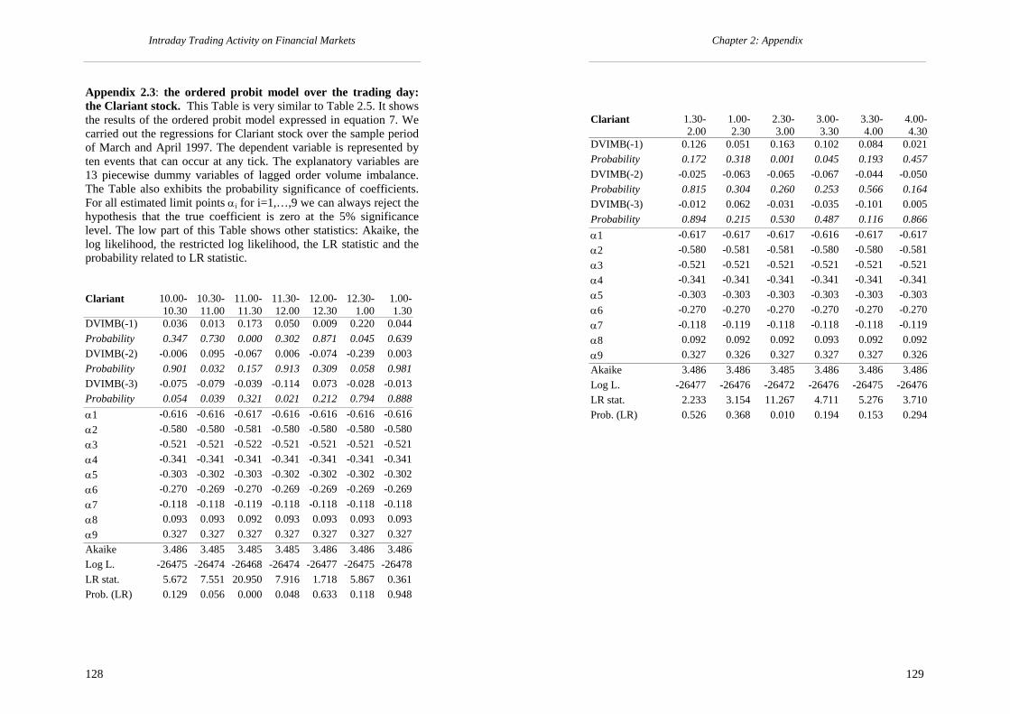
Intraday Trading Activity on Financial Markets
128
Appendix 2.3: the ordered probit model over the trading day: the Clariant stock. This Table is very similar to Table 2.5. It shows the results of the ordered probit model expressed in equation 7. We carried out the regressions for Clariant stock over the sample period of March and April 1997. The dependent variable is represented by ten events that can occur at any tick. The explanatory variables are 13 piecewise dummy variables of lagged order volume imbalance. The Table also exhibits the probability significance of coefficients. For all estimated limit points αi for i=1,…,9 we can always reject the hypothesis that the true coefficient is zero at the 5% significance level. The low part of this Table shows other statistics: Akaike, the log likelihood, the restricted log likelihood, the LR statistic and the probability related to LR statistic. Clariant 10.00-
10.3010.30-11.00
11.00-11.30
11.30-12.00
12.00-12.30
12.30-1.00
1.00-1.30
DVIMB(-1) 0.036 0.013 0.173 0.050 0.009 0.220 0.044Probability 0.347 0.730 0.000 0.302 0.871 0.045 0.639DVIMB(-2) -0.006 0.095 -0.067 0.006 -0.074 -0.239 0.003Probability 0.901 0.032 0.157 0.913 0.309 0.058 0.981DVIMB(-3) -0.075 -0.079 -0.039 -0.114 0.073 -0.028 -0.013Probability 0.054 0.039 0.321 0.021 0.212 0.794 0.888α1 -0.616 -0.616 -0.617 -0.616 -0.616 -0.616 -0.616α2 -0.580 -0.580 -0.581 -0.580 -0.580 -0.580 -0.580α3 -0.521 -0.521 -0.522 -0.521 -0.521 -0.521 -0.521α4 -0.341 -0.341 -0.341 -0.341 -0.341 -0.341 -0.341α5 -0.303 -0.302 -0.303 -0.302 -0.302 -0.302 -0.302α6 -0.270 -0.269 -0.270 -0.269 -0.269 -0.269 -0.269α7 -0.118 -0.118 -0.119 -0.118 -0.118 -0.118 -0.118α8 0.093 0.093 0.092 0.093 0.093 0.093 0.093α9 0.327 0.327 0.327 0.327 0.327 0.327 0.327Akaike 3.486 3.485 3.485 3.485 3.486 3.486 3.486Log L. -26475 -26474 -26468 -26474 -26477 -26475 -26478LR stat. 5.672 7.551 20.950 7.916 1.718 5.867 0.361Prob. (LR) 0.129 0.056 0.000 0.048 0.633 0.118 0.948
Chapter 2: Appendix
129
Clariant 1.30-
2.001.00-2.30
2.30-3.00
3.00-3.30
3.30-4.00
4.00-4.30
DVIMB(-1) 0.126 0.051 0.163 0.102 0.084 0.021 Probability 0.172 0.318 0.001 0.045 0.193 0.457 DVIMB(-2) -0.025 -0.063 -0.065 -0.067 -0.044 -0.050 Probability 0.815 0.304 0.260 0.253 0.566 0.164 DVIMB(-3) -0.012 0.062 -0.031 -0.035 -0.101 0.005 Probability 0.894 0.215 0.530 0.487 0.116 0.866 α1 -0.617 -0.617 -0.617 -0.616 -0.617 -0.617 α2 -0.580 -0.581 -0.581 -0.580 -0.580 -0.581 α3 -0.521 -0.521 -0.521 -0.521 -0.521 -0.521 α4 -0.341 -0.341 -0.341 -0.341 -0.341 -0.341 α5 -0.303 -0.303 -0.303 -0.303 -0.303 -0.303 α6 -0.270 -0.270 -0.270 -0.270 -0.270 -0.270 α7 -0.118 -0.119 -0.118 -0.118 -0.118 -0.119 α8 0.092 0.092 0.092 0.093 0.092 0.092 α9 0.327 0.326 0.327 0.327 0.327 0.326 Akaike 3.486 3.486 3.485 3.486 3.486 3.486 Log L. -26477 -26476 -26472 -26476 -26475 -26476 LR stat. 2.233 3.154 11.267 4.711 5.276 3.710 Prob. (LR) 0.526 0.368 0.010 0.194 0.153 0.294

130
131
CHAPTER 3:
Lead-Lag Relationships between Stocks and
Options

132
Chapter 3: Lead-Lag Relationship between Stocks and Options
133
Abstract
This study investigates the intraday trading patterns and the lead/lag empirical relationships between options and stocks on the Swiss market. While the microstructure literature typically deals with the inter-linkage between trading volume and returns on stock and option markets, we examine lead/lag relationships between option and stock volume, option volume and waiting time to trade stocks and, finally, option volume and stock returns. High frequency data are used to plot the intraday trading patterns while ARCH component and ARCH asymmetric component models are applied to estimate the auto-correlation in market volatility. Our main results indicate that: (1) stock and option intraday patterns exhibit different shapes, (2) trading volumes on the option market lead trading volumes on the stock market, (3) to the same extent, trading volumes on the option market also lead waiting time trading on the stock market, (4) trading volumes on the option market are simultaneously related to stock price changes. The Granger causality test corroborates these causal relationships.

Intraday Trading Activity on Financial Markets
134
3.1. INTRODUCTION
The rationale of this research is that if markets are imperfect and incomplete, then options are not redundant assets. If there are information asymmetry and frictions, then it is possible that the information content of trades is assimilated with different speed by option and stock markets. As observed by Goodhart and O’Hara (1997), unlike studies of individual equity markets, there has been little theory to guide empirical studies of inter-market relationships. Back’s (1993) study is an exception. He provides a model in which trades on the option and on the underlying asset convey different information. In our analysis we also consider trading volumes as a vector of trading information. Consequently, we seek to empirically test (1) if options and stocks markets have a lagged relationship confirming a market imperfection, and (2) if the option market leads the stock market, confirming Black’s (1975) original idea that the higher leverage in option markets induces informed traders to trade in options rather than in stocks.
In so doing, we also study the intraday pattern of option trading volumes. We first compare this pattern with the intraday behavior of stock trading volumes in order to understand their main features. Then we analyze the intraday relationships between option and stock markets. First, we examine the lead/lag relationship between option and stock trading volumes, and observe that stock volumes are driven by option volumes with a slightly large time interval. Second, we carry out a similar analysis of option trading volumes and the waiting time between subsequent trades on the stock market. Here again we observe that option volumes lead trading frequency on the stock market. The relation between option and stock volumes as well as the relation between options volumes and waiting time trading on the stock market presents specific variance equations, namely a persistence pattern modeled through an ARCH process with a transitory and a permanent component. Finally, we examine whether option volumes also lead stock returns and conclude that both react within a period of 15 minutes.
Our study is based on the tick-by-tick data for the most traded stocks on the Swiss Stock Exchange (SWX), during March
Chapter 3: Lead-Lag Relationship between Stocks and Options
135
and April 1997. Since SWX is an electronic order-driven market, this investigation constitutes a new contribution to the understanding of microstructure. Moreover, while inter-market linkages have been studied by an impressive number of researchers, there is very little work that empirically analyses the relationship between option and stock volumes. In particular, no studies deal with the relationship between option volumes and trade frequency on the stock market.
The remainder of this Chapter is organized as follows: in Section 3.2, we provide a detailed review of the previous empirical work in this area. In Section 3.3, we present our data and methodology. In Section 3.4, two topics are discussed: first, the intraday trading volume patterns and, second, the lead/lag relationship between stocks and options markets using high frequency data. Some conclusions and remarks complete Chapter 3. As before, Figures and Tables are presented at the end of the Chapter.

Intraday Trading Activity on Financial Markets
136
3.2. REVIEW OF THE LITERATURE
A. International studies
Patell and Wolfson (1979, 1981) carry out one of the first studies of the relationship between stock and option markets. They analyze the time series behavior of implied variances from options around earnings announcement and show that the time series profile of option prices can predict stock price behavior. As regards earnings announcement, Snelling’s (1987) paper shows that the option market leads the stock market by roughly fifteen minutes during the five trading day period preceding an earnings announcement.
Conrad (1989) and Damodaran and Lim (1991) examine market reactions to the introduction of options rather than announcements. Conrad finds that the introduction of individual options causes a permanent price increase in the underlying security, beginning approximately three days before the option introduction, and that excess return volatility declines accordingly. Damodaran and Lim (1991) study the effects of option listing on returns processes of the underlying securities. The authors also find that (1) the listing of options involves lower variance in the daily returns on the underlying stocks, and (2) there is a speedier price adjustment process to increased information collection after listing.
Manaster and Rendleman (1982) analyze close-to-close returns of portfolios based on the relative difference between real stock prices and theoretical stock prices implied by option prices. They conclude that closing prices of listed call options do, in fact, contain information about equilibrium stock prices that is not contained in the closing prices of the underlying stocks. Furthermore, they claim that it takes up to one day for stock prices to adjust. Thus, the option market appears to lead the stock market. Two explanations are possible for this finding. First, the option market closes ten minutes after the stock market. Therefore, it is possible that the information that Manaster and Rendleman (1982) suppose to be reflected in option prices is only information disseminated between the two closing times. Second, closing option
Chapter 3: Lead-Lag Relationship between Stocks and Options
137
prices may reflect fundamental information about equilibrium values of underlying stocks, which is not contained in closing stock prices.
Bhattacharya’s (1987) paper analyses the intraday lead/lag relation between the option and stock market using bid and ask data on calls to compute implied bid/ask stock prices. These prices are then compared to actual bid/ask stock prices to identify arbitrage opportunity. A stock is considered underpriced (overpriced), if the implied bid (ask) is higher (lower) than the actual ask (bid). A simulated trading strategy based on these arbitrage signals indicates that profits are insufficient to overcome transaction costs for all intraday holding periods. The results indicate that while option prices do seem to contain information not reflected in contemporaneous stock prices, the average difference is insufficient to overcome the bid/ask spread for intraday holding periods. Overnight holding periods result in profits when information search costs and opportunity costs of the exchange seats are not considered. A critical aspect of Bhattacharya’s (1987) study is that it can only detect whether the option market leads the stock market and not vice-versa. Although he shows that option price changes have some predictive power, his results do not preclude the possibility that stock price changes predict option price changes.
Anthony (1988) takes another approach by examining the interrelation between common stock and call option trading volume from January 1, 1982 to June 30, 1983. The study assumes and tests a sequential flow of information between the stock and option market. He concludes that “… trading in call options leads trading in the underlying shares with a one day lag”. These empirical results suggest that option prices contain information not reflected in contemporaneous stock prices, but the evidence is not overwhelming. Moreover, he draws three major conclusions. Among the twenty-five firms investigated, he finds that: (1) option volume leads stock volume for thirteen firms, (2) stock volume leads option volume for four firms, and (3) there is no unambiguous direction of causality for the remaining eight firms. However, his results are subject to the same caveats as Manaster and Rendleman (1982) due to the non-simultaneity of the closing time for the two markets.
Vijh (1988) argues that Manaster and Rendleman’s (1982) methodology suffers from the bid/ask bias as well as non-

Intraday Trading Activity on Financial Markets
138
synchronicity. He concludes that ”not accounting for the bid/ask bounce and the non-synchronicity between stock and option prices, is an ex post study that can give the impression that the option prices lead the stock prices even when the two are in equilibrium”.
Stephan and Whaley (1990) investigate intraday relations between price changes and trading volume of options and stocks for a sample of firms whose options were traded on the CBOE during the first quarter of 1986. The authors circumvent the two major problems diagnosed in the previous studies. First, by using transaction-by-transaction data, they avoid the problem inherent to the non-simultaneity of closing prices in the two markets. Secondly, the analysis focuses directly on the lead/lag relationship between the intraday price changes on the stock and option market rather than indirectly through simulating a trading strategy. Call price changes over five minute intervals are transformed into implied stock price changes, and then multivariate time series regression analysis is used to estimate directly the lead/lag relation between the price changes in the stock and option markets. Unlike the previous studies, their findings indicate that price changes in the stock market lead the option market by as much as fifteen minutes. The analysis of trading volume indicates that the stock market lead may be even longer. In a follow-up study, Chan, Chung and Johnson (1993) come to the same conclusion, finding no evidence that options, even deep out-of-the-money options, lead stocks. Choe, Hyuk, and Freund (1992) find that changing the method of calculating the implied stock price and extending the analysis period do not alter the Stephan and Whaley (1990) results.
The study of Poon (1994) empirically investigates the potential structural shift in the stock return volatility-volume relationship when option trading on the underlying stock is available and tests whether option volume is related to stock return volatility. Two major conclusions emerge. First, there is a structural shift in the relation between stock return volatility and trading volume associated with the introduction of option trading. Second, stock return volatility is found to be significantly and positively related to contemporaneous stock and option volume. These empirical results do not support the contention that, on a daily basis, the option market leads the stock market. However, in the case of some stocks, option
Chapter 3: Lead-Lag Relationship between Stocks and Options
139
listing seems to be a neutral event because neither contemporaneous nor lagged option volume is significant in explaining the conditional variance. In this study the lead/lag relation between stock return volatility and option volume is assumed to be one day. If the lead/lag is less than one day, the structure of the model is not able to test this form of lead/lag linkage.
Nabar and Park (1994) examine empirically whether option trading has an impact on the volatility of underlying stocks. They find evidence of negative excess volatility of underlying stocks after inception of options trading. This contradicts the common belief that option trading increases the volatility of underlying stocks.
Skeikh and Ronn (1994) identify systematic patterns in daily and intraday returns on options detecting whether the option pattern is related to the underlying stock and if so, when. However, their model is based on simultaneous or randomized informed trading on both option and stock markets, so that we cannot apply these findings to lead-lag investigations. Systematic patterns in intraday trading volume and spread are also analyzed by Chan, Chung and Johnson (1995). In particular, they study the intraday behavior of bid-ask spreads for actively traded CBOE options and for their NYSE-traded underlying stocks. They find divergent intraday patterns on option and stock markets. In order to explain this difference, the authors evoke the differences between CBOE and NYSE market structure.
Mayhew, Sarin and Shastri (1995) approach the analysis of the option and stock market inter-linkage from another point of view. They examine the impact of margin changes in the options market and its underlying stock. The authors find that a margin decrease is associated with increases in bid-ask spreads and in the information content of stock trades, but also with decreases in the underlying stock market depth and in spreads in the options market. For our proposes, the most important conclusion is that a decrease in the margin component of trading costs seem to cause migrations of uninformed traders from the stock to the option market, and vice versa.
Diltz and Suhkyong’s (1996) study reconciles conflicting results by Manaster and Rendleman (1982) and Stephan and Whaley (1990) regarding the price change relationship between options and

Intraday Trading Activity on Financial Markets
140
their underlying stocks using a methodology designed to circumvent the non-synchronicity and the bid/ask bias problem that may have affected earlier studies. The analysis covers eight firms whose options and stocks are actively traded on CBOE and NYSE, respectively. Only call options are included in the analysis. With this adjustment, their empirical results are consistent with those of Manaster and Rendleman (1982), indicating that option price changes lead stock price changes over two trading days.
The study by Assogbavi, Khoury and Yourougou (1995) adds a significant contribution in this regard as it investigates the Toronto Stock Exchange and provides empirical evidence to the asymmetry in the price-volume relationship.
The final international study presented here was carried out by Easely, O’Hara and Srinivas (1998) who investigated the informational role of transaction volume in option markets. Their intuition is that if the option market is more attractive to informed traders, then option trades may primarily reflect information content. Their principal empirical finding is that news on option volumes has a predictive power for stock price movements.
B. Swiss Studies
Three studies look at the interaction between the markets. The first study was carried out by Pirotte and Tamburini (1994). They investigated the lead/lag relationship between the SMI futures and the underlying Index. Using daily closing prices from 1990 to 1994 and different testing procedures, mainly the Granger causality test and VAR (vector auto-regression model), they conclude that the Index leads the futures market. This result may be due to the non-synchronicity of their closing prices since the SOFFEX closes five to ten minutes after the Stock Exchange and may thereby exhibit inertia in its price setting mechanism around closing time. It is also more difficult to believe that the market Index and not a specific asset involves an asymmetry of information, therefore it is more unlikely that options lead the underlying stock market Index.
Stucki and Wasserfallen (1994) analyze the lead/lag relationship between individual stock prices and their corresponding
Chapter 3: Lead-Lag Relationship between Stocks and Options
141
call prices using intraday data and the same methodology as Stephan and Whaley (1990). The results suggest that price changes on the stock market lead price changes on the option market for actively traded call options. On average lead-time is about ten minutes. To summarize, the Swiss evidence confirms the results obtained by Stephan and Whaley (1990) for the US market.
The last study was done by Bruand and Gibson-Asner (1995). They also use intraday data to examine the price dominance relationship between the various cash and derivatives market segments. They extend the analysis in several directions applying a different methodology than Stucki and Wasserfallen (1994). In order to test for leads and lags in the prices quoted on different market segments, Bruand and Gibson-Asner analyze one month at-the-money American calls written on Ciba-Geigy, Nestlé, Roche and UBS, that is a sample of the most actively traded Swiss stocks. In contrast to the results reported by Stucki and Wasserfallen (1994) for individual stock options during 1989, they find that there is no significant lead or lag between Nestlé stock and option price series, a weak dominance of the Ciba-Geigy call price which disappeared over time, and that UBS and Roche calls lead their underlying stock market prices by twenty minutes on average.

Intraday Trading Activity on Financial Markets
142
3.3. DATASET, MARKET STRUCTURE AND METHODOLOGY
A. Dataset and Market Structure
In this Chapter we examine the intraday trading relationship between listed call and put options and their underlying common shares during the month of March 1997 in the Swiss market. Most specifically, we analyze: (1) intraday patterns on option and stock markets, (2) the relationship between intraday trading volumes of options and their underlying assets, (3) the relationship between intraday trading volumes of options and waiting time between subsequent trades of the underlying asset, and (4) the relationship between intraday trading volume of options and the underlying asset’s returns.
We have chosen to study the Novartis1 stock since it is the most liquid asset on the Swiss stock market according to several market liquidity proxies (see Chapter 1). Trading activity on Novartis stocks began in the year 1996 while trading on options started on February 26, 1997. Apart from being listed on the Swiss market (Swiss Stock Exchange and SOFFEX), Novartis is also listed outside Switzerland, in London (N; Seaq) and USA-OTC (ADR N). We are aware that multiple listings may generate some bias. Yet it is important to emphasize that most trades, in number and volume, take place on the Swiss Stock Exchange. Furthermore, we must take into consideration the role of asymmetric information and of discretionary liquidity traders. More specifically, we have to recognize that (1) when a stock is quoted on several markets, stock liquidity on each market decreases because the total order flow is divided between markets, as shown by Mendelson (1987), and then (2) traders concentrate their activity on some specific markets (Pagano 1989 a, b) and during some specific sub-periods (Admati and Pfleiderer, 1988; Foster and Viswanathan, 1990 and 1993). Hence, the geographical and temporal aggregation of the intraday
1 From the merger between Ciba-Geigy and Sandoz in 1996. Novartis is now the second largest pharmaceutical firm in the world with a market share of 4.5%. The Reuter Ric is NOVZn.S
Chapter 3: Lead-Lag Relationship between Stocks and Options
143
trading activity on the Swiss market renders other markets of secondary importance.
As far as the market structure is concerned, the Swiss market has changed, in the nineties. Before 1990, we had a number of different stock exchanges (e.g. Zurich, Geneva, Basel, Bern, Lausanne, Neuchâtel and St. Gallen), and in addition we had the Swiss Options and Financial Futures Exchange (SOFFEX), which started trading on May 19, 1988. In 1991, a certain number of stock exchanges closed, and one year later a computerized trading system project was put in place. Starting on August 2,1996 the Swiss Stock Exchange became a fully computerized trading system where the matching of orders occurs automatically. Seven regional stock exchanges and the SOFFEX were subsumed into one organization with a computerized system (SWX 1996 a, b). The Swiss market is an order-driven-market with a limit order book, similar to the Paris Bourse or the Toronto Stock Exchange. In an order-driven market, orders are submitted and then trading prices determined. An order-driven system can be a continuous auction in which traders submit orders for immediate execution against an existing limit order or it can be structured as a call market or batch trading system in which orders accumulate and are cleared at period intervals (O’Hara, 1995). The Swiss stock exchange is a continuous market in which the computer stores all orders in a public limit order book. The limit-order book is the hub of these automated systems. When viewing all standing orders, a trader knows exactly what trades will be executed if he or she enters a new quota or limit order. The structural difference between the SWX and the SOFFEX is that the latter is a price driven market, that is, an exchange system where the traders must trade with a market-maker who continuously provides a bid and an ask quotes (SOFFEX 1992).
The data tested in this empirical study come from three sources2. First, the SOFFEX provided option (call and put) high frequency transaction data during March 1997. These data contain the time, the expiry year, the expiry month, the exercise price and the number of contracts traded for each option transaction. Second, the
2 This data set was graciously provided by the Swiss Stock Exchange in Zurich.

Intraday Trading Activity on Financial Markets
144
number of option contracts still open was collected daily from the AGEFI during the estimation period. Third, a SWX data set was used to collect intraday stock transaction data.
B. Methodology
This study has three main objectives. First, we want to verify the existence of an intraday liquidity pattern of options trades by detecting its main features. Second, we want to investigate the intraday relationship between options and their underlying stocks with respect to trading volumes, and waiting time between trades and returns. Third, using the Granger causality test, we want to find whether there is a significant causal relationship between volumes on the two markets. The chosen methodology is discussed below.
As a first step, in order to organize the data, a time series of trading volume, waiting time trading on stock market and return on stocks must be defined over time intervals of a fixed length. We have decomposed the trading day into twenty-six intervals of fifteen minutes each. To circumvent the problem of the non-synchronicity of the closing time of the two markets, we have decided to increase the last interval of the options to twenty minutes instead of fifteen. We take into consideration six standardized time series: cumulated trading volumes on stock market, labeled SVOL, cumulated volumes of call and put options (VCP), cumulated volumes of call options, labeled VCALL, cumulated volumes of put options (VPUT), the mean on each period of 15 minutes of the waited time between subsequent trades on stock market (SWAIT), and, finally, returns on stock market (SRETURN). More precisely, trading volume on stocks for the period i, SVOLi, is calculated in the following way:
m.f
vSVOL
n
1ti,t
i
∑==
SVOLi indicates the cumulated trading volumes on stocks during the period of 15 minutes i, where i=1, …, 26. Transaction volume is vt, trade time during each period of 15 minutes is indexed with t=1,…,n, while the total number of shares outstanding is a
Chapter 3: Lead-Lag Relationship between Stocks and Options
145
constant m, and f is another constant indicating the percentage of free float.
The procedure for calculating the ratio of trading volume on the option market relates trading volumes during each period of 15 minutes, i, to the number of contracts still open at the end of the trading day, j. Then, we add up the resulting ratios for each type of option according to different exercise prices, expiry month and expiry date. That is:
v
vVPUT ,
v
vVCALL
pl
pj,t
n
1t
pj,i,t
j,ip
l
cj,t
n
1t
cj,i,t
j,i ∑ ∑∑
∑ ∑∑
== ==
ji,ji,ji, VPUT VCALLVCP +=
where VCALLi,j (VPUTi,j) indicates the ratio of the cumulated trading volumes on calls (puts) during the period of 15 minutes i, where i=1, …, 26, for the day j.. Transaction volume traded on call (put) option is vc
t (vpt), trade time during each period
of 15 minutes is indexed with t=1,…,n, the total number of open contracts is indexed with l=1, …, L, and all types of options are indexed with p= 1, …,P. As far as waiting time between subsequent trades is concerned, we calculate its mean over each period of 15 minutes:
( )∑=
+ −=n
1ti,ti,1ti trtr
n1WAITS
where SWAITi is the acronym indicating the mean waiting time between subsequent trades over the period of 15 minutes i, where i=1, …, 26, and trt,i indicates trade time within the 15 minutes i, with t=1,…,n,. Returns are estimated as usual (named continuously compounded return, as in Campbell, Lo and MacKinlay 1997):
( ) ( )i,1i,ni plnplnRETURN −=
We calculate the return over the period of 15 minutes i by considering the logarithmic difference between the initial and the final price.

Intraday Trading Activity on Financial Markets
146
Each variable was standardized, i.e. from each value referring to a period of 15 minutes we subtracted its daily mean and then this difference was divided by the daily standard deviation. For each time series we carried out the unit root test, namely the augmented Dickey-Fuller tests finding that all the time series are largely above the MacKinnon critical values for the rejection of the hypothesis of a unit root. We also verified the features of the distribution for each time series through the Jarque-Bera test indicating normal distributions with mean zero and standard deviations one.
Chapter 3: Lead-Lag Relationship between Stocks and Options
147
3.4. EMPIRICAL FINDINGS
The intraday trading volume patterns are examined with the help of Figure 3.1. In the graph the simple line represents the standardized trading volume of the stock in each fifteen minute interval of the working day, the line marked with a square represents standardized trading volume of the call, and, finally, the line marked with a circle represents the standardized trading volume of the put.
As observed in Chapter I, trading volumes on a stock market may be considered a liquidity proxy indicating that Swiss intraday liquidity patterns do not precisely follow a U-shape (as, among others, in Jain and Joh 1988, McInish and Wood 1990) nor an M-shape (as in Gouriéroux, Jasiak and Le Fol., 1997). The Swiss stock exchange seems to follow a triple U-shaped pattern3.
In comparison with stock volumes, we notice interesting differences in the intraday behavior of option patterns. First, the intensity of put and call option trading activity reaches a peak about one hour after the opening. This result is consistent with the empirical findings in Chan, Chung and Johnson (1995) and Easley, O’Hara and Srinivas (1998) who observe that option patterns present the maximum level of liquidity about 45 minutes after the open time. Second, option patterns have several sharp rises even during the lunch period while the lunch time on the stock market is characterized by persistent illiquidity trading. We can explain this difference considering again the role of a discretionary liquidity trader and an informed trader. Discretionary liquidity traders find a pooling equilibrium on the stock market during high liquidity periods and not during low volume times such as the lunch period. Furthermore, these moments of high market liquidity allow informed traders to hide their informed transactions, thus further increasing liquidity. In contrast, the randomized arrival of insider information and the prevalent presence of informed traders on the option market generates a more irregular intraday trading pattern on options. Thirdly, afternoon peaks are not as high as morning ones, especially for calls. This is also analogous to the empirical findings in Chan,
3 For a more detailed describtion see Chapter 1, Section 1.3.

Intraday Trading Activity on Financial Markets
148
Chung and Johnson (1995) and in Easley, O’Hara and Srinivas (1998).
However, intraday trading patterns of options, like patterns on stocks, follow the usual U-shape at least at the end of the trading day (as in, e.g., Stephan and Whaley 1990). We finally notice that while trading activity on stocks and call on Swiss markets is suspended before US markets open, trading activity on put does not stop. This confirms the essential dependence of Swiss markets upon US markets and it may suggest that put are used as hedging tools.
In the light of existing differences between intraday trading patterns on stock and option markets, it would be interesting to test by regression whether a linkage between the two markets exists. To conduct this test we have considered the overall sample, that is, four hundred and sixty-eight observations, using the following model:
(1) VCPVSTOCKVSTOCK tk
ktk1tt ε+β+α= ∑ −−
After performing ARCH regression analysis, Table 3.1 exhibits the significant results with respect to option (call and put volumes summed up) and stock volumes.
We observe that trading volumes on stock present an AR(1) and a significant relation with contemporaneous and lagged options volumes. We find that the relations between stock and option volumes reach 3 lags, i.e. around 45 minutes, with positive and decreasing coefficients. Moreover, the results from the variance equation in Table 3.1 indicate significant decomposition of conditional variance into a permanent component and a transitory component combined with a TARCH model to allow asymmetry. Therefore we structure conditional variance as:
( ) ( )( ) ( ) ( ) (3) qdqqq
(2) cqcq
1t2
1t1t1t2
1t1t2
1tt2t
21t
21t1tt
−−−−−−−
−−−
−σβ+−εγ+−εα+=σ
σ−εφ+−ρ+=
In equation (3) σ2t indicates current volatility and in
equation (2) qt refers to long run volatility. In equation (2) c,ρ andφ indicate the constant long run volatility and two coefficients,
Chapter 3: Lead-Lag Relationship between Stocks and Options
149
respectively. In equation (3) α,γ and β are the coefficients of the current volatility equation and dt-1 is the dummy variable that allows us to recognize whether an asymmetric effect on the conditional variance exists. While (σt–qt), i.e. the difference between current and long run volatility, converges to zero with powers of (α+γd+β), qt, i.e. the permanent component, converges to zero with powers of (ρ). Given that ρ is not so far from 1, we observe that the long run volatility approaches the constant, c, rather slowly. We also notice that the coefficient of lagged long run volatility, (q-c), is near 1 while the coefficient of the difference between ARCH and GARCH component nears zero. This signals that the lagged value of long run volatility strongly determines its permanent value. Furthermore, we point out that current volatility, σ2
t, is largely defined by its permanent value, q, since two of three transitory components, i.e. (ARCH-q) and (GARCH-q), are not significantly different from zero. However, we notice that the ARCH component, i.e. (ARCH-q), acquires importance for negative residuals that reduce current volatility and generate an asymmetric effect. Interpreting residuals of trading volume as news arrival (Lamoureux and Lastrapes (1990)), negative shocks slightly decrease market activity reducing intraday market depth. Moreover, similarly as the Hasbrouck’s argument (1991), the presence of temporary and permanent volatility suggests that we can recognize two kinds of information impact. The former has a short run consequence represented by the temporary changes in trading activity. This is typically generated by the arrival of public information. The more efficient the market is, the faster the market absorbs the impact of public information. The latter involves a longer market impact and can be produced by the trading activity carried out by informed traders. Informed traders have an interest in disguising their identity and information, and private information disclosure is therefore gradual and slow.
Table 3.2 reports empirical findings resulting from the regression of call and put volumes options on stock trading volumes on the stock market, equation (4) and (5), respectively.

Intraday Trading Activity on Financial Markets
150
(5) VPUTLVSTOCKVSTOCK
(4) VCALLVSTOCKVSTOCK
tk
ktk1tt
tk
ktk1tt
ε+β+α=
ε+β+α=
∑∑
−−
−−
We observe similar features and coefficients for calls and puts, even if we consider that (1) for call options the twice-lagged variable is less significant, and (2) all variance components of call options present significant coefficients whereas the permanent component provided by the difference between the ARCH and the GARCH components and the asymmetric ARCH component for the put option are not significantly different from zero.
Furthermore, we also notice that variance equations for puts and calls present the same coefficients in absolute value, but consistently with opposite sign since options reaction to news arrival is opposite depending on the type of option, i.e. if a call or a put is traded. One of the most important coefficients is the GARCH transitory component of the conditional variance, or (GARCH-q), for both call and put, but with opposite signs.
This means that a relatively high current volatility implies a relatively high volatility in the following periods for call options, and vice versa for put options. Linking volume volatility and news arrivals suggests that call options are the main vector of information disclosure whereas the put options are probably less frequently traded since they are mainly used as hedging instrument. This is also confirmed by both permanent components, (q-c) and (ARCH-GARCH), presenting opposite signs. We finally notice that the asymmetric component, (ARCH-q)d, is significant and negative only for the call option. This result indicates that bad news fundamentally reduces temporary market activity but, at same time, the asymmetric component is not significant for the put option suggesting again its refractory behavior in terms of temporary trading activity and reinforcing the idea of a prevalent hedging use.
Table 3.3 clearly indicates that trading volumes on options and waiting time to trade on stocks have a negative relationship, as follows:
Chapter 3: Lead-Lag Relationship between Stocks and Options
151
A negative relationship was also found between waiting
time and trading volumes on the Swiss stock exchange (see Chapter 1). Both provide a market liquidity proxy, but trading volume more appropriately refers to market depth and waiting time trading to the time domain of market liquidity. This means that an increase in option volumes implies a wider information disclosure involving a rise in trading activity in terms of transaction frequency.
However, our results show that current and lagged trading volumes on options up to about 45 minutes contribute to explaining this relationship. As for the previous results (Tables 3.1 and 3.2), the more recent the coefficient, the bigger its value. Again, the variance equation can be decomposed into a constant, two asymmetric ARCH components and a GARCH component, but not into a permanent and transitory variance.
Hence, equation (3) becomes:
(7) d 21t1t
21t
21t
2t −−−− βσ+γε+αε+ω=σ
The main difference is that the long run volatility in equation (3), qt, becomes a constant, ω. The lagged GARCH component together with the constant constitutes the main explanation variables of the variance equation. We notice that good news does not significantly affect volatility of trade frequency on stocks through the positive ARCH component, here ARCH(1), while the opposite is true for bad shocks, here (d<0)ARCH(1). This indicates that negative news slows up trading activity, not only by reducing liquidity depth, as we have seen before for the call option, but also by decreasing trade frequency.
In Table 3.4 we analyze the relation between the waiting time trading on the stock market and volumes of calls and puts, separately as follows:
(6) VCPSWAITSWAIT tk
ktk1tt ε+β+α= ∑ −−
(9) VPUTSWAITSWAIT
(8) VCALLSWAITSWAIT
tk
ktk1tt
tk
ktk1tt
ε+β+α=
ε+β+α=
∑∑
−−
−−

Intraday Trading Activity on Financial Markets
152
In view of the results in Table 3.4, the current and the first lagged coefficients of call option volumes are more closely linked to waiting time trading on stock market. Coefficients are negative for calls and puts reflecting the fact that volumes are linked to information which brings about stock transactions.
The variance equations for calls and puts present similar features. However, we observe that the asymmetric component for put options was not significantly different from zero when we regressed option volume on stock volume (see Table 3.2) but it did when we regressed put option volume on waiting time trading on the stock market (Table 3.4). This means that when bad news arrives the put market reacts reducing intraday market liquidity in terms of trade frequency but not in terms of depth. As in Chapter 1, we find that the time dimension of intraday market liquidity has an informational content. This factor shows that trade frequency is influenced by both informational and strategic considerations.
The last investigation takes into consideration stock returns and option volumes (Table 3.5) as follows:
(11) VPUTVCALLRETURNRETURN(10) VCPRETURNRETURN
ttt1tt
tt1tt
ε+η+β+α=ε+β+α=
−
−
Our tests indicate that these two elements are simultaneously related: no lagged option volume has a significant contribution in this relation. This is consistent with Easley, O’Hara and Srinivas (1998) who find, among other things, no evidence that put or call option volumes lead stock price changes. We also find that the simultaneous relationship between option volume and stock return is positive, and that a rise in option trading volume implies a rise in stock return.
Separating call and put option volume (as in Table 3.5.B), we notice that call volume has a weak relationship to stock returns. This may be due to the fact that the underlying stock shows close-to-close negative returns during more than half of our estimation period. As to the variance equation, we observe that (1) the coefficient of the constant, c, is relatively high, (2) the other two
Chapter 3: Lead-Lag Relationship between Stocks and Options
153
coefficients of the permanent components, (q-c) and (ARCH-GARCH), are also significant and positive, and (3) the asymmetric ARCH components, (ARCH-q) and (ARCH-q)d, are negative, so that both positive and negative shocks are negatively related to current volatility, but with different response parameters.
If we compare the results in Table 3.1, 3.2 and 3.3, we see that the power of convergence of (σt–qt), i.e. the difference between current and long run volatility, to zero corresponds to (α+γd+β), and it is larger in absolute value when we regress the option volume on stock returns than when we regress the option volume on stock volume. In the former case, this means that the current volatility moves quickly away from the long run volatility. Considering the power of convergence of qt, i.e. the permanent component, to zero, we notice that the regression of option volume on stock returns presents a smaller coefficient, ρ, in absolute value. Consequently, the long run volatility, qt, approaches the constant, c, more slowly than in the regression in which stock volume is the dependent variable. This predominance of current volatility in the variance equation of volume/returns regression suggests a faster adjustment of stock returns to option volume dynamics and therefore justifies the simultaneous relationship between these variables and the absence of lagged explanatory variables in Table 3.5.
Using the Granger causality test, we now investigate whether trading activity on option and stock markets is causally related in the Granger sense. The test methodology was applied twice: first, we test whether it is true that the volume of trading in the option market does not cause trading volume, return and trading time in the stock market, we then test the opposite. In each case, the regressions were run with three lags.
The results are summarized in Table 3.6. They indicate that we cannot accept the hypothesis that (1) option volumes do not Granger cause stock volumes, (2) call option volumes do not Granger cause stock volumes, (3) put option volumes do not Granger cause stock volumes, and, (4) put option volumes do not Granger cause trade frequency on stock market. Our results also suggest that we can accept the hypothesis that (1) stock volumes do not Granger cause options volumes (put and call added up, and put singularly), (2) waiting time trading on stock market does not Granger cause put

Intraday Trading Activity on Financial Markets
154
options volumes, (3) stock returns do not Granger cause options volumes (put and call added up, and put singularly). All these empirical findings support our previous results indicating that option leads stock. The only unsatisfactory result concerns the Granger causality between option volumes and waiting time trading on the stock market. Even if we find that put volume causes stock trade frequency, we would expect the same result for calls, and for calls and puts volumes together.
Chapter 3: Lead-Lag Relationship between Stocks and Options
155
3.5. CONCLUSIONS
The purpose of this Chapter is to investigate (1) whether some intraday trading patterns on option and stock on the Swiss markets exist, and (2) whether option and stock markets do have a lagged relationship confirming market inefficiency. Our analysis was carried out on tick-by-tick data.
The first part of this study describes intraday trading patterns on the SOFFEX option market and on the Swiss stock market. Two major conclusions emerge. First, we find that Swiss stocks and Swiss options have characteristic intraday patterns, a sort of mix of the M-shape and the usual U-shape known in the literature. Second, intraday option patterns do not imitate intraday stock patterns and, moreover, intraday liquidity behavior of call options is also distinct from the put pattern, confirming previous findings (e.g., Chan, Chung and Johnson 1995 and Easley, O’Hara and Srinivas 1998).
The second objective of this study, i.e. to discover whether option and stock markets do have a lagged relationship, sheds some new light on the microstructure literature dealing with inter-market linkages. While these studies typically focus on the interaction between trading volume and returns on stock and option markets, our contribution also analyzes the lead/lag relationships between option and stock volume, option volume and stock waiting time trading. The results show that (1) standardized trading volume on the option market leads standardized stock trading volumes, and the lead time is around 45 minutes (2) in a similar way, option volume also leads standardized waiting time trading on stock market, and (3) option volume and stock returns have a simultaneous relationship. Hence, on the one hand our results bear out the absence of a lagged volume/return relationship linking option and stock markets, and, on the other hand, they provide new arguments supporting the idea that trading activity on options leads trades on stocks.
After data transformation, we performed regressions based on the ARCH component model regression, on the ARCH asymmetric component model and, finally, on the TARCH model. Appropriately recognizing the asymmetric and transitory

Intraday Trading Activity on Financial Markets
156
components involved in the variance equations, we provide new explanations of the different market reactions to news arrivals distinguishing between public and private information disclosures, and between bad and good news. The diffusion of public news seems to support a temporary volatility in terms of intraday market activity while the disclosure of private information involves a gradual and persistent impact. Furthermore bad news decreases intraday market liquidity reducing both liquidity depth and trade frequency. These results become even more intriguing if we consider put and call options separately. The empirical findings indicate that call and put options are used in a different manner and with dissimilar purposes. The former functions as a wider and more speculative trading instrument whereas the latter is mainly used as a hedging instrument.
We finally examine the Granger causality between all the variables and find new evidence of previous results on the lead/lag relationships, i.e. option volume leads stock volume and transaction frequency on the stock market, and not the other way around.
Chapter 3: Figures
157
3.6. FIGURES
Figure 3.1: Intraday trading patterns. Figure 3.1 shows the intraday trading patterns on the Swiss stock and option markets of the Novartis stock, call and put options, over the period of March 1997. The trading day is decomposed in to 26 intraday periods of 15 minutes (horizontal axis). Each time series of trading volume has been subtracted by its mean and then divided by its standard deviation in order to obtain a standardized measure of trading volume (vertical axis).
-1.5
-1
-0.5
0
0.5
1
1.5
2
1 3 5 7 9 11 13 15 17 19 21 23 25
Intraday Periods of 15 min.
Stan
dard
ized
Tra
ding
Vol
ume
CallPutStock

158
Chapter 3: Tables
159
3.7. TABLES Table 3.1: Intraday relationships between stocks and options. To perform this regression, we used the transaction data of the Novartis stock over the sample period of March 1997. Table 3.1 shows the results of an ARCH regression represented by equation (1) in which standardized trading volumes on stocks, VSTOCK, is the dependent variable while the explanatory variables are an AR(1) of stock volumes and standardized lagged trading volumes on options, VCPt-k (volumes of call and put summed up). The regression is based on a (adjusted) sample 468 observations and convergence was achieved after 125 iterations. The conditional variance equation is based on a component ARCH model including asymmetric, transitory and permanent components (see equation 2 and 3).
Table 3.1 Variable Coeff. Std. Error t-Stat. Prob. VCP 0.215 0.021 10.065 0.000 VCP(-1) 0.094 0.026 3.651 0.000 VCP(-2) 0.043 0.027 1.591 0.112 VCP(-3) 0.055 0.027 2.049 0.041 AR(1) 0.345 0.039 8.845 0.000
Variance Equation c 0.722 0.045 15.974 0.000 (q-c) 0.968 0.007 136.44 0.000 (Arch-Garch) -0.046 0.000 -11775 0.000 (Arch-q) 0.022 0.037 0.596 0.552 (Arch-q)d -0.017 0.006 -2.708 0.007 (Garch-q) 0.610 0.874 0.698 0.485 R-squared 0.295 Mean dependent var -0.004 A. R-sq. 0.279 S.D. dependent var 0.982 S.E. of regr. 0.833 Akaike info criterion -0.341 SSR 314.6 Schwarz criterion -0.243 Log likel. -557.2 F-statistic 30.799 D-W stat. 2.071 Prob(F-statistic) 0.000

Intraday Trading Activity on Financial Markets
160
Table 3.2: Intraday relationships between call, put and stock volumes. Table 3.2.A shows the results of an ARCH regression represented by equation (4) in which standardized trading volumes on stocks, VSTOCKt, is the dependent variable while the explanatory variables are an AR(1) of stock volumes and standardized lagged trading volumes on call options, VCALLt-k. Table 3.2.B shows the same ARCH regression when trading volumes on put options VPUTt-k represent the explanatory variables, see equation (5). Regressions are based on a (adjusted) sample of 468 observations and convergence was achieved after 125 and 22 iterations for call and put, respectively. The conditional variance equation is based on a component ARCH model including asymmetric, transitory and permanent components (see equation 2 and 3). To perform this regression, we used the transaction data of the Novartis stock over the period of March 1997.
Table 3.2.A Table 3.2.BVariables Coeff. t-Stat. Prob. Variables Coeff. t-Stat. Prob.VCALL 0.227 6.099 0.000 VPUT 0.307 11.201 0.000VCALL(-1) 0.146 3.833 0.000 VPUT(-1) 0.151 3.992 0.000VCALL(-2) 0.069 1.627 0.105 VPUT(-2) 0.084 2.197 0.029VCALL(-3) 0.124 3.274 0.001 VPUT(-3) 0.073 2.150 0.032AR(1) 0.372 9.333 0.000 AR(1) 0.352 9.760 0.000Variance Variance c 0.770 28.471 0.000 c 0.692 10.764 0.000(q-c) 0.979 158.0 0.000 (q-c) -0.963 -45.47 0.000(Arch-Garch) -0.017 -6.960 0.000 (Arch-
Garch) 0.029 1.580 0.115
(Arch-q) -0.028 -1.906 0.057 (Arch-q) -0.072 -3.019 0.003(Arch-q)d -0.006 -3.030 0.003 (Arch-q)d 0.066 1.144 0.253(Garch-q) 0.972 28.674 0.000 (Garch-q) -0.609 -3.259 0.001A. R-sq. 0.221 Akaike -0.263 A. R-sq. 0.258 Akaike -0.312Log likel. -575.8 F-stat. 14.143 Log likel. -573.0 F-stat. 17.097D-W stat 2.105 Pr(F) 0.000 D-W stat 2.120 Pr(F) 0.000
Chapter 3: Tables
161
Table 3.3: Intraday relationships between option volumes and the waiting time to trade on the stock market. Table 3.3 shows the results of the ARCH regression shown in equation (6) in which standardized waiting time between subsequent trades on stocks markets, SWAITt, is the dependent variable while the independent variables are an AR(1) of waiting time and standardized lagged trading volumes on options, VCPt-k (volumes of call and put added up). The regression is based on an (adjusted) sample of 468 observations and convergence was achieved after 9 iterations. The conditional variance equation is based on a TARCH model including a dummy variable related to the negative ARCH component. To perform this regression, we used the transaction data of the Novartis stock over the period of March 1997.
Table 3.3 Variable Coefficient Std. Error t-Statistic Prob. VCP -0.173 0.039 -4.429 0.000 VCP(-1) -0.153 0.048 -3.181 0.002 VCP(-2) -0.122 0.051 -2.408 0.016 VCP(-3) -0.096 0.042 -2.294 0.022 AR(1) 0.400 0.032 12.615 0.000
Variance Equation C 0.352 0.122 2.885 0.004 Arch(1) 0.014 0.049 0.283 0.777 (d<0)Arch(1) -0.335 0.136 -2.471 0.014 Garch(1) 0.670 0.059 11.305 0.000 R-squared 0.351 Mean dependent var 0.005 A. R-sq. 0.340 S.D. dependent var 0.984 S.E. of regr. 0.800 Akaike info criterion -0.428 SSR 290.9 Schwarz criterion -0.348 Log likel. -565.4 F-statistic 30.799 D-W stat. 1.887 Prob(F-statistic) 0.000

Intraday Trading Activity on Financial Markets
162
Table 3.4: Intraday relationships between call and put volumes, and the waiting time to trade on the stock market. Table 3.4.A shows the results of a TARCH regression expressed in equation (10) in which standardized waiting time between subsequent trades on stocks markets, SWAITt, is the dependent variable while the independent variables are an AR(1) of waiting time and standardized lagged trading volumes on call options, VCALLt-k. Table 3.4.B shows the same TARCH regression based on equation (11) when trading volumes on put options represent the explanatory variables, VPUTt-k. Regressions are based on an (adjusted) sample of 468 observations and convergence was achieved after 6 and 8 iterations for calls and puts, respectively. The conditional variance equation includes a dummy variable related to the negative ARCH component (see equation 7). To perform this regression, we used the transaction data of the Novartis stock over the period of March 1997.
Table 3.4.A Table 3.4.BVariable Coeff. t-Stat. Prob. Variable Coeff. t-Stat. Prob. VCALL -0.227 -4.403 0.000 VPUT -0.209 -5.020 0.000VCALL(-1) -0.250 -8.932 0.000 VPUT(-1) -0.188 -2.855 0.005VCALL(-2) -0.125 -2.508 0.013 VPUT(-2) -0.219 -3.037 0.003VCALL(-3) -0.145 -2.910 0.004 VPUT(-3) -0.129 -1.837 0.067AR(1) 0.454 13.904 0.000 AR(1) 0.433 30.081 0.000Variance Variance C 0.160 3.348 0.001 C 0.166 3.594 0.000Arch(1) 0.001 0.054 0.957 Arch(1) 0.007 0.279 0.780(d<0)Ar(1) -0.316 -6.502 0.000 (d<0)Ar(1) -0.328 -4.665 0.000Garch(1) 0.877 51.672 0.000 Garch(1) 0.855 36.078 0.000A. R-sq. 0.333 Akaike -0.417 A. R-sq. 0.327 Akaike -0.409
Log likel. -574.1 F-stat. 29.840 Log likel. -555.0F-statistic
29.157
D-W stat 1.959 Pr(F) 0.000 D-W stat 1.915 Prob(F-s.) 0.000
Chapter 3: Tables
163
Table 3.5: Intraday relationships between option volumes and stock returns. Table 3.5.A shows the results of an ARCH regression expressed in equation (10) in which standardized returns in absolute value on stocks markets, RETURNt, is the dependent variable while the explanatory variables are AR(1) of return and standardized trading volumes on options (volumes of call and put added up), VCPt. Table 3.5.B refers to equation (11). Dependent variables in Table 3.5.B distinguish volumes of call and put, VCALLt and VPUTt. We verified the absence of multicollinearity. The regression is based on an (adjusted) sample of 468 observations and convergence was achieved after 42 iterations. The conditional variance equation is based on an asymmetric ARCH component model including a dummy variable related to the negative ARCH component (see equation 2 and 3). To perform this regression, we used the transaction data of the Novartis stock over the period of March 1997.
Table 3.5.A Table 3.5.B
Variable Coeff. t-Stat. Prob. Variable Coeff. t-Stat. Prob. VCP 0.091 3.921 0.000 VCALL 0.059 1.613 0.108 AR(1) 0.163 3.284 0.001 VPUT 0.135 3.281 0.001
AR(1) 0.163 3.437 0.001 Variance Variance c 1.014 12.566 0.000 c 0.984 13.302 0.000 (q-c) 0.483 6.476 0.000 (q-c) 0.494 4.022 0.000 (Arch-Garch)
0.367 3.064 0.002 (Arch-Garch)
0.332 1.941 0.053
(Arch-q) -0.333 -3.116 0.002 (Arch-q) -0.313 -1.933 0.054 (Arch-q)d -0.239 -3.618 0.000 (Arch-q)d -0.217 -3.198 0.002 (Garch-q) 0.364 1.228 0.220 (Garch-q) 0.338 0.885 0.377 A. R-sq. 0.029 Akaike -0.049 A. R-sq. 0.030 Akaike -0.049 Log likel. -630.9 F-stat. 3.004 Log likel. -630.4 F-stat. 2.831 D-W stat 2.060 Pr(F) 0.004 D-W stat 2.062 Pr(F) 0.004

Intraday Trading Activity on Financial Markets
164
Table 3.6: Granger causality test results. This Table shows the results of the Granger causality test among intraday market variables, namely volume of call and put options added up (VCP), call volume (VCALL), put volume (VPUT), stock volume (VSTOCK), the mean of the waiting time between subsequent trades on stock market (SWAIT) and stock return (RETURN). All these variables are standardized and calculated over intraday periods of 15 minutes. To perform this test, we used the transaction data of the Novartis stock over the period of March 1997.
Does Not Cause VSTOCK SWAIT RETURN VCP VCALL VPUT
VCP F-Stat. 1.550 3.031 0.725 1.479 3.904 Prob. 0.201 0.029* 0.537 0.220 0.009*
VCALL F-Stat. 1.551 3.131 1.388 0.859 3.904 Prob. 0.201 0.025* 0.246 0.462 0.009*
VPUT F-Stat. 0.426 1.592 0.671 0.859 1.479 Prob. 0.734 0.191 0.570 0.462 0.220
VSTOCK F-Stat. 7.028 6.871 4.909 2.001 6.800 Prob. 0.001* 0.001* 0.002* 0.113 0.001*
SWAIT F-Stat. 2.535 3.527 2.011 1.490 3.477 Prob. 0.056* 0.014* 0.112 0.217 0.016*
RETURN F-Stat. 0.843 0.550 3.572 2.416 3.266 Prob. 0.471 0.648 0.014* 0.066 0.021*
* F-statistic indicates significant contribution at 0.05 level
Conclusion
165
Conclusion
166
Conclusion
167
This study presents a number of original results. It constitutes the first empirical study of intraday dynamics on the Swiss stock and option markets, and it also provides new empirical models that can enrich market microstructure theory. We now review the main results presented in each of the three Chapters.
4.1. INTRADAY MARKET LIQUIDITY
In the first Chapter we dealt with intraday market liquidity. The first question we addressed was how to measure intraday market liquidity. Several liquidity proxies were examined. First, we reviewed the commonly used liquidity proxies – namely, cumulated trading volumes, returns and mid-quote bid ask spread. Second, we considered the waiting time between trades since the time dimension of the intraday market liquidity becomes an important variable when the market has a continuous trading system. Third, we adapted some proxies previously used only as an interday liquidity measure - namely liquidity ratio and variance ratio. Both measures are based on very short intraday market periods. Forth, we provided some new indicators, the order ratio and the flow ratio. The former considers the role of the order volume imbalance while the latter represents the flow of trading volume over an intraday trading time. We applied these proxies to 15 of the most liquid stocks quoted on the Swiss stock exchange and we established an outline of the particular intraday liquidity pattern of the Swiss market.
The analysis of all liquidity proxies indicates that Swiss intraday liquidity patterns follow neither a U-shape as for the US markets nor a M-shape as for the French market. The Swiss pattern follows a triple U-shape. It shows a U-shaped pattern just during the morning and the last half-hour of the trading day. Nevertheless, we note that not all the different proxies show a uniformly decreasing liquidity morning curve starting from the beginning of the trading day. In fact, trading volumes, liquidity ratio and order ratio show the maximum liquidity extent of the morning between 10.10 and 10.20 a.m. However the most characteristic feature of the Swiss trading day is the three peaks during the afternoon. The first one is a peculiar

Intraday Trading Activites on Financial Markets
168
feature found only in the Swiss and the German intradaily liquidity patterns. We have explained these features by three major facts: (1) the end of the lunch break, (2) the fact that Swiss and international traders adjust their positions on SWX anticipating the US markets orientation by means of the US markets pre-opening and by interpreting news related to US markets, and (3) the linkage between the Swiss and the German markets. The second peak coincides with the US market opening. It corresponds to the analogue afternoon peak of the other European markets. The third, during the closing time, evokes the U-shaped pattern.
We then raised some issues not yet studied in the microstructure literature, namely whether an intraday pattern of market concentration exists, how to recognize it and to what extent it influences other market aspects. To this end we analyzed intraday market concentration and estimated size volume concentration with the Gini Index. This Index represents a general proxy of size volume concentration for each period of 10 minutes. Hence it allows us to estimate to what extent an intraday trading period is characterized by a small number of large size trades or rather by the predominance of trades with a homogenous size. We saw an enormous difference between the two extreme Lorenz curves of the Swiss trading day, i.e. the less concentrated Lorenz curve corresponding to 4.10 until 4.20 p.m., the nearest to the bisector, and the most concentrated one occurring between 3.50 and 4.00 p.m. We related high concentration levels to institutional traders' arrival, thus interpreting this result as a halt by discretionary liquidity traders (Admati and Pfleiderer, 1988; and Foster and Viswanathan, 1990) in order to go beyond the two moments of uncertainty. The most evident and intriguing result was the enormous concentration between 3.50 and 4.00 p.m. This confirmed our previous observation regarding the substantial dependence of the Swiss Stock Exchange on US markets, whereby investors wait to know the behavior of US markets before deciding on institutional investments. Furthermore, this result suggests the existence of pre-established behavioral rules that determine the trading time. This fact becomes even more interesting when considering that the moment corresponding to the highest concentration is preceded by another one with one of the lowest concentrations in the trading day (3.40 until 3.50 p.m.). We argued that, soon after a crucial moment of uncertainty, as the US markets
Conclusion
169
open, traders take rather speculative positions and afterwards liquidity follows.
We then investigated the intriguing concept of market liquidity. In accordance with the idea that market liquidity is a multidimensional concept, we subdivided intraday liquidity into tightness, depth, resiliency (as in Kyle, 1985) and its time domain. We analyzed each liquidity component with respect to each other and with respect to intraday market concentration, return volatility and correlation among lagged returns. Trading volume and order volume imbalances represented the depth of intraday market liquidity. Bid-ask spread indicated the tightness of intraday market liquidity. The waiting time between subsequent trades embodied the time dimension of intraday market liquidity. Furthermore, in an original approach to detecting what kind of period is taking place, we identified four intraday market situations: (1) the market activity is characterized by private information, (2) the presence of discretionary liquidity traders is predominant, (3) a price revision is occurring, and (4) non-discretionary liquidity trading. We then examined intraday liquidity components with respect to these different market contexts. It should be noted that this framework is based on Glosten’s model (1994).
Our results reveal, among other things, new facts on intraday market liquidity. First, the intraday market depth estimated by trading volumes follows a AR(1)-TARCH(1,1) model and it is positively related to return volatility, volume imbalances, market concentration, and negatively related to waiting time between trades and to correlation of lagged returns. The results for four separate market situations reveal some interesting differences. First, trading volumes are better explained by order volume imbalances when a price revision is occurring and when liquidity trading are more likely. Second, waiting time to trade varies according to diverse cases. The highest negative relationship is found when divergence and asymmetry on information is more likely, and when trade volumes are constituted by many small-sized trades rather than infrequent large-sized trades. This also indicates that uninformed traders could protect themselves by reducing trade frequency and, inversely, that trading waiting time could be used strategically by informed traders. Third, we observe that intraday periods of price

Intraday Trading Activites on Financial Markets
170
revision and periods of non-discretionary liquidity trading are also the most sensitive to size volume concentration. In other words, the stronger market impact on market depth occurs when trading volumes are low on average. It is worth noting that the informed-based trading (Case 1) is the only one insensitive to size volume concentration. In this context, a rise in concentration level signals a more intense activity carried out by informed traders. The fact that there is not a positive relationship between concentration and market depth indicates how the informed traders successfully disguise their private information. However, as a general result we found that situations of information heterogeneity reduce market depth.
When we gauged intraday market depth through volume imbalances we found similar results but with other interesting implications. We recognized a negative relationship between volume imbalances and spread. A period of price revision implies a strong negative relation between spread and volume imbalances supporting the idea of a wider spread when the demand or the supply are more rigid. This idea is also confirmed by the indicator of the correlation between lagged returns, which is negative for liquidity trading periods and positive for the time of price reorientation. For the former, the presence of price revision induces discretionary liquidity traders to put off trades; therefore a high correlation between lagged returns implies a decrease in market depth. For the latter, the definite market direction of returns implies a larger net demand with more rigid elasticity. Compared to cumulated volumes, volume imbalances between orders generally present weaker relations with respect to waiting time trading and market concentration. In fact, the former indicator of market depth presents coefficients significantly different from zero for all cases.
We also estimated intraday market tightness through the spread ratio. Essentially, we found that the spread ratio follows a AR(1)-ARCH(1) process and is positively related to market concentration and negatively to volume imbalance.
Since the spread/trading volume relation is one of the much debated issues in microstructure literature, we carried out a specific analysis on this topic. The previous work found that spread widens when traded volumes decrease. Through our approach we documented that this relationship changes according to the features
Conclusion
171
of the intraday market period. It is indeed important to observe that the positive relation occurs only when liquidity traders trade, but not when a marked situation information disclosure is occurring. In fact, during a liquidity-trading period the coefficient is significantly positive whereas when adverse selection is more severe trading volumes reduce the spread. Comparing our results with the empirical findings in McInish and Wood (1992), we notice that our methodology seems to give a deeper understanding of the behavior of the bid/ask spread. Our results show that the determinants of the spread have a more complex behavior; for instance trading activity and spread do not have a simple negative relationship, but either negative or positive according to the market context.
We go further by examining the relationship between spread and unexpected trading volumes detected for the four cases. It is noteworthy that in a context of asymmetric information the spread/traded volume relation is negative for actual traded volumes but it becomes positive when looking at unexpected trading volumes. Since the bid-ask spread is positively related to uncertainty and actual trading volumes are a proxy of market depth, then the more severe the asymmetric information, the more negative the relationship between spread and volumes. Nevertheless unexpected traded volumes reflect the trading activity carried out by informed traders. Therefore unexpected traded volumes are positively related to the degree of information asymmetry as well as to the bid-ask spread. Inversely, as expected, the relationship between unexpected trading volumes and spread is negative when the presence of liquidity suppliers is prevalent.
The analysis of the time dimension of intraday market liquidity shows that waiting time of trades follows an AR(1)-TARCH(1,1) model and is positively related to intraday market concentration and negatively to trading volumes. More precisely, we observe that a rise in market depth represented by trading volume brings a rise in market activity expressed by trade frequency, especially when informed traders trade. Our results also point out that intraday market concentration slows down trade frequency, especially when liquidity trading and price revisions occur. On the contrary, informed traders are capable to cover their informed-based trades avoiding a change in trade frequency. Another important

Intraday Trading Activites on Financial Markets
172
result is provided by the relationship between spread and trade frequency. This relationship is negative over periods of liquidity trading and when informed traders mix with liquidity suppliers, but becomes positive in periods of price revision. These findings shed new light on the dynamics of trading time activity. The relationship between spread and trade frequency appears very similar to the link between market depth and spread. When a price revision intervenes, the spread reflects a decrease in demand elasticity that, in this context, increases trading activity. Otherwise, spread is an indicator of uncertainty; hence the linkage between trade frequency and spread implies a negative coefficient.
The significant results provided by the TARCH model support the idea that the positive and negative shocks have differential effects on the conditional variance and therefore good and bad news have asymmetric impacts on the intraday market liquidity. Our analysis is a clear demonstration of this phenomenon. If we interpret residuals as news arrival (Engle and Ng, 1993), we can explain unexpected traded volumes as a reaction to shocks. Creating two ARCH components and putting a dummy variable on one of them for negative shocks, our results consistently show that positive and negative ARCH components cancel each other out when a negative shock occurs. This means that good news brings increasing traded volumes whereas bad news slows market activity reducing trading volumes. Notice that the introduction of these GARCH models is relatively recent (Zakoian (1990) and Glosten, Jagannathan and Runkle (1994)). Our analysis constitutes a promising application of these models to intraday research.
To complete Chapter 1, we examined the return volatility which presents a AR(1)-GARCH(1,1) process, and positive relationships with spread, market concentration and lagged correlation of returns, but a negative relationship with order volume imbalances. To provide a rationale for these relationships, we interpreted return volatility as depending on traders' information. Spread and return volatility are positively related because both increase at asymmetric information times. As we have already seen, volume imbalance may be not only a market depth proxy but also a signal of divergence between counterparts. In fact, our findings show that volume imbalances are a good proxy of market depth for
Conclusion
173
liquidity trading periods while they constitute an efficient indicator of divergence between buy and sell counterparts when a price revision is occurring. The intraday market concentration is generally positively related to returns volatility since a rise in volume size concentration implies several large-block transactions and, in turn, their market impacts imply temporary removals from efficient price and consequent higher return volatility. Notice that market impact has a strong effect when market activity is low. In contrast, when heterogeneous information is diffused and a price revision is in action, the arrival of large-block trades and a rise in market concentration slow down the trading activity. In fact, in these cases concentration reflects market uncertainty. Finally, we observed an opposite sign of the trade wait ratio with respect to two distinct contexts, namely when informed trading is likely and when trading activity is characterized by liquidity suppliers. For the former, return volatility represents the intensity of market activity; hence a decrease in trade frequency signals that informed traders reduce their activity. For the latter, a rise in return volatility corresponds to a wider uncertainty that slows down market activity since discretionary liquidity traders suspend their trades. Our results confirm those of previous papers that show that price movement is significantly positively related to trade size (e.g. Keim and Madhavan 1996), but also that speed of adjustment is a function of the size of the block (Holthausen et al 1990).
It is worth stressing that the analysis of intraday market liquidity becomes more intriguing when observed with respect to the four market contexts. The intuition behind this approach is to observe market dynamics during different informational epochs.
Finally, one of the main contributions of this Chapter is to shed light on the behavior of informed and liquidity traders. We show that informed traders are able to trade in suitable intraday contexts avoiding liquidity impacts in terms of market depth and trade frequency. On the contrary, liquidity traders avoid intraday uncertainty, whereas discretionary liquidity traders put off their trades when faced with asymmetric information signals, such as wider spreads, return autocorrelation and return volatility. Moreover, the analysis also clarifies the dynamics of the different dimensions of intraday market liquidity when a price revision occurs.

Intraday Trading Activites on Financial Markets
174
4.2. THE INFORMATION CONTENT OF ORDER VOLUMES
The theoretical foundations of the second part of this work are rooted in (1) the analysis of intraday patterns of market components, (2) models of price discreteness, and (3) econometric models of ordered market variables. However none of these research areas has focused on order volume imbalances. The analysis goes one step further by investigating the information content of intraday order volumes on an order driven stock market. More specifically, this Chapter deals with three major issues, namely: (1) what kind of intraday relationship exists between order volume imbalances and returns, and between order volume imbalances and waiting time trading, (2) how these relationships change during the trading day, and (3) whether the intraday order volume imbalances allow us to predict subsequent market events.
First of all we analyzed the tick-by-tick relationships between (1) order volume imbalances and returns, and (2) order volume imbalances (in absolute value) and the time frequency of order arrival. In general we found that order volume is significantly related both to subsequent returns and to waiting time between subsequent orders.
As regards the relation between order volume and returns, we noticed the following. First, we observed that the regression between order volume imbalances and returns always follows an AR(2) process. Second, we recognized that order volume imbalances are related with backward and forward returns. However, these relationships vary according to the liquidity rank of stocks: in calendar time the duration of the relationship remains unchanged, but in transaction time the more liquid the stock, the longer the tick-by-tick relation between order volume imbalances and subsequent returns. Third, the relationships vary according to the tick taken into account: while the coefficients relating order volumes and returns until one-lag ahead are negative, more far off relations present positive coefficients. Forth, the relations vary according to the intraday period: each half-hour period shows different features.
As regards the relationship between lagged order volume and order arrival frequency we recurrently observed a negative and
Conclusion
175
significant linkage. This indicates that order imbalance brings expectations revision and, in turn, trading activity.
We interpret the results of these tick-by-tick relationships in the following way: the positive relationship between volume imbalances and returns means that when demand is larger than supply, then the buy side appears to be “more impatient” to adjust its position. Hence, as in a sequential bargaining game in which the demand has a higher discount factor, it is more likely that the buy side will disadvantageously accept the counterpart offer without negotiating. The negative relationship between volume imbalances and returns indicates instead the attempt carried out by “eager traders” consisting in negotiating before accepting immediately the counterpart bid. This negotiation is represented by an accumulation of order volumes on the previous orders and by a revision of bid and ask quotes. In this way we explain why order volumes are negatively (positively) related with backward (forward) returns.
We analyzed these results across a decreasing liquidity rank. This consideration allowed us to improve the explanation of why the less liquid stocks have a less lasting relationship. Actually, the waiting time between subsequent trades largely varies across stocks. While for the less liquid stocks it is reasonable to imagine that there is enough time for strategic behaviors, for the most liquid stocks a screen-based interaction between traders is not feasible. From this point of view, the negative relationship between order volume imbalances and forward returns is less evident for the illiquid stocks because several strategic behaviors become available preventing a one-way relationship. Hence our analysis underlines the difference between calendar and trading time confirming our previous empirical findings.
In general we found that order volume imbalances have an information content with regard to the future trading activity. On the one hand, order volume imbalances inform on the price formation process and on next returns: the larger the demand with respect to the supply in terms of volume, the more likely the next transaction prices will correspond to the ask quote and hence next returns will be positive. On the other hand, order volumes in absolute value inform on the impatience to adjust market position: the higher the order imbalance, the more frequent are the order arrivals. Hence order

Intraday Trading Activites on Financial Markets
176
imbalance leads trading activity through the traders’ expectations revision.
We have improved the study of the information content of order volumes by producing a probit model in which the dependent variable is a set of ordered categories while order volume imbalance represents the explanatory variable. Supported by the previous results, our premise was that order volume imbalance constitutes a proxy of the willingness to trade. Hence we rank ten possible events ordered by an increasing impatience to trade. Each event reflects a different strategy and implies a different trade off between a wider transaction cost and the immediate trade.
The empirical findings widely bear out the rationale of the ordered probit model. Hence the order volume contains information on future market events even if we observe this relation on a tick-by-tick basis. To complete our study we carried out a more detailed analysis examining whether the results vary within the trading day. We observed that (1) the estimated coefficients of explanatory variables vary across stocks and across intraday periods, but that (2) the estimated coefficients of the threshold points remain constant.
While the previous literature focused on the information content of transaction prices and volumes, this study demonstrates that order flows and, in particular, order volume imbalances have a strong explanatory power with regard to future market events. Our contribution reveals the important predictive power of order volumes. Research in this area could be enhanced by providing more sophisticated theoretical support and by applying game theory.
Conclusion
177
4.3. LEAD-LAG RELATIONSHIPS BETWEEN STOCKS AND OPTIONS
The rationale of the third Chapter is that if markets are imperfect and incomplete, then options are not redundant assets. If there is information asymmetry and frictions, then it is possible that the information content of trades is assimilated with different speed by option and stock markets. In this Chapter we examine this inter-linkage between stock and option markets through the information content of trading volume, trade frequency and returns. Thus the purpose of this Chapter is to investigate (1) whether some intraday trading patterns on option and stock on the Swiss markets exist, (2) whether option and stock markets do have a lagged relationship revealing a market inefficiency. As in Chapter 1 and Chapter 2, our analysis was carried out on tick-by-tick data.
To begin with we described intraday trading patterns on the SOFFEX option market and on the Swiss stock market. Two major conclusions emerged. First, Swiss stocks and Swiss options have characteristic intraday patterns, a sort of mix of the M-shape and the usual U-shape known in the literature. This confirms the results documented in Chapter 1. Second, intraday option patterns do not imitate intraday stock patterns and, moreover, intraday liquidity behavior of call options is also distinct from the put pattern, confirming previous findings (e.g., Chan, Chung and Johnson, 1995, and Easley, O’Hara and Srinivas 1998). In comparison with stock volumes, we noticed interesting differences in the intraday behavior of options patterns. First, the intensity of put and call option trading activity reaches a peak about one hour after opening. This result is consistent with the empirical findings of Chan, Chung and Johnson (1995) and Easley, O’Hara and Srinivas (1998) who observe that options patterns present the maximum level of liquidity about 45 minutes after the opening time. Second, option patterns have several sharp rises even during lunch period while the lunch time on the stock market is characterized by persistent illiquidity trading. We explain this difference by considering again the role of discretionary liquidity traders and informed traders. Discretionary liquidity traders find a pooling equilibrium on the stock market during high liquidity periods and not during low volume times such as the lunch period.

Intraday Trading Activites on Financial Markets
178
Furthermore, these moments of high market liquidity allow informed traders to hide their informed transactions, thus further increasing liquidity. In contrast, the randomized arrival of insider information and the prevalent presence of informed traders in the option market generates a more irregular intraday trading pattern on options. Thirdly, afternoon peaks are not as high as morning ones, especially for calls. This is also analogous to the empirical findings of Chan, Chung and Johnson (1995) and in Easley, O’Hara and Srinivas (1998).
The second objective of this part of the dissertation, namely to recognize whether option and stock markets do have a lagged relationship, sheds new light on the microstructure literature dealing with inter-market linkages. While these studies have typically focused on the interaction between trading volume and returns on stock and option markets, our contribution also analyzed the lead/lag relationships between option and stock volume, option volume and stock waiting time trading. The results show that (1) standardized trading volume on the option market leads standardized stock trading volume, and the lead time is around 45 minutes (2) in a similar way, option volume also leads standardized waiting time trading on stock market, and (3) option volume and stock returns have a simultaneous relationship. Hence, even if we confirm the absence of a lagged volume/return relationship linking option and stock markets, we provide new arguments supporting the idea that trading activity on options leads trades on stocks.
After data transformation, we performed regressions based on the ARCH component model regression, on the ARCH asymmetric component model and, finally, on the TARCH model. Appropriately recognizing the asymmetric and transitory components involved in the variance equations, we provided new explanations of the different market reactions to news arrivals distinguishing between public and private information disclosures, and between bad and good news. The diffusion of public news seems to support a temporary volatility in terms of intraday market activity while the disclosure of private information involves a gradual and persistent impact. Furthermore bad news decreases intraday market liquidity reducing both liquidity depth and trade frequency. These results become even more intriguing if we consider put and call options
Conclusion
179
separately. The empirical findings indicate that call and put options are used in a different manner and with dissimilar purposes. The former functions as a wider and speculative trading activity whereas the latter is mainly used as a hedging instrument.
We finally examined the Granger causality between all the variables finding new evidence of previous results on the lead/lag relationships, i.e. option volume leads stock volume and transaction frequency on the stock market, and not the other way around.
In summary, this dissertation has illustrated numerous
original stylized facts related to the intraday dynamics of asset markets. From a theoretical point of view, markets fail when they do not provide a Pareto efficient outcome. Asymmetric information and adverse selection conditions leads to a failure in market efficiency. In many parts of this work we recognized the presence and the consequences of information asymmetry. In Chapter 1 we proposed a model able to recognize how the market reacts to intraday asymmetric information. In Chapter 3 we documented how the option market absorbs the intraday disclosure of private information anticipating the behavior of the stock market. Chapter 2 presents further evidence of lack of market efficiency by demonstrating that any tick order contains information on the next market behavior.
The Swiss stock market, like all financial markets, is not a frictionless environment. For all securities markets, frictions exist in the form of taxes and commissions, order handling and clearance costs, trading halts and other blockages, trading restrictions, and the adverse price impact that a trader’s order might have in a relatively thin market. Another cause of market inefficiency is represented by several illiquid periods described in Chapters 1 and 3. We documented how the intraday liquidity patterns on the stock and option markets follow characteristic recurrent behaviors in which lack of liquidity and the influence of international markets are evident.
As a final consideration it is worth emphasizing that this work has more than an academic interest. Indeed this work has enormous implications for a more efficient trading activity. In fact, it

Intraday Trading Activites on Financial Markets
180
helps to recognize how and when to trade. Moreover, this dissertation illustrates one way to exploit successfully the information content of market components in a tick-by-tick manner and over different periods of the trading day. It also underscores the profitability of trading rules and the inevitable advantage of brokers and dealers when dealing with investors.
Conclusion
181
4.5. RESEARCH AGENDA Little research has empirically analyzed order-driven markets
(e.g. Hamelink (1998 a, b)) and few studies empirically tested the related theoretical models (see de Jong, Nijman and Röell (1996) for the Glosten model [1994]). This study highlights that microstructure analysis matters since there are intrinsic differences in terms of market dynamics according to the informational epochs and according to market microstructures. Thus a set of comparative analyses regarding different market structures would greatly improve our understanding in this area. A promising methodology stems from the comparison of dually or multiple listed stocks.
Furthermore, it would be interesting to look through the issue of (intraday) market concentration. We proposed a method. We also analyzed some relationships between market concentration and liquidity. However, our investigation is only a starting point. A number of intriguing questions is unanswered. For instance, we wonder to what extent the deterministic and the stochastic trading time depend on market concentration.
Another open question regards lag relationships between stocks and options. As far as stock volume is concerned, option volume seems to anticipate the intraday dynamics on the stock market. Nevertheless, if we consider stock return instead of stock volume, this link weakens. Why? Maybe a promising candidate to look up this investigation comes from Chapter 2, namely the order volume imbalance.
Most Swiss and European studies focus on daily data (e.g. Dubois and Durini (1994), Kunz (1997) and Vauthey and Pasquier-Dorthe (1992)). We are persuaded that the microstructure and high-frequency data offers the opportunity to improve our knowledge of Swiss and European asset markets. The globalization era will bring at least two important changes: first, the foundation of European continental markets and, second, a wider international intraday trading activity. Therefore, it is essential to understand which market structure features improve transparency, liquidity and equity.
Angelo Ranaldo

182
183
References

184
References
185
Admati A. and P. Pfleiderer (1988), “A theory of intraday patterns: volume and price variability”, Review of Financial Studies, 1 (1), pp. 3-40.
Amihud Y. and H. Mendelson (1986), “Asset Pricing and the Bid Ask Spread”, Journal of Financial Economics, 17 (2), pp. 223-249.
Anthony J. (1988), “The Interrelation of Stock and Options Market Trading-Volume Data”, Journal of Finance 43, pp. 949-965.
Assogbavi T., N. Khoury and P. Yourougou (1995), “Short Interest Rate and the Asymmetry of the Price-Volume Relationship in the Canada Stock Market”, Journal of Banking and Finance 19, pp. 1341-1358.
Back K. (1993), “Asymmetric Information and Options”, Review of Financial Studies 6 (3), pp. 435-472
Ball C. (1988), “Estimation Bias Introduced by Discrete Security Price”, Journal of Finance, 43, pp. 1655-1689.
Battalio R., J. Greene and R. Jennings (1997), “Do Competing Specialists and Preferencing Dealers Affect Market Quality?”, Review of Financial Studies 10(4), pp. 969-93.
Becker K. G., J.E. Finnerty and J. Friedman (1995), “Economic News and Equity Market Linkages between the US and UK”, Journal of Business, 19 (7), pp. 1191-1210.
Bernhardt D. and E. Hughson (1997), “Splitting Orders”, Review of Financial Studies, 10(1), pp. 69-101.
Bernstein P. (1987), “Liquidity, Stock Markets and Market Makers”, Financial Management, Summer 1987, pp. 54-62.
Bhattacharya M., (1987), “Price Changes of Related Securities: The Case of Call Options and Stocks”, Journal of Financial and Quantitative Analysis 22, pp. 1-15.
Biais B., P. Hillion, and C. Spatt (1995), “An Empirical Analysis of the Limit Order Book and the Order Flow in the Paris Bourse”, Journal of Finance, 50 (5), pp. 1655-1689.
Black F. (1975), “Facts and Fantasy in Use of Options”, Financial Analysts journal 31, pp. 36-41, 61-72
Blume M., and M. Goldstein (1992), “Differences in Execution Prices among the NYSE, the Regional and the Nasdaq”, White Center for Financial Research, Working Paper, 1992.

Intraday Trading Activities on Financial Markets
186
Bollerslev T. (1986), “Generalized Autoregressive Conditional Heteroskedasticity”, Journal of Econometrics 31, pp. 307-327.
Bollerslev T., R.Y. Chou and K.F. Kroner (1992), “ARCH Modeling in Finance: a Review of the Theory and Empirical Evidence”, Journal of Econometrics 8, pp. 5-59.
Bollerslev T., I. Domowitz and J. Wang (1997), “Order Flow and the Bid-Ask Spread: An Empirical Probability Model of Screen-Based Trading”, Journal of Economic Dynamics and Control, 21(8-9), pp. 1471-91.
Bollerslev T. and M. Melvin (1994), “Bid-Ask Spreads and Volatility in the Foreign Exchange Market: an Empirical Analysis”, Journal of International Economics, 36, pp. 355-72.
Brennen M., and A. Subrahmanyam (1998), “The Determinants of Average Size”, Journal of Business, 71 (1), pp. 1-25.
Brock W. and A. Kleidon (1992), “Periodic Market Closure and Trading Volume”, Journal of Economic Dynamics and Control, 16, pp. 451-489.
Brown D. and Z. Zhang (1997), “Market Orders and Market Efficiency”, Journal of Finance, 52(1), pp. 277-308.
Bruand M. and R. Gibson-Asner (1995): “Options, Futures and Stock Market Interactions: Empirical Evidence from The Swiss Market”, Working paper IBFM no. 9603.
Dubois M. and J.M. Durini, (1994), “La Dynamique des Cours Boursiers: une Etude Empirique sur Quatre Marchés Européens”, Swiss Journal of Economics and Statistics, 131 (1), pp. 85-119.
Campbell J., Lo A. W. and Mackinlay A. C., “The Econometrics of Financial Markets” Princeton University Press, 1997.
Chan K., Y. P. Chung and H. Johnson (1993), “Why Option Prices Lag Stock Prices: a Trading-Based Explanation”, Journal of Finance, 48(5), pp. 1957-67
Chan K., Y. P. Chung and H. Johnson (1995), “The Intraday Behavior of Bid-Ask Spreads for NYSE Stocks and CBOE Options”, Journal of Financial and Quantitative Analysis, 30(3), pp. 329-346
Cho D. and E. Frees (1988), “Estimating the Volatility of Discrete Stock Prices”, Journal of Finance, 43, pp. 451-66.
References
187
Choe, Hyuk and S. Freund (1992), “Intraday Relations Between Actual Stock Prices and Stock Prices Implied By Put-Call Parity”, Pennsylvania State University Working Paper
Conrad J. (1989), “The Price Effect of Option Introduction”, Journal of Finance 44, pp. 487-498.
Cooper S., J. Groth, and W. Avera (1985), “Liquidity, Exchange, and Common Stock Performance”, Journal of Economics and Business, 37, pp. 19-33.
Dacorogna M.M., U.A. Muller, R.J. Nagler, R. Olsen and O.V. Pictet (1993), “A Geographical Model for the Daily and Weekly Seasonal Volatility in the FX Market”, Journal of International Money and Finance 12, pp. 413-438.
Damodaran A. and J. Lim (1991), “ The Effects of Option Listing on the Underlying Stocks' Return Processes”, Journal of Banking and Finance 15, pp. 647-64.
De Jong F., T. Nijman, and A. Röell (1996), “Price Effects of Trading and Components of the Bid-Ask Spread on the Paris Bourse”, Journal of Empirical Finance 3, pp. 193-213.
Demos A. and C. Goodhart (1996), “The interaction between the frequency of market quotations, spread and volatility in the foreign exchange market”, Applied Economics, 28 (1), pp. 377-386.
Demsetz H. (1968), “The Cost of Transaction”, Quarterly Journal of Economics 82, pp. 33-53.
Diltz D. J. and K. Suhkyong (1996), “The Relationship between Stock and Option Price Changes”, Financial Review, (August 1996), pp. 499-519.
Dutta P. and A. Madhavan (1997), “Competition and Collusion in Dealer Markets”, Journal of Finance, 52(1), pp. 245-76.
Easley D. and M. O’Hara (1987), “Price, Trade Size and Information in Securities Markets”, Journal of Financial Economics 19, pp. 69-80.
Easley D. and M. O’Hara (1992), “Time and Process of Security Price Adjustment”, Journal of Finance, 47(2), pp. 577-605.
Easley D., and M. O’Hara in R. Jarrow et al. (Edited by), “Handbooks in OR &MS”, Elsevier Science B.V., Vol. 9, 1995.

Intraday Trading Activities on Financial Markets
188
Easley D., N. Kiefer, M. O’Hara, and J. Paperman (1996), “Liquidity, Information, and Infrequently Traded Stocks”, Journal of Finance, 51 (4), pp. 1405-1436.
Easley D., O’Hara M. and P.S. Srinivas (1998), “Option Volume and Stock Prices: Evidence on Where Informed Traders Trade”, Journal of Finance, 53(2), pp. 431-465.
Engle R.F. and J. Russell (1995), “The Autoregressive Conditional Duration Model”, Working Paper, University of California, San Diego.
Engle R.F. (1982), “Autoregressive Conditional Heteroskedasticity with Estimates of Variance of UK Inflation”, Econometrica 50, pp. 987-1008.
Engle R. and J. Lange, “Measuring, forecasting and explaining time varying liquidity in the stock exchange”, NBER Working Paper n. 6129, August 1997, pp. 1-22.
Engle R. and V. Ng (1993), “Measuring And Testing The Impact Of News On Volatility”, Journal of Finance 48 (5), pp. 1749-1778
Fletcher R. (1993), “A Statistical Model of Changes in Asset prices Employing Intraday Data: a Recursive Approach”, Review of Financial Studies; 2 (2), pp. 43-58.
Foster Douglas F. and S. Viswanathan (1990), “A Theory of the Intraday Variations in Volume, Variance, and Trading Costs in Securities Markets”, The Review of Financial Studies, 3(4), pp. 593-624.
Foster Douglas F. and S. Viswanathan (1990), “A Theory of Interday Variations in Volume, Variance, and Trading Costs in Securities Markets”, Review of Financial Studies, 3(4), pp. 593-624.
Foster Douglas F. and S. Viswanathan (1993), “ Variations in Trading Volume, Return Volatility, and Trading Costs: Evidence on Recent Price Formation Models”, Journal of Finance, 48(1), pp. 187-211.
Foucault T. (1993), “Order Flow Composition and Trading Costs in a Dynamic Limit Order Market”, Working Paper, HEC, Paris, pp. 1-40.
Gale D. and M. Hellwig (1989), “Informed Speculation in Large Markets”, Working Paper, University of Basel.
References
189
Garman M. (1976), “Market Microstructure”, Journal of financial Economics 3, pp. 257-275.
George T.J., G. Kaul and M. Nimalendran (1993), “Estimation of Bid Ask Spread and its Components: a New Approach”, The Review of Financial Studies 4, pp. 623-656.
Ghysels E., C. Gouriéroux and J. Jasiak, “Causality between Returns and Traded Volumes”, Working Paper, CREST, Paris, October 1998, pp. 1-38.
Ghysels E. and Jasiak (1994), “GARCH for Irregularly Spaced Financial Data: the ACD-GARCH Model”, Discussion Paper, CREST, Paris.
Glosten L. (1987), “Components of Bid Ask Spread and the Statistical Properties of Transaction Prices”, Journal of Finance 42, pp. 1293-1308.
Glosten L. (1989), “Insider Trading, Liquidity, and the Role of the Monopolist Specialist”, Journal of Business 62, pp. 211-235.
Glosten L. (1994), “Is the Electronic Open Limit Order Book Inevitable?”, Journal of Finance, 49 (4), pp. 1127-1161.
Glosten L., Jagannathan R. and D. Runkle (1993), “On The Relationship Between The Expected Value And The Volatility Of Normal Excess Return On Stocks”, Journal of Finance 48 (5), pp. 1779-1801.
Glosten L. and P. Milgrom (1985), “Bid, Ask and Transaction Prices in a Specialist Market with Heterogeneously Informed Traders”, Journal of Financial Economics 14, pp. 71-100.
Goodhart C. and M. O’Hara, (1997), “High Frequency Data in Financial Markets: Issues and Applications”, Journal of Empirical Finance 4, pp. 73-114
Gottlied G. and A. Kalay (1985), “Implications of the Discreteness of Observed Stock Prices”, Journal of Finance, 40, pp. 153-53.
Gouriéroux C., J. Jasiak, and G. Le Fol, “Intra-day market activity”, Working Paper, CREST, Paris, September 1997, pp. 1-39.
Grossman, S. (1976), “On the Efficiency of Stock Markets where Traders have Different Information”, Journal of Finance 31, pp. 573.585.
Grossman S. and M. Miller (1988), “Liquidity and Market structure”, Journal of Finance, 43 (3), pp. 617-637.

Intraday Trading Activities on Financial Markets
190
Grossman S. and J.E. Stiglitz (1980), “On the Impossibility of Informationally Efficient Markets”, American Economic Review 70, pp. 393-408.
Hamao Y. and J. Hasbrouck (1995), “Securities Trading in the Absence of Dealers: Trades and Quotes on the Tokyo Stock Exchange”, Review of Financial Studies, 8 (3), pp. 849-78.
Hamelink F., “Systematic Patterns before and after Large Price Changes: Evidence from High Frequency Data from the Paris Bourse”, Working Paper, Tilburg University, 1998.
Hamelink F., “On the Specification of Duration between Price Changes and the Predictability of High Frequency Returns: an Application to the French CAC 40”, Working Paper, Tilburg University, 1998.
Handa P. and R.A. Schwartz (1996), “How Best to Supply Liquidity to a Securities Market”, Journal of Portfolio Management 22, pp. 44-51.
Handa P., R.A. Schwartz and A. Tiwari (1998), “The Ecology of an Order-Driven Market”, Journal of Portfolio Management 24, pp. 47-55.
Harris L. (1986), “A Transaction Data Study of Weekly and Intradaily Patterns in Stock Returns”, Journal of Financial Economics, 16 (1), pp. 99-117.
Harris L. and J. Hasbrouck (1996), “Market versus Limit Orders: the SuperDOT Evidence on Order Submission Strategy”, Journal of Financial and Quantitative Analysis, 31 (2), pp. 213-231.
Hasbrouck J. (1991), “The Summary Informativeness of Stock Trades: an Econometric Analysis”, Review of Financial Studies 4, pp. 571-595.
Hasbrouck J. (1993), “Assessing the Quality of a Security Market: a New Approach to Transaction-Cost Measurement”, Review of Financial Studies 6, pp. 191-212.
Hasbrouck J., “The Dynamics of Discrete Bid and Ask Quotes”, The Journal of Finance, forthcoming.
Hasbrouck J. (1999), “Trading Fast and Slow: Security Market Events in Real Time”, Mimeo, 1999.
References
191
Hasbrouck J., and R., Schwartz (1988), “Liquidity and Execution Costs in Equity Markets”, Journal of Portfolio Management, 14 (3), pp. 10-17.
Hausman J.A. and A.W. Lo (1990), “A Continuous Time Discrete State Stochastic Process for Transactions Stock Prices: Theory and Empirical Evidence”, Working paper, MIT.
Hausman J., A.W. Lo and C. MacKinlay (1992), “An Ordered Probit Analysis of Transaction Stock Prices”, Journal of Financial Economics, 31, pp. 319-79.
Holthausen R., R. Leftwich and D. Mayers (1990), “Large-block transactions, the speed of response, and temporary and permanent stock-price effects”, Journal of Financial Economics, 26 (1), pp. 71-95.
Jain C. and G. -H. Joh, (1988), “The Dependence Between Hourly Prices and Trading Volume”, Journal of Financial and Quantitative Analysis 23, 269-83.
Jones C., G. Kaul and M. Lipson (1994), “Transactions, Volume, and Volatility”, Review of Financial Studies, 7 (4), pp. 631-651.
Kandel E. and L. Marx (1998), “Payments for Order Flow on Nasdaq”, Journal of Finance, 54 (1), pp. 1345-1357
Keim B and A. Madhavan (1996), “The Upstairs Market for Large-Block Transactions: analysis and measurement of price effect”, Review of Financial Studies, 9 (1), pp. 1-36.
Kirchner T. and C. Schlag (1998), “An Explorative Investigation of Intraday Trading on the German Stock Market”, Finanzmarkt und Portfolio Management 12(1), pp. 13-31
Kim D. and S.J. Kon (1994), “Alternative Models for the Conditional Heteroskedasticity of Stock Returns”, Journal of Business 67 (4), pp. 563-598.
Kugler B. and J. Stephan (1997), “Alternative Liquidity Measures and Stock Returns”, Review of Quantitative Finance and Accounting, 8, pp. 19-36.
Kunz R., (1997), “Vereinfachung der Grundkapitalstruktur und Liquidität der Beteiligungspapiere”, Finanzmarkt und Portfolio Management 11 (1), pp. 35-50

Intraday Trading Activities on Financial Markets
192
Kyle A. (1985), “Continuos Auctions and Insider Trading”, Econometrica, 53 (6), 1985, pp. 1315-1336.
Kyle A. (1989), “Informed Speculation with Imperfect Competition”, Review of Economic Studies 56, 1985, pp. 317-356.
Laffont J.J. and Maskin (1990), “The Efficient Market Hypothesis and Insider Trading on the Stock Markets”, Journal of Political Economy 98, pp. 70-93.
Lamoureux C. and W. Lastrapes (1990), “Heteroskedasticity in Stock Return Data: Volume Versus GARCH Effects”, Journal of Finance 45, pp. 221-228
Lee C., B. Mucklow and M. Ready (1993), “Spreads, depth, and the impact of earnings information : an intraday analysis”, Review of Financial Studies, 6 (2), pp. 345-347.
Lippman S. and J. McCall (1986), “An Operational Measure of Liquidity”, The American Economic Review, 76 (1), pp.43-55.
Lockwood L. and S. Linn (1990), “An Examination of Stock Market Return Volatility During Overnight and Intraday Periods, 1964-1989”, Journal of Finance, 42 (2), pp. 591-601.
Longin F. (1997), “The Threshold Effect In Expected Volatility: A Model Based On Asymmetric Information”, The Review of Financial Studies 10 (3), pp. 837-869.
Madhavan A. (1992), “Trading Mechanisms in Trading Markets”, Journal of Finance 47, pp. 607-641.
Madhavan A., M. Richardson and M. Roomans (1997), “Why Do Security Prices Change? A Transaction-Level Analysis of NYSE”, The Review of Financial Studies 10 (4), pp. 1035-1064.
Madhavan A. and G. Sofianos (1998), “An Empirical Analysis of NYSE Specialist Trading”, Journal of Financial Economics, 48 (2), pp. 189-210.
Madrigal V. and J. Scheinkman (1997), “Price Crashes, Information Aggregation, and Market-Making”, Journal of Economic Theory, 75(1), pp. 16-63.
Manaster S. and Richard J. Rendleman (1982), “Options Prices as Predictors of Equilibrium Stock Prices” Journal of Finance 37, pp. 1043-1057
References
193
Mayhew S., Sarin A. and K. Shastri (1995), “The Allocation of Informed Trading Across Related Markets: An Analysis of the Impact of Changes in Equity-Option Margin Requirements”, Journal of Finance, 50(5), pp. 1635-53
McInish T. and R. Wood (1990), “An Analysis Of Transactions Data for The Toronto Stock Exchange”, Journal of Banking and Finance 14, pp. 441-458
McInish T. and R. Wood (1991), “Autocorrelation of Daily Index Returns: Intraday-to-Intraday versus Close-to-Close intervals”, Journal of Banking and Finance, 15 (1), pp. 193-206.
McInish T. and R. Wood (1992), “An Analysis of Intraday Patterns in Bid-Ask Spreads for NYSE Stocks”, Journal of Finance, 47 (2), pp. 753-765.
Mendelson H. (1987), “Consolidation, Fragmentation, and Market Performance”, Journal of Financial Economics, 22, pp. 189-210.
Nabar P. and S. Park (1994), “Options Trading and Stock Price Volatility”, Finance, 15, pp. 55-71
O’Hara M., “Market Microstructure Theory”, Basil Blackwell, UK, 1995.
Pagano M. (1989a), “Trading Volume and Asset Liquidity”, Quarterly Journal of Economics 104, pp. 255-274.
Pagano M. (1989b), “Endogenous Market Thinness and Stock Price Volatility”, Review of Economic Studies 56, pp. 269-288.
Parlour C. (1998), “Price Dynamics in Limit Order Markets”, Review of Financial Studies, 11(4), pp. 789-816.
Patell J. M. and M. A. Wolfson (1979), “Anticipated Information Releases Reflected in Call Option Prices”, Journal of Accounting and Economics 1, pp. 117-140.
Patell J. M. and M. A. Wolfson (1981), “The Ex Ante and Ex Post Price Effects of Quarterly Earnings Announcements Reflected in Option and Stock Prices”, Journal of Accounting Research 19, pp. 434-458.
Petersen M. and D. Fialkowski (1994), “Posted versus Effective Spread: Good Prices and Bad Quotes”, Journal of Financial Economics, 35 (3), pp. 269-92.

Intraday Trading Activities on Financial Markets
194
Pirotte H. and Tamburini P. (1994), “Evaluation et Contenu Informationnel du Future sur L’indice SMI”, Masters thesis, University of Lausanne.
Poon P. S. (1994), “An Empirical Examination of the Return Volatility-Volume Relation in Related Markets: The Case of Stock and Options”, The Financial Review 29(4), pp.473-496.
Perrakis S. and N. Khoury (1998), “Asymmetric Information in Commodity Futures markets: Theory and Empirical Evidence”, Journal of Futures markets 18(7), pp. 803-825.
Rabemananjara R. and J. Zakoian (1993), “Threshold ARCH Models And Asymmetric In Volatility”, Journal of Applied Econometrics 8, pp. 31-49.
Rock K. (1990), “The specialist’s order book and price anomalies”, Review of Financial Studies, forthcoming.
Röder K. (1996), “Intraday-Volatilität und Expiration-Day-Effekte bei DAX, IBIS-DAX und DAX-Future”, Finanzmarkt und Portfolio Management 10(4), pp. 463-477.
Röder K. And G. Bamberg (1998), “Intraday-volatilität und expiration-day-effekte am deutschen aktienmarkt”, Kredit und Kapital, 29, pp. 244-276.
Roll R. (1984), “A Simple Implicit Measure of Bid Ask Spread in an Efficient Market”, Journal of Finance 39, pp. 1127-1139.
Ronen, T. (1997), “Tests and properties of variance ratios in microstructure studies”, Journal of Financial and Quantitative Analysis, 32 (2), pp. 183-204.
Schwartz R., “Equity Markets: Structure, Trading, and Performance”, Harper and Row Publishers, New York, 1988.
Seppi D. (1992), “Block Trading and Information Revelation Around Quarterly Earning Announcements”, Review of Financial Studies 5, pp. 281-306.
Sheikh A. and E. Ronn (1994), “A Characterization of Daily and Intraday Behavior of Returns on Options”, Journal of Finance, 49 (2), pp. 557-579.
Snelling P. V. (1987), “Disequilibrium between Option Prices and the Underlying Stock Prices”, Working Paper, University of Colorado, Boulder (1987).
References
195
SOFFEX, “Rules And Regulation”, October 1992, dir. 2.4.3.1, pp. 2/10
Spiegel M. and A. Subrahmanyam (1995), “On Intraday Risk Premia”, Journal of Finance, 50 (1), pp. 319-339.
Stephan J. A. and R. E. Whaley (1990), “Intraday Price Change and Trading Volume Relations in the Stock and Stock Options Markets”, Journal of Finance 45(2), 191-220.
Stoll H. (1989), “Inferring the Components of the Bid Ask Spread: Theory and Empirical Tests”, Journal of Finance 44, pp. 115-134.
Stoll H. and R. Whaley (1990), “Program Trading and Individual Stock Returns: Ingredients of the Triple-Witching Brew”, Journal of Business, 63 (1), pp. S165-S192.
Stucki T. and W. Wasserfallen (1994), “Stock and Option Markets: the Swiss Evidence”, Journal of Banking and Finance 18, pp. 881-93.
Susmel R. and R. Engle (1994), “Hourly volatility spillovers between international equity markets”, Journal of International Money and Finance, 13, pp. 3-25.
SWX (1996 a), “La Bourse Suisse”, December 1996, pp. 1-39 SWX (1996 b), “Matching Rules”, pp.1-44 Varnholt B. (1996), “Consequences of Trading Securities on
Electronic Markets”, SBC Prospects 3. Varnholt B. (1997), “Electronic Securities Trading: the Option for
Designing Electronic Markets and Some Consequences for Investors and Intermediaries”, SZVS 133 (2), pp. 165-186.
Vauthey P. and J. Pasquier-Dorthe, (1992), “Portfolio Optimization and Index Efficiency: an Empirical Analysis of the Swiss Market in a Multiperiod Approach”, Journal of International Financial Markets, institutions and Money, 2 (3/4), pp. 7795.
Vijh A. M. (1988), “Potential Biases from Using Only Trade Prices of Related Securities on Different Exchanges: A Comment” Journal of Finance 43, pp. 1049-1055.
Zakoian J., “ Threshold Heteroskedasticity Model”, Working Paper, INSEE, Paris, 1990, 1-25.

Intraday Trading Activities on Financial Markets
196
Other Publications:
Allen F. and G. Gorton (1992), “Stock Price Manipulation, Market Microstructure and Asymmetric Information”, European Economic Review 36, pp. 624-630.
Amihud Y., H. Mendelson and M. Murgia (1990), “Stock Market Microstructure and Return Volatility”, Journal of Banking and Finance 14, pp. 423-440.
Andersen T. and T. Bollerslev (1997), “Intraday Periodicity and Volatility Persistence in Financial Markets”, Journal of Empirical Finance 4, pp. 115-158.
Biais B. (1993), “Price Formation and Equilibrium Liquidity in Fragmented and Centralized Markets”, Journal of Finance 48 (1), pp. 157-185.
Brachinger H. W., “Theory of Risk under Partial Probability Information”, Working Paper, University of Fribourg, 1994.
Brachinger H. W., “Risk as a Primitive: a Survey of Measures of Perceived Risk”, Working Paper, University of Fribourg, 1997.
Brealey R. and S. Myers, “Principles of Corporate Finance”, The McGraw-Hill Companies, New York, 1996.
Campbell J.Y, S. Grossman and J. Wang (1993), “Trading Volume and Serial Correlation in Stock Returns”, Quarterly Journal of Economics 108, pp. 905-934.
Campbell J. J., A. W. Lo and A. C. MacKinlay, “The Econometrics of Financial Markets”, Princeton University Press, Princeton, 1997.
Cavet A. L. and J. Lefoll (1989), “Risk and Return on Canadian Capital Markets: Seasonality and Size Effect”, Finance, 10 (1), pp. 21-39.
Cohen K., S. Maier, R. Schwartz and D. Whitcomb, “The Microstructure of Securities Markets”, Prentice-Hall International, New Jersey, 1986.
Denzler M. (1991), “Asymmetrische Information, Aktienrenditen und Handelsvolumes”, Swiss Journal of Economics and Statistics, 127 (4), pp. 701-22.
Deschamps P. J., “Cours de Mathématiques pour Economistes”, Dunod, Paris, 1988.
References
197
Economides N. and R.A. Schwartz (1995), “Electronic Call Market Trading”, Journal of Portfolio Management 21 (3), pp. 10-19.
Engle R.F. and D.L. McFadden (Edited by), Handbook of Econometrics, Elsevier Science B.V., Volumes I - IV, 1994.
Gardiol L., R. Gibson and N. Tuchschmid (?), “Are Liquidity and Corporate Control Priced by Shareholders ? Empirical Evidence from Swiss Dual Class Shares”, Journal of Corporate Finance, 3 (4), pp. 299-324.
Goodhart C.A.E., (1996), “An Incentive Structure for Financial Regulation”, Swiss Journal of Economics and Statistics, 132 (4/2), pp. 637-48.
Greene W. H., “Econometric Analysis”, Prentice-Hall International, New Jersey, 1993.
Hamilton J., “ Time Series Analysis”, Princeton University Press, Princeton, 1994.
Handa P. and R.A. Schwartz (1996), “Limit Order Trading”, Journal of Finance 51 (5), pp. 1835-1861.
Harris L., G. Sofianos and J.E. Shapiro (1994), “Program Trading and Intraday Volatility”, Review of Financial Studies 7 (4), pp. 653-685.
Hasbrouck J. (1991), “Measuring the Information Content of Stock Trades”, Journal of Finance 46, pp. 179-207.
Hellwig M. (1980), “On the Aggregation of Information in Competitive Markets”, Journal of Economic Theory 22, pp. 477-498.
Holmström B. and J. Tirole (1993), “Market Liquidity and Performance Monitoring”, Journal of Political Economy 101 (4), pp. 678-709.
Hsu C. and G. Orosel, (1998), “The Informational Role of Volume vis-à-vis No-Trade Results: A Note”, Swiss Journal of Economics and Statistics, 134 (2), pp. 133-58.
Karpoff J.M. (1987), “The Relationship between Price Changes and Trading Volume: a Survey”, Journal of Financial and Quantitative Analysis 22 (1), pp. 109-125.
Kim O. and R.E. Verrecchia (1994), “Market Liquidity and Volume Around Earnings Announcements”, Journal of Accounting and Economics 17, pp. 41. 67.

Intraday Trading Activities on Financial Markets
198
Khoury N. (1999), “Financial Risk Management: Introduction”, Canadian Journal of Administrative Sciences 16 (3), pp. 169-170.
Khoury N. and S. Perrakis (1998), “Asymmetric Information and the Signaling Role of the Basis on the Winnipeg Commodity Exchange”, Canadian Journal of Administrative Sciences 16 (3), pp. 202-212.
Kroner K.F. and V. Ng (1998), “Modeling Asymmetric Comovements of Asset Returns”, Review of Financial Studies 11 (4), pp. 817-844.
Laffont J.J., “The Economics of Uncertainty and Information”, The MIT Press, 1990.
Lefoll J. And S. Perrakis (1995), “Transaction Costs and Option Bid-Ask Spread on the Swiss Options and Financial Futures Exchange (SOFFEX)”, Révue Canadienne des Sciences de l’Administration, 12 (4), pp. 276-289.
Mas-Colell A., M. D. Whinston and J. R. Green, “Microeconomic Theory”, Oxford University Press, New York, 1995.
Poincelet J.D. (1996), “La Mesure de la Liquidité: une Application au Marché des Options de Chicago”, Finance 17 (2), pp. 105-129.
Tirole J., “The Theory of Industrial Organization”, MIT Press, London, 1995.
Varian H., “Microeconomic Analysis”, W. W. Norton, New York, 1992.
Warth S., P. Clement and J. Pasquier-Dorthe, (1993), “L’Effet de Split sur le Prix des Actions Suisses: Analyse Empirique”, Working Paper, University of Fribourg, 1993.
Zogg W. C. and H. Zimmerman, “Arbitrage in SMI Stock Index Futures: an Intraday Study”, NYU, Salomon Center Working Paper, November 1996.


![TRADING VOLUMES IN INTRADAY MARKETS … for Management Science and Energy Economics University of Duisburg-Essen EWL Working Paper No. [03/15] TRADING VOLUMES IN INTRADAY MARKETS -](https://img.pdfslide.us/doc/110x75/5b059f077f8b9a79538b48cc/trading-volumes-in-intraday-markets-for-management-science-and-energy-economics.jpg)
![Generating Intraday Trading Rules on Index Future Markets ... · technical analysis in financial markets and the profitability of technical pattern [1]-[3]. Technical trading rules](https://img.pdfslide.us/doc/110x75/5abfd1587f8b9a7e418ea0f4/generating-intraday-trading-rules-on-index-future-markets-analysis-in-financial.jpg)


![TRADING VOLUMES IN INTRADAY MARKETS THEORETIAL · Chair for Management Science and Energy Economics University of Duisburg-Essen EWL Working Paper No. [03/15] TRADING VOLUMES IN INTRADAY](https://img.pdfslide.us/doc/110x75/5ead52b68710dd67e32c92a5/trading-volumes-in-intraday-markets-theoretial-chair-for-management-science-and.jpg)