Intraday dynamics of stock market returns and volatility

Ramazan Gencay∗ Faruk Selcuk†

Abstract

This paper provides new empirical evidence for intraday scaling behavior ofstock market returns utilizing a 5 minute stock market index (the Dow JonesIndustrial Average) from the New York Stock Exchange. It is shown that thereturn series has a multifractal nature during the day. In addition, we showthat after a financial “earthquake”, aftershocks in the market follow a powerlaw, analogous to Omori’s law.

Our findings indicate that the return generating process cannot be explainedby a single data generating process (DGP) due to the fact that there is nounique DGP under a model of returns. Hence, for instance, there is no uniquevolatility measure belonging to a unique DGP under a model. In fact, under amodel, the DGP of returns is multifractal consisting of infinitely many DGPs.Furthermore, it is not obvious whether the statistical inference from the existingreturn/volatility literature can be classified as pivotal.

Key Words: Intraday return, intraday volatility, pivotal statistics, multifractals,self-similarity, scaling, Omori’s law.

JEL No: G0, G1

∗Corresponding author. Department of Economics, Carleton University, 1125 Colonel By Drive,Ottawa, Ontario, K1S 5B6, Canada. Email: gencay@carleton.ca. Ramazan Gencay gratefullyacknowledges financial support from the Natural Sciences and Engineering Research Council ofCanada and the Social Sciences and Humanities Research Council of Canada. We are grateful toOlsen Group (www.olsen.ch), Switzerland for providing the data.

†Department of Economics, Bilkent University, Bilkent, 06800 Ankara, Turkey. Email:faruk@bilkent.edu.tr

1 Introduction

The principle source of the intense intellectual curiosity behind the work on assetpricing is to model the underlying data generating process of returns (and volatility)and generate testable hypotheses along with reliable forecasts. In general, a hypoth-esis can always be represented by a model which is a collection of data generatingprocesses. A hypothesis is classified as a simple one if it is represented by a modelwhich contains only one data generating process. If the hypothesis is compound, themodel contains more than one data generating process. In this paper, we examinewhether the return generating process can be classified as a single data generatingprocess. Our findings indicate that there is no unique data generating process undera model of returns. Therefore, one immediate implication is that there is no uniquevolatility measure belonging to a unique DGP under a model. In fact, under amodel, the data generating process of returns is multifractal consisting of infinitelymany data generating processes. Furthermore, it is not certain whether the sta-tistical inference from the existing return/volatility literature can be classified aspivotal.1

The most prominent property of intraday dynamics of returns is the nonlin-ear scaling of moments across time scales. Each moment scales at a different rate(nonlinearly) across each time scale. This prohibits popular continuous time repre-sentations, such as Brownian motion, as possible candidates. Since no time scale isprivileged, and an arbitrary time scale may not necessarily be representative, anyinference based on a particular time scale may need to be interpreted locally withoutany universal implications.

Studies from the perspective of a universal time clock is the prevalent mode ofeconomic and financial research. In an extensive survey of risk and return trade offin asset pricing, Campbell (2000) studies the literature with a universal time clockwhere the issues in respect to returns, risk and stochastic discount factors are exam-ined. A survey of Cochrane (1999) looks at stock and bond returns, risk premiumsin bond and foreign exchange markets from a universal time scale perspective aswell. In a recent survey by Poon and Granger (2003), volatility is also examinedfrom a universal time perspective. Our view is that often decisions made in low-frequency time scales act as conditions (restraints) for those decisions which need to

1Under a compound hypothesis, a test statistic has different distributions under each DGPcontained in a model. Therefore, the distribution of the test statistic may not be known if we donot know which DGP generated the data for the model. A test statistic is said to be pivotal onlywhen the distribution of the test statistic under a null hypothesis is the same for all DGP containedin a model. For further discussions of simple and compound hypotheses and the definition of pivotalrandom variables, the reader may refer to Davidson and MacKinnon (2003).

1

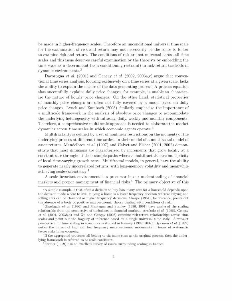
be made in higher-frequency scales. Therefore an unconditional universal time scalefor the examination of risk and return may not necessarily be the route to followto examine risk and return. The conditions of risk are not universal across all timescales and this issue deserves careful examination by the theorists by embedding thetime scale as a determinant (as a conditioning restraint) in risk-return tradeoffs indynamic environments.2

Dacorogna et al. (2001) and Gencay et al. (2002, 2003a,c) argue that conven-tional time series analysis, focusing exclusively on a time series at a given scale, lacksthe ability to explain the nature of the data generating process. A process equationthat successfully explains daily price changes, for example, is unable to character-ize the nature of hourly price changes. On the other hand, statistical propertiesof monthly price changes are often not fully covered by a model based on dailyprice changes. Lynch and Zumbach (2003) similarly emphasize the importance ofa multiscale framework in the analysis of absolute price changes to accommodatethe underlying heterogeneity with intraday, daily, weekly and monthly components.Therefore, a comprehensive multi-scale approach is needed to elaborate the marketdynamics across time scales in which economic agents operate.3

Multifractality is defined by a set of nonlinear restrictions on the moments of theunderlying process at different time-scales. In their model of a multifractal model ofasset returns, Mandelbrot et al. (1997) and Calvet and Fisher (2001, 2002) demon-strate that most diffusions are characterized by increments that grow locally at aconstant rate throughout their sample paths whereas multifractals have multiplicityof local time-varying growth rates. Multifractal models, in general, have the abilityto generate nearly uncorrelated returns, with long-memory volatility and meanwhileachieving scale-consistency.4

A scale invariant environment is a precursor in our understanding of financialmarkets and proper management of financial risks.5 The primary objective of this

2A simple example is that often a decision to buy how many cars for a household depends uponthe decision made where to live. Buying a home is a lower frequency decision whereas buying andselling cars can be classified as higher frequency decisions. Sharpe (1964), for instance, points outthe absence of a body of positive microeconomic theory dealing with conditions of risk.

3Ghashgaie et al. (1996) and Mantegna and Stanley (1996, 1997) have analysed the scalingrelationship from the perspective of turbulence in financial markets. Arneodo et al. (1998), Gencayet al. (2001, 2003b,d) and Xu and Gencay (2003) examine risk-return relationships across timescales and point out the fragility of inference based on a single universal time scale. A waveletperspective for time scaling in economics is studied in Ramsey (1999, 2002). Bjornson et al. (1999)notice the impact of high and low frequency macroeconomic movements in terms of systematicfactor risks in an economy.

4If the aggregated processes all belong to the same class as the original process, then the under-lying framework is referred to as scale consistent.

5Farmer (1999) has an excellent survey of issues surrounding scaling in finance.

2

paper is to obtain a deeper understanding of the underlying multifractal nature offinancial time series towards developing scale invariant models of financial markets.In doing so, we study the scaling laws which govern the data. As noted by Brock(1999), scaling laws are useful because “(i) they stimulate the search for interpre-tive frameworks, (ii) they impose discipline on theory formation (the theory mustgenerate data consistent with the observed scaling results), (iii) (they) give clues tothe properties of the space of possible underlying data generating process.”

This paper is structured as follows. The following section gives a brief descriptionof data and provides some preliminary analysis including intraday stylized facts.Section 3 reports our findings on the multifractal nature of returns and persistenceproperties of large shocks. We conclude afterwards.

2 Data and preliminary analysis

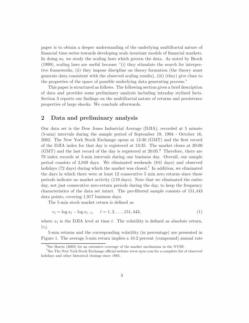
Our data set is the Dow Jones Industrial Average (DJIA), recorded at 5 minute(5-min) intervals during the sample period of September 19, 1994 - October 16,2002. The New York Stock Exchange opens at 13:30 (GMT) and the first recordof the DJIA index for that day is registered at 13:35. The market closes at 20:00(GMT) and the last record of the day is registered at 20:05.6 Therefore, there are79 index records at 5-min intervals during one business day. Overall, our sampleperiod consists of 2,949 days. We eliminated weekends (841 days) and observedholidays (72 days) during which the market was closed.7 In addition, we eliminatedthe days in which there were at least 12 consecutive 5 min zero returns since theseperiods indicate no market activity (119 days). Note that we eliminated the entireday, not just consecutive zero-return periods during the day, to keep the frequencycharacteristics of the data set intact. The pre-filtered sample consists of 151,443data points, covering 1,917 business days.

The 5-min stock market return is defined as

rt = logxt − logxt−1, t = 1, 2, . . . , 151, 443, (1)

where xt is the DJIA level at time t. The volatility is defined as absolute return,|rt|.

5-min returns and the corresponding volatility (in percentage) are presented inFigure 1. The average 5-min return implies a 10.2 percent (compound) annual rate

6See Harris (2003) for an extensive coverage of the market mechanism in the NYSE.7See The New York Stock Exchange official website www.nyse.com for a complete list of observed

holidays and other historical closings since 1885.

3

2000

4000

6000

8000

10000

12000

DJI

A

(a)

−4

−2

0

2

4

6

Ret

urn

(b)

09/94 10/95 11/96 01/98 01/99 02/00 02/01 03/02 03/030

1

2

3

4

5

Time (5−min intervals)

Vol

atili

ty

(c)

Figure 1: Dow Jones Industrial Average at 5-min intervals: (a) DJIA level (b) 5-min return(log difference, in percent) (c) 5-min volatility (absolute return, in percent). Sample periodis September 19, 1994 - October 16, 2002 (151,443 5-mins, 1,917 days). Data source: OlsenGroup (www.olsen.ch).

of return during the sample period.8 The sample statistics indicate that the 5-minstock index return distribution in this frequency is far from being normal. Thesample skewness is 0.68 while the sample kurtosis is 55.2, implying several extremereturns relative to the standard normal distribution. Even if the highest and thelowest 500 5-min returns from the sample are excluded, the sample kurtosis is still5.3. The highest intraday 5-min positive return (4.7 percent on October 28, 1997)is 39 standard deviations (σ) away from the mean while the highest intraday 5-min

8The average 5-min return r5 is 4.71e-006. Assuming 260 business days in one year, the com-pound annual rate of return is given by ry = (1 + r5)

(79×260) − 1 = 0.1016.

4

0 20 40 60 80−0.04

−0.02

0

0.02

0.04

0.06(a)

Lags (5 minutes)

AC

C

00days 05days 10days 15days−0.04

−0.02

0

0.02

0.04

0.06

Lags (5−Min)

(b)

AC

C

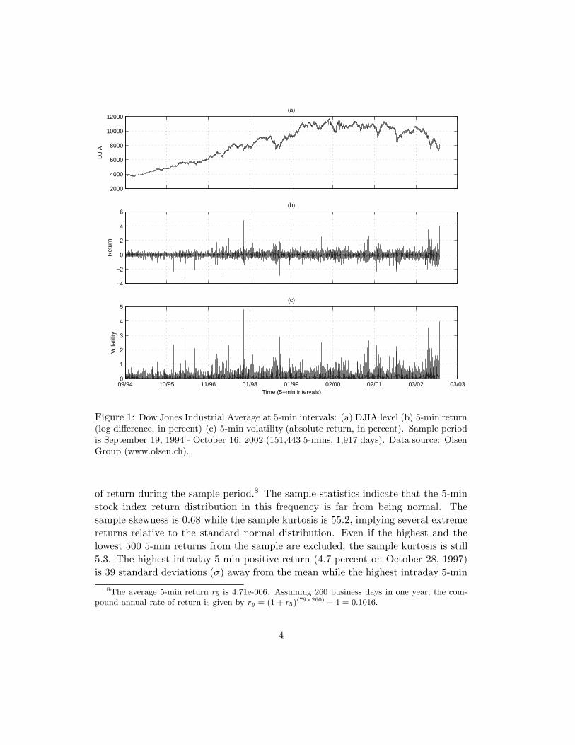
Figure 2: Autocorrelation coefficients (ACC) of the DJIA returns at 5-min lags. (a) Intra-day. (b) 15 days. 95 percent confidence intervals are plotted as solid lines. First two, 42nd(half-day) and 79th (one-day) lag autocorrelation coefficients are statistically significant.One business day consists of 79 5-min intervals (6 hours, 30 minutes). The sample periodis September 19, 1994 - October 16, 2002 (151,443 5-mins, 1,917 days). Data source: OlsenGroup (www.olsen.ch).

negative return (2.9 percent on October 8, 1998) is 24σ. An evaluation of the normalprobability density function shows that the probability of observing a large negativereturn of this size in a normally distributed world would be 10−126.

In Figure 2, the estimated autocorrelation coefficients of returns at 5-min in-tervals are plotted against their lags along with the 95 percent Bartlett confidenceintervals. There is a significant autocorrelation at the first two lags (10-min), the42nd lag (half-day) and the 79th lag (one-day). Other seemingly significant autocor-relation coefficients may be due to sampling deviation. The positive autocorrelationfor daily stock portfolio returns has long been reported in the literature.9 One pos-sible explanation for the first-order positive autocorrelation is the different responsetime of individual stocks to aggregate information (nonsynchronous trading). Astock market index consists of several stocks with different liquidities. One group ofstocks may react to new information more slowly than another group of stocks. Sincethe autocovariance of a well-diversified portfolio is the average of cross-covariancesof individual stocks, significantly positive high-frequency autocorrelations for stockportfolio returns are feasible, (Ahn et al., 2002). It is well known that bid-ask bounce

9See for example, O’Hara (1995), Campbell et al. (1997)[Ch. 2] and Ahn et al. (2002), andreferences therein. More recently, Bouchaud and Potters (2000) have reported significant autocor-relations (up to four lags) of the S&P500 increments measured at 5-min intervals.

5

0 10 20 30 40 50 60 70 80−0.05

0

0.05

0.1

0.15

0.2

0.25

0.3(a)

Lags (5−Min)

AC

Coe

ffici

ent

00days 05days 10days 15days−0.05

0

0.05

0.1

0.15

0.2

0.25

0.3(b)

Lags (5−Min)

AC

Coe

ffici

ent

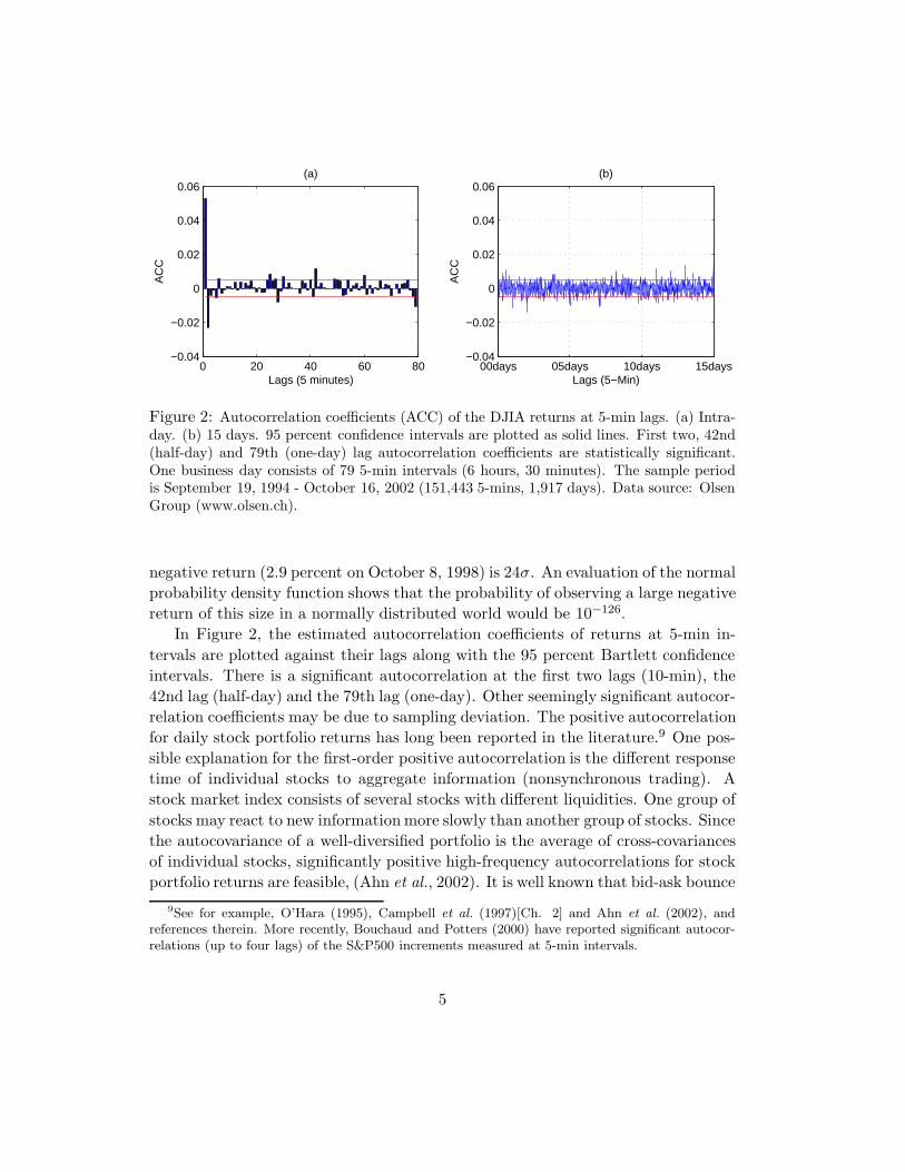
Figure 3: DJIA volatility autocorrelation coefficients at 5-min lags. (a) Intraday. (b) 15days. Volatility is defined as absolute percent return. Notice that there is a strong dailyseasonality. One business day consists of 79 5-min intervals (6 hours and 30 minutes).Sample period is September 19, 1994 - October 16, 2002 (151,443 5-mins, 1,917 days). Datasource: Olsen Group (www.olsen.ch).

leads to negative autocorrelation in stock returns (Roll, 1984). Therefore, one mayargue that the true autocorrelation coefficient may be higher than the one reportedhere.

As illustrated in Figure 3(a), the sample autocorrelation coefficients of 5-minvolatility, defined as absolute returns, are statistically significant, and the intradayautocorrelations have a U shape pattern. The correlation coefficient takes a valueof 23 percent at the first lag and decreases afterwards, reaching a minimum of 10percent at around 2.5 hours lag before starting to rise again. There is a significantpeak at lag 79 which indicates that there is a strong seasonal cycle which completesitself in one day. Figure 3(b) illustrates the autocorrelation coefficients at 5-min lagsup to 15 days. Regarding the weekly seasonality, we do not observe a strong peak at5 days or integer multiple of 5 days. However, this observation should be interpretedwith caution since the presence of daily seasonalities may obscure relatively weakerweekly or longer period seasonal dynamics.

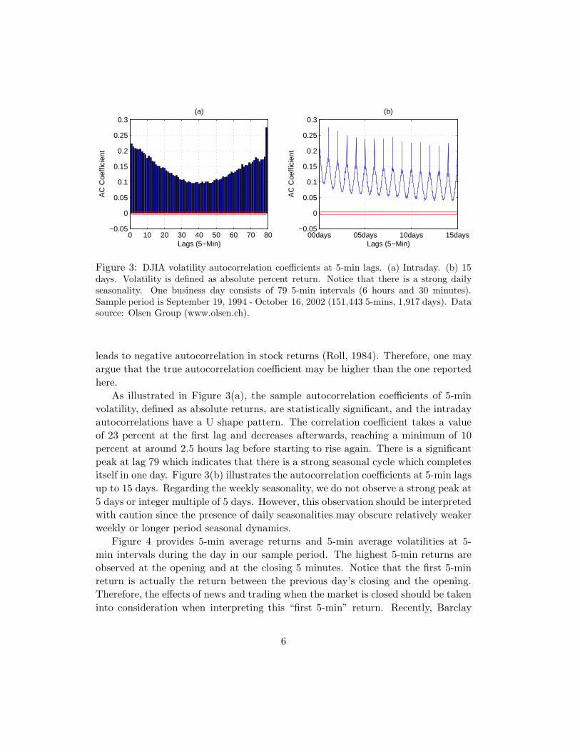
Figure 4 provides 5-min average returns and 5-min average volatilities at 5-min intervals during the day in our sample period. The highest 5-min returns areobserved at the opening and at the closing 5 minutes. Notice that the first 5-minreturn is actually the return between the previous day’s closing and the opening.Therefore, the effects of news and trading when the market is closed should be takeninto consideration when interpreting this “first 5-min” return. Recently, Barclay

6

09:35 10:35 11:35 12:35 01:35 02:35 03:35−0.01

−0.005

0

0.005

0.01

0.015

0.02

0.025

Intraday 5−Min Intervals

Ave

rage

Ret

urn

(Log

Diff

eren

ce),

Per

cent (a)

09:35 10:35 11:35 12:35 01:35 02:35 03:350

0.1

0.2

0.3

0.4

Intraday 5−Min Intervals

Ave

rage

Vol

atili

ty (

Abs

olut

e Lo

g R

etur

n), P

erce

nt

(b)

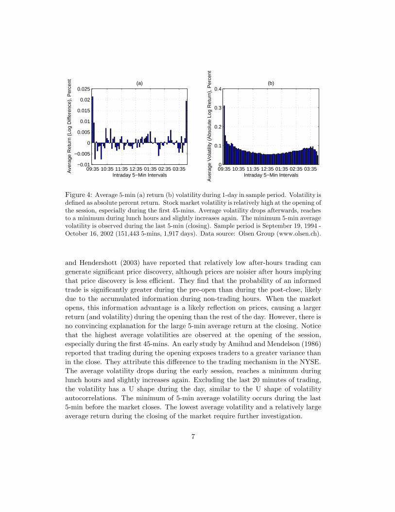
Figure 4: Average 5-min (a) return (b) volatility during 1-day in sample period. Volatility isdefined as absolute percent return. Stock market volatility is relatively high at the opening ofthe session, especially during the first 45-mins. Average volatility drops afterwards, reachesto a minimum during lunch hours and slightly increases again. The minimum 5-min averagevolatility is observed during the last 5-min (closing). Sample period is September 19, 1994 -October 16, 2002 (151,443 5-mins, 1,917 days). Data source: Olsen Group (www.olsen.ch).

and Hendershott (2003) have reported that relatively low after-hours trading cangenerate significant price discovery, although prices are noisier after hours implyingthat price discovery is less efficient. They find that the probability of an informedtrade is significantly greater during the pre-open than during the post-close, likelydue to the accumulated information during non-trading hours. When the marketopens, this information advantage is a likely reflection on prices, causing a largerreturn (and volatility) during the opening than the rest of the day. However, there isno convincing explanation for the large 5-min average return at the closing. Noticethat the highest average volatilities are observed at the opening of the session,especially during the first 45-mins. An early study by Amihud and Mendelson (1986)reported that trading during the opening exposes traders to a greater variance thanin the close. They attribute this difference to the trading mechanism in the NYSE.The average volatility drops during the early session, reaches a minimum duringlunch hours and slightly increases again. Excluding the last 20 minutes of trading,the volatility has a U shape during the day, similar to the U shape of volatilityautocorrelations. The minimum of 5-min average volatility occurs during the last5-min before the market closes. The lowest average volatility and a relatively largeaverage return during the closing of the market require further investigation.

7

3 Scaling Properties

3.1 Scaling of Risk Across Time Scales

A fractal is an object which can be subdivided into parts, each of which is a smallercopy of the whole. Self-similarity, an invariance with respect to scaling, is an im-portant characteristic of fractals. This means that the underlying object is similarat different scales subject to a scaling factor. A stochastic process, [yt] is said to beself-similar if for any positive strectching factor τ , the rescaled process with timescale τt, τ−H [yt]τ , is equal in distribution to the original process [yt],

[yt]τd= τH [yt]. (2)

The Hurst exponent H , also called self-affinity index, or scaling exponent, of [yt],satisfies 0 < H < 1. The operator, d=, indicates that the two probability distribu-tions are equal. This necessitates that samplings at different intervals yield the samedistribution for the process [yt] subject to a scale factor.10 The principle of scaleinvariance suggests an observable relationship between volatilities across differenttime frequencies. Series exhibiting long-term persistence should scale by a factorequivalent to their Hurst exponent which is typically H > 0.5.11 By contrast, arandom walk process scales by the factor H = 0.5. For 0 < H < 0.5, the processhas a short memory.

Rather than being subject to a unique scaling factor, the underlying data gener-ating process may also follow nonlinear forms of scaling. This is where the conceptof multifractals plays an important role in explaining the scaling behavior of severalfinancial time series. In general, we can define an exponent ξ(q) as

E(|[yt]τ |q) = c(q)τ ξ(q) (3)

where E is the expectation operator, q is the order of moments, c(q) and ξ(q) areboth deterministic functions of q. The functions c(q) and ξ(q) are called the scalingfunctions of the multifractal process. Unifractals or uniscaling are a special caseof multifractals where c(q) and ξ(q) are reduced to be linear functions of q. Forexample, ξ(q) = 0.5q for a Gaussian white noise. Multifractal processes, on theother hand, are characterized by the non-linearity of functions c(q) and ξ(q).

10A detailed discussion on self-similarity can be found in Mandelbrot (1977, 1983) and Beran(1994). A self-similar process is also called uniscaling (unifractal). A multiscaling (multifractal)process extends the idea of similarity to allow more general scaling functions. Multifractality isa form of generalized scaling that includes both extreme variations and long-memory. Calvet andFisher (2001, 2002), Matteo et al. (2003, 2004) and Selcuk (2004) have recent findings on theevidence of scaling and multifractality in financial markets.

11The original work on the Hurst exponent is due to Hurst (1951). Later Lo (1991) suggested amodification to eliminate low order persistence.

8

3.2 Empirical Results

Fractal properties of DJIA returns are investigated by studying the 5-min and ag-gregate lower frequency intraday returns. The aggregated returns are defined by

[rt]τ =τ∑

i=1

rτ(t−1)+i, t = 1, . . . , 151, 443/τ (4)

where rt is the original 5-min returns defined in Equation 1, [rt]τ represents thereturns at an aggregated level of τ . For example, the 10-min returns are constructedby summing two 5-min returns where τ = 2. 10-min aggregate returns are definedvia

[rt]2 =2∑

i=1

r2(t−1)+i, t = 1, . . . , 75, 721.

Similarly, lower frequency intraday returns are obtained for different aggregationperiods, τ = 2, 3, . . .12, 24, 36, 48, 60, 72, corresponding to 10 minutes through 6hours of aggregated returns. The last aggregation period corresponds to approxi-mately one business day since the market is open for 6.5 hours (79 5-mins). Thus,the mean moment of absolute returns, for different powers of absolute returns, isexamined at 17 time scales, starting 5-min original returns up to 6 hours, τ =1, 2, 3, . . .12, 24, 36, 48, 60, 72. In our estimations we used the following version ofEquation 3

{E(|[rt]τ |q)}1/q = c(q)τD(q) (5)

where D(q) = ξ(q)/q. We preferred this form so that a fractional Gaussian process(FGN) would result in a constant D(q) for different values of q. For example aGaussian white noise would have D(q) = 0.5 regardless of the choice of q.

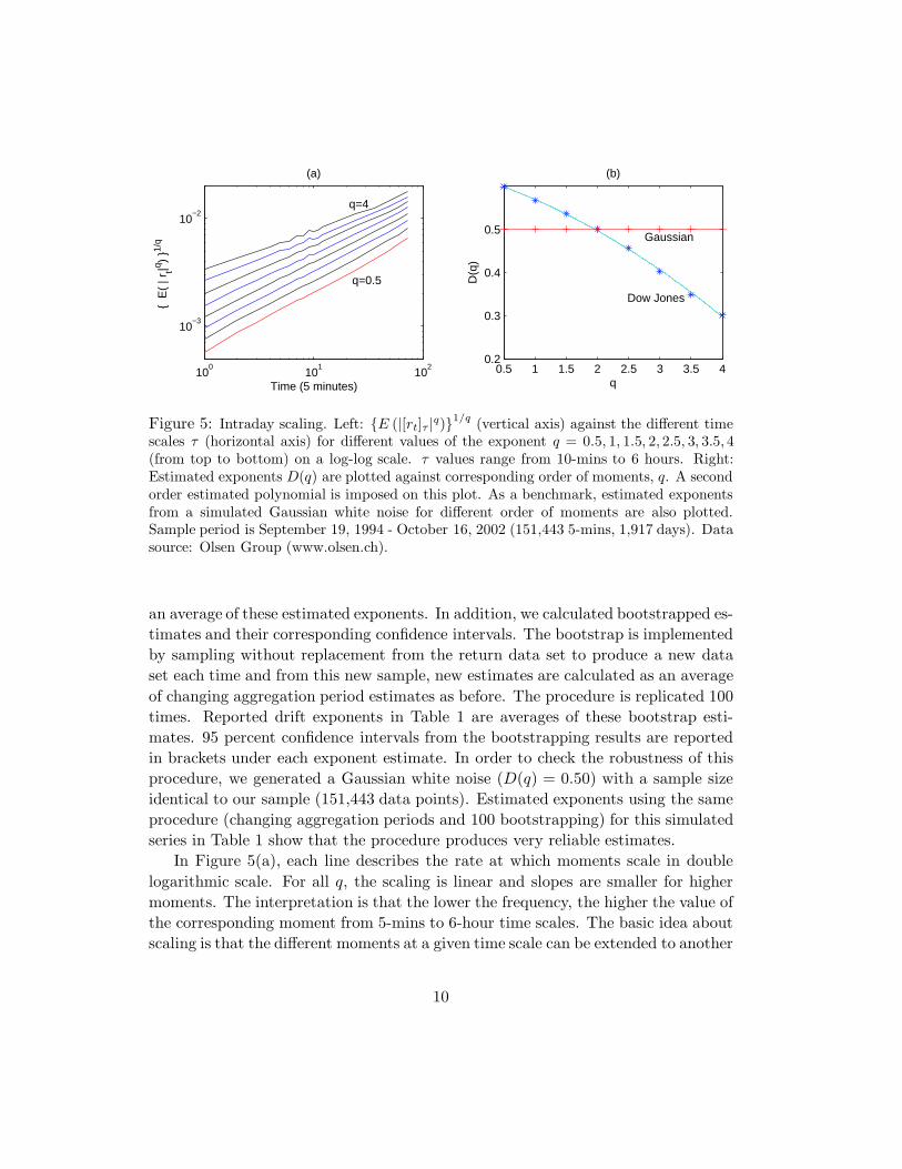
To investigate the multifractal properties of DJIA returns, Figure 5(a) plots{E(|[rt]τ |q)}1/q across 17 time scales for different values of q in a double logarithmicscale. The time intervals range from 5-mins to one day. From bottom to top, thevalues of q increase from 0.5 to 4 at equal increments. The straight lines in thefigure indicate the power scaling law of Equation 5. That is, the qth moment of thereturns subject to a scaling factor when moving from a high-frequency interval tolow-frequency interval.

The estimated exponent D(q) for different values of q in Equation 5 is presentedin Table 1. In order to obtain robust estimates, we changed the highest aggregationfactor τ = 6, 7, . . .12, 24, 36, 48, 60, 72 each time and estimated the exponent D(q)for each aggregation period for different values of q. The final estimate is obtained as

9

100

101

102

10−3

10−2

Time (5 minutes)

{ E

( | r

t|q ) }1/

q

(a)

0.5 1 1.5 2 2.5 3 3.5 40.2

0.3

0.4

0.5

q

D(q

)

(b)

q=0.5

q=4

Gaussian

Dow Jones

Figure 5: Intraday scaling. Left: {E (|[rt]τ |q)}1/q (vertical axis) against the different timescales τ (horizontal axis) for different values of the exponent q = 0.5, 1, 1.5, 2,2.5, 3, 3.5,4(from top to bottom) on a log-log scale. τ values range from 10-mins to 6 hours. Right:Estimated exponents D(q) are plotted against corresponding order of moments, q. A secondorder estimated polynomial is imposed on this plot. As a benchmark, estimated exponentsfrom a simulated Gaussian white noise for different order of moments are also plotted.Sample period is September 19, 1994 - October 16, 2002 (151,443 5-mins, 1,917 days). Datasource: Olsen Group (www.olsen.ch).

an average of these estimated exponents. In addition, we calculated bootstrapped es-timates and their corresponding confidence intervals. The bootstrap is implementedby sampling without replacement from the return data set to produce a new dataset each time and from this new sample, new estimates are calculated as an averageof changing aggregation period estimates as before. The procedure is replicated 100times. Reported drift exponents in Table 1 are averages of these bootstrap esti-mates. 95 percent confidence intervals from the bootstrapping results are reportedin brackets under each exponent estimate. In order to check the robustness of thisprocedure, we generated a Gaussian white noise (D(q) = 0.50) with a sample sizeidentical to our sample (151,443 data points). Estimated exponents using the sameprocedure (changing aggregation periods and 100 bootstrapping) for this simulatedseries in Table 1 show that the procedure produces very reliable estimates.

In Figure 5(a), each line describes the rate at which moments scale in doublelogarithmic scale. For all q, the scaling is linear and slopes are smaller for highermoments. The interpretation is that the lower the frequency, the higher the value ofthe corresponding moment from 5-mins to 6-hour time scales. The basic idea aboutscaling is that the different moments at a given time scale can be extended to another

10

q Dow Jones Simulated FGN

0.5 0.599 0.50[0.595 0.603] [0.494 0.504]

1 0.567 0.50[0.563 0.570] [0.496 0.506]

1.5 0.536 0.50[0.531 0.540] [0.495 0.504]

2 0.50 0.50[0.496 0.503] [0.496 0.506]

2.5 0.456 0.50[0.451 0.461] [0.495 0.504]

3 0.403 0.50[0.397 0.411] [0.495 0.505]

3.5 0.349 0.50[0.339 0.357] [0.495 0.505]

4 0.30 0.50[0.286 0.312] [0.495 0.504]

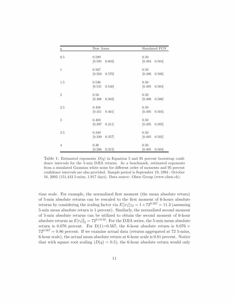
Table 1: Estimated exponents D(q) in Equation 5 and 95 percent bootstrap confi-dence intervals for the 5-min DJIA returns. As a benchmark, estimated exponentsfrom a simulated Gaussian white noise for different order of moments and 95 percentconfidence intervals are also provided. Sample period is September 19, 1994 - October16, 2002 (151,443 5-mins, 1,917 days). Data source: Olsen Group (www.olsen.ch).

time scale. For example, the normalized first moment (the mean absolute return)of 5-min absolute returns can be rescaled to the first moment of 6-hours absolutereturns by considering the scaling factor via E[|rt|]72 = 1×720.567 = 11.3 (assuming5-min mean absolute return is 1 percent). Similarly, the normalized second momentof 5-min absolute returns can be utilized to obtain the second moment of 6-hourabsolute returns as E|rt|272 = 722×0.50. For the DJIA series, the 5-min mean absolutereturn is 0.076 percent. For D(1)=0.567, the 6-hour absolute return is 0.076 ×720.567 = 0.86 percent. If we examine actual data (returns aggregated at 72 5-mins,6-hour scale), the actual mean absolute return at 6-hour scale is 0.81 percent. Noticethat with square root scaling (D(q) = 0.5), the 6-hour absolute return would only

11

be 0.64 percent (0.076× 720.5).The estimation results indicate different exponents D(q) for different values of q

in Equation 5, which suggest that there are different scaling laws for different orderof moments. The lower moments of absolute returns scale faster than the highermoments. Particularly, the moments up to q = 2 scale faster than a Gaussian whitenoise while the moments greater than 2 (q > 2) scale slower than a Gaussian whitenoise. The second moment q = 2 appears to be the borderline. For example, supposethat the normalized mean absolute return is 1 percent. If we assume a Gaussianwhite noise, the corresponding 6-hour mean absolute return would be 720.50 = 8.5percent while the estimated exponent implies 720.567 = 11.3 percent mean absolutereturn at the 6-hour scale. Notice that higher moments of the absolute returnsgive more weight to large observations (tails of the empirical distribution). Similarresults are obtained earlier in the literature. By employing Equation 5 in theirestimations, Dacorogna et al. (2001) report D(1) around 0.60 and D(2) at around0.50 for major foreign exchanges and Eurofutures. Similarly, Selcuk (2004) reportsthat the estimated D(1) is in between 0.55 and 0.59, D(2) is around 0.50 and thehigher moments have D(q) less than 0.50.

Recall that the return process is monofractal if ξ(q) = qξ(1) is a linear functionof q and multifractal if ξ(q) is nonlinear function of q. To illustrate, the estimatedexponent D(q) is plotted against q along with estimated D(q) from a Gaussian whitenoise in Figure 5(b). The exponent D(q) for the Gaussian white noise stays constantat 0.5 as expected while the estimated exponents from 5-min Dow Jones return seriesstart with 0.6 at q = 0.5 and fall to 0.3 at q = 4, suggesting multifractal behaviorof the return process. An estimated second order polynomial for the estimatedexponents D(q) in Figure 5(b) is

y = −0.0023q2 − 0.023q + 0.62

where y is the estimated exponent. Clearly, D(q) is non-linear and the non-linearityof D(q) verifies that the DJIA return process is multifractal.

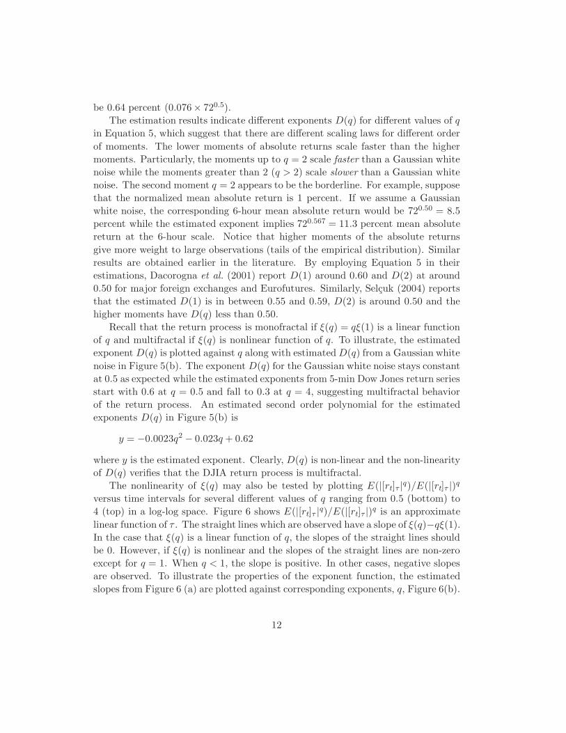
The nonlinearity of ξ(q) may also be tested by plotting E(|[rt]τ |q)/E(|[rt]τ |)q

versus time intervals for several different values of q ranging from 0.5 (bottom) to4 (top) in a log-log space. Figure 6 shows E(|[rt]τ |q)/E(|[rt]τ |)q is an approximatelinear function of τ . The straight lines which are observed have a slope of ξ(q)−qξ(1).In the case that ξ(q) is a linear function of q, the slopes of the straight lines shouldbe 0. However, if ξ(q) is nonlinear and the slopes of the straight lines are non-zeroexcept for q = 1. When q < 1, the slope is positive. In other cases, negative slopesare observed. To illustrate the properties of the exponent function, the estimatedslopes from Figure 6 (a) are plotted against corresponding exponents, q, Figure 6(b).

12

100

101

102

10−1

100

101

102

103

Time (5 minutes)

E(

| [r t] τ| q )

/ E(

| [r t] τ|)

q

(a)

0 1 2 3 4−0.8

−0.6

−0.4

−0.2

0

0.2

q

Slo

pe

(b)

q=4

q=0.5

Figure 6: Intraday scaling. Left: E (|[rt]τ |q) /E (|[rt]τ |)q (vertical axis) against thedifferent time intervals τ (horizontal axis) for different values of the exponent q =0.5, 1, 1.5,2,2.5, 3,3.5, 4 (from bottom to top) on a log-log scale. Right: Estimated slopesfrom the left panel against corresponding exponent, q. A second order polynomial fit isimposed on this plot. Sample period is September 19, 1994 - October 16, 2002 (151,4435-mins, 1,917 days). Data source: Olsen Group (www.olsen.ch).

The estimated second order polynomial in this case is

y = −0.07q2 + 0.13q − 0.054

where y is the estimated slope coefficient. Once again, it is evident that ξ(q) isa nonlinear function of q, which provides further evidence that the DJIA returnprocess is multifractal.12

3.3 Financial Earthquakes and Aftershocks

Mandelbrot (1963a,b) eloquently demonstrated the importance of Pareto’s law forthe power decay of the tails of return distributions.13 Although the tails of returndistributions follow a power law at high frequency scales, this decay does not takethe time order into account. The time path followed by these shocks is an identifyingfactor for a model of returns. Along with Sornette et al. (1996), Lillo and Mantegna

12Bouchaud et al. (2000) show that multiscaling can be observed as a result of a slow crossoverphenomenon on a finite time event although the underlying process is a monofractal. They warnthat it might be hard to distinguish apparent and true multifractal behavior in financial data.

13LeBaron (2001), Mandelbrot (2001) and Stanley and Plerou (2001) discuss whether stochasticvolatility models follow a power law behavior.

13

(2002, 2003) and Selcuk (2004), we examine the persistence of shocks in intradayscales.

A major earthquake in a region is usually followed by smaller ones, labeled as“aftershocks”. There are several approaches to describe the dynamics of aftershocks.A well-known simple rule is the Gutenberg-Richter relation, which says that thenumber of earthquakes of magnitude M or greater, N(M), is given by

log10 N(M) = a − bM (6)

where a and b are two constants. In several studies, b is found to be within therange of 0.7 to 1 regionally. However, for larger geographical areas and the world,the slope parameter is usually 1. The interpretation is such that we will observeapproximately ten times as many aftershocks with a magnitude one unit less thanthe main shock. Fitting the tail of a distribution in finance is analogous to thisrelationship.

Another approach relates the time after the main shock to the number of after-shocks per unit time, n(t). This is known as the Omori law.14 Omori’s law statesthat the number of aftershocks per unit time decays according to the power law oft−p. In order to avoid divergence at t = 0, Omori’s law is rewritten as

n(t) = K(t + τ)−p (7)

where K and τ are constants. By integrating Equation 7 between 0 and t, thecumulative number of aftershocks between the main shock and the time t can beexpressed as

N(t) = K[(t + τ)1−p − τ1−p

]/(1 − p) (8)

when p 6= 1 and N(t) = K ln(t/1 + τ) for p = 1 (Lillo and Mantegna, 2002).By performing numerical simulations and theoretical modeling, Lillo and Man-

tegna (2002) show that the nonlinear behavior observed in real market crashes can-not be described by popular volatility models. Particularly, they show that simu-lated GARCH(1,1) time series converges to its stationary phase very quickly aftera large shock and it is unable to show a significant nonlinear behavior. Recently, aseries of papers has investigated the behavior of volatility in financial markets afterbig crashes. An early work by Sornette et al. (1996) shows that the implied volatilityin the S&P500 after the 1987 financial crash has a power law-periodic decay. Lilloand Mantegna (2002, 2003) have shown that S&P500 index returns above a largethreshold are well described by a power law function which is analogous to Omori’s

14See Omori (1894), Lillo and Mantegna (2002) and Lillo and Mantegna (2003).

14

00 05 10 15 20 25 300

10

20

30

40

50

60

Days

Cum

ulat

ive

Sho

cks

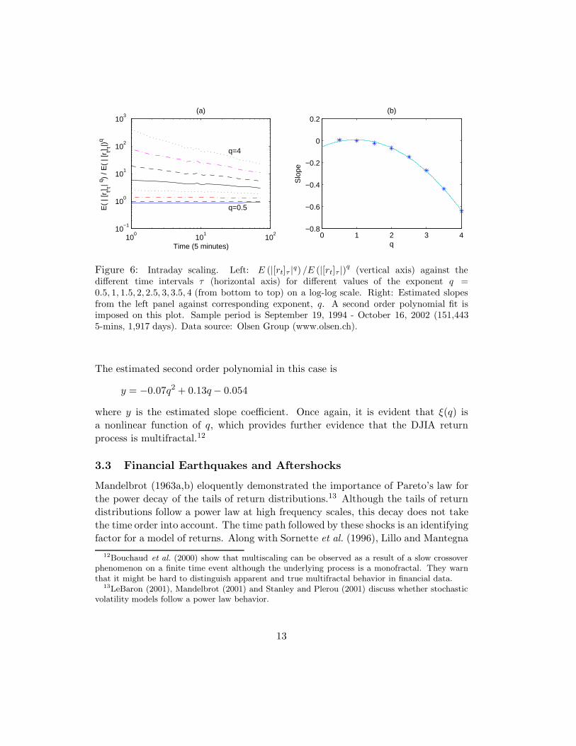
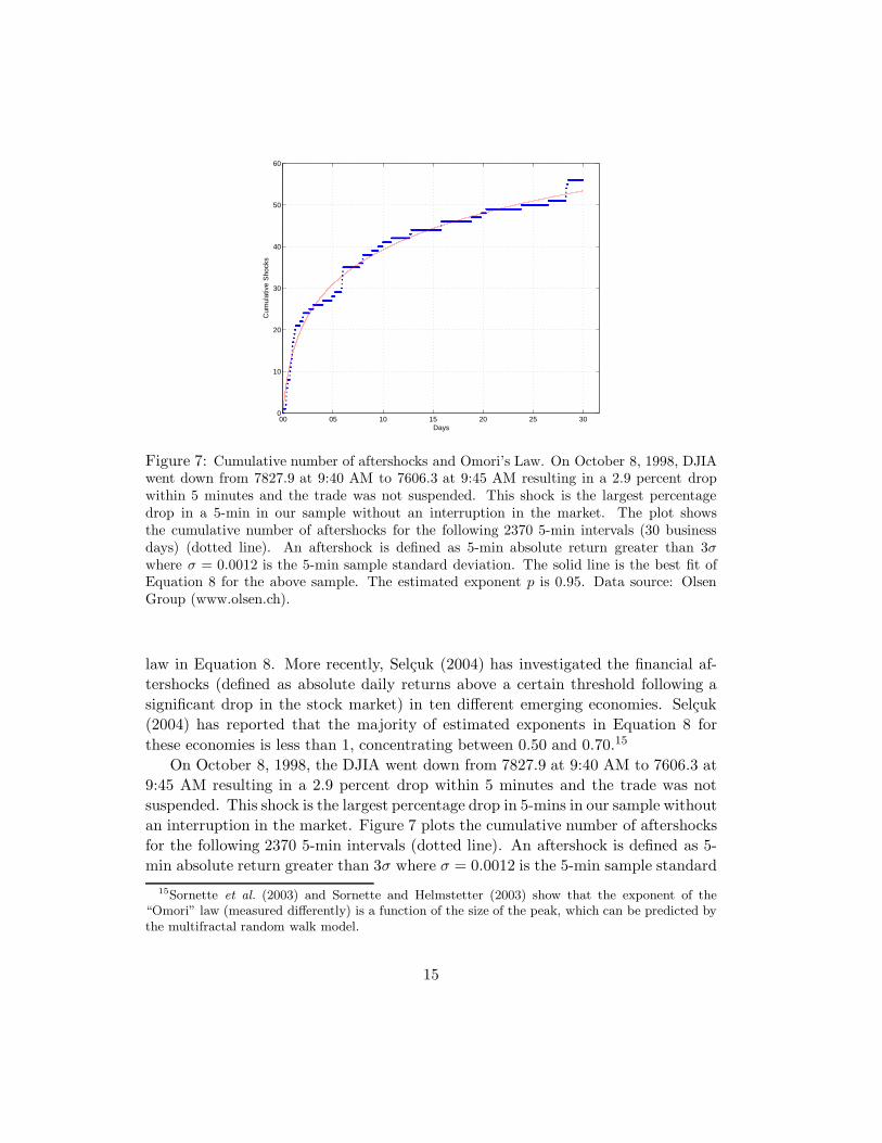
Figure 7: Cumulative number of aftershocks and Omori’s Law. On October 8, 1998, DJIAwent down from 7827.9 at 9:40 AM to 7606.3 at 9:45 AM resulting in a 2.9 percent dropwithin 5 minutes and the trade was not suspended. This shock is the largest percentagedrop in a 5-min in our sample without an interruption in the market. The plot showsthe cumulative number of aftershocks for the following 2370 5-min intervals (30 businessdays) (dotted line). An aftershock is defined as 5-min absolute return greater than 3σwhere σ = 0.0012 is the 5-min sample standard deviation. The solid line is the best fit ofEquation 8 for the above sample. The estimated exponent p is 0.95. Data source: OlsenGroup (www.olsen.ch).

law in Equation 8. More recently, Selcuk (2004) has investigated the financial af-tershocks (defined as absolute daily returns above a certain threshold following asignificant drop in the stock market) in ten different emerging economies. Selcuk(2004) has reported that the majority of estimated exponents in Equation 8 forthese economies is less than 1, concentrating between 0.50 and 0.70.15

On October 8, 1998, the DJIA went down from 7827.9 at 9:40 AM to 7606.3 at9:45 AM resulting in a 2.9 percent drop within 5 minutes and the trade was notsuspended. This shock is the largest percentage drop in 5-mins in our sample withoutan interruption in the market. Figure 7 plots the cumulative number of aftershocksfor the following 2370 5-min intervals (dotted line). An aftershock is defined as 5-min absolute return greater than 3σ where σ = 0.0012 is the 5-min sample standard

15Sornette et al. (2003) and Sornette and Helmstetter (2003) show that the exponent of the“Omori” law (measured differently) is a function of the size of the peak, which can be predicted bythe multifractal random walk model.

15

00 05 10 15 20 25 300

2

4

6

8

10

12

14

16

18

Days

Cum

ulat

ive

Sho

cks

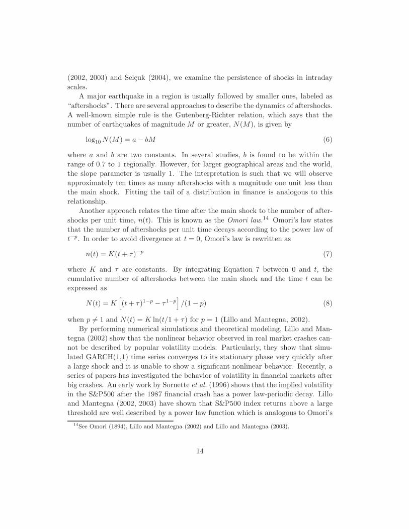
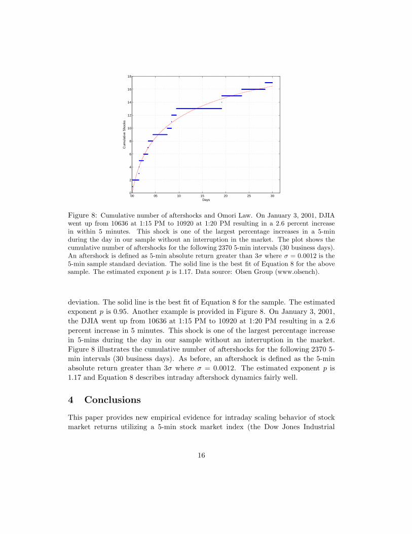
Figure 8: Cumulative number of aftershocks and Omori Law. On January 3, 2001, DJIAwent up from 10636 at 1:15 PM to 10920 at 1:20 PM resulting in a 2.6 percent increasein within 5 minutes. This shock is one of the largest percentage increases in a 5-minduring the day in our sample without an interruption in the market. The plot shows thecumulative number of aftershocks for the following 2370 5-min intervals (30 business days).An aftershock is defined as 5-min absolute return greater than 3σ where σ = 0.0012 is the5-min sample standard deviation. The solid line is the best fit of Equation 8 for the abovesample. The estimated exponent p is 1.17. Data source: Olsen Group (www.olsench).

deviation. The solid line is the best fit of Equation 8 for the sample. The estimatedexponent p is 0.95. Another example is provided in Figure 8. On January 3, 2001,the DJIA went up from 10636 at 1:15 PM to 10920 at 1:20 PM resulting in a 2.6percent increase in 5 minutes. This shock is one of the largest percentage increasein 5-mins during the day in our sample without an interruption in the market.Figure 8 illustrates the cumulative number of aftershocks for the following 2370 5-min intervals (30 business days). As before, an aftershock is defined as the 5-minabsolute return greater than 3σ where σ = 0.0012. The estimated exponent p is1.17 and Equation 8 describes intraday aftershock dynamics fairly well.

4 Conclusions

This paper provides new empirical evidence for intraday scaling behavior of stockmarket returns utilizing a 5-min stock market index (the Dow Jones Industrial

16

Average) from the New York Stock Exchange. Our findings indicate that the returngenerating process cannot be explained by a single data generating process (DGP)due to the fact that there is no unique DGP under a model of returns. Hence, forinstance, there is no unique volatility measure belonging to a unique DGP undera model. In fact, under a model, the DGP of returns is multifractal consistingof infinitely many DGPs. Furthermore, it is not certain whether the statisticalinference from the existing return/volatility literature can be classified as pivotal.In addition, we show that after a financial “earthquake”, aftershocks in the marketfollow a power law, analogous to Omori’s law. This nonlinear behavior observed inreal market crashes cannot be described by popular volatility models.

17

References

Ahn, D., Boudoukh, J., Richardson, M., and Whitelaw, R. F. (2002). Partial ad-justment or stale prices? Implications from stock index and futures return auto-correlations. Review of Financial Studies, 15, 655–689.

Amihud, Y. and Mendelson, H. (1986). Trading mechanisms and stock returns: Anempirical investigation. Journal of Finance, 42, 533–553.

Arneodo, A., Muzy, J. F., and Sornette, D. (1998). “Direct” causal cascade in thestock market. European Physical Journal B, 2, 277–282.

Barclay, M. J. and Hendershott, T. (2003). Price discovery and trading after hours.Review of Financial Studies, 16, 1041–1073.

Beran, J. (1994). Statistics for Long-Memory Processes. London: Chapman & Hall.

Bjornson, B., Kim, H. S., and Lee, K. (1999). Low and high frequency macroeco-nomic forces in asset pricing. Quarterly Review of Economics and Finance, 39,77–100.

Bouchaud, J. P. and Potters, M. (2000). Theory of Financial Risks: From StatisticalPhysics to Risk Management. Cambridge University Press, Cambridge, UK.

Bouchaud, J. P., Potters, M., and Meyer, M. (2000). Apparent multifractality infinancial time series. European Physical Journal B, 13, 595–599.

Brock, W. A. (1999). Scaling in economics: A reader’s guide. Industrial and Cor-porate Change, 8, 409–446.

Calvet, L. and Fisher, A. (2001). Forecasting multifractal volatility. Journal ofEconometrics, 105, 27–58.

Calvet, L. and Fisher, A. (2002). Multifractality in asset returns: Theory andevidence. Review of Economics and Statistics, 84, 381–406.

Campbell, J. Y. (2000). Asset pricing at the millennium. Journal of Finance, 4,1515–1567.

Campbell, J. Y., Lo, A. W., and MacKinlay, A. C. (1997). The Econometrics ofFinancial Markets. Princeton University Press, Princeton, NJ.

Cochrane, J. H. (1999). New facts in finance. Federal Reserve Bank of Chicago, 23,59–78.

18

Dacorogna, M., Gencay, R., Muller, U., Olsen, R., and Pictet, O. (2001). AnIntroduction to High-Frequency Finance. Academic Press, San Diego.

Davidson, R. and MacKinnon, J. G. (2003). Econometric Theory and Methods. NewYork: Oxford Press.

Farmer, J. D. (1999). Physicists attempt to scale the ivory towers of finance. Com-puting in Science and Engineering (IEEE), November/December, 26–39.

Gencay, R., Selcuk, F., and Whitcher, B. (2001). An Introduction to Wavelets andOther Filtering Methods in Finance and Economics. Academic Press, San Diego.

Gencay, R., , Ballocchi, G., Dacorogna, M., Olsen, R., and Pictet, O. (2002). Real-time trading models and the statistical properties of foreign exchange rates. In-ternational Economic Review, 43, 463–491.

Gencay, R., Selcuk, F., and Whitcher, B. (2003a). Asymmetry ofinformation flow between volatilities across time scales. Manuscript,http://carleton.ca/∼rgencay/whmm.pdf.

Gencay, R., Selcuk, F., and Whitcher, B. (2003b). Multiscale systematic risk. Jour-nal of International Money and Finance, (forthcoming).

Gencay, R., , Dacorogna, M., Olsen, R., and Pictet, O. (2003c). Real-time tradingmodels and market behavior. Journal of Economic Dynamic and Control, 27,909–935.

Gencay, R., Selcuk, F., and Whitcher, B. (2003d). Systematic risk and time scales.Quantitative Finance, 3, 108–116.

Ghashgaie, S., Breymann, W., Peinke, J., Talkner, P., and Dodge, Y. (1996). Tur-bulent cascades in foreign exchange markets. Nature, 381, 767–770.

Harris, L. (2003). Trading&Exchanges: Market Microstructure for Practitioners.Oxford University Press, Oxford.

Hurst, H. E. (1951). Long-term storage capacity of reservoirs. Transactions of theAmerican Society of Civil Engineers, 116, 770–799.

LeBaron, B. (2001). Stochastic volatility as a simple generator of apparent financialpower laws and long memory. Quantitative Finance, 1, 621–631.

Lillo, F. and Mantegna, R. N. (2002). Dynamics of financial market index after acrash. Manuscript, http://arXiv.org/abs/cond-mat/0209685.

19

Lillo, F. and Mantegna, R. N. (2003). Power law relaxation in a complex system:Omori law after a financial market crash. Physical Review E, 68, 1–5.

Lo, A. W. (1991). Long-memory in stock market prices. Econometrica, 59, 1279–1313.

Lynch, P. E. and Zumbach, G. O. (2003). Market heterogeneities and the causalstructure of volatility. Quantitative Finance, 3, 320–331.

Mandelbrot, B., Fisher, A., and Calvet, L. (1997). A multifractal model of assetreturns. Cowles Foundation Discussion Paper No. 1164, Yale University.

Mandelbrot, B. B. (1963a). New methods in statistical economics. Journal ofPolitical Economy, 71, 421–440.

Mandelbrot, B. B. (1963b). The variation of certain speculative prices. Journal ofBusiness, 36, 394–419.

Mandelbrot, B. B. (1977). Fractals, Form, Chance and Dimension. New York:W. H. Freeman and Company.

Mandelbrot, B. B. (1983). The Fractal Geometry of Nature. New York: W. H.Freeman and Company.

Mandelbrot, B. B. (2001). Stochastic volatility, power laws and long memory. Quan-titative Finance, 6, 558–559.

Mantegna, R. N. and Stanley, H. E. (1996). Turbulent and exchange markets.Nature, 383, 587–588.

Mantegna, R. N. and Stanley, H. E. (1997). Stock market dynamics and turbulence:Parallel analysis of fluctuation phenomena. Physica A, 239, 255–266.

Matteo, T. D., Aste, T., and Dacorogna, M. M. (2003). Scaling behaviors in differ-ently developed markets. Physica A, 324, 183–188.

Matteo, T. D., Aste, T., and Dacorogna, M. M. (2004). Using the scaling analysisto characterize financial markets. Journal of Empirical Finance, (forthcoming).

O’Hara, M. (1995). Market Microstructure Theory. Blackwell Publishers Ltd, Ox-ford.

Omori, F. (1894). On the after-shocks of earthquakes. J. Coll. Sci. Imp. Univ.Tokyo, 7, 111–200.

20

Poon, S. and Granger, C. W. J. (2003). Forecasting volatility in financial markets:A review. Journal of Economic Literature, 41, 478–539.

Ramsey, J. B. (1999). The contribution of wavelets to the analysis of economic andfinancial data. Philosophical Transactions of the Royal Society of London A, 357,2593–2606.

Ramsey, J. B. (2002). Wavelets in economics and finance: Past and future. Studiesin Nonlinear Dynamics & Econometrics, 3, 1.

Roll, R. (1984). A simple implicit measure of the effective bid-ask spread in anefficient market. Journal of Finance, 39, 1127–1139.

Selcuk, F. (2004). Financial earthquakes, aftershocks and scaling in emerging stockmarkets. Physica A, (forthcoming).

Sharpe, W. F. (1964). Capital asset prices: a theory of market equilibrium underconditions of risk. Journal of Finance, 19, 425–442.

Sornette, D. and Helmstetter, A. (2003). Endogeneous versus exogeneous shocks insystems with memory. Physica A, 318, 577–591.

Sornette, D., Johansen, A., and Bouchaud, J. P. (1996). Stock market crashes,precursors and replicas. Journal de Physique I, 6, 167–175.

Sornette, D., Malevergne, Y., and Muzy, J. F. (2003). What causes crashes? Risk,16, 67–71.

Stanley, H. E. and Plerou, V. (2001). Scaling and universality in economics: Em-pirical results and theoretical interpretation. Quantitative Finance, 1, 563–567.

Xu, Z. and Gencay, R. (2003). Scaling, self-similarity and multifractality in FXmarkets. Physica A, 323, 578–590.

21