Intra Prediction Based on Markov Process Modeling of Images

3916 IEEE TRANSACTIONS ON IMAGE PROCESSING, VOL. 22, NO. 10, OCTOBER 2013

Intra Prediction Based on Markov ProcessModeling of Images

Fatih Kamisli, Member, IEEE

Abstract— In recent video coding standards, intraprediction ofa block of pixels is performed by copying neighbor pixels of theblock along an angular direction inside the block. Each blockpixel is predicted from only one or few directionally alignedneighbor pixels of the block. Although this is a computationallyefficient approach, it ignores potentially useful correlation ofother neighbor pixels of the block. To use this correlation, ageneral linear prediction approach is proposed, where each blockpixel is predicted using a weighted sum of all neighbor pixels ofthe block. The disadvantage of this approach is the increasedcomplexity because of the large number of weights. In thispaper, we propose an alternative approach to intraprediction,where we model image pixels with a Markov process. TheMarkov process model accounts for the ignored correlationin standard intraprediction methods, but uses few neighborpixels and enables a computationally efficient recursive predictionalgorithm. Compared with the general linear prediction approachthat has a large number of independent weights, the Markovprocess modeling approach uses a much smaller number ofindependent parameters and thus offers significantly reducedmemory or computation requirements, while achieving similarcoding gains with offline computed parameters.

Index Terms— Image coding, video coding, markov processes,prediction methods.

I. INTRODUCTION

INTRA prediction is an important tool of modern intra-frame coding. In intra-frame coding with intra prediction,

a block of pixels is first predicted from its neighbor pixelsin previously coded blocks, and then the prediction error istransform-coded.

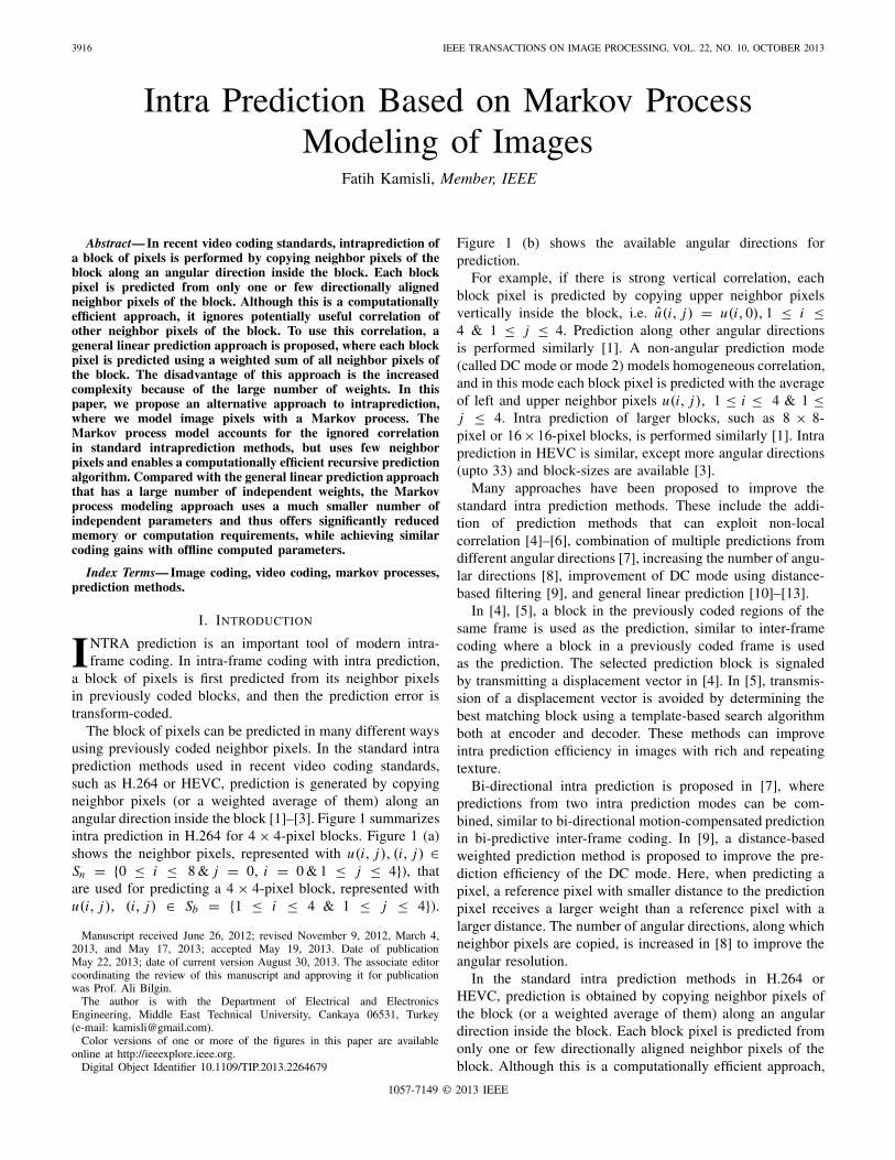
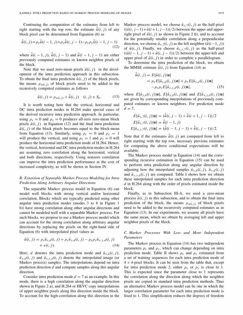
The block of pixels can be predicted in many different waysusing previously coded neighbor pixels. In the standard intraprediction methods used in recent video coding standards,such as H.264 or HEVC, prediction is generated by copyingneighbor pixels (or a weighted average of them) along anangular direction inside the block [1]–[3]. Figure 1 summarizesintra prediction in H.264 for 4 × 4-pixel blocks. Figure 1 (a)shows the neighbor pixels, represented with u(i, j), (i, j) ∈Sn = {0 ≤ i ≤ 8 & j = 0, i = 0 & 1 ≤ j ≤ 4}), thatare used for predicting a 4 × 4-pixel block, represented withu(i, j), (i, j) ∈ Sb = {1 ≤ i ≤ 4 & 1 ≤ j ≤ 4}).

Manuscript received June 26, 2012; revised November 9, 2012, March 4,2013, and May 17, 2013; accepted May 19, 2013. Date of publicationMay 22, 2013; date of current version August 30, 2013. The associate editorcoordinating the review of this manuscript and approving it for publicationwas Prof. Ali Bilgin.

The author is with the Department of Electrical and ElectronicsEngineering, Middle East Technical University, Cankaya 06531, Turkey(e-mail: [email protected]).

Color versions of one or more of the figures in this paper are availableonline at http://ieeexplore.ieee.org.

Digital Object Identifier 10.1109/TIP.2013.2264679

Figure 1 (b) shows the available angular directions forprediction.

For example, if there is strong vertical correlation, eachblock pixel is predicted by copying upper neighbor pixelsvertically inside the block, i.e. u(i, j) = u(i, 0), 1 ≤ i ≤4 & 1 ≤ j ≤ 4. Prediction along other angular directionsis performed similarly [1]. A non-angular prediction mode(called DC mode or mode 2) models homogeneous correlation,and in this mode each block pixel is predicted with the averageof left and upper neighbor pixels u(i, j), 1 ≤ i ≤ 4 & 1 ≤j ≤ 4. Intra prediction of larger blocks, such as 8 × 8-pixel or 16 ×16-pixel blocks, is performed similarly [1]. Intraprediction in HEVC is similar, except more angular directions(upto 33) and block-sizes are available [3].

Many approaches have been proposed to improve thestandard intra prediction methods. These include the addi-tion of prediction methods that can exploit non-localcorrelation [4]–[6], combination of multiple predictions fromdifferent angular directions [7], increasing the number of angu-lar directions [8], improvement of DC mode using distance-based filtering [9], and general linear prediction [10]–[13].

In [4], [5], a block in the previously coded regions of thesame frame is used as the prediction, similar to inter-framecoding where a block in a previously coded frame is usedas the prediction. The selected prediction block is signaledby transmitting a displacement vector in [4]. In [5], transmis-sion of a displacement vector is avoided by determining thebest matching block using a template-based search algorithmboth at encoder and decoder. These methods can improveintra prediction efficiency in images with rich and repeatingtexture.

Bi-directional intra prediction is proposed in [7], wherepredictions from two intra prediction modes can be com-bined, similar to bi-directional motion-compensated predictionin bi-predictive inter-frame coding. In [9], a distance-basedweighted prediction method is proposed to improve the pre-diction efficiency of the DC mode. Here, when predicting apixel, a reference pixel with smaller distance to the predictionpixel receives a larger weight than a reference pixel with alarger distance. The number of angular directions, along whichneighbor pixels are copied, is increased in [8] to improve theangular resolution.

In the standard intra prediction methods in H.264 orHEVC, prediction is obtained by copying neighbor pixels ofthe block (or a weighted average of them) along an angulardirection inside the block. Each block pixel is predicted fromonly one or few directionally aligned neighbor pixels of theblock. Although this is a computationally efficient approach,

1057-7149 © 2013 IEEE

KAMISLI: INTRA PREDICTION BASED ON MARKOV PROCESS MODELING OF IMAGES 3917

Fig. 1. Intra prediction in H.264 for 4 × 4-pixel blocks. (a) Neighbor pixels u(i, j), (i, j) ∈ Sn = {0 ≤ i ≤ 8 & j = 0, i = 0 & 1 ≤ j ≤ 4} are used forintra prediction of a 4 × 4-pixel block u(i, j), (i, j) ∈ Sb = {1 ≤ i ≤ 4 & 1 ≤ j ≤ 4}. (b) Available angular directions.

it ignores potentially useful information in other neighborpixels of the block. To utilize this information, a generallinear prediction approach has been proposed [10]–[13].In this approach, each block pixel is predicted using aweighted sum of all neighbor pixels of the block. The weightschange depending on the location of the prediction pixelinside the block and the angular direction of prediction, andtherefore a large number of weights are required in the linearprediction approach. The linear prediction weights can bedetermined offline or online. In the offline approaches, a largeamount of memory is required at the encoder and decoder tostore the offline computed weights. In the online approaches,large amounts of computations are required at the encoderand decoder to compute the weights online during encodingand decoding.

In this paper, we propose an alternative approach to intraprediction, where we model image pixels with a Markovprocess. The Markov process model accounts for the ignoredcorrelation of standard intra prediction methods, but uses fewneighbor pixels and enables a computationally efficient recur-sive prediction algorithm. At each iteration of the recursion,the same weights, which are obtained from few independentparameters of the Markov process model, are used. Comparedto the large number of independent weights of the linearprediction approach, the Markov process modeling approachuses much smaller number of independent parameters andthus offers significantly reduced memory or computationrequirements, while achieving similar coding gains with offlinecomputed parameters.

The remainder of the paper is organized as follows.In Section II, we review the linear prediction approach andthe least-squares method for determining the linear predic-tion weights. In Section III, we present the intra predictionapproach based on Markov process modeling of images.We use several Markov process models with varying numberof independent parameters, and compare the number of inde-pendent parameters of these models and the linear predictionapproach. In Section IV, we provide experimental results andSection V concludes the paper. We carry out the discussionin the paper using 4 × 4-pixel blocks and the intra predictiondirections in H.264, but the discussion can be easily extendedto other block-sizes and angular directions such as thosein HEVC. The experimental results are also provided bymodifying the reference software of H.264. Some preliminaryresults of this work appear in [14].

II. LINEAR PREDICTION APPROACH

A. Linear Prediction Approach and the Least-Squares Methodfor Obtaining the Linear Prediction Weights

The angular copying of neighbor pixels is a computationallyefficient special case of a general linear prediction approach,where each block pixel u(i, j), (i, j) ∈ Sb is predicted by aweighted sum of all neighbor pixels u(i, j), (i, j) ∈ Sn ofthe block (see Figure 1). The weights of the neighbor pixelschange depending on the location (i, j) of the predicted pixeland the prediction direction d . In vector notation, the linearprediction approach can be represented as follows:

ud(i, j) = nT · wd,i, j , (i, j) ∈ Sb, d = 0..8 (1)

where ud (i, j) represents the linear prediction of block pixelat location (i, j) using prediction direction d , n representsa column vector1 of neighbor pixels, and wd,i, j representsa column vector1 of weights associated with those neighborpixels.

An important part of this approach is the determination ofthe used weights wd,i, j . A common approach to determinethese weights is to solve an overdetermined linear system ofthe weights, obtained from previously coded data, for its least-squares solution [10]–[13]. The overdetermined linear systemcan be expressed as

ud,i, j = Nd · wd,i, j , (i, j) ∈ Sb, d = 0..8 (2)

where ud,i, j is a column vector of size M containing Msamples of block pixel u(i, j) from blocks previously codedwith angular prediction direction d , Nd is a tall matrix of sizeMx13 containing M row vectors nT of neighbor pixels fromthe same previously coded blocks, and wd,i, j is, as definedbefore, a column vector of size 13 containing the associatedlinear prediction weights.

A minimum error solution of the overdetermined linearsystem can be obtained by solving

argminwd,i, j

||ud,i, j − Nd · wd,i, j ||2, (i, j) ∈ Sb, d = 0..8. (3)

The weights wd,i, j that solve this problem, also known as theleast-squares solution of the overdetermined linear system, are

1Note that we obtain column vectors n and wd,i, j by scanning neighborpixels or weights first from bottom to top and then left to right, i.e. n =[u(0, 4)u(0, 3)...u(0, 1)u(0, 0)u(1, 0) · · · u(7, 0)u(8, 0)]T


given by:

wd,i, j = (NTd Nd )−1NT

d ud,i, j , (i, j) ∈ Sb, d = 0..8. (4)

The obtained weights can be used in Equation (1) for intraprediction based on general linear prediction. The weightsdepend on d , i and j , and thus a large number of weightsare used in this approach.

The discussion in this subsection assumed that all neighborpixels (total of 13) are used for predicting every block pixel inevery intra prediction mode. However, in some intra predictionmodes (such as mode 4), the upper right neighbor pixels maycarry negligible correlation with the block pixels and thus canbe ignored in the prediction. In our experiments, we use allneighbor pixels (total of 13 for 4 × 4 blocks and 25 for 8 × 8blocks, i.e. 3B +1 neighbors where B is block size) for intraprediction modes 3,7 and 8, and only left, upper-left, and upperneighbors (total of 9 for 4 ×4 blocks and 17 for 8 ×8 blocks,i.e. 2B +1 neighbors where B is block size) for the remainingprediction modes.

B. Off line and Online Determination of Weights

The weights used in the linear prediction approach canbe computed offline or online using previously coded data.In the offline approaches, data from offline coding of manytraining video sequences are used to estimate the linear pre-diction weights from a linear least-squares problem [11] as inEquation (4). The computed weights are permanently storedat encoder and decoder for encoding and decoding.

In the online approaches, previously coded data from aprevious [10] or current frame [12], [13] are used to computethe weights during encoding and decoding at both encoder anddecoder. In the online approaches, the weights are computedadaptively by forming and solving a new overdetermined linearsystem for each block using new data that reflects the statisticsof each block more accurately, and larger coding gains areobtained. However, the online approaches increase encodingand decoding times significantly as new weights are computedfor every block using new data.

III. INTRA PREDICTION BASED ON MARKOV PROCESS

MODELING OF IMAGES

In this section, we first review the separable first-orderMarkov process with independent horizontal and vertical cor-relation parameters and discuss how it can be used for intraprediction along horizontal and/or vertical directions. Then weextend the separable Markov process so that it can be usedfor intra prediction along arbitrary angular directions. Next,we derive alternative Markov processes by decreasing andincreasing the number of independent correlation parametersof the extended Markov process. Finally, we compare thenumber of independent parameters of these processes with thenumber of independent weights of the general linear predictionapproach.

A. Intra Prediction Based on Separable Markov ProcessModeling of Images

An alternative to the general linear prediction approach is tomodel the local image signal as a random process, in particular

a separable Markov process. In this approach, intra predictioncan be determined by obtaining the minimum-mean-square-error (MMSE) estimate of the block pixels. Modeling imageswith Markov processes has been used in other areas of videocoding, such as in the development of transforms [15], [16],which has been the main inspiration for this work.

First, zero-mean pixels u(i, j) are defined by subtractingout the means μu(i, j ):

u(i, j) = u(i, j) − μu(i, j ) , (i, j) ∈ (Sb ∪ Sn) . (5)

One way to determine the means μu(i, j ) is to assume that allpixels in the local region have the same mean obtained bythe average of left and upper neighbor pixels of the blocks(similar to DC intra prediction mode in H.264). We use thissimple method to determine the means in our experiments.

The zero-mean pixels u(i, j) are modeled with a separablefirst-order Markov process and thus it is assumed that theyposses the following recursive relationship:

u(i, j) = ρx u(i − 1, j) + ρy u(i, j − 1)

−ρxρy u(i − 1, j − 1) + e(i, j)(6)

where ρx and ρy are horizontal and vertical correlation para-meters, and e(i, j) form a zero-mean white-noise processindependent of previous zero-mean pixels u(i − p, j − q),p, q ≥ 1. It can be shown that the above relation leads to aseparable covariance of pixels given as

R(u(i, j), u(p, q)) = ρ|i−p|x · ρ

| j−q|y . (7)

In the intra prediction problem, the available zero-meanneighbor pixels u(i, j), (i, j) ∈ Sn can be seen as initialconditions of the above recursion. For example,

u(1, 1) = ρx u(0, 1) + ρy u(1, 0) − ρxρy u(0, 0) + e(1, 1) (8)

and

u(2, 1) = ρx u(1, 1) + ρy u(2, 0) − ρxρy u(1, 0) + e(2, 1).(9)

A basic result of estimation theory is that the MMSEestimate of a random variable is its conditional expectationgiven available observations. In the intra prediction problem,the observations are the neighbor pixels of the block, and theMMSE estimate û(i, j) of any zero-mean block pixel can beobtained by determining E[u(i, j)|n] (where n represents allneighbor pixels u(i, j), (i, j) ∈ Sn of the block).

From Equation (8), the MMSE estimate û(1, 1) can beeasily determined as

û(1, 1)= E[u(1, 1)|n]=ρx u(0, 1)+ρy u(1, 0)−ρxρy u(0, 0).

(10)

Similarly, from Equation (9), the estimate û(2, 1) is deter-mined as

û(2, 1)= E[u(2, 1)|n]=ρx û(1, 1)+ρy u(2, 0)−ρxρy u(1, 0)

(11)

where both the known neighbor pixels u(2, 0), u(1, 0) and thepreviously computed estimate û(1, 1) are used.


Continuing the computation of the estimates from left toright starting with the top row, the estimate û(i, j) of anyblock pixel can be determined from Equation (6) as

û(i, j)=ρx û(i − 1, j)+ρy û(i, j − 1)−ρxρy û(i − 1, j − 1)(12)

where û(i − 1, j), û(i, j − 1) and û(i − 1, j − 1) are eitherpreviously computed estimates or known neighbor pixels ofthe block.

Note that we used zero-mean pixels u(i, j) in the devel-opment of the intra prediction approach in this subsection.To obtain the final intra prediction u(i, j) of the block pixels,the means μu(i, j ) of block pixels need to be added to therecursively computed estimates as follows

u(i, j) = μu(i, j ) + û(i, j) (i, j) ∈ Sb. (13)

It is worth noting here that the vertical, horizontal andDC intra prediction modes in H.264 make special cases ofthe derived recursive intra prediction approach. In particular,using ρx = 0 and ρy = 0 produces all-zero zero-mean blockpixels u(i, j) in Equation (12) and the final intra predictionu(i, j) of the block pixels becomes equal to the block-meanfrom Equation (13). Similarly, using ρx = 0 and ρy = 1will produce the vertical, and using ρx = 1 and ρy = 0 willproduce the horizontal intra prediction mode of H.264. Hence,the vertical, horizontal and DC intra prediction modes in H.264are assuming zero correlation along the horizontal, verticaland both directions, respectively. Using nonzero correlationcan improve the intra prediction performance at the cost ofincreased complexity, as will be shown in Section IV.

B. Extension of Separable Markov Process Modeling for IntraPrediction Along Arbitrary Angular Directions

The separable Markov process model in Equation (6) canmodel well blocks with strong vertical and/or horizontalcorrelation. Blocks which are typically predicted using otherangular intra prediction modes (modes 3 to 8 in Figure 1b)) have strong correlation along other angular directions andcannot be modeled well with a separable Markov process. Forsuch blocks, we propose to use a Markov process model whichcan account for the strong correlation along arbitrary angulardirections by replacing the pixels on the right-hand side ofEquation (6) with interpolated pixel values as

u(i, j) = ρx ux,d(i, j) + ρyu y,d(i, j) − ρxρy ux,y,d(i, j)

+ e(i, j). (14)

Here, d denotes the intra prediction mode and ux,d(i, j),u y,d(i, j) and ux,y,d(i, j) denote the interpolated image (orMarkov process) samples. The interpolations depend on intraprediction direction d and compute samples along this angulardirection.

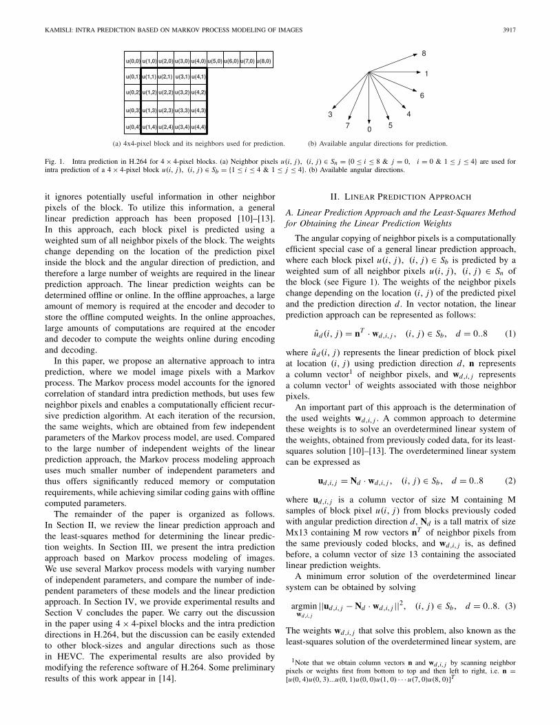
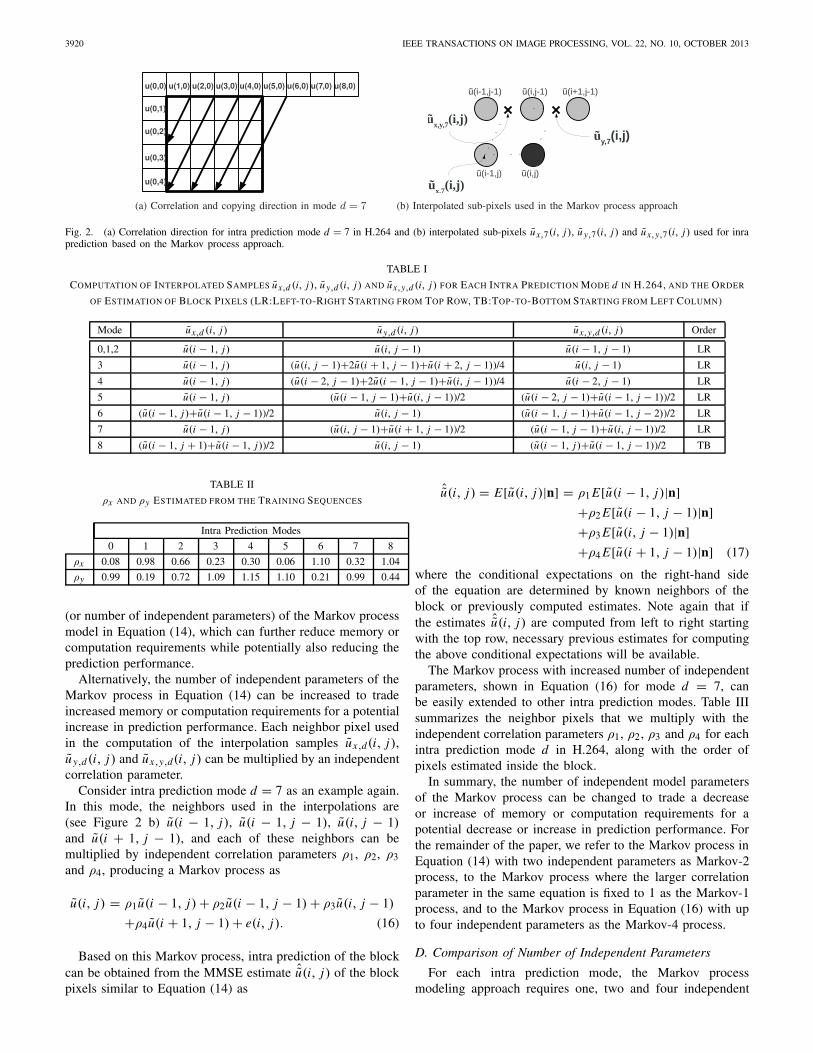
Consider intra prediction mode d = 7 as an example. In thismode, there is a high correlation along the angular directionshown in Figure 2 a), and H.264 or HEVC copy interpolationsof upper neighbor pixels along this direction inside the block.To account for the high-correlation along this direction in the

Markov process model, we choose u y,7(i, j) as the half-pixel((u(i, j −1)+ u(i +1, j −1))/2) between the upper and upper-right pixel of u(i, j) as shown in Figure 2 b), and to accountfor the potentially smaller correlation along a perpendiculardirection, we choose ux,7(i, j) as the left neighbor (u(i−1, j))of u(i, j). Finally, we choose ux,y,7(i, j) as the half-pixel((u(i − 1, j − 1) + u(i, j − 1))/2) between the upper-left andupper pixel of u(i, j) in order to complete a parallelogram.

To determine the intra prediction of the block, we obtainthe MMSE estimate û(i, j) from Equation (14) as

û(i, j) = E[u(i, j)|n]

= ρx E[ux,d(i, j)|n] + ρy E[u y,d(i, j)|n]

−ρxρy E[ux,y,d(i, j)|n], (15)

where E[u y,d(i, j)|n], E[ux,d(i, j)|n] and E[ux,y,d(i, j)|n]are given by corresponding interpolations of previously com-puted estimates or known neighbors. For prediction moded = 7,

E[u y,7(i, j)|n] = ( û(i, j − 1) + û(i + 1, j − 1))/2

E[ux,7(i, j)|n] = û(i − 1, j)

E[ux,y,7(i, j)|n] = ( û(i − 1, j − 1) + û(i, j − 1))/2.

Note that if the estimates û(i, j) are computed from left toright starting with the top row, necessary previous estimatesfor computing the above conditional expectations will beavailable.

The Markov process model in Equation (14) and the corre-sponding recursive estimation in Equation (15) can be usedto perform intra prediction along any angular direction byadjusting how the interpolated samples ux,d(i, j), u y,d(i, j)and ux,y,d(i, j) are computed. Table I shows how we obtainthese interpolated samples for each intra prediction directiond in H.264 along with the order of pixels estimated inside theblock.

Finally, as in Subsection III-A, we used a zero-meanprocess u(i, j) in this subsection, and to obtain the final intraprediction of the block, the means μu(i, j ) of block pixelsneed to be added to the recursively computed estimates as inEquation (13). In our experiments, we assume all pixels havethe same mean, which we obtain by averaging left and upperneighbor pixels of the block.

C. Markov Processes With Less and More IndependentParameters

The Markov process in Equation (14) has two independentparameters ρx and ρy , which can change depending on intraprediction mode. Table II shows ρx and ρy estimated froma set of training sequences for each intra prediction mode of4 × 4-pixel blocks. It can be seen from the table that, exceptfor intra prediction mode 2, either ρx or ρy is close to 1.This is expected since the parameter close to 1 representsthe correlation along the direction along which the neighborpixels are copied in standard intra prediction methods. Thusan alternative Markov process model can be one in which thelarger correlation parameter for each intra prediction mode isfixed to 1. This simplification reduces the degrees of freedom


Fig. 2. (a) Correlation direction for intra prediction mode d = 7 in H.264 and (b) interpolated sub-pixels ux,7(i, j), u y,7(i, j) and ux,y,7(i, j) used for inraprediction based on the Markov process approach.

TABLE I

COMPUTATION OF INTERPOLATED SAMPLES ux,d (i, j), u y,d (i, j) AND ux,y,d (i, j) FOR EACH INTRA PREDICTION MODE d IN H.264, AND THE ORDER

OF ESTIMATION OF BLOCK PIXELS (LR:LEFT-TO-RIGHT STARTING FROM TOP ROW, TB:TOP-TO-BOTTOM STARTING FROM LEFT COLUMN)

Mode ux,d (i, j) u y,d (i, j) ux,y,d (i, j) Order

0,1,2 u(i − 1, j) u(i, j − 1) u(i − 1, j − 1) LR

3 u(i − 1, j) (u(i, j − 1)+2u(i + 1, j − 1)+u(i + 2, j − 1))/4 u(i, j − 1) LR

4 u(i − 1, j) (u(i − 2, j − 1)+2u(i − 1, j − 1)+u(i, j − 1))/4 u(i − 2, j − 1) LR

5 u(i − 1, j) (u(i − 1, j − 1)+u(i, j − 1))/2 (u(i − 2, j − 1)+u(i − 1, j − 1))/2 LR

6 (u(i − 1, j)+u(i − 1, j − 1))/2 u(i, j − 1) (u(i − 1, j − 1)+u(i − 1, j − 2))/2 LR

7 u(i − 1, j) (u(i, j − 1)+u(i + 1, j − 1))/2 (u(i − 1, j − 1)+u(i, j − 1))/2 LR

8 (u(i − 1, j + 1)+u(i − 1, j))/2 u(i, j − 1) (u(i − 1, j)+u(i − 1, j − 1))/2 TB

TABLE II

ρx AND ρy ESTIMATED FROM THE TRAINING SEQUENCES

Intra Prediction Modes

0 1 2 3 4 5 6 7 8

ρx 0.08 0.98 0.66 0.23 0.30 0.06 1.10 0.32 1.04

ρy 0.99 0.19 0.72 1.09 1.15 1.10 0.21 0.99 0.44

(or number of independent parameters) of the Markov processmodel in Equation (14), which can further reduce memory orcomputation requirements while potentially also reducing theprediction performance.

Alternatively, the number of independent parameters of theMarkov process in Equation (14) can be increased to tradeincreased memory or computation requirements for a potentialincrease in prediction performance. Each neighbor pixel usedin the computation of the interpolation samples ux,d(i, j),u y,d(i, j) and ux,y,d(i, j) can be multiplied by an independentcorrelation parameter.

Consider intra prediction mode d = 7 as an example again.In this mode, the neighbors used in the interpolations are(see Figure 2 b) u(i − 1, j), u(i − 1, j − 1), u(i, j − 1)and u(i + 1, j − 1), and each of these neighbors can bemultiplied by independent correlation parameters ρ1, ρ2, ρ3and ρ4, producing a Markov process as

u(i, j) = ρ1u(i − 1, j) + ρ2u(i − 1, j − 1) + ρ3u(i, j − 1)

+ρ4u(i + 1, j − 1) + e(i, j). (16)

Based on this Markov process, intra prediction of the blockcan be obtained from the MMSE estimate û(i, j) of the blockpixels similar to Equation (14) as

û(i, j) = E[u(i, j)|n] = ρ1 E[u(i − 1, j)|n]

+ρ2 E[u(i − 1, j − 1)|n]

+ρ3 E[u(i, j − 1)|n]

+ρ4 E[u(i + 1, j − 1)|n] (17)

where the conditional expectations on the right-hand sideof the equation are determined by known neighbors of theblock or previously computed estimates. Note again that ifthe estimates û(i, j) are computed from left to right startingwith the top row, necessary previous estimates for computingthe above conditional expectations will be available.

The Markov process with increased number of independentparameters, shown in Equation (16) for mode d = 7, canbe easily extended to other intra prediction modes. Table IIIsummarizes the neighbor pixels that we multiply with theindependent correlation parameters ρ1, ρ2, ρ3 and ρ4 for eachintra prediction mode d in H.264, along with the order ofpixels estimated inside the block.

In summary, the number of independent model parametersof the Markov process can be changed to trade a decreaseor increase of memory or computation requirements for apotential decrease or increase in prediction performance. Forthe remainder of the paper, we refer to the Markov process inEquation (14) with two independent parameters as Markov-2process, to the Markov process where the larger correlationparameter in the same equation is fixed to 1 as the Markov-1process, and to the Markov process in Equation (16) with upto four independent parameters as the Markov-4 process.

D. Comparison of Number of Independent Parameters

For each intra prediction mode, the Markov processmodeling approach requires one, two and four independent


TABLE III

NEIGHBOR PIXELS THAT ARE MULTIPLIED WITH ρ1, ρ2 , ρ3 AND ρ4 FOR EACH INTRA PREDICTION MODE d IN H.264, AND THE ORDER OF

ESTIMATION OF BLOCK PIXELS (LR:LEFT-TO-RIGHT STARTING FROM TOP ROW, TB:TOP-TO-BOTTOM STARTING FROM LEFT COLUMN)

Mode ρ1 ρ2 ρ3 ρ4 Order

0,1,2 u(i − 1, j) u(i − 1, j − 1) u(i, j − 1) LR

3 u(i − 1, j) u(i, j − 1) u(i + 1, j − 1) u(i + 2, j − 1) LR

4 u(i − 1, j) u(i − 1, j − 1) u(i, j − 1) u(i − 2, j − 1) LR

5 u(i − 1, j) u(i − 1, j − 1) u(i, j − 1) u(i − 2, j − 1) LR

6 u(i − 1, j) u(i − 1, j − 1) u(i, j − 1) u(i − 1, j − 2) LR

7 u(i − 1, j) u(i − 1, j − 1) u(i, j − 1) u(i + 1, j − 1) LR

8 u(i, j − 1) u(i − 1, j − 1) u(i − 1, j) u(i − 1, j + 1) TB

TABLE IV

COMPARISON OF NUMBER OF INDEPENDENT PARAMETERS


3, 7, 8 0, 1, 2, 4, 5, 6 Total

Linear 4 × 4 blocks 16 × 13 = 208 16 × 9 = 14412816

Prediction 8×8 blocks 64 × 25 = 1600 64 × 17 = 1088


0, 1 2 3, 4, 5, 6, 7, 8 Total

Markov-14 × 4 blocks 1 2 1

208 × 8 blocks 1 2 1


368 × 8 blocks 2 2 2


668 × 8 blocks 3 3 4

parameters for Markov-1, Markov-2 and Markov-4 processes,respectively. The general linear prediction approach requiresmuch more independent weights (or parameters). Each usedneighbor pixel of the block requires linear prediction weights,which change depending on the predicted block pixel and onthe prediction mode. In our experiments, we use all shownneighbor pixels in Figure 1 (total of 13 for 4 × 4 blocks and25 for 8 × 8 blocks, i.e. 3B +1 neighbors where B is blocksize) for intra prediction modes 3,7 and 8, and only left, upper-left, and upper neighbors (total of 9 for 4×4 blocks and 17 for8 × 8 blocks, i.e. 2B +1 neighbors where B is block size) forremaining prediction modes. Table IV compares the numberof independent parameters required for each intra predictionmode in 4 × 4 and 8 × 8 blocks for linear prediction andMarkov process approaches.

The linear prediction weights and the Markov processparameters can be estimated offline or online. In case ofoffline determination of weights or parameters, the weightsor parameters can be either permanently saved in the encoderand decoder, or they can be determined by the encoder foreach sequence or frame and transmitted to the decoder withinthe bitstream. If the number of weights or parameters is small,they can be stored or transmitted more efficiently.

In case of online determination of weights or parameters,the weights or parameters are computed by the encoder anddecoder during encoding and decoding using previously codeddata available to both. If the number of weights or parametersis small, then the amount of computations for computing theweights or parameters will be less.

In summary, the Markov process approaches use signifi-cantly fewer independent parameters than the general linearprediction approach and this can have important benefits forthe implementation of these approaches.

IV. EXPERIMENTAL RESULTS

A. Results With Offline-Computed Global Linear PredictionWeights and Markov Process Parameters

We present experimental results to compare the standardintra prediction in H.2642 with the linear prediction approachand the Markov process modeling approaches both in terms ofachievable coding gains and the used number of independentparameters. In particular, we compare the following systems:

• H264: standard intra prediction in H.264/AVC• LP: linear prediction approach where, depending on pre-

diction mode, 2B +1 or 3B +1 (B is the block-size, seeTable IV) linear prediction weights are used for predictingeach block pixel in each intra prediction mode

• MRKV-1: intra prediction approach based on a Markov-1process model for image pixels



We have implemented these systems by modifying the KTAsoftware implementation of H.264 [17], and saved offlineestimated linear prediction weights or Markov process para-meters in the encoder and decoder of each system. Theweights for LP, and the parameters for MRKV-1, MRKV-2 andMRKV-4 were obtained offline from a training set whichconsists of 4 sequences listed in Table V. The weights andparameters estimated from the training set are then used forcoding sequences in the experiment set, which does not includeany of the training set sequences.

To estimate the weights and parameters from the trainingset, we intra-code every 10th frame of each sequence inthe training set using four different quantization parameters(QP = 37,32,27,22) and store the coded 4 × 4-pixel and8 ×8-pixel blocks (and their neighbor pixels) after classifying

2For the experiments in this paper we use the intra prediction framework inH.264, however, linear prediction and Markov process approaches can also beapplied to intra prediction in HEVC. How they interact with new coding toolsin HEVC and what coding gains they achieve in HEVC can be determined ifthey are tested within HEVC.


TABLE V

TRAINING SEQUENCES

Sequence Resolution

BQSquare-416 × 240-60 416 × 240

PartyScene-832 × 480-50 832 × 480

vidyo1-720p-60 1280 × 720

Kimono1-1920 × 1080-24 1920 × 1080

them according to their intra prediction modes. To estimatethe linear prediction weights for the LP system, we usean iterative approach, where each iteration consist of twosteps. In the first step, the weights for each class (i.e. intraprediction mode) are estimated using the least-squares solutionof overdetermined linear systems as shown in Equation (4).In the second step, data from all classes is re-classifiedby choosing the best intra prediction mode for each datausing the linear prediction weights estimated in the first step.We stop the iterations when the estimated weights don’tchange significantly, which takes about five iterations. Thisrecursive estimation approach provides more accurate weightsfor each intra prediction mode compared to estimating theweights directly from the initially classified data by theencoder.

Estimation of the Markov process parameters forMRKV-1, MRKV-2 and MRKV-4 systems from the same datais performed similarly, except the first step of the iterationsis different. Estimation of the Markov process parametersis a non-linear least-squares problem, and in the first stepwe use optimization tools in Matlab to estimate the Markovprocess parameters for each intra prediction mode from eachclass of data. In the second step, all data is re-classified bychoosing the best intra prediction mode for each block usingthe Markov process parameters estimated in the first step.We again stop after five iterations. Table VI lists the estimatedMarkov process parameters. The estimated weights used inLP are not shown since they require too much space. Theobtained weights and parameters are stored in the KTAsoftware with 10-bit integer accuracy.

It can be seen from Table VI that for MRKV-2, eitherρx or ρy is close to 1, except for intra prediction mode 2.The parameter close to 1 represents the correlation alongthe direction along which the neighbor pixels are copied instandard intra prediction methods. In MRKV-1, the largercorrelation parameter for each intra prediction mode is fixedto 1 to reduce the number of independent parameters. It canbe observed that the smaller correlation parameter of MRKV-2and MRKV-1 is always larger in 8 × 8-pixel blocks than in4 ×4-pixel blocks. For example, in intra prediction mode 1 ofMRKV-2, ρy is 0.19 for 4×4-pixel blocks and 0.50 for 8×8-pixel blocks. This is due to the fact that smoother regions offrames are typically more efficiently coded with larger block-sizes and less smoother regions with smaller block-sizes.

If MRKV-4 parameters are compared with MRKV-2 orMRKV-1 parameters for intra prediction mode 0, then it canbe observed that the ρ1 value is close to the ρx values,the ρ3 value is close to the ρy values, and the ρ2 value is

close to the negative product of ρx and ρy values. Similarobservations can be made also for modes 1 and 2, whichimply that the separable Markov process model holds wellfor these three modes and the additional independent para-meter of MRKV-4 is not leading to significant differencebetween the Markov process models of MRKV-2 (or MRKV-1) and MRKV-4. For other modes, however, the additionaldegrees of freedom provided by the increased number ofindependent parameters of MRKV-4 causes a more significantdifference between the Markov process models of MRKV-2(or MRKV-1) and MRKV-4.

Note that these weights and parameters are estimated fromencoding several sequences at diverse resolution, spatial char-acteristics, and picture qualities (or bitrates), and thereforethe estimated weights and parameters are intended to beglobal without any specific tuning to any resolution, spatialcharacteristics or picture quality.

Some important encoder configuration parameters are as fol-lows. We use high-complexity RD-optimized mode selection,CABAC for entropy coding, the in-loop deblocking filter, the8 × 8-block transforms, but turn off many of the new codingtools in KTA in order to avoid any complexity coming fromthe additional coding tools present in KTA. We code every10th frame of the test sequences used in our simulations andall of these frames are intra-coded. Coding is performed at fourdifferent quality levels using quantization parameters (QP) of37, 32, 27 and 22. In addition, we apply the linear predictionand the Markov process approaches only to the Y componentof coded frames, and intra prediction of chroma componentsis not changed.

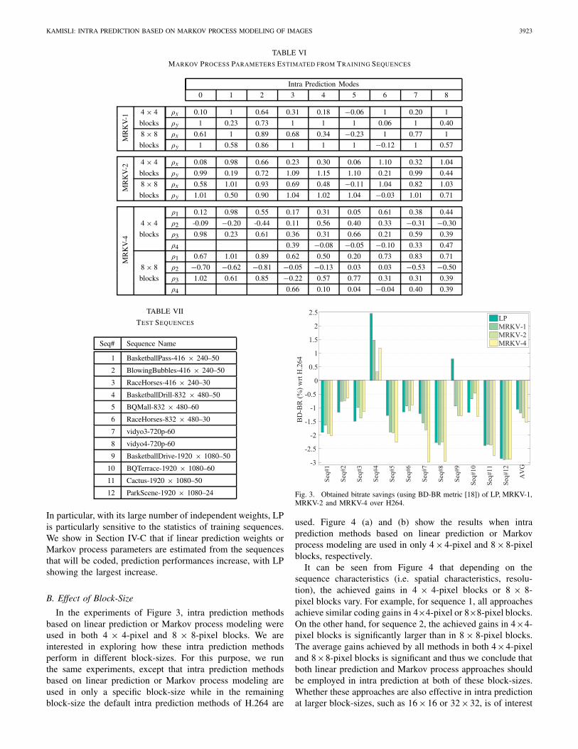
Our major goal in this section is to compare LP, MRKV-1,MRKV-2 and MRKV-4 in terms of the number of independentweights or parameters, and coding gains over H264. Thenumber of independent weights of LP and the number ofindependent parameters of Markov process approaches wereshown in Table IV, and Markov process approaches requirefar smaller number of independent parameters. To measure thecoding gains, we use the Bjontegaard-Delta bitrate (BD-BR)[18] metric using the PSNR of the Y component and the totalbitrate of all components. The BD-BR metric roughly gives theaverage percentage bitrate saving of one system with respect toanother system averaged over a range of picture qualities. Theused test sequences are listed in Table VII and the obtainedBD-BR metrics of LP, MRKV-1, MRKV-2 and MRKV-4 overH264 for each of the test sequences are shown in Figure 3.

It can be seen from Figure 3 that the average bitrate savingof LP, MRKV-1, MRKV-2 and MRKV-4 over H264 are 1.05%,1.19%, 1.37% and 1.54%, respectively. For some sequences,linear prediction and Markov process approaches performsimilar, and for some sequences their performances vary.Furthermore, for sequence 4, all approaches actually causea bitrate increase over H264. The linear prediction weightsin LP and the Markov process parameters in the Markovprocess approaches were estimated from 4 training sequences.If some of the test sequences, such as sequence 4 in particular,have significantly differing spatial statistics than the trainingsequences, intra prediction methods based on linear predic-tion and Markov process approaches may not perform well.


TABLE VI

MARKOV PROCESS PARAMETERS ESTIMATED FROM TRAINING SEQUENCES


0 1 2 3 4 5 6 7 8

MR

KV

-1

4 × 4 ρx 0.10 1 0.64 0.31 0.18 −0.06 1 0.20 1

blocks ρy 1 0.23 0.73 1 1 1 0.06 1 0.40

8 × 8 ρx 0.61 1 0.89 0.68 0.34 −0.23 1 0.77 1

blocks ρy 1 0.58 0.86 1 1 1 −0.12 1 0.57

MR

KV

-2

4 × 4 ρx 0.08 0.98 0.66 0.23 0.30 0.06 1.10 0.32 1.04

blocks ρy 0.99 0.19 0.72 1.09 1.15 1.10 0.21 0.99 0.44

8 × 8 ρx 0.58 1.01 0.93 0.69 0.48 −0.11 1.04 0.82 1.03

blocks ρy 1.01 0.50 0.90 1.04 1.02 1.04 −0.03 1.01 0.71

MR

KV

-4

ρ1 0.12 0.98 0.55 0.17 0.31 0.05 0.61 0.38 0.44

4 × 4 ρ2 -0.09 −0.20 -0.44 0.11 0.56 0.40 0.33 −0.31 −0.30

blocks ρ3 0.98 0.23 0.61 0.36 0.31 0.66 0.21 0.59 0.39

ρ4 0.39 −0.08 −0.05 −0.10 0.33 0.47

ρ1 0.67 1.01 0.89 0.62 0.50 0.20 0.73 0.83 0.71

8 × 8 ρ2 −0.70 −0.62 −0.81 −0.05 −0.13 0.03 0.03 −0.53 −0.50

blocks ρ3 1.02 0.61 0.85 −0.22 0.57 0.77 0.31 0.31 0.39

ρ4 0.66 0.10 0.04 −0.04 0.40 0.39

TABLE VII

TEST SEQUENCES

Seq# Sequence Name

1 BasketballPass-416 × 240–50

2 BlowingBubbles-416 × 240–50

3 RaceHorses-416 × 240–30

4 BasketballDrill-832 × 480–50

5 BQMall-832 × 480–60

6 RaceHorses-832 × 480–30

7 vidyo3-720p-60

8 vidyo4-720p-60

9 BasketballDrive-1920 × 1080–50

10 BQTerrace-1920 × 1080–60

11 Cactus-1920 × 1080–50

12 ParkScene-1920 × 1080–24

In particular, with its large number of independent weights, LPis particularly sensitive to the statistics of training sequences.We show in Section IV-C that if linear prediction weights orMarkov process parameters are estimated from the sequencesthat will be coded, prediction performances increase, with LPshowing the largest increase.

B. Effect of Block-Size

In the experiments of Figure 3, intra prediction methodsbased on linear prediction or Markov process modeling wereused in both 4 × 4-pixel and 8 × 8-pixel blocks. We areinterested in exploring how these intra prediction methodsperform in different block-sizes. For this purpose, we runthe same experiments, except that intra prediction methodsbased on linear prediction or Markov process modeling areused in only a specific block-size while in the remainingblock-size the default intra prediction methods of H.264 are

-3

-2.5

-2

-1.5

-1

-0.5

0

0.5

1

1.5

2

2.5

BD

-BR

(%) w

rt H

.264

Seq#

1

Seq#

2

Seq#

3

Seq#

4

Seq#

5

Seq#

6

Seq#

7

Seq#

8

Seq#

9

Seq#

10

Seq#

11

Seq#

12

AV

G

LPMRKV-1MRKV-2MRKV-4

Fig. 3. Obtained bitrate savings (using BD-BR metric [18]) of LP, MRKV-1,MRKV-2 and MRKV-4 over H264.

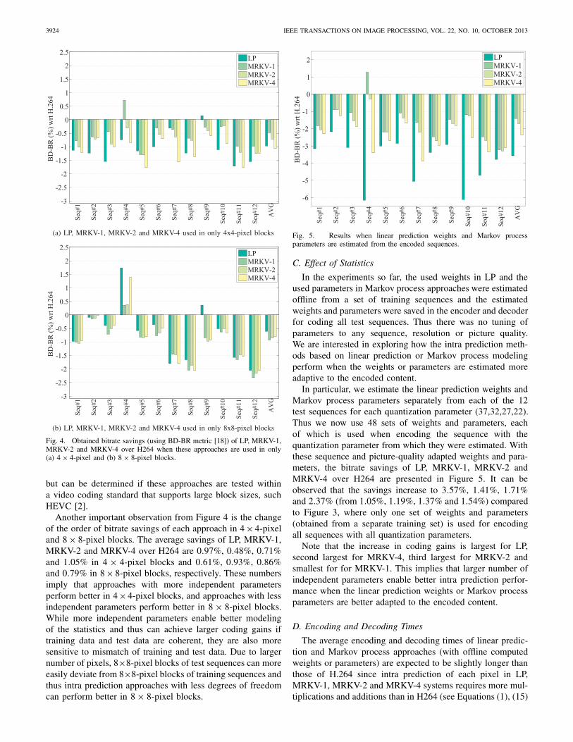
used. Figure 4 (a) and (b) show the results when intraprediction methods based on linear prediction or Markovprocess modeling are used in only 4 × 4-pixel and 8 × 8-pixelblocks, respectively.

It can be seen from Figure 4 that depending on thesequence characteristics (i.e. spatial characteristics, resolu-tion), the achieved gains in 4 × 4-pixel blocks or 8 × 8-pixel blocks vary. For example, for sequence 1, all approachesachieve similar coding gains in 4×4-pixel or 8×8-pixel blocks.On the other hand, for sequence 2, the achieved gains in 4×4-pixel blocks is significantly larger than in 8 × 8-pixel blocks.The average gains achieved by all methods in both 4×4-pixeland 8×8-pixel blocks is significant and thus we conclude thatboth linear prediction and Markov process approaches shouldbe employed in intra prediction at both of these block-sizes.Whether these approaches are also effective in intra predictionat larger block-sizes, such as 16 ×16 or 32 ×32, is of interest


Fig. 4. Obtained bitrate savings (using BD-BR metric [18]) of LP, MRKV-1,MRKV-2 and MRKV-4 over H264 when these approaches are used in only(a) 4 × 4-pixel and (b) 8 × 8-pixel blocks.

but can be determined if these approaches are tested withina video coding standard that supports large block sizes, suchHEVC [2].

Another important observation from Figure 4 is the changeof the order of bitrate savings of each approach in 4 × 4-pixeland 8 × 8-pixel blocks. The average savings of LP, MRKV-1,MRKV-2 and MRKV-4 over H264 are 0.97%, 0.48%, 0.71%and 1.05% in 4 × 4-pixel blocks and 0.61%, 0.93%, 0.86%and 0.79% in 8 × 8-pixel blocks, respectively. These numbersimply that approaches with more independent parametersperform better in 4 ×4-pixel blocks, and approaches with lessindependent parameters perform better in 8 × 8-pixel blocks.While more independent parameters enable better modelingof the statistics and thus can achieve larger coding gains iftraining data and test data are coherent, they are also moresensitive to mismatch of training and test data. Due to largernumber of pixels, 8×8-pixel blocks of test sequences can moreeasily deviate from 8×8-pixel blocks of training sequences andthus intra prediction approaches with less degrees of freedomcan perform better in 8 × 8-pixel blocks.

-6

-5

-4

-3

-2

-1

0

1

2

BD

-BR

(%) w

rt H

.264

Seq#

1

Seq#

2

Seq#

3

Seq#

4

Seq#

5

Seq#

6

Seq#

7

Seq#

8

Seq#

9

Seq#

10

Seq#

11

Seq#

12

AV

G

LPMRKV-1MRKV-2MRKV-4

Fig. 5. Results when linear prediction weights and Markov processparameters are estimated from the encoded sequences.

C. Effect of Statistics

In the experiments so far, the used weights in LP and theused parameters in Markov process approaches were estimatedoffline from a set of training sequences and the estimatedweights and parameters were saved in the encoder and decoderfor coding all test sequences. Thus there was no tuning ofparameters to any sequence, resolution or picture quality.We are interested in exploring how the intra prediction meth-ods based on linear prediction or Markov process modelingperform when the weights or parameters are estimated moreadaptive to the encoded content.

In particular, we estimate the linear prediction weights andMarkov process parameters separately from each of the 12test sequences for each quantization parameter (37,32,27,22).Thus we now use 48 sets of weights and parameters, eachof which is used when encoding the sequence with thequantization parameter from which they were estimated. Withthese sequence and picture-quality adapted weights and para-meters, the bitrate savings of LP, MRKV-1, MRKV-2 andMRKV-4 over H264 are presented in Figure 5. It can beobserved that the savings increase to 3.57%, 1.41%, 1.71%and 2.37% (from 1.05%, 1.19%, 1.37% and 1.54%) comparedto Figure 3, where only one set of weights and parameters(obtained from a separate training set) is used for encodingall sequences with all quantization parameters.

Note that the increase in coding gains is largest for LP,second largest for MRKV-4, third largest for MRKV-2 andsmallest for for MRKV-1. This implies that larger number ofindependent parameters enable better intra prediction perfor-mance when the linear prediction weights or Markov processparameters are better adapted to the encoded content.

D. Encoding and Decoding Times

The average encoding and decoding times of linear predic-tion and Markov process approaches (with offline computedweights or parameters) are expected to be slightly longer thanthose of H.264 since intra prediction of each pixel in LP,MRKV-1, MRKV-2 and MRKV-4 systems requires more mul-tiplications and additions than in H264 (see Equations (1), (15)


TABLE VIII

COMPARISON OF AVERAGE ENCODING AND DECODING TIMES

Method H264 LP MRKV-1 MRKV-2 MRKV-4

Encoder 100.0% 121.0% 108.8% 109.3% 108.4%Decoder 100.0% 111.6% 106.2% 106.8% 105.7%

and (17)). We averaged the increase in encoding and decodingtimes of LP, MRKV-1, MRKV-2 and MRKV-4 systems withrespect to H264 for all test sequences at quantization parameter32 and the results are shown in Table VIII. It can be seen inthe table that the increase of encoding and decoding timesis larger in LP than in Markov process approaches since LPrequires more multiplications and additions.

Note that since the weights or parameters are computedoffline, the increase in encoding and decoding times is smalland comes only from the increase in the number of multi-plications and additions of the prediction. If, however, theweights or parameters are computed online, adapted to eachblock during encoding and decoding, additional computationsfor estimating these weights or parameters are required andthe encoding and decoding times are likely to increase muchmore significantly [10], [12], [13]. However, while the linearprediction approach requires the online estimation of manyweights, the Markov process approaches require the onlineestimation of much fewer parameters (see Table IV), and thusthe increase of encoding and decoding times of the Markovprocess approaches is expected to be smaller than that of linearprediction approaches. We intend to explore these aspects inour future research.

V. CONCLUSION

In standard intra prediction methods, neighbor pixels ofthe block are copied along an angular direction inside theblock and thus each block pixel is predicted from only oneor few directionally aligned neighbor pixels of the block. Thisapproach is computationally efficient but it ignores poten-tially useful correlation of other neighbor pixels. One way toutilize this correlation is a general linear prediction approach,where each block pixel is predicted using a weighted sumof all neighbor pixels of the block. However, general linearprediction requires a large number of weights, which increasesmemory requirements if the weights are stored or computationrequirements if the weights are computed online.

This paper proposed an alternative approach to intra predic-tion, where image pixels are modeled with Markov processes.The Markov processes account for the ignored correlation (instandard intra prediction methods) using few neighbor pixelsand enable a computationally efficient recursive predictionalgorithm. Compared to the large number of independentweights of the general linear prediction approach, the Markovprocess modeling approach uses much smaller number ofindependent parameters and thus offers reduced memory orcomputation requirements. In the experiments with offline-computed linear prediction weights and Markov process para-meters, both approaches achieved similar coding gains despitethe significant difference in the stored number of weights andparameters.

Future research directions include exploration of codinggain-complexity trade-off when Markov process parametersare estimated online during encoding and decoding. Exploringuse of adaptive transforms based on the estimated processparameters is also of interest.

REFERENCES

[1] T. Wiegand, G. Sullivan, G. Bjontegaard, and A. Luthra, “Overview ofthe H.264/AVC video coding standard,” IEEE Trans. Circuits Syst. VideoTechnol., vol. 13, no. 7, pp. 560–576, Jul. 2003.

[2] G. Sullivan, J. Ohm, W.-J. Han, T. Wiegand, and T. Wiegand, “Overviewof the high efficiency video coding (HEVC) standard,” IEEE Trans.Circuits Syst. Video Technol., vol. 22, no. 12, pp. 1649–1668, Dec. 2012.

[3] J. Lainema, F. Bossen, W.-J. Han, J. Min, and K. Ugur, “Intra coding ofthe HEVC standard,” IEEE Trans. Circuits Syst. Video Technol., vol. 22,no. 12, pp. 1792–1801, Dec. 2012.

[4] S. Yu and C. Chrysafis, “New intra pre-diction using intra-macroblockmotion compensation,” in Proc. 3rd Meeting, Joint Video Team, 2002,pp. 1–6.

[5] T. K. Tan, C. S. Boon, and Y. Suzuki, “Intra prediction by tem-plate matching,” in Proc. IEEE Int. Conf. Image Process., Oct. 2006,pp. 1693–1696.

[6] J. Balle and M. Wien, “Extended texture prediction for H.264/AVC intracoding,” in Proc. IEEE Int. Conf. Image Process., vol. 6. Oct. 2007,pp. 93–96.

[7] T. Shiodera, A. Tanizawa, and T. Chujoh, “Bidirectional intra predic-tion,” in Proc. VCEG, Meeting Marrakech, Morocco Conf., Jan. 2007,pp. 1–10.

[8] J. Lainema and K. Ugur, “Angular intra prediction in high efficiencyvideo coding (HEVC),” in Proc. IEEE 13th Int. Workshop MultimediaSignal Process., Oct. 2011, pp. 1–5.

[9] S. Yu, Y. Gao, J. Chen, and J. Zhou, “Distance-based weighted predictionfor H.264 intra coding,” in Proc. Int. Conf. Audio, Lang. Image Process.,Jul. 2008, pp. 1477–1480.

[10] L. Liu, Y. Liu, and E. Delp, “Enhanced intra prediction using context-adaptive linear prediction,” in Proc. Picture Coding Symp., 2007,pp. 1–4.

[11] L. Zhang, X. Zhao, S. Ma, Q. Wang, and W. Gao, “Novel intra predictionvia position-dependent filtering,” J. Vis. Commun. Image Represent.,vol. 22, no. 8, pp. 687–696, Nov. 2011.

[12] J. Chen and W.-J. Han, “Adaptive linear prediction for block-based lossyimage coding,” in Proc. IEEE Int. Conf. Image Process., Nov. 2009,pp. 2833–2836.

[13] D. Garcia and R. de Queiroz, “Least-squares directional intra predictionin H.264/AVC,” IEEE Signal Process. Lett., vol. 17, no. 10, pp. 831–834,Oct. 2010.

[14] F. Kamisli, “Intra prediction based on markov process modeling ofimages,” in Proc. IEEE ICIP, Feb. 2013, pp. 1–3.

[15] J. Han, A. Saxena, V. Melkote, and K. Rose, “Jointly optimizedspatial prediction and block transform for video and image cod-ing,” IEEE Trans. Image Process., vol. 21, no. 4, pp. 1874–1884,Apr. 2012.

[16] C. Yeo, Y. H. Tan, Z. Li, and S. Rahardja, “Mode-dependent transformsfor coding directional intra prediction residuals,” IEEE Trans. CircuitsSyst. Video Technol., vol. 22, no. 4, pp. 545–554, Apr. 2012.

[17] (2005, Jan.). Key Technical Areas (KTA) [Online]. Available:http://iphome.hhi.de/suehring/tml/download/KTA/

[18] G. Bjontegaard, “Calculation of average PSNR differences betweenRD-curves,” in Proc. VCEG Meeting, Apr. 2001, pp. 1–9.

Fatih Kamisli (S’09–M’11) received the B.S. degreefrom the Middle East Technical University, Ankara,Turkey, in 2003, and the M.S. and Ph.D. degreesin electrical engineering and computer science fromthe Massachusetts Institute of Technology in 2006and 2010, respectively.

He is an Assistant Professor with the Electrical andElectronics Engineering Department, Middle EastTechnical University. His current research interestsinclude image and video processing.

Documents

Intra Prediction Based on Markov Process Modeling of Images