Embed Size (px)
Citation preview

Estimating Financial Volatility with High-Frequency Returns
Long H. Vo ∗
Abstract: The primary value of a time series model lies in its ability to provide reliableapproximations of the modelled variable, both in-sample (where data are used to estimate modelparameters) and out-of-sample (where the model is updated with new information and producesforecasts). In this paper, an overview of the various models in the GARCH family is followed bytheir application in estimating the daily volatility of Citigroup Inc., a major player in the US sub-prime mortgage crisis. Fitting these estimates to the ex-post realized volatility measure constructedfrom high-frequency returns provides superior goodness-of-fit than fitting them to the conventionalabsolute returns measure. This suggests that when modelling latent financial volatility, informationrevealed by high-frequency data can greatly enhance GARCH estimates’ performance.
Keywords: Realized volatility, GARCH models, frequency domain analysis, high-frequency
data.
Introduction
Poon and Granger (2003) emphasis the role of volatility in modern finance literature. Theimportance of volatility is apparent in a large variety of disciplines, of which the follow-ing are but a few: derivative pricing (e.g. option pricing depends heavily on underlyingstock’s volatility), risk management (volatility forecasting has become crucial to determin-ing Value-at-risk especially after the global implementation of the first Basel Accord in1988) and policy making (which relies on estimates of financial vulnerability via proxies ofrisk such as volatility).
Understanding the nature of volatility is therefore becoming ever more crucial in finan-cial modelling. Taylor (2005) proposed one of the most popular definitions of this variable:it is defined by standard deviation of a historical set of returns {rt|t = 1, . . . , T} whose
mean is r = µ =1
T
T∑t=1
rt. The formula is thus:
σ =
√√√√ 1
T − 1
T∑t=1
(rt − r)2 (1)
∗Faculty of Finance, Banking and Business Management, Quy Nhon University, Binh Dinh, Vietnam.E-mail: [email protected]. This paper is based partly of my dissertation at Victoria University ofWellington, New Zealand. I thank the constructive comments of Leigh Roberts, Graeme Guthrie and TobyDaglish. For providing the tick-data I thank the Securities Industry Research Centre of Asia-Pacific (SIRCA).Financial support from the New Zealand-ASEAN scholarship scheme is gratefully acknowledged. All errorsremain with the author.
84
Journal of Finance & Economics ResearchVol. 2(2): 84-114, 2017DOI: 10.20547/jfer1702201

Journal of Finance & Economics Research
Simply put, the volatility of an asset is the standard deviation of the returns on thatasset away from its equilibrium (long-run mean) over a period of time (Hull, 2006). In thefinance literature, volatility is commonly measured by the absolute value of the returns.Though statistically improper, absolute value provides the best estimate of the standarddeviation of a single return at a single period (Taylor, 2005; Boubaker & Raza, 2017).
As volatility captures the variability in asset prices, it is generally taken as a proxy forrisk. Poon and Granger (2003) examine volatility via the continuous time martingale thatgenerates instantaneous returns:
d(lnpt) = σt dWp,t (2)
where pt is the stock price and dWp,t denotes a standard Wiener process. In thiscontext, volatility can be thought of as a ‘scale’ parameter which adjusts the size of thevariation associated with a stochastic Wiener process. Then, the conditional variance
of this return over the period [t, t+ 1] is called the ‘integrated volatility’:
∫ 1
0
σ2t+τdτ .
Fundamental derivatives pricing theories were built upon this quantity under stochasticvolatility (See for example Melino (1991), Hull and White (1996) and Hull (2006)). Ingeneral, σt is unobservable. However, if we can obtain a sufficiently large number ofcontinuously compounded returns over one time unit, the sum of the squared value ofthese returns shall provide us with a consistent estimate of the integrated volatility. Thisestimate is known as ‘realized volatility’.
Poon and Granger (2003) show that the accuracy of the realized estimate increases withthe number of returns (or the sampling rate) computed at higher frequency. Proof of thisproposition can also be found in (Barndorff-Nielsen & Shephard, 2002; Chen, 2014). Thismeans that given high-frequency data availability, the latent volatility process is plausiblyobservable. Beside being an ‘error-free’ volatility estimator, realized volatility is relativelysimple to compute. A number of studies illustrated the importance of volatility measuresconstructed from returns recorded at high frequencies (See e.g. (Andersen & Bollerslev,1998; Andersen, Bollerslev, Diebold, & Labys, 1999) among others).
As the name suggested, high-frequency financial data are recorded much more fre-quently than the ‘standard’ data (e.g. daily data). Traditionally, the data used in pub-lished studies of financial time series analysis are both low-frequency and regularly spaced,while availability of high-frequency data has not resulted in a comprehensive literatureuntil recently. This is due to the fact that low sampling rate of data can help reducethe costs of collection and storage significantly, and the equally spaced data points madeit simpler to developed statistical inferences, though with limited confidence (Dacorogna,Gencay, Muller, Olsen, & Pictet, 2001). Incidentally, most high-frequency data are basedon information arriving randomly and directly from markets, such as quoted prices fromintraday transactions. This feature makes it very difficult to study these data using meth-ods that are designed for analysing equally spaced time series. On the other hand, onecritical advantage introduced by huge influxes of high-frequency information, in terms ofgoodness-of-fit tests, is we can readily reduce the number of testing specifications 1. This
1Hereafter high-frequency refers to any frequency higher than daily, i.e. intraday data.
85

Journal of Finance & Economics Research
is because statistical uncertainty decreases as the frequency of observations rises (Muller etal., 1995). In this paper, using returns computed from a unique set of high-frequency data,we shall illustrate the distinct advantage of these data in obtaining more precise estimatesof realized volatility.
The rest of the paper is organized as follows: Section 2 discusses the importance of high-frequency data in greater details and introduce several ‘stylized facts’ of high-frequencyreturns. Section 3 introduces some popular models in the Generalized AutoregressiveConditional Heteroskedasticity (GARCH) family. Section 4 examines and compare thestylized facts of financial returns computed from both daily and intradaily data. Section 5fits the GARCH model to our daily data and discuss the goodness-of-fit in-sample.
Section 6 demonstrates the improved performance of GARCH out-of-sample when weuse a realized volatility measure constructed from high-frequency data. In addition, newevidence from multi-scale analysis suggests our wavelet decomposition may provide a betterway of approximating the true volatility factor. Section 7 gives some concluding comments.
The Importance of High-frequency Data
Improvement on Volatility Estimates
Merton (1980) argued that high frequency sampling significantly improves the accuracy ofthe time-varying variance estimate of the price process, although this paper was restrictedto only monthly and daily data. In line with this argument, Martens (2001) explicitly mod-elled intraday volatility and concluded that the forecast of daily volatility using intradayreturns is superior to that of the traditional approach using daily returns. In addition, themajor contribution of the seminal paper by Nelson (1992) is that the accuracy of volatilityestimates can be greatly improved with sufficiently frequently sampled data, even withvery short calendar time spans. The evidence of similar insights is intuitively provided byAndersen and Bollerslev (1998), in which the authors give a clear explanation of the poorout-of-sample predictive power of the GARCH model family despite adequate in-sample fit.The problem, as they pointed out, is not from the well-specified models themselves, but theex-post volatility measurements. The conventionally used squared return innovations wasproved to be a very noisy, albeit unbiased, proxy for the latent volatility. This motivatesthese authors to introduce the so-called realized volatility which is defied as cumulativesquared intraday returns. They also noted that “this measure converges to genuine mea-surement of latent volatility factor” (effectively making volatility ‘observable’ given thatthe sampling frequency increases indefinitely. Additionally, previous studies came to thecommon conclusion that due to specific market characteristics, realized volatility measuredfrom returns computed at very small intervals (in particular less than five minutes) is morelikely to be contaminated by micro structure effects (most notably non-synchronous tradingand bid-ask bounce) (Poon & Granger, 2003). Evidently, using high-frequency data enablesus to compute superior estimates of lower-frequency volatilities. Andersen, Bollerslev, andCai (2000) examined the intraday volatility of Japanese stock market, and documented adistinctive U-shaped pattern closely following intraday trading periods, in which volatilitytends to be high in the opening and closing of market while decreasing throughout the day.
86
Journal of Finance & Economics Research
Another important aspect of intraday data is that they can be used to investigate thedifference in the dependence structure of volatility at different frequencies. In some cases,such as in a GARCH (1,1) model, inter-temporal aggregation is theoretically proved to beable to preserve volatility structure (See Drost and Nijman (1993)). However, empiricalevidence generally suggests otherwise: volatility modelled at high frequencies exhibits muchstronger persistence than at low frequencies Diebold (1988). This notion is, in principle,in line with Nelson (1991) and is supported by Glosten, Jagannathan, and Runkle (1993),whose main finding is that persistence in volatility seems to diminish significantly whenmoving from daily to monthly data. Likewise, Andersen and Bollerslev (1997) argued thatthe long-memory behaviour observed in daily data also characterizes the volatility processat high frequencies, after filtering out all intraday dependencies.
With regard to the examination of high-frequency stylized facts, Andersen and Boller-slev (1997) noted the sharp contrast between the highly dependent dynamic in daily volatil-ity to a less profound long-term dependence among intraday volatility. According to theseauthors, the seemingly contradictory evidence of volatility persistence in daily and in-tradaily data is attributable to the fact that intraday volatility can be regarded as “[The]aggregation of numerous constituent component processes; some with very short-run decayrates [which dominate in intraday returns] and others possessing much longer-run depen-dencies”. In turn, the multiple volatility components at the intradaily frequencies are aresult of numerous heterogeneous information arrival processes. From a different angle,Jensen and Whitcher (2000) capture the presence of both short and long-memory (as aresult of unexpected as well as anticipated news) with a non-stationary, but locally station-ary, stochastic volatility estimator. Their primary finding is a time-varying long-memoryparameter which exhibits an intradaily pattern: being highest and lowest in accordancewith the opening and closing of foreign exchanges. These authors open up the debate ofwhether this strong time-of-the-day effect is caused by public macroeconomic news an-nounced at the beginning of some markets, or the capitalization of informed traders atthe end of other markets. In any case, the link between volatility dependence structureand the pattern in which new information arrives is central in understanding market op-erating dynamics. Furthermore, the evidence that long-memory parameter peaks at theclose of most active trading exchanges documented by Jensen and Whitcher (2000) andheterogeneous volatility structures captured by Andersen and Bollerslev (1997) both pointto the association between the persistence of volatility and less active, less volatile tradingsessions.
The Stylized Facts of High-frequency Financial Returns
The most notable fact of financial returns is perhaps the Non-normal (or Non-Gaussianity)or the heavy tailed distribution. Earlier empirical analyses dated as far back as the 1970shad repeatedly placed much emphasis on documenting related visual features and numerousimplications of returns’ distribution such as its approximate asymmetry, the heavy tailsand its high peak (see, for example, (Mandelbrot, 1963; Fama, 1965).
Dacorogna et al. (2001) and Taylor (2005) documented and summarized several stylizedfacts of volatility for both low-frequency and high-frequency returns. Because there are
87

Journal of Finance & Economics Research
variations in their orders and wordings, we believe it is helpful to list the propositionsin group of ‘traditional’ categories, namely: facts about distributions, autocorrelations,seasonality and scaling properties:
• The middle price is subject to microstructure effects at the highest frequency
• Intraday returns exhibit distribution with heavy tails, with increasing kurtosis pro-portional to increase in observation frequency
• Intraday returns from traded assets are almost uncorrelated, a part from a significantfirst-order correlation
• There exists seasonal volatility clusters distinctive to different days of the week
• There exists short bursts of volatility following arrival of major macroeconomic news
Our main interest is placed on the long-memory property exhibited by measures ofdaily and intradaily volatility. Poon and Granger (2003) assert that slow decay autocorre-lation of variances is a very well-established stylized fact throughout the literature (refer toGranger, Spear, and Ding (2000) for further reviews). According to Andersen and Boller-slev (1997), long-term dependency is an inherent characteristic of the underlying volatilitygenerating process. These authors also attribute the inconsistent conclusions about thelevel of volatility dependence to the fact that volatility process is actually a sum of multi-ple components. Volatility estimates are therefore affected by either short-run components(when using high-frequency data) or long-run ones (when using daily data). However,with appropriate restrictions imposed, the aggregated volatility process always exhibitslong memory. Christensen and Nielsen (2007) and Fleming and Kirby (2011) as well asmany academics having experience in the field agreed upon the feasibility of describing re-alized volatility with a fractionally integrated process where the long memory parameter dis within the range of 0.3 - 0.5. However, they also documented short-lived modest impactsof volatility changes on stock prices. In any case, volatility long-run dependence structurepossesses a complex nature.
An important question is that what makes the existence of long range dependencecrucial to studies of financial time series? One problem with the classical asset pricingtheories is pointed out by Lo (1991): whenever such dependence structure exists amongfinancial returns, the traditional statistical inference for tests of the capital asset pricingmodel and the arbitrage pricing theory, both of which rely on a martingale returns process,is no longer valid. Furthermore, the larger the long-memory effect, the greater the impactof shocks on future volatility. In practice, however, financial returns are almost alwaysobserved to be uncorrelated and thus exhibit very little long-run dependence.
Modelling Volatility with the GARCH Family
The foundation of a model that could effectively capture all the stylized facts of returnshas attracted enormous attention over time. In the time domain, there are two classes
88

Journal of Finance & Economics Research
of volatility models that enjoy vast popularity among academics, namely: the GARCHfamily models and the stochastic volatility models. While the former studies volatility as afunction of observables, the latter incorporates not only observables, but also unobservablevolatility components (See (Taylor, 2005) for a review of the topic). For our purposes,it is sufficient to study the first branch, which originates from the introduction of theAutoregressive Conditional Heteroskedastic (ARCH) model first proposed in the seminalpaper of (Engle, 1982). This model is designed to capture the time-varying nature ofconditional volatility given the historic information of returns. It is important to notethat stylized facts of volatility serve as theoretical motivations of specific extensions ofthe ARCH model. The paper by Engle and Patton (2001) reviews major stylized facts ofvolatility that should be incorporated in a good model. Specifically, these facts include:(i) volatility clusters, (ii) persistence, (iii) mean reversion and (iv) asymmetric impacts ofinnovations. Unable to cover the enormous body of research on this model family, ourpaper only investigates the frameworks most directly designed to incorporate these fourstylized facts. Next we shall discuss the salient specifications and their relevance to ourresearch in more detail.
Following the traditional approach we define the one-period continuously compounde-dreturns as the first order difference of the natural logarithm of a discrete price sequence.As Taylor (2005) argued, the number of dividend payment days is very small compared tothe sample of trading days and thus dividend can be ignored in this setting:
rt = ln(pt)− ln(pt−1) = ∆ln(pt) (3)
Assuming that asset returns are generated by the following process 2:
rt = µt + σtzt where zt ∼ i.i.d N(0,1) (4)
in which µt|t−1 = Et−1[rt] and σt|t−1 = Et−1[(rt − µt)2] are the process’ conditional meanand variance respectively, given the information set at time t−1 (which is the set of returnsup to t− 1, inclusive).
We also specify the ‘residual returns’ as ut = rt − µt = σtzt. Note that the conditionalmean µt tends to be modelled as an ARMA process in some contexts in order to free theresiduals of serial correlations. Nevertheless this variable is usually set to zero or constant3, as over the long term, in a large sample the average returns tend to be insignificant(Taylor, 2005) 4. The (population) unconditional mean and variance can be defined as:
µ = E[rt] and σ2 = E[(rt − µ)2] (5)
2This is the standard specification of all ARCH-type models examined in this paper. Therefore weimplicitly assume it in most of the later discussions.
3In general there are three specifications for conditional mean µt: we can treat it as zero, a constant, oradding an ARCH term determinant (meaning the expected value of returns also depends on past evaluationof volatility). The last type is commonly referred to as the ARCH-in-mean or ARCH-M model. Thedifference only results in different forecast of returns while not affecting our main interest - the volatilityestimates - in any significant way.
4Which is why the residual returns (or ‘de-meaned’ returns) and original returns series have similarproperties and the two are interchangeably used in different GARCH specifications. From our perspectivethese processes also have the same conditional variance.
89
Journal of Finance & Economics Research
As the name suggests, ARCH models conditional volatility auto-regressively, meaning fu-ture volatility is specified to be linearly dependent on immediate previous squared residualreturns. In other words, large/small deviations from mean return is followed by high/lowsubsequent variances. This allows us to effectively capture volatility clustering feature andis one of the reasons for the original success of the ARCH-type model:
σ2t = ω + α(u2
t−1) (6)
with ω > 0, α > 0. This is the simplest form of ARCH: the ARCH(1) model. When weincrease the number of autoregressive terms to p, we have its extended form: the ARCH(p)model 5:
σ2t = ω +
p∑i=1
αiu2t−i (7)
As Campbell, Lo, and MacKinlay (1997) pointed out, setting volatility to be time-varyingallows us to capture basic stylized facts of financial returns, most notably the propertythat returns’ distribution is heavy tailed with excess kurtosis.
In this case the returns process is stationary only if
p∑i=1
αi < 1 (with αi > 0∀i) so that
it has a finite long term unconditional variance, which can be computed as σ2 = Var(ut) =ω
1−∑pi=1 αi
. Also, the ARCH process is then mean-reverting.
The GARCH (1,1)
Despite its inherent ability to capture volatility clustering, ARCH model fails to account forvolatility persistence, as the clusters are short-lived without accounting for extra laggedut terms. Bollerslev (1986) augmented this model by adding a lagged term of condi-tional volatility, forming the Generalized Autoregressive Conditional Heteroskedasticity(GARCH) (1,1) model 6:
σ2t = ω + α(u2
t−1) + βσ2t−1 (8)
where ω > 0, α > 0, β > 0 and α + β < 1. It can be shown that the GARCH (1,1)is analogous to an ARCH(∞) 7. The GARCH (1,1) inherits its predecessor’s ability tocapture the excess kurtosis of returns’ distribution. Furthermore, the most important
5p is also known as the lag parameter in this context.6Also, ARCH model is analogous to an AR model on squared residuals, whilst GARCH can be thought
of as an ARMA model on squared residuals.7By recursively replacing the past volatility terms with their GARCH forms we can write the GARCH
model as:
σ2t = ω + αu2t−1 + βσ2
t−1
= ω + αu2t−1 + β(ω + αu2t−2 + βσ2t−2) = · · · =
ω
1− β+ α/β
∞∑j=1
βju2t−j
So that it becomes an ARCH(∞) model.
90

Journal of Finance & Economics Research
application of this model is its ability to forecast future volatility. We have the l-aheadvolatility forecast specified via:
σ2t+l = σ2 + (α+ β)l(σ2
t − σ2) (9)
Here the term (α + β) is known as ‘persistence parameter’ as it determines the rate atwhich the variance forecast converges to the long-run unconditional variance σ2 = E[u2
t ] =ω
1− (α+ β)when the forecast horizon tends to infinity (l→∞). To describe this particular
implication of GARCH, Engle (2001) stated that “the GARCH models are mean revertingand conditionally heteroskedastic, but have a constant unconditional variance”(p.160). Thisis an important complement of GARCH to ARCH. A related quantity specifying the degreeof volatility persistence is the ‘half-life’, denoted as k. It is the time needed for the varianceto move halfway towards its unconditional level. Generally we have (α + β)k = 0.5 ork = ln(0.5)/ln(α+ β). For the GARCH model to be stationary we must have (α+ β) < 1.We can write the generalized form of this model as:
σ2t = ω +
p∑i=1
αiu2t−i +
q∑j=1
βjσ2t−j (10)
For the sake of tractability we only focus on the simple GARCH (1,1) as well as its relatedmodels with the same ARMA order from here on. Many researchers strongly suggest thecomparability of such simple models to the ones incorporating higher order ARMA terms.Furthermore, it is widely documented that GARCH (1,1) generally equals or rivals other,more complex models in the same family, especially in terms of out-of-sample forecastperformance (See Hansen and Lunde (2005)).
Data
Our main focus in this section would be to provide a preliminary investigation on Citi-group’s stock prices and returns over the last 30 years or so. Here, we explore some pre-liminary analyses of daily returns and volatility, with emphases on the so-called ‘stylizedfacts’, specifically the heavy-tailed distribution and the autocorrelation structure. Detaileddescription of this company and its role in the Global financial crisis is provided in Ap-pendix A. This is followed by description of our transformation of daily prices into returnsin Appendix B.
Stylized Facts of Returns
We collect daily closing prices of Citigroup between 03 Jan 1977 and 31 Jul 2013 fromhttp://finance.yahoo.com. To get a first impression of the data, following the work ofCheng, Roberts, and Wu (2013), we simply concatenate the price series over the weekendsand holidays. This means we effectively ignore any missing data in our sample of 30years daily data, obtaining a total of 9228 daily returns. Figure 1 shows the time series
91
Journal of Finance & Economics Research
of Citigroup’s closing price and closing price adjusted for stock splits and dividend, aswell as their corresponding returns series (computed by concatenating method). Somemost notable features of these series are: (i) the price spikes just before 1998 (the yearof the merger between Citicorp and Travelers Group) and exhibits some volatility beforecontinuing to grow; (ii) there are two other major falls of the stock, corresponding to the2000s Internet bubble bust and Enron scandal (2002) as well as the recent GFC (aboutright after the rescue package the firm received); (iii) the huge downward trends lead to themost volatile period in returns from 2008 to 2010. In addition, when comparing the closingand adjusted closing price series, a very strong impression is the extremely different scaleson the two graphs. In subsequent analyses we shall focus on the ‘adjusted’ returns timeseries, in which the definition of one-period continuously compounded returns is establishedas in Section 3, where Pt is the adjusted closing price at time t, i.e. rt = lnPt − lnPt−1.
Asymmetric Impact of Returns on Volatility
A stylized fact that is widely documented in quantitative finance researches is the neg-ative correlation between stock returns and their volatility. This phenomenon is largelyattributed to the changes in leverage ratio corresponding to changes in stock prices. Inparticular, a fall in stock price generally has a much larger impact on volatility than arise of the same magnitude, since it causes the debt-to-equity ratio to rise, thus provokingequity investors’ concern about their claim in the firm. We can illustrate this feature byplotting the stock prices against corresponding absolute returns (as a conventional proxyfor volatility):
For the period from 1977 to 2008 the increase in share price results in relatively lowlevel of volatility that is distinct from that of the period from 2008 to 2010. From Figure2 we can see clearly the inverse direction/sign exhibited by stock returns and volatility:whenever prices go down, volatility goes up and vice versa. Furthermore, the impacts ofpositive and negative price changes on volatility are dramatically different: a steep risefrom 1995 to mid 2007 (indicated by the green trend line) results in a change of volatilitythat has roughly the same magnitude as the change corresponding to the period from mid2007 to 2009 (indicated by the red trend line). In other words, the strong fall during thethree years of GFC undid the gain built up in previous 12 years and was undoubtedlyrelated to one of the most volatile, unprecedented periods in the history of the financeworld. Aside from this obvious feature, the asymmetric relation between price changes andvolatility is repeated throughout Citigroup’s timeline.
This relationship was explicitly studied via the specification of asymmetric GARCHmodels earlier. It will be further elaborated at different time horizons in later sections viathe investigation of the leverage effect hypothesis.
On the other hand, looking at Figure 2 one can argue that the relationship betweenthe direction of price movement and the magnitude of volatility can be somewhat expectedand the above argument about impact of the sign is not necessarily applicable. The reasonis that if we consider volatility to be proportional to the absolute value of the quantity∆P
P(where P is the price) then surely the volatility of period 2007-2009 is much greater
than that of period 1995-2007. This is simply because this quantity is also proportional
92
Journal of Finance & Economics Research
to the slope of the trend lines associated with these periods. The longer the period, thesmaller the slope (in terms of absolute value) and vice versa.
Figure 1Time series plot of Citigroup daily data. From top to bottom: close price, returns (close-to-close),adjusted close price, returns (adjusted close-to-adjusted close). Data range from 03 Jan 1977 to31 Jul 2013.
This counter argument implies that what really affects volatility is not the direction ofprice movements, but their speed. If this point is valid, then the steeper (faster) the pricegoes up/down, the more volatile it will be, i.e. it must be true regardless of the direction ofthe price change. As a matter of fact, in general the bearish movements are associated withshorter time periods than that of bullish movements so that the bearish trend lines almostalways have slope greater than that of bullish trend lines. In other words price decreasesalmost always at a faster rate than price increases. More evidence can be observed, forexample, at the sharp price drops in late 1998 and mid 2002 corresponding to two periodsof relatively high volatility (indicated by the red ovals in the last plot of Figure 2.
93
Journal of Finance & Economics Research
Figure 2Comparison between Citigroup daily price series (adjusted for stock splits and dividends) andthe corresponding absolute returns series, for the period 1977-2013. The two red ovals indicateperiods when visible sharp price drops corresponding to high volatility (aside from the dropin the GFC).
However, we do not observe the relationship in a reverse order, i.e. bullish trend lineshaving greater slope, thus without a ‘counter-factor’ we can not verify whether or not thedirection of price changes is really unimportant. In any case, the observation of asymmetricimpact of price changes remained relevant, at least in our sample period.
Long-run Autocorrelation
When we examine Figure 1 the returns series appears to be mean stationary but notcovariance stationary, i.e. while the mean does not deviate from zero, the variance ofthe process is itself time varying. This feature is reflected in the ‘clusters’ of volatility as
94
Journal of Finance & Economics Research
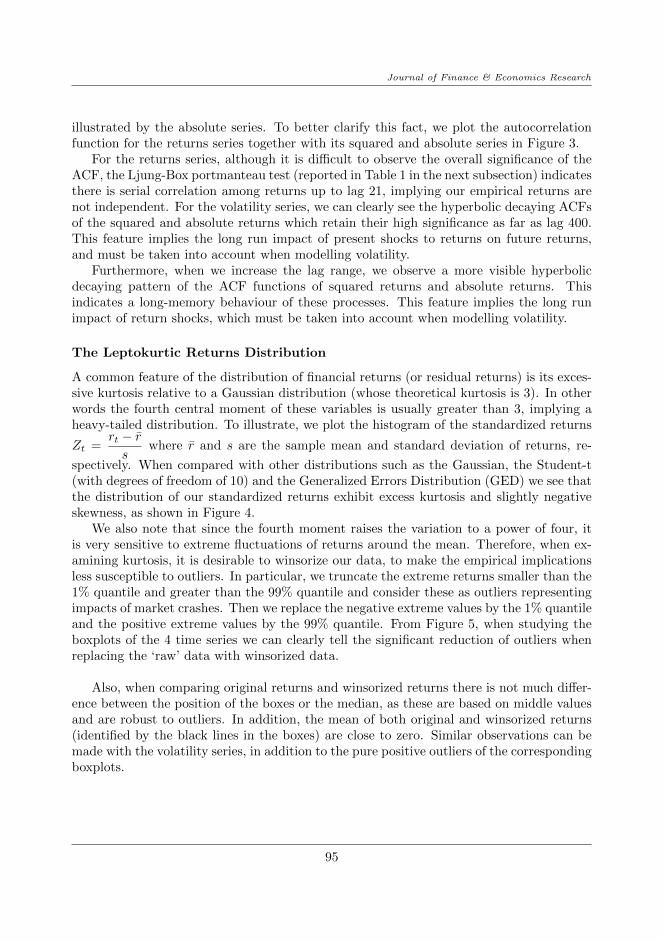
illustrated by the absolute series. To better clarify this fact, we plot the autocorrelationfunction for the returns series together with its squared and absolute series in Figure 3.
For the returns series, although it is difficult to observe the overall significance of theACF, the Ljung-Box portmanteau test (reported in Table 1 in the next subsection) indicatesthere is serial correlation among returns up to lag 21, implying our empirical returns arenot independent. For the volatility series, we can clearly see the hyperbolic decaying ACFsof the squared and absolute returns which retain their high significance as far as lag 400.This feature implies the long run impact of present shocks to returns on future returns,and must be taken into account when modelling volatility.
Furthermore, when we increase the lag range, we observe a more visible hyperbolicdecaying pattern of the ACF functions of squared returns and absolute returns. Thisindicates a long-memory behaviour of these processes. This feature implies the long runimpact of return shocks, which must be taken into account when modelling volatility.
The Leptokurtic Returns Distribution
A common feature of the distribution of financial returns (or residual returns) is its exces-sive kurtosis relative to a Gaussian distribution (whose theoretical kurtosis is 3). In otherwords the fourth central moment of these variables is usually greater than 3, implying aheavy-tailed distribution. To illustrate, we plot the histogram of the standardized returns
Zt =rt − rs
where r and s are the sample mean and standard deviation of returns, re-
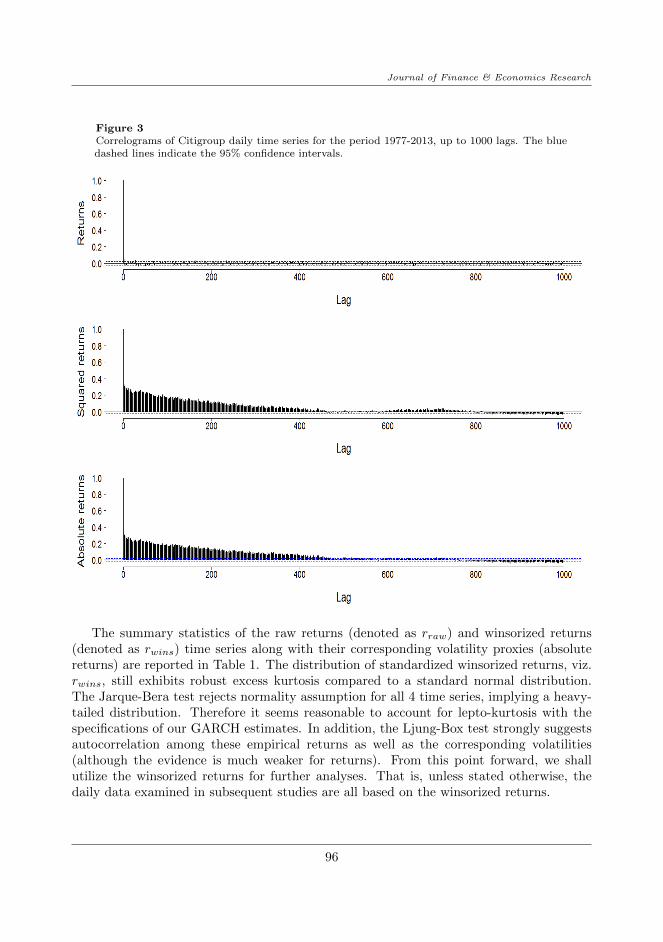
spectively. When compared with other distributions such as the Gaussian, the Student-t(with degrees of freedom of 10) and the Generalized Errors Distribution (GED) we see thatthe distribution of our standardized returns exhibit excess kurtosis and slightly negativeskewness, as shown in Figure 4.
We also note that since the fourth moment raises the variation to a power of four, itis very sensitive to extreme fluctuations of returns around the mean. Therefore, when ex-amining kurtosis, it is desirable to winsorize our data, to make the empirical implicationsless susceptible to outliers. In particular, we truncate the extreme returns smaller than the1% quantile and greater than the 99% quantile and consider these as outliers representingimpacts of market crashes. Then we replace the negative extreme values by the 1% quantileand the positive extreme values by the 99% quantile. From Figure 5, when studying theboxplots of the 4 time series we can clearly tell the significant reduction of outliers whenreplacing the ‘raw’ data with winsorized data.
Also, when comparing original returns and winsorized returns there is not much differ-ence between the position of the boxes or the median, as these are based on middle valuesand are robust to outliers. In addition, the mean of both original and winsorized returns(identified by the black lines in the boxes) are close to zero. Similar observations can bemade with the volatility series, in addition to the pure positive outliers of the correspondingboxplots.
95
Journal of Finance & Economics Research
Figure 3Correlograms of Citigroup daily time series for the period 1977-2013, up to 1000 lags. The bluedashed lines indicate the 95% confidence intervals.
The summary statistics of the raw returns (denoted as rraw) and winsorized returns(denoted as rwins) time series along with their corresponding volatility proxies (absolutereturns) are reported in Table 1. The distribution of standardized winsorized returns, viz.rwins, still exhibits robust excess kurtosis compared to a standard normal distribution.The Jarque-Bera test rejects normality assumption for all 4 time series, implying a heavy-tailed distribution. Therefore it seems reasonable to account for lepto-kurtosis with thespecifications of our GARCH estimates. In addition, the Ljung-Box test strongly suggestsautocorrelation among these empirical returns as well as the corresponding volatilities(although the evidence is much weaker for returns). From this point forward, we shallutilize the winsorized returns for further analyses. That is, unless stated otherwise, thedaily data examined in subsequent studies are all based on the winsorized returns.
96
Journal of Finance & Economics Research
Figure 4
Histogram of standardized daily Citigroup returns for period 1977-2013, with lines indicating
the fitted normal, student and GED density functions superimposed.
Test for Unit Root Non-Stationarity
It is observed that unit root non-stationary time series often exhibit slow decaying ACFssimilar to those of stationary long-memory processes. Therefore it might not be possible todistinguish the two type of processes relying only on the ACF (Brooks, 2002). To find outwhether our time series are non-stationary, we apply the Augmented Dickey-Fuller (ADF)test for unit root (see Dickey and Fuller (1979) and Hamilton (1994)).
Table 1Summary statistics for Citigroup daily data for the period 03 Jan 1977 to 31 Jul 2013
rraw |rraw | rwins |rwins | r2 wins
Mean 0.000189 0.0158056 0.0003052 0.014786 0.0004308
Median 0 0.0101181 0 0.010118 0.00010237Variance 0.000703 0.0004537 0.0004308 0.000212 6.92 × 10⁻⁷
Skewness -0.605176 6.576009 0.0246598 1.639483 3.174645Kurtosis 42.9454 84.3004 1.725833 2.58466 10.49374JB 710028.5 (0.0000) 2800229 (0.0000) 1147.528 (0.0000) 6706.388 (0.0000) 57869.75 (0.0000)LB (21) 144.31 (0.0000) 17018.05 (0.0000) 52.3834 (0.0000) 13161.6 (0.0000) 14189.44 (0.0000)p-values are reported in parentheses. JB, LB(21) indicate the Jargue-Bera and Ljung-Box statistics, respectively.
97

Journal of Finance & Economics Research
Figure 5Boxplots of daily time series of Citigroup for period 1977-2013. The black line indicates the median. Thenumber of outliers (or the length of the whiskers) is reduced significantly with the winsorized data. Herethe width of the boxes represents the Interquartile Range (IQR), or the difference between the upperquartile-UQ (or the 75% quantile) and lower quartile-LQ (or the 25% quantile). The lower and upper‘whiskers’ indicate the values equal LQ− 1.58× IQR and UQ+ 1.58× IQR, respectively. See e.g. McGill,Tukey, and Larsen (1978) and Chambers, Cleveland, Kleiner, and Tukey (1983). Any value falling outsideof the range implied by these whiskers is considered an outlier.
Specifically, we use the following model:
∆(Xt) = α+ βt+ γXt−1 +
p∑i=1
δi∆(Xt−i) + εt
Here α is a constant and β is the coefficient of the time trend. Including both coefficientsallow us to test for unit root with a drift and a deterministic time trend simultaneously.Unlike the original DF, the ADF adds the lagged differenced terms to account for upto order p serial correlation in the data generating process which could invalidate thestatistical inference of DF test. The ‘optimal’ number of augmenting lags (p) is determinedby minimizing the Akaike Information Criterion. ADF test statistic is the t-stat of the OLSestimate of γ. The null hypothesis of ADF test is γ = 0. Intuitively, when γ = 0 is notrejected, the time series is not stationary, and the lagged level (Xt−1) cannot be used topredict the lagged change (∆(Xt)).
As can be seen from Table 2 the ADF test rejects the null hypothesis at any level ofsignificance for all series. We can conclude that returns, squared returns and absolutereturns are stationary.
98

Journal of Finance & Economics Research
Table 2Augmented Dickey-Fuller test for stationarity indaily time series
Null hypothesis H0: γ = 0Test Eq. Series ADF stat Critical value*
Returns -67.142 1% -3.4593
Squared returns -45.963 5% -2.8738Absolute returns -46.95 10% -2.5732(*) The critical values are obtained from MacKinnon(1994)
In-sample Performance: Volatility Estimate with GARCHModels
We continue with analyses of GARCH frameworks covered in the previous sections, usingthe daily returns of Citigroup Inc. computed from the time series of closing prices, whichare adjusted for stock splits and dividends. We use 7341 observations from 01 Dec 1977 to31 Dec 2006 and refer to these as our in-sample data.
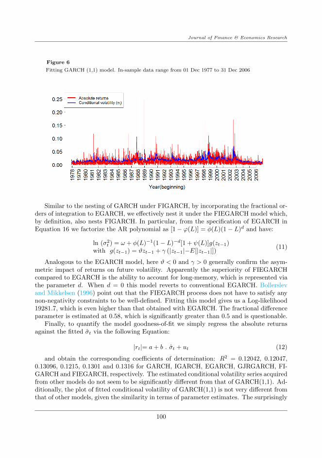
To illustrate the goodness-of-fit of GARCH(1,1), we first plot the fitted conditionalvolatility σt (formulated in previous sections) against in-sample absolute returns in Figure6. As can be seen, the overall shape of σ2
t tracks that of the actual data quite reasonably,save for the extreme values observed at several market crashes.
Comparing Models’ Performance
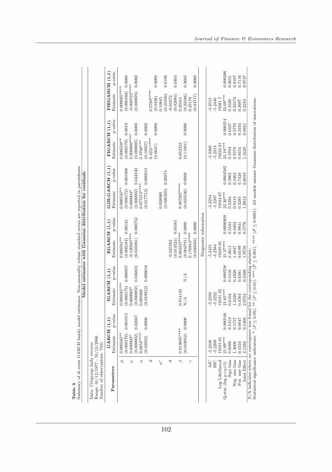
Model estimates and Diagnostic statistics are reported in Table 3 8. Most of the estimatedparameters are significant. The portmanteau Ljung-Box tests (up to lag 21) suggests noevidence of serial correlation among model residuals, indicating that these models seemto perform adequately. Interestingly, the EGARCH(1,1) yields the highest value of Log-likehood function compared to other GARCH models previously discussed, as well as thelowest value of Akaike Information Criterion (AIC) 9. Both of these indicators imply betterperformance of EGARCH. It should be noted that the FIGARCH(1,1) ranks second interms of performance and yield a estimated d = 0.4221 (corresponding to a Hurst indexof 0.9221) which is significant at the 1% level. Taken together, the improved performanceof EGARCH and FIGARCH imply that our volatility series does exhibit (i) a high degreeof long-memory and (ii) an asymmetric relationship with positive and negative returns.Inspired by these findings, we opt to specify yet another class of GARCH model designedto incorporate these two properties of financial volatility. The new model is called theFractionally Integrated Exponential ARCH (FIEGARCH), which was first proposed inNelson (1991) and then further examined by Bollerslev and Mikkelsen (1996).
8All estimates are obtained with the help of R package rugarch Ghalanos (2013), except for the resultsof FIGARCH and FIEGARCH (which are obtained using OXMetrics (Laurent & Peters, 2002).
9In its general form the AIC is defined as :AIC = 2k−2ln(L) where k is the number of model parametersand L is the maximized likelihood value of the estimated model (Akaike, 1974). For comparison, the modelwith the lowest AIC is chosen.
99
Journal of Finance & Economics Research
Figure 6
Fitting GARCH (1,1) model. In-sample data range from 01 Dec 1977 to 31 Dec 2006
Similar to the nesting of GARCH under FIGARCH, by incorporating the fractional or-ders of integration to EGARCH, we effectively nest it under the FIEGARCH model which,by definition, also nests FIGARCH. In particular, from the specification of EGARCH inEquation 16 we factorize the AR polynomial as [1− ϕ(L)] = φ(L)(1− L)d and have:
ln (σ2t ) = ω + φ(L)−1(1− L)−d[1 + ψ(L)]g(zt−1)
with g(zt−1) = ϑzt−1 + γ (|zt−1|−E[|zt−1|])(11)
Analogous to the EGARCH model, here ϑ < 0 and γ > 0 generally confirm the asym-metric impact of returns on future volatility. Apparently the superiority of FIEGARCHcompared to EGARCH is the ability to account for long-memory, which is represented viathe parameter d. When d = 0 this model reverts to conventional EGARCH. Bollerslevand Mikkelsen (1996) point out that the FIEGARCH process does not have to satisfy anynon-negativity constraints to be well-defined. Fitting this model gives us a Log-likelihood19281.7, which is even higher than that obtained with EGARCH. The fractional differenceparameter is estimated at 0.58, which is significantly greater than 0.5 and is questionable.
Finally, to quantify the model goodness-of-fit we simply regress the absolute returnsagainst the fitted σt via the following Equation:
|rt|= a+ b . σt + ut (12)
and obtain the corresponding coefficients of determination: R2 = 0.12042, 0.12047,0.13096, 0.1215, 0.1301 and 0.1316 for GARCH, IGARCH, EGARCH, GJRGARCH, FI-GARCH and FIEGARCH, respectively. The estimated conditional volatility series acquiredfrom other models do not seem to be significantly different from that of GARCH(1,1). Ad-ditionally, the plot of fitted conditional volatility of GARCH(1,1) is not very different fromthat of other models, given the similarity in terms of parameter estimates. The surprisingly
100
Journal of Finance & Economics Research
low in-sample R2 is a result of persistent underestimation of the fitted σ2t compared to daily
volatility proxied by absolute returns (see Figure 6). This, in turn, may be a result of thepresence of extreme volatility accompanying crises related to the 1980s housing bubble, the1987 market crash, the 2000s Internet bubble burst or the 2008 global financial distress,for which GARCH failed to provide good estimates.
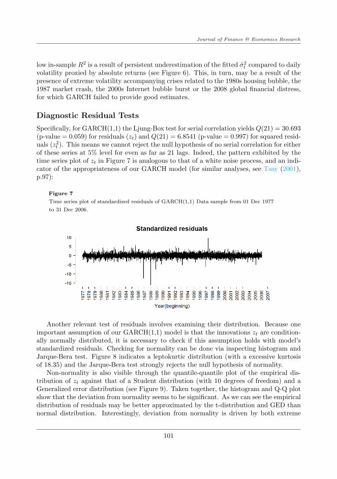
Diagnostic Residual Tests
Specifically, for GARCH(1,1) the Ljung-Box test for serial correlation yieldsQ(21) = 30.693(p-value = 0.059) for residuals (zt) and Q(21) = 6.8541 (p-value = 0.997) for squared resid-uals (z2
t ). This means we cannot reject the null hypothesis of no serial correlation for eitherof these series at 5% level for even as far as 21 lags. Indeed, the pattern exhibited by thetime series plot of zt in Figure 7 is analogous to that of a white noise process, and an indi-cator of the appropriateness of our GARCH model (for similar analyses, see Tsay (2001),p.97):
Figure 7
Time series plot of standardized residuals of GARCH(1,1) Data sample from 01 Dec 1977
to 31 Dec 2006.
Another relevant test of residuals involves examining their distribution. Because oneimportant assumption of our GARCH(1,1) model is that the innovations zt are condition-ally normally distributed, it is necessary to check if this assumption holds with model’sstandardized residuals. Checking for normality can be done via inspecting histogram andJarque-Bera test. Figure 8 indicates a leptokurtic distribution (with a excessive kurtosisof 18.35) and the Jarque-Bera test strongly rejects the null hypothesis of normality.
Non-normality is also visible through the quantile-quantile plot of the empirical dis-tribution of zt against that of a Student distribution (with 10 degrees of freedom) and aGeneralized error distribution (see Figure 9). Taken together, the histogram and Q-Q plotshow that the deviation from normality seems to be significant. As we can see the empiricaldistribution of residuals may be better approximated by the t-distribution and GED thannormal distribution. Interestingly, deviation from normality is driven by both extreme
101
Journal of Finance & Economics Research
Table
3S
um
mary
of
di
eren
tG
AR
CH
fam
ily
mod
eles
tim
ate
s.N
on
-norm
ali
tyro
bu
stst
an
dard
erro
rsare
rep
ort
edin
pare
nth
eses
Modelestim
ate
swith
Gaussian
distrib
ution
forresiduals
Data
:C
itig
rou
pd
ail
yre
turn
sR
an
ge:
01/12/1977
-31/12/2006
Nu
mb
erof
ob
serv
ati
on
s:7341
Param
ete
rs
GARCH
(1,1)
IGARCH
(1,1)
EGARCH
(1,1)
GJR-G
ARCH
(1,1)
FIG
ARCH
(1,1)
FIE
GARCH
(1,1)
Est
imate
p-v
alu
eE
stim
ate
p-v
alu
eE
stim
ate
p-v
alu
eE
stim
ate
p-v
alu
eE
stim
ate
p-v
alu
eE
stim
ate
p-v
alu
e
µ0.0
00585**
0.0
00585***
0.0
00591**
0.0
00535**
0.0
00559**
0.0
00685****
(0.0
00178)
0.0
01015
(0.0
00175)
0.0
00857
(0.0
00184)
0.0
0134
(0.0
00172)
0.0
01908
(0.0
00179)
0.0
019
(0.0
00166)
0.0
000
ω0.0
00003*
0.0
00003*
-0.1
20987***
0.0
00004*
0.0
00009****
-0.0
00723****
(0.0
00002)
0.0
2667
(0.0
00002)
0.0
36831
(0.0
35901)
0.0
00752
(0.0
00002)
0.0
44130
(0.0
00005)
0.0
000
(0.0
00076)
0.0
000
α0.0
853****
0.0
85866
0.0
77213****
0.3
768***
(0.0
2033)
0.0
000
(0.0
19912)
0.0
00016
(0.0
17713)
0.0
00013
(0.1
0057)
0.0
002
d0.4
221****
0.5
769****
(0.0
631)
0.0
000
(0.0
436)
0.0
000
α∗
0.0
28980
0.1
0845
(0.0
26205)
0.2
6874
(0.2
1856)
0.6
198
ϑ-0
.025562
-0.0
4273
(0.0
13324)
0.0
5561
(0.0
2084)
0.0
404
β0.9
13695****
0.9
14134
0.9
83537****
0.9
07297****
0.6
52333
0.2
0311
(0.0
19052)
0.0
000
N/A
N/A
(0.0
04791)
0.0
000
(0.0
23546)
0.0
000
(0.1
1091)
0.0
000
(0.2
2586)
0.3
685
γ0.1
76913****
0.2
5170
(0.0
30585)
0.0
000
(0.0
4717)
0.0
000
Dia
gn
ost
icin
form
ati
on
AIC
-5.2
246
-5.2
250
-5.2
431
-5.2
254
-5.2
360
-5.2
512
BIC
-5.2
209
-5.2
222
-5.2
384
-5.2
207
-5.2
313
-5.2
446
Log
Lik
elih
ood
19181.0
119181.3
519249.9
519184.8
719233.8
119281.7
Q-s
tat
(lag
p+
q+
5)
21.8
9***
0.0
00548
21.8
5***
0.0
00558
21.3
7***
0.0
006909
22.3
0***
0.0
004582
23.1
6***
0.0
00314
22.6
9***
0.0
00386
Sig
nb
ias
0.6
099
0.5
419
0.6
104
0.5
416
0.2
613
0.5
344
0.5
294
0.5
965
0.4
764
0.6
337
0.4
328
0.6
651
Neg
.si
zeb
ias
1.3
606
0.1
737
1.3
329
0.1
826
1.4
047
0.1
602
0.9
419
0.3
463
0.5
576
0.5
770
0.2
3172
0.8
167
Pos.
size
bia
s0.4
334
0.6
647
0.4
564
0.6
481
0.0
199
0.9
841
0.3
285
0.7
426
0.9
455
0.3
444
0.3
697
0.7
116
Join
tE
ffec
t2.1
293
0.5
460
2.0
754
0.5
569
1.9
750
0.5
776
1.0
012
0.8
010
1.3
420
0.6
921
0.2
233
0.9
737
N/A
ind
icate
sw
her
en
oco
nver
gen
cew
as
fou
nd
for
the
corr
esp
on
din
gst
ati
stic
.S
tati
stic
al
sign
ifica
nce
ind
icato
rs:
*(P≤
0.0
5),
**
(P≤
0.0
1),
***
(P≤
0.0
01),
****
(P≤
0.0
001).
All
mod
els
ass
um
eG
au
ssia
nd
istr
ibu
tion
of
inn
ovati
on
s.
102

Journal of Finance & Economics Research
negative and positive returns shocks, which is consistent with the fact that GARCH (1,1)is unable to discriminate between the signs of shocks. Deviation from t-distribution andGED, on the other hand, seems to be mostly driven by large positive shocks.
Figure 8
Histogram and descriptive statistics of standardized residuals for GARCH(1,1).
Density curves from 3 distributions: normal, Student and GED with comparable mean and variance
are superimposed.
Given these insights, we proceed to adjust our original assumption of normality andre-estimate the GARCH models with Maximum likelihood functions corresponding to theStudent t-distribution and Generalized errors distribution (note that our original estimatesare robust to non-normality thanks to robust standard deviation proposed by Bollerslevand Wooldridge (1992). Other conditions are preserved for re-estimation. Results are re-ported in Tables 4 and Table 5 for t-distribution and GED, respectively. Overall we observeimprovement in terms of higher Log-likelihood values: for example, for GARCH(1,1) themaximum Log-likelihood increases from 19181.01 with Normal distribution to 19642.62 fort-distribution and 19587.99 for GED. Likewise the AIC decreases from −5.22 to −5.35 and−5.33. Estimated values of main parameters and corresponding significance do not changedramatically. However, this seemingly improved goodness-of-fit (with respect to empiri-cal returns data) is not manifest in increased R-squared from regressing absolute returnsagainst σ2
t . In particular, with GARCH(1,1) we obtain R2 = 0.1202 for t-distribution andR2 = 0.1200 for GED (compared to R2 = 0.12042 for normal distribution). However,all of the statistics associated with estimates for FIGARCH(1,1) model do not convergewhen the GED is adopted. The same observation is made with FIEGARCH(1,1) for bothStudent and GED distribution specifications, which is why we do not report the estimates
103

Journal of Finance & Economics Research
of this model in these two cases. Nevertheless, throughout the various specifications ofresiduals’ distribution, FIGARCH(1,1) exhibits a very high degree of fractional differenceparameter (around 0.42).
Figure 9Q-Q plots of residuals’ distribution against normal distribution (top), t-distribution (middle)and GED (bottom). Red line indicates identity line.
Out-of-sample Performance: Daily Volatility vs. Real-ized Volatility
The primary value of a time series model lies in its ability to provide reliable approxi-mations of the modelled variable, both in-sample (where data are used to estimate modelparameters) and out-of-sample (where the model is updated with new data and producesforecasts). Here we illustrate how high-frequency data is used to construct a ‘realized’volatility measure which may provide a better approximation to the latent volatility vari-able. For comparative purposes, in the first part of the subsequent analysis we adopt the
104

Journal of Finance & Economics Research
approach of Andersen and Bollerslev (1998) and Hansen and Lunde (2005). In line withthese authors, we find some evidence for the credibility of GARCH (1,1) model.
It should be noted that, throughout the section, we focus on ‘ex-post’ one-period-aheadforecasts when evaluating model performance out-of-sample, meaning we use known returnsdata to update our estimated GARCH model and get the forecasts of volatility (a techniqueknown as ‘rolling forecast’). Although these forecasts have less practical value than the‘ex-ante’ forecasts (e.g. rather than using known returns to get volatility forecasts, we mayfirst forecast returns themselves), this is a standard approach which provides an objectiveand direct assessment of model performance.
Study Design
To begin, we use a more general notation of returns proposed by Andersen and Bollerslev(1998), which incorporates the sampling frequency m:
r(m),t = pt − pt−1/m where t = 0, 1/m, 2/m, . . .
in which pt denotes the logarithmic price. Given the sampling rate m, we define {r(m),t} asthe discretely observed time series of continuously compounded returns withm observationsper day. The instantaneous returns process is then defined as rt ≡ r(∞),t ≡ dpt. Whenm = 1 we have the daily returns, which represents the standard frequency in many studies.
Following Andersen and Bollerslev (1998) we model the (1-period) daily volatility usingthe generalized GARCH (1,1) specification:
σ2(m),t = ω(m) + α(m).r
2(m),t−1/m + β(m).σ
2(m),t−1/m
r(m),t = σ(m),t.z(m),t
where ω(m) > 0, α(m) ≥ 0, β(m) ≥ 0z(m),t ∼ i.i.d N(0,1)where m = 1
(13)
Theoretically, if we have a correctly specified model, our forecast must equal the truereturn variance, i.e.:
E(r2t+1) = E(|rt+1|2) = E(u2
t+1) ≡ σ2t+1
This motivates a direct way to evaluate GARCH forecast performance, that is, to usesome type of MSE (mean squared errors)-based metrics to test for the null hypothesis:E(σ2
t+1−Var[rt+1]) = 0. To do this the most popular approach is analogous to Mincer andZarnowitz (1969)’s method of evaluating conditional mean forecasts (but in this contextwe need to evaluate conditional variance forecasts instead). In particular, we simply needto regress some ex-post realized volatility measurement on the estimated values obtainedfrom GARCH (1,1) as follows:
r2(m),t+1/m = a(m) + b(m) . σ
2(m),t+1/m + u(m),t+1/m (14)
With the method outlined, the next step is to choose an appropriate ex-post volatilityproxy. Andersen and Bollerslev (1998) criticized the use of squared returns as a volatil-ity proxy. They show that using this quantity results in a ‘systematically’ poor forecast
105

Journal of Finance & Economics Research
performance, because daily squared return is an unbiased, but very noisy estimator of thetrue latent volatility. This is evident in a ‘disappointingly’ low R-squared obtained whenregressing this proxy on the forecasts, as commonly observed in numerous contemporarypapers. In hope of reducing the degree of misspecification associated with using squaredreturns by a power of 2, we opt for using absolute returns. This is also consistent with theview of volatility as standard deviation rather than variance. In addition, Taylor (1986)’sfindings suggest that better forecasts of volatility were provided by models using absolutereturns compared to squared returns. This might be a result of absolute returns displayinghigher degree of long-memory than squared returns, which motivates direct modelling ofvolatility from absolute returns (See e.g. Ding and Granger (1996) and Vuorenmaa (2005)).Furthermore, as pointed out by Vuorenmaa (2005), since the logarithmic squared value ofa close-to-zero return would be negative, it is less favourable to be used as volatility proxycompared to an absolute return, which is more robust to this kind of ‘inlier’ problem. Theabove arguments have been largely verified with stock data, at the very least.
Application
We start with estimating the GARCH (1,1) model (specified in Equation 13), using in-sample data based on daily returns of Citigroup, Inc. from 01 Dec 1977 to 31 Dec 2006.Next, we update the estimated model with out-of-sample daily returns from 03 Jan 2007 to31 Dec 2007 and get the rolling forecast of volatility (denoted as σ(m),t+1/m). Consequently,our one-step ahead GARCH(1,1) volatility forecasts are computed for the period of 250working days of the year 2007 (excluding weekends and holidays for their insignificanttrading activities). We then proceed to replace the fitted/forecast variance in equation 14with these values. In other words we modify Andersen and Bollerslev (1998)’s approachby regressing absolute returns on forecast standard deviation instead of regressing squaredreturns on forecast variances 10:
|r(m),t+1/m|= a(m) + b(m) . σ(m),t+1/m + ε(m),t+1/m (15)
Substituting absolute daily returns (m = 1) into this generalization we have:
|r(1),t+1|= a(1) + b(1) . σ(1),t+1 + ε(1),t+1 (16)
The R-squared value of Equation (16) (R2(1)) can be viewed as a simple indicator of how
well our estimates of volatility can explain the variability in the ex-post returns which, intheory, can not be observed. The problem remains, as discussed earlier, that traditionaldaily proxies of volatility (e.g. squared residual returns, squared returns, absolute returns)may not be adequate. In particular, as can be seen in Table 4, using daily absolutereturns as volatility proxy (or the dependent variable in Equation 16) suggests that ourGARCH(1,1) model only explains 13.9% of the daily variability of returns. When using
10The former specification is also adopted by (Jorion, 1995). A viable alternative would be to comparevolatility forecasts with ex-post returns shocks (or residual returns) out-of-sample. But as Tsay (2001)argued, using returns shocks as a measure of realized volatility may not be a good idea. A single realizationof the random variable u2t+1 is not adequate to provide an accurate estimate of the movement of day-by-dayvolatility (or Vart+1(ut)).
106

Journal of Finance & Economics Research
squared returns we obtain a decreased value: R2(1) = 0.0997, but this is still higher than the
corresponding R2 values reported in Andersen and Bollerslev (1998)’s exchange rate study,i.e. 0.047for the Deutsche Mark/U.S. Dollar (DM-$) and 0.026 for Japanese Yen/U.S.Dollar (U-$) rates.
All things considered, these results suggest that absolute returns may provide a moreappropriate volatility proxy than squared returns. However, regardless of the proxies used,the low R2
(1) and a poor out-of-sample fit are to be expected, as both proxies are noisyestimators of true volatility process. In defence of the GARCH model, Andersen andBollerslev (1998) assert that the use of these noisy proxies distort our perception of GARCHforecasts performance, because “[...] Rational financial decision making hinges on theanticipated future volatility and not the subsequent realized squared returns. Under the nullhypothesis that the estimated GARCH(1,1) model constitutes the correct specification, thetrue return variance is, by definition, identical to the GARCH volatility forecast.” (p.890).
Realized Volatility Proxy Constructed from Intraday Returns
The above arguments imply that to obtain meaningful forecast evaluation we first need toacquire a better volatility estimate. According to the theory of quadratic variation (SeeKaratzas and Shreve (1991)), in principle, the cumulative squared intraday returns providebetter approximation to ex-post volatility at higher sampling rate:
limm→∞(
∫ 1
0
σ2t+τdτ −
m∑j=1
r2(m),t+j/m) = 0 (17)
in which
∫ 1
0
σ2t+τdτ denotes the continuous time volatility measure and r2
(m),t+j/m is
the length j/m period squared return. Motivated by this proposition, Hansen and Lunde(2005) show that when intraday returns are uncorrelated we have an unbiased estimatorof σ2
t simply by summing intraday squared returns:
σ2(m),t ≡
m∑j=1
r2(m),t+j/m
E[σ2
(m),t
]= E(r2
t ) = E[σ2
(1),t
] (18)
Ideally we would choose m close to infinity. In practice, irregularly spaced price re-alizations would render computing ‘continuous’ measurement at an infinite sampling rateinfeasible. Furthermore, various microstructure effects may result in negative serial corre-lation among returns (Dacorogna et al., 2001). Many researchers suggest 5 minutes as theoptimal sampling interval. Therefore we opt for using a realized volatility measures com-puted from intraday returns recorded every 5 minutes for the year 2007. These returns arecalculated from a value weighted average of tick-by-tick prices provided by the AustralianSecurities Industry Research Centre of Asia-Pacific (SIRCA).
107
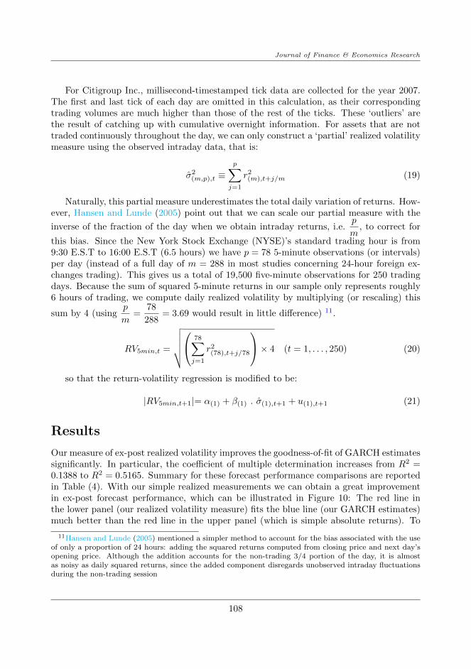
Journal of Finance & Economics Research
For Citigroup Inc., millisecond-timestamped tick data are collected for the year 2007.The first and last tick of each day are omitted in this calculation, as their correspondingtrading volumes are much higher than those of the rest of the ticks. These ‘outliers’ arethe result of catching up with cumulative overnight information. For assets that are nottraded continuously throughout the day, we can only construct a ‘partial’ realized volatilitymeasure using the observed intraday data, that is:
σ2(m,p),t ≡
p∑j=1
r2(m),t+j/m (19)
Naturally, this partial measure underestimates the total daily variation of returns. How-ever, Hansen and Lunde (2005) point out that we can scale our partial measure with the
inverse of the fraction of the day when we obtain intraday returns, i.e.p
m, to correct for
this bias. Since the New York Stock Exchange (NYSE)’s standard trading hour is from9:30 E.S.T to 16:00 E.S.T (6.5 hours) we have p = 78 5-minute observations (or intervals)per day (instead of a full day of m = 288 in most studies concerning 24-hour foreign ex-changes trading). This gives us a total of 19,500 five-minute observations for 250 tradingdays. Because the sum of squared 5-minute returns in our sample only represents roughly6 hours of trading, we compute daily realized volatility by multiplying (or rescaling) this
sum by 4 (usingp
m=
78
288= 3.69 would result in little difference) 11.
RV5min,t =
√√√√√ 78∑j=1
r2(78),t+j/78
× 4 (t = 1, . . . , 250) (20)
so that the return-volatility regression is modified to be:
|RV5min,t+1|= α(1) + β(1) . σ(1),t+1 + u(1),t+1 (21)
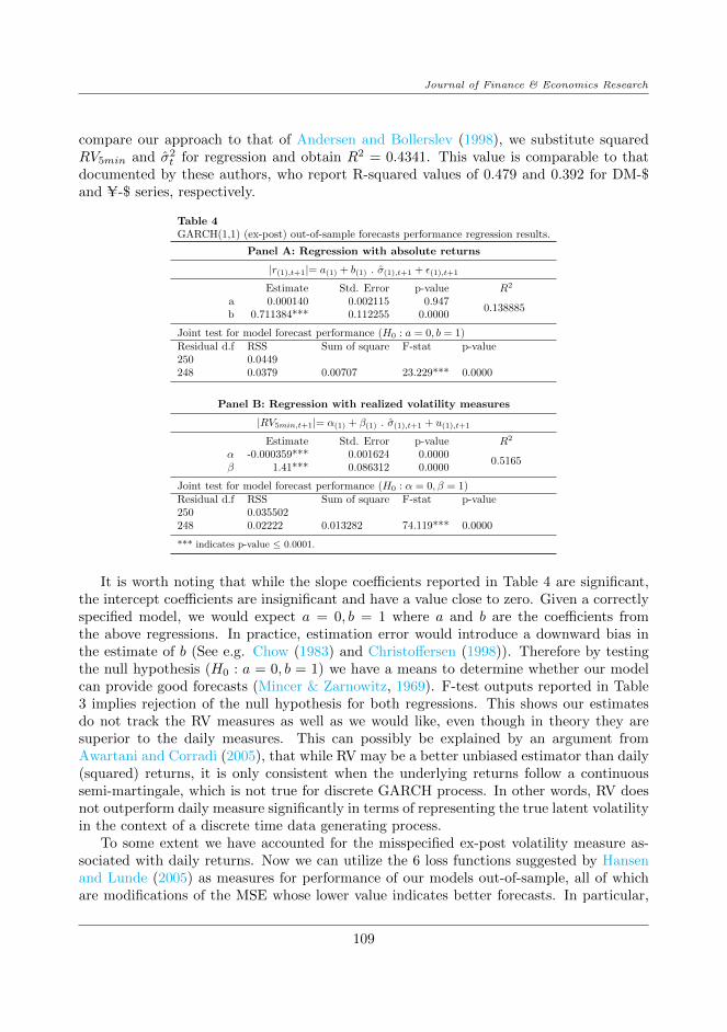
Results
Our measure of ex-post realized volatility improves the goodness-of-fit of GARCH estimatessignificantly. In particular, the coefficient of multiple determination increases from R2 =0.1388 to R2 = 0.5165. Summary for these forecast performance comparisons are reportedin Table (4). With our simple realized measurements we can obtain a great improvementin ex-post forecast performance, which can be illustrated in Figure 10: The red line inthe lower panel (our realized volatility measure) fits the blue line (our GARCH estimates)much better than the red line in the upper panel (which is simple absolute returns). To
11Hansen and Lunde (2005) mentioned a simpler method to account for the bias associated with the useof only a proportion of 24 hours: adding the squared returns computed from closing price and next day’sopening price. Although the addition accounts for the non-trading 3/4 portion of the day, it is almostas noisy as daily squared returns, since the added component disregards unobserved intraday fluctuationsduring the non-trading session
108
Journal of Finance & Economics Research
compare our approach to that of Andersen and Bollerslev (1998), we substitute squaredRV5min and σ2
t for regression and obtain R2 = 0.4341. This value is comparable to thatdocumented by these authors, who report R-squared values of 0.479 and 0.392 for DM-$and U-$ series, respectively.
Table 4GARCH(1,1) (ex-post) out-of-sample forecasts performance regression results.
Panel A: Regression with absolute returns
|r(1),t+1|= a(1) + b(1) . σ(1),t+1 + ε(1),t+1
Estimate Std. Error p-value R2
a 0.000140 0.002115 0.9470.138885
b 0.711384*** 0.112255 0.0000
Joint test for model forecast performance (H0 : a = 0, b = 1)Residual d.f RSS Sum of square F-stat p-value250 0.0449248 0.0379 0.00707 23.229*** 0.0000
Panel B: Regression with realized volatility measures
|RV5min,t+1|= α(1) + β(1) . σ(1),t+1 + u(1),t+1
Estimate Std. Error p-value R2
α -0.000359*** 0.001624 0.00000.5165
β 1.41*** 0.086312 0.0000
Joint test for model forecast performance (H0 : α = 0, β = 1)Residual d.f RSS Sum of square F-stat p-value250 0.035502248 0.02222 0.013282 74.119*** 0.0000
*** indicates p-value ≤ 0.0001.
It is worth noting that while the slope coefficients reported in Table 4 are significant,the intercept coefficients are insignificant and have a value close to zero. Given a correctlyspecified model, we would expect a = 0, b = 1 where a and b are the coefficients fromthe above regressions. In practice, estimation error would introduce a downward bias inthe estimate of b (See e.g. Chow (1983) and Christoffersen (1998)). Therefore by testingthe null hypothesis (H0 : a = 0, b = 1) we have a means to determine whether our modelcan provide good forecasts (Mincer & Zarnowitz, 1969). F-test outputs reported in Table3 implies rejection of the null hypothesis for both regressions. This shows our estimatesdo not track the RV measures as well as we would like, even though in theory they aresuperior to the daily measures. This can possibly be explained by an argument fromAwartani and Corradi (2005), that while RV may be a better unbiased estimator than daily(squared) returns, it is only consistent when the underlying returns follow a continuoussemi-martingale, which is not true for discrete GARCH process. In other words, RV doesnot outperform daily measure significantly in terms of representing the true latent volatilityin the context of a discrete time data generating process.
To some extent we have accounted for the misspecified ex-post volatility measure as-sociated with daily returns. Now we can utilize the 6 loss functions suggested by Hansenand Lunde (2005) as measures for performance of our models out-of-sample, all of whichare modifications of the MSE whose lower value indicates better forecasts. In particular,
109

Journal of Finance & Economics Research
given n = 250 we would have:
MSE1 = n−1
n∑t=1
(σt − ht)2 ; MSE2 = n−1n∑t=1
(σ2t − h2
t )2
PSE = n−1
n∑t=1
(σ2t − h2
t )2h−4t ; R2LOG = n−1
n∑t=1
[ log(σ2t h−2t )]
2
MAD1 = n−1
n∑t=1
|σt − ht| ; MAD2 = n−1n∑t=1
|σ2t − h2
t |
(22)
where σt is the estimated volatility and ht indicates our ex-post measures (RV5min).Results are reported in Table 4, which shows little difference between the models, althoughthere is slightly better performance of GJR-GARCH (1,1). Overall, all 4 models examinedprovide relatively good out-of-sample forecasts. It seems that models accounting for asym-metry do have slightly better performance, both in and out-of-sample. Again the resultsneed cautious consideration regarding the limit of data range.
Table 5Comparing out-of-sample forecasts performance for different GARCH models, using6 metrics suggested by Hansen and Lunde (2005).
Forecast performance metricsModel MSE1 MSE2 PSE R2LOG MAD1 MAD2
GARCH(1,1) 0.00014200 8.20×10⁻⁷ 0.259646 0.720293 0.007773 0.000454IGARCH(1,1) 0.00014139 8.17×10⁻⁷ 0.260498 0.719489 0.00776 0.000453EGARCH(1,1) 0.00013793 8.07×10⁻⁷ 0.255495 0.690906 0.00769 0.000450GJR-GARCH(1,1) 0.00013171 7.74×10⁻⁷ 0.250268 0.668722 0.00750 0.000439
Figure 10
Comparing one-step ahead daily forecasts from GARCH(1,1) model (σ(1),t+1) with corresponding
absolute returns (top) and realized volatility measure computed from 5-minute returns (bottom).
Data sample ranges from 01 Jan 2007 to 31 Dec 2007.
110

Journal of Finance & Economics Research
Concluding Remarks
In the most recent decades, the availability of financial data has played an increasingly in-dispensable role in facilitating the development of quantitative models aiming to constructvolatility theories. This point of view can be underscored by simply considering the parallelevolution of data frequencies and the corresponding diversity of such models. Linear modelfamilies such as the Autoregressive Integrated Moving Average (ARIMA) had been usedto model monthly or yearly data from the 1970s. When daily and weekly data becameavailable in the 1980s, discoveries of varying conditional variance of returns called for thenon-linear branch of ARCH models. Recently, even the conventional GARCH did little interms of explaining the new range of properties extracted from the high-frequency data.
Living up to their celebrated reputation, the various GARCH models examined in thisstudy do provide decent in-sample volatility estimates, as evidenced by the strong perfor-mance of the model residuals in diagnostic tests. Overall, the empirical evidence presentedin this paper indicates that to some extent, the volatility process is predictable and/or canbe effectively modelled by GARCH models. In addition, this simple example illustrates theimportant role of intraday data in constructing improved ex-post volatility measurements.The results, although being more or less consistent with previous studies, remain some-what inconclusive, considering the (discrete) out-of-sample data range is relatively smallcompared to the large in-sample data range. This observation calls for further investigationusing longer time frame of high-frequency data.
Given the advantage of our approach, it is worthwhile to acknowledge its shortcomings.Our study, for all intents and purposes, aims to explore the volatility structure of only onecompany, Citigroup Inc., which, despite having a heavily traded stock reflecting importantmarket fluctuations, may possess unique capital structure properties that affect our findingsand make them biased. In addition, for many reasons the firm was highly impacted by theGFC, more than any other financial service company. This means our results may havelimited general validity. On the other hand, the fact remains that it is the special position ofCitigroup in the global finance system that provides us with a worthy candidate to studythe inter-relationship between returns and volatility. Preferably, to extend our paper’simplications to a wider group, in the future, we could conduct event studies to focus onspecific periods that can be related to the company’s financial structure, or we could studya group of companies that share Citigroup’s intrinsic characteristics. Alternatively, wecould organize similar investigations on various indexes, from both developed and emergingmarkets, to draw more general conclusions.
111
Journal of Finance & Economics Research
References
Akaike, H. (1974). A new look at the statistical model identification. IEEE Transactionson Automatic Control , 19 (6), 716-723.
Andersen, T. G., & Bollerslev, T. (1997). Heterogeneous information arrivals and returnvolatility dynamics: Uncovering the long run in high frequency returns. Journal ofFinance, 52 (3), 975-1005.
Andersen, T. G., & Bollerslev, T. (1998). Answering the skeptics: Yes, standard volatilitymodels do provide accurate forecasts. International Economic Review , 39 (4), 885-905.
Andersen, T. G., Bollerslev, T., & Cai, J. (2000). Intraday and interday volatility in theJapanese stock market. Journal of International Financial Markets, Institutions andMoney , 10 (2), 107-130.
Andersen, T. G., Bollerslev, T., Diebold, F. X., & Labys, P. (1999). (Understanding, Op-timizing, Using and Forecasting) Realized Volatility and Correlation (Working PaperSeries No. 99-061). New York University, Leonard N. Stern School of Business. Re-trieved from http://ideas.repec.org/p/fth/nystfi/99-061.html
Awartani, B. M. A., & Corradi, V. (2005). Predicting the volatility of the S&P500stock index via GARCH models: the role of asymmetries. International Journal ofForecasting , 21 (1), 167-183.
Barndorff-Nielsen, O. E., & Shephard, N. (2002). Econometric analysis of realized volatilityand its use in estimating stochastic volatility models. Journal of the Royal StatisticalSociety. Series B (Statistical Methodology), 64 (2), 253-280.
Bollerslev, T. (1986). Generalized Autoregressive Conditional Heteroskedasticity. Journalof Econometrics, 31 , 307-327.
Bollerslev, T., & Mikkelsen, H. O. (1996). Modeling and pricing long memory in stockmarket volatility. Journal of Econometrics, 73 (1), 151-184.
Bollerslev, T., & Wooldridge, J. M. (1992). Quasi-maximum likelihood estimation andinference in dynamic models with time-varying covariances. Econometric Reviews,11 (2), 143–172.
Boubaker, H., & Raza, S. A. (2017, may). A wavelet analysis of mean and volatilityspillovers between oil and BRICS stock markets. Energy Economics, 64 , 105–117.Retrieved from https://doi.org/10.1016%2Fj.eneco.2017.01.026 doi: 10.1016/j.eneco.2017.01.026
Brooks, C. (2002). Introductory Econometrics for Finance. Cambridge, U.K: CambridgeUniversity Press.
Campbell, J. Y., Lo, A. W., & MacKinlay, A. C. (1997). The econometrics of financialmarkets. Princeton, N.J: Princeton University Press.
Chambers, J., Cleveland, W., Kleiner, B., & Tukey, P. (1983). Graphical methods for dataanalysis. Boston, MA: Duxury: Wadsworth International Group.
Chen, Z. (2014, oct). Index future trading, spot volatility and market efficiency. Journal ofManagement Sciences, 1 (2), 73–112. Retrieved from https://doi.org/10.20547%
2Fjms.2014.1401201 doi: 10.20547/jms.2014.1401201
112

Journal of Finance & Economics Research
Cheng, P., Roberts, L., & Wu, E. (2013). A wavelet analysis of returns on heavily tradedstocks during times of stress [Working paper]. (School of Economics and Finance,Victoria University of Wellington: Wellington, New Zealand.)
Chow, G. C. (1983). Econometrics. McGraw-Hill.Christensen, B. J., & Nielsen, M. (2007). The effect of long memory in volatility on stock
market fluctuations. The Review of Economics and Statistics, 89 (4), 684-700.Christoffersen, P. F. (1998). Evaluating interval forecasts. International Economic Review ,
39 (4), 841-862.Dacorogna, M. M., Gencay, R., Muller, U., Olsen, R. B., & Pictet, O. V. (2001). An
Introduction to High Frequency Finance. San Diego: Academic Press.Dickey, D. A., & Fuller, W. A. (1979). Distributions of the estimators for autoregressive
time series with a unit root. Journal of the American Statistical Association, 74 (366),427-431.
Diebold, F. X. (1988). Empirical Modeling of Exchange Rate Dynamics. New York:Springer-Verlag.
Ding, Z., & Granger, C. W. J. (1996). Modeling volatility persistence of speculativereturns: A new approach. Journal of Econometrics, 73 (1), 185-215.
Drost, F. C., & Nijman, T. E. (1993). Temporal aggregation of GARCH processes. Econo-metrica, 61 (4), 909-27.
Engle, R. F. (1982). Autoregressive Conditional Heteroscedasticity with estimates of thevariance of United Kingdom inflation. Econometrica, 50 (4), 987-1007.
Engle, R. F. (2001). GARCH 101: The use of ARCH/GARCH models in applied econo-metrics. The Journal of Economic Perspectives, 15 (4), 157-168.
Engle, R. F., & Patton, A. (2001). What good is a volatility model? Quantitative Finance,1 (2), 237-245.
Fama, E. F. (1965). The Behavior of stock market prices. The Journal of Business, 38 (1),34-105.
Fleming, J., & Kirby, C. (2011). Long memory in volatility and trading volume. Journalof Banking and Finance, 35 (7), 1714-1726.
Ghalanos, A. (2013). rugarch: Univariate GARCH models [Computer software manual].Retrieved from http://CRAN.R-project.org/package=rugarch (R package version1.2.2)
Glosten, L. R., Jagannathan, R., & Runkle, D. E. (1993). On the relation between theexpected value and the volatility of the nominal excess return on stocks. Journal ofFinance, 48 (5), 1779-1801.
Granger, C. W. J., Spear, S., & Ding, Z. (2000). Stylized facts on the temporal anddistributional properties of absolute returns: An update. Statistics and Finance: AnInterface, 97-120.
Hamilton, J. D. (1994). Time Series Analysis. Princeton, N.J: Princeton University Press.Hansen, P. R., & Lunde, A. (2005). A forecast comparison of volatility models: does
anything beat a GARCH (1,1)? Journal of Applied Econometrics, 20 (7), 873-889.Hull, J. (2006). Options, Futures, and Other Derivatives. Upper Saddle River, N.J: Pearson
Education.
113
Journal of Finance & Economics Research
Hull, J., & White, A. (1996). Hull-White on Derivatives: a Compilation of Articles.London: Risk Publications.
Jensen, M. J., & Whitcher, B. (2000). Time-varying long-memory in volatility: Detectionand estimation with wavelets [Working paper]. Retrieved from http://citeseerx
.ist.psu.edu/viewdoc/summary?doi=10.1.1.40.4242
Jorion, P. (1995). Predicting volatility in the foreign exchange market. Journal of Finance,50 (2), 507-528.
Karatzas, I., & Shreve, S. E. (1991). Brownian Motion and Stochastic Calculus. New York:Springer-Verlag.
Laurent, S., & Peters, J.-P. (2002). G@RCH 2.2: An Ox package for estimating andforecasting various ARCH models. Journal of Economic Surveys(16), 447-485.
Lo, A. W. (1991). Long-term memory in stock market prices. Econometrica, 59 (5),1279-1313.
Mandelbrot, B. (1963). The variation of certain speculative prices. The Journal of Busi-ness, 36 (4), 394-419.
Martens, M. (2001). Forecasting daily exchange rate volatility using intraday returns.Journal of International Money and Finance, 20 (1), 1-23.
McGill, R., Tukey, J. W., & Larsen, W. A. (1978). Variations of box plots. The AmericanStatistician, 32 (1), 12–16.
Melino, A. (1991). Estimation of continuous-time models in finance [Working paper].(Department of Economics and Institute for Policy Analysis, University of Toronto.)
Merton, R. (1980). On estimating the expected return on the market: An exploratoryinvestigation. Journal of Financial Economics, 8 (4), 323-361.
Mincer, J. A., & Zarnowitz, V. (1969). The Evaluation of Economic Forecasts. NationalBureau of Economic Research, Inc.
Muller, U. A., Dacorogna, M. M., Dave, R. D., Pictet, O. V., Olsen, R. B., & Ward, J. R.(1995). Fractals and intrinsic time: a challenge to econometricians. In Discussionpaper presented at the 1993 International Conference of the Applied EconometricsAssociation. Retrieved from http://ideas.repec.org/p/wop/olaswp/ 009.html
Nelson, D. B. (1991). Conditional heteroskedasticity in asset returns: A new approach.Econometrica, 59 (2), 347-70.
Nelson, D. B. (1992). Filtering and forecasting with misspecified ARCH models . Journalof Econometrics, 52 (1), 61-90.
Poon, S.-H., & Granger, C. W. (2003). Forecasting volatility in financial markets: Areview. Journal of Economic Literature, 41 (2), 478-539.
Securities Industry Research Centre of Asia-Pacific. (Ongoing). Thomson Reuters TickHistory. Retrieved from https://www.sirca.org.au/ ([Accessed in March 2013.])
Taylor, S. (1986). Modelling Financial Time Series. New York: John Wiley & Sons.Taylor, S. (2005). Asset Price Dynamics, Volatility, and Prediction. Princeton, N.J.:
Princeton University Press.Tsay, R. S. (2001). Analysis of Financial Time Series. New York: John Wiley & Sons.Vuorenmaa, T. A. (2005). A wavelet analysis of scaling laws and long-memory in stock
market volatility (Research Discussion Papers No. 27/2005). Bank of Finland. Re-trieved from http://ideas.repec.org/p/hhs/bofrdp/2005 027.html
114