Embed Size (px)
Citation preview
Chapter 8
1
Chapter 8
Mrs. Daniel‐ AP Statistics
Section 8.1
Confidence Intervals: The Basics
Section 8.1Confidence Intervals: The Basics
After this section, you should be able to…
INTERPRET a confidence level
INTERPRET a confidence interval in context
DESCRIBE how a confidence interval gives a range of plausible values for the parameter
DESCRIBE the inference conditions necessary to construct confidence intervals
EXPLAIN practical issues that can affect the interpretation of a confidence interval
Confidence Intervals
In this chapter, we’ll learn one method of statistical inference –confidence intervals – so we may
• Estimate the value of a parameter from a sample statistic
• Calculate probabilities that would describe what would happen if we used the inference method many times.
In Chapter 7 we assumed we knew the population parameter; however, in many real life situations, it is impossible to know the population parameter. Can we really weigh all the uncooked burgers in the US? Can we really measure the weights of all US citizens?
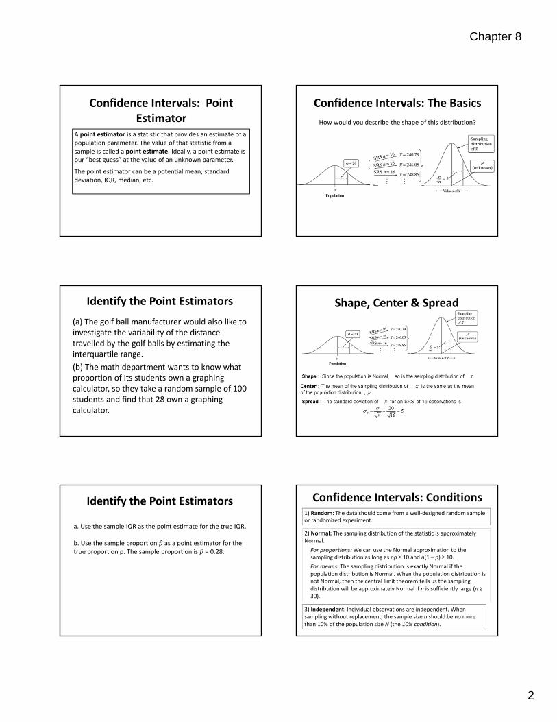
The Idea of a Confidence Interval
For example: Based on our SRS we find the mean height of 16 year girls to be 65.28 inches. Is the value of the population mean µ exactly 65.28 inches? Probably not.
However, since the sample mean is 65.28, we could guess that µ is “somewhere” around 65.28. How close to 240.79 is µ likely to be?
Confidence Intervals: The Basics
Chapter 8
2
Confidence Intervals: Point Estimator
A point estimator is a statistic that provides an estimate of a population parameter. The value of that statistic from a sample is called a point estimate. Ideally, a point estimate is our “best guess” at the value of an unknown parameter.
The point estimator can be a potential mean, standard deviation, IQR, median, etc.
Identify the Point Estimators
(a) The golf ball manufacturer would also like to investigate the variability of the distance travelled by the golf balls by estimating the interquartile range.
(b) The math department wants to know what proportion of its students own a graphing calculator, so they take a random sample of 100 students and find that 28 own a graphing calculator.
Identify the Point Estimators
a. Use the sample IQR as the point estimate for the true IQR.
b. Use the sample proportion as a point estimator for the true proportion p. The sample proportion is = 0.28.
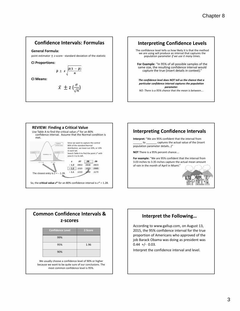
Confidence Intervals: The Basics
How would you describe the shape of this distribution?
Shape, Center & Spread
Confidence Intervals: Conditions1) Random: The data should come from a well‐designed random sample or randomized experiment.
2) Normal: The sampling distribution of the statistic is approximately Normal.
For proportions:We can use the Normal approximation to the sampling distribution as long as np ≥ 10 and n(1 – p) ≥ 10.
For means: The sampling distribution is exactly Normal if the population distribution is Normal. When the population distribution is not Normal, then the central limit theorem tells us the sampling distribution will be approximately Normal if n is sufficiently large (n ≥ 30).
3) Independent: Individual observations are independent. When sampling without replacement, the sample size n should be no more than 10% of the population size N (the 10% condition).
Chapter 8
3
Confidence Intervals: Formulas
General Formula:point estimator z‐score standard deviation of the statistic
CI Proportions:
CI Means:
z ( )
REVIEW: Finding a Critical ValueUse Table A to find the critical value z* for an 80%
confidence interval. Assume that the Normal condition is met.
Since we want to capture the central 80% of the standard Normal distribution, we leave out 20%, or 10% in each tail. Search Table A to find the point z* with area 0.1 to its left.
So, the critical value z* for an 80% confidence interval is z* = 1.28.
The closest entry is z = – 1.28.
z .07 .08 .09
– 1.3 .0853 .0838 .0823
– 1.2 .1020 .1003 .0985
– 1.1 .1210 .1190 .1170
Common Confidence Intervals & z‐scores
Confidence Level Z‐Score
99%
95% 1.96
90%
We usually choose a confidence level of 90% or higher because we want to be quite sure of our conclusions. The
most common confidence level is 95%.
Interpreting Confidence LevelsThe confidence level tells us how likely it is that the method
we are using will produce an interval that captures the population parameter if we use it many times.
For Example: “In 95% of all possible samples of the same size, the resulting confidence interval would
capture the true (insert details in context).”
The confidence level does NOT tell us the chance that a particular confidence interval captures the population
parameter. NO: There is a 95% chance that the mean is between….
Interpreting Confidence Intervals
Interpret: “We are 95% confident that the interval from ______ to _______ captures the actual value of the (insert population parameter details…)”
NOT There is a 95% percent chance….
For example: “We are 95% confident that the interval from 3.03 inches to 3.35 inches capture the actual mean amount of rain in the month of April in Miami.”
Interpret the Following…
According to www.gallup.com, on August 13, 2015, the 95% confidence interval for the true proportion of Americans who approved of the job Barack Obama was doing as president was 0.44 +/‐ 0.03.
Interpret the confidence interval and level.
Chapter 8
4
Interpret the Following…
Interval: We are 95% confident that the interval from 0.41 to 0.47 captures the true proportion of Americans who approve of the job Barack Obama was doing as president at the time of the poll.
Level: In 95% of all possible samples of the same size, the resulting confidence interval would capture the true proportion of Americans who approve of the job Barack Obama was doing as president.
Confidence Intervals: Properties
The margin of error:
(critical value) • (standard deviation)
The margin of error gets smaller when:
• The confidence level decreases
• The sample size n increases
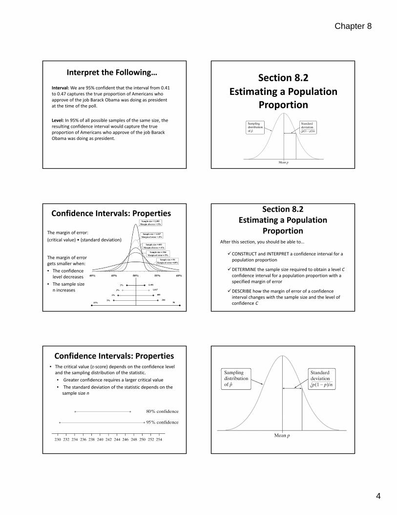
Confidence Intervals: Properties• The critical value (z‐score) depends on the confidence level
and the sampling distribution of the statistic.
• Greater confidence requires a larger critical value
• The standard deviation of the statistic depends on the sample size n
Section 8.2
Estimating a Population Proportion
Section 8.2Estimating a Population
ProportionAfter this section, you should be able to…
CONSTRUCT and INTERPRET a confidence interval for a population proportion
DETERMINE the sample size required to obtain a level Cconfidence interval for a population proportion with a specified margin of error
DESCRIBE how the margin of error of a confidence interval changes with the sample size and the level of confidence C
Chapter 8
5
Estimating p & Constructing a CI: Conditions
1) Random: The data should come from a well‐designed random sample or randomized experiment.
2) Normal: The sampling distribution of the statistic is approximately Normal. We can use the Normal approximation to the sampling distribution as long as np ≥ 10 and n(1 – p) ≥ 10. However, if we don’t know p, we can replace p with to check normality.
3) Independent: Individual observations are independent. When sampling without replacement, the sample size n should be no more than 10% of the population size N (the 10% condition).
Formula: Confidence Interval for p
CI Proportions:
The Process: Confidence Intervals
Parameter: p = true proportion….
Assess Conditions:Random: SRS or random assignment
Sample Size: be sure to show both np ≥ 10 and n(1 –p) ≥ 10, the formula plugged and a sentence stating the values are greater than 10, therefore normal. Independent: 10% rule
Name Interval: 1‐proportion z‐Interval
Interval: Use your calculator. “We are ____% confident
that the interval from ____ to ____ will capture the true proportion of (context)…”
Conclude in Context: Answer the question being asked.
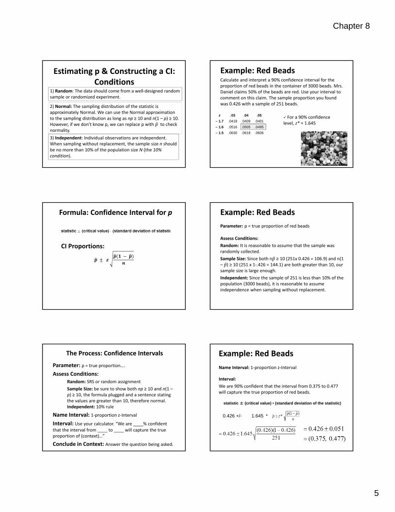
Example: Red BeadsCalculate and interpret a 90% confidence interval for the proportion of red beads in the container of 3000 beads. Mrs. Daniel claims 50% of the beads are red. Use your interval to comment on this claim. The sample proportion you found was 0.426 with a sample of 251 beads.
z .03 .04 .05
– 1.7 .0418 .0409 .0401
– 1.6 .0516 .0505 .0495
– 1.5 .0630 .0618 .0606
For a 90% confidence level, z* = 1.645
Example: Red Beads
Parameter: p = true proportion of red beads
Assess Conditions:
Random: It is reasonable to assume that the sample was randomly collected.
Sample Size: Since both n ≥ 10 (251x 0.426 = 106.9) and n(1 – ) ≥ 10 (251 x 1‐.426 = 144.1) are both greater than 10, our sample size is large enough.
Independent: Since the sample of 251 is less than 10% of the population (3000 beads), it is reasonable to assume independence when sampling without replacement.
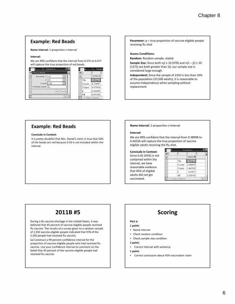
Example: Red Beads
Name Interval: 1‐proportion z‐Interval
Interval:
We are 90% confident that the interval from 0.375 to 0.477 will capture the true proportion of red beads.
statistic ± (critical value) • (standard deviation of the statistic)
0.426 +/- 1.645 *
Chapter 8
6
Example: Red Beads
Name Interval: 1‐proportion z‐Interval
Interval:
We are 90% confident that the interval from 0.375 to 0.477 will capture the true proportion of red beads.
Example: Red Beads
Conclude in Context:
It is pretty doubtful that Mrs. Daniel’s claim in true that 50% of the beads are red because 0.50 is not included within the interval.
2011B #5During a flu vaccine shortage in the United States, it was believed that 45 percent of vaccine‐eligible people received flu vaccine. The results of a survey given to a random sample of 2,350 vaccine‐eligible people indicated that 978 of the 2,350 people had received flu vaccine.
(a) Construct a 99 percent confidence interval for the proportion of vaccine‐eligible people who had received flu vaccine. Use your confidence interval to comment on the belief that 45 percent of the vaccine‐eligible people had received flu vaccine.
Parameter: p = true proportion of vaccine eligible people receiving flu shot
Assess Conditions:
Random: Random sample, stated.
Sample Size: Since both n ̂ ≥ 10 (978) and n(1 – ̂) ≥ 10 (1372) are both greater than 10, our sample size is considered large enough.
Independent: Since the sample of 2350 is less than 10% of the population (23,500 adults), it is reasonable to assume independence when sampling without replacement.
Name Interval: 1‐proportion z‐Interval
Interval:
We are 99% confident that the interval from 0.38998 to 0.44236 will capture the true proportion of vaccine eligible adults receiving the flu shot.
Conclude in Context: Since 0.45 (45%) is not contained within the interval, we have reasonable evidence that 45% of eligible adults did not get vaccinated.
ScoringPart a:
1 point:
• Name interval
• Check random condition
• Check sample size condition
1 point:
• Correct interval with sentence
1 point:
• Correct conclusion about 45% vaccination claim
Chapter 8
7
Calculating the Minimum Sample Size
In planning a study, we may want to choose a sample size that allows us to estimate a population proportion within a given margin of error by plugging in the desired margin of error (ME), the desired confidence level (z‐score) and the known to the margin of error formula. We then solve for n.
If the sample proportion is unknown we use = 0.5 as our best guess, because ME will be largest when = 0.5.
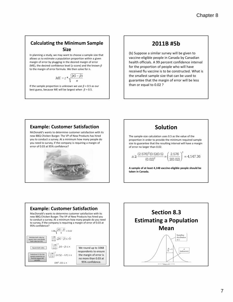
Example: Customer SatisfactionMcDonald's wants to determine customer satisfaction with its new BBQ Chicken Burger. The VP of New Products has hired you to conduct a survey. At a minimum how many people do you need to survey, if the company is requiring a margin of error of 0.03 at 95% confidence?
Example: Customer SatisfactionMacDonald's wants to determine customer satisfaction with its new BBQ Chicken Burger. The VP of New Products has hired you to conduct a survey. At a minimum how many people do you need to survey, if the company is requiring a margin of error of 0.03 at 95% confidence?
Multiply both sides by square root n and divide
both sides by 0.03.
Square both sides.
Substitute 0.5 for the sample proportion to find the largest ME
possible.
We round up to 1068 respondents to ensure the margin of error is no more than 0.03 at 95% confidence.
2011B #5b
(b) Suppose a similar survey will be given to vaccine‐eligible people in Canada by Canadian health officials. A 99 percent confidence interval for the proportion of people who will have received flu vaccine is to be constructed. What is the smallest sample size that can be used to guarantee that the margin of error will be less than or equal to 0.02 ?
SolutionThe sample‐size calculation uses 0.5 as the value of the proportion in order to provide the minimum required sample size to guarantee that the resulting interval will have a margin of error no larger than 0.02.
A sample of at least 4,148 vaccine‐eligible people should be taken in Canada.
Section 8.3
Estimating a Population Mean
Chapter 8
8
Section 8.3Estimating a Population Mean
After this section, you should be able to…
CONSTRUCT and INTERPRET a confidence interval for a population mean
DETERMINE the sample size required to obtain a level Cconfidence interval for a population mean with a specified margin of error
DESCRIBE how the margin of error of a confidence interval changes with the sample size and the level of confidence C
DETERMINE sample statistics from a confidence interval
Confidence Intervals: Conditions1) Random: The data should come from a well‐designed random sample or randomized experiment.
2) Normal: The sampling distribution of the statistic is approximately Normal. The sampling distribution is exactly Normal if the population distribution is Normal. When the population distribution is not Normal, then the central limit theorem tells us the sampling distribution will be approximately Normal if n is sufficiently large (n ≥ 30).
3) Independent: Individual observations are independent. When sampling without replacement, the sample size n should be no more than 10% of the population size N (the 10% condition).
Confidence Intervals: Formula
General Formula:point estimator z‐score standard deviation of the statistic
CI Means:
z ( )
Determining Minimum Sample Size
The margin of error ME of the confidence interval for the population mean µ is:
We determine a sample size for a desired margin of error when estimating a mean in much the same way we did when estimating a proportion.
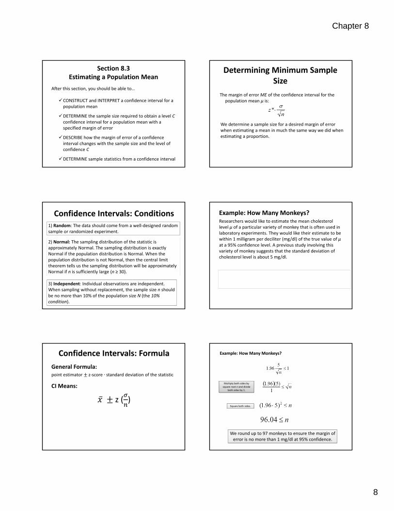
Example: How Many Monkeys?Researchers would like to estimate the mean cholesterol level µ of a particular variety of monkey that is often used in laboratory experiments. They would like their estimate to be within 1 milligram per deciliter (mg/dl) of the true value of µ at a 95% confidence level. A previous study involving this variety of monkey suggests that the standard deviation of cholesterol level is about 5 mg/dl.
The critical value for 95% confidence is z* = 1.96.
We will use σ = 5 as our best guess for the standard deviation.
Example: How Many Monkeys?
Multiply both sides by square root n and divide
both sides by 1.
Square both sides.
We round up to 97 monkeys to ensure the margin of error is no more than 1 mg/dl at 95% confidence.
Chapter 8
9
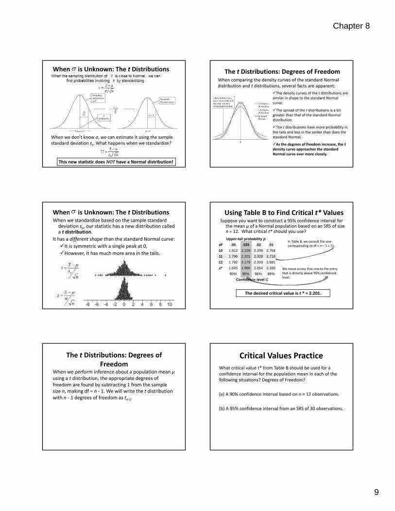
When is Unknown: The t Distributions
When we don’t know σ, we can estimate it using the sample standard deviation sx. What happens when we standardize?
This new statistic does NOT have a Normal distribution!
When is Unknown: The t DistributionsWhen we standardize based on the sample standard deviation sx, our statistic has a new distribution called a t distribution.
It has a different shape than the standard Normal curve:
It is symmetric with a single peak at 0,
However, it has much more area in the tails.
The t Distributions: Degrees of Freedom
When we perform inference about a population mean µ using a t distribution, the appropriate degrees of freedom are found by subtracting 1 from the sample size n, making df = n ‐ 1. We will write the t distribution with n ‐ 1 degrees of freedom as tn‐1.
The t Distributions: Degrees of FreedomWhen comparing the density curves of the standard Normal distribution and t distributions, several facts are apparent:
The density curves of the t distributions are similar in shape to the standard Normal curve.
The spread of the t distributions is a bit greater than that of the standard Normal distribution.
The t distributions have more probability in the tails and less in the center than does the standard Normal.
As the degrees of freedom increase, the t density curve approaches the standard Normal curve ever more closely.
Using Table B to Find Critical t* ValuesSuppose you want to construct a 95% confidence interval for
the mean µ of a Normal population based on an SRS of size n = 12. What critical t* should you use?
In Table B, we consult the row corresponding to df = n – 1 = 11.
The desired critical value is t * = 2.201.
We move across that row to the entry that is directly above 95% confidence level.
Upper-tail probability p
df .05 .025 .02 .01
10 1.812 2.228 2.359 2.764
11 1.796 2.201 2.328 2.718
12 1.782 2.179 2.303 2.681
z* 1.645 1.960 2.054 2.326
90% 95% 96% 98%
Confidence level C
Critical Values PracticeWhat critical value t* from Table B should be used for a confidence interval for the population mean in each of the following situations? Degrees of Freedom?
(a) A 90% confidence interval based on n = 12 observations.
(b) A 95% confidence interval from an SRS of 30 observations.
Chapter 8
10
Critical Values PracticeWhat critical value t* from Table B should be used for a confidence interval for the population mean in each of the following situations? Degrees of Freedom?
(a) A 90% confidence interval based on n = 12 observations.
df = 11, t*= 1.796
(b) A 95% confidence interval from an SRS of 30 observations.
df = 29, t*=2.045
The Process: Confidence Intervals
Parameter: = true mean….
Assess Conditions:Random: SRS or random assignment
Normal: DRAW boxplot, if sample is less than 30.
Independent: 10% rule
Name Interval: t‐Interval
Interval: Use your calculator. “We are ____% confident
that the interval from ____ to ____ will capture the true mean of (context)…”
Conclude in Context: Answer the question being asked.
t Distribution: Normal Condition
• Sample size less than 15: Use t procedures if the data appear close to Normal (roughly symmetric, single peak, no outliers). If the data are clearly skewed or if outliers are present, do not use t.
• Sample size at least 15: The t procedures can be used except in the presence of outliers or strong skewness.
• Large samples: The t procedures can be used even for clearly skewed distributions when the sample is large, roughly n ≥ 30.
Example: Milk Quality Control
A milk processor monitors the number of bacteria per milliliter in raw milk received at the factory. A random sample of 10 one‐milliliter specimens of milk supplied by one producer gives the following data:
Construct and interpret a 95% confidence interval for the population mean μ.
5370 4890 5100 4500 5260
5150 4900 4760 4700 4870
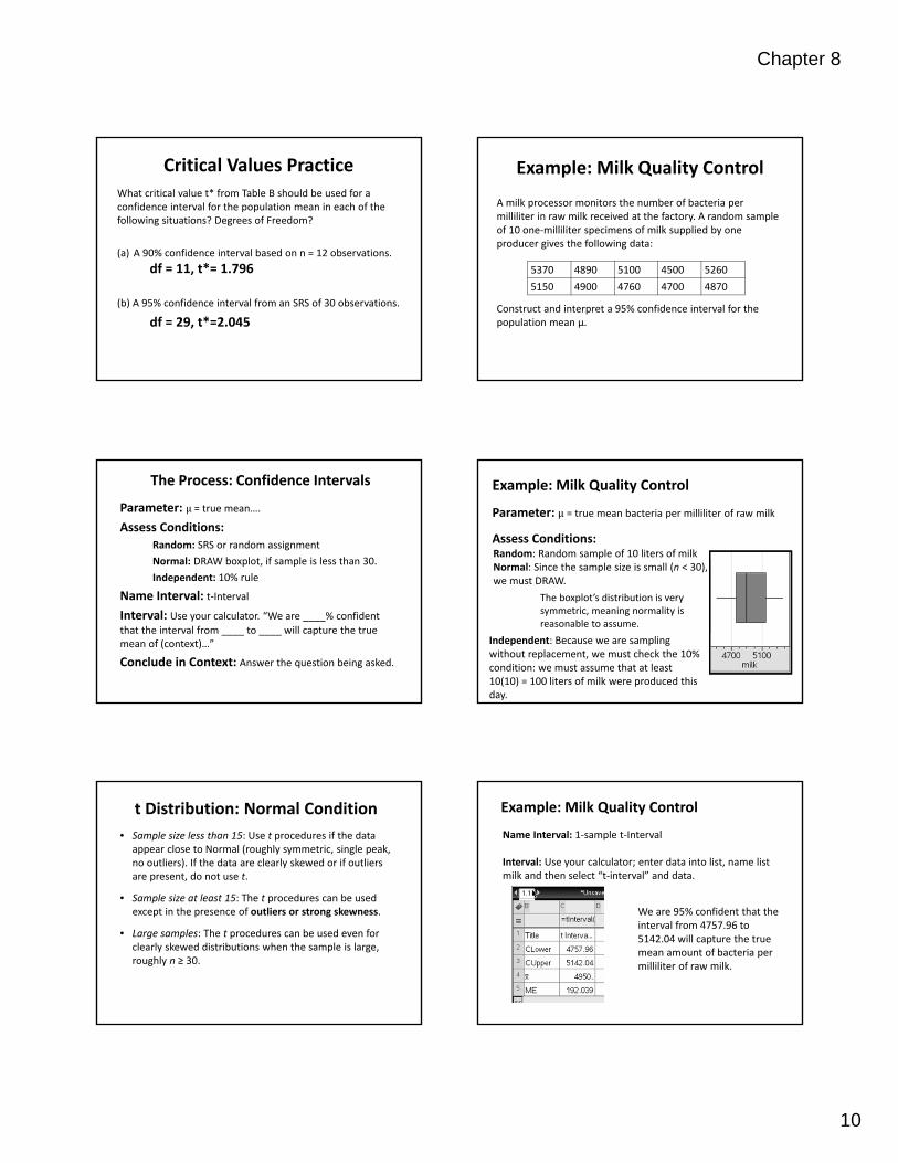
Example: Milk Quality Control
Parameter: = true mean bacteria per milliliter of raw milk
Assess Conditions:Random: Random sample of 10 liters of milkNormal: Since the sample size is small (n < 30), we must DRAW.
Independent: Because we are sampling without replacement, we must check the 10% condition: we must assume that at least 10(10) = 100 liters of milk were produced this day.
The boxplot’s distribution is very symmetric, meaning normality is reasonable to assume.
Example: Milk Quality Control
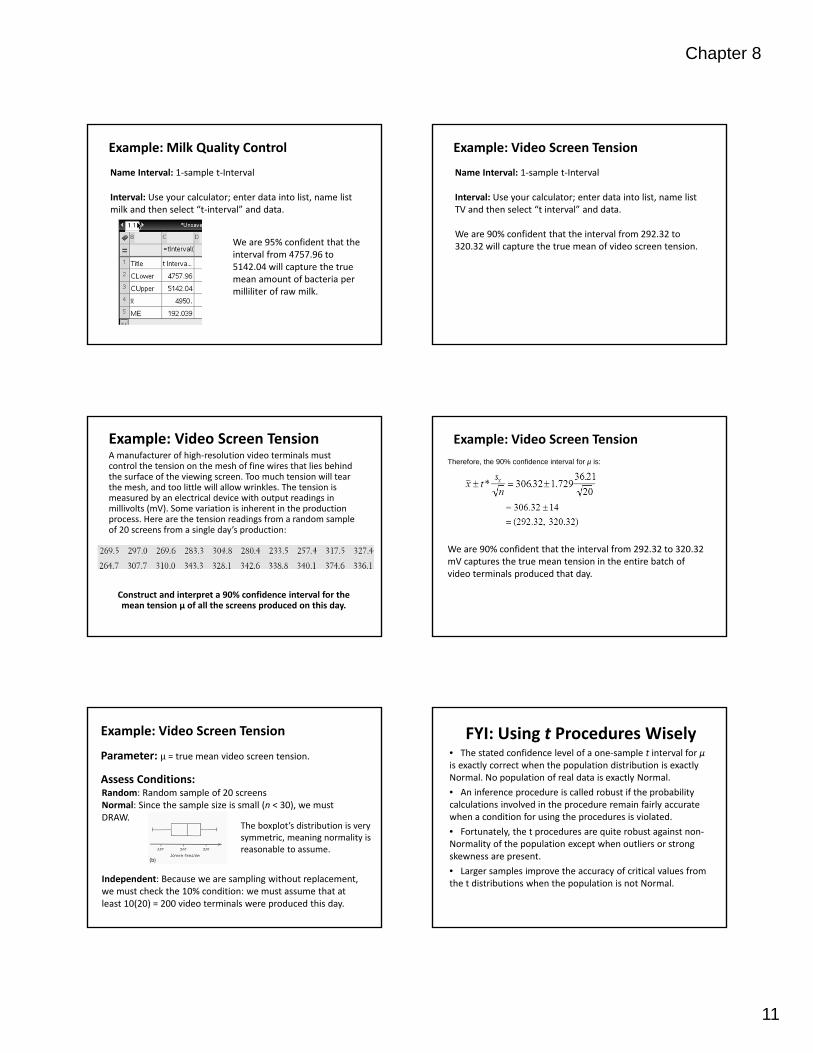
Name Interval: 1‐sample t‐Interval
Interval: Use your calculator; enter data into list, name list milk and then select “t‐interval” and data.
We are 95% confident that the interval from 4757.96 to 5142.04 will capture the true mean amount of bacteria per milliliter of raw milk.
Chapter 8
11
Example: Milk Quality Control
Name Interval: 1‐sample t‐Interval
Interval: Use your calculator; enter data into list, name list milk and then select “t‐interval” and data.
We are 95% confident that the interval from 4757.96 to 5142.04 will capture the true mean amount of bacteria per milliliter of raw milk.
Example: Video Screen TensionA manufacturer of high‐resolution video terminals must control the tension on the mesh of fine wires that lies behind the surface of the viewing screen. Too much tension will tear the mesh, and too little will allow wrinkles. The tension is measured by an electrical device with output readings in millivolts (mV). Some variation is inherent in the production process. Here are the tension readings from a random sample of 20 screens from a single day’s production:
Construct and interpret a 90% confidence interval for the mean tension μ of all the screens produced on this day.
Example: Video Screen Tension
Parameter: = true mean video screen tension.
Assess Conditions:Random: Random sample of 20 screensNormal: Since the sample size is small (n < 30), we must DRAW.
Independent: Because we are sampling without replacement, we must check the 10% condition: we must assume that at least 10(20) = 200 video terminals were produced this day.
The boxplot’s distribution is very symmetric, meaning normality is reasonable to assume.
Example: Video Screen Tension
Name Interval: 1‐sample t‐Interval
Interval: Use your calculator; enter data into list, name list TV and then select “t interval” and data.
We are 90% confident that the interval from 292.32 to 320.32 will capture the true mean of video screen tension.
Example: Video Screen Tension
We are 90% confident that the interval from 292.32 to 320.32 mV captures the true mean tension in the entire batch of video terminals produced that day.
Therefore, the 90% confidence interval for µ is:
FYI: Using t Procedures Wisely• The stated confidence level of a one‐sample t interval for µ is exactly correct when the population distribution is exactly Normal. No population of real data is exactly Normal.
• An inference procedure is called robust if the probability calculations involved in the procedure remain fairly accurate when a condition for using the procedures is violated.
• Fortunately, the t procedures are quite robust against non‐Normality of the population except when outliers or strong skewness are present.
• Larger samples improve the accuracy of critical values from the t distributions when the population is not Normal.
Chapter 8
12
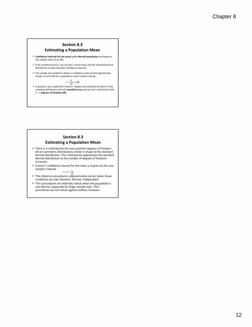
Section 8.3Estimating a Population Mean
Confidence intervals for the mean µ of a Normal population are based on the sample mean of an SRS.
If we somehow know σ, we use the z critical value and the standard Normal distribution to help calculate confidence intervals.
The sample size needed to obtain a confidence interval with approximate margin of error ME for a population mean involves solving
In practice, we usually don’t know σ. Replace the standard deviation of the sampling distribution with the standard error and use the t distribution with n – 1 degrees of freedom (df).
Section 8.3Estimating a Population Mean
There is a t distribution for every positive degrees of freedom. All are symmetric distributions similar in shape to the standard Normal distribution. The t distribution approaches the standard Normal distribution as the number of degrees of freedom increases.
A level C confidence interval for the mean µ is given by the one‐sample t interval
This inference procedure is approximately correct when these conditions are met: Random, Normal, Independent.
The t procedures are relatively robust when the population is non‐Normal, especially for larger sample sizes. The t procedures are not robust against outliers, however.