Interstellar Neutral Helium in the Heliosphere from IBEX Observations. V. Observationsin IBEX-Lo ESA Steps 1, 2, and 3

Paweł Swaczyna1 , Maciej Bzowski1 , Marzena A. Kubiak1, Justyna M. Sokół1, Stephen A. Fuselier2,3, André Galli4 ,David Heirtzler5, Harald Kucharek5, David J. McComas6 , Eberhard Möbius5 , Nathan A. Schwadron5 , and P. Wurz4

1 Space Research Centre of the Polish Academy of Sciences (CBK PAN), Bartycka 18A, 00-716 Warsaw, Poland; bzowski@cbk.waw.pl2 Southwest Research Institute, San Antonio, TX 78228, USA3 University of Texas at San Antonio, San Antonio, TX, USA4 Physics Institute, University of Bern, Bern, 3012, Switzerland

5 University of New Hampshire, Durham, NH 03824, USA6 Department of Astrophysical Sciences, Princeton University, Princeton, NJ 08544, USA

Received 2017 December 8; revised 2018 January 12; accepted 2018 January 28; published 2018 February 20

Abstract

Direct-sampling observations of interstellar neutral (ISN) He by the Interstellar Boundary Explorer (IBEX) providevaluable insight into the physical state of and processes operating in the interstellar medium ahead of theheliosphere. The ISN He atom signals are observed at the four lowest ESA steps of the IBEX-Lo sensor. Theobserved signal is a mixture of the primary and secondary components of ISN He and H. Previously, only datafrom one of the ESA steps have been used. Here, we extend the analysis to data collected in the three lowest ESAsteps with the strongest ISN He signal, for the observation seasons 2009–2015. The instrument sensitivity ismodeled as a linear function of the atom impact speed onto the sensor’s conversion surface separately for eachESA step of the instrument. We find that the sensitivity increases from lower to higher ESA steps, but within eachof the ESA steps it is a decreasing function of the atom impact speed. This result may be influenced by thehydrogen contribution, which was not included in the adopted model, but seems to exist in the signal. We concludethat the currently accepted temperature of ISN He and velocity of the Sun through the interstellar medium do notneed a revision, and we sketch a plan of further data analysis aiming at investigating ISN H and a betterunderstanding of the population of ISN He originating in the outer heliosheath.

Key words: instrumentation: detectors – ISM: atoms – ISM: kinematics and dynamics – local interstellar matter –methods: data analysis – Sun: heliosphere

1. Introduction

Direct sampling of interstellar neutral (ISN) gas in theheliosphere is a powerful tool for investigating the physicalstate of the interstellar matter ahead of the heliosphere (Möbiuset al. 2009). The ISN gas is a mixture of various elements,mostly hydrogen and helium (Frisch et al. 2011). Strongionization processes deplete the population of ISN H close tothe Sun and thus ISN He is the most abundant species at 1 au(Ruciński et al. 2003). Due to the long mean free path of theneutral He atoms in the interstellar medium most of theobserved ISN atoms are created in the unperturbed mediumwell ahead of the heliosphere (Bzowski et al. 2017). Theseatoms are collectively called the primary ISN population.Moreover, an additional population of atoms is created in theinterstellar medium modified due to interaction with theheliosphere—the secondary ISN population (Baranov &Malama 1995).

Results of in-depth analyses of direct-sampling observationsfrom GAS/Ulysses (Witte 2004; Bzowski et al. 2014; Woodet al. 2015) and from IBEX-Lo (Bzowski et al. 2015; McComaset al. 2015a, 2015b; Möbius et al. 2015a; Schwadron et al.2015) provided the direction, speed, and temperature of theprimary ISN He inflowing to the heliosphere. In addition tothe primary ISN He, IBEX-Lo discovered the Warm Breeze(Bzowski et al. 2012; Kubiak et al. 2014). This most likely isthe secondary population of ISN He, created via chargeexchange between interstellar He+ ions and ISN He atoms inthe outer heliosheath (Kubiak et al. 2016; Bzowski et al. 2017)and thus bears information on the plasma flow in the region

beyond the heliopause. The signal measured by IBEX-Locannot be easily separated into the primary and secondarycomponents. Moreover, due to the measurement techniqueused by IBEX-Lo (Möbius et al. 2009; Park et al. 2015), it ischallenging to uniquely identify the counts registered by theIBEX-Lo instrument due to neutral He and H atoms.Consequently, the signal observed by IBEX-Lo is a sum ofthe primary and secondary populations of ISN He and ISN H.ISN H has been identified in IBEX-Lo observations (Saul

et al. 2012, 2013; Schwadron et al. 2013), but the under-standing of the signal in different ESA steps of IBEX-Lo is stillnot satisfactory (Schwadron et al. 2013; Katushkinaet al. 2015). One of the reasons was an inaccurate knowledgeof the radiation pressure acting on H atoms in the heliosphere(Kowalska-Leszczynska et al. 2018). The ability to resolve theISN H and ISN He components in the observed signal isimportant because ISN H plays a vital role in generalheliospheric studies and because neglecting the hydrogencontribution in the He signal may bias the inferred parametersof inflow of interstellar matter on the heliosphere, as illustratedby the differences in the estimates of these parameters byBzowski et al. (2012) and Möbius et al. (2012) on one hand andby Bzowski et al. (2015), Leonard et al. (2015), Möbius et al.(2015a), and Schwadron et al. (2015) on the other. Adiscussion of this topic was provided by Swaczyna et al.(2015) and Bzowski et al. (2015).IBEX-Lo is a time-of-flight mass spectrometer (Fuselier et al.

2009) that measures neutral atoms by registering their negativeions, created upon impact on a specially prepared conversion

The Astrophysical Journal, 854:119 (13pp), 2018 February 20 https://doi.org/10.3847/1538-4357/aaabbf© 2018. The American Astronomical Society. All rights reserved.

1

surface. The conversion surface is permanently covered with athin layer of water, constantly replenished due to outgassing ofmaterial from the sensor and the spacecraft. Thus, in addition tonegative ions from the direct ionization mechanism, negativelycharged products of sputtering of material from the conversionsurface are registered (Wurz et al. 2006). In the case of Hatoms, the first mechanism dominates. However, He atomsrarely form negative ions (Wurz et al. 2008) and therefore theyare detected owing to the second mechanism. The productssputtered by He atoms from the water layer make the IBEX-Loinstrument sensitive to He atoms with energies typical for ISNatoms at 1 au from the Sun. The ions sputtered by He atomsfrom this water layer are primarily H− and O− ions. Thus, thesignal interpreted as coming from He atoms can originate bothfrom H− ions sputtered off the conversion surface by theincoming He atoms and from real H atoms reflected andionized on the conversion surface. Disentangling the twocontributions requires a detailed analysis (Park et al. 2016).Calibration of the sensitivity of IBEX-Lo to H atoms withvarious energies was carried out in the laboratory, but this waspossible only within certain limitations due to challenges inobtaining a monoenergetic beam of neutral atoms with relevantenergies (Wieser & Wurz 2005) and because the water layer onthe conversion surface may be different between the laboratoryand space conditions.

IBEX-Lo does not directly measure the energy of theimpacting atoms. It detects ions created at the conversionsurface with energies within the energy range set by theelectrostatic analyzer (ESA) and rejects those with the energiesoutside this preselected range. Ions with different energies areobserved when the instrument is switched to a different energysetting. The atoms directly converted to negative ions preservemost of their energies, but the ions sputtered from theconversion surface have a broad energy distribution, limitedby the energy of the impacting atoms. As discussed later in thepaper, ISN He is visible in the four lowest energy settings ofthe ESA (hereafter ESA steps), but so far only measurementsfrom ESA step 2 have been used in the analyses of ISN He. Inthis paper, we extend the analysis to ESA steps 1 and 3. ESAstep 4 is left out because of significantly lower count rates (by afactor of ∼5). A better insight into the physics of interaction ofthe heliosphere with interstellar matter could potentially beobtained if data from the three ESA steps with the highestcount rates are used. The factor that has been preventing the useof data from all of them is the lack of relative calibration of theESA steps for He atoms.

In the preliminary analyses (Möbius et al. 2009, 2012;Bzowski et al. 2012) it was assumed that the sensitivityfunction to various energies in ESA step 2 is flat, i.e., that thesensitivity is independent of energy. However, Kubiak et al.(2014), Sokół et al. (2015a), and Galli et al. (2015) showedevidence that, most likely, there is a threshold for the sensitivityto He atoms at an energy between 19 and 38eV. This is lowcompared to the ∼130 eV incident energy of the ISN He atoms.However, this threshold was shown to be particularly importantfor the analysis of the Warm Breeze (Kubiak et al. 2014, Figure8) and for the attempt to find ISN He in observations carriedout during the fall ISN observation seasons (Galli et al. 2015).

In this paper we make the first attempt to simultaneouslydetermine the inflow velocity vector, the temperature of ISNHe, and the relative energy sensitivity characteristics of theIBEX-Lo detector to He atoms using data from the three lowest

ESA steps. We use measurements from the ISN observationcampaigns 2009 through 2015, i.e., one season more than in theprevious analyses (Bzowski et al. 2015; Möbius et al. 2015a).First, we discuss the data, the adopted models, and the analysismethod (Section 2). Then, we present results of the analysis,including the relative energy sensitivity characteristics of thethree ESA steps of IBEX-Lo (Section 3). Finally, we discusssome implications of the findings (Section 4).

2. Methods

2.1. IBEX-Lo Observations

IBEX-Lo observations are carried out in eight partiallyoverlapping, logarithmically spaced, sequentially switchedenergy channels (the ESA steps). The full width at halfmaximum of the ESA steps is ΔE ; 0.7E, where E is thecentral energy of a given ESA step. For our purposes, the mostrelevant are the three lowest channels, i.e., ESA steps 1–3, withcentral energies 15, 29, and 55eV, respectively (Fuselier et al.2009, 2012). The absolute sensitivity of the instrument dependson the post-acceleration (PAC) voltage in the ESA. This valueis generally kept constant, but once during the mission, afterthe fourth ISN campaign, it was reduced. As discussed byBzowski et al. (2015), this resulted in an approximatelytwofold reduction in the absolute sensitivity to He atoms. Thecentral energies and widths of the ESA steps correspond toenergies of incident H atoms that are converted to negativeions. The energy loss is small in this situation. Helium atomsare observed due to the sputtering of material from theconversion surface. This process results in a significantly largerenergy difference between the incident He atom and thesputtered H− ion. The sputtered ions have a wide energyspectrum and are observed in the ESA steps with centralenergies much below the energies of the incident ISN Heatoms.Details of the operation of the IBEX-Lo instrument during

the yearly campaigns of observations of ISN gas have beenextensively presented in the literature (e.g., Bzowski et al.2015; Möbius et al. 2015b) and will not be repeated here. Inbrief, IBEX is a spin-stabilized Earth satellite in a veryelongated orbit (McComas et al. 2009). To maintain the spinaxis within a few degrees from the Sun, it was adjusted onceper orbit during the first three years of operation, and isadjusted twice per orbit after the IBEX orbit change in 2011(McComas et al. 2011). The boresight of IBEX-Lo pointsperpendicular to the spin axis. For a given orientation of thespin axis, data are collected from the great circle of the skyvisible to the instrument for several days when the spacecraft issufficiently high above the magnetopause. The registeredcounts are binned into 6° spin angle bins.On the ground, the data are filtered against all known

perturbations. Due to this filtering, some intervals of theobservations are excluded. The intervals used in the analysisare referred to as ISN good times. In this paper, the previouslyused ISN good times (Leonard et al. 2015; Möbius et al.2015b) are further restricted by adopting the intervals includedin the good times obtained from an in-depth investigation of thesources of background and foreground, presented by Galli et al.(2015, 2016, 2017). This restriction results in shorteraccumulation times in several orbits and rejection of all datafrom orbit 237b. The list of orbits selected for this analysis ispresented in Table 1. The background level was also revised

2

The Astrophysical Journal, 854:119 (13pp), 2018 February 20 Swaczyna et al.

following results from Galli et al. (2016, 2017). The data subsetused now is cleaner, which results in a slightly lower χ2

obtained in the present fitting than that by Bzowski et al. (2015)as will be evident from the results presented below.

The data used in this analysis include (1) intervals of thegood times and (2) the numbers of counts due to ISN atoms,collected during these time intervals in each individual 6° spinangle bin. From this information, we calculate mean countingrates for each bin for a given orbit.

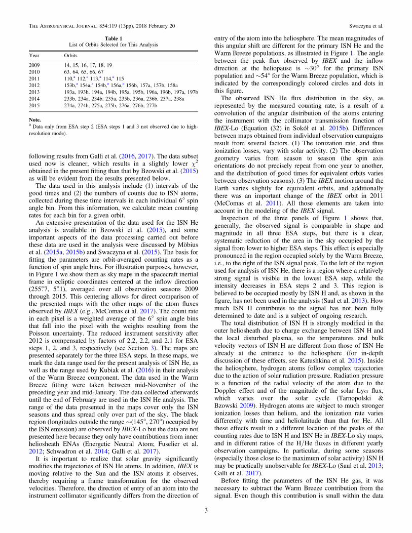
An extensive presentation of the data used for the ISN Heanalysis is available in Bzowski et al. (2015), and someimportant aspects of the data processing carried out beforethese data are used in the analysis were discussed by Möbiuset al. (2015a, 2015b) and Swaczyna et al. (2015). The basis forfitting the parameters are orbit-averaged counting rates as afunction of spin angle bins. For illustration purposes, however,in Figure 1 we show them as sky maps in the spacecraft inertialframe in ecliptic coordinates centered at the inflow direction(255°.7, 5°.1), averaged over all observation seasons 2009through 2015. This centering allows for direct comparison ofthe presented maps with the other maps of the atom fluxesobserved by IBEX (e.g., McComas et al. 2017). The count ratein each pixel is a weighted average of the 6° spin angle binsthat fall into the pixel with the weights resulting from thePoisson uncertainty. The reduced instrument sensitivity after2012 is compensated by factors of 2.2, 2.2, and 2.1 for ESAsteps 1, 2, and 3, respectively (see Section 3). The maps arepresented separately for the three ESA steps. In these maps, wemark the data range used for the present analysis of ISN He, aswell as the range used by Kubiak et al. (2016) in their analysisof the Warm Breeze component. The data used in the WarmBreeze fitting were taken between mid-November of thepreceding year and mid-January. The data collected afterwardsuntil the end of February are used in the ISN He analysis. Therange of the data presented in the maps cover only the ISNseasons and thus spread only over part of the sky. The blackregion (longitudes outside the range ∼(145°, 270°) occupied bythe ISN emission) are observed by IBEX-Lo but the data are notpresented here because they only have contributions from innerheliosheath ENAs (Energetic Neutral Atom; Fuselier et al.2012; Schwadron et al. 2014; Galli et al. 2017).

It is important to realize that solar gravity significantlymodifies the trajectories of ISN He atoms. In addition, IBEX ismoving relative to the Sun and the ISN atoms it observes,thereby requiring a frame transformation for the observedvelocities. Therefore, the direction of entry of an atom into theinstrument collimator significantly differs from the direction of

entry of the atom into the heliosphere. The mean magnitudes ofthis angular shift are different for the primary ISN He and theWarm Breeze populations, as illustrated in Figure 1. The anglebetween the peak flux observed by IBEX and the inflowdirection at the heliopause is ∼30° for the primary ISNpopulation and ∼54° for the Warm Breeze population, which isindicated by the correspondingly colored circles and dots inthis figure.The observed ISN He flux distribution in the sky, as

represented by the measured counting rate, is a result of aconvolution of the angular distribution of the atoms enteringthe instrument with the collimator transmission function ofIBEX-Lo (Equation (32) in Sokół et al. 2015b). Differencesbetween maps obtained from individual observation campaignsresult from several factors. (1) The ionization rate, and thusionization losses, vary with solar activity. (2) The observationgeometry varies from season to season (the spin axisorientations do not precisely repeat from one year to another,and the distribution of good times for equivalent orbits variesbetween observation seasons). (3) The IBEX motion around theEarth varies slightly for equivalent orbits, and additionallythere was an important change of the IBEX orbit in 2011(McComas et al. 2011). All those elements are taken intoaccount in the modeling of the IBEX signal.Inspection of the three panels of Figure 1 shows that,

generally, the observed signal is comparable in shape andmagnitude in all three ESA steps, but there is a clear,systematic reduction of the area in the sky occupied by thesignal from lower to higher ESA steps. This effect is especiallypronounced in the region occupied solely by the Warm Breeze,i.e., to the right of the ISN signal peak. To the left of the regionused for analysis of ISN He, there is a region where a relativelystrong signal is visible in the lowest ESA step, while theintensity decreases in ESA steps 2 and 3. This region isbelieved to be occupied mostly by ISN H and, as shown in thefigure, has not been used in the analysis (Saul et al. 2013). Howmuch ISN H contributes to the signal has not been fullydetermined to date and is a subject of ongoing research.The total distribution of ISN H is strongly modified in the

outer heliosheath due to charge exchange between ISN H andthe local disturbed plasma, so the temperatures and bulkvelocity vectors of ISN H are different from those of ISN Healready at the entrance to the heliosphere (for in-depthdiscussion of these effects, see Katushkina et al. 2015). Insidethe heliosphere, hydrogen atoms follow complex trajectoriesdue to the action of solar radiation pressure. Radiation pressureis a function of the radial velocity of the atom due to theDoppler effect and of the magnitude of the solar Lyα flux,which varies over the solar cycle (Tarnopolski &Bzowski 2009). Hydrogen atoms are subject to much strongerionization losses than helium, and the ionization rate variesdifferently with time and heliolatitude than that for He. Allthese effects result in a different location of the peaks of thecounting rates due to ISN H and ISN He in IBEX-Lo sky maps,and in different ratios of the H/He fluxes in different yearlyobservation campaigns. In particular, during some seasons(especially those close to the maximum of solar activity) ISN Hmay be practically unobservable for IBEX-Lo (Saul et al. 2013;Galli et al. 2017).Before fitting the parameters of the ISN He gas, it was

necessary to subtract the Warm Breeze contribution from thesignal. Even though this contribution is small within the data

Table 1List of Orbits Selected for This Analysis

Year Orbits

2009 14, 15, 16, 17, 18, 192010 63, 64, 65, 66, 672011 110,a 112,a 113,a 114,a 1152012 153b,a 154a,a 154b,a 156a,a 156b, 157a, 157b, 158a2013 193a, 193b, 194a, 194b, 195a, 195b, 196a, 196b, 197a, 197b2014 233b, 234a, 234b, 235a, 235b, 236a, 236b, 237a, 238a2015 274a, 274b, 275a, 275b, 276a, 276b, 277b

Note.a Data only from ESA step 2 (ESA steps 1 and 3 not observed due to high-resolution mode).

3

The Astrophysical Journal, 854:119 (13pp), 2018 February 20 Swaczyna et al.

Figure 1. Sky maps of the count rate in s−1 due to ISN atoms observed by IBEX-Lo in ESA steps 1 (top), 2 (middle), and 3 (bottom) in the J2000 ecliptic coordinatescentered at the nose direction in the IBEX-inertial frame, averaged over the ISN campaigns 2009 through 2015 (the sensitivity decrease after 2012 is compensated for;see the text). The yellow and white dashed rectangles on the celestial sphere mark the data range used in the fitting of the primary ISN He in Bzowski et al. (2015) aswell as in the present paper, and in the fitting of the Warm Breeze in Kubiak et al. (2016), respectively. The solid contours mark where the contribution of the primaryISN He (yellow) and the Warm Breeze (white) signal in ESA step 2 is ≈0.1s−1; note that these contours are identical in all three panels to facilitate viewing thedifferences between the flux observed in the three ESA steps. The maxima of the two components (marked with open yellow and white circles) fall inside theirrespective contours. The dashed green line is the deflection plane of the secondary population as obtained by Kubiak et al. (2016). The unperturbed inflow directionsof these two populations are shown as the solid yellow and white dots on this plane. The red circle represents the center of the IBEX ribbon (Funsten et al. 2013) andthe red dot is the direction of the unperturbed interstellar magnetic field, derived by Zirnstein et al. (2016) from global models of the heliosphere using the geometry ofthe ribbon as constraints.

4

The Astrophysical Journal, 854:119 (13pp), 2018 February 20 Swaczyna et al.

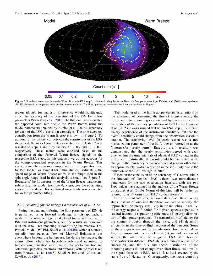
region adopted for analysis its presence would significantlyaffect the accuracy of the derivation of the ISN He inflowparameters (Swaczyna et al. 2015). To that end, we calculatedthe expected count rate due to the Warm Breeze using themodel parameters obtained by Kubiak et al. (2016), separatelyfor each of the ISN observation campaigns. The time-averagedcontribution from the Warm Breeze is shown in Figure 2. Toaccount for the differences between the sensitivities in the ESAsteps used, the model count rate calculated for ESA step 2 wasrescaled to steps 1 and 3 by factors 0.8±0.2 and 1.0±0.3,respectively. These factors were assessed based on thecomparison of the observed Warm Breeze signals in therespective ESA steps. In this analysis we do not account forthe energy-dependent response in the Warm Breeze. Thisvariation may be even more important for this population thanfor ISN He but we leave it for future studies. Fortunately, thespeed range of Warm Breeze atoms in the range used in thespin angle range used in this analysis is small (see Figure 3).Because of the fit uncertainty of the Warm Breeze parameters,subtracting this model from the data modifies the uncertaintysystem of the data. This additional uncertainty was accountedfor in the parameter fitting.

2.2. Accounting for the Energy Characteristics of IBEX-Lo

Fitting the data and inferring the flow parameters of ISN Heis performed using forward modeling. In this approach, amodel of the observed gas is calculated for an assumed set ofISN and instrument parameters, and the results are comparedwith the data. This modeling is done using the Warsaw TestParticle Model (WTPM, Sokół et al. 2015b), which assumes aspatially homogeneous flow of Maxwell–Boltzmann gaseverywhere beyond the heliopause. Inside the heliopause, theatoms follow heliocentric hyperbolic orbits and are subject totime-varying ionization losses due to solar photoionization andsolar wind particles (electrons and protons), with the rates takenfrom Bzowski et al. (2013), Sokół & Bzowski (2014), andSokół et al. (2016).

The model used in the fitting adopts certain assumptions onthe efficiency of converting the flux of atoms entering theinstrument into a counting rate returned by this instrument. Inthe studies of the primary population of ISN He by Bzowskiet al. (2015) it was assumed that within ESA step 2 there is noenergy dependence of the instrument sensitivity, but that theoverall sensitivity could change from one observation season toanother. The sensitivity level for each season was a freenormalization parameter of the fit, further on referred to as theY-norm (for “yearly norm”). Based on the fit results it wasdemonstrated that the yearly sensitivities agreed with eachother within the time intervals of identical PAC voltage in theinstrument. Statistically, this result could be interpreted as nochange in the sensitivity between individual seasons other thanan approximately twofold reduction in the sensitivity due to thereduction of the PAC voltage in 2012.Based on the conclusion of the constancy of Y-norms within

the intervals of identical PAC values, two normalizationparameters for the two observation intervals with the twoPAC values were adopted in the analysis of the Warm Breezeby Kubiak et al. (2016). Norms of this kind will be further onreferred to as P-norms (for “PAC voltage norms”).In the present analysis, we used data from three energy

steps instead of one and therefore we had to modify theapproach to the energy sensitivity in the modeling. In reality,the energy response function for a given species depends onseveral factors: (1) sputtering efficiency, (2) energy distribu-tion of the sputter products, (3) transmission efficiency forthe sputter products through the ESA, and (4) detectionefficiency in the time-of-flight section of the detector. Someof these aspects are not fully understood for the actual in-flight environment. Factors (1) and (2) are independent ofsetting the instrument to a given ESA step becauseobservations in different ESA steps are carried out in closesuccession, and the flux and speed distribution of theincoming atoms do not change over short times. As a result,the signal observed in ESA steps 1, 2, and 3 is created by thesame flux of He atoms. Consequently, the mean counting

Figure 2. Simulated count rate due to the Warm Breeze in ESA step 2, calculated using the Warm Breeze inflow parameters from Kubiak et al. (2016), averaged overall ISN observation campaigns used in the present analysis. The lines, points, and contours are identical to those in Figure 1.

5

The Astrophysical Journal, 854:119 (13pp), 2018 February 20 Swaczyna et al.

rates obtained in a given spin angle bin in a given IBEX orbitin these ESA steps differ solely due to the differentsensitivities of the instrument in these ESA steps (excludingthe inevitable statistical scatter).

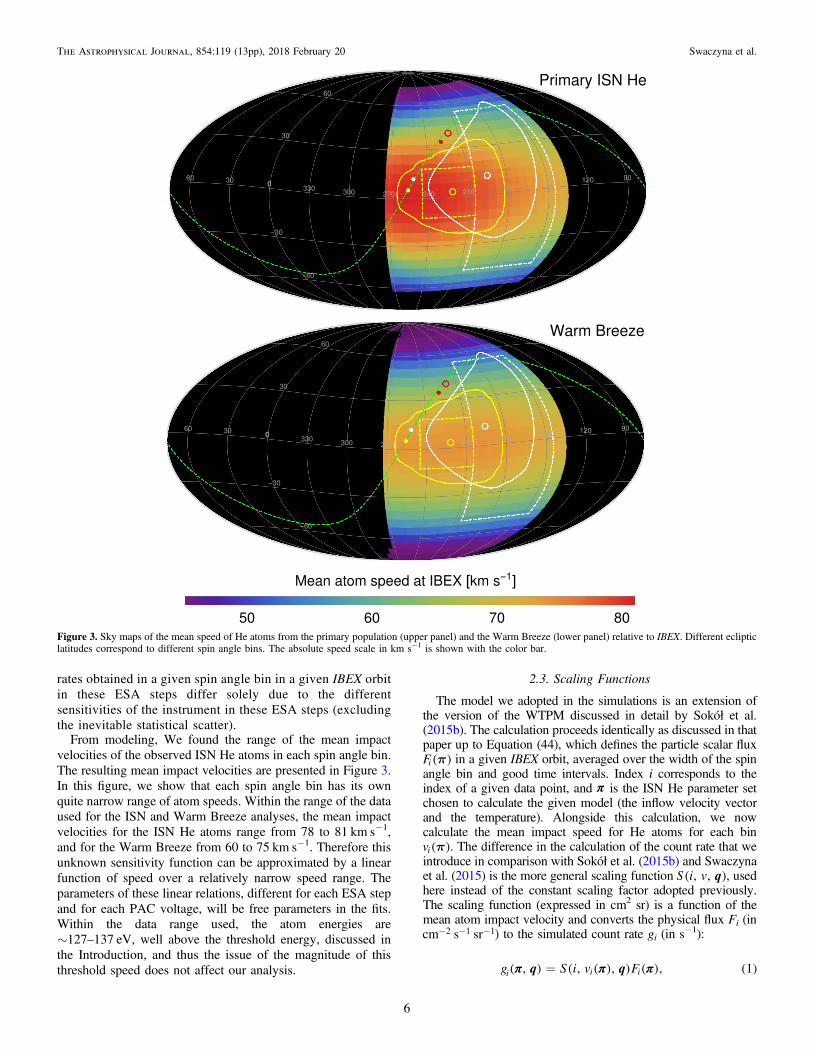
From modeling, We found the range of the mean impactvelocities of the observed ISN He atoms in each spin angle bin.The resulting mean impact velocities are presented in Figure 3.In this figure, we show that each spin angle bin has its ownquite narrow range of atom speeds. Within the range of the dataused for the ISN and Warm Breeze analyses, the mean impactvelocities for the ISN He atoms range from 78 to 81 km s−1,and for the Warm Breeze from 60 to 75 km s−1. Therefore thisunknown sensitivity function can be approximated by a linearfunction of speed over a relatively narrow speed range. Theparameters of these linear relations, different for each ESA stepand for each PAC voltage, will be free parameters in the fits.Within the data range used, the atom energies are∼127–137 eV, well above the threshold energy, discussed inthe Introduction, and thus the issue of the magnitude of thisthreshold speed does not affect our analysis.

2.3. Scaling Functions

The model we adopted in the simulations is an extension ofthe version of the WTPM discussed in detail by Sokół et al.(2015b). The calculation proceeds identically as discussed in thatpaper up to Equation (44), which defines the particle scalar fluxFi p( ) in a given IBEX orbit, averaged over the width of the spinangle bin and good time intervals. Index i corresponds to theindex of a given data point, and π is the ISN He parameter setchosen to calculate the given model (the inflow velocity vectorand the temperature). Alongside this calculation, we nowcalculate the mean impact speed for He atoms for each binvi p( ). The difference in the calculation of the count rate that weintroduce in comparison with Sokół et al. (2015b) and Swaczynaet al. (2015) is the more general scaling function qS i v, ,( ), usedhere instead of the constant scaling factor adopted previously.The scaling function (expressed in cm2 sr) is a function of themean atom impact velocity and converts the physical flux Fi (incm s sr2 1 1- - - ) to the simulated count rate gi (in s−1):

q qg S i v F, , , , 1i i i=π π π( ) ( ( ) ) ( ) ( )

Figure 3. Sky maps of the mean speed of He atoms from the primary population (upper panel) and the Warm Breeze (lower panel) relative to IBEX. Different eclipticlatitudes correspond to different spin angle bins. The absolute speed scale in kms−1 is shown with the color bar.

6

The Astrophysical Journal, 854:119 (13pp), 2018 February 20 Swaczyna et al.

where vi is the characteristic speed for a given orbit and spinangle bin, which is now calculated alongside Fi, and q is avector of parameters that define the scaling function.Importantly, Fi is a physical characteristic of the atomsobserved in this spin angle bin and orbit, which of coursedoes not depend on the ESA step of the instrument. In additionto Fi, the model now returns the average speed and the averagesquared speed for each bin.

The count rate calculation in Sokół et al. (2015b) was carriedour using the scaling function that is constant for each ISNseason:

S i v a a a a, , , , , , 2y iY 2009 2010 2014¼ =( { }) ( )( )

where y(i) give the years that represent each of the ISN seasons.This form represents Y-norms and means that the scalingfunction does not depend on the atom impact speed. Inclusionof more ESA steps would require three separate constants foreach ESA step and each ISN season. However, we verified thatthis is not necessary because the norms for individual seasonsare constant within two periods: before and after the decreaseof the PAC voltage. Consequently, we define the P-normsusing the scaling function in the form:

S i v a a, , , 3p e p e p i e iP ,ESA H,L; 1,2,3 ,ESA== =( { } ) ( )( ) ( )

where p(i) gives H or L for high/low PAC voltage, dependingif a given data point i was obtained before or after the decreaseof the PAC voltage, and e(i) gives the ESA step. Using theapproach with P-norms implies that a different parameter a isallowed for each energy step and the PAC voltage. As a result,for three energy steps the vector q of the parameters of functionSP has six elements.

If one allows for a true dependence of the sensitivity of theinstrument within a given ESA step on the atom speed, then thesimplest possible form of the scaling function is the linearfunction SPV, defined as:

S i v a b

a b v v

, , ,

1 , 4p e p e p e

p i e i p i e i

PV ,ESA ,ESA H,L; 1,2,3

,ESA ,ESA 0= + -= =( { } )

( ( )) ( )( ) ( ) ( ) ( )

where v0 is a certain reference speed, adopted here at78kms−1. This arbitrary choice does not affect the generalityof the scaling function because it only requires a simpletransformation for the parameters ap e,ESA for a different choiceof v0. The function SPV may be regarded as an expansion of anunknown true sensitivity function into a Taylor series, cut off atthe linear term. The parameters bp e,ESA are the relative changeof the absolute sensitivity per kms−1. In general one mayintroduce a function SYV defined in analogy to SPV but with theparameters depending on the season, and not the H/L PACvoltage.

2.4. Parameter Fitting

Parameter fitting is carried out using the method suggestedby Swaczyna et al. (2015) and successfully applied by Bzowskiet al. (2015) to obtain the inflow parameters of ISN He and byKubiak et al. (2016) to obtain the inflow parameters of theWarm Breeze. Swaczyna et al. (2015) discuss at length all datacorrelations that must be taken into account and we will notrepeat all those details. We only briefly recall that the modelmust be calculated on a regular parameter grid and that one

must compute the uncertainty covariance matrix V . With thoseon hand, we calculated the measure of goodness of fit given byχ2 defined as:

q q V qc g c g, , , 5i j

i i i j j j2

,

1,åp p pc = - --( ) ( ( ))( ) ( ( )) ( )

where i, j go over all data points used in the analysis, for allthree ESA steps, ci is the corrected count rate with the back-ground and Warm Breeze contribution subtracted (Swaczynaet al. 2015), and gi is calculated from Equation (1) with theS functions given by Equations (2)–(4). The fit parameters arep and q. The parameters p correspond to the sought ISNparameters (the magnitude and ecliptic coordinates of theinflow velocity, and the temperature), and the parameters qare the unknown parameters of the sensitivity function S. Thecalculation was performed on sets of the ISN He parameterstaken from a grid spaced at Δλ=1°, Δβ=0°.1, Δv=0.2 km s−1, v 0.1 km st

1D = - , with 4607 nodes around theISN He parameter values obtained by Bzowski et al. (2015).The optimum parameter set was found in a two-step process.

The first step was finding the parameter set q,p( ) with theminimum χ2 value calculated from Equation (5), evaluated forthose 4607 parameter sets. Subsequently, a quadratic form inthe parameter space was fitted to the χ2 surface near theintermediate minimum, and the parameter values for theabsolute minimum of this surface were calculated analytically.This resulted in a better parameter resolution than that obtaineddirectly from the parameter grid spacing. The fitting procedureis repeated for each considered data set and scaling functionform. Consequently, both the inflow parameters and theparameters q vary accordingly.Statistically, the expected value of min

2c is given byN N2min

2dof dofc , where Ndof is the number of degrees

of freedom. For Ndof we adopted the number of data pointsminus the number of fit parameters, similarly to Swaczyna et al.(2015), Bzowski et al. (2015), and Kubiak et al. (2016), eventhough this is strictly exact only for linear models, and ourmodel is nonlinear. Finally, the uncertainties of the soughtparameters are obtained from the curvature of the function

q,2 pc ( ) scaled using the scaling factor S N2dofc= as

presented in Swaczyna et al. (2015) and Bzowski et al. (2015).The parameters q,p( ) are correlated with each other, asdiscussed in Swaczyna et al. (2015).

3. Results

We began the parameter evaluation by repeating the analysisof Bzowski et al. (2015). We used a slightly more restrictivegood times list and slightly modified levels of the ubiquitousbackground (Galli et al. 2016, 2017). The contribution from theWarm Breeze was estimated from WTPM using the WarmBreeze parameters from Kubiak et al. (2016), i.e., differentfrom the Warm Breeze estimate used by Bzowski et al. (2015).This contribution was subtracted from the data and the relateduncertainty added to the uncertainty system. We performed fitsassuming Y-norms and using data from observation seasons2009–2014 and ESA step 2 only. The ISN He fit parameters arepresented in row 1 in Table 2, and the corresponding Y-normsin Table 3. In rows 0 of these tables the parameters found byBzowski et al. (2015) are presented for comparison. Weconclude that the new data selection, as well as the new Warm

7

The Astrophysical Journal, 854:119 (13pp), 2018 February 20 Swaczyna et al.

Breeze subtraction, does not substantially affect the ISN Heinflow parameters. The differences are small, well withinthe uncertainties. The largest discrepancy is in the temperature(∼250 K), and this is likely caused by the new WarmBreeze model subtracted here. The temperature of the WarmBreeze was found significantly lower by Kubiak et al. (2016)than obtained from the earlier analysis by Kubiak et al. (2014).Bzowski et al. (2015) adopted the higher temperature of theWarm Breeze from Kubiak et al. (2014). Consequently, aftersubtraction of the Warm Breeze in their analysis, the datafeatured a narrower peak, which the fitting procedureinterpreted as due to a lower temperature of ISN He. Thereduced χ2 value that we have obtained now, equal to N2

dofc ,is significantly lower than that obtained by Bzowski et al.(2015), i.e., the model better fits the data than in Bzowskiet al. (2015).

In the next step, we added the data from season 2015 to theanalysis (row 2). The resulting parameters remain almost thesame. Inspection of Table 3 shows that the obtained parametersof the scaling function are constant for the seasons with the HPAC voltage and separately with the L PAC voltage. Thevariation of these parameters is reduced by an order ofmagnitude with respect to that obtained by Bzowski et al.(2015). Moreover, the new values agree in these two periods,and the usage of the P-norms rather than Y-norms is justified.Results for the P-norms applied to ESA step 2 solely arepresented in row 3 of Tables 2 and 4. The obtained values ofthe norms agree with the values formerly found for eachseason. The ISN flow parameters are slightly different, but wellwithin the uncertainty ranges.

We found that including data from the 2016 campaignsignificantly increases the value of the reduced χ2. During thisseason, only data from three orbits before the absolute

maximum of ISN He count rate could be obtained due to atemporary issue with the IBEX star tracker system, whichmakes the data coverage for this campaign significantly poorer.Therefore, we decided to not include the data from this seasonin this analysis.Next, we checked how the fit parameter values change when

a variation of the instrument sensitivity with atom speed isallowed for, while continuing to use data solely from ESA step2. We used the function SPV from Equation (4) and list theresults in row 4 of Table 2. This modification resulted in asignificant reduction of the reduced χ2 value. The inflowlatitude and speed changed appreciably but within theuncertainty range.Subsequently, we tested whether including additional ESA

steps while assuming no dependence of the instrumentsensitivity to atom speed within individual ESA step returnssimilar results to those obtained by Bzowski et al. (2015), usingagain the sensitivity function SP. Finally, we allowed for thesensitivity within an ESA step to vary with atom speed whilecontinuing to use data from three ESA steps. To that end, wetook PV-norms and adopted the sensitivity function SPV fromEquation (4). The resulting ISN He parameters are presented inrows 5–8 of Table 2, and the norms in Table 4. As a result ofthese fittings we found that the ISN flow parameters aresubstantially different if all three ESA steps are included (rows7 and 8) from those obtained solely for ESA step 2, especiallyfor the inflow longitude. This effect is not present if ESA step 1is excluded (rows 5 and 6). The simultaneous increase in thereduced χ2 value for the three ESA steps suggests that themodel fit is significantly poorer. This is likely due to acontribution from ISN H, unaccounted for in the model. Weconsider this hypothesis is likely because eliminating ESA step1 from the data and fitting to data from ESA steps 2 and 3

Table 2ISN He Flow Parameters

Norm ESA Seasons λ(°) β(°) v (km s−1) T (K) M Ndof N

2

dof

c

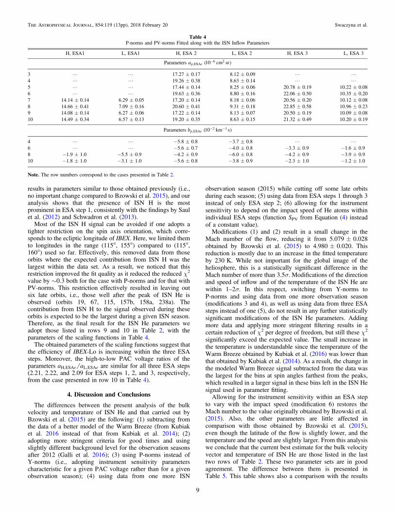
0a Y-norm 2 2009–2014 255.74±0.45 5.16±0.10 25.76±0.37 7440±260 5.079±0.028 254 1.841 Y-norm 2 2009–2014 255.70±0.47 5.14±0.11 25.71±0.43 7696±294 4.980±0.020 248 1.602 Y-norm 2 2009–2015 255.68±0.46 5.09±0.11 25.65±0.39 7677±285 4.976±0.019 289 1.553 P-norm 2 2009–2015 255.46±0.45 5.11±0.11 25.85±0.40 7805±278 4.972±0.019 294 1.614 PV-norm 2 2009–2015 255.48±0.46 4.91±0.09 26.23±0.42 7726±269 5.072±0.025 292 1.425 P-norm 2–3 2009–2015 254.76±0.33 5.20±0.08 26.49±0.30 8111±211 4.999±0.015 544 1.656 PV-norm 2–3 2009–2015 254.90±0.36 5.04±0.08 26.66±0.33 7938±208 5.085±0.019 540 1.457 P-norm 1–3 2009–2015 254.63±0.35 5.23±0.07 25.98±0.29 7853±208 4.982±0.016 794 1.978 PV-norm 1–3 2009–2015 253.82±0.37 5.06±0.07 26.98±0.33 8155±215 5.077±0.020 788 1.749 P-norm 1–3 2009–2015b 255.62±0.36 5.16±0.08 25.82±0.33 7673±225 5.010±0.015 686 1.6410 PV-norm 1–3 2009–2015b 255.41±0.40 5.03±0.07 26.21±0.37 7691±230 5.080±0.019 680 1.49

Notes.a Results from Bzowski et al. (2015).b Data range restricted to longitudes within 115°–155° (see the text).

Table 3Y-norms Fitted along with the ISN Inflow Parameters (ay,ESA2, 10 cm sr6 2- )

2009 2010 2011 2012 2013 2014 2015

0a 16.76 16.66 15.11 14.50 7.709 7.977 L1 17.18±0.19 17.08±0.20 17.47±0.28 17.27±0.22 8.03±0.10 8.25±0.10 L2 17.16±0.19 17.07±0.20 17.45±0.28 17.25±0.22 8.02±0.09 8.25±0.10 8.28±0.09

Note. The row numbers correspond to the cases presented in Table 2.a Results from Bzowski et al. (2015).

8

The Astrophysical Journal, 854:119 (13pp), 2018 February 20 Swaczyna et al.

results in parameters similar to those obtained previously (i.e.,no important change compared to Bzowski et al. 2015), and ouranalysis shows that the presence of ISN H is the mostprominent in ESA step 1, consistently with the findings by Saulet al. (2012) and Schwadron et al. (2013).

Most of the ISN H signal can be avoided if one adopts atighter restriction on the spin axis orientation, which corre-sponds to the ecliptic longitude of IBEX. Here, we limited themto longitudes in the range (115°, 155°) compared to (115°,160°) used so far. Effectively, this removed data from thoseorbits where the expected contribution from ISN H was thelargest within the data set. As a result, we noticed that thisrestriction improved the fit quality as it reduced the reduced χ2

value by ∼0.3 both for the case with P-norms and for that withPV-norms. This restriction effectively resulted in leaving outsix late orbits, i.e., those well after the peak of ISN He isobserved (orbits 19, 67, 115, 157b, 158a, 238a). Thecontribution from ISN H to the signal observed during theseorbits is expected to be the largest during a given ISN season.Therefore, as the final result for the ISN He parameters weadopt those listed in rows 9 and 10 in Table 2, with theparameters of the scaling functions in Table 4.

The obtained parameters of the scaling functions suggest thatthe efficiency of IBEX-Lo is increasing within the three ESAsteps. Moreover, the high-to-low PAC voltage ratios of theparameters a ae eH,ESA L,ESA are similar for all three ESA steps(2.21, 2.22, and 2.09 for ESA steps 1, 2, and 3, respectively,from the case presented in row 10 in Table 4).

4. Discussion and Conclusions

The differences between the present analysis of the bulkvelocity and temperature of ISN He and that carried out byBzowski et al. (2015) are the following: (1) subtracting fromthe data of a better model of the Warm Breeze (from Kubiaket al. 2016 instead of that from Kubiak et al. 2014); (2)adopting more stringent criteria for good times and usingslightly different background level for the observation seasonsafter 2012 (Galli et al. 2016); (3) using P-norms instead ofY-norms (i.e., adopting instrument sensitivity parameterscharacteristic for a given PAC voltage rather than for a givenobservation season); (4) using data from one more ISN

observation season (2015) while cutting off some late orbitsduring each season; (5) using data from ESA steps 1 through 3instead of only ESA step 2; (6) allowing for the instrumentsensitivity to depend on the impact speed of He atoms withinindividual ESA steps (function SPV from Equation (4) insteadof a constant value).Modifications (1) and (2) result in a small change in the

Mach number of the flow, reducing it from 5.079±0.028obtained by Bzowski et al. (2015) to 4.980±0.020. Thisreduction is mostly due to an increase in the fitted temperatureby 230K. While not important for the global image of theheliosphere, this is a statistically significant difference in theMach number of more than 3.5σ. Modifications of the directionand speed of inflow and of the temperature of the ISN He arewithin 1–2σ. In this respect, switching from Y-norms toP-norms and using data from one more observation season(modifications 3 and 4), as well as using data from three ESAsteps instead of one (5), do not result in any further statisticallysignificant modifications of the ISN He parameters. Addingmore data and applying more stringent filtering results in acertain reduction of χ2 per degree of freedom, but still these χ2

significantly exceed the expected value. The small increase inthe temperature is understandable since the temperature of theWarm Breeze obtained by Kubiak et al. (2016) was lower thanthat obtained by Kubiak et al. (2014). As a result, the change inthe modeled Warm Breeze signal subtracted from the data wasthe largest for the bins at spin angles farthest from the peaks,which resulted in a larger signal in these bins left in the ISN Hesignal used in parameter fitting.Allowing for the instrument sensitivity within an ESA step

to vary with the impact speed (modification 6) restores theMach number to the value originally obtained by Bzowski et al.(2015). Also, the other parameters are little affected incomparison with those obtained by Bzowski et al. (2015),even though the latitude of the flow is slightly lower, and thetemperature and the speed are slightly larger. From this analysiswe conclude that the current best estimate for the bulk velocityvector and temperature of ISN He are those listed in the lasttwo rows of Table 2. These two parameter sets are in goodagreement. The difference between them is presented inTable 5. This table shows also a comparison with the results

Table 4P-norms and PV-norms Fitted along with the ISN Inflow Parameters

H, ESA1 L, ESA1 H, ESA 2 L, ESA 2 H, ESA 3 L, ESA 3

Parameters ap e,ESA (10 cm sr6 2- )

3 L L 17.27±0.17 8.12±0.09 L L4 L L 19.26±0.38 8.63±0.14 L L5 L L 17.44±0.14 8.25±0.06 20.78±0.19 10.22±0.086 L L 19.63±0.36 8.80±0.16 22.06±0.50 10.35±0.207 14.14±0.14 6.29±0.05 17.20±0.14 8.18±0.06 20.56±0.20 10.12±0.088 14.66±0.41 7.09±0.16 20.60±0.41 9.31±0.18 22.85±0.58 10.96±0.239 14.08±0.14 6.27±0.06 17.22±0.14 8.13±0.07 20.50±0.19 10.09±0.0810 14.49±0.34 6.57±0.13 19.20±0.35 8.63±0.15 21.32±0.49 10.20±0.19

Parameters bp e,ESA (10 km s2 1- - )

4 L L −5.8±0.8 −3.7±0.8 L L6 L L −5.6±0.7 −4.0±0.8 −3.3±0.9 −1.6±0.98 −1.9±1.0 −5.5±0.9 −4.2±0.9 −6.0±0.8 −4.2±0.9 −3.9±0.910 −1.8±1.0 −3.1±1.0 −5.6±0.8 −3.8±0.9 −2.3±1.0 −1.2±1.0

Note. The row numbers correspond to the cases presented in Table 2.

9

The Astrophysical Journal, 854:119 (13pp), 2018 February 20 Swaczyna et al.

of the previous studies of the IBEX data. The parametersobtained in this analysis are in agreement with the “workingvalues” provided by McComas et al. (2015b) based on theanalyses by Bzowski et al. (2015) and Schwadron et al. (2015).

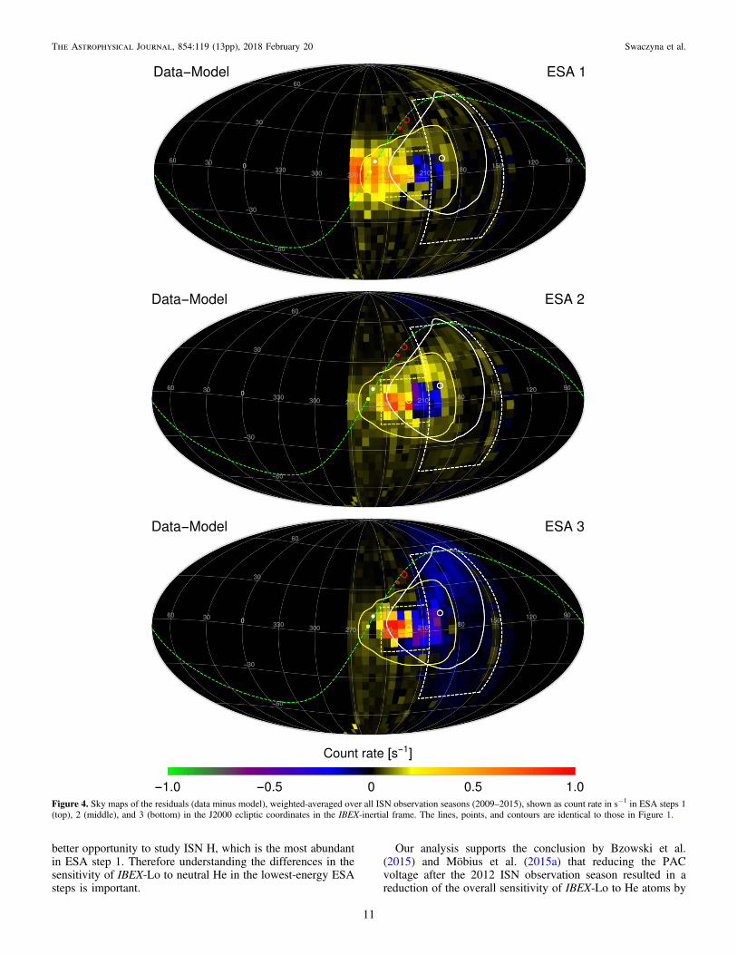
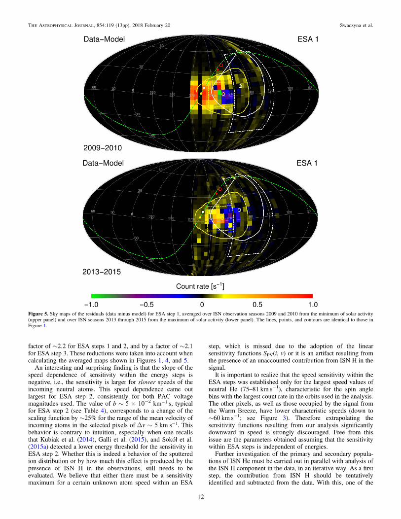
The combination of the model of ISN He obtained now andof the Warm Breeze model from Kubiak et al. (2016) is still notperfect. The most significant issue is likely the presence of ISNH in the data. This hypothesis is based on analysis of residuals,i.e., difference between the count rates in the data and themodel. Maps of these residuals, averaged over all observationseasons, are presented in Figure 4 separately for the three ESAsteps. The yellow, orange, and red colors mark positivedifferences, i.e., an excess of the data over the model. Asclearly seen, this excess is mostly located in the region whereISN H is expected based on modeling of the ISN H signal (see,e.g., Kubiak et al. 2013). This is also in qualitative agreementwith data analyses in Saul et al. (2012, 2013) and Schwadronet al. (2013). Both the magnitude and spatial range of theexcess are reduced when going from ESA steps 1–3 and theyevolve with time, as is clearly implied from a comparison of themap of the residuals for ESA step 1, ISN observation seasons2009 and 2010, shown in the upper panel of Figure 5, withthose obtained for ISN seasons 2013 through 2015, shown inthe lower panel of this figure.

It is important to note that the residual excess is present at alltimes, which suggests that it is indeed due to the physicalreason just discussed and not necessarily to an inadequacy ofthe adopted model of the ISN He and Warm Breeze.Furthermore, the intensity of the excess qualitatively conformswith the expectations for the evolution of ISN H flux during thesolar cycle, with a stronger signal expected during low solaractivity and a reduction in the signal strength when the activityincreases (Kubiak et al. 2013). In our case, the excess for theISN seasons 2009 and 2010 is larger than that for the solarmaximum seasons 2013–2015. This is understandable becauseduring 2009 and 2010 the Sun had just emerged from aprolonged minimum of activity when both solar radiationpressure acting on interstellar H and the ionization losses werelowest. By contrast, during 2013–2015 ISN seasons the Sunwas at the maximum of its activity and both the high ionizationrate (see Figure 31 in McComas et al. 2017) and high radiationpressure reduced the flux of ISN H at 1au considerably. As aresult, the flux of ISN H at 1au during this time is expected tobe lower than during the minimum of solar activity.

The magnitude of the residuals likely underestimates the truemagnitude of the ISN H contribution to the observed signal.This is because the fitting procedure aims to fit the data to themodel as well as possible within the adopted model, which inour case does not include ISN H. The fitting procedure we have

used does not take into account possible systematic patterns inthe residuals. In the case of a perfect fit, with all signalcomponents taken into account, the spatial distribution ofpositive and negative residual values should be random. In ourcase, evidently connected regions of negative and positiveresiduals exist. The region of positive residuals extends wellbeyond the data subset used in the fitting. These are indicationsthat the model, which only includes the primary ISN Hepopulation and the Warm Breeze, is missing an extracomponent, which is likely ISN H. Since, however, theoptimization procedure seeks to have the mean value of theresiduals close to zero, some counts due to ISN H wereinadvertently attributed to ISN He. Therefore it is notrecommended to adopt the residuals as a signal from ISN Hat face value. The true contributions from ISN H must beassessed separately, based on a model that contains allcomponents ISN H, ISN He, and the Warm Breeze. Moreover,the residuals to the right of the ISN He peak show a cluster ofpixels with negative values surrounded by pixels with positivevalues in ESA steps 1 and 2. The same region showspredominantly negative residuals in ESA step 3. It suggeststhat the model of the Warm Breeze also needs to be revised.The presence of neutral H in the signal during all ISN

observation seasons suggests that before further analysis ofdetails of ISN He and the Warm Breeze the question of ISN Hmust be addressed. This topic was discussed by Schwadronet al. (2013) and Katushkina et al. (2015), who pointed out thatthe ratio of counts from ISN H actually observed in ESA steps1 and 2 is significantly different from that expected from stateof the art models of ISN H in the heliosphere and that the likelyculprit is an inadequate knowledge of the solar Lyα radiationpressure, in particular of the spectral profile of this line.Analysis of the largest currently available data set of full-disksolar Lyα line profiles by Kowalska-Leszczynska et al. (2018)(43 profiles measured during various phases of solar activity)showed that, indeed, the central reversal of the profile is deeperthan that used by Katushkina et al. (2015), who adopted amodel by Tarnopolski & Bzowski (2009), which had beendeveloped based on just nine profiles then available. Analysisof the implications of this finding for the ISN H signal expectedfrom IBEX-Lo is underway now.The question of the sensitivity of IBEX-Lo to He atoms in

various ESA steps is interesting mostly in the studies of thesecondary population of ISN He, i.e., the Warm Breeze.Studying the energy spectrum of the Warm Breeze maypotentially bring a better insight into the plasma flow andtemperature in the outer heliosheath. Also, as shown by ourresults, expanding the analysis of ISN He from one to threeESA steps improves the statistics. Additionally, one obtains a

Table 5ISN He Flow Parameters from Different Studies of IBEX Data

Reference λ(°) β(°) v (km s−1) T (K)

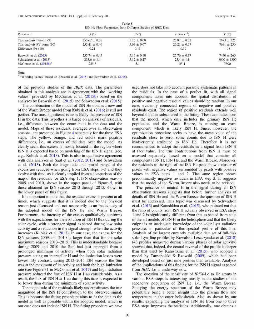
This analysis P-norm (9) 255.62±0.36 5.16±0.08 25.82±0.33 7673±225This analysis PV-norm (10) 255.41±0.40 5.03±0.07 26.21±0.37 7691±230Difference (9)–(10) 0.21 0.13 −0.39 −18

Bzowski et al. (2015) 255.74±0.45 5.16±0.10 25.76±0.37 7440±260Schwadron et al. (2015) 255.6±1.4 5.12±0.27 25.4±1.1 8000±1300McComas et al. (2015b)a 255.7 5.1 25.4 7500

Note.a“Working values” based on Bzowski et al. (2015) and Schwadron et al. (2015).

10

The Astrophysical Journal, 854:119 (13pp), 2018 February 20 Swaczyna et al.

better opportunity to study ISN H, which is the most abundantin ESA step 1. Therefore understanding the differences in thesensitivity of IBEX-Lo to neutral He in the lowest-energy ESAsteps is important.

Our analysis supports the conclusion by Bzowski et al.(2015) and Möbius et al. (2015a) that reducing the PACvoltage after the 2012 ISN observation season resulted in areduction of the overall sensitivity of IBEX-Lo to He atoms by

Figure 4. Sky maps of the residuals (data minus model), weighted-averaged over all ISN observation seasons (2009–2015), shown as count rate in s−1 in ESA steps 1(top), 2 (middle), and 3 (bottom) in the J2000 ecliptic coordinates in the IBEX-inertial frame. The lines, points, and contours are identical to those in Figure 1.

11

The Astrophysical Journal, 854:119 (13pp), 2018 February 20 Swaczyna et al.

factor of ∼2.2 for ESA steps 1 and 2, and by a factor of ∼2.1for ESA step 3. These reductions were taken into account whencalculating the averaged maps shown in Figures 1, 4, and 5.

An interesting and surprising finding is that the slope of thespeed dependence of sensitivity within the energy steps isnegative, i.e., the sensitivity is larger for slower speeds of theincoming neutral atoms. This speed dependence came outlargest for ESA step 2, consistently for both PAC voltagemagnitudes used. The value of b∼5×10−2 km s1- , typicalfor ESA step 2 (see Table 4), corresponds to a change of thescaling function by ∼25% for the range of the mean velocity ofincoming atoms in the selected pixels of v 5 km s 1D ~ - . Thisbehavior is contrary to intuition, especially when one recallsthat Kubiak et al. (2014), Galli et al. (2015), and Sokół et al.(2015a) detected a lower energy threshold for the sensitivity inESA step 2. Whether this is indeed a behavior of the sputteredion distribution or by how much this effect is produced by thepresence of ISN H in the observations, still needs to beevaluated. We believe that either there must be a sensitivitymaximum for a certain unknown atom speed within an ESA

step, which is missed due to the adoption of the linearsensitivity functions SPV(i, v) or it is an artifact resulting fromthe presence of an unaccounted contribution from ISN H in thesignal.It is important to realize that the speed sensitivity within the

ESA steps was established only for the largest speed values ofneutral He (75–81 km s−1), characteristic for the spin anglebins with the largest count rate in the orbits used in the analysis.The other pixels, as well as those occupied by the signal fromthe Warm Breeze, have lower characteristic speeds (down to∼60 km s−1; see Figure 3). Therefore extrapolating thesensitivity functions resulting from our analysis significantlydownward in speed is strongly discouraged. Free from thisissue are the parameters obtained assuming that the sensitivitywithin ESA steps is independent of energies.Further investigation of the primary and secondary popula-

tions of ISN He must be carried out in parallel with analysis ofthe ISN H component in the data, in an iterative way. As a firststep, the contribution from ISN H should be tentativelyidentified and subtracted from the data. With this, one of the

Figure 5. Sky maps of the residuals (data minus model) for ESA step 1, averaged over ISN observation seasons 2009 and 2010 from the minimum of solar activity(upper panel) and over ISN seasons 2013 through 2015 from the maximum of solar activity (lower panel). The lines, points, and contours are identical to those inFigure 1.

12

The Astrophysical Journal, 854:119 (13pp), 2018 February 20 Swaczyna et al.

parameter sets from the fits we have obtained in this papershould be adopted and the model signal due to ISN He shouldbe computed and subtracted from the data. Subsequently, a newparameter set for the Warm Breeze fitted should be fitted to theresulting data set, and the resulting Warm Breeze model used inthe next iteration of parameter fitting for ISN He and ISN H.

5. Summary

We have analyzed observations of ISN He carried out byIBEX during the ISN He observation seasons 2009 through2015, for the first time using information from IBEX-Lo ESAsteps 1 through 3. We have established the differences in thesensitivity to ISN He atoms in these ESA steps and thesensitivity change due to the change in the IBEX-Lo PACvoltage setting that was introduced after the 2012 ISN season.We found that the overall sensitivity increases from lowerenergy steps to the higher ones. Surprisingly, however, wefound that the sensitivity within all these ESA steps may be adecreasing function of atom speed. We are currently unable toverify if this is a true effect or a result of the presence of countsdue to ISN H in the signal.

The excesses of the measured count rates over the modeledsignal on the left side of the ISN He peak position in all ESAsteps suggests that the data may be partially contaminated byISN H atoms. We suggest that the signal due to ISN H must bequantitatively interpreted and subtracted before information onthe Warm Breeze, available in the measurements in ESA steps1–3, can be fully utilized. Finally, we found that the bulkvelocity vector and temperature of ISN He obtained in thepresent analysis using data from ESA steps 1–3, listed in thelast two rows in Table 2, are within the fit uncertainties of theseparameters obtained by Bzowski et al. (2015) from the analysisusing only data from ESA step 2. Further analysis of theprimary and secondary populations of ISN He and ISN Hshould be carried out iteratively, using parameters of thesepopulations obtained in a preceding step of the analysis in thesubsequent steps.

This study was supported by the grant 2015/18/M/ST9/00036 from the National Science Center, Poland. P.S. is supportedby the Foundation for Polish Science (FNP). Work in the USAand the IBEX data were supported by the IBEX mission as a partof NASA’s Explorer Program, grant NNG05EC85C.

ORCID iDs

Paweł Swaczyna https://orcid.org/0000-0002-9033-0809Maciej Bzowski https://orcid.org/0000-0003-3957-2359André Galli https://orcid.org/0000-0003-2425-3793David J. McComas https://orcid.org/0000-0002-9745-3502Eberhard Möbius https://orcid.org/0000-0002-2745-6978

Nathan A. Schwadron https://orcid.org/0000-0002-3737-9283P. Wurz https://orcid.org/0000-0002-2603-1169

References

Baranov, V. B., & Malama, Y. G. 1995, JGR, 100, 1461Bzowski, M., Kubiak, M. A., Czechowski, A., & Grygorczuk, J. 2017, ApJ,

845, 15Bzowski, M., Kubiak, M. A., Hłond, M., et al. 2014, A&A, 569, A8Bzowski, M., Kubiak, M. A., Möbius, E., et al. 2012, ApJS, 198, 12Bzowski, M., Sokół, J. M., Tokumaru, M., et al. 2013, in Cross-Calibration of

Far UV Spectra of Solar Objects and the Heliosphere, ISSI Scientific ReportNo. 13, ed. E. Quémerais, M. Snow, & R. Bonnet (New York: Springer), 67

Bzowski, M., Swaczyna, P., Kubiak, M., et al. 2015, ApJS, 220, 28Frisch, P. C., Redfield, S., & Slavin, J. D. 2011, ARA&A, 49, 237Funsten, H. O., DeMajistre, R., Frisch, P. C., et al. 2013, ApJ, 776, 30Fuselier, S. A., Allegrini, F., Bzowski, M., et al. 2012, ApJ, 754, 14Fuselier, S. A., Bochsler, P., Chornay, D., et al. 2009, SSRv, 146, 117Galli, A., Wurz, P., Park, J., et al. 2015, ApJS, 220, 30Galli, A., Wurz, P., Schwadron, N., et al. 2016, ApJ, 821, 107Galli, A., Wurz, P., Schwadron, N., et al. 2017, ApJ, 851, 2Katushkina, O. A., Izmodenov, V. V., & Alexashov, D. B. 2015, MNRAS,

446, 2929Katushkina, O. A., Izmodenov, V. V., Alexashov, D. B., Schwadron, N. A., &

McComas, D. J. 2015, ApJS, 220, 33Kowalska-Leszczynska, I., Bzowski, M., Sokół, J. M., & Kubiak, M. A. 2018,

ApJ, 852, 115Kubiak, M. A., Bzowski, M., Sokół, J. M., et al. 2013, A&A, 556, A39Kubiak, M. A., Bzowski, M., Sokół, J. M., et al. 2014, ApJS, 213, 29Kubiak, M. A., Swaczyna, P., Bzowski, M., et al. 2016, ApJS, 223, 25Leonard, T. W., Möbius, E., Bzowski, M., et al. 2015, ApJ, 804, 42McComas, D., Bzowski, M., Frisch, P., et al. 2015a, ApJ, 801, 28McComas, D., Bzowski, M., Fuselier, S., et al. 2015b, ApJS, 220, 22McComas, D. J., Allegrini, F., Bochsler, P., et al. 2009, SSRv, 146, 11McComas, D. J., Carrico, J. P., Hautamaki, B., et al. 2011, SpWea, 9, 11002McComas, D. J., Zirnstein, E. J., Bzowski, M., et al. 2017, ApJS, 229, 41Möbius, E., Bochsler, P., Heirtzler, D., et al. 2012, ApJS, 198, 11Möbius, E., Bzowski, M., Fuselier, S. A., et al. 2015a, ApJS, 220, 24Möbius, E., Bzowski, M., Fuselier, S. A., et al. 2015b, J. Phys. Conf. Ser., 577,

012019Möbius, E., Kucharek, H., Clark, G., et al. 2009, SSRv, 146, 149Park, J., Kucharek, H., Möbius, E., et al. 2015, ApJS, 220, 34Park, J., Kucharek, H., Möbius, E., et al. 2016, ApJ, 833, 130Ruciński, D., Bzowski, M., & Fahr, H. J. 2003, AnGeo, 21, 1315Saul, L., Bzowski, M., Fuselier, S., et al. 2013, ApJ, 767, 130Saul, L., Wurz, P., Möbius, E., et al. 2012, ApJS, 198, 14Schwadron, N., Möbius, E., Leonard, T., et al. 2015, ApJS, 220, 25Schwadron, N. A., Moebius, E., Fuselier, S., et al. 2014, ApJS, 215, 13Schwadron, N. A., Moebius, E., Kucharek, H., et al. 2013, ApJ, 775, 86Sokół, J. M., & Bzowski, M. 2014, arXiv:1411.4826Sokół, J. M., Bzowski, M., Kubiak, M., et al. 2015a, ApJS, 220, 29Sokół, J. M., Bzowski, M., Kubiak, M., & Möbius, E. 2016, MNRAS,

458, 3691Sokół, J. M., Kubiak, M., Bzowski, M., & Swaczyna, P. 2015b, ApJS, 220, 27Swaczyna, P., Bzowski, M., Kubiak, M., et al. 2015, ApJS, 220, 26Tarnopolski, S., & Bzowski, M. 2009, A&A, 493, 207Wieser, M., & Wurz, P. 2005, MeScT, 16, 2511Witte, M. 2004, A&A, 426, 835Wood, B. E., Müller, H.-R., & Witte, M. 2015, ApJ, 801, 62Wurz, P., Saul, L., Scheer, J. A., et al. 2008, JAP, 103, 054904Wurz, P., Scheer, J., & Wieser, M. 2006, J. Surf. Sci. Nanotechnol., 4, 394Zirnstein, E. J., Heerikhuisen, J., Funsten, H. O., et al. 2016, ApJL, 818, L18

13

The Astrophysical Journal, 854:119 (13pp), 2018 February 20 Swaczyna et al.