Embed Size (px)
Citation preview
INTERPRETIVE THREE-DIMENSIONAL NUMERICAL GROUNDWATER FLOW
MODELING, ROARING SPRINGS, GRAND CANYON, ARIZONA
by Lanya E. V. Ross
A Thesis
Submitted in Partial Fulfillment
of the Requirements for the Degree of
Master of Science
in Geology
Northern Arizona University
December 2005
Approved:
_____________________________________ Abraham E. Springer, Ph.D., Chair _____________________________________ Ronald C. Blakey, Ph.D.
_____________________________________ Roderic A. Parnell Jr., Ph.D.
ii
ABSTRACT
INTERPRETIVE THREE-DIMENSIONAL NUMERICAL GROUNDWATER FLOW MODELING, ROARING SPRINGS, GRAND CANYON, ARIZONA
LANYA E. ROSS
The Redwall-Muav aquifer (R-aquifer), an unconfined karstified carbonate
aquifer, discharges through large springs in Grand Canyon. The largest R-aquifer springs
in Grand Canyon are on the North Rim and include Roaring Springs, the sole municipal
water supply for Grand Canyon National Park. This study provided new data and
synthesized existing information about the R-aquifer where it discharges from Roaring
Springs, providing information for source water protection and acting as a model for the
larger R-aquifer system on the Kaibab Plateau. In 2003, temporary stream gaging stations
were established with pressure transducers in the stream channel below Roaring Springs
and in Roaring Springs cave. Discharge was measured on a monthly basis through the
summer monsoon, and two stage-discharge curves were constructed to calculate
discharge in the stream (stage-discharge R2 = 0.53) and in the cave (stage-discharge R2 =
0.35) between March and December 2003. The quality of the stage-discharge
relationships was primarily affected by the roughness of the stream channel and the
effects of barometric pressure changes in Roaring Springs cave.
In addition, monthly water samples were collected from the spring for δ18O/δ2H
and tritium analyses to constrain recharge rates and groundwater flow paths. These data,
combined with improvements in Grand Canyon geologic maps, were used to construct a
digital geologic framework model (DGFM), a conceptual model and a numerical
iii
groundwater flow model of the Roaring Springs system. The final datasets were
displayed with a GeoWall (a digital three-dimensional projection system) to test its
applicability for hydrologic education.
Results indicate that groundwater flow to Roaring Springs is very localized,
particularly when compared to springs recharge areas on the South Rim of Grand
Canyon. The Roaring Springs recharge area is estimated to be no larger than 30 km2.
Roaring Springs requires most of the winter snow pack to sustain perennial flow (~70%
annual precipitation), as little to no recharge occurs during the summer monsoon.
Recharging groundwater moves through the aquifer along two principal pathways which
are apparent on the Roaring Springs hydrograph base flow recession curves. Water
flowing through the conduit system moves from the surface to Roaring Springs in less
than a month, possibly within a day. Water moving through the larger aquifer matrix
moves more slowly, with travel times ranging from months to years. Mean groundwater
residence time is ~7 years, based on tritium analysis of spring water.
Attempts to display the Roaring Springs groundwater system on the Kaibab
Plateau with GeoWall technology met with limited success. The difference in scale
between spring recharge area and the Kaibab Plateau as a whole made them difficult to
view in tandem.
iv
ACKNOWLEDGEMENTS
The study was partially funded through a Geological Society of America research
grant, a grant from the Colorado Plateau Stable Isotope Laboratory, the NAU Geology
Department L.B.C. McCulloch award, a Northern Arizona University Geology
Department Undergraduate mentorship scholarship, and support from Steve Finch of
John Shomaker and Associates, Inc. Research was completed under National Park
Service Scientific and Collecting Permit GRCA-2002-SCI-0019. John Rihs of Grand
Canyon National Park provided data and equipment to the study. Bruce Aiken of Grand
Canyon National Park was an invaluable resource for data, project support, and access to
the study site.
I wish to thank the many people who contributed to the completion of this thesis.
Foremost among them is Dr. Abe Springer. I would also like to thank Drs. Ronald C.
Blakey and Roderic A. Parnell, Jr. for editing the study report and serving on my
committee. Thanks to Donald Bills at the USGS in Flagstaff, who provided unpublished
Grand Canyon spring discharge data for this study. Many Northern Arizona University
students assisted in fieldwork, and deserve special thanks: Jeremy Kobor and Siobhan
McConnell, Amy Welte-Bernard, Meg (Palevich) Varhalmi, and the notorious Jacob
Miller.
Finally, I would like to thank Ben Hinkley, whose wide-ranging and unending
support was so important that I married him.
v
TABLE OF CONTENTS
ABSTRACT........................................................................................................................ ii
ACKNOWLEDGEMENTS............................................................................................... iv
LIST OF TABLES............................................................................................................ vii
LIST OF FIGURES ......................................................................................................... viii
LIST OF APPENDICES..................................................................................................... x
CHAPTER 1: INTRODUCTION....................................................................................... 1
Purpose and Objectives................................................................................................... 2 Significance of Problem.................................................................................................. 3 Study Area Location ....................................................................................................... 4 Previous Investigations ................................................................................................... 6
CHAPTER 2: DIGITAL GEOLOGIC FRAMEWORK MODEL ................................... 11
Purpose and Objectives................................................................................................. 11 Model Construction Methodology................................................................................ 11
Software .................................................................................................................... 11 Data Sources ............................................................................................................. 12 Process ...................................................................................................................... 13
Discussion and Conclusions ......................................................................................... 20 CHAPTER 3: CONCEPTUAL GROUNDWATER FLOW MODEL............................. 24
Purpose and Objectives................................................................................................. 24 Data Collection Methodology....................................................................................... 24 Conceptual Model Boundaries...................................................................................... 29 Hydrostratigraphic Units............................................................................................... 29
Stratigraphy............................................................................................................... 31 Structural Geology.................................................................................................... 41
vi
Water Budget ................................................................................................................ 47 Precipitation .............................................................................................................. 47 Evapotranspiration .................................................................................................... 49 Spring Discharge....................................................................................................... 52 Runoff ....................................................................................................................... 64 Recharge ................................................................................................................... 70 Change in Aquifer Storage........................................................................................ 77
Flow System ................................................................................................................. 77 Groundwater Flow Direction .................................................................................... 78 Groundwater Flow Rates .......................................................................................... 84
Conclusions and Discussion ......................................................................................... 89 CHAPTER 4: NUMERICAL GROUNDWATER FLOW MODEL ............................... 93
Purpose and Objectives................................................................................................. 93 Model Code................................................................................................................... 94 Model Construction ...................................................................................................... 94
Time and Space......................................................................................................... 95 Model Grid................................................................................................................ 95 Model Boundaries..................................................................................................... 95 Model Parameters ..................................................................................................... 97
Model Calibration ....................................................................................................... 101 Calibration Targets.................................................................................................. 101 Calibration Process ................................................................................................. 101
Sensitivity Analysis .................................................................................................... 106 Model Limitations....................................................................................................... 108 Conclusions and Discussion ....................................................................................... 109
CHAPTER 5: SUMMARY AND DISCUSSION .......................................................... 110
BIBLIOGRAPHY........................................................................................................... 113
APPENDICES ................................................................................................................ 120
vii
LIST OF TABLES Table 1. Mean monthly precipitation (1925-1998), Bright Angel Ranger Station, AZ ... 49
Table 2. Mean monthly maximum and minimum temperatures (°C), Bright Angel Ranger Station, AZ................................................................................................................ 49
Table 3. Typical vegetation zones of the Grand Canyon by elevation range ................... 49
Table 4. Historic discharge measurements at Roaring Springs, Kaibab Plateau, AZ....... 54
Table 5. 2003 discharge measurements at Roaring Springs, Kaibab Plateau, AZ............ 55
Table 6. Tritium concentrations (TU) at Roaring Springs cave........................................ 88
Table 7. Qualitative interpretation of tritium data. ........................................................... 88
Table 8. 2003 Roaring Springs conceptual water budget. ................................................ 90
Table 9. Annual water budget for Roaring Springs groundwater flow model. .............. 103
Table 10. Parameters and stresses in calibrated Roaring Springs flow model. .............. 103
viii
LIST OF FIGURES
Figure 1. Location of the study area on the Kaibab Plateau, Arizona.. ............................. 5
Figure 2. Basal geologic contact elevation data point distribution for the Kaibab and Muav formations....................................................................................................... 16
Figure 3. Semivariogram models used in the kriging interpolation method..................... 17
Figure 4. Variance grid generated by ArcView 3.2 GIS .................................................. 18
Figure 5. Geologic cross-sections constructed across the Kaibab Plateau using the digital geologic framework model ....................................................................................... 19
Figure 6. Paleozoic geologic surfaces of the southern Kaibab Plateau, AZ..................... 21
Figure 7. Location of sites sampled in Roaring Springs Canyon in 2003. ....................... 26
Figure 8. Stream channel cross section of Roaring Springs stream.................................. 27
Figure 9. Conceptual model boundaries of the Roaring Springs flow system.................. 30
Figure 10. Roaring Springs Canyon hydrostratigraphy, Kaibab Plateau, AZ. ................. 32
Figure 11. Major faults and folds on the Kaibab Plateau, AZ .......................................... 43
Figure 12. Geologic cross-section of the East Kaibab Monocline in Grand Canyon ....... 46
Figure 13. Kaibab Plateau spring locations ..................................................................... 53
Figure 14. Discharge-discharge relationship between Roaring Springs and Bright Angel Creek, Grand Canyon, AZ. ....................................................................................... 57
Figure 15. Roaring Springs stage-discharge relationship ................................................ 58
Figure 16. Roaring Springs discharge-turbidity relationship............................................ 59
Figure 17. Stage-discharge relationship between Roaring Springs Stream and Roaring Springs Cave, Kaibab Plateau, AZ............................................................................ 61
Figure 18. 2003 spring discharge, Roaring Springs, Kaibab Plateau, AZ. ....................... 62
Figure 19. Daily discharge comparison between Roaring Springs and Bright Angel Creek, Grand Canyon, AZ. ....................................................................................... 63
Figure 20. Roaring Springs stream surface watershed, Kaibab Plateau, AZ.................... 65
ix
Figure 21. Comparison of 2003 daily precipitation and discharge, Roaring Springs Stream, Kaibab Plateau, AZ...................................................................................... 67
Figure 22. Roaring Springs discharge between March 7 and March 28, 2003 showing effects of snowmelt on stream discharge .................................................................. 68
Figure 23. Roaring Springs stream and cave hydrographs ............................................... 69
Figure 24. Photograph of Kaibab Plateau sinkhole .......................................................... 71
Figure 25. Sinkhole watersheds on the Kaibab Plateau, AZ............................................. 72
Figure 26. 2003 Roaring Springs hydrograph illustrating the effect of seasonal recharge on the Kaibab Plateau, AZ ........................................................................................ 74
Figure 27. Stable isotope analyses of 1993 and 2003-2004 Roaring Springs discharge and Kaibab Plateau precipitation ..................................................................................... 76
Figure 28. Trends in sinkhole distribution versus trends in Bouguer gravity and isostatic gravity data................................................................................................................ 79
Figure 29. 25 km2 watersheds on the basal surface of the Muav Formation. ................... 80
Figure 30. Photograph of R-aquifer in Roaring Springs Canyon, AZ.............................. 82
Figure 31. Modern R-aquifer cave passage orientation for selected caves in Grand Canyon. ..................................................................................................................... 83
Figure 32. Daily spring discharge versus seasonal variation in tritium, δ18O and δ2H in 2003 for Roaring Springs, Kaibab Plateau, AZ. ....................................................... 86
Figure 33. 2003 Roaring Springs seasonal variation in temperature, pH, and specific conductivity............................................................................................................... 87
Figure 35. Initial no-flow boundary conditions for ground water flow model of Roaring Springs. ..................................................................................................................... 98
Figure 36. Maps showing the distribution of hydraulic conductivity and recharge values in the groundwater flow model of Roaring Springs................................................ 100
Figure 37. Final locations of no-flow boundary conditions in groundwater flow model of Roaring Springs. ..................................................................................................... 104
Figure 39. Model sensitivity to recharge and Roaring Springs drain conductance ........ 107

x
LIST OF APPENDICES
Appendix A. Digital Geologic Framework Model grid files (Enclosed CD).
Appendix B. Roaring Springs 2003 field sheets.
Appendix C. Roaring Springs 2003 hydrologic data.
Appendix D. Roaring Springs MODFLOW files (Enclosed CD).

xi
This work is dedicated to my father and grandfather’s strong hearts.
1
CHAPTER 1
INTRODUCTION
The most obvious water feature associated with Grand Canyon is the Colorado
River. Less visible, but equally important from a water resources management
perspective, is the groundwater flow system supplying base flow to the Colorado River
and rare desert spring ecosystems, drinking water to Arizona tourists and residents, and
cultural meaning to tribal communities in and around Grand Canyon.
The primary aquifer in Grand Canyon is the R-aquifer, composed of the Redwall,
Temple Butte and Muav formations. This aquifer extends across much of northern
Arizona, but groundwater movement is bisected by the Colorado River in Grand Canyon.
The result is two separate groundwater systems with similar geologic characteristics but
incredibly different behavior – one on the South Rim and the other on the North Rim.
The South Rim of the Grand Canyon has been the focus of recent groundwater
research, as development pressure (due in particular to tourism in Tusayan, AZ)
continues to grow. Research has included the identification of the seeps and springs along
the South Rim of the Canyon, and the delineation of the major spring recharge areas in
fracture zones on the Coconino Plateau (Montgomery and Associates 1996; Wilson 2000;
Kessler 2002; Stevens 2002b, Kobor 2004; Monroe et al 2004). Spring discharge from
this aquifer is low, but remains stable throughout the year.
Major springs on the North Rim of the Grand Canyon also discharge out of the R-
aquifer, more numerous and larger than those on the South Rim. The discharge rates for
these North Rim springs are commonly believed to fluctuate significantly throughout the
year (Stevens 2002), a conclusion based primarily on observations at Vasey’s Paradise,
2
the only North Rim spring being actively monitored due to its designation as a protected
ecosystem for the endangered Oxyloma haydeni kanabensis (Kanab ambersnail), and its
convenient access at river level from Colorado River boat trips. This fluctuation has not
been adequately documented at other North Rim springs, and this fluctuation has never
been incorporated into groundwater models for the area. This lack of information is of
particular concern when considering that Roaring Springs is the sole source of potable
water for Grand Canyon National Park facilities on the North and South Rims. Under
federal regulation, this spring is regularly monitored as a drinking water supply. Since the
early 1970’s, the amount of water diverted and the turbidity and pH of the water of
Roaring Springs has been monitored daily from May to October. The spring is sampled
every three years for major ion chemistry and other parameters required for drinking
water supplies (Huntoon 2002; Aiken 2003). Interestingly, the total discharge of Roaring
Springs has never been regularly monitored, and limited attempts to date the age of
spring water have been inconclusive. Consequently, the recharge area for Roaring
Springs has never been determined (Rihs 2002).
Purpose and Objectives
The purpose of this study was to gather new data and to synthesize existing
information about the R-aquifer where it discharges from Roaring Springs in Grand
Canyon, Arizona. A new conceptual model was created using recently developed three-
dimensional visualization software to develop a more cohesive picture of the aquifer
structure and to make it more available in an easily understandable format for the sake of
park hydrologists, managers, and visitors.
3
The purpose was accomplished through completion of the following objectives:
1) Develop a digital geologic framework model for the Kaibab Plateau,
2) Construct and calibrate a numerical groundwater flow model for the Redwall
Muav aquifer on the Kaibab Plateau, and
3) Incorporate both the geologic framework model and the groundwater flow model
into three-dimensional computer visualization software for community outreach
and technology transfers.
Significance of Problem
Recent South Rim models indicate that most groundwater movement through the
R-aquifer on the Coconino Plateau is through faults and fractures. The system directs
water toward three major discharge points on the South Rim: Havasu Spring, Hermit
Spring, and Indian Garden Spring (Montgomery and Associates 1996; Wilson 2000;
Kessler 2002). No such equivalent work has been done on the North Rim, even though
Roaring Springs, on the North Rim, is Grand Canyon National Park’s municipal water
supply, providing water to over 4 million annual visitors and year-round employees
(http://www.nps.gov/grca/). The karst springs on the North Rim also provide significant
perennial base flow to the Colorado River, as well as supporting havens of biodiversity in
the arid to semi-arid Grand Canyon along tributary canyons. Only 0.003% of the area in
Grand Canyon National Park is occupied by tributary streams, but these streams support
36% of the Canyon’s total riparian flora (Hart et al 2002b).
Lack of planned development on the North Rim of the Grand Canyon ensures a
low probability of impacting spring discharge quantity in the future. However, rapid
4
groundwater recharge through fault and fracture systems may mean that land use
occurring north of the park boundaries could significantly impact water quality.
A comparison of springs on the North and South Rims of the Grand Canyon may
also provide insight into the rate and process of karst development on the Colorado
Plateau. Due to the higher elevation of the North Rim, annual precipitation is
approximately 250 mm (10 inches) greater there than on the South Rim. This project
may help to quantify the level of karst development, which has been determined to be a
critical part of future work at the Grand Canyon (Rihs 2000; Huntoon 1974).
Study Area Location
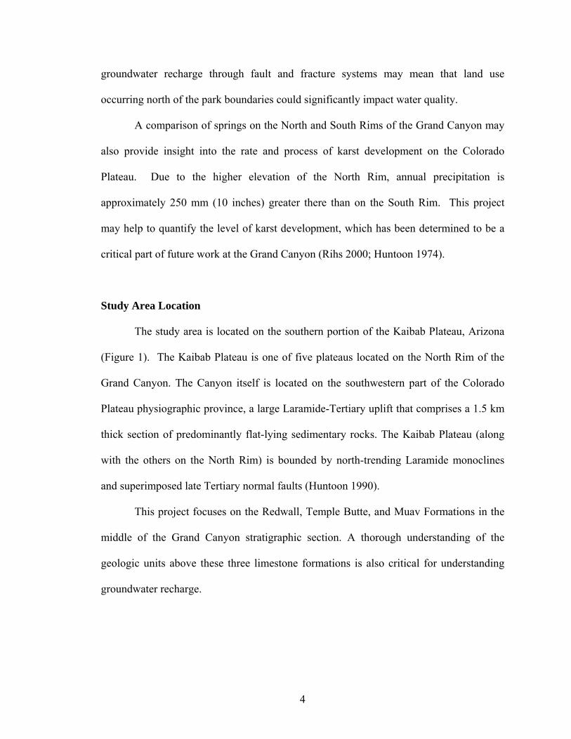
The study area is located on the southern portion of the Kaibab Plateau, Arizona
(Figure 1). The Kaibab Plateau is one of five plateaus located on the North Rim of the
Grand Canyon. The Canyon itself is located on the southwestern part of the Colorado
Plateau physiographic province, a large Laramide-Tertiary uplift that comprises a 1.5 km
thick section of predominantly flat-lying sedimentary rocks. The Kaibab Plateau (along
with the others on the North Rim) is bounded by north-trending Laramide monoclines
and superimposed late Tertiary normal faults (Huntoon 1990).
This project focuses on the Redwall, Temple Butte, and Muav Formations in the
middle of the Grand Canyon stratigraphic section. A thorough understanding of the
geologic units above these three limestone formations is also critical for understanding
groundwater recharge.
5
Figure 1. Location of the study area on the Kaibab Plateau, Arizona. Springs discharging
from the R-aquifer on the North Rim of Grand Canyon are sized according to relative
discharge. Base map modified from Billingsley and Hampton (2000).
6
Previous Investigations
Working in Grand Canyon is a challenging task but one that has appealed to many
scientists since the mid-1800’s. The result is that much hydrogeologic data exist for the
Grand Canyon; but these data are sporadic, often incompatible with other data sets, and
difficult to find. This section provides an overview of previous Grand Canyon research
which applies to the groundwater flow system through the R-aquifer. This is by no means
a complete list of Grand Canyon geologic resources, which are too numerous to mention
here. Rather, these sources have provided specific information during this study.
The Grand Canyon Wildlands Council, Inc. (Stevens 2001) summarized the
extent and quality of existing data regarding seeps, springs, and ponds on the Arizona
Strip. This report is concerned with the distribution and quality of spring ecosystems; it
briefly presents hydrogeologic research along the Arizona Strip, summarizes land use,
presents biological resource data, and presents case studies that include Vaseys Paradise.
There is a notable absence of data regarding conceptual groundwater models for springs
discharging below the Supai Group on the north side of Grand Canyon.
The United States Geological Survey (USGS) (Johnson and Sanderson 1968)
published a compilation of all known spring and tributary stream discharge and chemistry
data. This report briefly describes all springs visited during a ten-day boat trip from Lees
Ferry to Pierce Ferry in 1960 and compiles all known additional discharge data for
springs in Grand Canyon collected since 1923. In order to maximize the value of the
sparse data set, discharge relationships were developed between Bright Angel Creek and
Roaring Springs, between Thunder River flow and Tapeats Creek discharge, and between
Bright Angel and Tapeats Creeks.
7
The USGS report undoubtedly shaped subsequent spring research by Huntoon
(1970). His primary interest was karst development in the R-aquifer, although he also
produced geologic cross-sections, measured spring and stream discharge, and created a
two-dimensional, steady-state finite difference model of the southern Kaibab Plateau. He
provided a few more discharge data points for North Rim springs, but his work is most
notable for improving the conceptual model of groundwater flow through a better
understanding of the Kaibab Plateau’s structural geology. His investigation of fractures
sets in the R-aquifer led him to conclude that the karst springs connected to these
structural features drain approximately 60% of the plateau. He continued to study the
structural development of eastern Grand Canyon as well as karst development in the
Redwall Limestone, paying particular attention to the stages of karst development evident
in Redwall cave systems of varying ages (Huntoon 1970; 1974; 2000).
In the early 1970’s the Grand Canyon’s current public water supply system was
completed, with a pump house at Roaring Springs supplying water to North Rim park
facilities and a trans-canyon pipeline funneling spring water to Phantom Ranch and the
pump house at Indian Gardens. From approximately April to October of each year, park
service staff record the daily volume of water diverted and pumped from the spring, the
turbidity, and pH. The spring is sampled every three years for major ion chemistry and
other parameters required for drinking water supplies (Aiken 2003). Very little of these
data were available for this project. Most of the paper files are located at the Roaring
Springs pump house and there was limited time to assist with data entry on field trips to
collect spring discharge and water samples.
8
Foust and Hoppe (1985) analyzed a ten-year span of spring and tributary stream
chemistry in Grand Canyon with the purpose of identifying long-term seasonal trends and
baseline chemical concentrations. Many samples were taken at sites both near the springs
and near the Colorado River to understand how water chemistry changed due to exposure
to different geologic formations. North Rim sources in this study included: Bright Angel
Creek, Clear Creek, Deer Creek, Manzanita Creek, Phantom Creek, Ribbon Creek,
Roaring Springs, Tapeats Creek, Thunder River, Transept Creek, and Wall Creek. Seven
water samples were collected at Roaring Springs between 1975 and 1981; most were
collected between June of 1980 and February of 1981.
Further chemical analysis of Grand Canyon spring water was published by
Zukosky (1995). Her work focused on springs, groundwater, and surface water on the
South Rim of the Grand Canyon. She analyzed field measurements, major anions,
selected trace-element concentrations, and ratios of the stable isotopes of oxygen and
hydrogen. Her results quantified chemical similarities between springs discharging from
similar lithologic units and/or geographic localities. She also concluded that local
groundwater has similar chemistry to the springs, particularly those issuing from the
Redwall-Muav limestone. Roaring Springs was the only North Rim source that she
analyzed for stable isotopes of oxygen and hydrogen, and she found that this water source
is significantly more isotopically depleted than South Rim water sources, implying a
different origin.
Crossey (2002) published a report that examined spring chemistry above and
below the Great Unconformity in Grand Canyon to better understand groundwater
circulation and travertine formation throughout the entire stratigraphic section.
9
Grand Canyon National Park is currently working with the USGS on a newly
created spring sampling protocol on the South Rim (Rihs 2000; Hart et al 2002b). Springs
are sampled for stable isotopes of carbon, oxygen, hydrogen, and strontium. Samples are
also analyzed for tritium. Initial results substantiate South Rim groundwater flow
modeling work indicating long flow paths. Sporadic discharge data are available for
North Rim springs. The USGS published a compilation of spring data in 1968, and they
are currently updating this (Rihs 2002).
Detailed descriptions of the geologic units in Grand Canyon are available in many
volumes and maps (McKee and Gutschick 1969; Huntoon 1970; Beus and Morales 1990;
Billingsley and Hampton 2000; Billingsley and Hampton 2001; Billingsley and
Wellmeyer 2001a, b; Wellmeyer 2001). Tindall’s (2000a, b) studies of the structural
deformation of the East Kaibab Monocline provided valuable insight regarding the
orientation and character of faulting and fracturing on the Kaibab Plateau, relating to
groundwater flow pathways. Cepeda (1994) used Landsat images and fieldwork to map
fracture orientations and distribution on the Kaibab Plateau. This map was then used to
contour fracture density and fracture intersection density, which may have implications
for the source area and volume of groundwater recharge. Gettings and Bultman (2005)
explored the potential to use geophysical data and GIS technology to predict the
occurrence of deep penetrative fractures in Grand Canyon National Park; their results can
be used to predict groundwater flow pathways.
In 1996, Montgomery and Associates (Victor and Montgomery 2000) created a
three-dimensional, transient groundwater model as part of the Tusayan, Arizona
environmental impact assessment. In a parallel study, Wilson (2000) built a steady-state
10
three-dimensional groundwater model for the Coconino Plateau using Stratamodel. This
included the delineation for spring-sheds on the South Rim of the Canyon. Similarly,
Kessler (2002) modeled the Coconino Plateau using a finer resolution model coupled
with ArcView software (ArcGIS 3D Analyst) and MODFLOW to create a model that
was easily accessible to the public. These publications all tested the ability of
MODFLOW to realistically predict groundwater flow regimes in the R-aquifer on the
Colorado Plateau and yielded information regarding the relationship between structure,
stratigraphy, and hydrogeology.
As groundwater flow models are being used more often as planning tools, a
debate is ongoing regarding their validity. This is of particular concern in karst aquifers,
where porous media models such as MODFLOW may not be appropriate. Scanlon et al
(2003) concluded that porous media models can generate reasonable results if the study
area is large enough to justify averaging values of permeability. Regional scale
groundwater flow models of karst aquifers are commonly used for water budget analyses
(Diodato 1994; Knochenmus and Robinson 1996; Quinn and Tomasko 2002; Smith and
Hunt 2004). These models may not adequately simulate contaminant flow pathways,
however (Diodato 1994; Ginsberg and Palmer 2002).

11
CHAPTER 2
DIGITAL GEOLOGIC FRAMEWORK MODEL
Purpose and Objectives
Framework models are commonly used in every branch of geology to describe the
three-dimensional nature of a particular area’s geology more simply. A framework model
can be constructed to represent lithologic data, geologic data, and/or hydrogeologic data.
The digital geologic framework model (DGMF) constructed for this project serves as the
foundation for a conceptual model of the hydrologic system associated with Roaring
Springs on Grand Canyon’s North Rim, highlights the areas of greatest uncertainty in
aquifer geometry, and provides data sets for a conceptual groundwater flow model, a
numerical groundwater flow model, and the GeoWall, a three-dimensional projection
system used for public education (http://geowall.geo.lsa.umich.edu/).
Model Construction Methodology
The basal surface of each geologic unit in the Paleozoic stratigraphic section of
the study area was interpolated from a randomly distributed set of geologic contact
elevation points using an ordinary kriging method in ArcView GIS 3.2 (Environmental
Systems Research Institute Inc. 1999).
Software
The software needed to build the digital DGFM must be capable of handling a
wide variety of data sets and multiple geospatial projections. In addition, it must be
12
powerful enough to handle high-resolution, large-area elevation data. The most common
GIS software currently in use world-wide is ESRI’s ArcView/ArcInfo software
(Environmental Systems Research Institute Inc. 1999). Its power as a GIS program,
combined with its widespread use, make it a reasonable fit for this project. The specific
software packages used for this process include: ArcView GIS 3.2 with 3D Analyst,
Spatial Analyst and Spatial Tools 3.4, and Themes Intersection to Points extensions;
ArcView GIS 3.2 Raster to Grid and Projection utilities; and ArcView GIS 3.2
Geoprocessing Wizard.
Data Sources
The most important component of a DGFM is the three dimensional distribution
of geologic units and structures. The extent of geologic units and structures in two
dimensions (x and y) can be determined primarily from maps of geologic outcrops. The
behavior of these units and structures in the third dimension (z) requires elevation data,
which can be obtained from topographic maps and/or digital elevation models (DEMs).
X, y, and z datasets can be combined using ArcView to describe the three dimensional
distribution of the study area geology. Oil exploration and water well logs record
geologic data with x, y, and z information, but these records are sparse on the Kaibab
Plateau (Pierce and Scurlock 1972). In areas where no specific data are available, the
behavior of geologic stratigraphy and structures has been inferred by geologists and this
information is provided in a variety of publications (Huntoon 1970; Billingsley and
Hampton 2000; Billingsley and Hampton 2001; Billingsley and Wellmeyer 2001a, b;
Wellmeyer 2001; Bills and Flynn 2002).
13
Specific data sets used in the process include the digital Geologic Map of the
Eastern Part of the Grand Canyon National Park, Arizona (Billingsley and Hampton
2000), The Hydro-mechanics of the Ground Water System in the Southern Portion of the
Kaibab Plateau, Arizona (Huntoon 1970), The Geologic Map and Digital Database of the
Cane Quadrangle, Coconino County, Northern Arizona (Wellmeyer 2001), the Arizona
Well Information, The Arizona Bureau of Mines Bulletin 185 (Pierce and Scurlock
1972), and the following 7.5 degree USGS 10 m resolution DEMs: Big Springs, AZ;
Bright Angel Point, AZ; Buffalo Tank, AZ; Buffalo Ranch, AZ; Cane, AZ; De Motte
Park, AZ; Dog Point, AZ; Emmett Hill, AZ; Havasupai Point, AZ; House Rock, AZ;
Jacob Lake, AZ; Kanabownits Spring, AZ; King Arthur Castle, AZ; Little Park Lake,
AZ; Point Imperial, AZ; Shiva Temple, AZ; Telephone Hill, AZ; Timp Point, AZ;
Wallhalla Plateau, AZ; and Warm Springs Canyon, AZ (http://www.gisdatadepot.com).
Process
Digital surfaces were interpolated for each basal contact from data-points created
with ArcView’s Themes Intersection to Points extension. In addition, data points were
manually added throughout the study area where geologic outcrops were not present.
Values for these manual points were determined using previous mapping (Huntoon 1970;
Billingsley and Hampton 2000; Wellmeyer 2001).
10 m topographic contours were created for the study area using the USGS
DEMs. They were downloaded in Spatial Data Transfer Standard (SDTS) format, and
converted from the SDTS format to ArcView Grids using the SDTS Raster to Grid utility
in ArcView. The grid files were merged into a single surface using the Spatial Tools
14
ArcView extension developed in 1997 by the USGS in Anchorage, Alaska
(http://www.absc.usgs.gov/glba/gistools/spatialtools_doc.htm). 3D Analyst was used to
convert the new DEM into contour lines. A 10m contour interval was chosen because it is
the minimum displacement along faults in Roaring Springs Canyon.
Basal contacts were isolated for each geologic formation in a multi-step process.
The digital geologic maps of Grand Canyon and the Cane Quadrangle were saved as new
temporary shapefiles (to preserve the originals). The temporary shapefiles were edited
through their attribute tables to delete geologic formations stratigraphically below the
geologic unit of concern. A new field, added to attribute the table, defined all data
stratigraphically above the unit of concern as a single unit. ArcView’s Geoprocessing
Wizard was then used to dissolve the shapefiles’ features based on the new attribute field.
The resulting polygons represent the geographic extent of each geologic unit’s basal
contact.
The ArcView Themes Intersection to Points extension created a data point at each
intersection of the contour elevation polyline shapefile and the geologic unit polygon
shapefile. This new point shapefile was manually edited to remove all elevation points in
locations that did not correspond to the formation’s lower surface such as along the study
area boundaries, the edges of landslides, or where the unit was buried by alluvium.
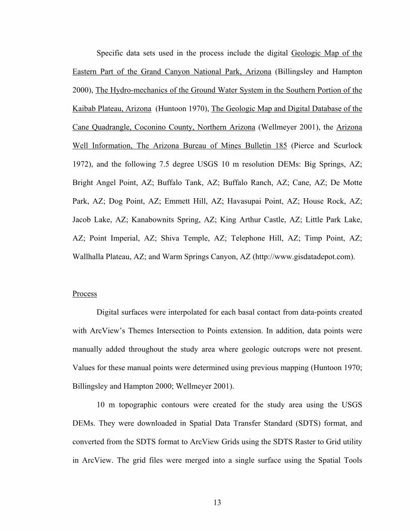
The new contact elevation point shapefile had an extremely random point
distribution, with closely spaced points along the rim of Grand Canyon and no points in
the northern two-thirds of the study area. For improved surface interpolation, points were
manually added along Roaring Springs graben and throughout the northern two-thirds of
the study area. One oil exploration well is located near the northern boundary of the study
15
area, providing known contact elevations at that location (Scurlock 1973). Data points
along Roaring Springs graben were assigned values based on calculations of strike and
dip. Data points throughout the northern study area were assigned values based on
previous geologic maps (Figure 2).
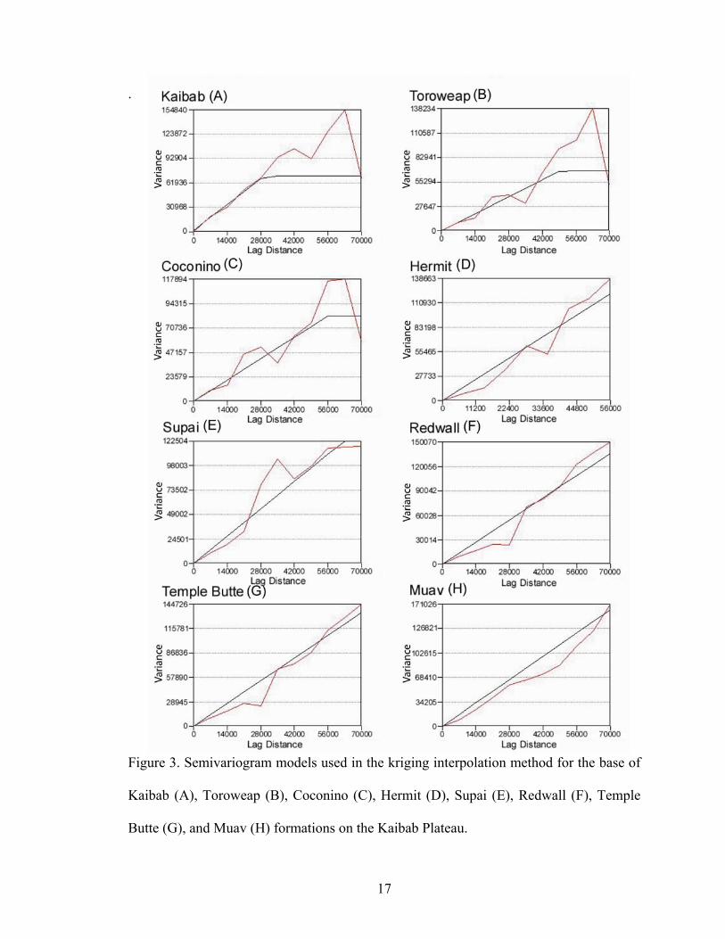
The lower contact surface of each geologic unit was interpolated using ArcView’s
Spatial Tools 3.4 extension. Ordinary kriging using a linear (with sill) semivariogram
model was chosen as the interpolation method for these geologic datasets. The
semivariogram model characterizes the spatial continuity of basal contact elevation for
pairs of locations as a function of the distance between the locations (lag). The model fit
is affected by the choice of lag interval. The data point spacing in the northern study area
determines a lag interval of 7,000 m. The irregularity of each geologic surface results in a
different ‘best fit’ model for each layer. Because 75% of the geologic surfaces were best
fit with the linear (with sill) model (Figure 3), this is the model used to interpolate all the
surfaces. The interpolated surfaces have a uniform grid cell size of 20 meters2. A variable
search radius of 30,000 m was defined and 12 data points were chosen for grid
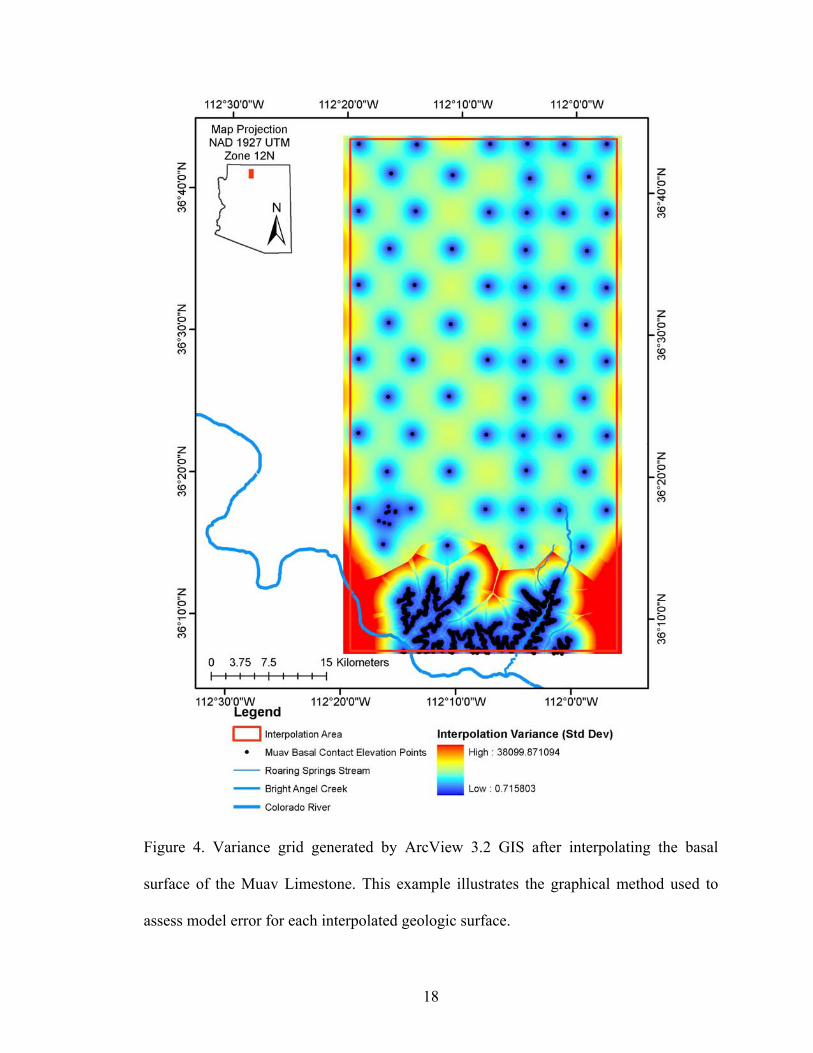
interpolation. An analysis of the model fit was accomplished through the use of the
variance grid, which highlights how accurate the estimated values are and provides
evidence of problems of the fit (Figure 4).
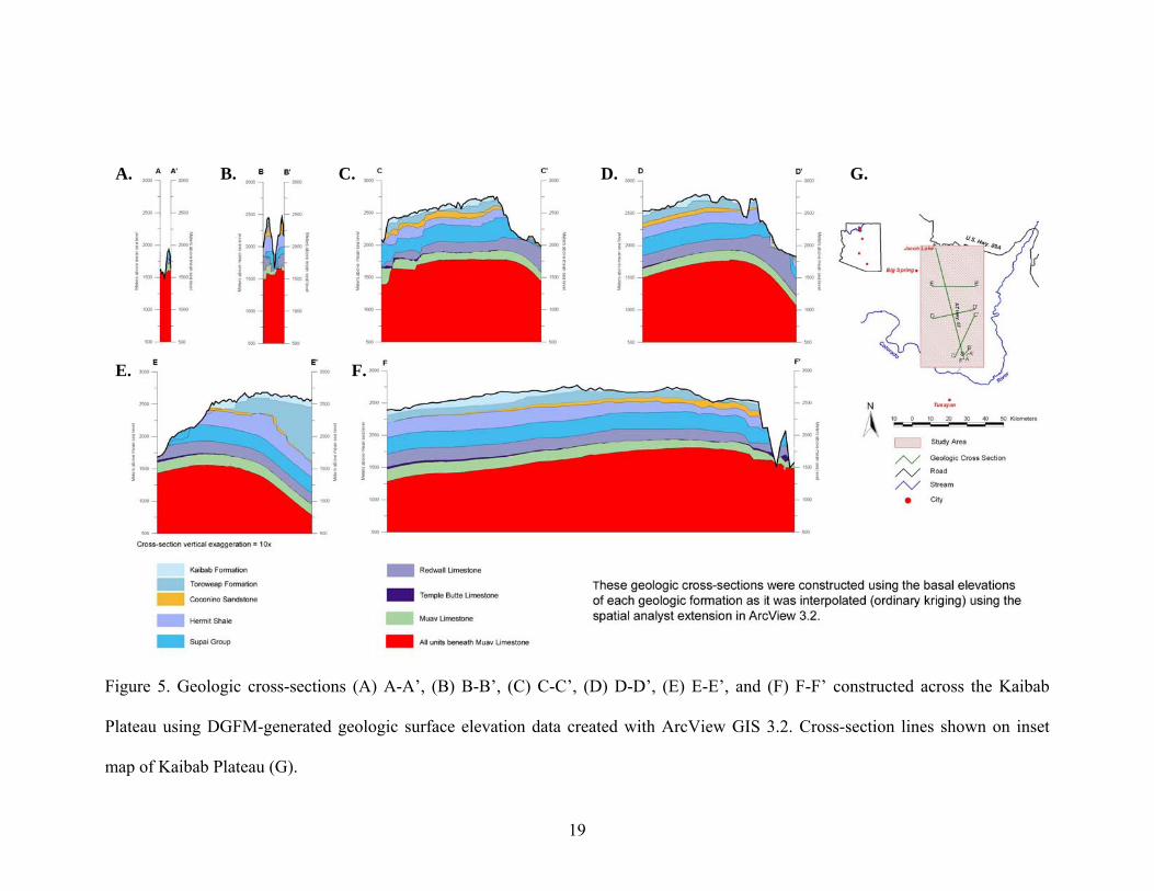
The model fit was also assessed by creating geologic cross-sections using the
interpolated surfaces (Figure 5). Geologic unit profiles were created using the Spatial
Tools 3.4 extension. Each geologic unit cross section profile was exported as a *.txt file,
and then opened and graphed in Microsoft Excel. These cross-sections illustrate the
DGFM’s ability to represent structural topography on the Kaibab Plateau.
16
Figure 2. Basal geologic contact elevation data point distribution for the Kaibab and
Muav formations. This figure illustrates the range in geologic contact elevation data set
variability. Base map modified from Billingsley and Hampton (2000).
17
.
Figure 3. Semivariogram models used in the kriging interpolation method for the base of
Kaibab (A), Toroweap (B), Coconino (C), Hermit (D), Supai (E), Redwall (F), Temple
Butte (G), and Muav (H) formations on the Kaibab Plateau.
18
Figure 4. Variance grid generated by ArcView 3.2 GIS after interpolating the basal
surface of the Muav Limestone. This example illustrates the graphical method used to
assess model error for each interpolated geologic surface.
19
Figure 5. Geologic cross-sections (A) A-A’, (B) B-B’, (C) C-C’, (D) D-D’, (E) E-E’, and (F) F-F’ constructed across the Kaibab
Plateau using DGFM-generated geologic surface elevation data created with ArcView GIS 3.2. Cross-section lines shown on inset
map of Kaibab Plateau (G).
A.
E. F.
B. C. D. G.
20
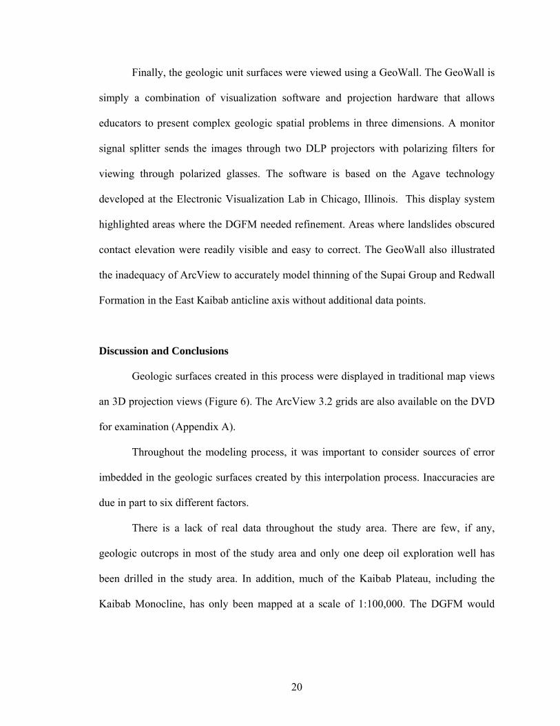
Finally, the geologic unit surfaces were viewed using a GeoWall. The GeoWall is
simply a combination of visualization software and projection hardware that allows
educators to present complex geologic spatial problems in three dimensions. A monitor
signal splitter sends the images through two DLP projectors with polarizing filters for
viewing through polarized glasses. The software is based on the Agave technology
developed at the Electronic Visualization Lab in Chicago, Illinois. This display system
highlighted areas where the DGFM needed refinement. Areas where landslides obscured
contact elevation were readily visible and easy to correct. The GeoWall also illustrated
the inadequacy of ArcView to accurately model thinning of the Supai Group and Redwall
Formation in the East Kaibab anticline axis without additional data points.
Discussion and Conclusions
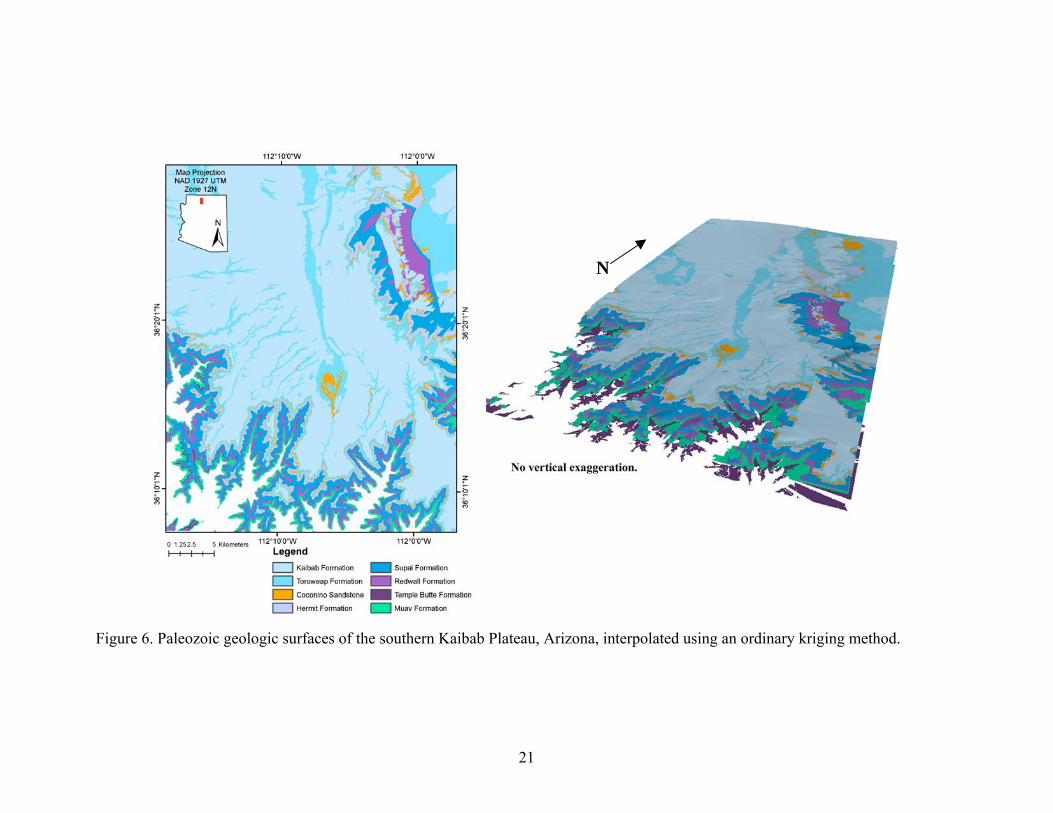
Geologic surfaces created in this process were displayed in traditional map views
an 3D projection views (Figure 6). The ArcView 3.2 grids are also available on the DVD
for examination (Appendix A).
Throughout the modeling process, it was important to consider sources of error
imbedded in the geologic surfaces created by this interpolation process. Inaccuracies are
due in part to six different factors.
There is a lack of real data throughout the study area. There are few, if any,
geologic outcrops in most of the study area and only one deep oil exploration well has
been drilled in the study area. In addition, much of the Kaibab Plateau, including the
Kaibab Monocline, has only been mapped at a scale of 1:100,000. The DGFM would
21
Figure 6. Paleozoic geologic surfaces of the southern Kaibab Plateau, Arizona, interpolated using an ordinary kriging method.
N
22
benefit from 1:24,000 scale mapping along the entire length of the monocline, where
there are some inaccuracies in the interpolated thicknesses of some geologic units.
Multiple data sources affect data accuracy, in part due to differing map scales.
The effect of map scale on spatial data accuracy is particularly apparent when examining
geologic contact locations. In many places, contacts do not accurately follow mapped
topographic contours. Instead, contacts cross many contour lines, suggesting a false sense
of strike and dip in some locations. The interpolation process, which averages
neighboring data points, addresses much of this problem. It is an important concept to
keep in mind, however. The resulting geologic surfaces should not be used for
quantitative analysis at a scale less than 1:100,000.
The random distribution of data points affected the interpolation process. Along
the rim of Grand Canyon, contact elevation data points are aligned in rows. This may
lead to a directional bias in the interpolation. Kriging was the interpolation method
chosen because it historically handles irregular data better than the inverse-distance-
weighted (IDW) or the spline method (Wingle 1992; Zimmerman et al 1999; Siska and I-
Kuai 2001). Future improved interpolation methods may improve this model.
ArcView is unable to interpolate a surface that folds over itself. Only one
elevation value is allowed for each point in x-y space; the highest surface of overturned
geologic units is identified. The model fit along the East Kaibab Monocline, therefore, is
not accurate. The modeled eastern flank of the axis does not dip steeply enough, and it
does not reflect the thinning of geologic units such as the Supai Formation and Redwall
Limestone (Huntoon 1970; Tindall 2000a, b). There is no way to correct this problem
23
using ArcView software, because the software lacks the ability to create overturned beds
like those found in the monocline axis.
The effect of geologic processes such as landslides and high-angle gravity faults
complicates the accurate identification of geologic contact elevations. The modeled
surfaces “stair-step” from the north down to the Canyon’s rim. Large blocks appear to be
sliding off the side of the Kaibab Plateau and into Grand Canyon. While this appearance
is partially an artifact of the interpolation process, it is also due to the fact that landslides
and faulting along the Canyon walls have caused blocks to rotate and have buried
contacts in some places (Hereford and Huntoon 1990). In addition, extensional tectonics
created small grabens and other structures that have not been mapped but that affect
geologic contact elevations. The ability of the interpolation process to identify these
gravity faults was an unexpected and interesting outcome.
After considering the DGFM limitations, the model is deemed appropriate for use
in the larger groundwater flow modeling effort at Roaring Springs. The primary purposes
of the DGFM are to 1) provide general aquifer geometry; small scale variability will not
be preserved in subsequent numerical groundwater flow modeling, and 2) highlight
probable groundwater flow boundaries such as structural highs and lows that will control
the direction of groundwater flow to Roaring Springs. The DGFM succeeds at these two
primary goals. DGFM datasets are also compatible with a GeoWall system for
educational presentations to highlight the structural controls on the hydrogeologic system
of the Kaibab Plateau (Ross 2003; Fry and Springer 2005a, b).
24
CHAPTER 3
CONCEPTUAL GROUNDWATER FLOW MODEL
Purpose and Objectives
A conceptual model was constructed to organize the field data for the Roaring
Springs groundwater flow system. The objectives were to define the groundwater flow
model boundaries, define the hydrostratigraphic units, create a conceptual water budget,
and define the groundwater flow system.
Data Collection Methodology
Data to support a water budget for Roaring Springs are sparse (Johnson and
Sanderson 1968; Huntoon 1970; Rihs 2002). Precipitation data at Bright Angel Ranger
Station, approximately two kilometers from Roaring Springs, are adequate. However,
only seven discharge measurements exist for Roaring Springs between 1952 and 1994
(Johnson and Sanderson 1968; Huntoon 1970; Bills and Flynn 2002); many of these
measurements were actually made some distance downstream from the springs. It was a
goal of this study to collect additional field data that would highlight the seasonal
variability of flow through the R-aquifer. Spring discharge and isotope data were
collected from March through October of 2003 (Appendix B). This included the period of
spring recharge due to snowmelt and the monsoon season.
Aquifer hydraulic head and discharge were measured at three locations in Roaring
Springs canyon: upstream of Roaring Springs where small but perennial flow occurs,
immediately downstream of the Roaring Springs complex, and in Roaring Springs cave
25
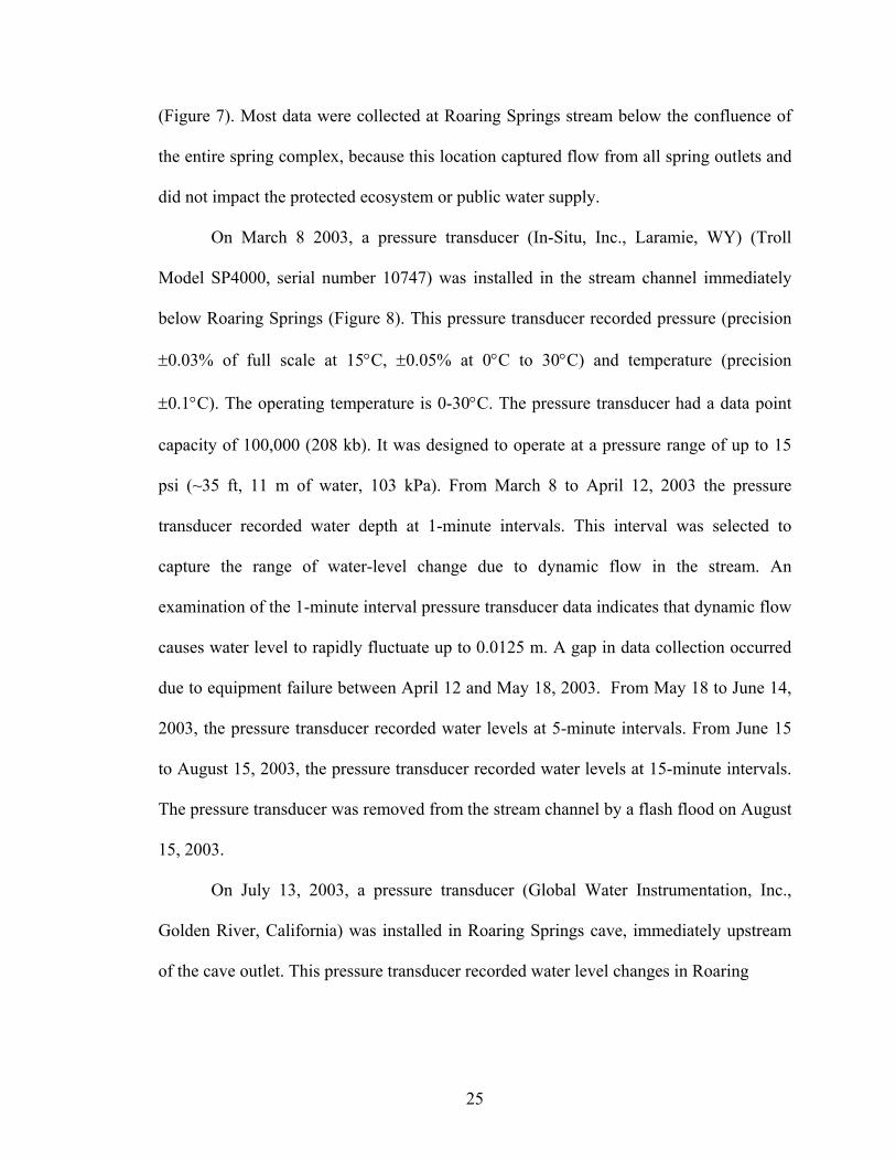
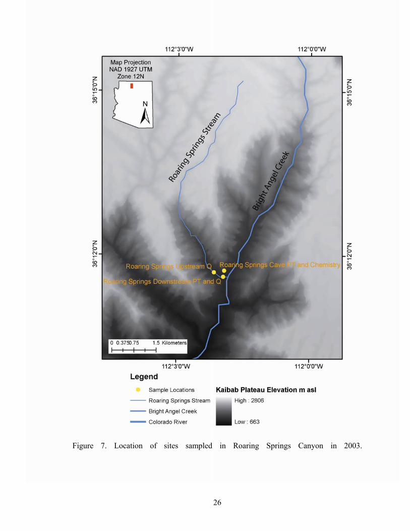
(Figure 7). Most data were collected at Roaring Springs stream below the confluence of
the entire spring complex, because this location captured flow from all spring outlets and
did not impact the protected ecosystem or public water supply.
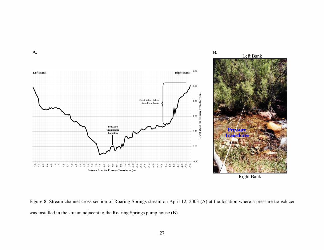
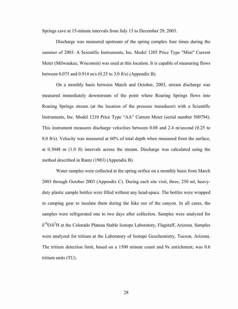
On March 8 2003, a pressure transducer (In-Situ, Inc., Laramie, WY) (Troll
Model SP4000, serial number 10747) was installed in the stream channel immediately
below Roaring Springs (Figure 8). This pressure transducer recorded pressure (precision
±0.03% of full scale at 15°C, ±0.05% at 0°C to 30°C) and temperature (precision
±0.1°C). The operating temperature is 0-30°C. The pressure transducer had a data point
capacity of 100,000 (208 kb). It was designed to operate at a pressure range of up to 15
psi (~35 ft, 11 m of water, 103 kPa). From March 8 to April 12, 2003 the pressure
transducer recorded water depth at 1-minute intervals. This interval was selected to
capture the range of water-level change due to dynamic flow in the stream. An
examination of the 1-minute interval pressure transducer data indicates that dynamic flow
causes water level to rapidly fluctuate up to 0.0125 m. A gap in data collection occurred
due to equipment failure between April 12 and May 18, 2003. From May 18 to June 14,
2003, the pressure transducer recorded water levels at 5-minute intervals. From June 15
to August 15, 2003, the pressure transducer recorded water levels at 15-minute intervals.
The pressure transducer was removed from the stream channel by a flash flood on August
15, 2003.
On July 13, 2003, a pressure transducer (Global Water Instrumentation, Inc.,
Golden River, California) was installed in Roaring Springs cave, immediately upstream
of the cave outlet. This pressure transducer recorded water level changes in Roaring
26
Figure 7. Location of sites sampled in Roaring Springs Canyon in 2003.
27
Figure 8. Stream channel cross section of Roaring Springs stream on April 12, 2003 (A) at the location where a pressure transducer
was installed in the stream adjacent to the Roaring Springs pump house (B).
Roaring Springs Stream Channel Cross Section at Pressure TransducerApril 12, 2003
-0.50
0.00
0.50
1.00
1.50
2.00
2.50
-7.6
-7.2
-6.8
-6.4
-6.0
-5.6
-5.2
-4.8
-4.4
-4.0
-3.6
-3.2
-2.8
-2.4
-2.0
-1.6
-1.2
-0.8
-0.40.0
0.4
0.8
1.2
1.6
2.0
2.4
2.8
3.2
3.6
4.0
4.4
4.8
5.2
5.6
6.0
6.4
6.8
7.2
7.6
Distance from the Pressure Transducer (m)
Hei
ght a
bove
the
Pres
sure
Tra
nsdu
cer
(m)
Left Bank Right Bank
Pressure Transducer
Location
Construction debrisfrom Pumphouse
Pressure Transducer
Right Bank
Left BankA. B.
28
Springs cave at 15-minute intervals from July 13 to December 29, 2003.
Discharge was measured upstream of the spring complex four times during the
summer of 2003. A Scientific Instruments, Inc. Model 1205 Price Type "Mini" Current
Meter (Milwaukee, Wisconsin) was used at this location. It is capable of measuring flows
between 0.075 and 0.914 m/s (0.25 to 3.0 ft/s) (Appendix B).
On a monthly basis between March and October, 2003, stream discharge was
measured immediately downstream of the point where Roaring Springs flows into
Roaring Springs stream (at the location of the pressure transducer) with a Scientific
Instruments, Inc. Model 1210 Price Type “AA” Current Meter (serial number 500794).
This instrument measures discharge velocities between 0.08 and 2.4 m/second (0.25 to
8.0 ft/s). Velocity was measured at 60% of total depth when measured from the surface,
at 0.3048 m (1.0 ft) intervals across the stream. Discharge was calculated using the
method described in Rantz (1983) (Appendix B).
Water samples were collected at the spring orifice on a monthly basis from March
2003 through October 2003 (Appendix C). During each site visit, three, 250 ml, heavy-
duty plastic sample bottles were filled without any head-space. The bottles were wrapped
in camping gear to insulate them during the hike out of the canyon. In all cases, the
samples were refrigerated one to two days after collection. Samples were analyzed for
δ18O/δ2H at the Colorado Plateau Stable Isotope Laboratory, Flagstaff, Arizona. Samples
were analyzed for tritium at the Laboratory of Isotope Geochemistry, Tucson, Arizona.
The tritium detection limit, based on a 1500 minute count and 9x enrichment, was 0.6
tritium units (TU).
29
The pH and specific conductance of the spring water were measured during
monthly site visits (Appendix C). The pH-temperature probe used was an Orion Model
250A (Beverley, Massachusetts) (serial number 004927). The specific conductance probe
was an Orion Model 122 (serial number 24020099). The pH probe was calibrated with
pH 7 and 10 buffers on the day the spring was sampled.
Conceptual Model Boundaries
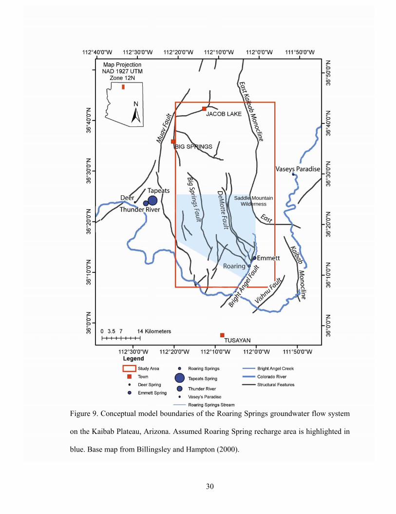
The study area is on the southern Kaibab Plateau which is defined by the
geometry of the East Kaibab Monocline (Figure 9). The aerial extent of the groundwater
flow system supplying water to Roaring Springs is truncated on the south by Grand
Canyon. The axis of the East Kaibab monocline, north and east of Roaring Springs, is a
likely groundwater divide. The western boundary of the groundwater flow system is
uncertain but likely does not extend beyond the Muav fault. The northern boundary of the
groundwater flow system is also uncertain; a groundwater divide may be present at the
crest of the Kaibab Plateau in the Saddle Mountain Wilderness, from which stratigraphy
dips gently to the north and south. Depending on the elevation of the potentiometric
surface of the aquifer, the groundwater flow system may continue north past the Arizona-
Utah border.
Hydrostratigraphic Units
The hydraulic properties of the aquifers in the study area are controlled by the
bedrock lithology, subsequent structural deformation of the bedrock, and ongoing
chemical processes such as carbonate dissolution along fractures.
30
Figure 9. Conceptual model boundaries of the Roaring Springs groundwater flow system
on the Kaibab Plateau, Arizona. Assumed Roaring Spring recharge area is highlighted in
blue. Base map from Billingsley and Hampton (2000).
Saddle Mountain Wilderness
31
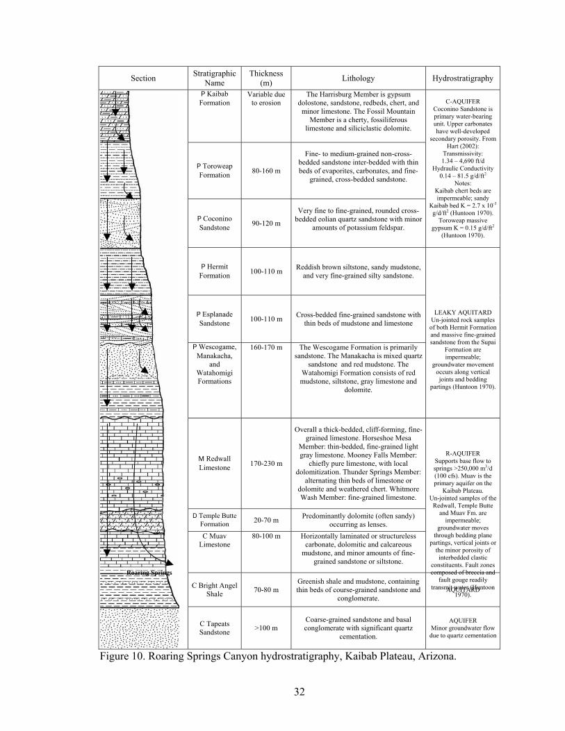
The R-aquifer, which is the focus of the study, discharges through large karst
springs on the North Rim of Grand Canyon. It is composed of three geologic units: the
Muav Formation, the Temple Butte Formation, and the Redwall Formation (Figure 10).
Due to their similar hydrogeologic properties, they are grouped as one hydrostratigraphic
unit in the conceptual model. The Bright Angel Shale forms a barrier to flow at the base
of the aquifer, although this boundary is variable due to a complex relationship with the
Muav Formation. Overall, the thickness of the aquifer is ~400 m, although it gradually
thickens to the west (Huntoon 1970; Middleton and Elliot 1990). A conceptual
understanding of flow through the R-aquifer also relies on the hydrogeologic properties
of the rock units above and below it. The Paleozoic stratigraphy and structural evolution
of Grand Canyon has been studied in great detail by many researchers over many
decades. The following discussion attempts to place the study area in its proper geologic
context and to highlight stratigraphic and structural details that have a specific bearing on
groundwater movement through the section.
Stratigraphy
The stratigraphy of the Kaibab Plateau is well exposed in Grand Canyon. Highly
metamorphosed Proterozoic basement and the Grand Canyon Supergroup are overlain by
relatively unaltered sedimentary sequences of sandstone, limestone, and shale. The
limestone formations show evidence of dissolution enhancement beginning soon after
their formation and continuing in cycles until the present day. Quaternary deposits of
alluvium and colluvium discontinuously cover the Plateau (Huntoon 2000).
32
Section Stratigraphic Name
Thickness (m) Lithology Hydrostratigraphy
P Kaibab Formation
Variable due to erosion
The Harrisburg Member is gypsum dolostone, sandstone, redbeds, chert, and
minor limestone. The Fossil Mountain Member is a cherty, fossiliferous
limestone and siliciclastic dolomite.
P Toroweap Formation 80-160 m
Fine- to medium-grained non-cross-bedded sandstone inter-bedded with thin beds of evaporites, carbonates, and fine-
grained, cross-bedded sandstone.
P Coconino Sandstone 90-120 m
Very fine to fine-grained, rounded cross-bedded eolian quartz sandstone with minor
amounts of potassium feldspar.
C-AQUIFER Coconino Sandstone is primary water-bearing unit. Upper carbonates have well-developed
secondary porosity. From Hart (2002):
Transmissivity: 1.34 – 4,690 ft/d
Hydraulic Conductivity 0.14 – 81.5 g/d/ft2
Notes: Kaibab chert beds are impermeable; sandy
Kaibab bed K = 2.7 x 10⁻³ g/d/ft2 (Huntoon 1970).
Toroweap massive gypsum K = 0.15 g/d/ft2
(Huntoon 1970).
P Hermit Formation 100-110 m Reddish brown siltstone, sandy mudstone,
and very fine-grained silty sandstone.
P Esplanade Sandstone 100-110 m Cross-bedded fine-grained sandstone with
thin beds of mudstone and limestone
P Wescogame, Manakacha,
and Watahomigi Formations
160-170 m The Wescogame Formation is primarily sandstone. The Manakacha is mixed quartz
sandstone and red mudstone. The Watahomigi Formation consists of red mudstone, siltstone, gray limestone and
dolomite.
LEAKY AQUITARD Un-jointed rock samples
of both Hermit Formation and massive fine-grained sandstone from the Supai
Formation are impermeable;
groundwater movement occurs along vertical joints and bedding
partings (Huntoon 1970).
M Redwall Limestone 170-230 m
Overall a thick-bedded, cliff-forming, fine-grained limestone. Horseshoe Mesa
Member: thin-bedded, fine-grained light gray limestone. Mooney Falls Member:
chiefly pure limestone, with local dolomitization. Thunder Springs Member:
alternating thin beds of limestone or dolomite and weathered chert. Whitmore Wash Member: fine-grained limestone.
D Temple Butte Formation 20-70 m Predominantly dolomite (often sandy)
occurring as lenses. C Muav
Limestone 80-100 m Horizontally laminated or structureless
carbonate, dolomitic and calcareous mudstone, and minor amounts of fine-
grained sandstone or siltstone.
R-AQUIFER Supports base flow to springs >250,000 m3/d (100 cfs). Muav is the primary aquifer on the
Kaibab Plateau. Un-jointed samples of the
Redwall, Temple Butte and Muav Fm. are
impermeable; groundwater moves
through bedding plane partings, vertical joints or
the minor porosity of interbedded clastic
constituents. Fault zones composed of breccia and
fault gouge readily transmit water (Huntoon
1970).
C Bright Angel
Shale 70-80 m Greenish shale and mudstone, containing thin beds of course-grained sandstone and
conglomerate. AQUITARD
C Tapeats Sandstone >100 m
Coarse-grained sandstone and basal conglomerate with significant quartz
cementation.
AQUIFER Minor groundwater flow due to quartz cementation
Figure 10. Roaring Springs Canyon hydrostratigraphy, Kaibab Plateau, Arizona.
Roaring Springs

33
Bright Angel Shale
In Roaring Springs Canyon, the Bright Angel Shale is approximately 100 m thick,
but this thickness varies considerably due to intertonguing with the overlying Muav
Formation. Shale, composed mostly of illitic clay and smaller amounts of chlorite and
kaolinite, is the primary lithology. Beds of fine-grained sandstone and siltstone are also
present (Middleton and Elliot 1990). Bed thickness ranges from a few centimeters to
approximately 5 m on the eastern Kaibab Plateau (Huntoon 1970). The dramatic red,
purple, and green colors in this unit are due to the presence of iron oxide cement,
hematitic ooids and glauconite. The high clay content of the Bright Angel Shale allows it
to hydrologically seal faults when the shale is pulverized to an impermeable gouge; open
(hydrologically active) fractures are uncommon (Huntoon 1970). In Grand Canyon, most
springs in the lower Paleozoic section discharge above the Bright Angel Shale. The
depositional environment of the Bright Angel Shale is interpreted to be a subtidal
environment affected by long-term movements of the strandline (Middleton and Elliot
1990). This environmental variation is recorded in the irregular surface topography,
lithology and sedimentary structures of the Bright Angel Shale. The direction and rate of
groundwater flow through this unit is a function of all of these components, but the
surface topography, in particular, is an important control on groundwater flow direction
through the overlying R-aquifer. Surface topography has been dramatically affected by
the structural development of the Kaibab Plateau, as illustrated by the DGFM.
34
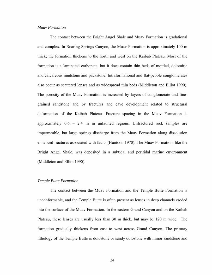
Muav Formation
The contact between the Bright Angel Shale and Muav Formation is gradational
and complex. In Roaring Springs Canyon, the Muav Formation is approximately 100 m
thick; the formation thickens to the north and west on the Kaibab Plateau. Most of the
formation is a laminated carbonate, but it does contain thin beds of mottled, dolomitic
and calcareous mudstone and packstone. Intraformational and flat-pebble conglomerates
also occur as scattered lenses and as widespread thin beds (Middleton and Elliot 1990).
The porosity of the Muav Formation is increased by layers of conglomerate and fine-
grained sandstone and by fractures and cave development related to structural
deformation of the Kaibab Plateau. Fracture spacing in the Muav Formation is
approximately 0.6 – 2.4 m in unfaulted regions. Unfractured rock samples are
impermeable, but large springs discharge from the Muav Formation along dissolution
enhanced fractures associated with faults (Huntoon 1970). The Muav Formation, like the
Bright Angel Shale, was deposited in a subtidal and peritidal marine environment
(Middleton and Elliot 1990).
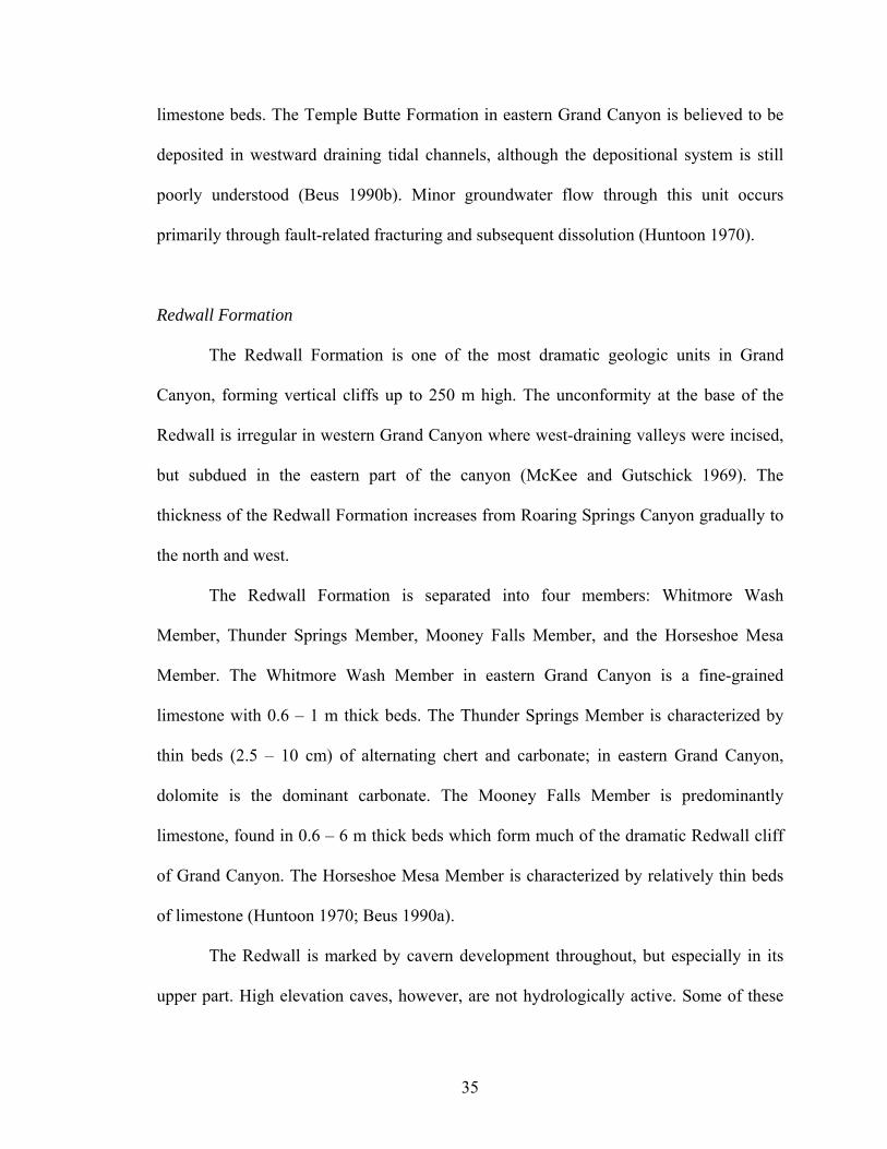
Temple Butte Formation
The contact between the Muav Formation and the Temple Butte Formation is
unconformable, and the Temple Butte is often present as lenses in deep channels eroded
into the surface of the Muav Formation. In the eastern Grand Canyon and on the Kaibab
Plateau, these lenses are usually less than 30 m thick, but may be 120 m wide. The
formation gradually thickens from east to west across Grand Canyon. The primary
lithology of the Temple Butte is dolostone or sandy dolostone with minor sandstone and
35
limestone beds. The Temple Butte Formation in eastern Grand Canyon is believed to be
deposited in westward draining tidal channels, although the depositional system is still
poorly understood (Beus 1990b). Minor groundwater flow through this unit occurs
primarily through fault-related fracturing and subsequent dissolution (Huntoon 1970).
Redwall Formation
The Redwall Formation is one of the most dramatic geologic units in Grand
Canyon, forming vertical cliffs up to 250 m high. The unconformity at the base of the
Redwall is irregular in western Grand Canyon where west-draining valleys were incised,
but subdued in the eastern part of the canyon (McKee and Gutschick 1969). The
thickness of the Redwall Formation increases from Roaring Springs Canyon gradually to
the north and west.
The Redwall Formation is separated into four members: Whitmore Wash
Member, Thunder Springs Member, Mooney Falls Member, and the Horseshoe Mesa
Member. The Whitmore Wash Member in eastern Grand Canyon is a fine-grained
limestone with 0.6 – 1 m thick beds. The Thunder Springs Member is characterized by
thin beds (2.5 – 10 cm) of alternating chert and carbonate; in eastern Grand Canyon,
dolomite is the dominant carbonate. The Mooney Falls Member is predominantly
limestone, found in 0.6 – 6 m thick beds which form much of the dramatic Redwall cliff
of Grand Canyon. The Horseshoe Mesa Member is characterized by relatively thin beds
of limestone (Huntoon 1970; Beus 1990a).
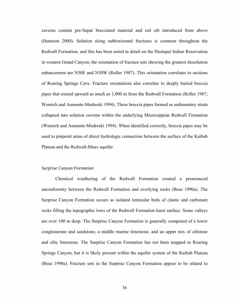
The Redwall is marked by cavern development throughout, but especially in its
upper part. High elevation caves, however, are not hydrologically active. Some of these
36
caverns contain pre-Supai brecciated material and red silt introduced from above
(Huntoon 2000). Solution along subhorizontal fractures is common throughout the
Redwall Formation, and this has been noted in detail on the Hualapai Indian Reservation
in western Grand Canyon; the orientation of fracture sets showing the greatest dissolution
enhancement are N50E and N50W (Roller 1987). This orientation correlates to sections
of Roaring Springs Cave. Fracture orientations also correlate to deeply buried breccia
pipes that extend upward as much as 1,000 m from the Redwall Formation (Roller 1987;
Wenrich and Aumente-Modreski 1994). These breccia pipes formed as sedimentary strata
collapsed into solution caverns within the underlying Mississippian Redwall Formation
(Wenrich and Aumente-Modreski 1994). When identified correctly, breccia pipes may be
used to pinpoint areas of direct hydrologic connection between the surface of the Kaibab
Plateau and the Redwall-Muav aquifer.
Surprise Canyon Formation
Chemical weathering of the Redwall Formation created a pronounced
unconformity between the Redwall Formation and overlying rocks (Beus 1990a). The
Surprise Canyon Formation occurs as isolated lenticular beds of clastic and carbonate
rocks filling the topographic lows of the Redwall Formation karst surface. Some valleys
are over 100 m deep. The Surprise Canyon Formation is generally composed of a lower
conglomerate and sandstone, a middle marine limestone, and an upper mix of siltstone
and silty limestone. The Surprise Canyon Formation has not been mapped in Roaring
Springs Canyon, but it is likely present within the aquifer system of the Kaibab Plateau
(Beus 1990a). Fracture sets in the Surprise Canyon Formation appear to be related to
37
fractures in the Redwall Formation below, particularly in the basal conglomerate (Roller
1987). The depositional environment of the Surprise Canyon Formation is fluvial,
grading into a marine environment.
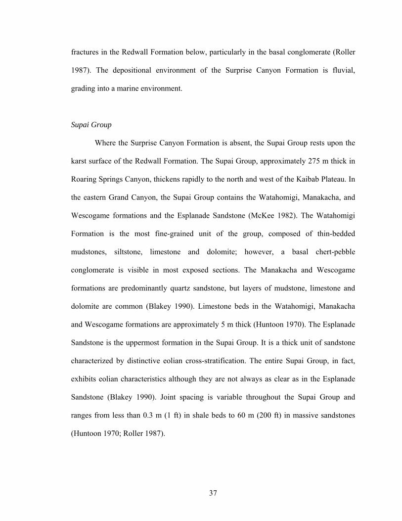
Supai Group
Where the Surprise Canyon Formation is absent, the Supai Group rests upon the
karst surface of the Redwall Formation. The Supai Group, approximately 275 m thick in
Roaring Springs Canyon, thickens rapidly to the north and west of the Kaibab Plateau. In
the eastern Grand Canyon, the Supai Group contains the Watahomigi, Manakacha, and
Wescogame formations and the Esplanade Sandstone (McKee 1982). The Watahomigi
Formation is the most fine-grained unit of the group, composed of thin-bedded
mudstones, siltstone, limestone and dolomite; however, a basal chert-pebble
conglomerate is visible in most exposed sections. The Manakacha and Wescogame
formations are predominantly quartz sandstone, but layers of mudstone, limestone and
dolomite are common (Blakey 1990). Limestone beds in the Watahomigi, Manakacha
and Wescogame formations are approximately 5 m thick (Huntoon 1970). The Esplanade
Sandstone is the uppermost formation in the Supai Group. It is a thick unit of sandstone
characterized by distinctive eolian cross-stratification. The entire Supai Group, in fact,
exhibits eolian characteristics although they are not always as clear as in the Esplanade
Sandstone (Blakey 1990). Joint spacing is variable throughout the Supai Group and
ranges from less than 0.3 m (1 ft) in shale beds to 60 m (200 ft) in massive sandstones
(Huntoon 1970; Roller 1987).
38
The depositional environment of the Supai Group is understood to be a coastal
plain affected by fluctuations in sea level – leading to a complex combination of eolian
and noneolian carbonate sandstones, red siltstone and mudstone, and local conglomerate
(Blakey 1990). Groundwater flow through such a unit is equally complex. A significant
amount of water in this unit moves relatively slowly down through sand bodies until a
layer of mudstone forces the water to flow horizontally to the Canyon walls. Some water
flows rapidly down through well-developed joints in the Supai Group (Huntoon 1970).
Evidence of these complex flow paths can be seen in the small perched aquifers and
springs that swell during the late winter and spring and wane during the dry summer.
Hermit Formation
The Hermit Formation is approximately 100 m thick in Roaring Springs Canyon.
This formation thickens dramatically across Grand Canyon from east to west. It is
primarily a silty sandstone or sandy mudstone. Intraformational conglomerates are
common. In general, sandstone is more abundant at the base of the formation, and
mudstone increases upward. Cracks at the top of this formation can reach over 5 meters
depth, and are filled with sandstone of the Coconino Formation (Blakey 1990).
Structureless units form beds 1 m thick. Vertically continuous joints are spaced at greater
than 0.3 m. Unfractured rock samples are impermeable when tested in the laboratory
(Huntoon 1970). Complex cross-bedding is common and indicative of a fluvial
depositional environment (Blakey 1990). Like the underlying Supai, the Hermit Shale
acts as a regional aquitard where it is unfaulted (Huntoon 1970).
39
Coconino Sandstone
The tall white cliffs of the Coconino Sandstone are one of the most obvious
features in Grand Canyon. The Coconino Sandstone is approximately 100 m thick in
Roaring Springs Canyon, and it thins to the north. The northern edge of deposition on the
Kaibab Plateau roughly correlates to the Arizona-Utah border (Blakey 1990). The
Coconino is a homogenous, fine- to medium-grained, complexly cross-bedded quartz
sandstone. Crossbed sets range from 1.5 – 23 m thick. The Coconino Sandstone is in
many ways an ideal aquifer, and supplies water to communities across northern Arizona
(Hart et al 2002a; Bills and Flynn 2002). On the Kaibab Plateau, it acts as a perched
aquifer where the underlying Hermit Shale is unfaulted. Numerous small springs and a
large spring, Big Spring, issue from the Coconino where a fault has uplifted and exposed
the sandstone on the North Rim (Huntoon 1970). The Coconino Sandstone was deposited
as large dunes advanced across the landscape. Dune morphology and migration was
controlled by regional structural features (primarily the Sedona Arch), resulting in
variable unit thickness across Arizona (Blakey 1990).
Toroweap Formation
In the Marble Canyon area, the fine- to medium-grained sandstones of the
Toroweap Formation intertongue with the Coconino Sandstone. The Toroweap
Formation is approximately 120 m thick in Roaring Springs Canyon; it pinches out
entirely to the east of Grand Canyon. Significant vertical heterogeneity is present. The
formation is made up of three members: the Woods Ranch Member is an upper evaporite
and redbed interval, the Brady Canyon Member is a middle limestone unit, and the
40
Seligman Member is a lower sandstone and evaporite interval. Evaporite facies are
predominantly found north of Grand Canyon (Turner 1990). Joint spacing in the
Toroweap ranges from 0.05 – 1 m in redbeds to 2.5 m in limestone beds. This is a
complex hydrogeologic setting, with multiple groundwater flow pathways. These
pathways have been enhanced through karst development where the formation outcrops
on the surface of the Kaibab Plateau (Huntoon 1970).
Springs are common in the Toroweap Formation where clastic layers prohibit
vertical migration of infiltrating groundwater. Laboratory analyses of unfractured
Toroweap limestone indicate that this rock is impermeable; gypsum samples yielded a
permeability of 6.1 x 10⁻³ m/d (Huntoon 1970).
The depositional setting of this formation was a fluctuating shallow marine
environment, tidal flats, sabkhas, and eolian dune fields. The shoreline was commonly in
the vicinity of Grand Canyon, leading to the dramatic changes in lithofacies in the
Canyon (Turner 1990).
Kaibab Formation
The Kaibab Formation is the uppermost geologic unit on the Kaibab Plateau. Its
thickness in Roaring Springs Canyon is variable due to erosion, which obscures its
original geometry. This unit gradually thickens to the west. The base of the Kaibab
Formation, a cherty carbonate, is underlain by gypsum and the deformed sandstones of
the Toroweap Formation. The contact between the two formations is marked by localized
breccias and erosional surfaces that formed as collapse features related to evaporite
dissolution in the upper Toroweap Formation. The Kaibab Formation is composed of
41
cyclic beds of carbonate and siliciclastic sediments mixed with diagenetic chert and
dolomite (Hopkins 1990).
Two members are recognized: the Fossil Mountain Member consists of
approximately 75% sandstone or sandy dolostone (Hopkins 1990); joint spacing ranges
from 1.2 – 2.4 m (Huntoon 1970). The upper portion of the Kaibab Formation, the
Harrisburg Member, consists of a mix of gypsum, dolostone, sandstone, redbeds, chert,
and minor limestone (Hopkins 1990); joint spacing ranges from 0.05 – 0.61 m (Huntoon
1970). Laboratory analyses of unfractured limestone containing chert from the Kaibab
Formation indicate the rock is impermeable; unfractured sandy limestone has a
permeability of 1.1 x 10⁻⁴ m/d (Huntoon 1970).
The upper surface of the Kaibab Formation is dotted with sinkholes that allow
precipitation to enter the groundwater system. Many small springs have been mapped in
the Kaibab Formation; they are often located at the contact between the Kaibab and
Toroweap Formations but are also found along bedding planes in the Kaibab Formation
(U.S. Forest Service 1994; Billingsley and Hampton 2000). The depositional
environment of the Kaibab Formation was a fluctuating sea level along a mixed
carbonate-siliciclastic ramp (Hopkins 1990).
Structural Geology
The structural history of the Kaibab Plateau is the primary control on groundwater
flow pathways to seeps and springs. The most obvious feature on the Kaibab Plateau is
the East Kaibab monocline. While this structure undoubtedly controls the groundwater
flow system of the Kaibab Plateau, other structural features and events have played an

42
important role in the development of the hydrogeologic character of the region as well.
Structural features affect groundwater flow in two principal ways: direction and
magnitude. Direction is controlled when the aquifer geometry is affected, such as
changing an aquifer’s thickness or slope. Direction can also be controlled by creating
barriers (such as impermeable fault gouge) or conduits (such as fractures). Magnitude can
be controlled by increasing the number, size and connectedness of conduits. Major faults
and folds in the study area include the Bright Angel Fault, Muav Fault, Eminence Fault,
Uncle Jim and DeMotte Faults, Big Springs Fault, and the East Kaibab Monocline
(Figure 11).
The orientation of Precambrian faults (Bright Angel, Butte, Crystal, Muav, and
Phantom-Cremation, for example) is the primary control on the direction of groundwater
flow; these old faults act as “structural hinges” in response to subsequent tectonic events
and changes in sediment loading (Huntoon 1990). Throughout the Paleozoic, minor
movement along these Precambrian faults accommodated the stress created by sediment
loading and distant tectonic events. The effect of this reactivation can be seen in the
variation in thickness of sediments deposited during this time. Huntoon (1990) cited an
example of such variation in a band 400 m wide across the Bright Angel Fault where the
upper 9 m of the Redwall Formation is missing due to reverse motion along the fault.
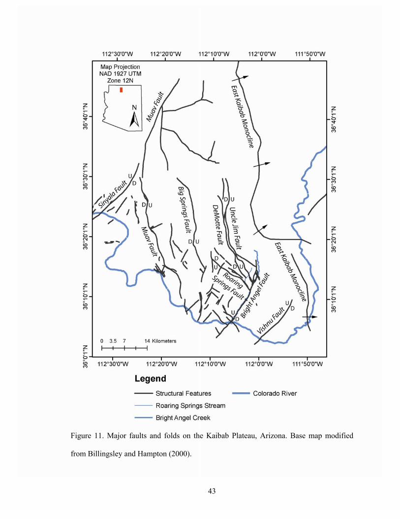
43
Figure 11. Major faults and folds on the Kaibab Plateau, Arizona. Base map modified
from Billingsley and Hampton (2000).
44
Larger faults (greater than 30 m of offset) are associated with fault zones
exceeding 30 m in width and composed of gouge, breccia, and even large blocks torn
from the walls (Huntoon 1970). Shattered rock is found along all fault slip planes. The
fault zones along smaller faults (Roaring Springs Fault, for example) are generally less
than 7 m wide and are composed of gouge and breccia.
The brittle carbonates of the Redwall, Temple Butte, and Muav Formations are
characterized by a regular pattern of fractures associated with faulting. Master joints can
be found spaced at intervals of approximately 300-900 m in a rectilinear network
extending up to 6.5-8 km on each side of major faults. These joints are often enlarged by
dissolution, and are commonly less than 3 m wide but over 15 m high. In eastern Grand
Canyon, joints in the Muav Formation are spaced regularly at intervals of 0.6 - 2 m (2 - 8
ft) in unfaulted regions. Where the Redwall Formation is exposed in the Cockscomb,
many small solution tubes less than 0.5 m in diameter are found (Huntoon 1970). These
faults and associated fractures have increased the permeability of the carbonate and
sandstone units, and dissolution enhancement has enlarged these flow paths (Cepeda
1994). Joint spacing throughout the Paleozoic section is ~1 to 2 times the thickness of the
beds in which they are found (Huntoon 1970).
The tectonic event that has most impacted the shape of the modern Kaibab
Plateau is the Laramide orogeny. The east-northeast crustal shortening that defined this
event led to the development of the Grand Canyon monoclines over preexisting, steeply
west-dipping, Precambrian basement faults (Huntoon 1990). The East Kaibab monocline
is a classic example of Laramide monocline development. After the cessation of
Laramide contraction, the Grand Canyon region was tectonically stable until the onset of
45
east-west extension during the Late Cenozoic. The strain associated with this extension is
accommodated primarily through normal displacement along pre-existing north trending
fault zones. Fracture sets associated with extensional tectonics are particularly likely to
increase the flow rate of groundwater through the bedrock (Huntoon 1990).
The N20E-striking, steeply (60-70°) west dipping Precambrian Butte Fault
underlies the folded Paleozoic and Mesozoic rocks that constitute the east-dipping
Kaibab Monocline fold (Figure 12). This fault was reactivated in a reverse-right-lateral
oblique sense during the Laramide orogeny and it propagated upward through the
stratigraphic section to the level of the Redwall Formation before Laramide deformation
ended (Tindall 2000b). This is common for all the monoclines in Grand Canyon which do
not fault above the Supai (Huntoon 1990). There is ~800 m of offset along the Butte
Fault in Grand Canyon. A sequence of deformation took place along the developing East
Kaibab monocline as Paleozoic and Mesozoic cover rocks folded and faulted in response
to movement on the reactivated basement fault (Tindall 2000b).
In Grand Canyon, thinning and low-grade metamorphism of the lower Paleozoic
rocks occurred in the transition from fault to fold; Huntoon (1990) observed thinning of
the Redwall Formation and Supai Group by 30-60%. Branching is well developed along
the East Kaibab monocline, and prominent northwest-trending branches splay from the
main fold (Tindall 2000a). In addition, segments of the East and West Kaibab monoclines
develop en echelon patterns. Changes in strike and complicated branching of the East
Kaibab monocline are linked on outcrops to intersecting basement fault patterns that have
been reactivated (Huntoon 1990).
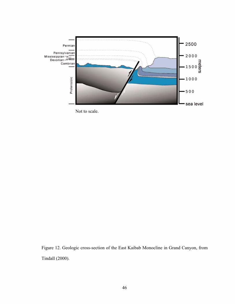
46
Figure 12. Geologic cross-section of the East Kaibab Monocline in Grand Canyon, from
Tindall (2000).
Not to scale.

47
Finally, the surface of the Kaibab Plateau is also criss-crossed by a complex set of
fractures, which can be identified on LandSat imagery. The orientation of this fracture set
shares the same trend as the faults (Gettings and Bultman 2005). In addition, sinkholes in
the Kaibab Limestone appear to correlate with the intersection of these fractures (Cepeda
1994).
Water Budget
A water budget is a volumetric assessment of a groundwater system. Inputs equal
outputs, plus or minus a change in aquifer storage. Inputs to the Roaring Springs
groundwater system are a function of climate, which is controlled by the elevation of the
Kaibab Plateau. Outputs are a function of evapotranspiration, spring discharge, and
through-flow. Downward leakage from the R-aquifer is assumed to be negligible based
on geochemical analysis of springs above and below the Bright Angel Shale which show
very little connection between the two hydrologic systems (Crossey 2002).
The change in storage of this groundwater system is difficult to define, and is
controlled by both inputs and outputs as well as by aquifer characteristics such as aquifer
porosity.
Precipitation
The weather station nearest to Roaring Springs is the Bright Angel Ranger Station
(NOAA COOPID 21001), located at an elevation of 2560.3 meters above sea level (m
asl) on the southern tip of the Kaibab Plateau (Latitude 36: 13:00, Longitude -112:04) in
Coconino County, Arizona. Weather data were collected at this site daily since 1925,

48
although there were some gaps in the record due to the inaccessibility of the site. The
average annual precipitation at this site, based on the 32 years with complete precipitation
records, is 652 mm. January is the wettest month of the year, on average; June is the
driest (http://www4.ncdc.noaa.gov/cgi-win/wwcgi.dll?WWDI~StnSrch). Precipitation
varies with elevation across the Kaibab Plateau, with lower elevations receiving much
less water (Huntoon 1970) (Table 1).
Precipitation occurs in late summer convective thunderstorms and late winter
snowstorms. Summer precipitation is usually a result of thermal heating in Grand
Canyon. Convection cells build through the day and afternoon showers result.
Occasionally, tropical weather patterns will move up through Arizona from the Pacific
Ocean and Gulf of California. In the winter, Pacific storm tracks usually move south and
east into Arizona from the Pacific Northwest and California (Huntoon 1970). These two
different sources of precipitation are associated with different oxygen and hydrogen
stable isotope compositions. Research by Miller (2004) indicates that winter precipitation
on the Kaibab Plateau is characterized by δ18O values of -12.66 %o and δ2H values of -
92.16 %o; summer precipitation is characterized by δ18O values of -6.58 %o and δ2H
values of -40.44 %o.
The precipitation during the 2003 year, when field data were collected for this
study, was 527 mm (94% average). February was the wettest month; June was the driest
(http://www4.ncdc.noaa.gov/cgi-win/wwcgi.dll?WWDI~StnSrch).
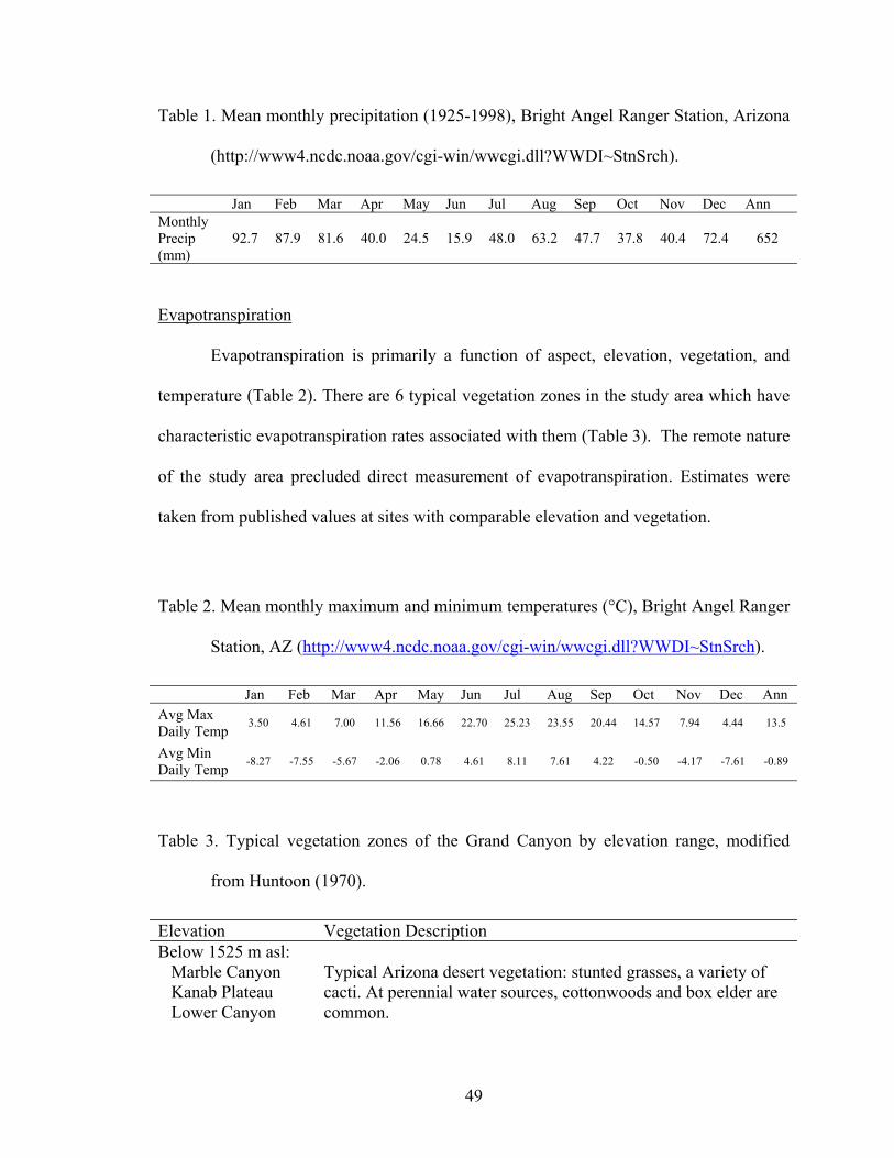
49
Table 1. Mean monthly precipitation (1925-1998), Bright Angel Ranger Station, Arizona
(http://www4.ncdc.noaa.gov/cgi-win/wwcgi.dll?WWDI~StnSrch).
Jan Feb Mar Apr May Jun Jul Aug Sep Oct Nov Dec Ann Monthly Precip (mm)
92.7 87.9 81.6 40.0 24.5 15.9 48.0 63.2 47.7 37.8 40.4 72.4 652
Evapotranspiration
Evapotranspiration is primarily a function of aspect, elevation, vegetation, and
temperature (Table 2). There are 6 typical vegetation zones in the study area which have
characteristic evapotranspiration rates associated with them (Table 3). The remote nature
of the study area precluded direct measurement of evapotranspiration. Estimates were
taken from published values at sites with comparable elevation and vegetation.
Table 2. Mean monthly maximum and minimum temperatures (°C), Bright Angel Ranger
Station, AZ (http://www4.ncdc.noaa.gov/cgi-win/wwcgi.dll?WWDI~StnSrch).
Jan Feb Mar Apr May Jun Jul Aug Sep Oct Nov Dec Ann Avg Max Daily Temp 3.50 4.61 7.00 11.56 16.66 22.70 25.23 23.55 20.44 14.57 7.94 4.44 13.5
Avg Min Daily Temp -8.27 -7.55 -5.67 -2.06 0.78 4.61 8.11 7.61 4.22 -0.50 -4.17 -7.61 -0.89
Table 3. Typical vegetation zones of the Grand Canyon by elevation range, modified
from Huntoon (1970).
Elevation Vegetation Description Below 1525 m asl: Marble Canyon Kanab Plateau Lower Canyon
Typical Arizona desert vegetation: stunted grasses, a variety of cacti. At perennial water sources, cottonwoods and box elder are common.
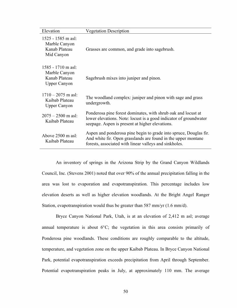
50
Elevation Vegetation Description 1525 - 1585 m asl: Marble Canyon Kanab Plateau Mid Canyon
Grasses are common, and grade into sagebrush.
1585 - 1710 m asl: Marble Canyon Kanab Plateau Upper Canyon
Sagebrush mixes into juniper and pinon.
1710 – 2075 m asl: Kaibab Plateau Upper Canyon
The woodland complex: juniper and pinon with sage and grass undergrowth.
2075 – 2500 m asl: Kaibab Plateau
Ponderosa pine forest dominates, with shrub oak and locust at lower elevations. Note: locust is a good indicator of groundwater seepage. Aspen is present at higher elevations.
Above 2500 m asl: Kaibab Plateau
Aspen and ponderosa pine begin to grade into spruce, Douglas fir. And white fir. Open grasslands are found in the upper montane forests, associated with linear valleys and sinkholes.
An inventory of springs in the Arizona Strip by the Grand Canyon Wildlands
Council, Inc. (Stevens 2001) noted that over 90% of the annual precipitation falling in the
area was lost to evaporation and evapotranspiration. This percentage includes low
elevation deserts as well as higher elevation woodlands. At the Bright Angel Ranger
Station, evapotranspiration would thus be greater than 587 mm/yr (1.6 mm/d).
Bryce Canyon National Park, Utah, is at an elevation of 2,412 m asl; average
annual temperature is about 6°C; the vegetation in this area consists primarily of
Ponderosa pine woodlands. These conditions are roughly comparable to the altitude,
temperature, and vegetation zone on the upper Kaibab Plateau. In Bryce Canyon National
Park, potential evapotranspiration exceeds precipitation from April through September.
Potential evapotranspiration peaks in July, at approximately 110 mm. The average
51
potential evapotranspiration during the summer (April through September) is
approximately 80 mm (~0.44 mm/d). From October through March, precipitation is equal
to or greater than potential evapotranspiration (Spence 1999).
The Rocky Mountain Research Station collects data in the Beaver Creek
watershed (http://ag.arizona.edu.OALS/watershed/beaver/climate.html), which is located
in north-central area of Arizona and is a semi-arid high elevation watershed. Pine
woodlands are found at higher elevations, where the average annual temperature is 7oC.
In this environment, the estimated annual evapotranspiration is 500 mm (1.37 mm/d).
This value was determined by calculating the difference between annual precipitation and
stream flow.
The Arizona Meteorological Network (2005) reports that the cumulative 2003
potential evapotranspiration for Flagstaff (elevation 2056 m asl) was 89 – 99.8 mm (0.24
– 0.27 mm/d).
Evapotranspiration and snow sublimation in ponderosa pine forests at altitudes of
approximately 2100-2700 m asl were reviewed as part of an environmental impact
investigation at Arizona Snowbowl ski resort (U.S. Forest Service 2005). The report cited
data collected in a number of studies that can also be applied to the Kaibab Plateau. Snow
sublimation rates were measured during the winters of 1990 and 1991 (an unusually dry
period) at two sites in Flagstaff, Arizona (elevation ~2100 m asl). Over the course of the
experiment, mean daily evapo-sublimation was 0.152 mm; the maximum amount of 7.87
mm occurred on a clear, dry, windy day. While sublimation on San Francisco Mountain
is expected to be highly variable, 60 - 90% snow pack loss is considered a reasonable
approximation. An average annual evapotranspiration rate from 1993-1996 at ponderosa

52
pine forests in northern New Mexico was 457.2 mm (1.25 mm/d) (US Forest Service
2005).
Transpiration data were collected at Hart Prairie, near Flagstaff, Arizona during
the 129-day growing season in the summer of 2000. This site is slightly below 2,800 m
asl, which makes it a good comparison to the Kaibab Plateau. In Hart Prairie, water use
by the prairie communities was between 1.8 and 5.8 mm per day (Springer et al, in press).
In summary, annual evapotranspiration rates for sites comparable to the Kaibab
Plateau range from 0.24 to 1.6 mm/d. Evapo-sublimation during the winter ranges from
1.52 to 7.87 to mm/d. Evapotranspiration during the summer ranges from 0.44 to 5.8
mm/d. It is expected that the Kaibab Plateau, which at its crest attains elevations slightly
above those mentioned here, has evapotranspiration and sublimation rates on the lower
end of these ranges.
Spring Discharge
Springs have been mapped in geologic units above the R-aquifer in the study area
(Huntoon 1970; U.S Forest Service 1994; Billingsley et al 2000; Stevens 2002b). Spring
locations correlate to geologic contacts, bedding planes, and structural features on the
plateau (Figure 13). In the Supai, Toroweap and Kaibab Formations, springs occur in
sandstone layers above impermeable shale and/or unfractured carbonate and chert. They
are most active during the wet season, but discharge less than a gallon per day (0.01
m3/d) (Huntoon 1970). Some notable exceptions are rare small springs at the contact
between the Supai Group and the Redwall Formation. One of these, along the North
Kaibab Trail in Roaring Springs Canyon, may discharge up to 30 m3/d during the late
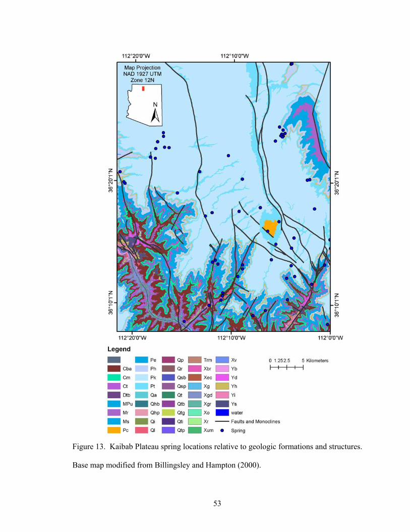
53
Figure 13. Kaibab Plateau spring locations relative to geologic formations and structures.
Base map modified from Billingsley and Hampton (2000).
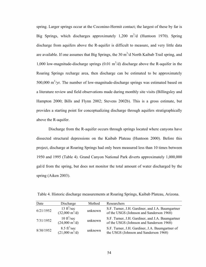
54
spring. Larger springs occur at the Coconino-Hermit contact; the largest of these by far is
Big Springs, which discharges approximately 1,200 m3/d (Huntoon 1970). Spring
discharge from aquifers above the R-aquifer is difficult to measure, and very little data
are available. If one assumes that Big Springs, the 30 m3/d North Kaibab Trail spring, and
1,000 low-magnitude-discharge springs (0.01 m3/d) discharge above the R-aquifer in the
Roaring Springs recharge area, then discharge can be estimated to be approximately
500,000 m3/yr. The number of low-magnitude-discharge springs was estimated based on
a literature review and field observations made during monthly site visits (Billingsley and
Hampton 2000; Bills and Flynn 2002; Stevens 2002b). This is a gross estimate, but
provides a starting point for conceptualizing discharge through aquifers stratigraphically
above the R-aquifer.
Discharge from the R-aquifer occurs through springs located where canyons have
dissected structural depressions on the Kaibab Plateau (Huntoon 2000). Before this
project, discharge at Roaring Springs had only been measured less than 10 times between
1950 and 1995 (Table 4). Grand Canyon National Park diverts approximately 1,000,000
gal/d from the spring, but does not monitor the total amount of water discharged by the
spring (Aiken 2003).
Table 4. Historic discharge measurements at Roaring Springs, Kaibab Plateau, Arizona.
Date Discharge Method Researchers
6/21/1952 13 ft3/sec (32,000 m3/d) unknown S.F. Turner, J.H. Gardiner, and J.A. Baumgartner
of the USGS (Johnson and Sanderson 1968)
7/31/1952 10 ft3/sec (24,000 m3/d) unknown S.F. Turner, J.H. Gardiner, and J.A. Baumgartner
of the USGS (Johnson and Sanderson 1968)
8/30/1952 8.5 ft3/sec (21,000 m3/d) unknown S.F. Turner, J.H. Gardiner, J.A. Baumgartner of
the USGS (Johnson and Sanderson 1968)
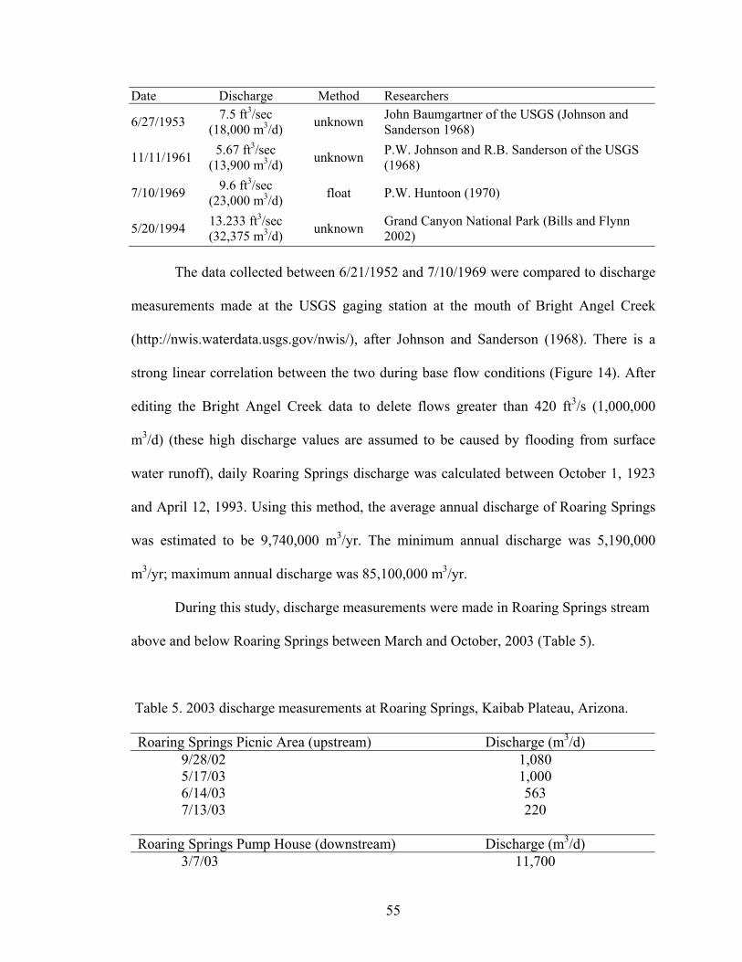
55
Date Discharge Method Researchers
6/27/1953 7.5 ft3/sec (18,000 m3/d) unknown John Baumgartner of the USGS (Johnson and
Sanderson 1968)
11/11/1961 5.67 ft3/sec (13,900 m3/d) unknown P.W. Johnson and R.B. Sanderson of the USGS
(1968)
7/10/1969 9.6 ft3/sec (23,000 m3/d) float P.W. Huntoon (1970)
5/20/1994 13.233 ft3/sec (32,375 m3/d) unknown Grand Canyon National Park (Bills and Flynn
2002)
The data collected between 6/21/1952 and 7/10/1969 were compared to discharge
measurements made at the USGS gaging station at the mouth of Bright Angel Creek
(http://nwis.waterdata.usgs.gov/nwis/), after Johnson and Sanderson (1968). There is a
strong linear correlation between the two during base flow conditions (Figure 14). After
editing the Bright Angel Creek data to delete flows greater than 420 ft3/s (1,000,000
m3/d) (these high discharge values are assumed to be caused by flooding from surface
water runoff), daily Roaring Springs discharge was calculated between October 1, 1923
and April 12, 1993. Using this method, the average annual discharge of Roaring Springs
was estimated to be 9,740,000 m3/yr. The minimum annual discharge was 5,190,000
m3/yr; maximum annual discharge was 85,100,000 m3/yr.
During this study, discharge measurements were made in Roaring Springs stream
above and below Roaring Springs between March and October, 2003 (Table 5).
Table 5. 2003 discharge measurements at Roaring Springs, Kaibab Plateau, Arizona.
Roaring Springs Picnic Area (upstream) Discharge (m3/d) 9/28/02 1,080 5/17/03 1,000 6/14/03 563 7/13/03 220 Roaring Springs Pump House (downstream) Discharge (m3/d) 3/7/03 11,700
56
4/11/03 14,100 5/17/03 51,100 6/14/03 8,700 7/13/03 10,600 9/3/03 8,520 10/11/03 9,010
The discharge data collected upstream of Roaring Springs were used to estimate
diffuse flow through the R-aquifer. The average daily discharge from the aquifer up-
gradient of Roaring Springs was 716 m3/d; average annual discharge was 261,000 m3.
Discharge data collected immediately downstream of the Roaring Springs
complex were compared to water-level data collected by the pressure transducer installed
at this location to build a stage-discharge relationship (Figure 15). High frequency
fluctuation in stream stage is the primary cause for the low R2 value of modeled stage-
discharge relationship. Calculated spring discharge may realistically vary by ±2,000
m3/d.
Because the stream pressure transducer failed between April 12 and May 17,
2003, discharge for this time period was determined by developing a relationship
between stream discharge and turbidity (measured at the Roaring Springs pump house
daily) (Figure 16). This relationship also allows discharge to be calculated for future
seasons. The validity of this method was discussed in Wilkinson (2000). It has also been
substantiated by field observations at Roaring Springs. The primary limitation of this
method is the sporadic turbidity record; data were only collected when NPS staff were
able to visit the pump house (Aiken 2003).
A relationship was also defined between stage in Roaring Springs Stream and in
Roaring Springs Cave for the time period when both pressure transducers were
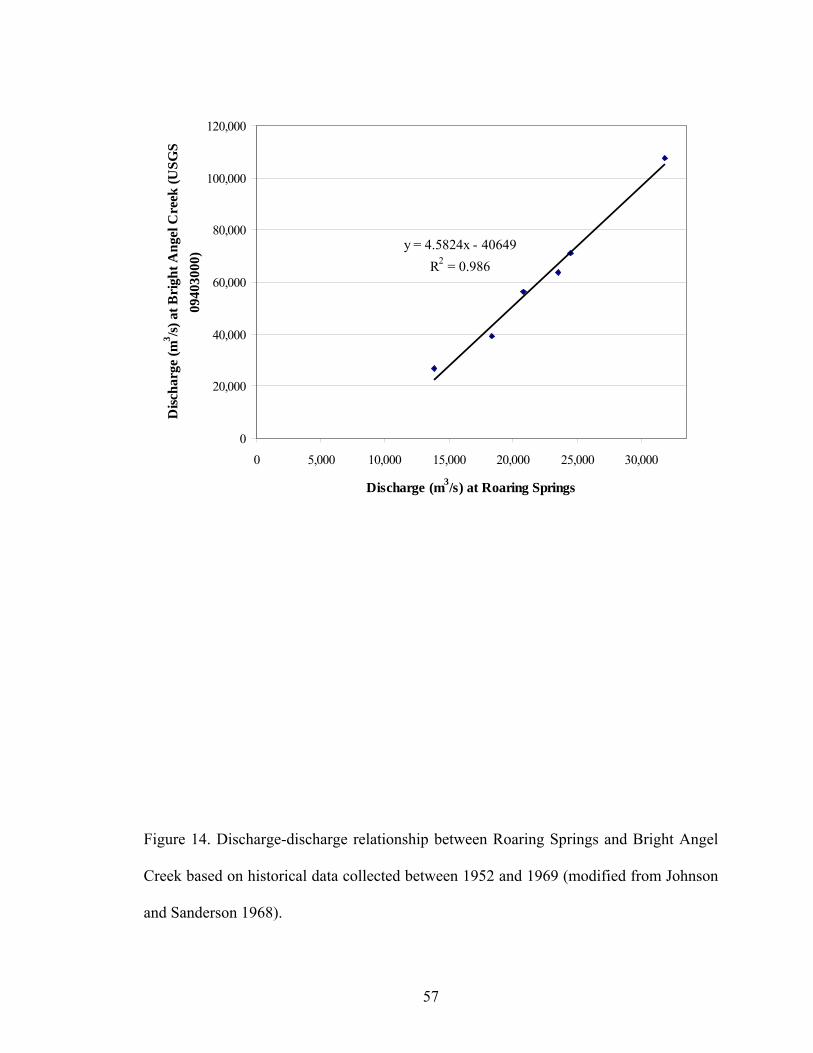
57
Figure 14. Discharge-discharge relationship between Roaring Springs and Bright Angel
Creek based on historical data collected between 1952 and 1969 (modified from Johnson
and Sanderson 1968).
Comparison of discharge in Bright Angel Creek and Roaring Springs, Grand Canyon, Arizona
y = 4.5824x - 40649R2 = 0.986
0
20,000
40,000
60,000
80,000
100,000
120,000
0 5,000 10,000 15,000 20,000 25,000 30,000
Discharge (m3/s) at Roaring Springs
Disc
harg
e (m
3 /s) a
t Bri
ght A
ngel
Cre
ek (U
SGS
0940
3000
)
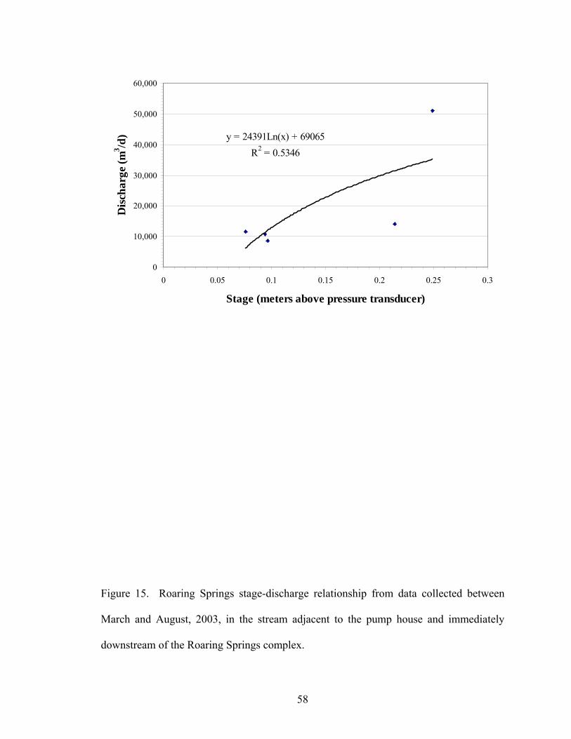
58
y = 24391Ln(x) + 69065R2 = 0.5346
0
10,000
20,000
30,000
40,000
50,000
60,000
0 0.05 0.1 0.15 0.2 0.25 0.3
Stage (meters above pressure transducer)
Dis
char
ge (m
3 /d)
Figure 15. Roaring Springs stage-discharge relationship from data collected between
March and August, 2003, in the stream adjacent to the pump house and immediately
downstream of the Roaring Springs complex.
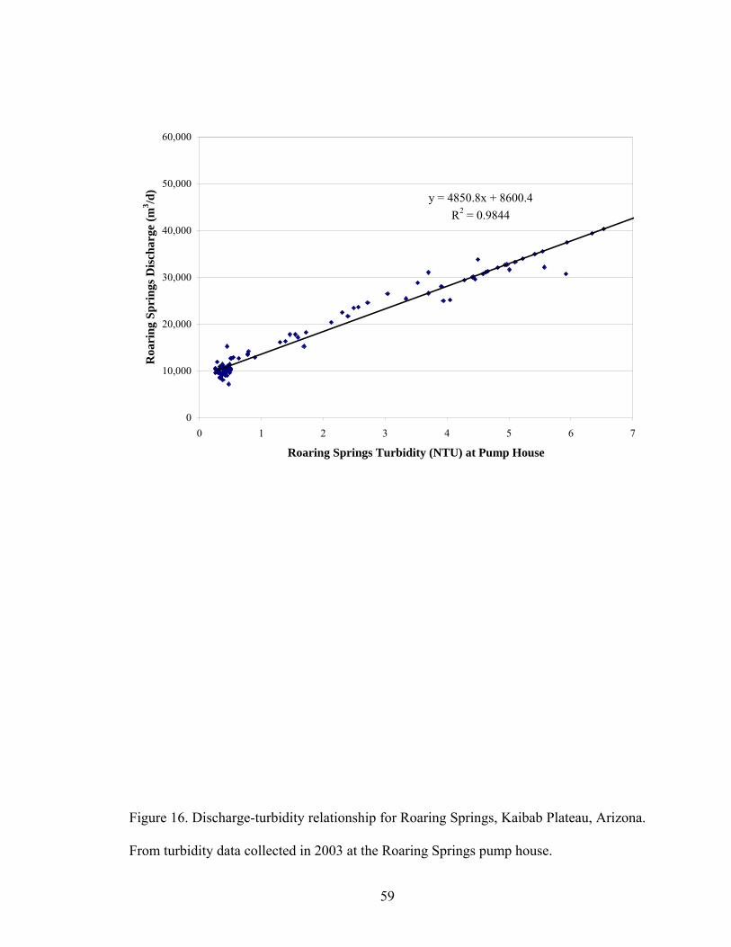
59
y = 4850.8x + 8600.4R2 = 0.9844
0
10,000
20,000
30,000
40,000
50,000
60,000
0 1 2 3 4 5 6 7
Roaring Springs Turbidity (NTU) at Pump House
Roa
ring
Spr
ings
Dis
char
ge (m
3 /d)
Figure 16. Discharge-turbidity relationship for Roaring Springs, Kaibab Plateau, Arizona.
From turbidity data collected in 2003 at the Roaring Springs pump house.
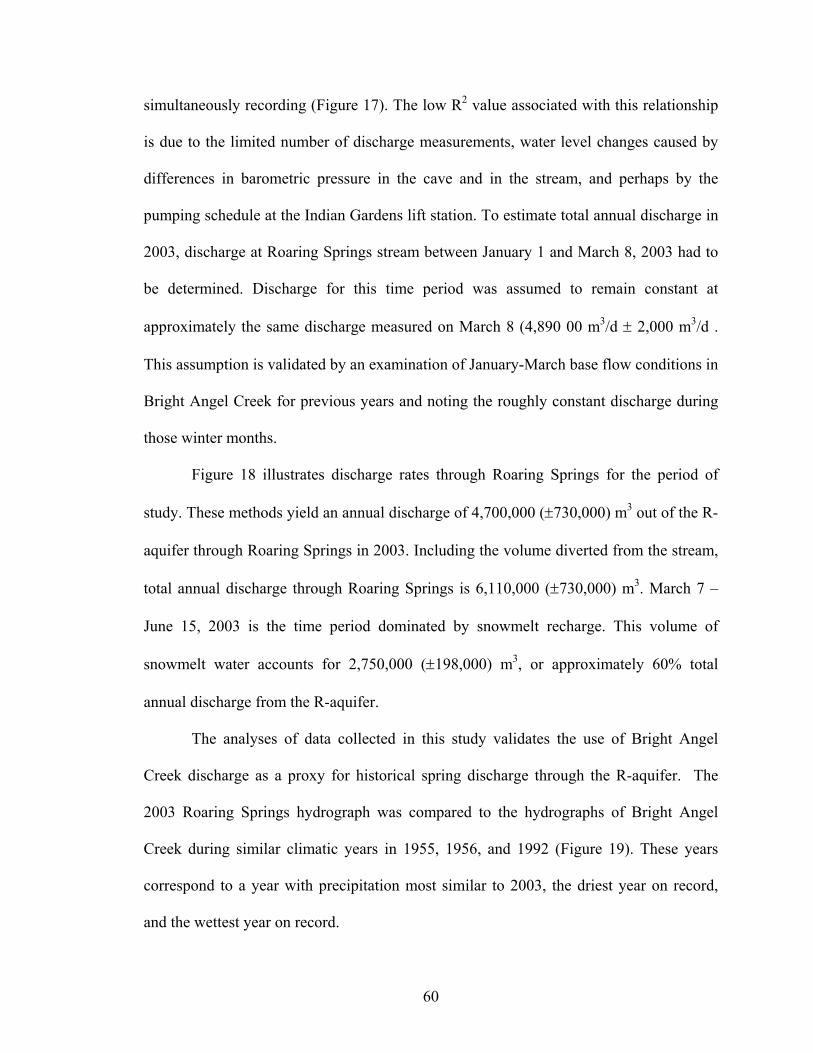
60
simultaneously recording (Figure 17). The low R2 value associated with this relationship
is due to the limited number of discharge measurements, water level changes caused by
differences in barometric pressure in the cave and in the stream, and perhaps by the
pumping schedule at the Indian Gardens lift station. To estimate total annual discharge in
2003, discharge at Roaring Springs stream between January 1 and March 8, 2003 had to
be determined. Discharge for this time period was assumed to remain constant at
approximately the same discharge measured on March 8 (4,890 00 m3/d ± 2,000 m3/d .
This assumption is validated by an examination of January-March base flow conditions in
Bright Angel Creek for previous years and noting the roughly constant discharge during
those winter months.
Figure 18 illustrates discharge rates through Roaring Springs for the period of
study. These methods yield an annual discharge of 4,700,000 (±730,000) m3 out of the R-
aquifer through Roaring Springs in 2003. Including the volume diverted from the stream,
total annual discharge through Roaring Springs is 6,110,000 (±730,000) m3. March 7 –
June 15, 2003 is the time period dominated by snowmelt recharge. This volume of
snowmelt water accounts for 2,750,000 (±198,000) m3, or approximately 60% total
annual discharge from the R-aquifer.
The analyses of data collected in this study validates the use of Bright Angel
Creek discharge as a proxy for historical spring discharge through the R-aquifer. The
2003 Roaring Springs hydrograph was compared to the hydrographs of Bright Angel
Creek during similar climatic years in 1955, 1956, and 1992 (Figure 19). These years
correspond to a year with precipitation most similar to 2003, the driest year on record,
and the wettest year on record.
61
Figure 17. Stage-discharge relationship between Roaring Springs Stream and Roaring
Springs Cave, Kaibab Plateau, Arizona, based on daily data collected between July 13
and August 15, 2003.
Stage-Discharge Relationship between Roaring Springs Cave Pressure Transducer and Roaring Springs Stream
Calculated Discharge
y = 13705x + 3417.6R2 = 0.3536
8,000
8,500
9,000
9,500
10,000
10,500
11,000
11,500
12,000
12,500
0.4 0.42 0.44 0.46 0.48 0.5 0.52 0.54 0.56
Roaring Springs Cave Pressure Transducer Stage(m above pressure transducer)
Roa
ring
Spr
ings
Str
eam
Disc
harg
e (m
3 /d)
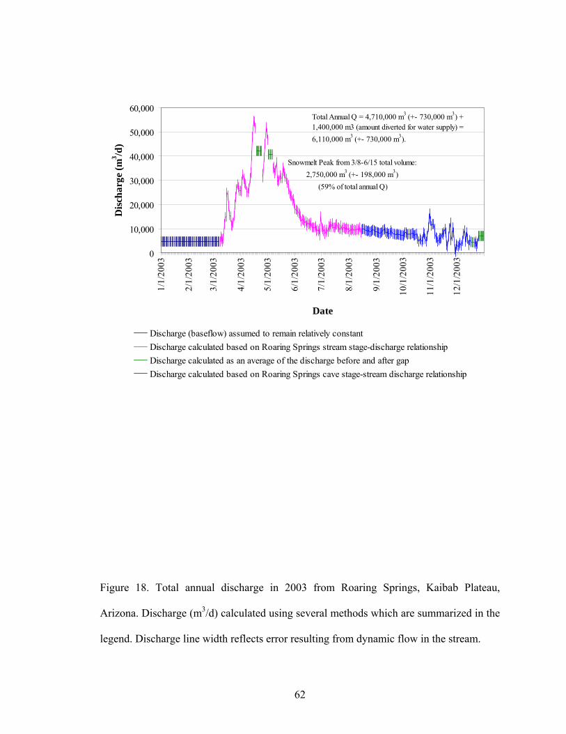
62
0
10,000
20,000
30,000
40,000
50,000
60,000
1/1/
2003
2/1/
2003
3/1/
2003
4/1/
2003
5/1/
2003
6/1/
2003
7/1/
2003
8/1/
2003
9/1/
2003
10/1
/200
3
11/1
/200
3
12/1
/200
3
Date
Dis
char
ge (m
3 /d)
Discharge (baseflow) assumed to remain relatively constantDischarge calculated based on Roaring Springs stream stage-discharge relationshipDischarge calculated as an average of the discharge before and after gapDischarge calculated based on Roaring Springs cave stage-stream discharge relationship
Total Annual Q = 4,710,000 m3 (+- 730,000 m3) + 1,400,000 m3 (amount diverted for water supply) = 6,110,000 m3 (+- 730,000 m3).
Snowmelt Peak from 3/8-6/15 total volume: 2,750,000 m3 (+- 198,000 m3)
(59% of total annual Q)
Figure 18. Total annual discharge in 2003 from Roaring Springs, Kaibab Plateau,
Arizona. Discharge (m3/d) calculated using several methods which are summarized in the
legend. Discharge line width reflects error resulting from dynamic flow in the stream.
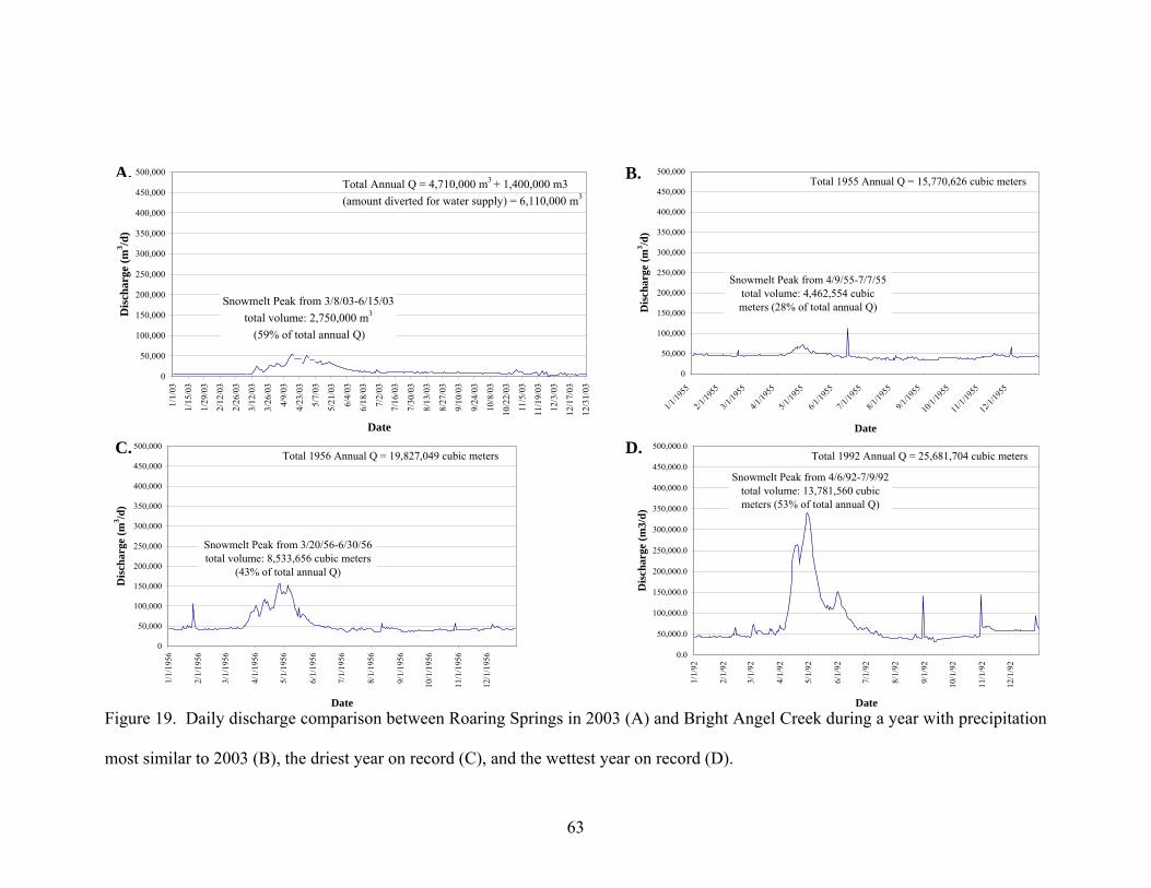
63
0
50,000
100,000
150,000
200,000
250,000
300,000
350,000
400,000
450,000
500,0001/
1/03
1/15
/03
1/29
/03
2/12
/03
2/26
/03
3/12
/03
3/26
/03
4/9/
03
4/23
/03
5/7/
03
5/21
/03
6/4/
03
6/18
/03
7/2/
03
7/16
/03
7/30
/03
8/13
/03
8/27
/03
9/10
/03
9/24
/03
10/8
/03
10/2
2/03
11/5
/03
11/1
9/03
12/3
/03
12/1
7/03
12/3
1/03
Date
Dis
char
ge (m
3 /d)
Total Annual Q = 4,710,000 m3 + 1,400,000 m3 (amount diverted for water supply) = 6,110,000 m3
Snowmelt Peak from 3/8/03-6/15/03 total volume: 2,750,000 m3
(59% of total annual Q)
0
50,000
100,000
150,000
200,000
250,000
300,000
350,000
400,000
450,000
500,000
1/1/19
552/1
/1955
3/1/19
554/1
/1955
5/1/19
556/1
/1955
7/1/19
558/1
/1955
9/1/19
5510
/1/19
5511
/1/19
5512
/1/19
55
Date
Dis
char
ge (m
3 /d)
Snowmelt Peak from 4/9/55-7/7/55 total volume: 4,462,554 cubic meters (28% of total annual Q)
Total 1955 Annual Q = 15,770,626 cubic meters
0.0
50,000.0
100,000.0
150,000.0
200,000.0
250,000.0
300,000.0
350,000.0
400,000.0
450,000.0
500,000.0
1/1/
92
2/1/
92
3/1/
92
4/1/
92
5/1/
92
6/1/
92
7/1/
92
8/1/
92
9/1/
92
10/1
/92
11/1
/92
12/1
/92
Date
Dis
char
ge (m
3/d)
Snowmelt Peak from 4/6/92-7/9/92 total volume: 13,781,560 cubic meters (53% of total annual Q)
Total 1992 Annual Q = 25,681,704 cubic meters
0
50,000
100,000
150,000
200,000
250,000
300,000
350,000
400,000
450,000
500,000
1/1/
1956
2/1/
1956
3/1/
1956
4/1/
1956
5/1/
1956
6/1/
1956
7/1/
1956
8/1/
1956
9/1/
1956
10/1
/195
6
11/1
/195
6
12/1
/195
6
Date
Dis
char
ge (m
3 /d)
Snowmelt Peak from 3/20/56-6/30/56 total volume: 8,533,656 cubic meters
(43% of total annual Q)
Total 1956 Annual Q = 19,827,049 cubic meters
Figure 19. Daily discharge comparison between Roaring Springs in 2003 (A) and Bright Angel Creek during a year with precipitation
most similar to 2003 (B), the driest year on record (C), and the wettest year on record (D).
A. B.
C. D.
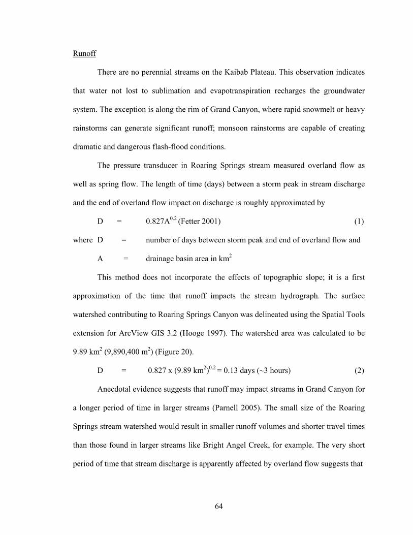
64
Runoff
There are no perennial streams on the Kaibab Plateau. This observation indicates
that water not lost to sublimation and evapotranspiration recharges the groundwater
system. The exception is along the rim of Grand Canyon, where rapid snowmelt or heavy
rainstorms can generate significant runoff; monsoon rainstorms are capable of creating
dramatic and dangerous flash-flood conditions.
The pressure transducer in Roaring Springs stream measured overland flow as
well as spring flow. The length of time (days) between a storm peak in stream discharge
and the end of overland flow impact on discharge is roughly approximated by
D = 0.827A0.2 (Fetter 2001) (1)
where D = number of days between storm peak and end of overland flow and
A = drainage basin area in km2
This method does not incorporate the effects of topographic slope; it is a first
approximation of the time that runoff impacts the stream hydrograph. The surface
watershed contributing to Roaring Springs Canyon was delineated using the Spatial Tools
extension for ArcView GIS 3.2 (Hooge 1997). The watershed area was calculated to be
9.89 km2 (9,890,400 m2) (Figure 20).
D = 0.827 x (9.89 km2)0.2 = 0.13 days (~3 hours) (2)
Anecdotal evidence suggests that runoff may impact streams in Grand Canyon for
a longer period of time in larger streams (Parnell 2005). The small size of the Roaring
Springs stream watershed would result in smaller runoff volumes and shorter travel times
than those found in larger streams like Bright Angel Creek, for example. The very short
period of time that stream discharge is apparently affected by overland flow suggests that
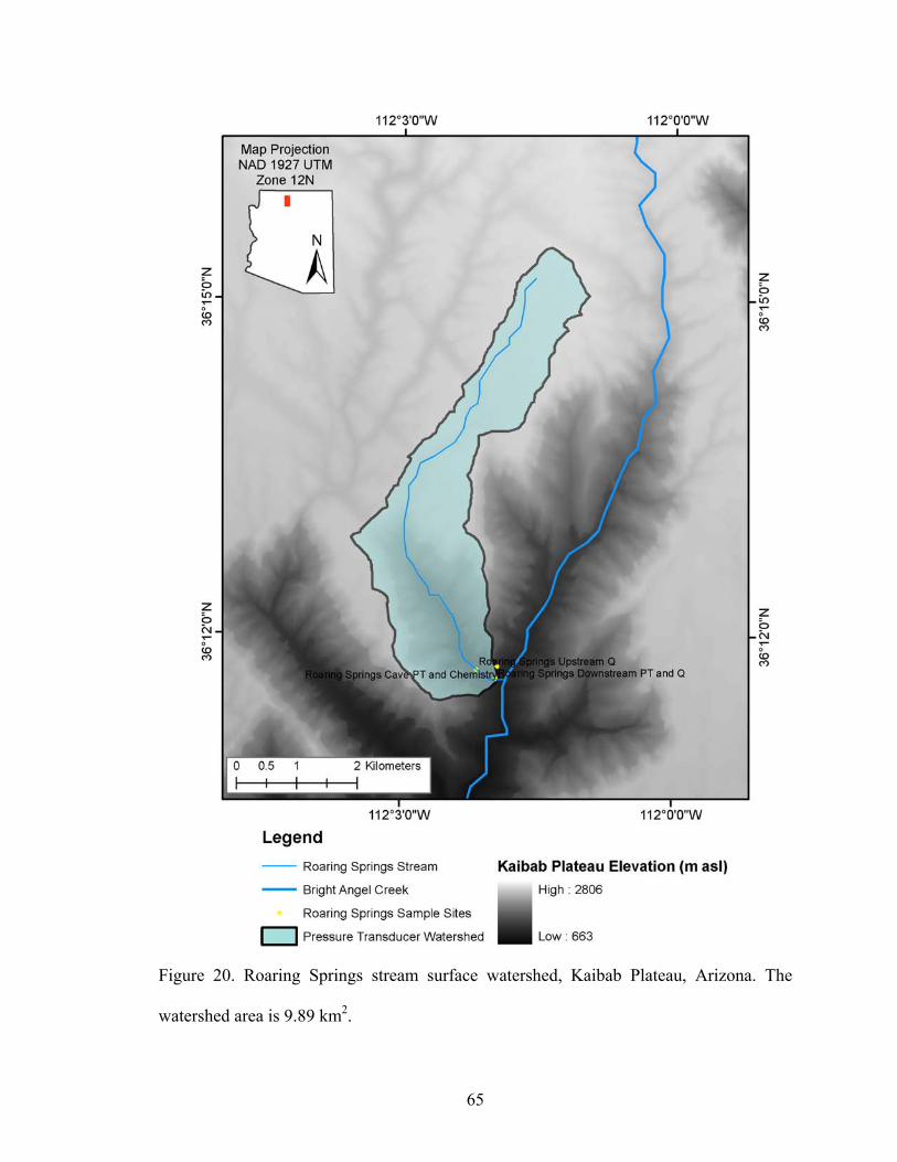
65
Figure 20. Roaring Springs stream surface watershed, Kaibab Plateau, Arizona. The
watershed area is 9.89 km2.
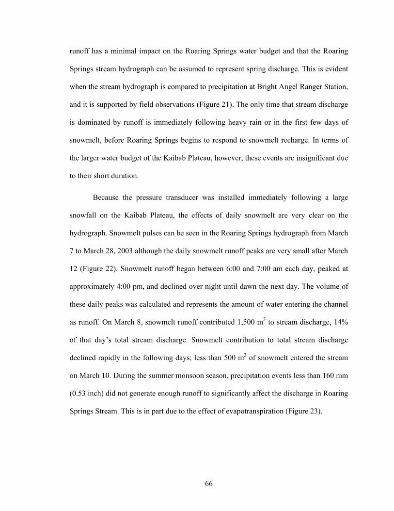
66
runoff has a minimal impact on the Roaring Springs water budget and that the Roaring
Springs stream hydrograph can be assumed to represent spring discharge. This is evident
when the stream hydrograph is compared to precipitation at Bright Angel Ranger Station,
and it is supported by field observations (Figure 21). The only time that stream discharge
is dominated by runoff is immediately following heavy rain or in the first few days of
snowmelt, before Roaring Springs begins to respond to snowmelt recharge. In terms of
the larger water budget of the Kaibab Plateau, however, these events are insignificant due
to their short duration.
Because the pressure transducer was installed immediately following a large
snowfall on the Kaibab Plateau, the effects of daily snowmelt are very clear on the
hydrograph. Snowmelt pulses can be seen in the Roaring Springs hydrograph from March
7 to March 28, 2003 although the daily snowmelt runoff peaks are very small after March
12 (Figure 22). Snowmelt runoff began between 6:00 and 7:00 am each day, peaked at
approximately 4:00 pm, and declined over night until dawn the next day. The volume of
these daily peaks was calculated and represents the amount of water entering the channel
as runoff. On March 8, snowmelt runoff contributed 1,500 m3 to stream discharge, 14%
of that day’s total stream discharge. Snowmelt contribution to total stream discharge
declined rapidly in the following days; less than 500 m3 of snowmelt entered the stream
on March 10. During the summer monsoon season, precipitation events less than 160 mm
(0.53 inch) did not generate enough runoff to significantly affect the discharge in Roaring
Springs Stream. This is in part due to the effect of evapotranspiration (Figure 23).
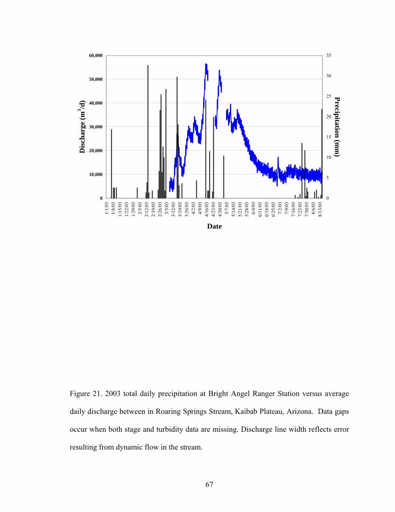
67
0
10,000
20,000
30,000
40,000
50,000
60,000
1/1/
031/
8/03
1/15
/03
1/22
/03
1/29
/03
2/5/
032/
12/0
32/
19/0
32/
26/0
33/
5/03
3/12
/03
3/19
/03
3/26
/03
4/2/
034/
9/03
4/16
/03
4/23
/03
4/30
/03
5/7/
035/
14/0
35/
21/0
35/
28/0
36/
4/03
6/11
/03
6/18
/03
6/25
/03
7/2/
037/
9/03
7/16
/03
7/23
/03
7/30
/03
8/6/
038/
13/0
3
Date
Dis
char
ge (m
3 /d)
0
5
10
15
20
25
30
35Precipitation (m
m)
Figure 21. 2003 total daily precipitation at Bright Angel Ranger Station versus average
daily discharge between in Roaring Springs Stream, Kaibab Plateau, Arizona. Data gaps
occur when both stage and turbidity data are missing. Discharge line width reflects error
resulting from dynamic flow in the stream.
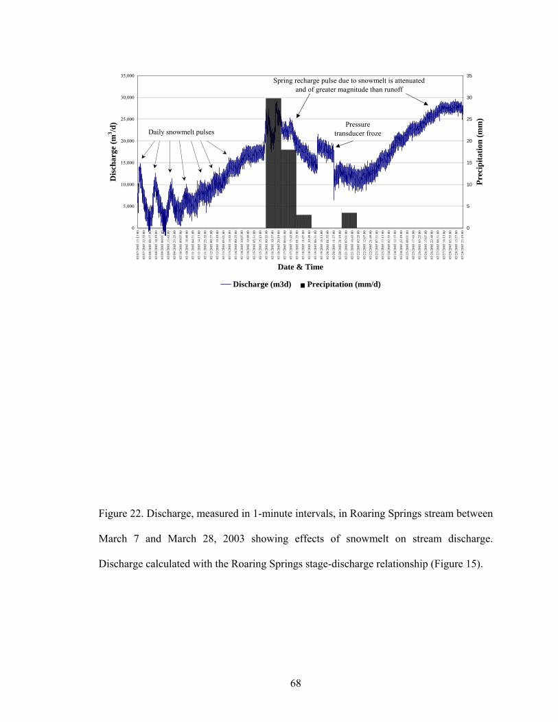
68
0
5,000
10,000
15,000
20,000
25,000
30,000
35,000
03/0
7/20
03 1
3:13
:00
03/0
7/20
03 2
2:55
:00
03/0
8/20
03 0
8:37
:00
03/0
8/20
03 1
8:19
:00
03/0
9/20
03 0
4:01
:00
03/0
9/20
03 1
3:43
:00
03/0
9/20
03 2
3:25
:00
03/1
0/20
03 0
9:07
:00
03/1
0/20
03 1
8:49
:00
03/1
1/20
03 0
4:31
:00
03/1
1/20
03 1
4:13
:00
03/1
1/20
03 2
3:55
:00
03/1
2/20
03 0
9:37
:00
03/1
2/20
03 1
9:19
:00
03/1
3/20
03 0
5:01
:00
03/1
3/20
03 1
4:43
:00
03/1
4/20
03 0
0:25
:00
03/1
4/20
03 1
0:07
:00
03/1
4/20
03 1
9:49
:00
03/1
5/20
03 0
5:31
:00
03/1
5/20
03 1
5:13
:00
03/1
6/20
03 0
0:55
:00
03/1
6/20
03 1
0:37
:00
03/1
6/20
03 2
0:19
:00
03/1
7/20
03 0
6:01
:00
03/1
7/20
03 1
5:43
:00
03/1
8/20
03 0
1:25
:00
03/1
8/20
03 1
1:07
:00
03/1
8/20
03 2
0:49
:00
03/1
9/20
03 0
6:31
:00
03/1
9/20
03 1
6:13
:00
03/2
0/20
03 0
1:55
:00
03/2
0/20
03 1
1:37
:00
03/2
0/20
03 2
1:19
:00
03/2
1/20
03 0
7:01
:00
03/2
1/20
03 1
6:43
:00
03/2
2/20
03 0
2:25
:00
03/2
2/20
03 1
2:07
:00
03/2
2/20
03 2
1:49
:00
03/2
3/20
03 0
7:31
:00
03/2
3/20
03 1
7:13
:00
03/2
4/20
03 0
2:55
:00
03/2
4/20
03 1
2:37
:00
03/2
4/20
03 2
2:19
:00
03/2
5/20
03 0
8:01
:00
03/2
5/20
03 1
7:43
:00
03/2
6/20
03 0
3:25
:00
03/2
6/20
03 1
3:07
:00
03/2
6/20
03 2
2:49
:00
03/2
7/20
03 0
8:31
:00
03/2
7/20
03 1
8:13
:00
03/2
8/20
03 0
3:55
:00
03/2
8/20
03 1
3:37
:00
03/2
8/20
03 2
3:19
:00
Date & Time
Dis
char
ge (m
3 /d)
0
5
10
15
20
25
30
35
Prec
ipita
tion
(mm
)
Discharge (m3d) Precipitation (mm/d)
Pressure transducer frozeDaily snowmelt pulses
Spring recharge pulse due to snowmelt is attenuated and of greater magnitude than runoff
Figure 22. Discharge, measured in 1-minute intervals, in Roaring Springs stream between
March 7 and March 28, 2003 showing effects of snowmelt on stream discharge.
Discharge calculated with the Roaring Springs stage-discharge relationship (Figure 15).
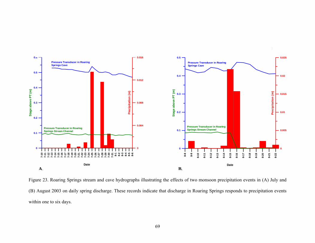
69
Figure 23. Roaring Springs stream and cave hydrographs illustrating the effects of two monsoon precipitation events in (A) July and
(B) August 2003 on daily spring discharge. These records indicate that discharge in Roaring Springs responds to precipitation events
within one to six days.
A. B.
7-10
7-11
7-12
7-13
7-14
7-15
7-16
7-17
7-18
7-19
7-20
7-21
7-22
7-23
7-24
7-25
7-26
7-27
7-28
7-29
7-30
7-31 8-1
8-2
8-3
8-4
8-5
8-6
Date
0
0.1
0.2
0.3
0.4
0.5
0.6
Stag
e ab
ove
PT (m
)
0
0.004
0.008
0.012
0.016
Prec
ipita
tion
(m)
Pressure Transducer in RoaringSprings Cave
Pressure Transducer in RoaringSprings Stream Channel
Reponse in Pressure Transducer Data to Precipitation Event:July 25, 2003
8-8
8-9
8-10
8-11
8-12
8-13
8-14
8-15
8-16
8-17
8-18
8-19
8-20
8-21
8-22
Date
0
0.1
0.2
0.3
0.4
0.5
Stag
e ab
ove
PT (m
)
0
0.005
0.01
0.015
0.02
0.025
Prec
ipita
tion
(m)
Pressure Transducer in RoaringSprings Cave
Pressure Transducer in RoaringSprings Stream Channel
Response in Pressure Transducer Data to Precipitation Event:August 15, 2003
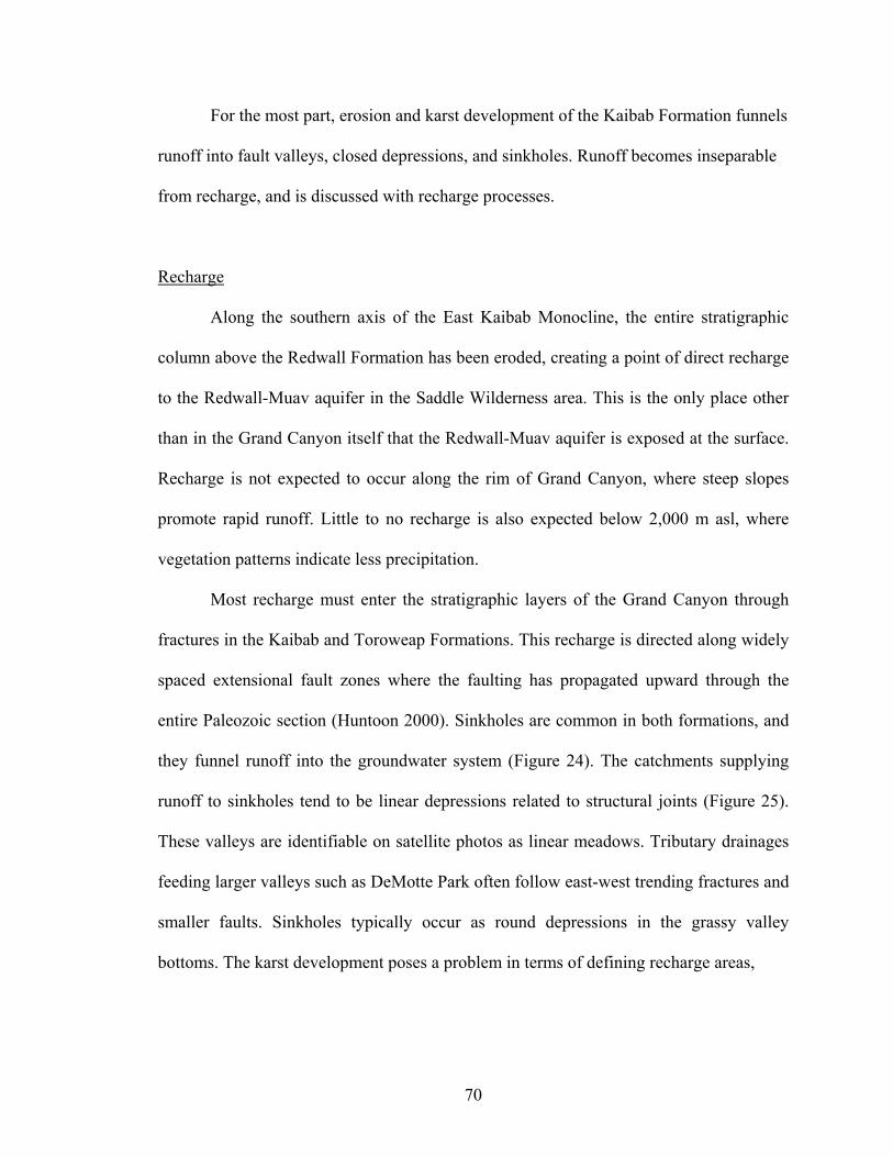
70
For the most part, erosion and karst development of the Kaibab Formation funnels
runoff into fault valleys, closed depressions, and sinkholes. Runoff becomes inseparable
from recharge, and is discussed with recharge processes.
Recharge
Along the southern axis of the East Kaibab Monocline, the entire stratigraphic
column above the Redwall Formation has been eroded, creating a point of direct recharge
to the Redwall-Muav aquifer in the Saddle Wilderness area. This is the only place other
than in the Grand Canyon itself that the Redwall-Muav aquifer is exposed at the surface.
Recharge is not expected to occur along the rim of Grand Canyon, where steep slopes
promote rapid runoff. Little to no recharge is also expected below 2,000 m asl, where
vegetation patterns indicate less precipitation.
Most recharge must enter the stratigraphic layers of the Grand Canyon through
fractures in the Kaibab and Toroweap Formations. This recharge is directed along widely
spaced extensional fault zones where the faulting has propagated upward through the
entire Paleozoic section (Huntoon 2000). Sinkholes are common in both formations, and
they funnel runoff into the groundwater system (Figure 24). The catchments supplying
runoff to sinkholes tend to be linear depressions related to structural joints (Figure 25).
These valleys are identifiable on satellite photos as linear meadows. Tributary drainages
feeding larger valleys such as DeMotte Park often follow east-west trending fractures and
smaller faults. Sinkholes typically occur as round depressions in the grassy valley
bottoms. The karst development poses a problem in terms of defining recharge areas,
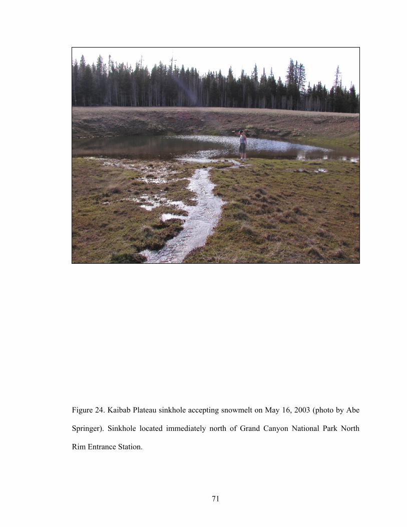
71
Figure 24. Kaibab Plateau sinkhole accepting snowmelt on May 16, 2003 (photo by Abe
Springer). Sinkhole located immediately north of Grand Canyon National Park North
Rim Entrance Station.
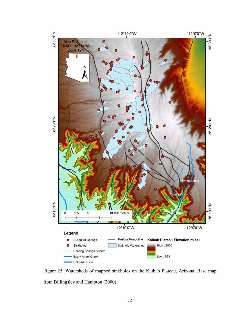
72
Figure 25. Watersheds of mapped sinkholes on the Kaibab Plateau, Arizona. Base map
from Billingsley and Hampton (2000).
Fault or Monocline
73
because water from isolated basins outside of the Roaring Springs stream watershed may
be contributing to spring discharge.
A dynamic average steady-state groundwater flow system is one where discharge
and recharge are in long-term equilibrium (Anderson and Woessner 1992). Recharge to
the Roaring Springs groundwater flow system should therefore be approximately
9,740,000 m3/yr, which is the average annual discharge of Roaring Springs based on a
relationship developed between spring discharge and the 87-year discharge record of
Bright Angel Creek.
Annual recharge across the study area can also be estimated by subtracting annual
evapotranspiration from annual precipitation across the study area. Using this method and
the data presented previously, recharge across the Kaibab Plateau should range from zero
to 290 mm annually, with less recharge occurring at lower, drier elevations.
Recharge is seasonally variable. Most precipitation falls during the winter, when
low temperatures and plant use allow more water to recharge the aquifer system. There is
less precipitation during the summer when evapotranspiration rates are much higher. This
seasonal recharge pattern is apparent on the Roaring Springs hydrograph as a peak during
late spring and declining base flow through the summer monsoon season (Figure 26).
The hydrograph also indicates that recharge is occurring through two different
processes. A large volume of water flows rapidly through the aquifer’s conduit system,
while perennial base flow at the spring is sustained by water discharging from aquifer
storage. The volume of water discharging from Roaring Springs between March 8 and
June 15, 2003 is approximately 2,750,000 m3 (~60% of annual spring discharge). This
large peak in spring discharge corresponds to the snow pack melting on the Kaibab
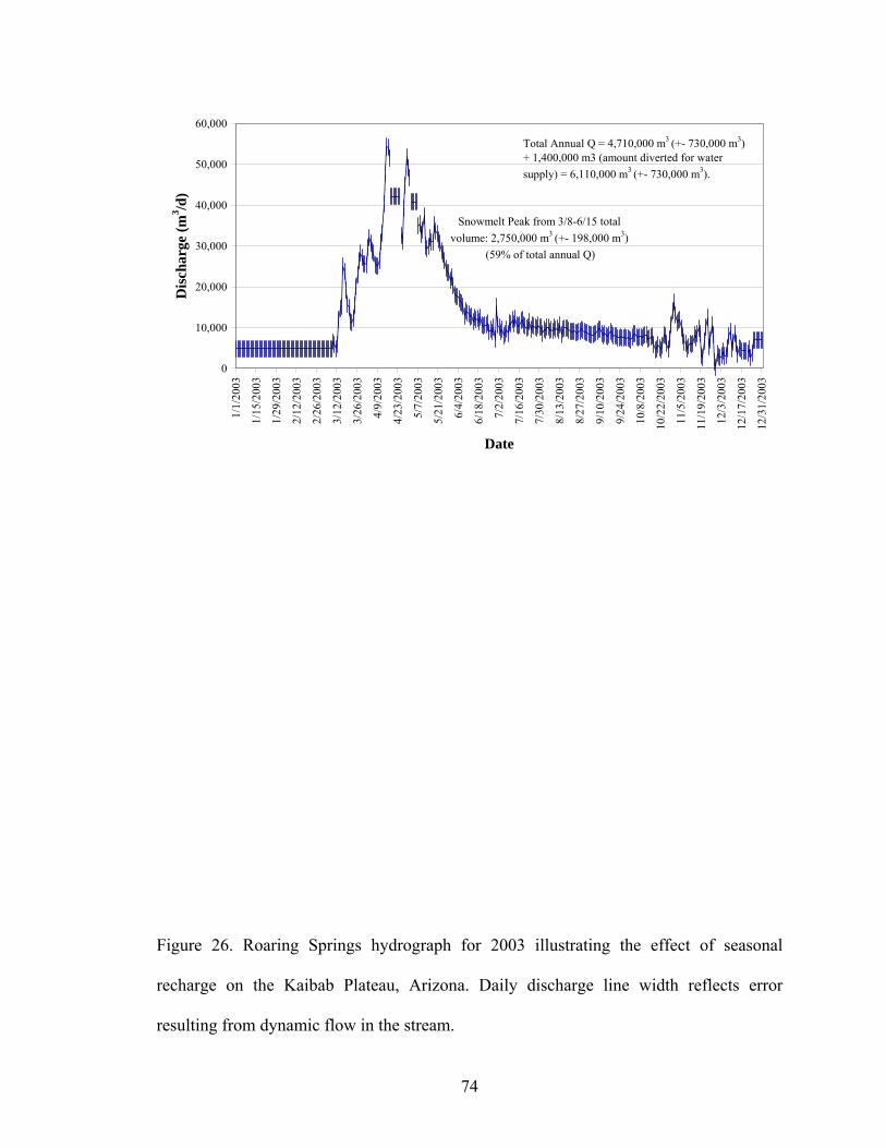
74
0
10,000
20,000
30,000
40,000
50,000
60,000
1/1/
2003
1/15
/200
3
1/29
/200
3
2/12
/200
3
2/26
/200
3
3/12
/200
3
3/26
/200
3
4/9/
2003
4/23
/200
3
5/7/
2003
5/21
/200
3
6/4/
2003
6/18
/200
3
7/2/
2003
7/16
/200
3
7/30
/200
3
8/13
/200
3
8/27
/200
3
9/10
/200
3
9/24
/200
3
10/8
/200
3
10/2
2/20
03
11/5
/200
3
11/1
9/20
03
12/3
/200
3
12/1
7/20
03
12/3
1/20
03
Date
Dis
char
ge (m
3 /d)
Total Annual Q = 4,710,000 m3 (+- 730,000 m3) + 1,400,000 m3 (amount diverted for water supply) = 6,110,000 m3 (+- 730,000 m3).
Snowmelt Peak from 3/8-6/15 total volume: 2,750,000 m3 (+- 198,000 m3)
(59% of total annual Q)
Figure 26. Roaring Springs hydrograph for 2003 illustrating the effect of seasonal
recharge on the Kaibab Plateau, Arizona. Daily discharge line width reflects error
resulting from dynamic flow in the stream.
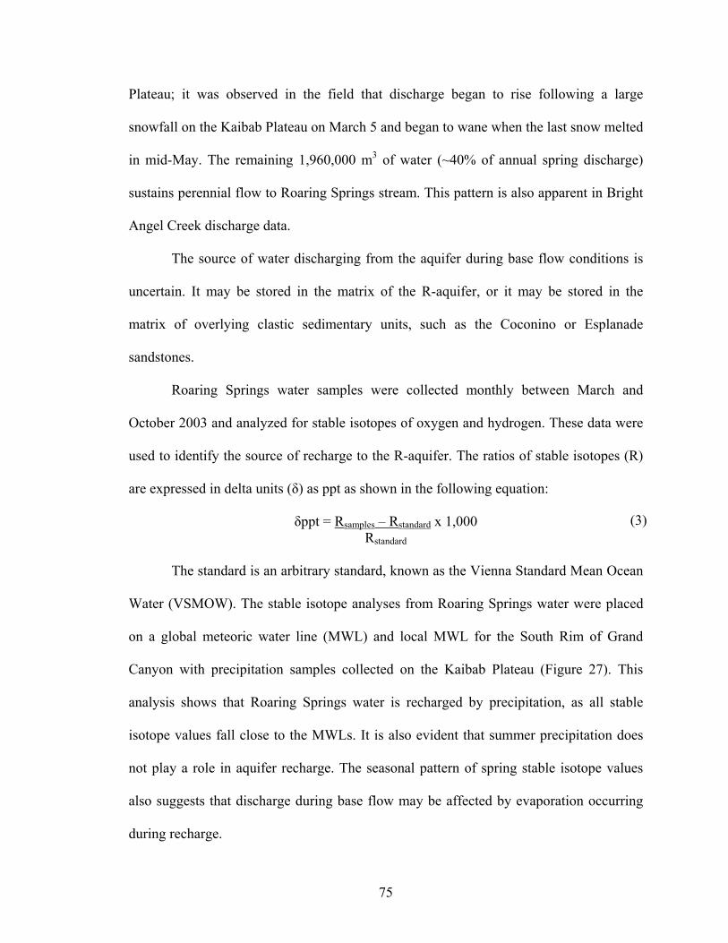
75
Plateau; it was observed in the field that discharge began to rise following a large
snowfall on the Kaibab Plateau on March 5 and began to wane when the last snow melted
in mid-May. The remaining 1,960,000 m3 of water (~40% of annual spring discharge)
sustains perennial flow to Roaring Springs stream. This pattern is also apparent in Bright
Angel Creek discharge data.
The source of water discharging from the aquifer during base flow conditions is
uncertain. It may be stored in the matrix of the R-aquifer, or it may be stored in the
matrix of overlying clastic sedimentary units, such as the Coconino or Esplanade
sandstones.
Roaring Springs water samples were collected monthly between March and
October 2003 and analyzed for stable isotopes of oxygen and hydrogen. These data were
used to identify the source of recharge to the R-aquifer. The ratios of stable isotopes (R)
are expressed in delta units (δ) as ppt as shown in the following equation:
δppt = Rsamples – Rstandard x 1,000 Rstandard
The standard is an arbitrary standard, known as the Vienna Standard Mean Ocean
Water (VSMOW). The stable isotope analyses from Roaring Springs water were placed
on a global meteoric water line (MWL) and local MWL for the South Rim of Grand
Canyon with precipitation samples collected on the Kaibab Plateau (Figure 27). This
analysis shows that Roaring Springs water is recharged by precipitation, as all stable
isotope values fall close to the MWLs. It is also evident that summer precipitation does
not play a role in aquifer recharge. The seasonal pattern of spring stable isotope values
also suggests that discharge during base flow may be affected by evaporation occurring
during recharge.
(3)
76
-120
-110
-100
-90
-80
-70
-60
-50
-40
-30
-20
-15 -14 -13 -12 -11 -10 -9 -8 -7 -6 -5
delta18O (%o)
delta
2 H(%
o)Global MeteoricWater Line (Rozanskiet al 1993)
Kaibab PlateauPrecipitation (Miller2004)
Roaring Springs(Zukosky 1993, Ross2003, Miller 2004)
South Rim MeteoricWater Line (Monroe etal 2004)
Winter Precipitation
SummerPrecipitation
-100
-95
-90
-85
-80
-14 -13.5 -13 -12.5 -12
delta18O (%o)
delta
2 H(%
o)
Global Meteoric Water Line(Rozanski et al 1993)
South Rim Meteoric WaterLine (Monroe et al 2004)
Kaibab Plateau Precipitation(Miller 2004)
Roaring Springs Pre-Snowmelt (Zukosky 1993,Ross 2003)Roaring Springs Snowmelt(Ross 2003)
Roaring Springs Monsoon(Ross 2003)
Roaring Springs Baseflow(Zukosky 1993, Ross 2003,Miller 2004)
Winter Precipitation
Figure 27. Oxygen and hydrogen stable isotope analyses of 1993 and 2003-2004 Roaring
Springs discharge and Kaibab Plateau precipitation.
77
Change in Aquifer Storage
Quinlan and others (1992) recognized that long-term storage in a karst aquifer is
controlled by the distribution of dissolution porosity in relation to the regional base level.
If most porosity in the aquifer is above base level, as is the case with the Kaibab Plateau,
then flow through the aquifer will be rapid and storage minimal. Huntoon (2000) used
similar reasoning to conclude that there is minimal groundwater storage in the unconfined
portions of the R-aquifer, as cave passages tend to be widely spaced and are partially
drained. The distribution of aquifer storage is necessary for transient modeling. This
parameter is not known with any certainty on the Kaibab Plateau. The range of
acceptable values was based on a literature review of similar aquifers (Johnson 2000;
Kessler 2002; Smith and Hunt 2004). Storage values ranged from 0.01-0.50, based on
karst aquifer research in Arizona, Texas and New Mexico.
Flow System
The hydraulic character of karst aquifers is defined by the spatial and temporal
distribution of flow regimes that range from turbulent flow in freely draining conduits to
diffuse laminar flow through narrow fractures, partings, and intergranular pores. Solution
conduits develop along the routes of greatest unsaturated zone water movement, which
are often vertical or steeply dipping fractures. When the steepest pathways are unable to
transmit all the water entering from karst recharge features, water will overflow along the
next steepest pathway such as bedding-plane partings. Turbulent conduits are surrounded
by bedrock that contains only diffuse laminar flow; the diffuse bedrock seepage drains
into these conduits (Ginsberg and Palmer 2002).
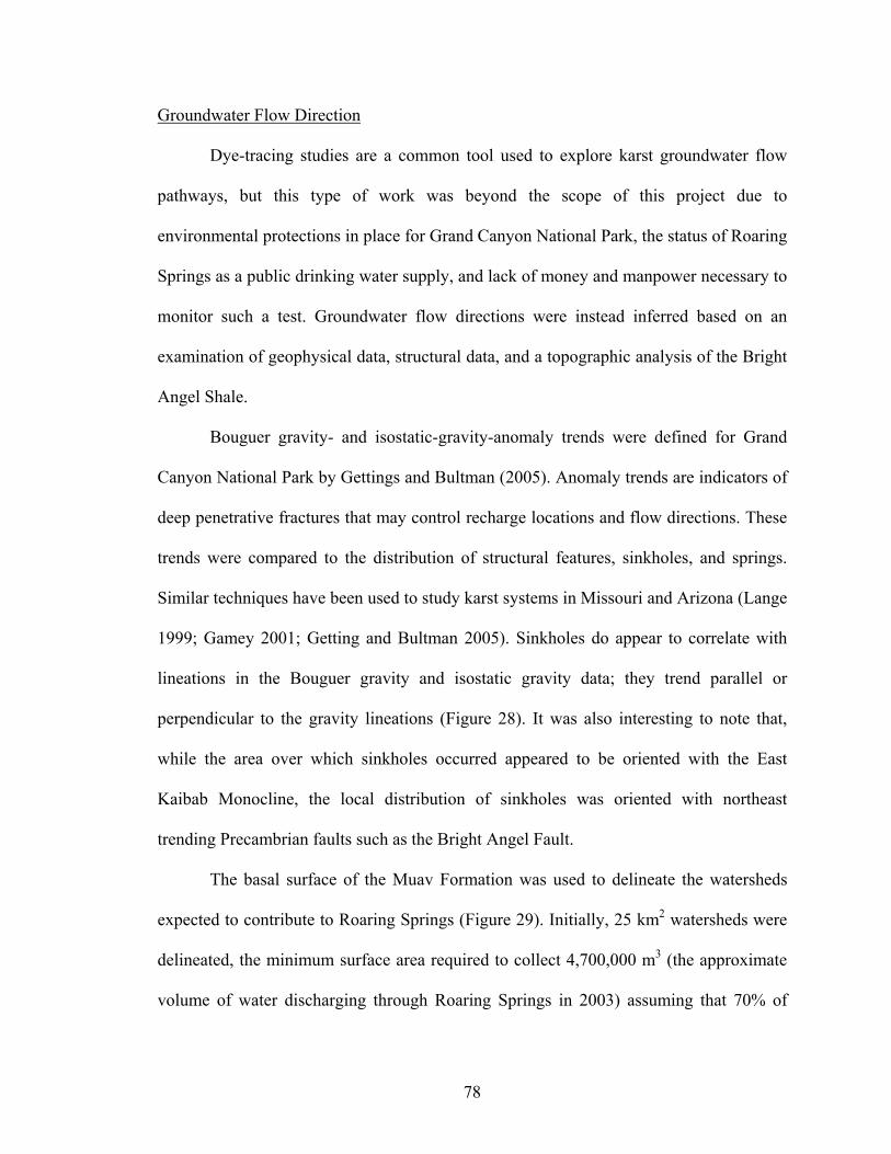
78
Groundwater Flow Direction
Dye-tracing studies are a common tool used to explore karst groundwater flow
pathways, but this type of work was beyond the scope of this project due to
environmental protections in place for Grand Canyon National Park, the status of Roaring
Springs as a public drinking water supply, and lack of money and manpower necessary to
monitor such a test. Groundwater flow directions were instead inferred based on an
examination of geophysical data, structural data, and a topographic analysis of the Bright
Angel Shale.
Bouguer gravity- and isostatic-gravity-anomaly trends were defined for Grand
Canyon National Park by Gettings and Bultman (2005). Anomaly trends are indicators of
deep penetrative fractures that may control recharge locations and flow directions. These
trends were compared to the distribution of structural features, sinkholes, and springs.
Similar techniques have been used to study karst systems in Missouri and Arizona (Lange
1999; Gamey 2001; Getting and Bultman 2005). Sinkholes do appear to correlate with
lineations in the Bouguer gravity and isostatic gravity data; they trend parallel or
perpendicular to the gravity lineations (Figure 28). It was also interesting to note that,
while the area over which sinkholes occurred appeared to be oriented with the East
Kaibab Monocline, the local distribution of sinkholes was oriented with northeast
trending Precambrian faults such as the Bright Angel Fault.
The basal surface of the Muav Formation was used to delineate the watersheds
expected to contribute to Roaring Springs (Figure 29). Initially, 25 km2 watersheds were
delineated, the minimum surface area required to collect 4,700,000 m3 (the approximate
volume of water discharging through Roaring Springs in 2003) assuming that 70% of
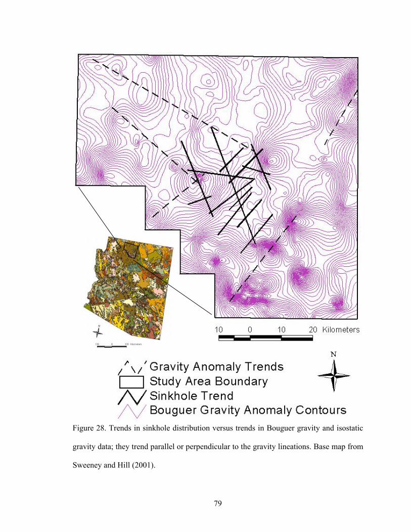
79
Figure 28. Trends in sinkhole distribution versus trends in Bouguer gravity and isostatic
gravity data; they trend parallel or perpendicular to the gravity lineations. Base map from
Sweeney and Hill (2001).
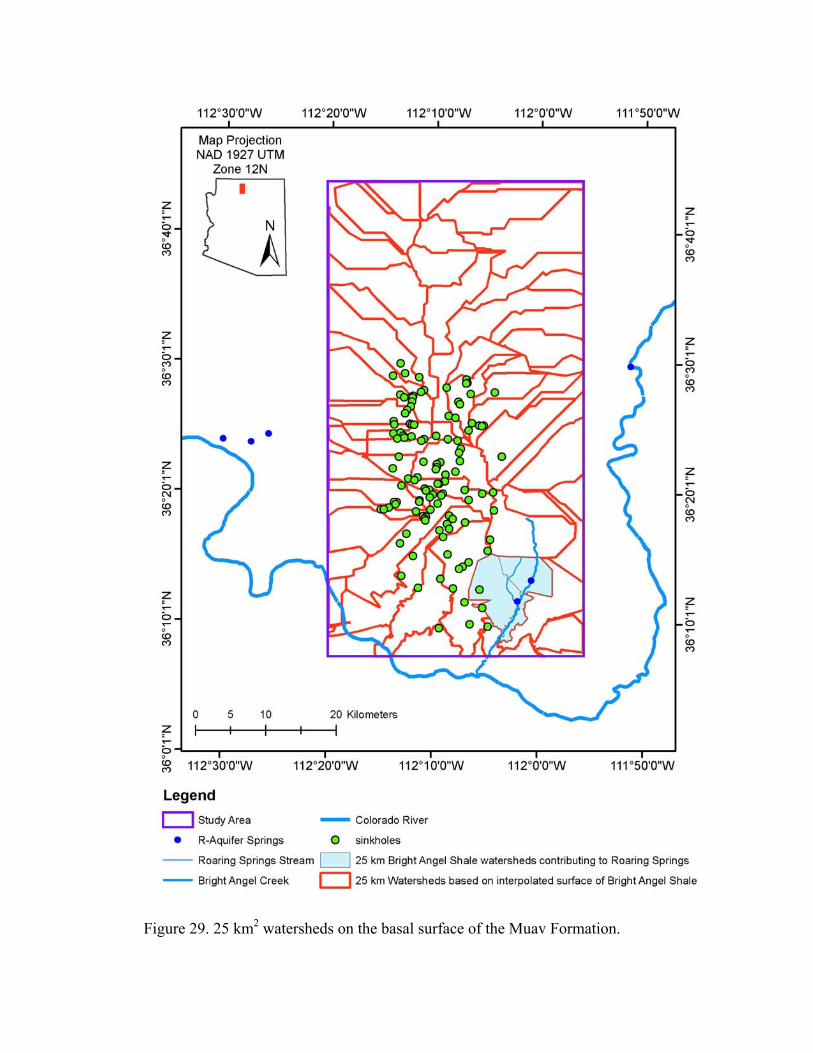
80
Figure 29. 25 km2 watersheds on the basal surface of the Muav Formation.
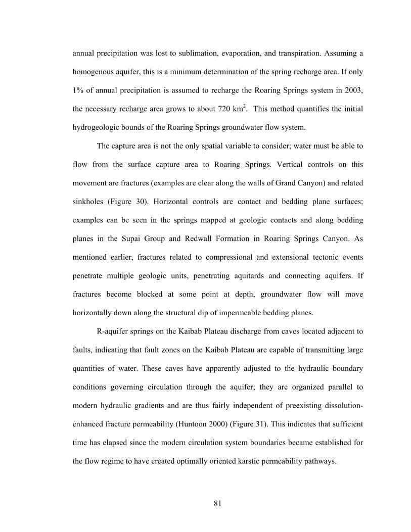
81
annual precipitation was lost to sublimation, evaporation, and transpiration. Assuming a
homogenous aquifer, this is a minimum determination of the spring recharge area. If only
1% of annual precipitation is assumed to recharge the Roaring Springs system in 2003,
the necessary recharge area grows to about 720 km2. This method quantifies the initial
hydrogeologic bounds of the Roaring Springs groundwater flow system.
The capture area is not the only spatial variable to consider; water must be able to
flow from the surface capture area to Roaring Springs. Vertical controls on this
movement are fractures (examples are clear along the walls of Grand Canyon) and related
sinkholes (Figure 30). Horizontal controls are contact and bedding plane surfaces;
examples can be seen in the springs mapped at geologic contacts and along bedding
planes in the Supai Group and Redwall Formation in Roaring Springs Canyon. As
mentioned earlier, fractures related to compressional and extensional tectonic events
penetrate multiple geologic units, penetrating aquitards and connecting aquifers. If
fractures become blocked at some point at depth, groundwater flow will move
horizontally down along the structural dip of impermeable bedding planes.
R-aquifer springs on the Kaibab Plateau discharge from caves located adjacent to
faults, indicating that fault zones on the Kaibab Plateau are capable of transmitting large
quantities of water. These caves have apparently adjusted to the hydraulic boundary
conditions governing circulation through the aquifer; they are organized parallel to
modern hydraulic gradients and are thus fairly independent of preexisting dissolution-
enhanced fracture permeability (Huntoon 2000) (Figure 31). This indicates that sufficient
time has elapsed since the modern circulation system boundaries became established for
the flow regime to have created optimally oriented karstic permeability pathways.
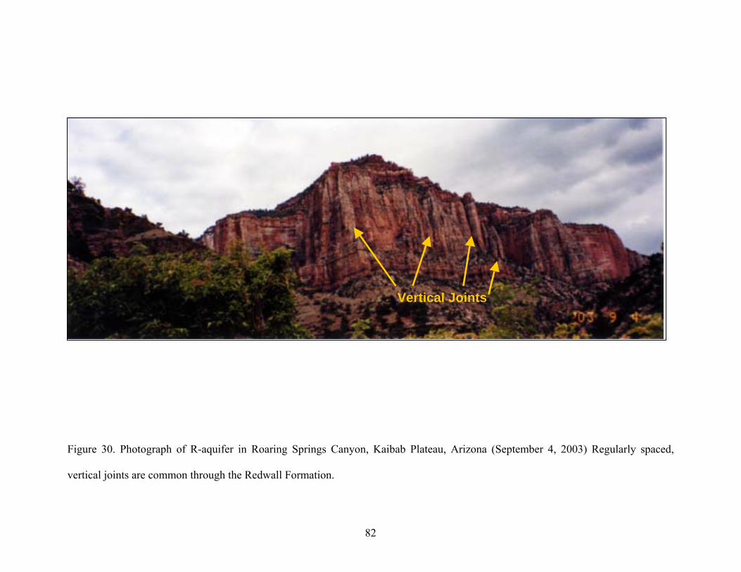
82
Figure 30. Photograph of R-aquifer in Roaring Springs Canyon, Kaibab Plateau, Arizona (September 4, 2003) Regularly spaced,
vertical joints are common through the Redwall Formation.
Vertical Joints
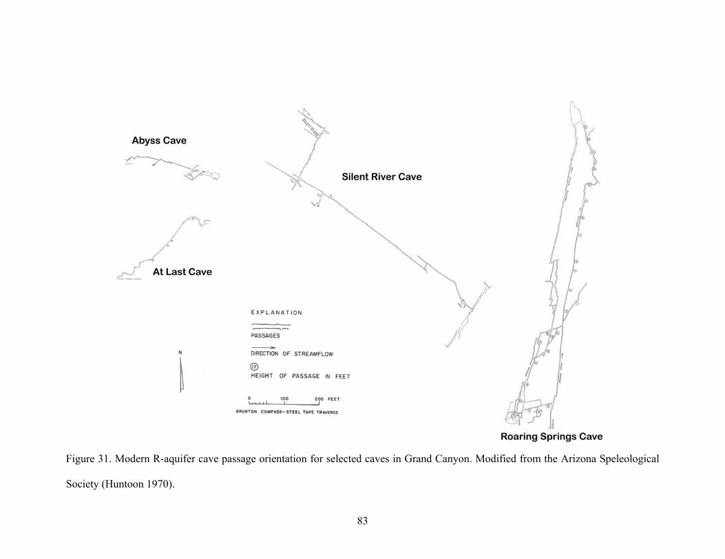
83
Figure 31. Modern R-aquifer cave passage orientation for selected caves in Grand Canyon. Modified from the Arizona Speleological
Society (Huntoon 1970).
84
Groundwater Flow Rates
The age of water discharging through Roaring Springs was determined as a mean
groundwater residence time, a value which reflects the likely mixture of modern and
older inputs in the aquifer. Only in well-defined and usually regional artesian aquifers
will true age gradients along the flow path be preserved (Clark and Fritz 1997). Evidence
of even small amounts of modern recharge was noted, however, because of its serious
implications for contaminant pathways. Groundwater flow rates through the R-aquifer
were estimated based on spring hydrograph analysis, oxygen and hydrogen stable isotope
analyses, and tritium age dating.
Previous to this study, documentation of spring response to precipitation events
was purely anecdotal (Johnson and Sanderson 1968; Huntoon 1970; Rihs 2002; Aiken
2003; Ross 2003). Pressure transducers installed in Roaring Springs Canyon monitored
water levels at 1 – 15 minute increments between March 8 and December 28, 2003. As
determined previously, this dataset quantifies the response time of the spring to recharge
events (Figure 23). Based on this figure, the spring responds to precipitation on the
Kaibab Plateau between 1 and 6 days. This conclusion assumes: peaks in the spring
hydrograph are due to increased flow and not due to head changes caused by barometric
pressure changes, that water discharging from the springs is the same water that fell as
precipitation, and that precipitation recorded at the Bright Angel Ranger Station on the
southern Kaibab Plateau represents the timing of precipitation in the nearby Roaring
Springs recharge area.
Recharge processes attenuate seasonal variations in δ18O and δ2H, and this rate of
attenuation has been found to be proportional to the length of groundwater flow paths,
85
and, consequently, to time (Raeisi and Karami 1997; Clark and Fritz 1997; Davisson
2000; Long and Putnam 2002). The preservation of any seasonal variation signifies short-
term mean residence times. When the pattern of stable isotope variability is compared to
spring discharge, it exhibits a seasonal variation. It also appears that recharge from
snowmelt reaches the spring in less than a month’s time (Figure 32). This conclusion is
also supported by an examination of the seasonal variation of Roaring Springs
temperature, pH, and specific conductivity (Figure 33).
The radiogenic isotope hydrogen, tritium (3H), can be incorporated in water
molecules and may be used to determine groundwater age, which can be used to infer
travel times along ground-water flow paths. This method has historically relied on the use
of the “bomb” signal, which was a peak in atmospheric tritium levels during
thermonuclear testing between 1952 and 1969 (Hart et al 2002b). By 1990, most bomb
tritium had been washed from the atmosphere, and tritium levels in global precipitation
are now close to natural levels. While thermonuclear tritium can still be found in some
slowly moving groundwater, the largely natural 3H signal is now relied upon for dating
modern groundwater. Natural tritium is formed in the upper atmosphere from the
bombardment of nitrogen by the flux of neutrons in cosmic radiation. The amount of
tritium in the atmosphere (precipitation) is a function of latitude; greater production
occurs at higher latitudes. The few measurements of natural pre-bomb tritium in
precipitation indicate that 3.4 - 6.6 TU is appropriate for latitudes corresponding to
Naples New York, and the Bordeaux and Rhone regions of France (Clarke and Fritz
1997). Water samples collected at Roaring Springs were analyzed for tritium to
qualitatively and quantitatively estimate a mean groundwater residence time.
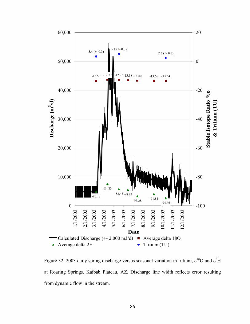
86
-12.77 -12.76-13.18 -13.40 -13.65 -13.54
-90.18
-84.83-88.43-88.82
-93.28 -91.84-94.66
-13.50
2.3 (+- 0.3)5.1 (+- 0.3)
3.4 (+- 0.3)
0
10,000
20,000
30,000
40,000
50,000
60,000
1/1/
2003
2/1/
2003
3/1/
2003
4/1/
2003
5/1/
2003
6/1/
2003
7/1/
2003
8/1/
2003
9/1/
2003
10/1
/200
3
11/1
/200
3
12/1
/200
3
Date
Dis
char
ge (m
3 /d)
-100
-80
-60
-40
-20
0
20
Stab
le Is
otop
e R
atio
%o
& T
ritiu
m (T
U)
Calculated Discharge (+- 2,000 m3/d) Average delta 18OAverage delta 2H Tritium (TU)
Figure 32. 2003 daily spring discharge versus seasonal variation in tritium, δ18O and δ2H
at Roaring Springs, Kaibab Plateau, AZ. Discharge line width reflects error resulting
from dynamic flow in the stream.
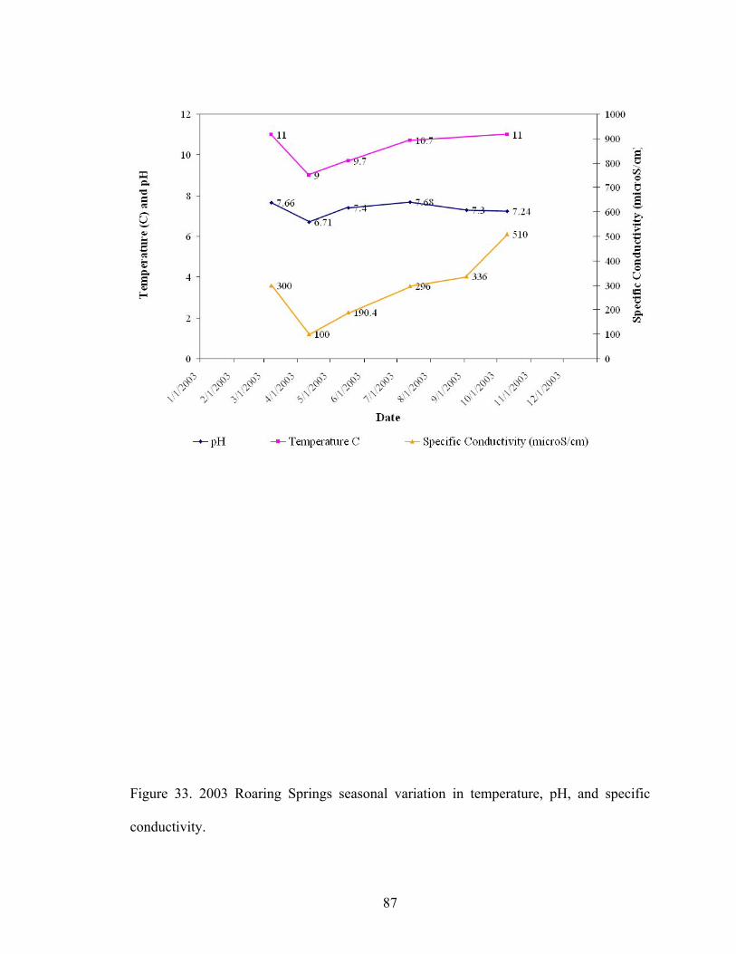
87
Figure 33. 2003 Roaring Springs seasonal variation in temperature, pH, and specific
conductivity.
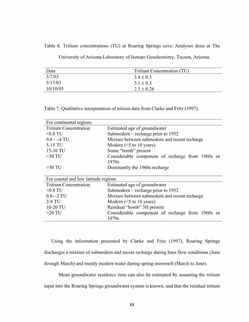
88
Table 6. Tritium concentrations (TU) at Roaring Springs cave. Analyses done at The
University of Arizona Laboratory of Isotope Geochemistry, Tucson, Arizona.
Date Tritium Concentration (TU) 3/7/03 3.4 ± 0.3 5/17/03 5.1 ± 0.3 10/10/03 2.3 ± 0.28
Table 7. Qualitative interpretation of tritium data from Clarke and Fritz (1997).
For continental regions Tritium Concentration Estimated age of groundwater <0.8 TU Submodern – recharge prior to 1952 0.8 - ~4 TU Mixture between submodern and recent recharge 5-15 TU Modern (<5 to 10 years) 15-30 TU Some “bomb” present >30 TU Considerable component of recharge from 1960s or
1970s >50 TU Dominantly the 1960s recharge For coastal and low latitude regions Tritium Concentration Estimated age of groundwater <0.8 TU Submodern – recharge prior to 1952 0.8-~2 TU Mixture between submodern and recent recharge 2-8 TU Modern (<5 to 10 years) 10-20 TU Residual “bomb” 3H present >20 TU Considerable component of recharge from 1960s or
1970s
Using the information presented by Clarke and Fritz (1997), Roaring Springs
discharges a mixture of submodern and recent recharge during base flow conditions (June
through March) and mostly modern water during spring snowmelt (March to June).
Mean groundwater residence time can also be estimated by assuming the tritium
input into the Roaring Springs groundwater system is known, and that the residual tritium
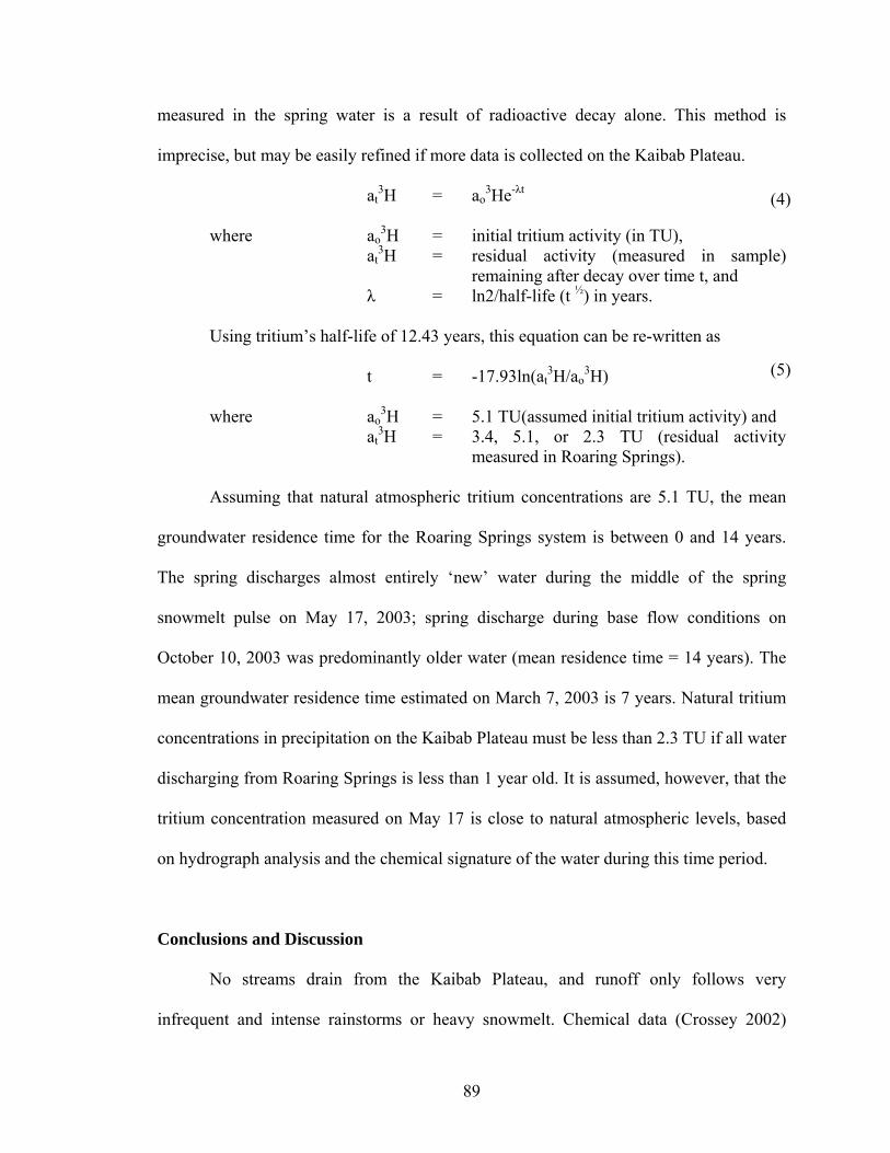
89
measured in the spring water is a result of radioactive decay alone. This method is
imprecise, but may be easily refined if more data is collected on the Kaibab Plateau.
at3H = ao
3He-λt
where ao3H = initial tritium activity (in TU),
at3H = residual activity (measured in sample)
remaining after decay over time t, and λ = ln2/half-life (t ½) in years.
Using tritium’s half-life of 12.43 years, this equation can be re-written as
t = -17.93ln(at3H/ao
3H)
where ao3H = 5.1 TU(assumed initial tritium activity) and
at3H = 3.4, 5.1, or 2.3 TU (residual activity
measured in Roaring Springs).
Assuming that natural atmospheric tritium concentrations are 5.1 TU, the mean
groundwater residence time for the Roaring Springs system is between 0 and 14 years.
The spring discharges almost entirely ‘new’ water during the middle of the spring
snowmelt pulse on May 17, 2003; spring discharge during base flow conditions on
October 10, 2003 was predominantly older water (mean residence time = 14 years). The
mean groundwater residence time estimated on March 7, 2003 is 7 years. Natural tritium
concentrations in precipitation on the Kaibab Plateau must be less than 2.3 TU if all water
discharging from Roaring Springs is less than 1 year old. It is assumed, however, that the
tritium concentration measured on May 17 is close to natural atmospheric levels, based
on hydrograph analysis and the chemical signature of the water during this time period.
Conclusions and Discussion
No streams drain from the Kaibab Plateau, and runoff only follows very
infrequent and intense rainstorms or heavy snowmelt. Chemical data (Crossey 2002)
(4)
(5)
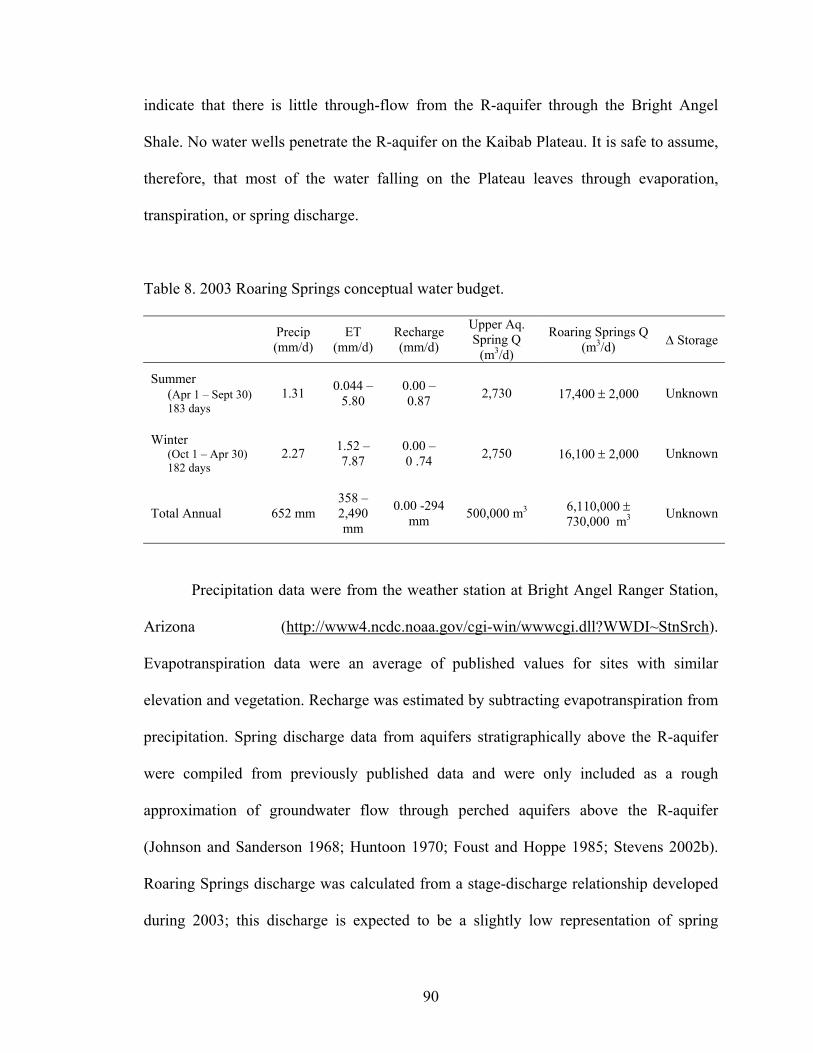
90
indicate that there is little through-flow from the R-aquifer through the Bright Angel
Shale. No water wells penetrate the R-aquifer on the Kaibab Plateau. It is safe to assume,
therefore, that most of the water falling on the Plateau leaves through evaporation,
transpiration, or spring discharge.
Table 8. 2003 Roaring Springs conceptual water budget.
Precip (mm/d)
ET (mm/d)
Recharge (mm/d)
Upper Aq. Spring Q
(m3/d)
Roaring Springs Q (m3/d) Δ Storage
Summer (Apr 1 – Sept 30) 183 days
1.31 0.044 – 5.80
0.00 – 0.87 2,730 17,400 ± 2,000 Unknown
Winter (Oct 1 – Apr 30) 182 days
2.27 1.52 – 7.87
0.00 – 0 .74 2,750 16,100 ± 2,000 Unknown
Total Annual 652 mm 358 – 2,490 mm
0.00 -294 mm 500,000 m3 6,110,000 ±
730,000 m3 Unknown
Precipitation data were from the weather station at Bright Angel Ranger Station,
Arizona (http://www4.ncdc.noaa.gov/cgi-win/wwwcgi.dll?WWDI~StnSrch).
Evapotranspiration data were an average of published values for sites with similar
elevation and vegetation. Recharge was estimated by subtracting evapotranspiration from
precipitation. Spring discharge data from aquifers stratigraphically above the R-aquifer
were compiled from previously published data and were only included as a rough
approximation of groundwater flow through perched aquifers above the R-aquifer
(Johnson and Sanderson 1968; Huntoon 1970; Foust and Hoppe 1985; Stevens 2002b).
Roaring Springs discharge was calculated from a stage-discharge relationship developed
during 2003; this discharge is expected to be a slightly low representation of spring
91
discharge as 2003 precipitation of 527 mm was slightly below average. Change in storage
can not be calculated until the aquifer extent is better defined.
Approximately 60% of recharge flows through the system almost immediately
after entering the aquifer, while 40% of annual recharge flows more slowly through the
aquifer and supports base flow out of the aquifer. This distribution of conduit and diffuse
flow is common in karst systems (White 2002).
The recharge area for Roaring Springs must be at least 25 km2 and is most likely
much larger. A topographic analysis of the Bright Angel Shale indicates that the northern
boundary of the Roaring Springs recharge area is likely located at a latitude of 36°20’,
approximately 16 km north of Roaring Springs.
Estimates of flow rate through the Roaring Springs groundwater system vary
between 1 day and >14 years, indicating that all water discharging from the aquifer is
relatively young and susceptible to rapid impacts from land-use activities on the Kaibab
Plateau. The range in flow rates reflects the diverse flow regimes present in the karst
aquifer. Rapid flow occurs through conduits while diffuse flow occurs in fractures,
partings, and intergranular pores.
Building a conceptual model of the Roaring Springs groundwater system depends
upon a multidisciplinary approach. Many of the datasets used in this study are lean, and
calculations based on these data have a significant level of uncertainty. The results
presented here are estimates that will be used as the initial parameters for the numerical
groundwater flow model developed in Chapter 4.
The conceptual model for the Roaring Springs groundwater flow system will
benefit from the collection of additional field data. Frequent, seasonal discharge
92
measurements at the Roaring Springs picnic area, which is above the main spring
complex, could quantify diffuse flow through the aquifer. Additional discharge
measurements immediately downstream of Roaring Springs would also be useful.
Installing a semi-permanent pressure transducer capable of collecting pressure,
temperature, and specific conductivity data in Roaring Springs cave would be an
inexpensive and valuable tool for understanding head changes and flow rates in the
aquifer.
Additional precipitation samples should be collected on the Kaibab Plateau and at
Roaring Springs for hydrogen and oxygen stable isotope and tritium analysis. If these
samples are collected over at least a year, a number of methods may be used to determine
mean groundwater residence times (Clark and Fritz 1997). The precipitation data would
also be useful to groundwater studies across the region. Bi-monthly or higher frequency
sampling is preferred.
93
CHAPTER 4
NUMERICAL GROUNDWATER FLOW MODEL
Purpose and Objectives
The Grand Canyon National Park has expressed an interest in developing a high-
quality map of spring recharge areas to determine if these areas fall inside or outside of
Park jurisdiction (Rihs 2002). This is a difficult task in a karst setting, but numerical
groundwater flow modeling methods have been adapted to this purpose. The karst
conduit system of Grand Canyon has not been well mapped, but other karst regions (such
as Kentucky) have been numerically modeled using a ‘black box’ approach (Anderson
and Woessner 1992). In this approach, functions are developed to reproduce recharge and
spring flow; this is the approach used in this study. The model developed in this study is
designed to define certain constraints on the Roaring Springs flow system (Anderson and
Woessner 1992).
The numerical groundwater flow model of the Roaring Springs flow system was
designed as an interpretive tool that organizes hydrogeologic field data and provides a
mathematical framework for studying the groundwater system, including the location of
groundwater sources, generalized flow paths, and flow boundaries. A numerical
groundwater flow model was chosen over an analytical model because analytical models
may oversimplify a problem, and they usually assume a homogenous porous medium.
The data in the numerical groundwater flow model was taken from the DGFM
and conceptual models developed for this study. The model was calibrated to the field
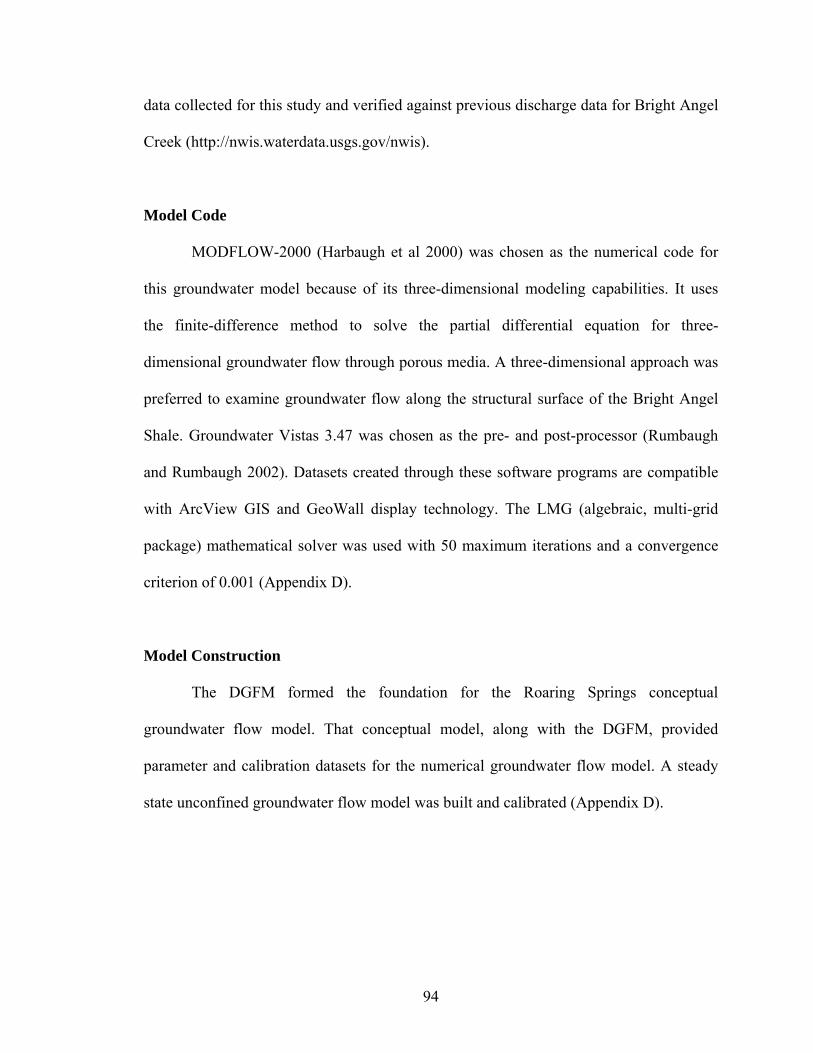
94
data collected for this study and verified against previous discharge data for Bright Angel
Creek (http://nwis.waterdata.usgs.gov/nwis).
Model Code
MODFLOW-2000 (Harbaugh et al 2000) was chosen as the numerical code for
this groundwater model because of its three-dimensional modeling capabilities. It uses
the finite-difference method to solve the partial differential equation for three-
dimensional groundwater flow through porous media. A three-dimensional approach was
preferred to examine groundwater flow along the structural surface of the Bright Angel
Shale. Groundwater Vistas 3.47 was chosen as the pre- and post-processor (Rumbaugh
and Rumbaugh 2002). Datasets created through these software programs are compatible
with ArcView GIS and GeoWall display technology. The LMG (algebraic, multi-grid
package) mathematical solver was used with 50 maximum iterations and a convergence
criterion of 0.001 (Appendix D).
Model Construction
The DGFM formed the foundation for the Roaring Springs conceptual
groundwater flow model. That conceptual model, along with the DGFM, provided
parameter and calibration datasets for the numerical groundwater flow model. A steady
state unconfined groundwater flow model was built and calibrated (Appendix D).
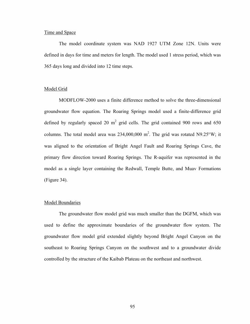
95
Time and Space
The model coordinate system was NAD 1927 UTM Zone 12N. Units were
defined in days for time and meters for length. The model used 1 stress period, which was
365 days long and divided into 12 time steps.
Model Grid
MODFLOW-2000 uses a finite difference method to solve the three-dimensional
groundwater flow equation. The Roaring Springs model used a finite-difference grid
defined by regularly spaced 20 m2 grid cells. The grid contained 900 rows and 650
columns. The total model area was 234,000,000 m2. The grid was rotated N9.25°W; it
was aligned to the orientation of Bright Angel Fault and Roaring Springs Cave, the
primary flow direction toward Roaring Springs. The R-aquifer was represented in the
model as a single layer containing the Redwall, Temple Butte, and Muav Formations
(Figure 34).
Model Boundaries
The groundwater flow model grid was much smaller than the DGFM, which was
used to define the approximate boundaries of the groundwater flow system. The
groundwater flow model grid extended slightly beyond Bright Angel Canyon on the
southeast to Roaring Springs Canyon on the southwest and to a groundwater divide
controlled by the structure of the Kaibab Plateau on the northeast and northwest.
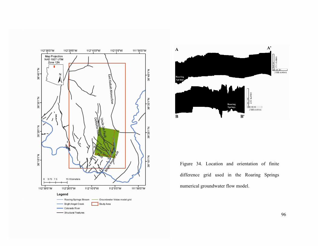
96
Figure 34. Location and orientation of finite
difference grid used in the Roaring Springs
numerical groundwater flow model.
96
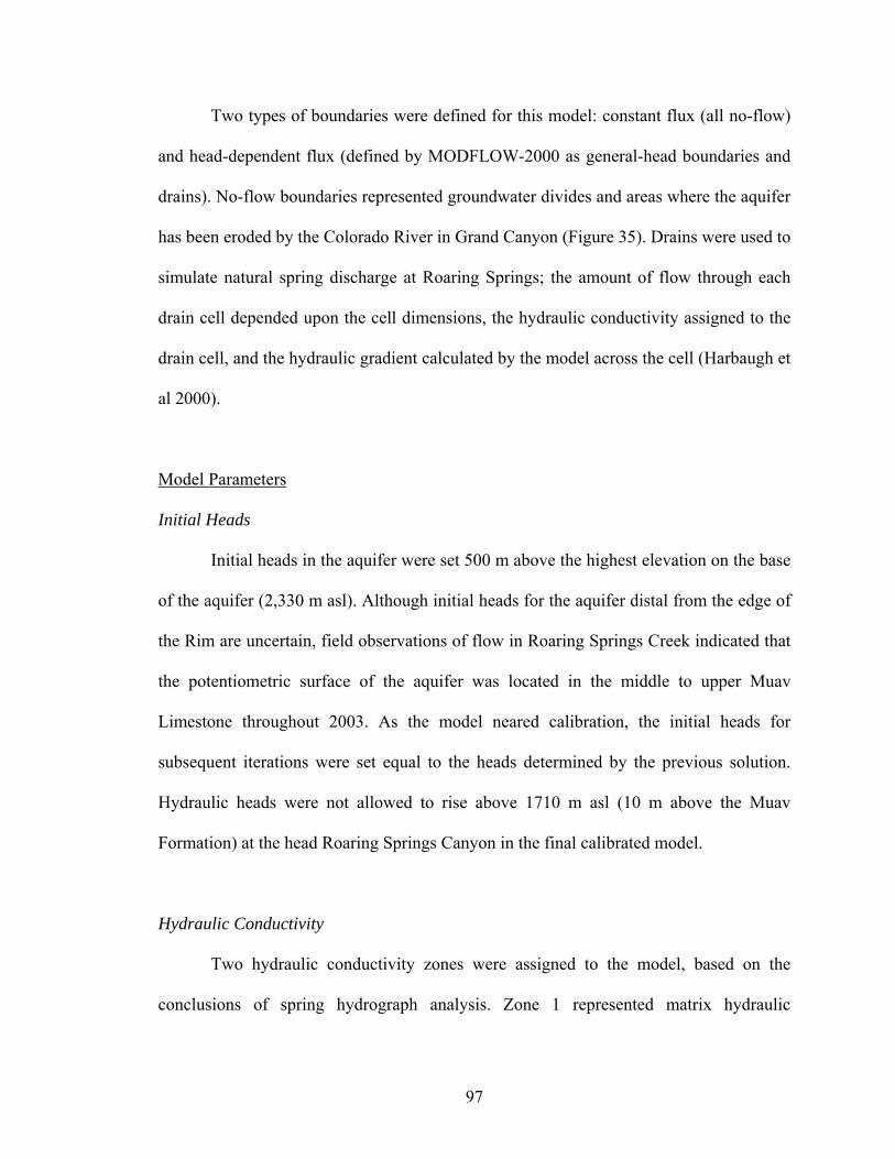
97
Two types of boundaries were defined for this model: constant flux (all no-flow)
and head-dependent flux (defined by MODFLOW-2000 as general-head boundaries and
drains). No-flow boundaries represented groundwater divides and areas where the aquifer
has been eroded by the Colorado River in Grand Canyon (Figure 35). Drains were used to
simulate natural spring discharge at Roaring Springs; the amount of flow through each
drain cell depended upon the cell dimensions, the hydraulic conductivity assigned to the
drain cell, and the hydraulic gradient calculated by the model across the cell (Harbaugh et
al 2000).
Model Parameters
Initial Heads
Initial heads in the aquifer were set 500 m above the highest elevation on the base
of the aquifer (2,330 m asl). Although initial heads for the aquifer distal from the edge of
the Rim are uncertain, field observations of flow in Roaring Springs Creek indicated that
the potentiometric surface of the aquifer was located in the middle to upper Muav
Limestone throughout 2003. As the model neared calibration, the initial heads for
subsequent iterations were set equal to the heads determined by the previous solution.
Hydraulic heads were not allowed to rise above 1710 m asl (10 m above the Muav
Formation) at the head Roaring Springs Canyon in the final calibrated model.
Hydraulic Conductivity
Two hydraulic conductivity zones were assigned to the model, based on the
conclusions of spring hydrograph analysis. Zone 1 represented matrix hydraulic
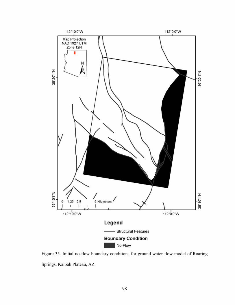
98
Figure 35. Initial no-flow boundary conditions for ground water flow model of Roaring
Springs, Kaibab Plateau, AZ.
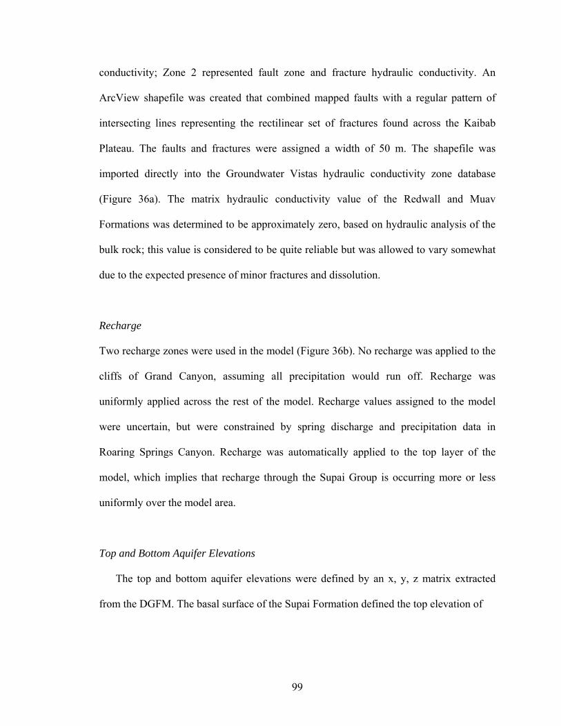
99
conductivity; Zone 2 represented fault zone and fracture hydraulic conductivity. An
ArcView shapefile was created that combined mapped faults with a regular pattern of
intersecting lines representing the rectilinear set of fractures found across the Kaibab
Plateau. The faults and fractures were assigned a width of 50 m. The shapefile was
imported directly into the Groundwater Vistas hydraulic conductivity zone database
(Figure 36a). The matrix hydraulic conductivity value of the Redwall and Muav
Formations was determined to be approximately zero, based on hydraulic analysis of the
bulk rock; this value is considered to be quite reliable but was allowed to vary somewhat
due to the expected presence of minor fractures and dissolution.
Recharge
Two recharge zones were used in the model (Figure 36b). No recharge was applied to the
cliffs of Grand Canyon, assuming all precipitation would run off. Recharge was
uniformly applied across the rest of the model. Recharge values assigned to the model
were uncertain, but were constrained by spring discharge and precipitation data in
Roaring Springs Canyon. Recharge was automatically applied to the top layer of the
model, which implies that recharge through the Supai Group is occurring more or less
uniformly over the model area.
Top and Bottom Aquifer Elevations
The top and bottom aquifer elevations were defined by an x, y, z matrix extracted
from the DGFM. The basal surface of the Supai Formation defined the top elevation of
100
Figure 36. Maps showing the distribution of hydraulic conductivity (A) and recharge values (B) in the groundwater flow model of
Roaring Springs, Kaibab Plateau, AZ.
A B
Recharge (m/d)
101
Layer 1. The basal surface of the Muav Limestone was the bottom elevation of Layer 1.
The elevation of the aquifer top and bottom was known with some certainty (Chapter 2).
Model Calibration
The model was loosely calibrated to hydraulic head at 2 locations in Roaring
Springs Canyon. Calibration targets were based on annual discharge calculations for both
Bright Angel Creek and Roaring Springs Canyon from 1923 to 1993, and 2003
(http://nwis.waterdata.usgs.gov/nwis/) (Ross 2003).
Calibration Targets
The model was calibrated to total annual spring discharge at Roaring Springs. The
annual water budget was allowed to vary between 80,400 m3/yr (Roaring Springs picnic
area discharge during base flow conditions) and 375,000,000 m3/yr (Bright Angel Creek
discharge during peak recharge conditions). The target goal (based on discharge at
Roaring Springs) was between 8,280,000 m3/yr and 11,200,000 m3/yr (15% deviation of
average annual discharge).
Calibration Process
The model was calibrated to within the target goal of 15% deviation from average
annual discharge at Roaring Springs (Table 9). This was accomplished using a manual
trial-and-error adjustment of parameters. Boundary conditions and aquifer properties
were adjusted during successive simulations until the computed hydraulic head and
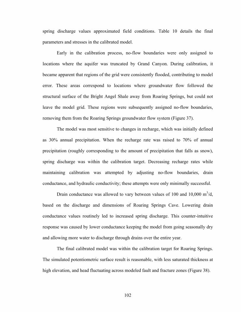
102
spring discharge values approximated field conditions. Table 10 details the final
parameters and stresses in the calibrated model.
Early in the calibration process, no-flow boundaries were only assigned to
locations where the aquifer was truncated by Grand Canyon. During calibration, it
became apparent that regions of the grid were consistently flooded, contributing to model
error. These areas correspond to locations where groundwater flow followed the
structural surface of the Bright Angel Shale away from Roaring Springs, but could not
leave the model grid. These regions were subsequently assigned no-flow boundaries,
removing them from the Roaring Springs groundwater flow system (Figure 37).
The model was most sensitive to changes in recharge, which was initially defined
as 30% annual precipitation. When the recharge rate was raised to 70% of annual
precipitation (roughly corresponding to the amount of precipitation that falls as snow),
spring discharge was within the calibration target. Decreasing recharge rates while
maintaining calibration was attempted by adjusting no-flow boundaries, drain
conductance, and hydraulic conductivity; these attempts were only minimally successful.
Drain conductance was allowed to vary between values of 100 and 10,000 m3/d,
based on the discharge and dimensions of Roaring Springs Cave. Lowering drain
conductance values routinely led to increased spring discharge. This counter-intuitive
response was caused by lower conductance keeping the model from going seasonally dry
and allowing more water to discharge through drains over the entire year.
The final calibrated model was within the calibration target for Roaring Springs.
The simulated potentiometric surface result is reasonable, with less saturated thickness at
high elevation, and head fluctuating across modeled fault and fracture zones (Figure 38).
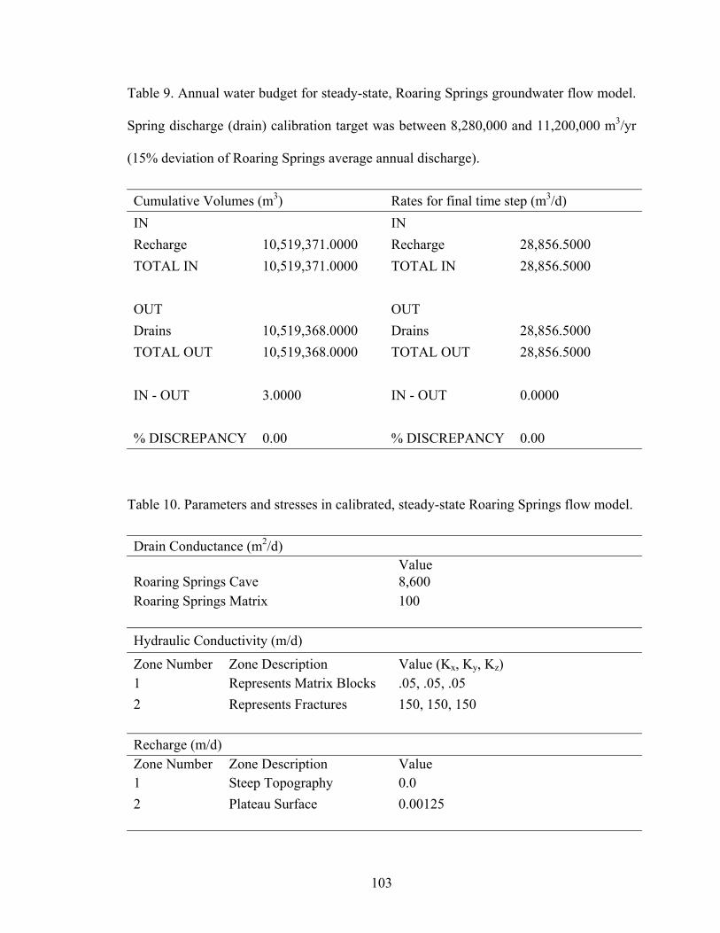
103
Table 9. Annual water budget for steady-state, Roaring Springs groundwater flow model.
Spring discharge (drain) calibration target was between 8,280,000 and 11,200,000 m3/yr
(15% deviation of Roaring Springs average annual discharge).
Cumulative Volumes (m3) Rates for final time step (m3/d) IN IN Recharge 10,519,371.0000 Recharge 28,856.5000 TOTAL IN 10,519,371.0000 TOTAL IN 28,856.5000 OUT OUT Drains 10,519,368.0000 Drains 28,856.5000 TOTAL OUT 10,519,368.0000 TOTAL OUT 28,856.5000 IN - OUT 3.0000 IN - OUT 0.0000 % DISCREPANCY 0.00 % DISCREPANCY 0.00
Table 10. Parameters and stresses in calibrated, steady-state Roaring Springs flow model.
Drain Conductance (m2/d) Value Roaring Springs Cave 8,600 Roaring Springs Matrix 100 Hydraulic Conductivity (m/d)
Zone Number Zone Description Value (Kx, Ky, Kz) 1 Represents Matrix Blocks .05, .05, .05 2 Represents Fractures 150, 150, 150 Recharge (m/d) Zone Number Zone Description Value 1 Steep Topography 0.0 2 Plateau Surface 0.00125
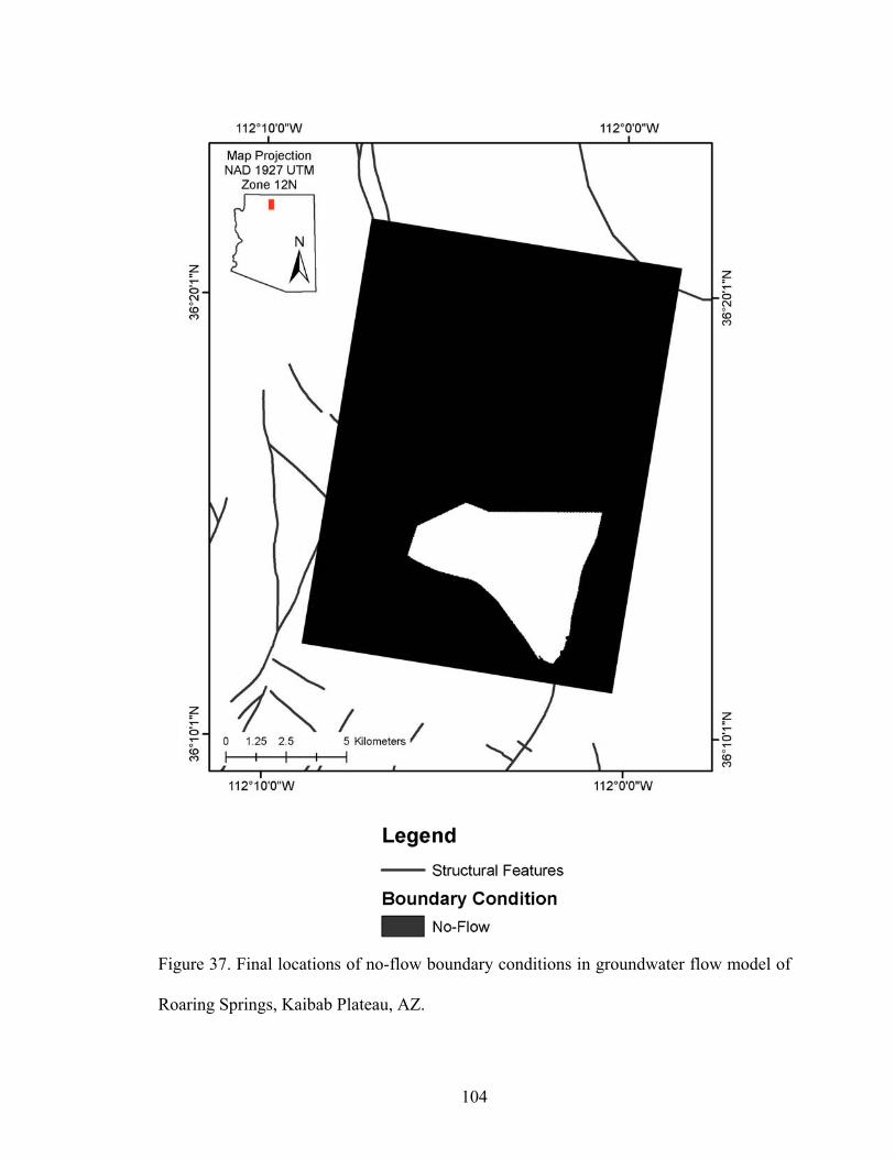
104
Figure 37. Final locations of no-flow boundary conditions in groundwater flow model of
Roaring Springs, Kaibab Plateau, AZ.
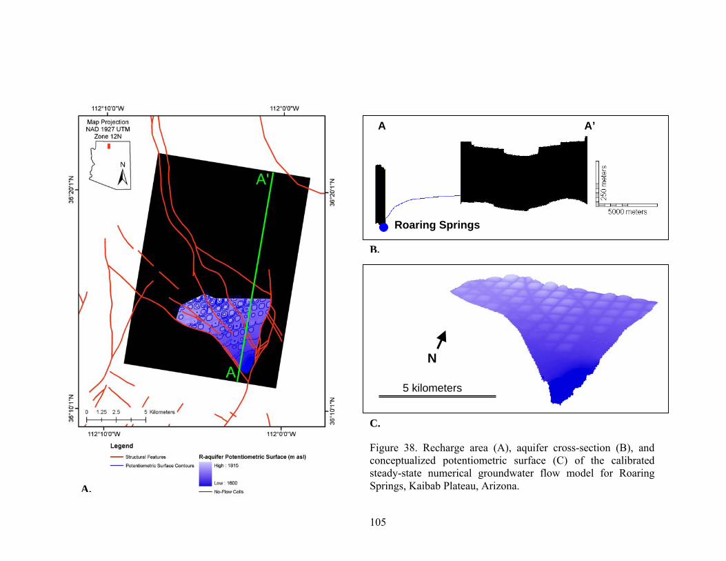
105
Figure 38. Recharge area (A), aquifer cross-section (B), andconceptualized potentiometric surface (C) of the calibratedsteady-state numerical groundwater flow model for RoaringSprings, Kaibab Plateau, Arizona.
105
A A’
Roaring Springs
N
5 kilometers
B.
C.
A.

106
Sensitivity Analysis
A model journal was kept to evaluate the calibration process. Based on a manual
trial-and-error sensitivity analysis, the model water budget was deemed most sensitive to
recharge volumes. The simulated water budget was deemed least sensitive to hydraulic
conductivity values assigned to the matrix and fractures. A sensitivity analysis was
conducted to better quantify model sensitivity to recharge and Roaring Springs drain
conductance values (Figure 39). The sensitivity analysis corroborates the conclusion that
the model water budget is most sensitive to recharge volumes. The model water budget is
least sensitive to the hydraulic conductivity values assigned to the aquifer matrix and
fractures. This conclusion realistically reflects the observed seasonal flux in spring
discharge due to seasonal recharge variability.
Varying fracture and matrix hydraulic conductivity did not impact the annual
water budget. These values primarily affect the relationship between flow in the matrix
and fractures, which controls the smoothness of the aquifer potentiometric surface. The
difference in hydraulic conductivity between the matrix and the fractures also affects the
expected chemical signature of spring discharge. The larger the volume of water held in
matrix blocks, the older the average ‘age’ of Roaring Springs discharge. Older water is
expected to contain greater concentrations of dissolved constituents. If the hydraulic
conductivity difference between matrix and fractures is smaller, flow will occur more
easily between them and differences in chemistry will be reduced. The model represented
the two different flow regimes of the Kaibab Plateau.
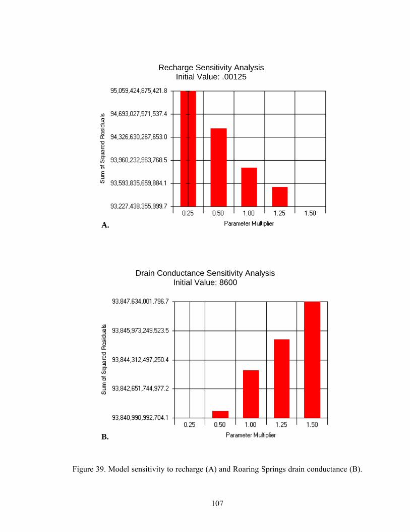
107
Figure 39. Model sensitivity to recharge (A) and Roaring Springs drain conductance (B).
Recharge Sensitivity Analysis Initial Value: .00125
Drain Conductance Sensitivity Analysis Initial Value: 8600
A.
B.
108
Model Limitations
This model is not intended for use as a predictive tool. It was constructed to
organize hydrogeologic field data and to illustrate the primary components of the Roaring
Springs groundwater system. This model demonstrates the volume of recharge required
to maintain spring flow, estimates hydraulic conductivity values of fractures, and defines
the general locations of groundwater divides.
Lack of data regarding the specific geometry of the conduit system in the R-
aquifer precluded the use of code written for discrete-fracture network models.
MODFLOW-2000 was chosen because it allowed the model to balance lack of data with
the inferred structural complexity of the plateau. While MODFLOW-2000 is an
equivalent porous media model, it can be adapted to function as a dual-continuum
formulation model. This problem has been examined by a variety of researchers who
concluded that MODFLOW-2000 generates reasonable results in karst terrains,
particularly when used to model spring discharge over a large area. MODFLOW-2000
should not be used to track particle flow through a karst aquifer because of the great
uncertainty in predicting the distribution of flow paths (Knochemnus and Robinson 1996,
Daniel et al 1997, Wilson 2000, Scanlon et al 2003).
Some assumptions made in the conceptual model were carried through to the
numerical model. When analyzing results of the numerical model, one should consider
the following subjects: how karstification and aquifer heterogeneity impact the
distribution of hydraulic conductivity; the assumption that Darcy’s law is applicable to
flow through the fractures and solutions openings in a karst region; the assumption that
little to no water is stored from one recharge event to the next in pools within the karst
109
system; and that the Bright Angel Shale is an effective confining layer and that little or no
water leaves the model through this unit.
Conclusions and Discussion
The calibrated model budget verifies that the R-aquifer within the conceptual
model boundaries is capable of sustaining field measured discharge to Roaring Springs,
although most of the winter snow pack is necessary for recharge. Under these conditions,
the Roaring Springs groundwater flow system is restricted to the Kaibab Plateau within
Grand Canyon National Park.
The model did not quantitatively define the flow pathways from the surface of the
Kaibab Plateau to Roaring Springs. This can only be addressed through tracer studies and
expanded mapping of the cave system.
The model should be improved by re-examining the conceptual model after more
data collection has occurred. The model may also be improved by expanding the
boundaries to include data from other springs, which would provide better calibration
potential. Future data collection should include many more spring discharge and aquifer
head measurements, particularly upstream of Roaring Springs. More data are also needed
regarding recharge rates in sinkholes and fractures on the Kaibab Plateau.
The process used in this project demonstrates the use of a preliminary model in an
interpretive sense and illustrates the strength of a groundwater flow model as a
framework for organizing available field data and for identifying deficiencies in the
existing database.
110
CHAPTER 5
SUMMARY AND DISCUSSION
Roaring Springs discharges from the unconfined, karstic, R-aquifer in the Kaibab
Plateau, Arizona. As the sole supply of drinking water to Grand Canyon National Park,
an assessment of the Roaring Springs recharge area and groundwater flow rate was
warranted. This study’s groundwater flow modeling methodology included the
construction of a digital geologic framework model, description of a conceptual model of
the Roaring Springs groundwater flow system, and the construction and calibration of a
numerical groundwater flow model.
Results indicate that almost 70% of annual precipitation (corresponding to the
volume of winter precipitation) is needed to recharge the R-aquifer and that recharge
occurs solely during the winter season. Recharging groundwater moves through the
aquifer along two principal pathways: 1) turbulent flow through structurally-controlled
dissolution enhanced conduits, and 2) diffuse laminar flow through small fractures, fault
gouge, and along bedding plane partings. These two flow regimes are apparent on the
Roaring Springs hydrograph base flow recession curves. Water flowing through the
conduit system moves from land surface to Roaring Springs in less than a month, likely
within a day. Water moving through the larger aquifer matrix moves more slowly, with
travel times ranging from months to years. Mean groundwater residence time is ~7 years,
based on tritium analysis of spring water.
The recharge area is constrained by the structural relief of the Bright Angel Shale,
the R-aquifer’s basal confining unit. The approximate recharge area is 30 km2. Aquifer
111
geometry can be easily displayed on the GeoWall, a three-dimensional visualization
technology designed to enhance understanding of complex geologic systems. The
GeoWall allows for rapid and simple identification of errors in geologic model
construction, especially for interpretive modeling exercises, such as this study.
The results presented above are based primarily on high-frequency stage
measurements made between March and December 2003 in Roaring Springs stream and
cave, hydrograph analysis of historical discharge data in Bright Angel Creek, watershed
modeling using a DGFM, and calibration of a numerical flow model.
Roaring Springs discharge and isotope data were collected to quantify the
response time of the aquifer to recharge events occurring on the Kaibab Plateau, to
determine the source of recharge, and to approximate mean groundwater residence time
in the aquifer. These data effectively quantified response time and identified the presence
of multiple flow paths, but more chemical data are needed to refine flow pathways.
Collection of precipitation and spring water samples over a full year would yield better
results. Collection of chemistry samples during and immediately after precipitation
events, late season sample collection, and sample collection above the main stream
complex would also improve understanding of matrix/diffuse flow processes.
A DGFM was constructed to define aquifer geometry. Available datasets
restricted accuracy of this geometry to scales greater than 1:100,000, but this scale is
adequate to assess groundwater flow bounds. The model would be improved by refined
mapping and development of improved interpolation methods. The DGFM illustrated the
dilemma of moving from paper to digital data; geologic mapping and model construction
will not be efficient until a more consistent digital mapping scheme is widely adopted.
112
The move to 3D digital geologic modeling will greatly benefit hydrogeologic research by
providing more reliable data.
Calibration of an interpretive numerical flow model was done to test the strength
of the conceptual model and to refine the Roaring Springs/Kaibab Plateau water budget.
MODFLOW-2000, the software program chosen, is appropriate for this purpose but is
not capable of predicting groundwater flow paths accurately. The model is deemed an
appropriate tool to improve our conceptual understanding of the system, although future
modeling (both numerical and analytical) will continue to improve our understanding of
Roaring Springs.
The final model was displayed with a GeoWall (a digital three-dimensional
projection system designed for classroom presentations) to test its applicability for
hydrologic education (Ross 2003; Fry and Springer 2005a, b). The digital geologic
framework model can be easily rotated and examined at different scales using this
system; the structure of the Kaibab Plateau is clearly illustrated. The recharge area and
potentiometric surface of the Roaring Springs groundwater system are too small,
however, to be viewed easily in the context of the Kaibab Plateau using the GeoWall. In
general, this method continues to improve with technological advances in geographic
information system software programs, but common challenges include computer
processing time needed to render detailed, large-scale, complex geological datasets,
educators and others’ lack of time and their unfamiliarity with visualization software
and/or GIS software, and lack of detailed technical resources for newly developed and
developing visualization software.
113
BIBLIOGRAPHY
Aiken, B., 2003, Personal communication, April 11. Anderson, M.P., and Woessner, W.W., 1992, Applied groundwater modeling; simulation of flow and advective transport: New York, Academic Press, 381 p. Beus, S.S., 1990a, Redwall Limestone and Surprise Canyon Formation, in Beus, S.S., and Morales, M., eds., Grand Canyon geology: New York, Oxford University Press, p. 119-145. Beus, S.S., 1990b, Temple Butte Formation, in Beus, S.S., and Morales, M., eds., Grand Canyon geology: New York, Oxford University Press, p. 107-117. Beus, S.S., and Morales, M., eds., 1990, Grand Canyon geology: New York, Oxford University Press, 518 p. Bills, D.J. and Flynn, M.E., 2002, Hydrogeologic data for the Coconino Plateau and adjacent areas, Coconino and Yavapai Counties, Arizona: U.S. Geological Survey Open File Report 02-265, 2192 p. Billingsley, G.H., and Hampton, H.M., 2000, Geologic map of the Grand Canyon 30' X 60' quadrangle, Coconino and Mohave Counties, northwestern Arizona: U.S. Geological Survey Geologic Investigations Series I-2688, scale 1:100,000, digital format, 17 p. text. Billingsley, G.H., and Hampton, H.M., 2001, Geologic map of the House Rock Spring quadrangle, Coconino County, northern Arizona: U. S. Geological Survey Miscellaneous Field Studies Map MF-2367, scale 1:24,000, digital format. Billingsley, G.H., and Wellmeyer, J.L., 2001a, Geologic map of the Cane quadrangle, Coconino County, northern Arizona: U. S. Geological Survey Miscellaneous Field Studies Map MF-2366, scale 1:24,000, digital format. Billingsley, G.H., and Wellmeyer, J.L., 2001b, Geologic map of the House Rock quadrangle, Coconino County, northern Arizona: U. S. Geological Survey Miscellaneous Field Studies Map MF-2364, scale 1:24,000, digital format. Blakey, R.C., 1990, Supai Group and Hermit Formation in Beus, S.S., and Morales, M., eds., Grand Canyon geology: New York, Oxford University Press, p. 147-182. Cepeda, J.C, 1994, Fracture orientation and distribution on the Kaibab Plateau: The Mountain Geologist, v. 31, p. 77-83.
114
Clark, I., and Fritz, P., 1997, Environmental isotopes in hydrogeology: Boca Raton, CRC Press LLC, 328 p. Crossey, L., 2002, Active springs and quaternary travertines in Grand Canyon: Linking modern and paleo-hydrologic systems: Geological Society of America Abstracts with Programs, no. 175-16, p. A101-A103.
Daniel, III, C.C., Smith, D.G., and Eimers, J.L., 1997, Hydrogeology and simulation of ground-water flow in the thick regolith-fractured crystalline rock aquifer system of Indian Creek basin, North Carolina in Ground-water resources of the Piedmont-Blue Ridge provinces of North Carolina: U.S. Geological Survey Water Supply Paper 2341-C, p. C1-C137.
Davisson, M.L., 2000, Summary of age-dating analysis in the Fenner Basin, Eastern Mojave Desert, California: Lawrence Livermore National Laboratory W-7405-Eng-48, 2 p. Diodato, D.M., 1994, A compendium of fracture flow models – 1994: Hohenfels, U.S. Department of Defense, 94 p. Drever, J.I., 1997, The geochemistry of natural waters: surface and groundwater environments, third edition: New Jersey, Prentice-Hall, Inc., 436 p. Fetter, C. W., 2001, Applied hydrogeology: Upper Saddle River, Prentice Hall, 597 p. Fry, M. and Springer A.E., 2005a, Using the GeoWall to visualize aquifers of Arizona in three dimensions, 18th Annual Symposium of the Arizona Hydrological Society, September 22-23, 2005, Flagstaff, AZ. Fry, M. and Springer, A.E., 2005b, 3-D visualization of aquifers of Arizona with the Geowall, Annual meeting of the Geological Society of America, October 16-19, 2005. Salt Lake City, UT. Foust, R. and Hoppe, S., 1985, Seasonal trends in the chemical composition of Grand Canyon waters: Flagstaff, Ralph M. Bilby Research Center, Northern Arizona University, 39 p. Gamey, T.J., 2001. Karst pathway delineation using combined spatial and geophysical analysis at Camp Crowder, Missouri in Proceedings, Geological Society of America Annual Meeting, 2001, Boston, MA, November 2001. Gettings, M.E. and Bultman, M.W., 2005, Candidate-penetrative-fracture mapping of the Grand Canyon Area, Arizona, from spatial correlation of deep geophysical features and surficial lineaments: U.S. Geologic Survey Data Series 121, 35 p.
115
Ginsberg, M. and Palmer, A., 2002, Delineation of source-water protection areas in karst aquifers of the Ridge and Valley and Appalachian Plateaus physiographic provinces: rules of thumb for estimating the capture zones of springs and wells: U.S. Environmental Protection Agency EPA 816-R-02-015, 51 p. Harbaugh, A.W., Banta, E.R., Hill, M.C., and McDonald, M.G., 2000, MODFLOW-2000, the U.S. Geological Survey modular ground-water model – user to modularization concepts and the ground-water flow process: U.S. Geological Survey Open-File Report 00-92, 121 p. Hart, R.J., Ward, J.J., Bills, D.J., and Flynn, M.E., 2002a, Generalized hydrogeology and ground-water budget for the C Aquifer, Little Colorado Basin and parts of the Verde and Salt River Basins, Arizona and New Mexico: U.S. Geological Survey Water Resources Investigations Report 02-4026, 54 p. Hart, R.J., Rihs, J., Taylor, H., Taylor, E., and Monroe, S.J., 2002b, Assessment of spring chemistry along the south rim of Grand Canyon in Grand Canyon National Park, Arizona: U.S. Geological Survey Fact Sheet 096-02, 4 p. Hereford, R, and Huntoon, P.W., 1990, Rock movement and mass wastage in the Grand Canyon in Beus, S.S., and Morales, M., eds., Grand Canyon geology: New York, Oxford University Press, p. 443-460. Hopkins, R.L., 1990 Kaibab Formation in Beus, S.S., and Morales, M., eds., Grand Canyon geology: New York, Oxford University Press, p. 225-245. Huntoon, P.W, 1970, The hydro-mechanics of the groundwater system in the southern portion of the Kaibab Plateau, Arizona [Ph.D. Dissertation]: Tucson, University of Arizona, 251 p. Huntoon, P.W., 1974, The karstic groundwater basins of the Kaibab Plateau, Arizona: Water Resource Research, v. 10, p. 579-590. Huntoon, P.W., 1990, Phanerozoic structural geology of the Grand Canyon, in Beus, S.S., and Morales, Michael, eds., Grand Canyon geology: New York, Oxford University Press, p. 261-309. Huntoon, P.W., 2000, Karstification associated with groundwater circulation through the Redwall artesian aquifer, Grand Canyon, Arizona, U.S.A., in Klimchouk, AB., Ford, D, C., Palmer, A, N., and Dreybrodt, W., eds., Speleogenesis: evolution of karst aquifers: Huntsville, National Speleological Society, Inc., p. 287-291. Huntoon, P.W., 2002, Written communication, September 22.
116
Johnson, P.S., 2000, Phase II hydrogeologic and water resource assessment for the Placitas development area, Sandoval County, New Mexico: Final technical report for county of Sandoval, New Mexico, January 30, 2000, 57 p. Johnson, P.W. and Sanderson, R.B., 1968, Spring flow into the Colorado River, Lees Ferry to Lake Mead, Arizona: Arizona State Lake Department of Water Resources Report 34, 26 p. Kessler, J., 2002, Grand Canyon Springs and the Redwall-Muav Aquifer: Comparison of Geologic Framework and Groundwater Flow Models [Master’s Thesis]: Flagstaff, Northern Arizona University, 122 p. Knochenmus, L.A. and Robinson, J.L., 1996, Descriptions of anisotropy and heterogeneity and their effect on ground-water flow and areas of contribution to public supply wells in a karst carbonate aquifer system: U.S. Geological Survey Water Supply Paper 2475, 54 p. Kobor, J., 2004, Simulating water availability in a spring-fed aquifer with surface water/groundwater flow models, Grand Canyon, Arizona [Master’s Thesis]: Flagstaff, Northern Arizona University, 141 p. Lange, A., 1999, Geophysical studies at Kartchner Caverns State Park, Arizona: Journal of Cave and Karst Studies, v. 61, no. 2, p. 68-72. Long, A.J. and Putnam, L.D., 2002, Evaluating travel times and transient mixing in a karst aquifer using time-series analysis of stable isotope data, in Proceedings, U.S. Geological Survey Karst Interest Group: Shepherdsdown, West Virginia, August 20-22, 2002. McKee, E.D., and Gutschick, R.C., 1969, The Redwall Limestone: Boulder, The Geological Society of America, 726 p. McKee, E.D., 1982, The Supai Group of Grand Canyon, USGS Professional Paper 1173, 504 p. Middleton, L.T. and Elliot, D. K., 1990, Tonto Group, in Beus, S.S., and Morales, Michael, eds., Grand Canyon geology: New York, Oxford University Press, p. 83-106. Miller, J.L., Springer, A.E., and Ross, L., 2004, The relationship of seasonal rainfall and recharge within the Grand Canyon's North Rim Redwall-Muav aquifer using 18O and 2H, 17th Annual Symposium of the Arizona Hydrological Society, September 16-17, 2004, Tucson, AZ. Montgomery and Associates, 1996, Assessment of the hydrologic conditions and potential effects of proposed ground water withdrawal for Canyon Forest Village,
117
Coconino County, Arizona in Appendix of the final environmental impact statement for Tusayan growth: Kaibab National Forest, 64 p. Monroe, S.A., Antweiler, R.J., Hart, R.J., Taylor, H.E., Truini, M., Rihs, J.R., and Felger, T.J., 2004, Chemical characteristics of ground-water discharge along the South Rim of Grand Canyon in Grand Canyon National Park, Arizona, 2000-2001: U.S. Geological Survey Scientific Investigations Report 2001-5146, 59 p. Parnell, R.A., 2005, Personal communication, November 21. Pierce, H.W. and Scurlock, J.R., 1972, Arizona well information: Arizona Bureau of Mine Bulletin 185, 195 p.
Quinlan, J.F., Smart, P.L., Schindel, G.M., Alexander, E.C., Edwards, A.J., and Smith, A.R., 1992, Recommended administrative/regulatory definition of karst aquifer, principles for classification of carbonate aquifers, practical evaluation of vulnerability of karst aquifers, and determination of optimum sampling frequency at springs, in Proceedings of the third conference on hydrogeology, ecology, monitoring, and management of ground water in karst terranes: Ground Water Management, v. 10, p. 573-635.
Quinn, J.J. and Tomasko, D., 2002, Numerical modeling of mixed-flow karst systems: approach and input data: Geological Society of America Abstracts with Programs, no. 98-4, poster. Raeisi, E. and Karami, G., 1997, Hydrochemographs of Beghan Karst Spring as indicators of aquifer characteristics: Journal of Cave and Karst Studies, v. 59, no. 3, p.112-118. Rantz, S.E., 1983, Measurement and computation of streamflow: Volume 1. Measurement of stage and discharge: USGS, Chapter 5, 80 p. Rihs, J., 2000, Spring related activities of the National Park Service, in Proceedings, Coconino Plateau Hydrology Workshop, 1st, Flagstaff: Arizona, Flagstaff Center for Sustainable Environments, p. 20-22. Rihs, J., 2002, Personal communication, January 7. Roller, J.A., 1987, Fracture history of the Redwall Limestone and lower Supai Group, western Hualapai Indian Reservation, northwestern Arizona: U.S. Geological Survey Open-File Report 87-359, 33 p. Ross, L.E., 2003, Three-dimensional groundwater modeling of the Redwall-Muav aquifer on the North Rim of Grand Canyon, Arizona, based on newly collected data sets: Geological Society of America Abstracts with Programs, v.35, no. 6, p. 373.
118
Rumbaugh, J.O. and Rumbaugh, D.B., 2002, Groundwater Vistas 3.47 Scanlon, B.R., Mace R.E., Barrett, M.E., and Smith, B., 2003, Can we simulate regional groundwater flow in a karst system using equivalent porous media models? Case study Barton Springs Edwards Aquifer, USA: Journal of Hydrology, v. 276, p. 137-158. Scurlock, J.R., 1973, Arizona Well information - Supplement 1: Arizona Oil and Gas Conservation Commission Report of Investigation Number Five, 28 p. Siska, P. and I-Kuai, H., 2001, Assessment of kriging accuracy in the GIS environment: Conference Proceedings, 21st Annual ESRI International User Conference, Sand Diego, California, 2001. Smith, B.A. and Hunt, B.B., 2004, Evaluation of sustainable yield of the Barton Springs segment of the Edwards Aquifer, Hays and Travis Counties: Barton Springs/Edwards Aquifer Conservation District, 71 p. Spence, J.R., 1999, Climate of the Central Colorado Plateau, Utah and Arizona: characterization and recent trends in Proceedings of the 5th Biennial Conference of Research on the Colorado Plateau: USGS Colorado Plateau Research Station, p. 187-203. Springer, A.E, Amentt, M.A., Kolb, T.E., and Mullen, R.M, In press, Evapotranspiration of two vegetation communities in a high-elevation riparian meadow at Hart Prairie, AZ. Water Resources Research. Stevens, L., 2001, An inventory, assessment, and development of recovery priorities for Arizona Strip springs, seeps and natural ponds: a synthesis of information: Arizona Water Protection Fund Grant Number 99-074WPF: Task 2, 53 p. Stevens, L, 2002a, Personal communication, January 1. Stevens, L., 2002b, A hydrogeochemical and biological inventory of springs on the Arizona Strip, Draft Final Report: Flagstaff, Grand Canyon Wildlands Council. Sweeney, R. and Hill, P., 2001, Arizona aeromagnetic and gravity maps and data, U.S. Geological Survey Open File Report 01-0081, scale 1:1,000,000, digital format. Tindall, S.E., 2000a, The Cockscomb segment of the East Kaibab monocline: Taking the structural plunge, in Sprinkel, D.A., Chidsey, T.C. and Anderson, P.B., eds., Geology of Utah's Parks and Monuments: Utah Geological Association Publication 28, p. 629-643. Tindall, S.E., 2000b, Development of oblique-slip basement-cored uplifts: Insights from the Kaibab Uplift and from physical models [Ph.D. dissertation]: Tucson, The University of Arizona, 261 p.
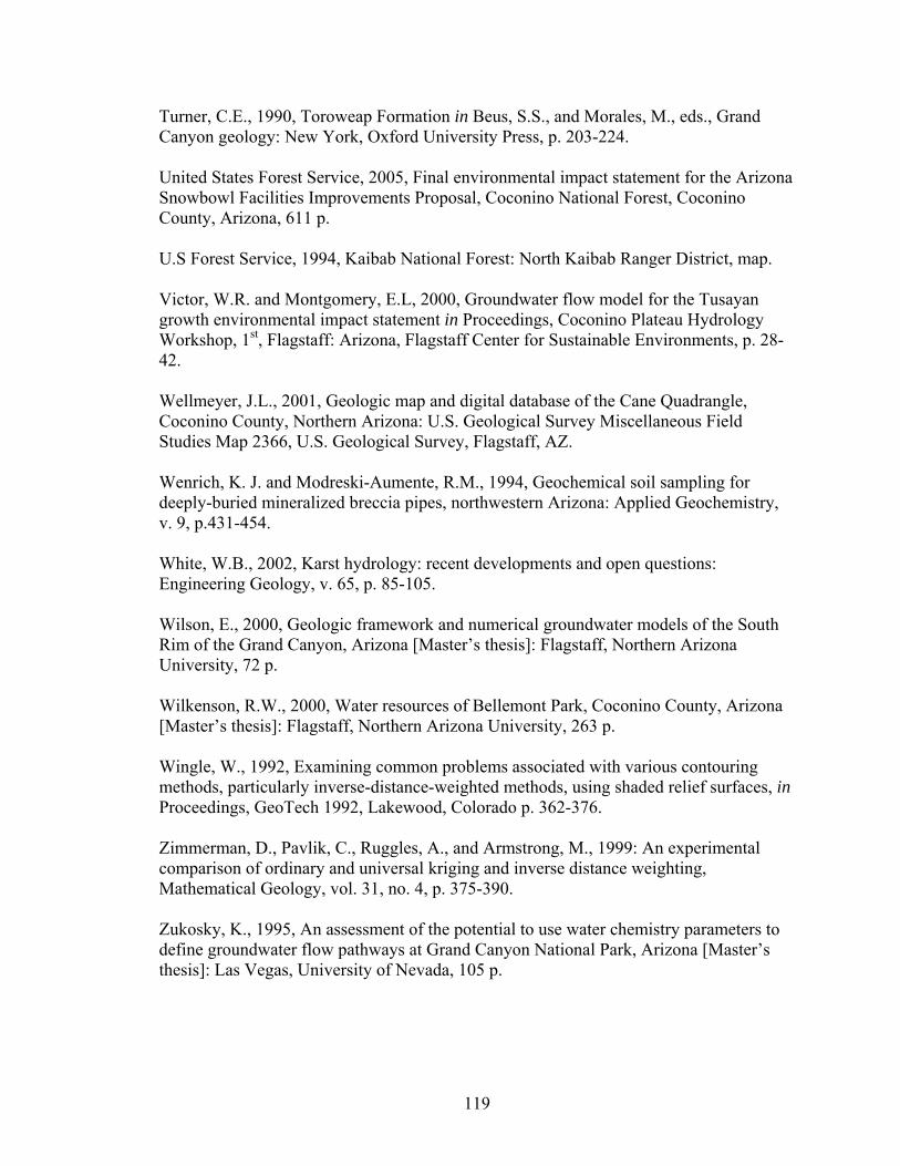
119
Turner, C.E., 1990, Toroweap Formation in Beus, S.S., and Morales, M., eds., Grand Canyon geology: New York, Oxford University Press, p. 203-224. United States Forest Service, 2005, Final environmental impact statement for the Arizona Snowbowl Facilities Improvements Proposal, Coconino National Forest, Coconino County, Arizona, 611 p. U.S Forest Service, 1994, Kaibab National Forest: North Kaibab Ranger District, map. Victor, W.R. and Montgomery, E.L, 2000, Groundwater flow model for the Tusayan growth environmental impact statement in Proceedings, Coconino Plateau Hydrology Workshop, 1st, Flagstaff: Arizona, Flagstaff Center for Sustainable Environments, p. 28-42. Wellmeyer, J.L., 2001, Geologic map and digital database of the Cane Quadrangle, Coconino County, Northern Arizona: U.S. Geological Survey Miscellaneous Field Studies Map 2366, U.S. Geological Survey, Flagstaff, AZ. Wenrich, K. J. and Modreski-Aumente, R.M., 1994, Geochemical soil sampling for deeply-buried mineralized breccia pipes, northwestern Arizona: Applied Geochemistry, v. 9, p.431-454. White, W.B., 2002, Karst hydrology: recent developments and open questions: Engineering Geology, v. 65, p. 85-105. Wilson, E., 2000, Geologic framework and numerical groundwater models of the South Rim of the Grand Canyon, Arizona [Master’s thesis]: Flagstaff, Northern Arizona University, 72 p. Wilkenson, R.W., 2000, Water resources of Bellemont Park, Coconino County, Arizona [Master’s thesis]: Flagstaff, Northern Arizona University, 263 p. Wingle, W., 1992, Examining common problems associated with various contouring methods, particularly inverse-distance-weighted methods, using shaded relief surfaces, in Proceedings, GeoTech 1992, Lakewood, Colorado p. 362-376. Zimmerman, D., Pavlik, C., Ruggles, A., and Armstrong, M., 1999: An experimental comparison of ordinary and universal kriging and inverse distance weighting, Mathematical Geology, vol. 31, no. 4, p. 375-390. Zukosky, K., 1995, An assessment of the potential to use water chemistry parameters to define groundwater flow pathways at Grand Canyon National Park, Arizona [Master’s thesis]: Las Vegas, University of Nevada, 105 p.

120
APPENDICES

APPENDIX A
DIGITAL GEOLOGIC FRAMEWORK MODEL GRID FILES (ENCLOSED CD)

APPENDIX B
ROARING SPRINGS 2003 FIELD SHEETS
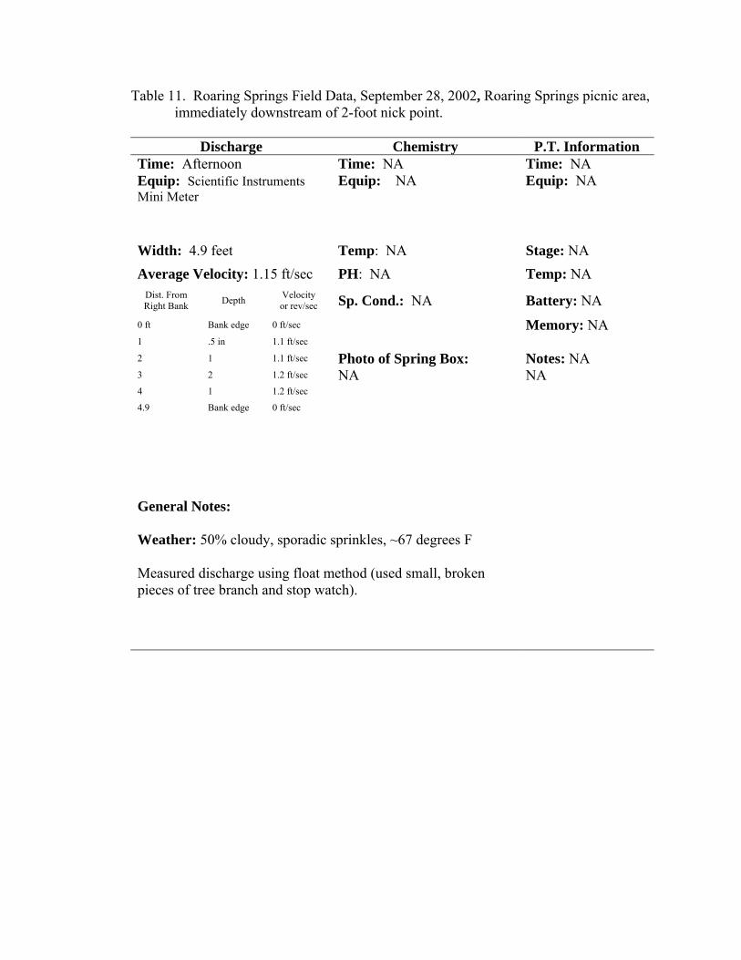
Table 11. Roaring Springs Field Data, September 28, 2002, Roaring Springs picnic area, immediately downstream of 2-foot nick point.
Discharge Chemistry P.T. Information
Time: Afternoon Time: NA Time: NA Equip: Scientific Instruments Mini Meter
Equip: NA
Equip: NA
Width: 4.9 feet Temp: NA Stage: NA Average Velocity: 1.15 ft/sec PH: NA Temp: NA
Dist. From Right Bank Depth Velocity
or rev/sec Sp. Cond.: NA Battery: NA 0 ft Bank edge 0 ft/sec Memory: NA 1 .5 in 1.1 ft/sec 2 1 1.1 ft/sec Photo of Spring Box: Notes: NA 3 2 1.2 ft/sec
4 1 1.2 ft/sec
4.9 Bank edge 0 ft/sec
NA NA
General Notes: Weather: 50% cloudy, sporadic sprinkles, ~67 degrees F Measured discharge using float method (used small, broken pieces of tree branch and stop watch).
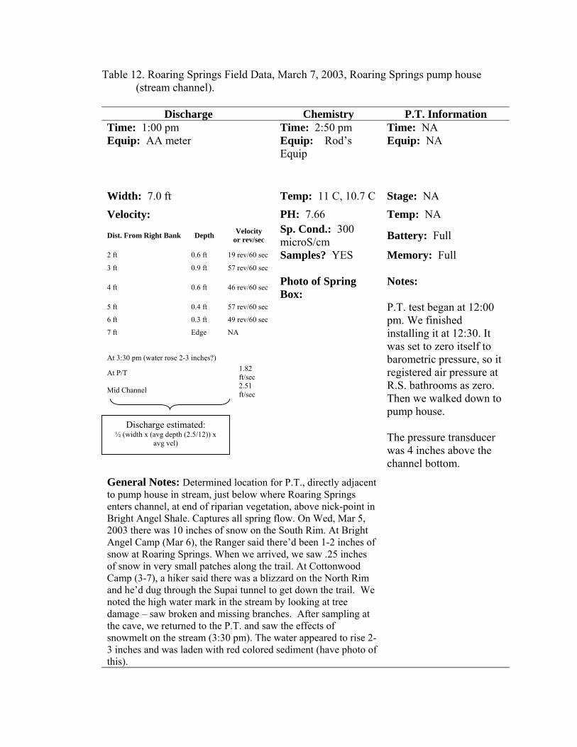
Table 12. Roaring Springs Field Data, March 7, 2003, Roaring Springs pump house (stream channel).
Discharge Chemistry P.T. Information
Time: 1:00 pm Time: 2:50 pm Time: NA Equip: AA meter
Equip: Rod’s Equip
Equip: NA
Width: 7.0 ft Temp: 11 C, 10.7 C Stage: NA Velocity: PH: 7.66 Temp: NA
Dist. From Right Bank Depth Velocity or rev/sec
Sp. Cond.: 300 microS/cm Battery: Full
2 ft 0.6 ft 19 rev/60 sec Samples? YES Memory: Full 3 ft 0.9 ft 57 rev/60 sec 4 ft 0.6 ft 46 rev/60 sec
Photo of Spring Box:
Notes:
5 ft 0.4 ft 57 rev/60 sec
6 ft 0.3 ft 49 rev/60 sec
7 ft Edge NA
At 3:30 pm (water rose 2-3 inches?)
At P/T 1.82 ft/sec
Mid Channel 2.51 ft/sec
P.T. test began at 12:00 pm. We finished installing it at 12:30. It was set to zero itself to barometric pressure, so it registered air pressure at R.S. bathrooms as zero. Then we walked down to pump house. The pressure transducer was 4 inches above the channel bottom.
General Notes: Determined location for P.T., directly adjacent to pump house in stream, just below where Roaring Springs enters channel, at end of riparian vegetation, above nick-point in Bright Angel Shale. Captures all spring flow. On Wed, Mar 5, 2003 there was 10 inches of snow on the South Rim. At Bright Angel Camp (Mar 6), the Ranger said there’d been 1-2 inches of snow at Roaring Springs. When we arrived, we saw .25 inches of snow in very small patches along the trail. At Cottonwood Camp (3-7), a hiker said there was a blizzard on the North Rim and he’d dug through the Supai tunnel to get down the trail. We noted the high water mark in the stream by looking at tree damage – saw broken and missing branches. After sampling at the cave, we returned to the P.T. and saw the effects of snowmelt on the stream (3:30 pm). The water appeared to rise 2-3 inches and was laden with red colored sediment (have photo of this).
Discharge estimated: ½ (width x (avg depth (2.5/12)) x
avg vel)
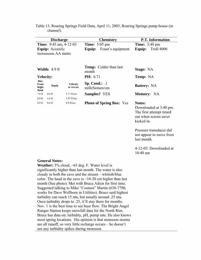
Table 13. Roaring Springs Field Data, April 11, 2003, Roaring Springs pump house (in channel).
Discharge Chemistry P.T. Information
Time: 9:45 am, 4-12-03 Time: 5:05 pm Time: 3:40 pm Equip: Scientific Instruments AA meter
Equip: Foust’s equipment
Equip: Troll 4000
Width: 8.9 ft Temp: Colder than last month Stage: NA
Velocity: PH: 6.71 Temp: NA Dist. From Right Bank
Depth Velocity or rev/sec
Sp. Cond.: .1 milleSemen/cm Battery: NA
7.6 ft 0.9 ft 1.17 ft/sec Samples? YES Memory: NA 8.0 ft 1.6 ft 1.07 ft/sec 8.9 ft 0.6 ft 8.9 ft/sec Photo of Spring Box: Yes Notes:
Downloaded at 3:40 pm. The first attempt timed out when screen saver kicked in. Pressure transducer did not appear to move from last month. 4-12-03: Downloaded at 10:40 am
General Notes: Weather: 3% cloud, ~65 deg. F. Water level is significantly higher than last month. The water is also cloudy in both the cave and the stream – whitish/blue color. The head in the cave is ~10-20 cm higher than last month (See photo). Met with Bruce Aiken for first time. Suggested talking to Mike “Cosmos” Martin (638-7790, works for Dave Wellborn in Utilities). Bruce said highest turbidity can reach 15 ntu, but usually around .25 ntu. Once turbidity drops to .25, it’ll stay there for months. Nov. 1 is the best time to see base flow. The Bright Angel Ranger Station keeps snowfall data for the North Rim. Bruce has data on: turbidity, pH, pump rate. He also knows most spring locations. His opinion is that monsoon storms are all runoff, so very little recharge occurs – he doesn’t see any turbidity spikes during monsoon.
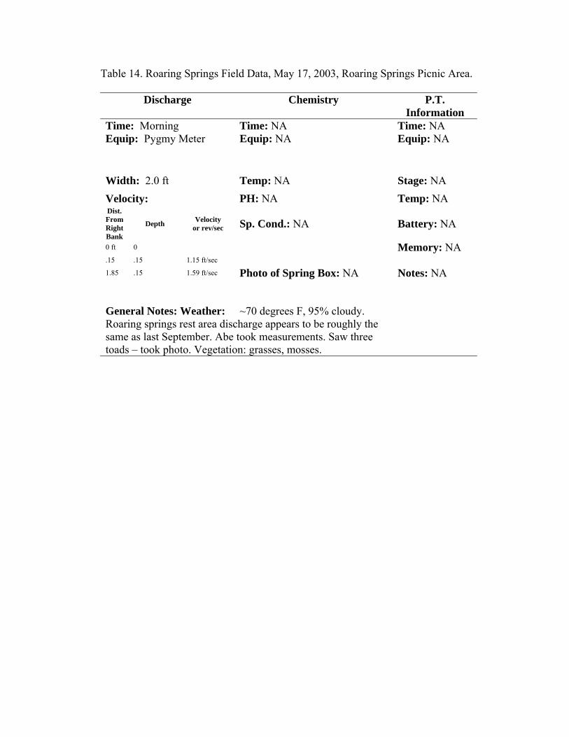
Table 14. Roaring Springs Field Data, May 17, 2003, Roaring Springs Picnic Area.
Discharge Chemistry P.T. Information
Time: Morning Time: NA Time: NA Equip: Pygmy Meter
Equip: NA
Equip: NA
Width: 2.0 ft Temp: NA Stage: NA Velocity: PH: NA Temp: NA Dist. From Right Bank
Depth Velocity or rev/sec Sp. Cond.: NA Battery: NA
0 ft 0 Memory: NA .15 .15 1.15 ft/sec 1.85 .15 1.59 ft/sec Photo of Spring Box: NA Notes: NA
General Notes: Weather: ~70 degrees F, 95% cloudy. Roaring springs rest area discharge appears to be roughly the same as last September. Abe took measurements. Saw three toads – took photo. Vegetation: grasses, mosses.
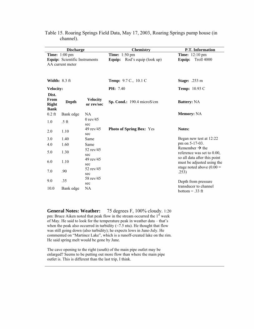
Table 15. Roaring Springs Field Data, May 17, 2003, Roaring Springs pump house (in channel).
Discharge Chemistry P.T. Information
Time: 1:00 pm Time: 1:50 pm Time: 12:10 pm Equip: Scientific Instruments AA current meter
Equip: Rod’s equip (look up)
Equip: Troll 4000
Width: 8.3 ft Temp: 9.7 C., 10.1 C Stage: .253 m
Velocity: PH: 7.40 Temp: 10.93 C Dist. From Right Bank
Depth Velocity or rev/sec Sp. Cond.: 190.4 microS/cm Battery: NA
0.2 ft Bank edge NA Memory: NA
1.0 .5 ft 0 rev/45 sec
2.0 1.10 49 rev/45 sec
Photo of Spring Box: Yes Notes:
3.0 1.40 Same 4.0 1.60 Same
5.0 1.30 52 rev/45 sec
6.0 1.10 49 rev/45 sec
7.0 .90 52 rev/45 sec
9.0 .35 58 rev/45 sec
10.0 Bank edge NA
Began new test at 12:22 pm on 5-17-03. Remember the reference was set to 0.00, so all data after this point must be adjusted using the stage noted above (0.00 = .253) Depth from pressure transducer to channel bottom = .33 ft
General Notes: Weather: 75 degrees F, 100% cloudy. 1:20 pm: Bruce Aiken noted that peak flow in the stream occurred the 1st week of May. He said to look for the temperature peak in weather data – that’s when the peak also occurred in turbidity (~7.5 ntu). He thought that flow was still going down (also turbidity); he expects lows in June-July. He commented on “Martinez Lake”, which is a runoff-created lake on the rim. He said spring melt would be gone by June. The cave opening to the right (south) of the main pipe outlet may be enlarged? Seems to be putting out more flow than where the main pipe outlet is. This is different than the last trip, I think.
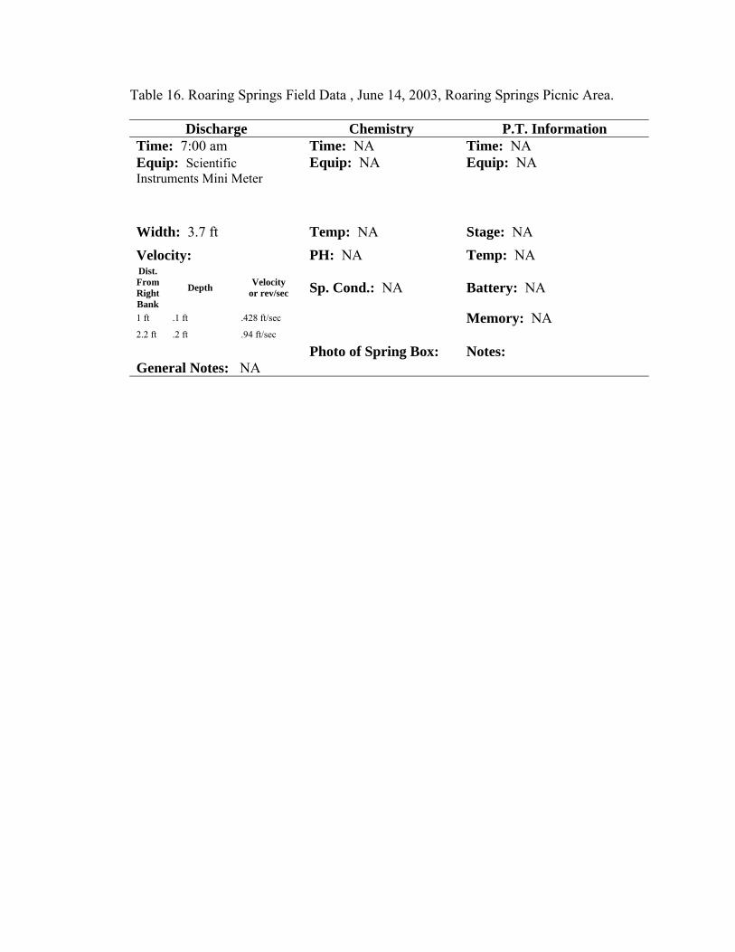
Table 16. Roaring Springs Field Data , June 14, 2003, Roaring Springs Picnic Area.
Discharge Chemistry P.T. Information Time: 7:00 am Time: NA Time: NA Equip: Scientific Instruments Mini Meter
Equip: NA
Equip: NA
Width: 3.7 ft Temp: NA Stage: NA Velocity: PH: NA Temp: NA Dist. From Right Bank
Depth Velocity or rev/sec Sp. Cond.: NA Battery: NA
1 ft .1 ft .428 ft/sec Memory: NA 2.2 ft .2 ft .94 ft/sec Photo of Spring Box: Notes: General Notes: NA
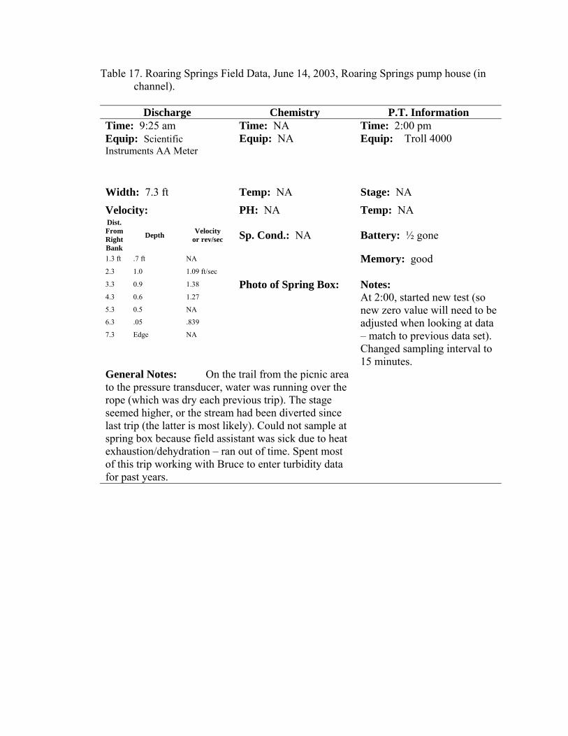
Table 17. Roaring Springs Field Data, June 14, 2003, Roaring Springs pump house (in channel).
Discharge Chemistry P.T. Information
Time: 9:25 am Time: NA Time: 2:00 pm Equip: Scientific Instruments AA Meter
Equip: NA
Equip: Troll 4000
Width: 7.3 ft Temp: NA Stage: NA Velocity: PH: NA Temp: NA Dist. From Right Bank
Depth Velocity or rev/sec Sp. Cond.: NA Battery: ½ gone
1.3 ft .7 ft NA Memory: good 2.3 1.0 1.09 ft/sec 3.3 0.9 1.38 Photo of Spring Box: Notes: 4.3 0.6 1.27
5.3 0.5 NA
6.3 .05 .839
7.3 Edge NA
At 2:00, started new test (so new zero value will need to be adjusted when looking at data – match to previous data set). Changed sampling interval to 15 minutes.
General Notes: On the trail from the picnic area to the pressure transducer, water was running over the rope (which was dry each previous trip). The stage seemed higher, or the stream had been diverted since last trip (the latter is most likely). Could not sample at spring box because field assistant was sick due to heat exhaustion/dehydration – ran out of time. Spent most of this trip working with Bruce to enter turbidity data for past years.
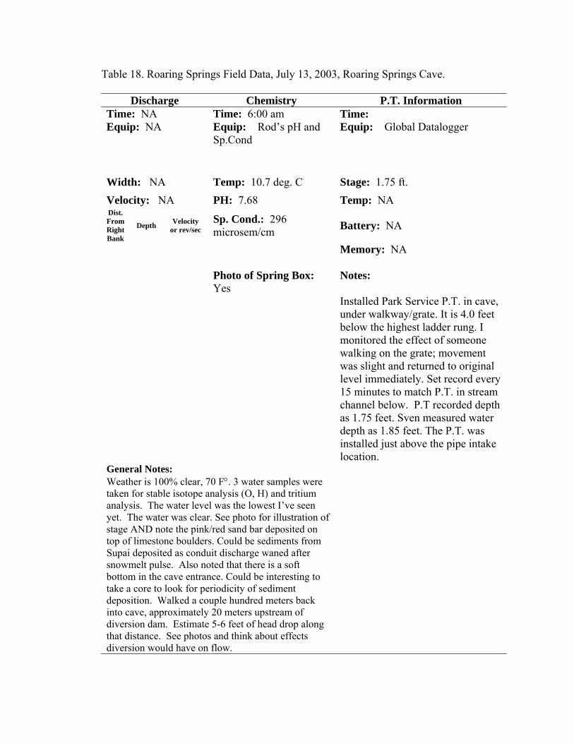
Table 18. Roaring Springs Field Data, July 13, 2003, Roaring Springs Cave.
Discharge Chemistry P.T. Information Time: NA Time: 6:00 am Time: Equip: NA
Equip: Rod’s pH and Sp.Cond
Equip: Global Datalogger
Width: NA Temp: 10.7 deg. C Stage: 1.75 ft. Velocity: NA PH: 7.68 Temp: NA Dist. From Right Bank
Depth Velocity or rev/sec
Sp. Cond.: 296 microsem/cm Battery: NA
Memory: NA
Photo of Spring Box: Yes
Notes:
Installed Park Service P.T. in cave, under walkway/grate. It is 4.0 feet below the highest ladder rung. I monitored the effect of someone walking on the grate; movement was slight and returned to original level immediately. Set record every 15 minutes to match P.T. in stream channel below. P.T recorded depth as 1.75 feet. Sven measured water depth as 1.85 feet. The P.T. was installed just above the pipe intake location.
General Notes: Weather is 100% clear, 70 F°. 3 water samples were taken for stable isotope analysis (O, H) and tritium analysis. The water level was the lowest I’ve seen yet. The water was clear. See photo for illustration of stage AND note the pink/red sand bar deposited on top of limestone boulders. Could be sediments from Supai deposited as conduit discharge waned after snowmelt pulse. Also noted that there is a soft bottom in the cave entrance. Could be interesting to take a core to look for periodicity of sediment deposition. Walked a couple hundred meters back into cave, approximately 20 meters upstream of diversion dam. Estimate 5-6 feet of head drop along that distance. See photos and think about effects diversion would have on flow.
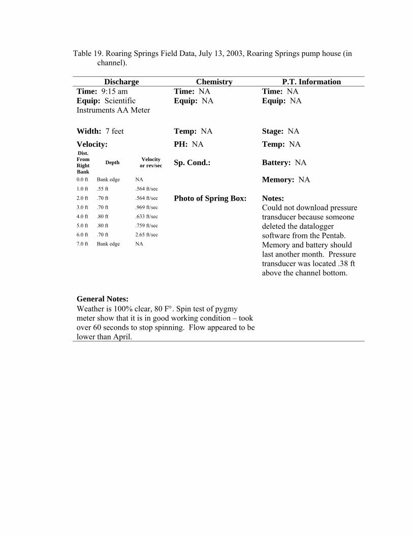
Table 19. Roaring Springs Field Data, July 13, 2003, Roaring Springs pump house (in channel).
Discharge Chemistry P.T. Information
Time: 9:15 am Time: NA Time: NA Equip: Scientific Instruments AA Meter
Equip: NA
Equip: NA
Width: 7 feet Temp: NA Stage: NA Velocity: PH: NA Temp: NA Dist. From Right Bank
Depth Velocity or rev/sec Sp. Cond.: Battery: NA
0.0 ft Bank edge NA Memory: NA 1.0 ft .55 ft .564 ft/sec 2.0 ft .70 ft .564 ft/sec Photo of Spring Box: Notes: 3.0 ft .70 ft .969 ft/sec
4.0 ft .80 ft .633 ft/sec
5.0 ft .80 ft .759 ft/sec
6.0 ft .70 ft 2.65 ft/sec
7.0 ft Bank edge NA
Could not download pressure transducer because someone deleted the datalogger software from the Pentab. Memory and battery should last another month. Pressure transducer was located .38 ft above the channel bottom.
General Notes: Weather is 100% clear, 80 F°. Spin test of pygmy meter show that it is in good working condition – took over 60 seconds to stop spinning. Flow appeared to be lower than April.
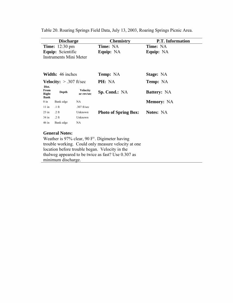
Table 20. Roaring Springs Field Data, July 13, 2003, Roaring Springs Picnic Area.
Discharge Chemistry P.T. Information Time: 12:30 pm Time: NA Time: NA Equip: Scientific Instruments Mini Meter
Equip: NA
Equip: NA
Width: 46 inches Temp: NA Stage: NA Velocity: > .307 ft/sec PH: NA Temp: NA Dist. From Right Bank
Depth Velocity or rev/sec Sp. Cond.: NA Battery: NA
0 in Bank edge NA Memory: NA 11 in .1 ft .307 ft/sec 23 in .2 ft Unknown Photo of Spring Box: Notes: NA 34 in .2 ft Unknown
46 in Bank edge NA
General Notes: Weather is 97% clear, 90 F°. Digimeter having trouble working. Could only measure velocity at one location before trouble began. Velocity in the thalweg appeared to be twice as fast? Use 0.307 as minimum discharge.
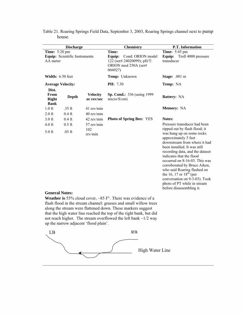
Table 21. Roaring Springs Field Data, September 3, 2003, Roaring Springs channel next to pump house.
Discharge Chemistry P.T. Information
Time: 5:20 pm Time: Time: 5:45 pm Equip: Scientific Instruments AA meter
Equip: Cond: ORION model 122 (ser# 24020099); pH/T: ORION mod 250A (ser# 004927)
Equip: Troll 4000 pressure transducer
Width: 6.50 feet Temp: Unknown Stage: .001 m
Average Velocity: PH: 7.30 Temp: NA Dist. From Right Bank
Depth Velocity or rev/sec
Sp. Cond.: 336 (using 1999 micro/S/cm) Battery: NA
1.0 ft .35 ft 41 rev/min Memory: NA 2.0 ft 0.4 ft 40 rev/min 3.0 ft 0.4 ft 42 rev/min Photo of Spring Box: YES Notes: 4.0 ft 0.5 ft 57 rev/min
5.0 ft .05 ft 102 rev/min
Pressure transducer had been ripped out by flash flood; it was hung up on some rocks approximately 5 feet downstream from where it had been installed. It was still recording data, and the dataset indicates that the flood occurred on 8-16-03. This was corroborated by Bruce Aiken, who said Roaring flashed on the 16, 17 or 18th (per conversation on 9-3-03). Took photo of PT while in stream before disassembling it.
General Notes: Weather is 55% cloud cover, ~85 F°. There was evidence of a flash flood in the stream channel: grasses and small willow trees along the stream were flattened down. These markers suggest that the high water line reached the top of the right bank, but did not reach higher. The stream overflowed the left bank ~1/2 way up the narrow adjacent ‘flood plain’.
RBLB
High Water Line
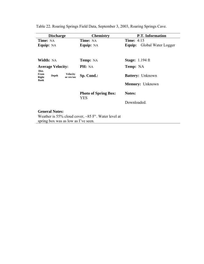
Table 22. Roaring Springs Field Data, September 3, 2003, Roaring Springs Cave.
Discharge Chemistry P.T. Information Time: NA Time: NA Time: 4:15 Equip: NA
Equip: NA
Equip: Global Water Logger
Width: NA Temp: NA Stage: 1.194 ft Average Velocity: PH: NA Temp: NA Dist. From Right Bank
Depth Velocity or rev/sec Sp. Cond.: Battery: Unknown
Memory: Unknown
Photo of Spring Box: YES
Notes:
Downloaded.
General Notes: Weather is 55% cloud cover, ~85 F°. Water level at spring box was as low as I’ve seen.
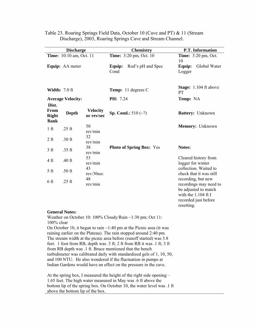
Table 23. Roaring Springs Field Data, October 10 (Cave and PT) & 11 (Stream Discharge), 2003, Roaring Springs Cave and Stream Channel.
Discharge Chemistry P.T. Information
Time: 10:10 am, Oct. 11 Time: 3:20 pm, Oct. 10 Time: 3:20 pm, Oct. 10
Equip: AA meter
Equip: Rod’s pH and Spec Cond
Equip: Global Water Logger
Width: 7.0 ft Temp: 11 degrees C Stage: 1.104 ft above PT
Average Velocity: PH: 7.24 Temp: NA Dist. From Right Bank
Depth Velocity or rev/sec Sp. Cond.: 510 (~?) Battery: Unknown
1 ft .25 ft 50 rev/min
Memory: Unknown
2 ft .30 ft 32 rev/min
3 ft .35 ft 38 rev/min
Photo of Spring Box: Yes Notes:
4 ft .40 ft 53 rev/min
5 ft .50 ft 43 rev/30sec
6 ft .25 ft 48 rev/min
Cleared history from logger for winter collection. Waited to check that it was still recording, but new recordings may need to be adjusted to match with the 1.104 ft I recorded just before resetting.
General Notes: Weather on October 10: 100% Cloudy/Rain ~1:30 pm; Oct 11: 100% clear On October 10, it began to rain ~1:40 pm at the Picnic area (it was raining earlier on the Plateau). The rain stopped around 2:40 pm. The stream width at the picnic area before (runoff started) was 3.8 feet. 1 foot from RB, depth was .3 ft; 2 ft from RB it was .1 ft; 3 ft from RB depth was .1 ft. Bruce mentioned that the bench turbidimeter was calibrated daily with standardized gels of 1, 10, 50, and 100 NTU. He also wondered if the fluctuation in pumps at Indian Gardens would have an effect on the pressure in the cave. At the spring box, I measured the height of the right side opening – 1.65 feet. The high water measured in May was .6 ft above the bottom lip of the spring box. On October 10, the water level was .1 ft above the bottom lip of the box.

APPENDIX C
ROARING SPRINGS 2003 HYDROLOGIC DATA

APPENDIX D
ROARING SPRINGS MODFLOW FILES
(ENCLOSED CD)