Embed Size (px)
Citation preview

i
INTERPRETING THE SPATIAL DISTRIBUTION OF SELECT SOIL PROPERTIES
IN TWONEW BRUNSWICK UPLAND WATERSHEDS BY WAY OF THE FLOW ACCUMULATION CONCEPT
by
Bradley S. Case
BSc.F, University of New Brunswick, 1996
A Thesis Submitted in Partial Fulfilment of the Requirements for the Degree of
Master of Science in Forestry
in the Graduate Academic Unit of Forestry
This thesis is accepted.
------------------------------------------ Dean of Graduate Studies
THE UNIVERSITY OF NEW BRUNSWICK
December, 2000
© Bradley S. Case, 2000
ii ii
ABSTRACT
This thesis investigates functional interrelationships among lateral water flow and accumulation, soil chemistry and soil physical characteristics at two contrasting upland watershed project areas near Gounamitz and Island Lakes in Northern New Brunswick. Soils and substrates are well drained at the Gounamitz Lake site, while soils at the Island Lake site suffer from restricted permeability at a half metre depth. Flow accumulation, wetness index and slope gradient values, as topographic metrics of lateral subsurface water flow, were estimated for 38 and 41 plot locations at the Gounamitz Lake and Island Lake sites respectively. Guided by both plot-level observations (landscape position, flow regime, slope shape) and digitally- modelled flow networks, I derived a set of best-estimate values for flow accumulation at each plot. Wetness index was calculated as a function of both field-estimated slope gradient and flow accumulation.
Spatial differences in depth, % coarse fragment content and % clay of A, B and subsoil layers, as well as overall soil layer and rooting zone depth, were found to be weakly related to topographic metrics. Soil chemical concentrations within these same layers, however, displayed stronger relationships overall with water flow indices. In general, trends were found to be consistent between sites, but the strength of these correlations differed. Total elemental nutrient amounts per hectare of rooting zone were also influenced by topography, soil acidity and soil clay content; relationships were both linear and non-linear and varied by nutrient element and site. Overall, the basic differences in substrate permeability between sites has likely regulated the amount of lateral versus downward water percolation, thereby influencing the resultant ridge-to-depression pattern of soil accumulated nutrients and particulate matter. In general, basins with poor soil permeability show a stronger ridge-to-depression spatial accumulation pattern than basins with well-drained soils and substrates. Also investigated were two field procedures to obtain accurate elevation data. Within a portion of the Island Lake site, point positions and elevations were surveyed using manual (chain and compass) and hybrid manual/GPS methods and geo-referenced using a number of known control points. Digital Elevation Models created from these data (10 – 20 m grid resolution) were visibly more capable of resolving finer scale landform features as compared to provincial data sets (70 m grid resolution).
iii iii
TABLE OF CONTENTS
CHAPTER 1. THESIS INTRODUCTION ...................................................... 1
CHAPTER 2. THE PROJECT SITES – SITE AND PLOT DESCRIPTIONS
AND FIELD METHODOLOGIES ....................................................... 5
INTRODUCTION ................................................................................................ 5
SITE SELECTION RATIONALE ........................................................................ 5
GENERAL PROJECT SITE DESCRIPTIONS ................................................... 8
Island Lake Site ............................................................................................ 8
Gounamitz Lake Site ................................................................................... 9
PLOT SELECTION, ESTABLISHMENT AND SAMPLING ......................... 9
PLOT-LEVEL CHARACTERISTICS ............................................................. 12
Island Lake Site ........................................................................................... 12
Gounamitz Lake Site .................................................................................. 14
CHAPTER 3. DERIVING WATER FLOW AND ACCUMULATION
ATTRIBUTES: A CONSIDERATION OF SCALE AND
TOPOGRAPHIC COMPLEXITY .......................................................... 16
INTRODUCTION ................................................................................................ 16
FLOW ACCUMULATION AND WETNESS INDEX AS HYDROLOGIC
INDICES .................................................................................................... 17
METHODS ............................................................................................................. 19
Deriving Topographic Attribute Values from Available DEM Data ... 19
Deriving Expected Values as a Best Estimate ........................................ 21
RESULTS AND DISCUSSION ........................................................................... 24
Evaluation of DEM-derived Attributes and the Influence of
DEM Scale ................................................................................................... 24
Estimated Values ........................................................................................ 28
SUMMARY ........................................................................................................... 32
iv iv
CHAPTER 4. THE INFLUENCE OF TOPOGRAPHY ON SOIL PHYSICAL
PROPERTY DISTRIBUTION ................................................................ 33
INTRODUCTION ............................................................................................... 33
BACKGROUND .................................................................................................. 34
METHODS ........................................................................................................... 39
Description of Sites, Sample Plots, and Field Methodologies ............ 39
Laboratory and Statistical Methods ....................................................... 39
RESULTS AND DISCUSSION .......................................................................... 40
Soil Texture Analysis ................................................................................ 40
Overall Physical Property Variability ..................................................... 42
Thickness of Soil Layers and Rooting Zone ........................................... 44
Forest Floor Thickness ..................................................................... 44
A Layer Thickness ............................................................................ 47
B Layer Thickness ............................................................................. 47
Effective Rooting Depth and Subsoil Thickness .......................... 48
% Coarse Fragments .................................................................................. 50
% Clay .......................................................................................................... 52
SUMMARY .......................................................................................................... 54
CHAPTER 5. THE INFLUENCE OF WATER FLOW AND
ACCUMULATION AND PARENT MATERIAL ON SOIL
CHEMICAL DISTRIBUTIONS ......................................................... 56
INTRODUCTION ................................................................................................ 56
METHODS ............................................................................................................ 58
Description of Sites, Sample Plots, and Field Methodologies ............. 58
Soil Sample Preparation and Laboratory Analysis ............................... 58
Topographic and Statistical Analyses ..................................................... 59
RESULTS AND DISCUSSION ........................................................................... 60
Soil Variability............................................................................................ 60
Influence of Flow Accumulation on Soil Chemistry ............................. 62
v v
The Added Influence of Parent Material ................................................ 67
SUMMARY ........................................................................................................... 72
CHAPTER 6. ROOTING ZONE NUTRIENT POOLS AT THE ISLAND
LAKE AND GOUNAMITZ LAKE SITES: THE INFLUENCE OF
SITE AND TOPOGRAPHY ................................................................... 76
INTRODUCTION ................................................................................................ 76
METHODS ............................................................................................................ 76
RESULTS AND DISCUSSION ........................................................................... 78
Overall Distribution and Trends ............................................................. 78
Total Carbon and Nitrogen ............................................................. 81
Phosphorous ..................................................................................... 83
Potassium, Calcium, and Magnesium ........................................... 84
The Influence of Water Flow and Accumulation .................................. 85
Total Carbon and Nitrogen ............................................................. 86
Phosphorous ..................................................................................... 90
Potassium, Calcium, and Magnesium ........................................... 92
SUMMARY ........................................................................................................... 97
CHAPTER 7. TWO SURVEY METHODS FOR CREATING FINE-SCALE
DEM’S UNDER A FOREST CANOPY: A QUALITATIVE
ANALYSIS ............................................................................................... 100
INTRODUCTION ................................................................................................ 100
METHODS ............................................................................................................ 101
Two Field Survey Methods for Creating a Fine-scale DEM.................. 101
Polychain Method ............................................................................. 101
Hybrid Manual/GPS Method ........................................................ 102
Organisation and Analysis of Survey Data ............................................ 105
RESULTS AND DISCUSSION ........................................................................... 107
Polychain Method ...................................................................................... 107
Hybrid Manual/GPS Method .................................................................. 107
vi vi
Identifying Sources of Error: A Caveat .................................................. 110
SUMMARY AND RECOMMENDATIONS ..................................................... 112
CHAPTER 8. THESIS CONCLUSION .......................................................... 114
SYNTHESIS .......................................................................................................... 114
OVERALL CONTRIBUTIONS .......................................................................... 119
LITERATURE CITED ........................................................................................ 122
APPENDIX 1. NUTRIENT CORRELATION TABLES ............................... 132
LIST OF TABLES
Table 2.1. Summary of site and soil characteristics for plots within the Island Lake
sub-catchments. ..............................................…………….. 13
Table 2.2. Summary of site and soil characteristics for plots within the Gounamitz
Lake sub-catchments. ......................................…………………. 15
Table 3.1. A comparison of expected and DEM-derived topographic attribute
values for plot locations at the Island Lake site. ...............…… 25
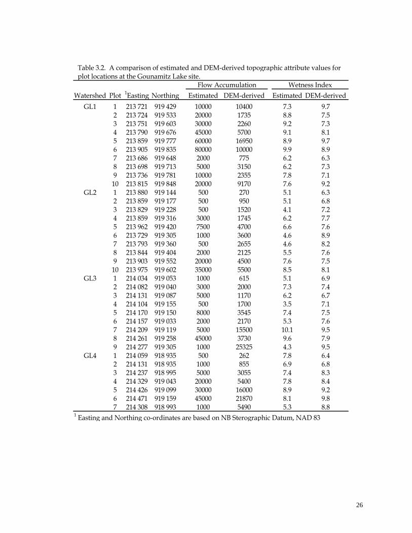
Table 3.2. A comparison of expected and DEM-derived topographic attribute
values for plot locations at the Gounamitz Lake site. ....……. 26
Table 4.1. A representative literature summary of typical meso-scale (5-100ha)
investigations concerning the variability and spatial distribution of soil
physical properties and the influence of topography. .…….. 35
Table 4.2. Cross-tabulation of outcomes for the feel test and hydrometer methods
of texture determination for a) Island Lake and b) Gounamitz Lake
sites. .……………………………………………………………… 41
Table 4.3. Summary statistics of averaged physical property data for the forest floor
(FF), A, B, and subsoil (SS) layers at the Island Lake and Gounamitz Lake
study sites. ...................……………………… 43
Table 5.1. Summary statistics of averaged chemical data for the forest floor
(FF), A, B, and subsoil (SS) layers at the Island Lake and Gounamitz Lake
study sites. ............................................................………… 61
vii vii
Table 5.2. Coefficients of determination for simple linear regressions between flow
accumulation and soil chemical concentrations by soil layer
and project site (p<0.05). .........................................................…. . 64
Table 5.3. Multiple regression equations (p<0.10) relating topographic/site
variables to soil chemistry in mineral soil layers at the Island Lake
site. R2 values for simple regressions with flow accumulation alone
(from Table 5.2) are shown for comparison. .........................…. 68
Table 5.4. Multiple regression equations (p<0.10) relating topographic/site
variables to soil chemistry in mineral soil layers at the Gounamitz Lake
site. R2 values for simple regressions with flow accumulation alone (from
Table 5.2) are shown for comparison. ......……………… 69
Table 6.1. Descriptive statistics for rooting zone totals of carbon and major
nutrients at the two study sites. ...............................................… 80
LIST OF FIGURES
Figure 2.1. Location of study sites within the Province of New
Brunswick ………………………………………………………... 6
Figure 2.2. Plot locations within the a) Island Lake and b) Gounamitz Lake
sub-catchments. Both plots and sub-catchments are
numbered. ....................................................................................… 10
Figure 3.1. Flow networks generated using the DEMON algorithm for the a) Island
Lake and b) Gounamitz Lake project sites draped over
15m interpolated DEM’s. Black dots represent sample
points. …………………………………………………………..… 20
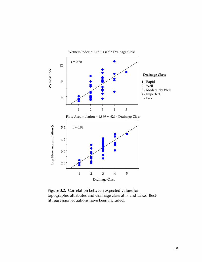
Figure 3.2. Correlation between expected values for topographic attributes
and drainage class at Island Lake. Best-fit equations have been
included. ...................................................................................….. 30
Figure 3.3. Box-plot diagrams showing variation in topographic attributes in
relation to soil class at the Gounamitz Lake site. .................…. 31
viii viii
Figure 4.1. Best-fit regressions relating layer thickness (cm) and topographic
attributes for the a) forest floor, b) A, c) B, and d) subsoil layers
at the Island Lake site. ........................................................…….. 45
Figure 4.2. Best-fit regressions relating layer thickness (cm) and topographic
attributes for the a) forest floor, b) A, c) B, and d) subsoil layers at the
Gounamitz Lake site. .........................................................…….. 46
Figure 4.3. Best-fit regressions relating rooting depth (cm) and topographic
attributes for the a) Island Lake and b) Gounamitz Lake
sites. ...........................................................................................…. 49
Figure 4.4. Best-fit regressions relating % coarse fragments and topographic
attributes at the Island Lake site for the mineral soil layers. ... 51
Figure 4.5. Best-fit regressions relating % clay and topographic attributes at
the a) Island Lake and b) Gounamitz Lake sites for the B and subsoil
layers. Bracketed points were removed from the analysis. ... 53
Figure 5.1. Relationships between flow accumulation and select soil chemical
concentrations by watershed and soil horizon. Refer to Table 5.2 for
regression statistics. ................................................................….. 63
Figure 6.1. Mean values for bulk density across soil layers at the two study
sites. ...........................................................................................….. 79
Figure 6.2. Trends in mean values (+1 S.E.) for carbon and nutrient quantities
across soil layers for both study sites. .................................….. 82
Figure 6.3. Scatter plots showing trends between Total C pools (kg/ha) and % Clay
and subsoil pH for the a) Island Lake and b) Gounamitz Lake sites,
respectively. ........................................................………… 87
Figure 6.4. Best-fit relationships between Total N pools (kg/ha) and
topographic and soil variables for the a) Island Lake and b)
Gounamitz Lake sites. .................……………………………… 89
Figure 6.5. Relationships between available P pools (kg/ha) and
ix ix
topographic and soil variables for the a) Island Lake and b) Gounamitz
Lake sites. ………………………………………….. 91
Figure 6.6. Scatter plot showing trend between K pools (kg/ha) and Subsoil pH for
the Island Lake site. Dotted line indicates evident groupings of values
based on pH. Bracketed outlier was removed from
regression. ……………………………………………………..... . 93
Figure 6.7. Best-fit relationships between available a) Ca and b) Mg pools (kg/ha)
and topographic and soil variables for the Island Lake site. .. 94
Figure 6.8. Scatter plots showing trends between available a) Ca and
b) Mg pools (kg/ha) and A Layer pH for the Gounmitz Lake site.
Cation values show obvious grouping as indicated by dotted lines.
Bracketed outliers were omitted from regressions. ………….. 95
Figure 6.9. Best-fit relationship between available K pools (kg/ha) and topographic
and soil variables for the Gounamitz Lake site. .. 96
Figure 7.1. Distributions of elevation sample points obtained from a)
Polychain and GPS survey methods and b) the Province of New
Brunswick. ................................................................................….. 106
Figure 7.2. A comparison of DEM’s created with a) data collected using the
Polychain method and b) New Brunswick provincial elevation data for
the lower portion of the IL 1 sub-catchment. ...............……. 108
Figure 7.3. A comparison of DEM’s created with a) data collected using the
polychain/GPS methods and b) NB elevation data for the IL 1 and 2
sub-catchments. ...........................................................................… 109
Figure 8.1. Diagrammatic representation of hypothesised hydro-geologic
conditions occurring at the Island Lake site. At this hummocky site,
water flows laterally along subsurface soil layers from divergent to
convergent areas. Overland flow conditions may also occur at peak
flow events as hollows fill with water. ....................................… 117

x x
Figure 8.2 Diagrammatic representation of hypothesised hydro-geologic
conditions occurring at the Gounamitz Lake site. Vertical water flow
through the soil parent material and fractured bedrock outweighs
surface and subsurface flow at this rolling site. ………………. 118
1
CHAPTER 1
THESIS INTRODUCTION
Water flow and accumulation have been recognised as mediating influences
on soil development processes in many landscapes (Jenny 1980; Gerrard 1981;
Moore et al. 1993), especially where the soil substrate becomes relatively
impermeable with depth, resulting in lateral surface and subsurface water flow and
variable soil moisture conditions (O’Loughlin 1986). The influence of water has
been succinctly summarised by Hammer (1998): “Water shapes the landscape,
participates in chemical and physical weathering, carries dissolved and suspended
materials to different places in the soil profile, landscape, or drainage network, and
is the solution within which new compounds are formed from the products of
weathering.”
Previous investigations have exhibited three main limitations in addressing
the influence of water flow and accumulation on soil development. First of all,
either directly or indirectly, studies have often lacked a consistent quantitative
framework (Pennock et al. 1987; Moore et al. 1993). For example, the use of
qualitative topographic descriptors such as slope position is subjective, may not link
directly to the effect of water flow, and does not provide a quantitative means of
duplication in other areas. Secondly, many studies have lacked the clear spatial
contrasts necessary for understanding the form and function of soil-landscape
2 2
relationships. Finally, many ecologists and soil researchers have limited their
investigations to two-dimensional soil processes or those occurring in the surface
soil (Hammer 1998), providing only a partial picture of actual soil development.
The following thesis aims to provide both a logical framework and a quantitative
methodology by which to address these shortcomings.
Two geomorphologically-contrasting headwater catchment areas in
Northern New Brunswick are characterised (Chapter 2). For a given climate and
geomorphology, watersheds become the natural unit of integration for soil
processes (Hugget, 1975; Gerrard 1981) since (1) they provide discrete, bounded
units where the flow of energy, water and chemicals can be quantified, as
determined by the local topography and (2) they occur as repeating units across a
given landscape, easily outlined with current GIS techniques. Within this
framework, relationships between lateral water flow and accumulation indices and
spatial patterns of soil properties within the rooting zone are investigated.
A main consideration, although rarely addressed, is the ability to accurately
quantify or index water flow across the landscape. Digital Elevation Models
(DEM’s) provide a means of automatically deriving quantitative topographic
attributes (see Moore et al. 1991) as quantitative indices of water flow processes.
However, the accuracy of derived attributes is directly dependent on the resolution
of the original elevation data and their usefulness in accurately characterising a
landscape at the scale desired (Zhang and Montgomery 1994). I therefore examine
the accuracy and adequacy of readily available DEM data in characterising the
3 3
topography of these two areas, as well as in deriving topographic attributes for
sample plots (Chapter 3). As an alternative to the above, automated approach, I
assign a set of a priori “best-estimate” values to each plot using field observations
and watershed flow networks, and compare them with DEM-derived values.
The quantitative topographic indices flow accumulation, slope gradient and
steady-state wetness index are hydrologically-significant spatial indicators of water
flow and accumulation mechanisms (Speight 1974; O’Loughlin 1986; Moore et al.
1991). These indices may provide a means to quantify the extent and direction of
relationships between topography and soil properties; this quantitative approach is
necessary to better understand the underlying mechanisms driving functional
relationships. Walker et al. (1968) and Moore (1996) respectively found slope
gradient and wetness index to be significant quantitative predictors of various soil
properties; flow accumulation, however, has rarely been used in this way.
Using regression analyses, I explore spatial relationships between these
indices and soil physical properties (Chapter 4) and soil chemical concentrations
(Chapter 5) by soil layer across both sites. Subsequently, I examine whether similar
relationships exist for rooting zone nutrient storage (Chapter 6) since the complete
soil profile provides a more ecologically-significant indicator of site quality and
sustainable productivity. Ultimately the objective of these investigations is to
provide a more complete understanding of the potential significance of water flow
and accumulation at two watershed sites in the context of topographic complexity,
substrate and geology.

4 4
Since the resolution of available elevation data is quite often inadequate for
fine-scale studies (Dikau 1989), I subsequently explore two field procedures
(Chapter 7) for obtaining fine-scale elevation data often necessary for characterising
local topographic complexity. These practical methods are suggested as a viable
alternative to other automatic procedures for creating such data, including high
precision GPS and digital photogrammetry. DEM’s created for a portion of one
study area using the two methods are qualitatively compared to DEM’s derived
from provincial elevation data for the same area.
5 5
CHAPTER 2
THE PROJECT SITES – SITE AND PLOT DESCRIPTIONS
AND FIELD METHODOLOGIES
INTRODUCTION
This chapter provides a general overview of two experimental sites, the
Island Lake and Gounamitz Lake project areas, their selection, the establishment of
sample plots and field methodologies. Specifically, the objectives are to:
1. Outline the overall rationale for the selection of project sites,
2. Describe the general conditions at each site in terms of climate, vegetation, soils,
and topography,
3. Outline sample-plot selection and establishment procedures, and
4. Describe plot-level site characteristics.
SITE SELECTION RATIONALE
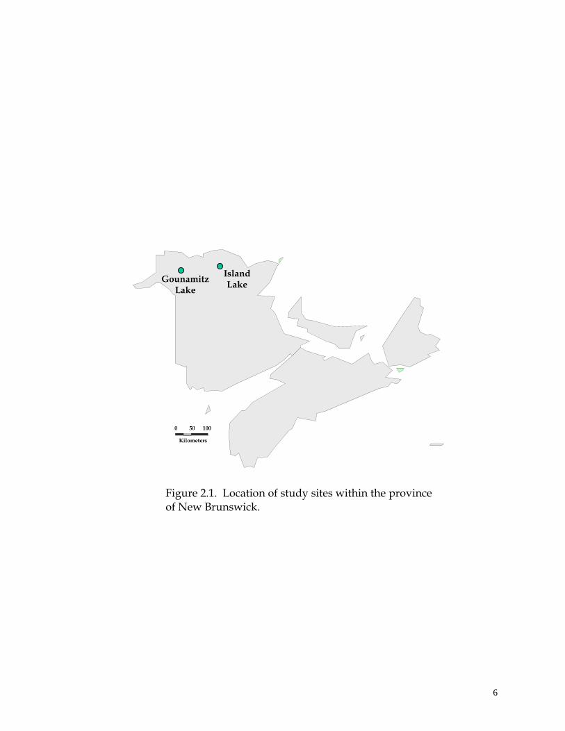
Two headwater watershed sites were selected on industrial crown-licenses
in north-central (Island Lake) and north-western (Gounamitz Lake) New Brunswick
(Figure 2.1), such that: (1) bedrock geology, surficial geology, forest cover type,
topography, and climatic conditions were different between sites, as representative
of two contrasting landscapes; and (2) the above characteristics were relatively
consistent within each site. Since this thesis deals primarily with
6 6
Gounamitz Lake
Island Lake
Figure 2.1. Location of study sites within the province of New Brunswick.
0 50
Kilometers
100
7 7
the influence of water flow and accumulation on measured biophysical site
variables, sites were chosen to isolate differing biogeochemical and hydrological
conditions, ultimately providing a study comparison between two independent
landscape types. The chosen sites are in headwater areas where perennial streams
are absent; the main hydrological influences on soil properties thus reflect surface
and subsurface water flow occurring in these areas during periods of snowmelt and
high precipitation conditions. Additionally, the two areas were selected within
relatively undisturbed, mature forestland, within the context of normal historical
forest practices.
The degree of overland and subsurface flow in a forested watershed
depends on a number of factors including the permeability and depth of soil and
parent material, the complexity and relief of topography, and the amount and
frequency of precipitation (Gerrard 1981). O’Loughlin (1986) suggested that,
because most forest soils generally are less permeable with depth, lateral water flow
is expected to occur in both a down-slope direction and toward convergent
topographic zones. At Island Lake and Gounamitz Lake sites, as is characteristic of
glacial till, soil bulk density and the percentage of coarse fragments increased with
depth causing a relative decrease in permeability; this was more characteristic of the
Island Lake site where compact, cemented or clay-enriched subsurface layers were
encountered. Further, the amount of storm-related surface and subsurface runoff is
related to the overall temporal and spatial wetness conditions (Gerrard 1981;
O’Loughlin 1986) and, thus, the water storage capacity (Burt and Butcher 1985)
8 8
prevalent in an area. Numerous depressional areas, some of them water-logged in
mid-summer, were evident at Island Lake; the rolling topography, gentle slopes
and well to rapid drainage class at Gounamitz, however, suggested that the surface
storage capacity of this area may be much lower. Initial examination suggested that
these two sites would provide an interesting contrast of the effects of water flow in
relation to substrate permeability and topographic complexity.
GENERAL PROJECT SITE DESCRIPTIONS
Island Lake Site
The Island Lake site, in the Upsalquitch site region, occurs fully within the
Popple Depot Forest Soil Unit (Colpitts et al. 1995), characterised by a compact, fine
to medium-textured glacial till of felsic volcanic and mixed igneous origin. The
topography of the area is complex, consisting of hummocky terrain with many
localised depressional areas that, upon field reconnaissance, appears to correspond
closely to the configuration of the underlying basal till and igneous bedrock. The
vegetation is principally mature black and red spruce and balsam fir, although pine
and cedar can be found on ridge and low-lying sites, respectively. Additionally
there is a component of trembling aspen and balsam poplar which grew as pioneer
species after clear-cutting 60-70 years previous and are found mostly in gently
sloping or low-lying areas.

9 9
Gounamitz Lake Site
The Gounamitz Lake site, in the Restigouche site region, falls within the
Thibault Forest Soil Unit (Colpitts et al. 1995) and is characterised by a topography
of gently rolling relief underlain by a medium-textured glacial till comprised of non
to mildly-calcareous silt-stones and shales with a high coarse fragment content.
Vegetation at this site is almost exclusively mature tolerant hardwood (yellow
birch, sugar maple, and American beech), occurring along ridges and slopes, with
white spruce and balsam fir occurring at toe-slope positions where groundwater
seepage occurs. Partial cutting, removing 30% of the hardwood overstory, had been
carried out in a portion of the site 3-4 years previous. The area experiences cool,
wet summers and cold winters with deep snow (Zelazny et al. 1989).
PLOT SELECTION, ESTABLISHMENT AND SAMPLING
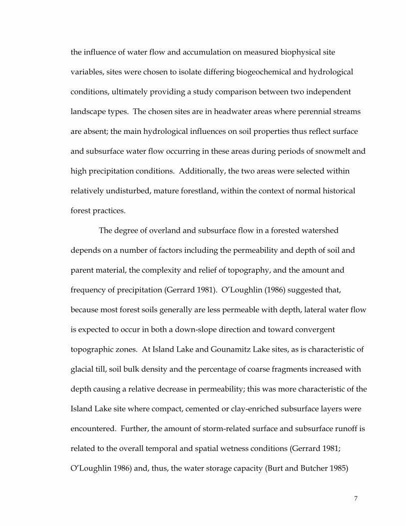
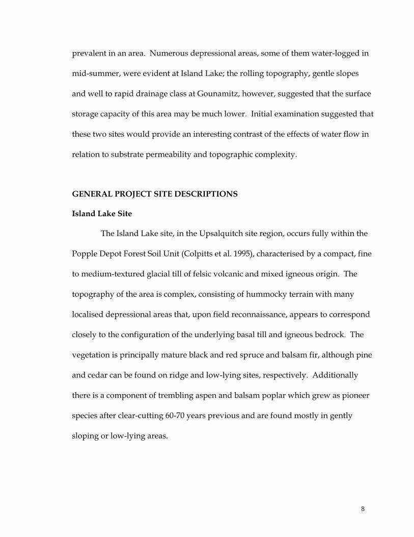
Four contiguous headwater catchments were identified within the
Gounamitz Lake (Fig. 2.2a) and Island Lake (Fig. 2.2b) project sites. A combination
of 1:50 000 topographic contour maps, aerial photo-interpretation and ground-
truthing were used to locate sub-catchment divides. Once located and flagged, the
sub-catchment boundaries were traversed with high-resolution GPS units. The
sub-catchments provided a meaningful context for identifying local drainage
networks, lateral flow conditions, and potential sample sites within each project
site.
10 10
Figure 2.2. Plot locations within the a) Island Lake and b) Gounamitz Lake sub-catchments. Both plots and sub-catchments are numbered.
6 7
5
9 8
1 2 3 4
3 7 6
4 5
1 2
10 9
6
5 8
1 2
3
10
7 4
5 9 5
4
1
2
3
6
8 7
Kilometer
s
0 0.25 0.5
1 2
4 5
3
17
16 15 18
7 8
6
2 1 3 6
4 5
1
3 2
4
9
5
9 2
7 8 9 10
12
3 4 5
6 8
1
11 13 14
7
0 0.25
Kilometer
s
0.5
IL 3
IL 4
IL 1
IL 2
GL 1
GL 2
GL 3
GL 4
N
N
a)
b)
11 11
In July/August 1997, a total of 38 and 41 sample plots were located on the
Gounamitz Lake and Island Lake sites, respectively (Figures 2.2a and b). Given
time and budget limitations, 10 plots, on average, were located per sub-catchment,
with the aim of representing both convergent flow-channel/flow-accumulation
zones and divergent flow positions. More importantly, the aim was to achieve a
sampling of perceived flow situations across the Gounamitz Lake and Island Lake
project sites that were representative of the larger area. Each plot, once located, was
geographically positioned with GPS to within a +/- 3 m accuracy.
Circular, 50 m2 sample plots (3.99 m radius) were established at each point.
One soil pit was dug at each plot down to either the C-horizon or to an
impermeable layer. A full soil profile taxonomical description was carried out
based on the Canadian Soil Classification System (Soil Classification Working
Group 1998); organic and mineral soil horizon classifications identified in the field
were later verified more accurately based on chemical data from these horizons.
Further, horizons were characterised by thickness, texture class, structure,
consistency, % coarse fragment content, degree of mottling, and root distribution
using standard procedures. A representative sample of soil was taken from each
horizon for chemical and physical analysis.
Local slope (%) and aspect were measured at each plot using a clinometer
and compass respectively. A ground vegetation and forest shrub survey was
carried out for a 30 m-radius circular area around each plot. Soil type, vegetation
type, and treatment unit designations, as indicators of relative site quality, were
12 12
determined for each plot using Forest Site Classification procedures developed for
the province of New Brunswick (Zelazny et al. 1989). Drainage class was estimated
using a standard drainage key (Jones et al. 1983).
PLOT-LEVEL CHARACTERISTICS
Island Lake Site
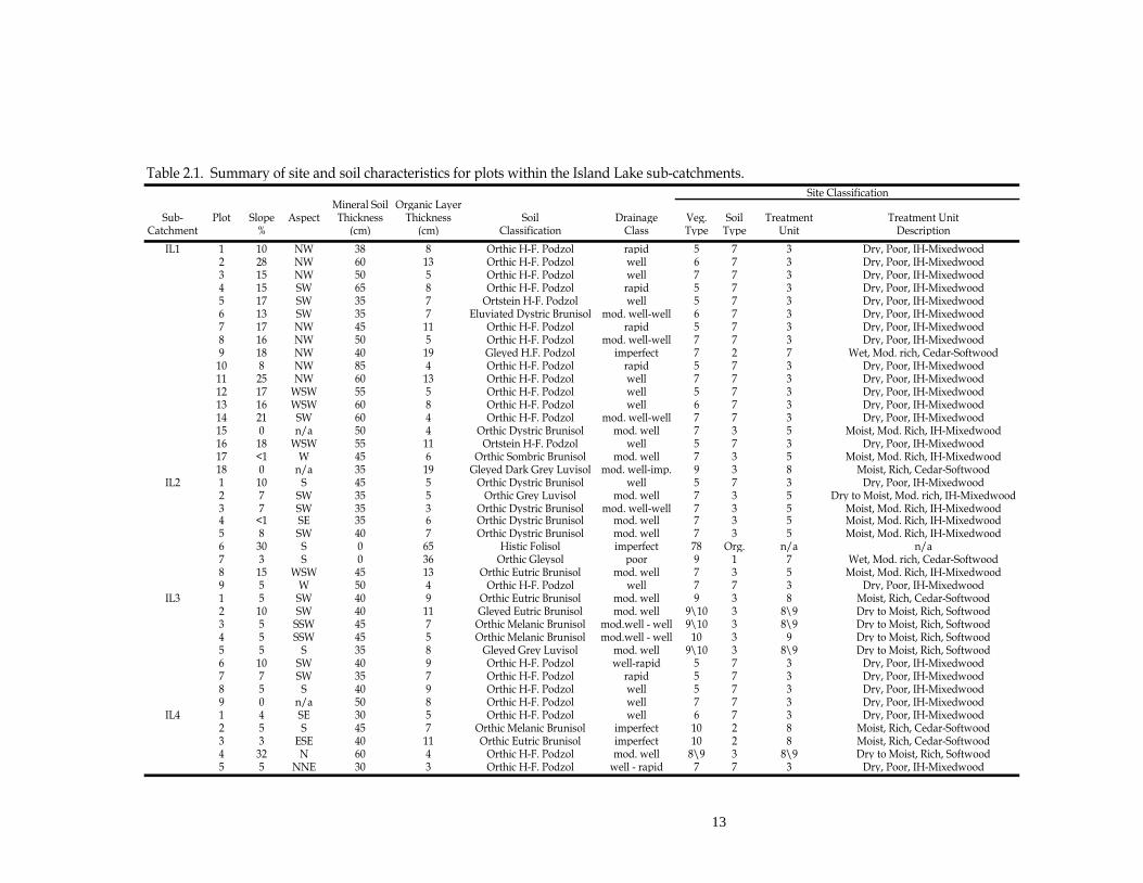
Plots at this site (Table 2.1) show a large range of variation in terms of
topography (slope, aspect), soil classification, drainage, and site classification. This
variation is characteristic of the area and can be attributed to differences in meso
and micro-scale topography and the depth and compactness of the soil and the
overall influence of these factors on lateral and vertical water flow and
accumulation conditions. The 41 plots established at this site cover a range of
aspects clockwise from east-southeast to north-northeast and slopes from 0 – 32 %.
Well to rapidly-drained ridge, upper slope, and mid-slope plots, especially those
>10 % slope or in upland positions in the drainage area, were generally humo-ferric
podzols with occasional partially cemented or ortstein subsurface layers. Lower
slope and gently sloping or terraced areas tended toward a dystric
brunisolic soil type, while moderately-well to imperfectly-drained plots in
convergent areas were generally melanic /eutric brunisols, gray luvisols or gleyed
humo-ferric podzols, indicating richer, less acidic soils. At zones of confluence of
intermittent stream channels lower in the watersheds, gleysolic and
13
Table 2.1. Summary of site and soil characteristics for plots within the Island Lake sub-catchments.
Site ClassificationMineral Soil Organic Layer
Sub- Plot Slope Aspect Thickness Thickness Soil Drainage Veg. Soil Treatment Treatment UnitCatchment % (cm) (cm) Classification Class Type Type Unit Description
IL1 1 10 NW 38 8 Orthic H-F. Podzol rapid 5 7 3 Dry, Poor, IH-Mixedwood2 28 NW 60 13 Orthic H-F. Podzol well 6 7 3 Dry, Poor, IH-Mixedwood3 15 NW 50 5 Orthic H-F. Podzol well 7 7 3 Dry, Poor, IH-Mixedwood4 15 SW 65 8 Orthic H-F. Podzol rapid 5 7 3 Dry, Poor, IH-Mixedwood5 17 SW 35 7 Ortstein H-F. Podzol well 5 7 3 Dry, Poor, IH-Mixedwood6 13 SW 35 7 Eluviated Dystric Brunisol mod. well-well 6 7 3 Dry, Poor, IH-Mixedwood7 17 NW 45 11 Orthic H-F. Podzol rapid 5 7 3 Dry, Poor, IH-Mixedwood8 16 NW 50 5 Orthic H-F. Podzol mod. well-well 7 7 3 Dry, Poor, IH-Mixedwood9 18 NW 40 19 Gleyed H.F. Podzol imperfect 7 2 7 Wet, Mod. rich, Cedar-Softwood
10 8 NW 85 4 Orthic H-F. Podzol rapid 5 7 3 Dry, Poor, IH-Mixedwood11 25 NW 60 13 Orthic H-F. Podzol well 7 7 3 Dry, Poor, IH-Mixedwood12 17 WSW 55 5 Orthic H-F. Podzol well 5 7 3 Dry, Poor, IH-Mixedwood13 16 WSW 60 8 Orthic H-F. Podzol well 6 7 3 Dry, Poor, IH-Mixedwood14 21 SW 60 4 Orthic H-F. Podzol mod. well-well 7 7 3 Dry, Poor, IH-Mixedwood15 0 n/a 50 4 Orthic Dystric Brunisol mod. well 7 3 5 Moist, Mod. Rich, IH-Mixedwood16 18 WSW 55 11 Ortstein H-F. Podzol well 5 7 3 Dry, Poor, IH-Mixedwood17 <1 W 45 6 Orthic Sombric Brunisol mod. well 7 3 5 Moist, Mod. Rich, IH-Mixedwood18 0 n/a 35 19 Gleyed Dark Grey Luvisol mod. well-imp. 9 3 8 Moist, Rich, Cedar-Softwood
IL2 1 10 S 45 5 Orthic Dystric Brunisol well 5 7 3 Dry, Poor, IH-Mixedwood2 7 SW 35 5 Orthic Grey Luvisol mod. well 7 3 5 Dry to Moist, Mod. rich, IH-Mixedwood3 7 SW 35 3 Orthic Dystric Brunisol mod. well-well 7 3 5 Moist, Mod. Rich, IH-Mixedwood4 <1 SE 35 6 Orthic Dystric Brunisol mod. well 7 3 5 Moist, Mod. Rich, IH-Mixedwood5 8 SW 40 7 Orthic Dystric Brunisol mod. well 7 3 5 Moist, Mod. Rich, IH-Mixedwood6 30 S 0 65 Histic Folisol imperfect 78 Org. n/a n/a7 3 S 0 36 Orthic Gleysol poor 9 1 7 Wet, Mod. rich, Cedar-Softwood8 15 WSW 45 13 Orthic Eutric Brunisol mod. well 7 3 5 Moist, Mod. Rich, IH-Mixedwood9 5 W 50 4 Orthic H-F. Podzol well 7 7 3 Dry, Poor, IH-Mixedwood
IL3 1 5 SW 40 9 Orthic Eutric Brunisol mod. well 9 3 8 Moist, Rich, Cedar-Softwood2 10 SW 40 11 Gleyed Eutric Brunisol mod. well 9\10 3 8\9 Dry to Moist, Rich, Softwood3 5 SSW 45 7 Orthic Melanic Brunisol mod.well - well 9\10 3 8\9 Dry to Moist, Rich, Softwood4 5 SSW 45 5 Orthic Melanic Brunisol mod.well - well 10 3 9 Dry to Moist, Rich, Softwood5 5 S 35 8 Gleyed Grey Luvisol mod. well 9\10 3 8\9 Dry to Moist, Rich, Softwood6 10 SW 40 9 Orthic H-F. Podzol well-rapid 5 7 3 Dry, Poor, IH-Mixedwood7 7 SW 35 7 Orthic H-F. Podzol rapid 5 7 3 Dry, Poor, IH-Mixedwood8 5 S 40 9 Orthic H-F. Podzol well 5 7 3 Dry, Poor, IH-Mixedwood9 0 n/a 50 8 Orthic H-F. Podzol well 7 7 3 Dry, Poor, IH-Mixedwood
IL4 1 4 SE 30 5 Orthic H-F. Podzol well 6 7 3 Dry, Poor, IH-Mixedwood2 5 S 45 7 Orthic Melanic Brunisol imperfect 10 2 8 Moist, Rich, Cedar-Softwood3 3 ESE 40 11 Orthic Eutric Brunisol imperfect 10 2 8 Moist, Rich, Cedar-Softwood4 32 N 60 4 Orthic H-F. Podzol mod. well 8\9 3 8\9 Dry to Moist, Rich, Softwood5 5 NNE 30 3 Orthic H-F. Podzol well - rapid 7 7 3 Dry, Poor, IH-Mixedwood

14
organic soils were present, typical of areas of high flow accumulation in this
landscape. The effective rooting depth ranged from 30 to 50 cm with deeper soils
occurring on steeper side and foot-slopes and more shallow soils on ridges and
gentle-sloping areas. Overall, site classifications carried out at the sample plots
agreed closely with the drainage and soil types found, as well as with the
dominant tree species.
Gounamitz Lake Site
In contrast to the Island Lake project site, plots at the Gounamitz Lake
site are more homogeneous in soil, drainage and vegetation characteristics (Table
2.2). Of 36 plots sampled across this site, 19 were described as orthic humo-ferric
podzols, 12 as orthic ferro-humic podzols, and the remaining 5 were orthic
dystric brunisols. In general, the podzolic soils were rapidly- to well-drained
and were characterised by a strong eluvial A layer while the brunisols were
moderately well to well-drained. Site classification results showed a similar
degree of homogeneity; sites were classified as dry, rich, hardwood with little
variation in dominant tree species, shrub species or soil type. Slope values
ranged from 0 % to 15 % in the steepest areas and aspects were mainly north
facing with values ranging between west and east. The most deeply rooted
plots, as at Island Lake, occurred on the steeper side slopes while shallow-rooted
plots occurred mainly on flat hilltops, where the bedrock was close to the surface.

15
Table 2.2. Summary of site and soil characteristics for plots within the Gounamitz Lake sub-catchments.
Site ClassificationMineral Soil Organic Layer
Sub- Plot Slope Aspect Thickness Thickness Soil Drainage Veg. Soil Treatment Treatment Unit
Catchment % (cm) (cm) Classification Class Type Type Unit Description
GL1 1 7 NNE 46 4 Orthic H.-F. Podzol Well 11 6 11 Dry-Moist, rich, hardwood
2 3 NNW 51 6 Orthic H.-F. Podzol Well 11 6 11 Dry-Moist, rich, hardwood
3 3 NNE 70 5 Orthic Dystric Brunisol Well 12 6 12 Very dry, mod. rich, hardwood
4 5 N 54 4 Orthic H.-F. Podzol Well 11 7 12 Very dry, mod. rich, hardwood
5 8 NE 63 1 Orthic H.-F. Podzol Well-Mod.Well 11 6 11 Dry-Moist, rich, hardwood
6 4 NNE 43 6 Orthic Dystric Brunisol Mod. Well 12 2 11 Dry-Moist, rich, hardwood
7 4 N 54 4 Orthic H.-F. Podzol Rapid 11 7 12 Very dry, mod. rich, hardwood
8 10 NNE 55 5 Orthic H.-F. Podzol Well 11 6 11 Dry-Moist, rich, hardwood
9 4 NNE 57 6 Orthic H.-F. Podzol Well 11 6 11 Dry-Moist, rich, hardwood
10 10 NNE 58 3 Orthic Dystric Brunisol Mod. Well 12 2 11 Dry-Moist, rich, hardwood
GL2 1 3 NNW 45 4 Orthic H.-F. Podzol Rapid 11 7 12 Very dry, mod. rich, hardwood
2 3 NNW 42 2 Orthic F.-H. Podzol Rapid 11 7 12 Very dry, mod. rich, hardwood
3 8 N 54 3 Orthic F.-H. Podzol Well-Rapid 11 7 12 Very dry, mod. rich, hardwood
4 6 N 54 4 Orthic F.-H. Podzol Well 11 6 11 Dry-Moist, rich, hardwood
5 1 NE 54 4 Orthic F.-H. Podzol Well 11 6 11 Dry-Moist, rich, hardwood
6 1 NE 59 4 Orthic F.-H. Podzol Rapid 11 7 12 Very dry, mod. rich, hardwood
7 5 N 43 3 Orthic H.-F. Podzol Rapid 11 7 12 Very dry, mod. rich, hardwood
8 8 NE 53 3 Orthic H.-F. Podzol Well 11 6 11 Dry-Moist, rich, hardwood
9 10 NE 65 5 Orthic H.-F. Podzol Well 11 6 11 Dry-Moist, rich, hardwood
10 7 NNE 50 5 Orthic H.-F. Podzol Well 12 6 12 Very dry, mod. rich, hardwood
GL3 1 6 E 52 2 Orthic H.-F. Podzol Well-Rapid 11 6 11 Dry-Moist, rich, hardwood
2 2 NE 44 4 Orthic H.-F. Podzol Well 11 6 11 Dry-Moist, rich, hardwood
3 10 ENE 48 3 Orthic F.-H. Podzol Well-Rapid 11 7 12 Very dry, mod. rich, hardwood4 15 ENE 78 3 Orthic F.-H. Podzol Rapid 11 7 12 Very dry, mod. rich, hardwood
5 5 NE 58 3 Orthic F.-H. Podzol Well 11 6 11 Dry-Moist, rich, hardwood
6 1 N 58 3 Orthic F.-H. Podzol Well-Rapid 11 6 11 Dry-Moist, rich, hardwood
7 8 NW 48 3 Orthic F.-H. Podzol Well 11 6 11 Dry-Moist, rich, hardwood
8 3 NE 55 5 Orthic F.-H. Podzol Well 11 6 11 Dry-Moist, rich, hardwood
9 13 W 64 4 Orthic F.-H. Podzol Well 11 6 11 Dry-Moist, rich, hardwood
GL4 1 0 n/a 46 4 Orthic H.-F. Podzol Well 11 6 11 Dry-Moist, rich, hardwood
2 2 ENE 50 5 Orthic H.-F. Podzol Well 11 6 11 Dry-Moist, rich, hardwood
3 3 ENE 43 3 Orthic H.-F. Podzol Well 11 6 11 Dry-Moist, rich, hardwood
4 8 NE 45 5 Orthic Dystric Brunisol Well 12 6 12 Very dry, mod. rich, hardwood
5 4 NE 44 4 Orthic Dystric Brunisol Well 12 6 12 Very dry, mod. rich, hardwood
6 13 NE 46 6 Orthic H.-F. Podzol Well 12 6 12 Very dry, mod. rich, hardwood
7 5 NNE 42 2 Orthic H.-F. Podzol Well 11 6 11 Dry-Moist, rich, hardwood

16 16
CHAPTER 3
DERIVING WATER FLOW AND ACCUMULATION ATTRIBUTES:
A CONSIDERATION OF SCALE AND TOPOGRAPHIC COMPLEXITY
INTRODUCTION
Topographic attributes such as slope, flow accumulation, and slope
curvature are indices used to characterise morphologically or hydrologically
significant landscape features influencing soil and biological processes while
maintaining adequate realism. This abstraction is especially useful in a spatial
context where complexity can be overwhelming. Digital Elevation Models
(DEM’s) have made possible the automatic derivation of these quantitative
topographic indices; both Speight (1974) and Moore et al. (1991) provide excellent
overviews of the derivation, calculation and importance of a range of topographic
attributes. However, both the quality and the resolution of the elevation data
used to create DEM’s can have many implications for topographic attributes
derived from them, and are often not addressed.
As such, the objective of this chapter is to provide a rationale for the
choice and derivation of the topographic indices to be used with respect to the
scale and accuracy of available New Brunswick provincial elevation data.
Specifically, this chapter examines: (1) the assignment of topographic attributes
using a) New Brunswick elevation data and b) a set of “best estimate” criteria
17 17
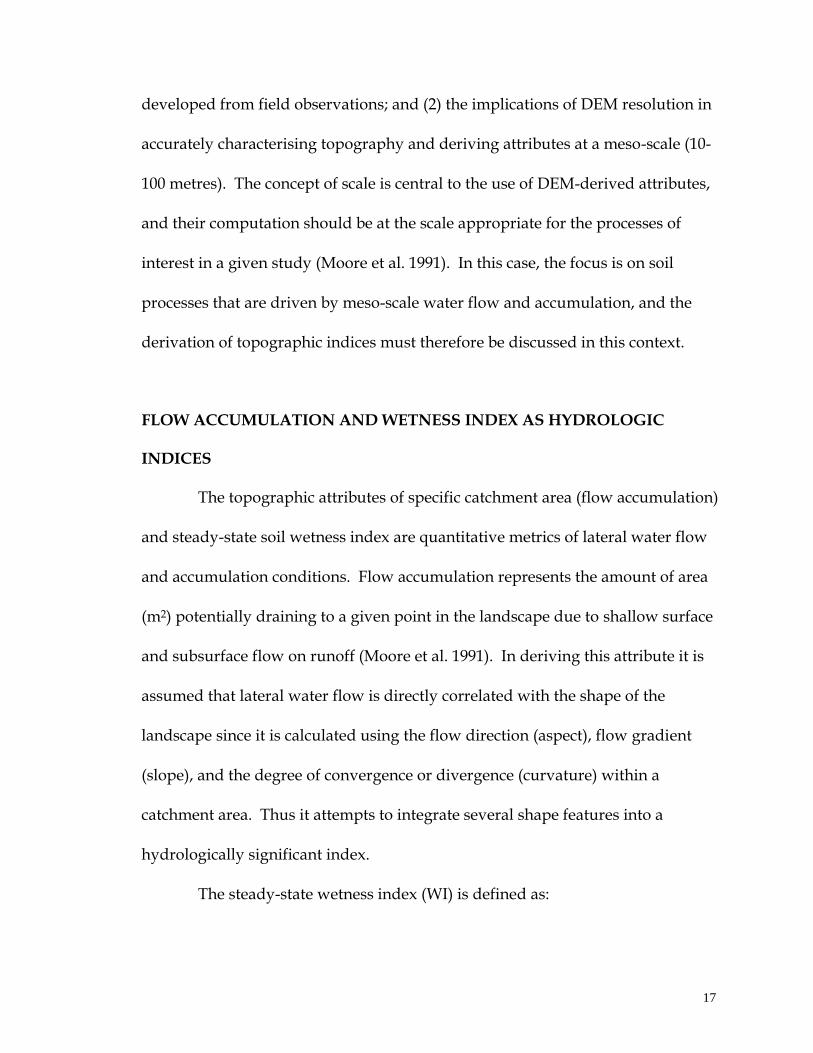
developed from field observations; and (2) the implications of DEM resolution in
accurately characterising topography and deriving attributes at a meso-scale (10-
100 metres). The concept of scale is central to the use of DEM-derived attributes,
and their computation should be at the scale appropriate for the processes of
interest in a given study (Moore et al. 1991). In this case, the focus is on soil
processes that are driven by meso-scale water flow and accumulation, and the
derivation of topographic indices must therefore be discussed in this context.
FLOW ACCUMULATION AND WETNESS INDEX AS HYDROLOGIC
INDICES
The topographic attributes of specific catchment area (flow accumulation)
and steady-state soil wetness index are quantitative metrics of lateral water flow
and accumulation conditions. Flow accumulation represents the amount of area
(m2) potentially draining to a given point in the landscape due to shallow surface
and subsurface flow on runoff (Moore et al. 1991). In deriving this attribute it is
assumed that lateral water flow is directly correlated with the shape of the
landscape since it is calculated using the flow direction (aspect), flow gradient
(slope), and the degree of convergence or divergence (curvature) within a
catchment area. Thus it attempts to integrate several shape features into a
hydrologically significant index.
The steady-state wetness index (WI) is defined as:
18 18
where a is the flow accumulation for a given cell and tan ß is the local slope
gradient (Moore et al. 1991). This attribute is a spatial index of potential zones of
saturation and integrates the effect of slope gradient and flow accumulation such
that areas of low slope gradient (i.e. ridge tops and flat areas) and high flow
situations (i.e. convergent zones or confluence points) would produce higher WI
values since these areas potentially receive and hold more water.
Like flow accumulation, WI assumes that piezometric gradients are
reflected by topography, which parallels subsurface geometry, and that
transmissivity is uniform across an area (O’Loughlin 1986; Moore 1996).
Admittedly, spatial differences in porosity and transmissivity can occur due to
variable soil textures, coarse fragment content, soil depths, and bulk densities.
These differences, however, are hard to characterise accurately and in areas
where annual precipitation outweighs evapotranspiration, as is the case here,
topography is assumed to be the driving influence on water flow characteristics.
The calculation of flow accumulation is derived through the modelling of
ephemeral flow networks and has been the focus of numerous studies (e.g.
O’Callahan and Mark 1984; Mark 1988; Tarboton et al. 1991; Quinn et al. 1991;
Jenson 1991; Costa-Cabral and Burges 1994). Wetness index has been used in
hydrological research studies investigating controls of soil moisture (Burt and
WIa
ln
tan
19 19
Butcher 1985,1986; Moore et al. 1988) and is a key component of Beven and
Kirkby’s (1979) flood forecasting model, TOPMODEL. Despite the demonstrated
utility of flow accumulation and wetness index in hydrological research and the
knowledge that water flow greatly influences soil properties, these indices have
rarely been applied in soil investigations.
METHODS
Deriving Topographic Attribute Values From Available DEM Data
Irregularly-spaced elevation measurements with an average spacing of
approximately 70m were obtained from the province of New Brunswick for the
Island Lake and Gounamitz Lake areas. From these irregular grids, regular grid
DEM’s were interpolated to a resolution of 15 m with the creation of Delaunay
Triangles and subsequent fitting of smooth surfaces using a bivariate fifth order
polynomial expression (Vertical Mapper v.2 1998). Costa-Cabral and Burges’
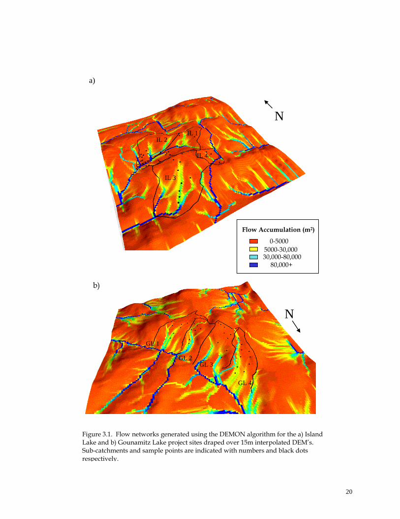
(1994) DEMON (digital elevation model network extraction) algorithm is used
here to derive flow networks (Figure 3.1) and to calculate flow accumulation
values. With this algorithm, flow is weighted and dispersed among grid cells
instead of flowing into only one grid cell, as with algorithms such as the D8 and
Rho8 methods. Moore (1996), in comparing flow routing algorithms through
sensitivity analyses, concluded that the computation of flow accumulation is
highly dependent on the algorithm used and that distributed flow models such as
DEMON are more realistic and preferable to the simple nearest-neighbour
20 20
Figure 3.1. Flow networks generated using the DEMON algorithm for the a) Island Lake and b) Gounamitz Lake project sites draped over 15m interpolated DEM’s. Sub-catchments and sample points are indicated with numbers and black dots respectively.
a)
b)
N
N
0-5000 5000-30,000 30,000-80,000
80,000+
Flow Accumulation (m2)
IL 1
IL 4
IL 3
IL 2
GL 3
GL 4
GL 2
GL 1

21 21
algorithms (i.e. D8 and Rho8). The steady-state wetness index (WI) was derived
as a combination of cell-specific flow accumulation and slope, calculated directly
from the DEM for each cell using a 3X3 submatrix of elevation points (e.g.
Zevenbergen and Thorne 1987). Values for these topographic attributes were
derived for each plot by overlaying cell-specific values and plot locations.
Deriving Expected Values as a Best Estimate
Upon exploratory 3-D rendering of the provincial DEM data, it was clear
that certain field-observed terrain features could not be resolved with this
elevation data set. Consequently, known flow paths, and plots established in
these paths, did not coincide properly with modelled flow networks, resulting in
errors in calculated flow accumulation values. As such, I developed a set of
criteria, a priori, for deriving plot-specific “expected values” for flow
accumulation to be used as a best-estimate comparison.
Expected flow accumulation assignments were primarily based on
observations of plot specific topographic conditions. I used observed terrain
convergence/divergence and the overall location of each plot along a given flow
channel or slope (i.e. landscape position) as field-level indicators of the potential
flow accumulation at a point. Subsequently, I assigned a specific flow
accumulation value (m2) at each point by referencing the flow accumulation value of
the nearest comparable cell along the modelled flow path. This approach effectively
aimed to correct the bias introduced by the coarseness of the DEM. In using this

22 22
approach, I assumed that water flowing along a given modelled flow path was
not redirected or obstructed in any way.
It could be argued that expected values were assigned somewhat
arbitrarily. However, in lieu of accurate topographic data, I contend that these
corrections provide valid flow accumulation comparisons based on field
observation and best-available DEM data.
Three flow accumulation situations appeared to exist, defined as:
1. Low Potential Flow Accumulation (500 – 2000 m2 drainage):
These plots were located on divergent ridge positions or along shorter, even
slopes and obviously accumulating little up-slope water.
Assigned flow accumulation values reflected the estimated direct up-slope
area draining to that point along the local slope gradient.
2. High Potential Flow Accumulation (15000 – 80000 m2 drainage):
These plots were indicative of wet conditions in the field (seepage zones,
depressions, toe-slopes, confluence points of ephemeral flow channels) or
were lower in the watershed and appeared to be situated along major field-
observed flow channels.
Values were estimated using the most representative, nearest flow line
convergence point portrayed by the DEMON flow algorithm. In most cases,
the locations of modelled flow lines were displaced from their actual location
in the field but were generally representative.

23 23
3. Moderate Potential Flow Accumulation (2000 – 15000 m2 drainage):
These plots, not falling into either above category, were usually found along
mild but even slope gradients, at the toe of shorter side-slopes or at mid-
watershed positions and were most difficult to estimate.
Overall, values were assigned to reflect the degree of convergence or
divergence, the effective moisture condition and its overall macro-scale
position in the watershed and were calculated based on the modelled flow
area draining to that locale.
At the Gounamitz site, topographic convergence and divergence was subtle, and
assignments of expected values relied more heavily on modelled flow networks.
Consequently, each successive plot situated down a given flow line was assigned
a progressively higher expected value for flow accumulation; these values
essentially reflected the overall landscape position of each plot in the catchment.
Expected wetness index values were calculated as a combination of
expected flow accumulation and field-measured percent slope gradient at each
plot. DEM-derived and expected values were compared and assessed in the
context of data quality and scale.

24 24
RESULTS AND DISCUSSION
Evaluation of DEM-derived Attributes and the Influence of DEM Scale
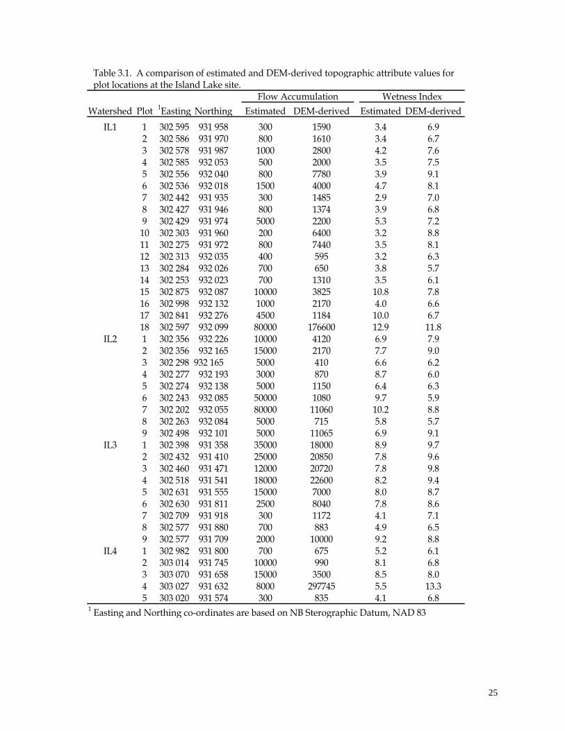
There is a clear disparity between DEM-derived topographic attribute
values and estimated values assigned to each plot using proposed criteria at both
the Island Lake (Table 3.1) and Gounamitz Lake (Table 3.2) sites. I speculate that
these differences are largely due to the inability to resolve finer-scale landforms
with readily available elevation data.
At Island Lake the topography is undulating and distance between
pronounced hummocks and depressions are, at times, much less than the 70 m
resolution of the NB elevation data. Consequently, any major landform occurring
at finer intervals were likely misrepresented resulting in substantial differences
between DEM-derived and expected values for topographic attributes. For
example (Figure 3.1a), the lower sections of watershed IL1 and IL 2 were not
properly resolved although clear flow channels defined these sub-catchments and
guided the placement of plots in the field. In addition, catchment IL4 shows the
modelled flow network exiting the watershed south through a ridge area, instead
of flowing south-east towards the nearest stream; there is also a small perched
pond in this catchment that could not be delineated using the DEM. Only plots in
IL3 and in the upper sections of IL 1 appeared to have any correspondence
between DEM-derived and expected values.
25 25
Table 3.1. A comparison of estimated and DEM-derived topographic attribute values for plot locations at the Island Lake site.
Flow Accumulation Wetness Index
Watershed Plot 1Easting Northing Estimated DEM-derived Estimated DEM-derived
IL1 1 302 595 931 958 300 1590 3.4 6.92 302 586 931 970 800 1610 3.4 6.73 302 578 931 987 1000 2800 4.2 7.64 302 585 932 053 500 2000 3.5 7.55 302 556 932 040 800 7780 3.9 9.16 302 536 932 018 1500 4000 4.7 8.17 302 442 931 935 300 1485 2.9 7.08 302 427 931 946 800 1374 3.9 6.89 302 429 931 974 5000 2200 5.3 7.210 302 303 931 960 200 6400 3.2 8.811 302 275 931 972 800 7440 3.5 8.112 302 313 932 035 400 595 3.2 6.313 302 284 932 026 700 650 3.8 5.714 302 253 932 023 700 1310 3.5 6.115 302 875 932 087 10000 3825 10.8 7.816 302 998 932 132 1000 2170 4.0 6.617 302 841 932 276 4500 1184 10.0 6.718 302 597 932 099 80000 176600 12.9 11.8
IL2 1 302 356 932 226 10000 4120 6.9 7.92 302 356 932 165 15000 2170 7.7 9.03 302 298 932 165 5000 410 6.6 6.24 302 277 932 193 3000 870 8.7 6.05 302 274 932 138 5000 1150 6.4 6.36 302 243 932 085 50000 1080 9.7 5.97 302 202 932 055 80000 11060 10.2 8.88 302 263 932 084 5000 715 5.8 5.79 302 498 932 101 5000 11065 6.9 9.1
IL3 1 302 398 931 358 35000 18000 8.9 9.72 302 432 931 410 25000 20850 7.8 9.63 302 460 931 471 12000 20720 7.8 9.84 302 518 931 541 18000 22600 8.2 9.45 302 631 931 555 15000 7000 8.0 8.76 302 630 931 811 2500 8040 7.8 8.67 302 709 931 918 300 1172 4.1 7.18 302 577 931 880 700 883 4.9 6.59 302 577 931 709 2000 10000 9.2 8.8
IL4 1 302 982 931 800 700 675 5.2 6.12 303 014 931 745 10000 990 8.1 6.83 303 070 931 658 15000 3500 8.5 8.04 303 027 931 632 8000 297745 5.5 13.35 303 020 931 574 300 835 4.1 6.8
1 Easting and Northing co-ordinates are based on NB Sterographic Datum, NAD 83
26 26
Table 3.2. A comparison of estimated and DEM-derived topographic attribute values for plot locations at the Gounamitz Lake site.
Flow Accumulation Wetness Index
Watershed Plot1Easting Northing Estimated DEM-derived Estimated DEM-derived
GL1 1 213 721 919 429 10000 10400 7.3 9.72 213 724 919 533 20000 1735 8.8 7.53 213 751 919 603 30000 2260 9.2 7.34 213 790 919 676 45000 5700 9.1 8.15 213 859 919 777 60000 16950 8.9 9.76 213 905 919 835 80000 10000 9.9 8.97 213 686 919 648 2000 775 6.2 6.38 213 698 919 713 5000 3150 6.2 7.39 213 736 919 781 10000 2355 7.8 7.110 213 815 919 848 20000 9170 7.6 9.2
GL2 1 213 880 919 144 500 270 5.1 6.32 213 859 919 177 500 950 5.1 6.83 213 829 919 228 500 1520 4.1 7.24 213 859 919 316 3000 1745 6.2 7.75 213 962 919 420 7500 4700 6.6 7.66 213 729 919 305 1000 3600 4.6 8.97 213 793 919 360 500 2655 4.6 8.28 213 844 919 404 2000 2125 5.5 7.69 213 903 919 552 20000 4500 7.6 7.510 213 975 919 602 35000 5500 8.5 8.1
GL3 1 214 034 919 053 1000 615 5.1 6.92 214 082 919 040 3000 2000 7.3 7.43 214 131 919 087 5000 1170 6.2 6.74 214 104 919 155 500 1700 3.5 7.15 214 170 919 150 8000 3545 7.4 7.56 214 157 919 033 2000 2170 5.3 7.67 214 209 919 119 5000 15500 10.1 9.58 214 261 919 258 45000 3730 9.6 7.99 214 277 919 305 1000 25325 4.3 9.5
GL4 1 214 059 918 935 500 262 7.8 6.42 214 131 918 935 1000 855 6.9 6.83 214 237 918 995 5000 3055 7.4 8.34 214 329 919 043 20000 5400 7.8 8.45 214 426 919 099 30000 16000 8.9 9.26 214 471 919 159 45000 21870 8.1 9.87 214 308 918 993 1000 5490 5.3 8.8
1 Easting and Northing co-ordinates are based on NB Sterographic Datum, NAD 83
27 27
At the Gounamitz Lake site, the topography was more subdued and
elevation differences between areas were subtle; DEM resolution and accuracy
would therefore be crucial in accurately depicting modelled flow channels and
deriving water flow attributes. Many of the plots at this site were successively
placed along perceived flow lines which, upon examination of Figure 3.1b,
appeared to be fairly representatively modelled. However, it was obvious that
there was some displacement between actual channel/plot locations and
modelled flow networks due to the interpolation to a 15 m grid resolution, and
ultimately resulted in incorrect calculation of plot-specific flow accumulation.
Primary attributes such as slope and flow accumulation are very sensitive
to grid resolution (Moore 1996) since their calculation requires the shape of a
given point in space be depicted accurately as a grid-cell or a combination of
adjacent cells within the DEM. Wilson et al. (1998), for example, demonstrated
that variations of only 0.05 % in mean elevations between two DEM grids
resulted in substantial differences in calculated terrain attributes for a 20 ha farm
field.
Further, the “mismatching” of study scale and data structure and resolution,
though rarely considered in studies applying digitally-derived data, can be a
significant problem (Zhang and Montgomery 1994). In a study of a spatial scale
similar to this one, Zhu et al. (1997) found that a 7.5 minute quadrangle USGS
DEM (25 m north-south grid spacings with 150 m between transects) was not
sufficient to characterise local landforms and soil transmissivity in a 173 ha
28 28
watershed of relatively subtle topography. Dietrich et al. (1993), using data of a
similar resolution, were unable to delineate accurate channel networks in a study
of erosion thresholds for a 120 ha watershed. In a study of geomorphological
landform analysis, Dikau (1989) stated that DEM grids finer than 40 or 50 m were
necessary to produce accurate geomorphological maps of micro and meso-relief.
Similar to the above studies, the interpolation of elevation data in this
investigation to a scale four times smaller than the original data greatly
influenced the depiction of topography and the calculation of attribute values and
was generally inadequate.
Estimated Values
Verifying the accuracy of attributes assigned using either the provincial
DEM or the presented criteria would be a difficult task since it would require
direct quantitative measurement of surface and subsurface water flow and
distribution. However, studies that have correlated DEM-derived topographic
attribute values to site-specific soil water properties (e.g. Burt and Butcher
1985,1986; O’Loughlin 1986; Moore et al. 1988) have provided some measure of
validation of their practical application; this justification is important although
most studies have used derived topographic attributes with little consideration of
their accuracy in a given landscape.
A range of drainage classes from rapid to poor, indicating the average
wetness at each plot, correlated strongly and positively with estimated values for
29 29
both flow accumulation and wetness index at Island Lake (Figure 3.2). Plots that
were well to moderately-well drained displayed the most variability; this is not
surprising since these areas were situated at both dry divergent positions and
convergent positions with varying amounts of estimated up-slope drainage.
At the Gounamitz site, plots were all rapidly to well-drained, indicating
relatively fast vertical drainage relative to lateral water flow. Topographic
attributes, however, showed three distinct groups based on soil class. Mean
topographic attribute values were clearly different among Orthic Ferro-Humic
Podzol, Orthic Humo-Ferric Podzol, and Orthic Dystric Brunisol (Figure 3.3)
groups. Although plot-specific water flow was not expressed in drainage
conditions, results indicated that obvious spatial differences existed, and that
these differences were correlated with expected flow accumulation conditions.
Soil development is widely known to be strongly influenced by both
lateral and vertical water flow. At this site, the influence of vertical water flow
was clearly expressed in the contrasting soil profiles found; I propose that the
spatial arrangement of these soil types, as indicated here, was most likely the
result of lateral water flow conditions from up-slope to down-slope positions at a
meso-scale. This effect is subtle, but the increase in bulk density lower in the
profile would encourage some subsurface lateral flow in addition to the overland
flow that would probably occur at peak flow periods (O’Loughlin 1986).
30 30
4
8
12
1 2 3 4 5
Wetness Index = 1.47 + 1.892 * Drainage Class
2.5
3.5
4.5
5.5
1 2 3 4 5
Drainage Class
Flow Accumulation = 1.869 + .629 * Drainage Class
r = 0.70
r = 0.82
Drainage Class
1 - Rapid 2 - Well 3 - Moderately Well 4 - Imperfect 5 - Poor
Figure 3.2. Correlation between expected values for topographic attributes and drainage class at Island Lake. Best-fit regression equations have been included.
Lo
g F
low
Ac
cu
mu
lati
on
(m
2)
We
tne
ss I
nd
ex
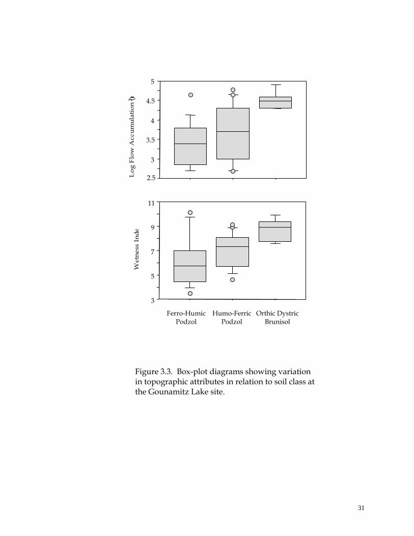
31 31
2.5
3
3.5
4
4.5
5
3
5
7
9
11
Ferro-Humic Podzol
Humo-Ferric Podzol
Orthic Dystric Brunisol
Figure 3.3. Box-plot diagrams showing variation in topographic attributes in relation to soil class at the Gounamitz Lake site.
We
tne
ss I
nd
ex
Lo
g F
low
Ac
cu
mu
lati
on
(m
2)

32 32
SUMMARY
Results presented here illustrate the need for caution in using DEM-
derived data in ecological studies where either the accuracy of the DEM is in
question or when the study scale is finer than that of the DEM (Quinn et al. 1991;
Moore 1996; Zhang and Montgomery 1994; Iverson et al. 1997; Brasington and
Richards 1998). Results suggested that readily available New Brunswick
Provincial elevation data were inadequate for characterising topography and
deriving topographic attributes at a local, plot-specific scale.
Estimated topographic attribute values, however, appeared valid to the
extent that they reflected the relative drainage conditions and soil development
conditions at the Island Lake and Gounamitz Lake sites respectively; both
characteristics are widely known to be strongly influenced by water flow and
accumulation. In contrast, DEM-derived attributes showed no apparent
relationship to drainage class or soil development at either site.
33 33
CHAPTER 4
THE INFLUENCE OF TOPOGRAPHY ON SOIL PHYSICAL
PROPERTY DISTRIBUTION
INTRODUCTION
Texture, coarse fragment content and depth are a few of the intermediary
soil physical properties that ultimately determine spatial differences in soil
fertility. There is little question that the relatively steady-state-quality of soil
physical parameters make them useful as indicators of complex soil processes
that are difficult to measure spatially and are highly variable temporally.
Consequently, measures of soil physical properties have been used extensively to
model general aeration, moisture and nutrient regimes and forest productivity
(Kimmins 1987). Soil-landscape investigations that lead to increased
understanding of the possible mechanisms of physical property distributions
across different landscapes are therefore extremely valuable.
Physical soil characteristics are the result of a host of influences that have
acted on local surficial geology over long periods of time and may be largely
attributed to: (1) the composition and mode of deposition of the soil parent
material and (2) local topographic influences on surface and subsurface water
flow and resultant spatial differences in weathering, erosional and horizonation
processes (Gerrard 1981). As a result of the complexity of these combined
influences, soil textures and depths are difficult to characterise; averaged soil map

34 34
unit descriptions often do not provide an accurate depiction of meso-scale
distributions of soil physical properties, particularly in terrain where lateral
surface and subsurface water flow causes differential weathering and transport of
fine particles across space.
The objective of this chapter is to investigate potential predictive
relationships between several metrics of later water flow and soil physical
characteristics at the Island Lake and Gounamitz Lake sites; relationships are
examined by way of regression analysis and comparisons made between sites.
BACKGROUND
Potential relationships between topography and distributions of soil
physical characteristics have been the focus of numerous soil science studies
aiming to understand soil formation processes or to improve local soil mapping
efforts. A summary of similar, frequently-cited investigations at a scale
comparable to this study (Table 4.1) illustrates the diversity of investigations in
terms of: (1) substrate and site characteristics; (2) the approach taken in
characterising topography and; (3) the method of analysis of soil-landscape
relationships.
Of the 14 studies summarised, the majority addressed the influence of
topography on measured soil properties by partitioning the area into topographic
classes or positions, delineated either arbitrarily or by using slope morphology
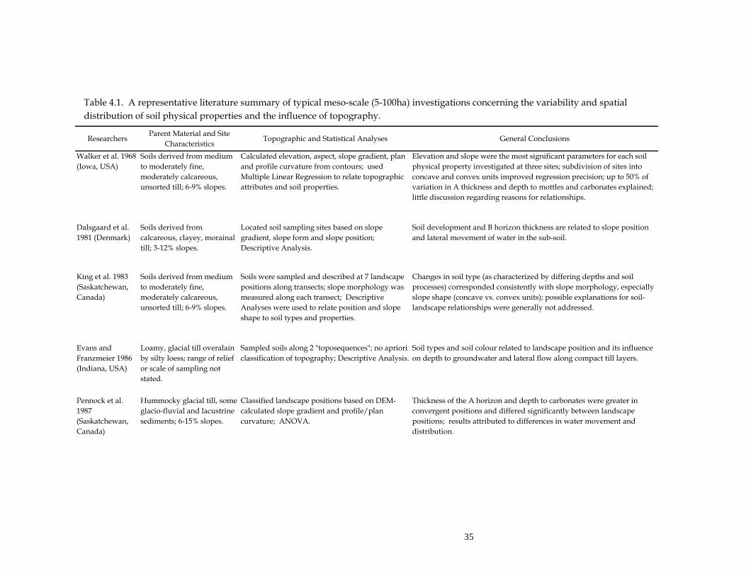
35
Table 4.1. A representative literature summary of typical meso-scale (5-100ha) investigations concerning the variability and spatial
distribution of soil physical properties and the influence of topography.
ResearchersParent Material and Site
CharacteristicsTopographic and Statistical Analyses General Conclusions
Walker et al. 1968
(Iowa, USA)
Soils derived from medium
to moderately fine,
moderately calcareous,
unsorted till; 6-9% slopes.
Calculated elevation, aspect, slope gradient, plan
and profile curvature from contours; used
Multiple Linear Regression to relate topographic
attributes and soil properties.
Elevation and slope were the most significant parameters for each soil
physical property investigated at three sites; subdivision of sites into
concave and convex units improved regression precision; up to 50% of
variation in A thickness and depth to mottles and carbonates explained;
little discussion regarding reasons for relationships.
Dalsgaard et al.
1981 (Denmark)
Soils derived from
calcareous, clayey, morainal
till; 3-12% slopes.
Located soil sampling sites based on slope
gradient, slope form and slope position;
Descriptive Analysis.
Soil development and B horizon thickness are related to slope position
and lateral movement of water in the sub-soil.
King et al. 1983
(Saskatchewan,
Canada)
Soils derived from medium
to moderately fine,
moderately calcareous,
unsorted till; 6-9% slopes.
Soils were sampled and described at 7 landscape
positions along transects; slope morphology was
measured along each transect; Descriptive
Analyses were used to relate position and slope
shape to soil types and properties.
Changes in soil type (as characterized by differing depths and soil
processes) corresponded consistently with slope morphology, especially
slope shape (concave vs. convex units); possible explanations for soil-
landscape relationships were generally not addressed.
Evans and
Franzmeier 1986
(Indiana, USA)
Loamy, glacial till overalain
by silty loess; range of relief
or scale of sampling not
stated.
Sampled soils along 2 "toposequences"; no apriori
classification of topography; Descriptive Analysis.
Soil types and soil colour related to landscape position and its influence
on depth to groundwater and lateral flow along compact till layers.
Pennock et al.
1987
(Saskatchewan,
Canada)
Hummocky glacial till, some
glacio-fluvial and lacustrine
sediments; 6-15% slopes.
Classified landscape positions based on DEM-
calculated slope gradient and profile/plan
curvature; ANOVA.
Thickness of the A horizon and depth to carbonates were greater in
convergent positions and differed significantly between landscape
positions; results attributed to differences in water movement and
distribution.
36 36
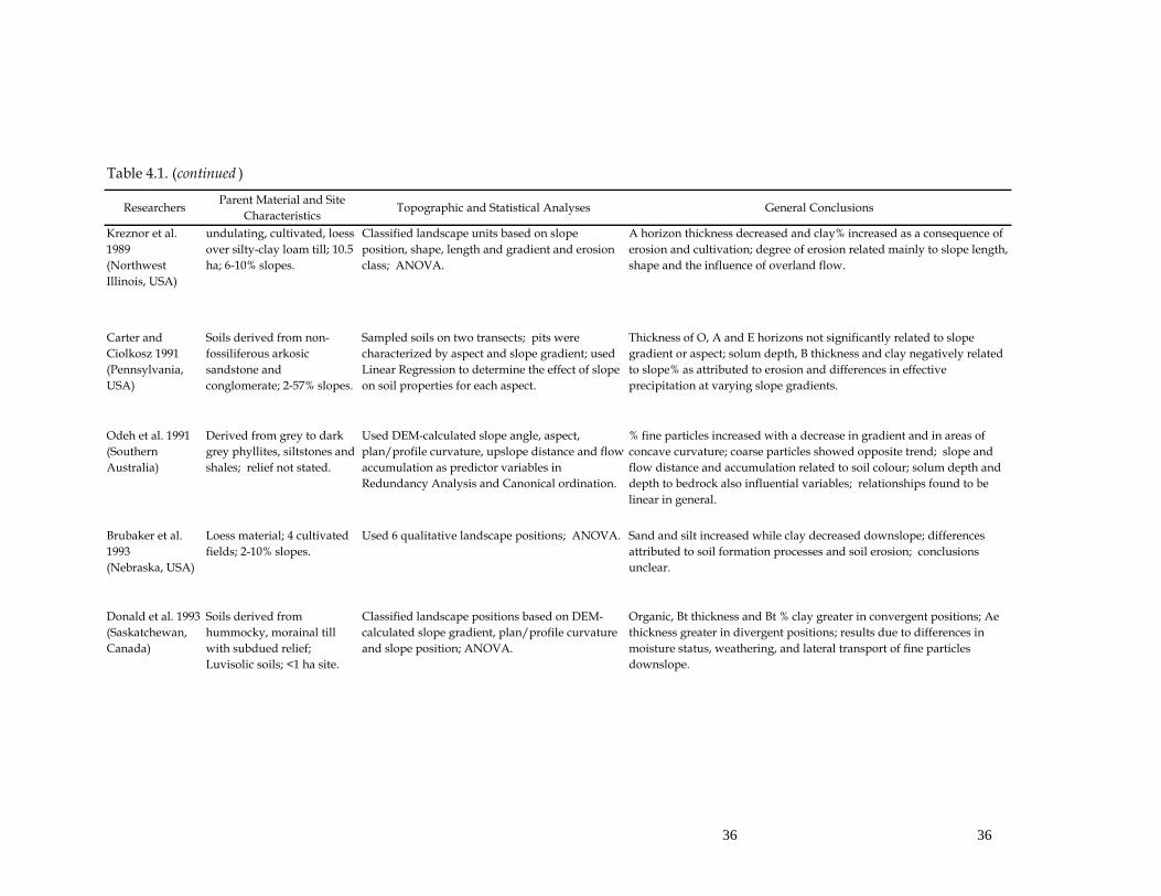
Table 4.1. (continued )
ResearchersParent Material and Site
CharacteristicsTopographic and Statistical Analyses General Conclusions
Kreznor et al.
1989
(Northwest
Illinois, USA)
undulating, cultivated, loess
over silty-clay loam till; 10.5
ha; 6-10% slopes.
Classified landscape units based on slope
position, shape, length and gradient and erosion
class; ANOVA.
A horizon thickness decreased and clay% increased as a consequence of
erosion and cultivation; degree of erosion related mainly to slope length,
shape and the influence of overland flow.
Carter and
Ciolkosz 1991
(Pennsylvania,
USA)
Soils derived from non-
fossiliferous arkosic
sandstone and
conglomerate; 2-57% slopes.
Sampled soils on two transects; pits were
characterized by aspect and slope gradient; used
Linear Regression to determine the effect of slope
on soil properties for each aspect.
Thickness of O, A and E horizons not significantly related to slope
gradient or aspect; solum depth, B thickness and clay negatively related
to slope% as attributed to erosion and differences in effective
precipitation at varying slope gradients.
Odeh et al. 1991
(Southern
Australia)
Derived from grey to dark
grey phyllites, siltstones and
shales; relief not stated.
Used DEM-calculated slope angle, aspect,
plan/profile curvature, upslope distance and flow
accumulation as predictor variables in
Redundancy Analysis and Canonical ordination.
% fine particles increased with a decrease in gradient and in areas of
concave curvature; coarse particles showed opposite trend; slope and
flow distance and accumulation related to soil colour; solum depth and
depth to bedrock also influential variables; relationships found to be
linear in general.
Brubaker et al.
1993
(Nebraska, USA)
Loess material; 4 cultivated
fields; 2-10% slopes.
Used 6 qualitative landscape positions; ANOVA. Sand and silt increased while clay decreased downslope; differences
attributed to soil formation processes and soil erosion; conclusions
unclear.
Donald et al. 1993
(Saskatchewan,
Canada)
Soils derived from
hummocky, morainal till
with subdued relief;
Luvisolic soils; <1 ha site.
Classified landscape positions based on DEM-
calculated slope gradient, plan/profile curvature
and slope position; ANOVA.
Organic, Bt thickness and Bt % clay greater in convergent positions; Ae
thickness greater in divergent positions; results due to differences in
moisture status, weathering, and lateral transport of fine particles
downslope.
37
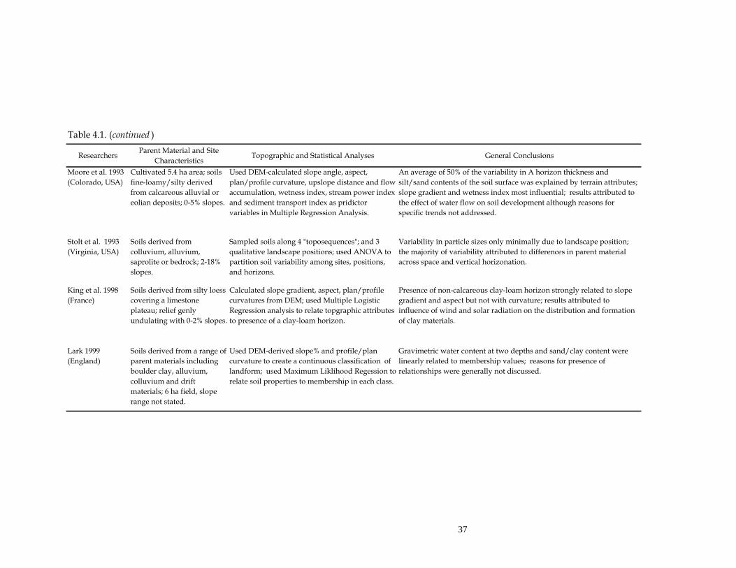
Table 4.1. (continued )
ResearchersParent Material and Site
CharacteristicsTopographic and Statistical Analyses General Conclusions
Moore et al. 1993
(Colorado, USA)
Cultivated 5.4 ha area; soils
fine-loamy/silty derived
from calcareous alluvial or
eolian deposits; 0-5% slopes.
Used DEM-calculated slope angle, aspect,
plan/profile curvature, upslope distance and flow
accumulation, wetness index, stream power index
and sediment transport index as pridictor
variables in Multiple Regression Analysis.
An average of 50% of the variability in A horizon thickness and
silt/sand contents of the soil surface was explained by terrain attributes;
slope gradient and wetness index most influential; results attributed to
the effect of water flow on soil development although reasons for
specific trends not addressed.
Stolt et al. 1993
(Virginia, USA)
Soils derived from
colluvium, alluvium,
saprolite or bedrock; 2-18%
slopes.
Sampled soils along 4 "toposequences"; and 3
qualitative landscape positions; used ANOVA to
partition soil variability among sites, positions,
and horizons.
Variability in particle sizes only minimally due to landscape position;
the majority of variability attributed to differences in parent material
across space and vertical horizonation.
King et al. 1998
(France)
Soils derived from silty loess
covering a limestone
plateau; relief genly
undulating with 0-2% slopes.
Calculated slope gradient, aspect, plan/profile
curvatures from DEM; used Multiple Logistic
Regression analysis to relate topgraphic attributes
to presence of a clay-loam horizon.
Presence of non-calcareous clay-loam horizon strongly related to slope
gradient and aspect but not with curvature; results attributed to
influence of wind and solar radiation on the distribution and formation
of clay materials.
Lark 1999
(England)
Soils derived from a range of
parent materials including
boulder clay, alluvium,
colluvium and drift
materials; 6 ha field, slope
range not stated.
Used DEM-derived slope% and profile/plan
curvature to create a continuous classification of
landform; used Maximum Liklihood Regession to
relate soil properties to membership in each class.
Gravimetric water content at two depths and sand/clay content were
linearly related to membership values; reasons for presence of
relationships were generally not discussed.

38
measurements taken in the field or from a DEM. Differences in measured soil
property mean values among topographic classes and within profiles in these
studies were often analysed using ANOVA procedures or, at times, by
descriptive analysis of soil types found. While this approach partitions
differences in soil characteristics among landscape zones, little direct
understanding is gained about the extent or direction of the relationships
between topography and soil properties.
Several of the cited studies (Walker et al. 1968; Moore et al. 1993; King et
al. 1998; Lark 1999) used regression techniques to relate terrain attributes or fuzzy
terrain classes to soil properties. This approach more adequately recognises the
continuous nature of soil property distributions, provides a quantitative means of
predicting spatial changes in these properties, and establishes a link between
water-flow and slope-mediated processes and soil patterns.
The dependence of soil development and physical properties on
topography, as illustrated by the reviewed studies, is highly variable. Walker et
al. (1968) and Moore et al. (1993) explained up to 60 % of the variation in certain
soil physical properties using topographic attributes while Stolt et al. (1993)
found that topography exerted only a minimal effect on soil properties at their
site. Nonetheless, slope shape, gradient, aspect, and flow accumulation were
clearly influential as landscape surrogates for the effect of surface and subsurface
water flow. For example, lateral water flow was explicitly stated as a substantial
influence on such characteristics as horizon thickness and texture by Dalsgaard et
39 39
al. (1981), Pennock et al. (1987), Donald et al. (1993) and Moore et al. (1993). The
degree of influence of water flow clearly depends on the combined effects of soil
parent material lithology and permeability, the complexity of topography (relief
and configuration), the degree of disturbance and local climate effects.
METHODS
Description of Sites, Sample Plots, and Field Methodologies
A detailed description of the two study sites and field methodologies used
in site selection, plot location and soil sampling were outlined in Chapter 2.
Laboratory and Statistical Methods
Soil samples were dried and subsequently sieved to remove coarse
fragments. Particle size distribution was examined using two different
approaches. Soil in each mineral horizon was first of all assessed for texture class
in the field using a series of finger assessment tests as outlined in Jones et al.
(1983), including moist cast, ribbon and various feel tests. As a comparison,
samples from each horizon at each plot were also analysed in the lab using the
hydrometer method (Day 1965) after dispersion, deflocculation and
sedimentation in a column.
The percentage of coarse fragments, horizon thickness and the effective
rooting depth were estimated in the field and were included here as dependent
variables in addition to soil texture fractions. Layer thickness, coarse fragments
40 40
and texture fractions were averaged for the “forest floor”, “A”, “B” and “subsoil
(SS)” layers as weighted by the depth of the horizons in each layer. Flow
accumulation, steady-state wetness index and slope % (see Chapter 3 for a
detailed explanation of their derivation) were used as topographic indices of
water flow and accumulation conditions at each plot. Scatter-plots of physical
property data and topographic attributes were initially examined to determine
the form of possible relationships. Flow accumulation generally displayed non-
linear relationships with soil properties and was subsequently log-transformed.
Subsequently, regression analyses were carried out to determine the degree of
correlation between topographic attributes and soil physical properties at each
site.
RESULTS AND DISCUSSION
Soil Texture Analysis
There were obvious discrepancies between the field test and hydrometer
methods (Table 4.2), particularly at the Island Lake site. Normally, an analysis of
particle size distribution yields results with an error of ±10 % (Indorante et al.
1990) . In this case, however, from 5 to 40 % of samples analysed using the
hydrometer method showed a consistent bias toward the sand fraction that was
obviously not evident in the field.
Measurement of these samples were likely confounded by a component
of fine coarse fragments that remained after sieving and because, for some
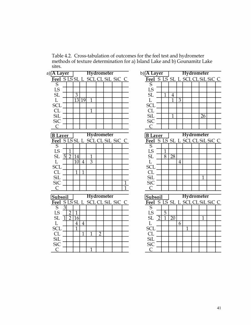
41 41
Table 4.2. Cross-tabulation of outcomes for the feel test and hydrometer methods of texture determination for a) Island Lake and b) Gounamitz Lake sites.
a) A Layer Hydrometer b) A Layer HydrometerFeel S LS SL L SCL CL SiL SiC C Feel S LS SL L SCL CL SiL SiC C
S SLS LSSL 3 SL 1 4L 13 19 1 L 1 3
SCL SCLCL 1 CLSiL SiL 1 26SiC SiCC C
B Layer Hydrometer B Layer HydrometerFeel S LS SL L SCL CL SiL SiC C Feel S LS SL L SCL CL SiL SiC C
S SLS 1 LS 1SL 5 2 14 1 SL 8 28L 10 4 3 L 4
SCL SCLCL 1 1 CLSiL SiL 1SiC 1 SiCC 1 C
Subsoil Hydrometer Subsoil HydrometerFeel S LS SL L SCL CL SiL SiC C Feel S LS SL L SCL CL SiL SiC C
S 3 SLS 2 1 LS 5SL 1 2 16 SL 2 1 20 1L 4 4 L 6
SCL 1 SCL 1CL 1 1 2 CLSiL SiLSiC SiCC 1 C
42 42
horizons, there was a less than adequate quantity of soil to provide a
representative sample. However, in samples where these problematic conditions
were absent, hydrometer-measured texture classes agreed closely with field
assessments, which were considered accurate since they were consistently
estimated by an experienced soil technician. Field-averaged textural classes were
deemed to be the more consistent standard in this study and were therefore used
to estimate sand, silt and clay fractions for samples where there was
disagreement between the two methods.
Overall Physical Property Variability
The most noticeable trend evident in physical properties (Table 4.3) is the
difference in both % coarse fragments and particle size distribution between the
two sites. Overall, the Gounamitz Lake site shows a significantly greater
percentage of silt in the A and subsoil layers and coarse fragments in the B and
subsoil layers. Conversely, the Island Lake site shows a higher average fraction
of clay in each mineral horizon, possibly due to the presence of finer-grained
rocks in the soil parent material. The range of % clay values is also much greater
at this site indicating a lateral flow and deposition of fine material from divergent
to convergent plots or, possibly, resulting from the action of freeze-thaw
processes.
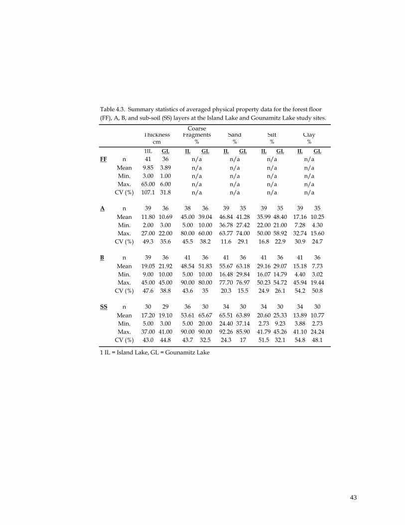
43 43
Table 4.3. Summary statistics of averaged physical property data for the forest floor
(FF), A, B, and sub-soil (SS) layers at the Island Lake and Gounamitz Lake study sites.
CoarseThickness Fragments Sand Silt Clay
cm % % % %
1IL GL IL GL IL GL IL GL IL GL
FF n 41 36 n/a n/a n/a n/a
Mean 9.85 3.89 n/a n/a n/a n/a
Min. 3.00 1.00 n/a n/a n/a n/a
Max. 65.00 6.00 n/a n/a n/a n/a
CV (%) 107.1 31.8 n/a n/a n/a n/a
A n 39 36 38 36 39 35 39 35 39 35
Mean 11.80 10.69 45.00 39.04 46.84 41.28 35.99 48.40 17.16 10.25
Min. 2.00 3.00 5.00 10.00 36.78 27.42 22.00 21.00 7.28 4.30
Max. 27.00 22.00 80.00 60.00 63.77 74.00 50.00 58.92 32.74 15.60
CV (%) 49.3 35.6 45.5 38.2 11.6 29.1 16.8 22.9 30.9 24.7
B n 39 36 41 36 41 36 41 36 41 36
Mean 19.05 21.92 48.54 51.83 55.67 63.18 29.16 29.07 15.18 7.73
Min. 9.00 10.00 5.00 10.00 16.48 29.84 16.07 14.79 4.40 3.02
Max. 45.00 45.00 90.00 80.00 77.70 76.97 50.23 54.72 45.94 19.44
CV (%) 47.6 38.8 43.6 35 20.3 15.5 24.9 26.1 54.2 50.8
SS n 30 29 36 30 34 30 34 30 34 30
Mean 17.20 19.10 53.61 65.67 65.51 63.89 20.60 25.33 13.89 10.77
Min. 5.00 3.00 5.00 20.00 24.40 37.14 2.73 9.23 3.88 2.73
Max. 37.00 41.00 90.00 90.00 92.26 85.90 41.79 45.26 41.10 24.24
CV (%) 43.0 44.8 43.7 32.5 24.3 17 51.5 32.1 54.8 48.1
1 IL = Island Lake, GL = Gounamitz Lake
44 44
Thickness of Soil Layers and Rooting Zone
Weak to moderate relationships existed between soil layer thickness and
topographic attributes with 22 % to 41 % and 19 % to 43 % of the variation
explained for the Island Lake (Figure 4.1) and Gounamitz Lake (Figure 4.2) sites
respectively. Furthermore, positive, linear trends existed at both sites between
effective rooting depth and slope gradient; relationships were moderately strong
with 31 % of the variation explained for this variable at Island Lake and 44 % at
the Gounamitz Lake site.
Forest Floor Thickness
The thickness of the forest floor, which ranged from thin (3 cm) to
relatively thick (20 cm) was positively related to the wetness index and slope
gradient at Island Lake (Figure 4.1a). Similar to Donald et al.’s (1993) findings at
a hummocky till site, these results reflected differences in decomposition among
slope positions; ridge areas (low flow accumulation and low slope gradient) were
dry and more exposed resulting in thin forest floors while footslope (high %
slope, moderate wetness) and depressional (high flow accumulation) areas were
generally wetter and accumulated a thick humus layer. At the Gounamitz site,
the range in forest floor thickness was small (1-6 cm), reflecting the fast turnover
of the tolerant hardwood litter. Even so, forest floor thickness was moderately
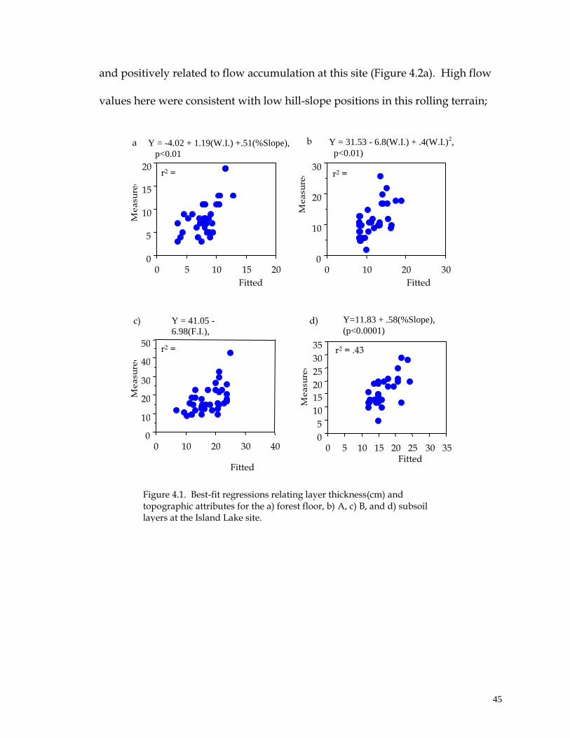
45 45
and positively related to flow accumulation at this site (Figure 4.2a). High flow
values here were consistent with low hill-slope positions in this rolling terrain;
Me
asu
red
0
10
20
30
0 10 20 30
Y = -4.02 + 1.19(W.I.) +.51(%Slope),
p<0.01
Y = 31.53 - 6.8(W.I.) + .4(W.I.)2,
p<0.01)
0
5
10
15
20
0 5 10 15 20
Y = 41.05 -
6.98(F.I.),
p<0.001
0
10
20
30
40
50
0 10 20 30 40
Y=11.83 + .58(%Slope),
(p<0.0001)
r2 = .34
r2 = .41
r2 = .37
a)
b)
c) d)
Figure 4.1. Best-fit regressions relating layer thickness(cm) and topographic attributes for the a) forest floor, b) A, c) B, and d) subsoil layers at the Island Lake site.
0
5
10
15
20
25
30
35
0 5 10 15 20 25 30 35
r2 = .43
Me
asu
red
Me
asu
red
Me
asu
red
Fitted
Fitted Fitted
Fitted
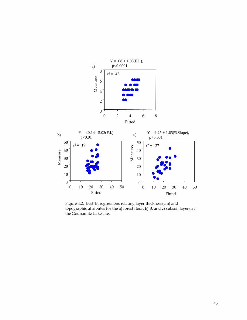
46 46
0
10
20
30
40
50
0 10 20 30 40 50
Y = .08 + 1.08(F.I.),
p<0.0001
0
2
4
6
8
0 2 4 6 8
Fitted
Y = 40.14 - 5.03(F.I.),
p<0.01
Y = 9.25 + 1.65(%Slope),
p<0.001
Fitted Fitted
r2 = .43
r2 = .19
Figure 4.2. Best-fit regressions relating layer thickness(cm) and topographic attributes for the a) forest floor, b) B, and c) subsoil layers.at the Gounamitz Lake site.
0
10
20
30
40
50
0 10 20 30 40 50
a)
b) c)
r2 = ..37
Me
asu
red
Me
asu
red
Me
asu
red
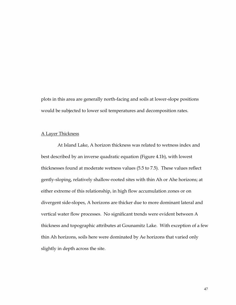
47 47
plots in this area are generally north-facing and soils at lower-slope positions
would be subjected to lower soil temperatures and decomposition rates.
A Layer Thickness
At Island Lake, A horizon thickness was related to wetness index and
best described by an inverse quadratic equation (Figure 4.1b), with lowest
thicknesses found at moderate wetness values (5.5 to 7.5). These values reflect
gently-sloping, relatively shallow-rooted sites with thin Ah or Ahe horizons; at
either extreme of this relationship, in high flow accumulation zones or on
divergent side-slopes, A horizons are thicker due to more dominant lateral and
vertical water flow processes. No significant trends were evident between A
thickness and topographic attributes at Gounamitz Lake. With exception of a few
thin Ah horizons, soils here were dominated by Ae horizons that varied only
slightly in depth across the site.

48 48
B Layer Thickness
B thickness was negatively related to flow accumulation at both sites
(Figure 4.1c). This trend was more pronounced at Island Lake, not surprisingly,
since this site is more heavily influenced by lateral water flow along constricted
subsoil layers and because these effects are most strongly reflected in the
development of the B horizon. In low flow zones, lateral and vertical through-
flow is strong and soils are deeper, resulting in well-developed illuvial B
horizons. Conversely, B horizons in high flow zones are generally imperfectly
drained, restricting soil development processes in these areas. At Gounamitz the
same relationship with flow accumulation existed but was substantially weaker
(Figure 4.2b); this site was consistently well-drained and dominant
eluvial/illuvial processes were probably more related to micro-scale variations in
vertical water flow, which may be greater in up-slope/hill-top areas where
gradients are more gentle overall.
Effective Rooting Depth and Subsoil Thickness
Rooting zone (Figure 4.3) and subsoil thickness were both positively and
moderately related to slope gradient at both sites. The depth of the effective
rooting zone reflects both heterogeneity of the glacial till parent material and the
influence of lateral water flow and accumulation. At Island Lake the latter
influence was more prominent, showing a decrease in rooting depth in
convergent areas where seepage water accumulates and restricts rooting, a
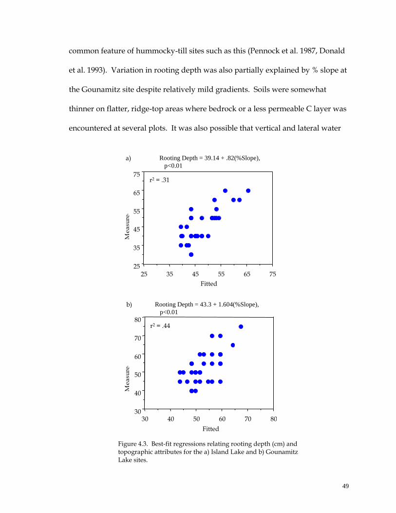
49 49
common feature of hummocky-till sites such as this (Pennock et al. 1987, Donald
et al. 1993). Variation in rooting depth was also partially explained by % slope at
the Gounamitz site despite relatively mild gradients. Soils were somewhat
thinner on flatter, ridge-top areas where bedrock or a less permeable C layer was
encountered at several plots. It was also possible that vertical and lateral water
25
35
45
55
65
75
25 35 45 55 65 75
Fitted
30
40
50
60
70
80
30 40 50 60 70 80
Fitted
Rooting Depth = 39.14 + .82(%Slope),
p<0.01
Rooting Depth = 43.3 + 1.604(%Slope),
p<0.01
r2 = .31
r2 = .44
Figure 4.3. Best-fit regressions relating rooting depth (cm) and topographic attributes for the a) Island Lake and b) Gounamitz Lake sites.
a)
b)
Me
asu
red
Me
asu
red
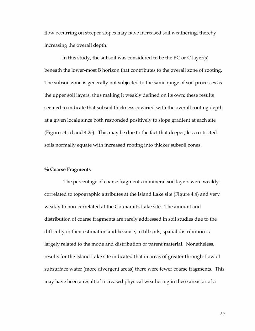
50 50
flow occurring on steeper slopes may have increased soil weathering, thereby
increasing the overall depth.
In this study, the subsoil was considered to be the BC or C layer(s)
beneath the lower-most B horizon that contributes to the overall zone of rooting.
The subsoil zone is generally not subjected to the same range of soil processes as
the upper soil layers, thus making it weakly defined on its own; these results
seemed to indicate that subsoil thickness covaried with the overall rooting depth
at a given locale since both responded positively to slope gradient at each site
(Figures 4.1d and 4.2c). This may be due to the fact that deeper, less restricted
soils normally equate with increased rooting into thicker subsoil zones.
% Coarse Fragments
The percentage of coarse fragments in mineral soil layers were weakly
correlated to topographic attributes at the Island Lake site (Figure 4.4) and very
weakly to non-correlated at the Gounamitz Lake site. The amount and
distribution of coarse fragments are rarely addressed in soil studies due to the
difficulty in their estimation and because, in till soils, spatial distribution is
largely related to the mode and distribution of parent material. Nonetheless,
results for the Island Lake site indicated that in areas of greater through-flow of
subsurface water (more divergent areas) there were fewer coarse fragments. This
may have been a result of increased physical weathering in these areas or of a
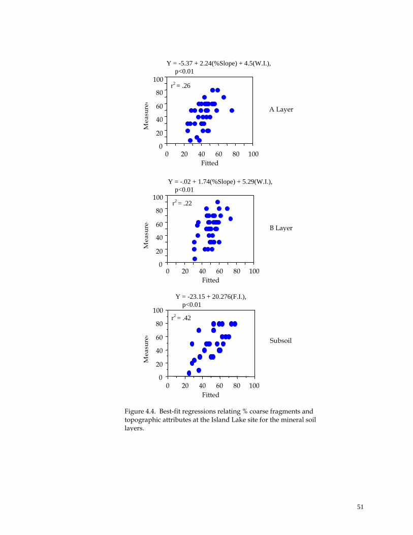
51 51
0
20
40
60
80
100
0 20 40 60 80 100
Fitted
Y = -5.37 + 2.24(%Slope) + 4.5(W.I.),
p<0.01
r2 = .26
Y = -.02 + 1.74(%Slope) + 5.29(W.I.),
p<0.01
0
20
40
60
80
100
0 20 40 60 80 100
Fitted
r2 = .22
0
20
40
60
80
100
0 20 40 60 80 100
Fitted
Y = -23.15 + 20.276(F.I.),
p<0.01
r2 = .42
Figure 4.4. Best-fit regressions relating % coarse fragments and topographic attributes at the Island Lake site for the mineral soil layers.
A Layer
B Layer
Subsoil
Me
asu
red
Me
asu
red
Me
asu
red
52 52
transport of material to convergent areas. I suggest that the former was probably
more likely since there was little evidence of significant erosional processes and
because igneous-derived materials would have responded to physical and
chemical weathering.
% Clay
Of the three particle size fractions examined, only the clay texture fraction
in the B and subsoil layers at the two sites were correlated with topographic
attributes (Figure 4.5). At Island Lake, clay was moderately and positively
related to flow accumulation (r2 = .41) in the B layer and more weakly and
negatively related to slope gradient (r2 = .30) in the subsoil. These findings
indicated that there was a possible enrichment of clay in convergent areas of
higher flow and where the slope gradient is milder at the bottom of slopes. Clay,
the finest texture fraction, is know to be fairly mobile; in areas of subsurface
water flow and moderate to strong slope gradients clay has been found to
accumulate in convergent areas (e.g. Odeh et al. 1993; Brubaker et al. 1993;
Donald et al. 1993). This is logical at this site where there were shorter, steeper
slopes lead to many convergent depressional areas and where subsurface flow
occurs along more compact B and subsoil layers. Secondly, mildly sloping areas
appeared to have thinner, moister soils promoting freeze and thaw processes and
the weathering of volcanic rocks such as basalt and tuff into clay-sized fractions.
53 53
b)
Fitted
0
10
20
30
40
0 10 20 30
40
Y = -5.72 + 5.83(F.I.),
p<0.0001
a)
r2 = .41 B Layer
Y = -9.4 + 2.16(W.I.)+ .79(%Slope),
p<0.0001
0 10 20 30 0
10
20
30 r2 = .50
Subsoil
0
5
10
15
20
25
0 5 10 15 20 25
Y = -4.15 + 3.37(F.I.),
p<0.001 r2 = ..33 B Layer
Fitted
Figure 4.5. Best-fit regressions relating % clay and topographic attributes at the a) Island Lake and b) Gounamitz Lake site for the B and Subsoil layers. Bracketed points were removed from the analysis.
Y = 15.92 - .45(%Slope),
p<0.001 r2 = .30
0
10
20
30
40
50
0 10 20 30 40 50
[ ]
[ ]
Fitted
Fitted
Me
asu
red
Me
asu
red
Me
asu
red
Me
asu
red
54 54
Although similar relationships were evident at the Gounamitz site, it is less likely
that clay would accumulate due to water flow since slopes are gentler and the
degree of convergence is subtler. I suspect that the increase in the
clay fraction with increasing flow accumulation and wetness index reflected the
increase in weathering of siltstone and shale in areas receiving relatively more
water flow and moisture, laterally and vertically.
SUMMARY
As commonly concluded in studies relating physical soil properties to
topography, there was still much variation unexplained in distributions of the
physical characteristics investigated here. Few studies using analyses similar to
those used here explained more than 50% of the variation in physical properties.
The amount of topographic influence suggested by these results were not
surprising for soils derived from basal till parent material; the depth and
composition of glacially-deposited materials are known to be highly spatially
heterogeneous and therefore difficult to predict.
Although relationships were weak, there were significant correlations
between topographic attributes and layer and rooting thickness, % coarse
fragments and % clay across horizons and between sites. Further, and more
importantly, most physical variables appeared to be influenced in a similar

55 55
manner and by the same topographic attributes at both sites. These results
therefore suggest that water flow and accumulation have had a measure of
influence on soil physical properties at these sub-catchments despite site-specific
differences in topographic complexity and substrate permeability. Stronger
results may be evident with a more quantitative measurement of these and other
soil physical properties and with an increase in accuracy of topographic attribute
derivation, especially in areas of subtle topography.

56 56
CHAPTER 5
THE INFLUENCE OF WATER FLOW AND ACCUMULATION AND PARENT
MATERIAL ON SOIL CHEMICAL DISTRIBUTIONS
INTRODUCTION
Like physical soil characteristics, spatial distributions of soil-chemical
properties are often highly variable in time and space (Hammer et al. 1987). Soil
chemistry is influenced by both the physical composition of soil (e.g. soil texture,
structure, coarse fragments) at a given location and factors such as local water
flow and accumulation and soil temperatures which change throughout the year.
At a meso-scale (defined here as distances of 10-100 m), in areas of relatively
consistent geology, climate and vegetation, water flow and accumulation in the
landscape has been recognised as a dominant driving-mechanism for many soil-
related processes (Moore et al. 1991) and therefore contributes to overall spatial
variability in soil chemical properties.
Various measures of landform shape and configuration, due to their
influence on near-surface and surface hydrology, have proved to be useful
predictors of the distribution of soil chemical and physical properties at the local
topographic scale. Some researchers have divided study areas into qualitative
terrain classes or landscape positions, striving to isolate catenary slope processes;
significant differences in chemical soil properties were found at a range of sites as
influenced by slope and aspect class (e.g. King et al. 1983; Carter and Ciolkosz
57 57
1991; Hairston and Grigal 1991; Odeh et al. 1991) and landscape position (e.g.
Kreznor et al. 1989; Raghubanshi 1992; Brubaker et al. 1993; Silver et al. 1994;
Osher and Buol 1998). Qualitative slope units, however, are simplistic two-
dimensional classifications of landform and do not provide a consistent,
quantitative measure of specific topographic attributes (Moore et al. 1993).
It has long been recognised by soil-landscape researchers that landscape
paradigms characterising the landscape in three dimensions can more accurately
address soil formation and chemical distribution since water flow and
accumulation, as well as the distribution of energy, are complex three-
dimensional phenomena (e.g. Jenny 1941, Aandahl 1948; Walker et al. 1968;
Hugget 1975; Connacher and Dalrymple 1977, O’Loughlin 1986). Several studies
carried out at a meso-scale have shown soil properties to be related to
topographic attributes. Donald et al. (1993) found variations in certain soil
physical properties and pH were largely explained by plan/profile convexity and
slope gradient; Odeh et al. (1991) and Moore et al. (1993) showed that these same
topographic indices, as well as flow accumulation and wetness index, were
linearly related to soil properties. Each of the studies concluded that spatial
distribution of soil properties observed were largely the result of a re-distribution
of soil materials due to lateral water flow from divergent to convergent zones.
Morris and Boerner (1998) found N mineralization and nitrification,
organic C and pH to be highly related to an integrated moisture index , calculated
using a combination of various DEM-derived attributes, including flow

58 58
accumulation. They concluded that many bio-physical processes operating at a
meso-scale are dependent on local topography and its influence on soil moisture
status.
In this chapter, I address two questions in comparing the two landscape
types characterised by the Island Lake and Gounamitz Lake sites: (1) to what
degree do derived indices of water flow and accumulation explain spatial trends
in soil chemical properties in each soil layer? and; (2) since soil chemistry, at a
fine scale, is usually also dependent on parent material factors, what is the
additional influence of site-specific properties such as texture, coarse fragment
abundance, and rooting depth in predicting soil chemical distributions?
METHODS
Description of Study Sites, Sample Plots, and Field Methodologies
A detailed description of the study sites and field methodologies used in
site selection, plot location, and soil sampling were outlined in Chapter 2.
Soil Sample Preparation and Laboratory Analysis
Total nitrogen, total carbon, pH, exchangeable cations, and extractable
phosphorous were measured for samples from all soil horizons described at each
plot. Texture fractions were determined as outlined in Chapter 4.
Slurries made with 1:3 ratio of fresh soil and 0.01M CaCl2 were analysed
for pH using a digital pH meter. Samples were then dried at 70°C for 72 hours,
59 59
ground with a mortar and pestle and passed through a 2 mm sieve to remove
coarse fragments; dried samples were used for the remaining analyses.
Total nitrogen was measured via Kjeldahl digestion, steam distillation
and analysis with a Buchi/Brinkmann nitrogen system. Total carbon was
measured by dry combustion in a LECO EC-12 Induction Furnace. Exchangeable
cations were extracted by shaking soils in 1M NH4Cl for 30 minutes followed by
suction filtering through Whatman 41 filter paper. A Varian Spectra atomic
absorption spectrophotometer was used to analyse extracts for exchangeable
cations, Al, Fe and Mn. Phosphorous was extracted using the bicarbonate
method and measured colorimetrically, after pH adjustment using the ascorbic
acid-molybdenum blue procedure (Murphy and Riley 1962), with an LKB
Ultraspec 4050 spectrophotometer.
Topographic and Statistical Analyses
Expected values for flow accumulation, wetness index were derived as
discussed in Chapter 3. Physical soil data, element concentrations and selected
site variables were averaged for each soil horizon within the forest floor, A, B and
subsoil, weighted by horizon depth. Descriptive statistics were generated to
provide a comparison of the overall soil property variability for data averaged
across plots at each project site. Most soil chemicals appeared to have positively-
skewed frequencies (see Table 5.1), showed heteroscedasticity and were
subsequently log-transformed using the equation: log(Y * 10,000), where Y is the
60 60
chemical concentration multiplied by 10,000, to code low concentration values as
a set of final values ranging between 0 and 10 for graphing purposes (Sokal and
Rohlf 1981, p. 421). Scatter plots were used to analyse trends between layer-
specific soil chemical and physical data and topographic variables. Simple linear
regressions were used initially to determine the amount of variability in soil
chemistry explained by expected flow accumulation alone; subsequently, other
topographic and physical soil variables were added into a multiple regression to
determine their contribution to the overall variation at each project site.
RESULTS AND DISCUSSION
Soil Variability
In an aspatial context, a substantial degree of variability existed in soil
chemical properties at both project sites (Table 5.1). Overall, the coefficient of
variation was the lowest for pH, while available Ca, Mg, Fe, Al and P all showed
high CV’s, mainly because mean values for these elements were low in
comparison to a high total variance. This high range of variation and skewness is
not uncommon with soil nutrient data (Young et al. 1999) and may have reflected
the focus of sampling both perceived flow accumulation zones and up-slope
ridge zones or was due to inherent heterogeneity in the glacial till parent
material.
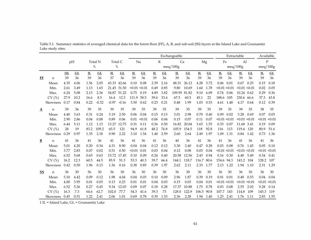
61
Table 5.1. Summary statistics of averaged chemical data for the forest floor (FF), A, B, and sub-soil (SS) layers at the Island Lake and Gounamitz
Lake study sites.
Exchangeable Extractable Available
pH Total N Total C Na K Ca Mg Fe Al P
% % meq/100g meq/100g meq/100g
1IL GL IL GL IL GL IL GL IL GL IL GL IL GL IL GL IL GL IL GL
FF n 39 36 39 36 37 36 39 36 39 36 39 36 39 36 39 36 39 36 39 36
Mean 4.35 4.06 1.56 2.05 43.33 42.66 0.10 0.08 2.39 2.16 48.31 26.12 4.28 3.72 0.06 0.01 0.67 0.25 0.15 0.18
Min. 2.61 3.49 1.13 1.65 21.45 31.50 <0.01 <0.01 0.49 0.85 9.80 10.69 1.60 1.78 <0.01 <0.01 <0.01 <0.01 0.02 0.05
Max. 6.24 5.08 2.13 2.36 54.87 51.22 0.75 0.19 4.89 3.82 109.95 81.82 9.10 6.09 0.74 0.06 10.24 0.62 0.29 0.36
CV (%) 27.9 10.2 16.6 8.5 16.4 12.3 111.9 58.5 39.6 33.4 67.5 60.5 45.1 22 188.6 105 230.6 66.6 37.3 43.8
Skewness 0.17 0.84 0.22 -0.32 -0.97 -0.16 3.50 0.62 0.23 0.21 0.48 1.99 1.03 0.53 4.61 1.48 4.17 0.64 0.12 0.39
A n 39 36 39 35 39 35 39 35 39 35 39 35 39 35 39 35 39 35 38 35
Mean 4.40 3.63 0.31 0.24 5.19 2.50 0.06 0.04 0.15 0.13 3.01 2.98 0.70 0.40 0.09 0.02 3.28 0.69 0.07 0.03
Min. 2.90 2.86 0.04 0.08 0.89 0.06 0.01 <0.01 0.06 0.04 0.15 0.07 0.11 0.07 <0.01 <0.01 <0.01 <0.01 <0.01 <0.01
Max. 6.44 5.11 1.12 1.13 13.27 12.75 0.31 0.11 0.36 0.50 16.82 20.04 3.65 1.55 0.35 0.07 11.68 3.41 0.19 0.09
CV (%) 28 19 83.2 109.2 65.5 121 94.9 61.8 48.2 76.8 105.9 154.5 118 92.8 116 113 119.4 120 80.9 51.6
Skewness 0.29 0.97 1.35 2.18 0.90 2.22 3.10 1.54 1.40 2.59 2.60 2.64 2.49 1.97 1.09 1.31 0.84 1.42 0.73 1.36
B n 41 36 41 36 41 36 41 36 41 36 40 36 41 36 41 36 41 36 41 36
Mean 5.01 4.20 0.20 0.34 4.31 8.90 0.04 0.04 0.12 0.12 3.30 2.40 0.47 0.28 0.03 0.08 0.76 1.45 0.05 0.10
Min. 3.77 2.83 0.07 0.02 0.51 0.50 <0.01 0.01 0.03 0.04 0.12 0.08 0.03 0.04 <0.01 <0.01 <0.01 <0.01 <0.01 <0.01
Max. 6.52 5.68 0.65 0.63 15.72 17.45 0.10 0.09 0.24 0.40 20.58 12.56 2.45 0.94 0.16 0.30 4.48 5.49 0.34 0.41
CV (%) 16.2 12.3 60.5 44.5 85.9 51.3 53.3 40.3 39.7 66.4 144.1 118.7 116.7 80.6 154.6 94.3 143.2 104 128.2 107
Skewness 0.42 0.50 1.96 0.13 1.36 0.16 0.38 0.85 0.39 1.97 2.62 2.11 2.33 1.77 2.13 1.22 1.94 1.10 2.31 1.29
SS n 36 30 36 30 36 30 36 30 36 30 36 30 36 30 36 30 36 30 36 30
Mean 5.10 4.42 0.09 0.12 1.98 4.04 0.04 0.03 0.10 0.09 2.96 1.87 0.39 0.19 0.01 0.01 0.48 0.53 0.04 0.04
Min. 4.00 3.95 0.01 0.03 0.13 0.23 0.01 0.01 0.04 0.03 0.15 0.03 0.04 0.01 <0.01 <0.01 <0.01 <0.01 <0.01 <0.01
Max. 6.52 5.26 0.27 0.45 9.34 12.03 0.09 0.07 0.18 0.28 17.37 10.88 1.75 0.78 0.03 0.08 2.55 2.02 0.28 0.14
CV (%) 16.3 7.3 64.6 62.7 102.0 77.7 54.3 41.6 39.3 73 128.0 122.9 106.5 90.8 107.7 143 114.8 109 145.3 119
Skewness 0.45 0.51 1.22 2.41 2.06 1.01 0.69 0.78 0.39 1.53 2.36 2.28 1.94 1.40 1.23 2.41 1.76 1.11 2.83 1.55
1 IL = Island Lake, GL = Gounamitz Lake
62
Trends in variation were similar for most soil chemicals at both sites
within soil horizons, although the Island Lake site displayed a greater range of
variation. Similar trends existed in mean values between sites and among soil
horizons. All soil chemical concentrations and acidity generally decreased
vertically through the profiles; the Gounamitz Lake site, however, showed higher
values of Fe, Al and organic matter within the B horizon, due to dominant
eluvial/illuvial processes occurring across this site. Additionally, pH at the
Gounamitz Lake site was surprisingly lower on average than at Island Lake’s,
suggesting that the surface geology is probably comprised mainly of sand and
siltstones of low calcium content, contrary to soil map classifications.
Influence of Flow Accumulation on Soil Chemistry
Effects of water flow, either laterally, vertically or both, on the variability
soil properties examined is clearly evident at both sites to varying degrees.
Chemical concentration trends were log-linear with flow accumulation (Figure
5.1), with the greatest rate of change in soil chemicals occurring at flow
accumulation values between 500 and 15,000 m2, where there is a maximum
transition from steeper divergent zones to convergent areas and the greatest
effect from direct lateral flow. Much stronger relationships between soil
chemistry and flow accumulation were evident at the Island Lake site as
compared to the Gounamitz Lake (Table 5.2) site although both sites show similar
directional trends (Figure 5.1).
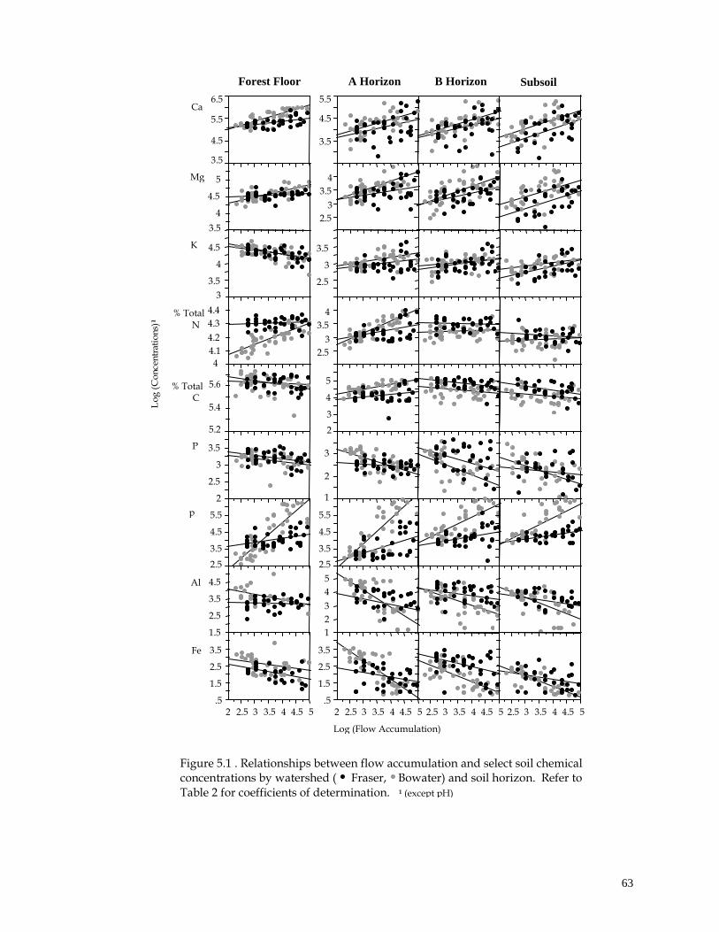
63 63
Forest Floor A Horizon B Horizon Subsoil
Figure 5.1 . Relationships between flow accumulation and select soil chemical concentrations by watershed ( Fraser, Bowater) and soil horizon. Refer to Table 2 for coefficients of determination. 1 (except pH)
2.5 3
3.5 4
3.5 4.5 5.5
2.5 3
3.5
2.5 3
3.5 4
2 3 4 5
1 2 3
2.5 3.5 4.5 5.5
1 2 3 4 5
2 2.5 3 3.5 4 4.5 5 .5 1.5 2.5 3.5
2.5 3 3.5 4 4.5 5 2.5 3 3.5 4 4.5 5
Mg
3.5 4
4.5 5
Ca
3.5 4.5 5.5 6.5
3 3.5
4 4.5 K
% Total N
4 4.1 4.2 4.3 4.4
5.2 5.4 5.6
P
2 2.5
3 3.5
pH
2.5 3.5 4.5 5.5
1.5 2.5 3.5 4.5 Al
2 2.5 3 3.5 4 4.5 5 .5 1.5 2.5 3.5
% Total C
Fe
Log (Flow Accumulation)
Lo
g (
Co
nce
ntr
atio
ns)
1
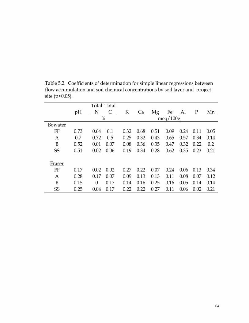
64 64
Table 5.2. Coefficients of determination for simple linear regressions between flow accumulation and soil chemical concentrations by soil layer and projectsite (p<0.05).
Total TotalpH N C K Ca Mg Fe Al P Mn
% meq/100gBowater
FF 0.73 0.64 0.1 0.32 0.68 0.51 0.09 0.24 0.11 0.05A 0.7 0.72 0.5 0.25 0.32 0.43 0.65 0.57 0.34 0.14B 0.52 0.01 0.07 0.08 0.36 0.35 0.47 0.32 0.22 0.2SS 0.51 0.02 0.06 0.19 0.34 0.28 0.62 0.35 0.23 0.21
FraserFF 0.17 0.02 0.02 0.27 0.22 0.07 0.24 0.06 0.13 0.34A 0.28 0.17 0.07 0.09 0.13 0.13 0.11 0.08 0.07 0.12B 0.15 0 0.17 0.14 0.16 0.25 0.16 0.05 0.14 0.14SS 0.25 0.04 0.17 0.22 0.22 0.27 0.11 0.06 0.02 0.21
65 65
Exchangeable cations, pH, and % N all displayed positive correlation
with flow accumulation, while % C (except the A horizon), Al, Fe, and P showed
negative relationships. As a whole, Ca, Mg, and pH were most highly correlated
to flow accumulation at both sites, while Al, Fe, % N, % C and P were also
significantly correlated at the Island Lake site. Flow accumulation explained
from 10 to 73% of the variation in soil chemistry in the surface soil layers (FF and
A) at Island Lake’s, while moderate correlations were also evident at this site in
the B and subsoil layers for pH, Ca, Mg, Al, Fe, and P with coefficients of
determination ranging from 22 to 62%. In comparison, only <1 to 28 % of the
variation in soil chemistry was explained by flow accumulation for the
Gounamitz Lake site as a whole.
Assuming that the relative flow accumulation situation at each plot
location was reasonably estimated using available DEM and field accounts,
differences in correlation strength between project sites are most likely due to the
permeability of the soil and bedrock at each site. The widespread presence of
well-developed eluviated A horizons, a high coarse fragment content and
underlying sandstone bedrock at the Gounamitz Lake site suggested that a large
proportion of flood or melt-water infiltrated vertically through the profile to
lower horizons, travelled laterally in the subsoil or left as deep seepage. Water at
the Island Lake site, by contrast, appeared to flow laterally in many areas, either

66 66
as seepage along compact/cemented subsoil horizons or eventually as ground-
water, which came close to the surface in lower lying areas.
Although observed trends with flow accumulation were weaker at the
Gounamitz Lake site, it is certainly noteworthy that there was a consensus in
directional trends at both sites for all horizons and soil chemicals, suggesting that
processes controlling soil chemical distribution respond to water flow and
accumulation in a similar manner, even in such contrasting landscapes. This
makes sense since the action of water flow is universal; it is how and where water
flows (as influenced by topography and substrate) that determines the degree of
influence.
Highest correlations were found for Ca, Mg and pH , which increased
from areas of high flow accumulation to areas of low accumulation. The decrease
in acidity down-slope has been observed in other studies (Donald et al. 1993;
Moore et al. 1993; Silver et al. 1994) and is logically positively related to the lateral
seepage of base-rich water to down-slope, convergent positions. Fe and Al , on
the other hand, decreased with increasing flow accumulation and were strongly
and negatively correlated with pH (Appendix I) and flow accumulation at both
sites and for all layers. At the Island Lake site in particular, it appears that these
elements occur in higher concentrations in ridge areas, decreasing along well-
drained, steeper slopes and finally levelling off in convergent areas where flow
accumulation values are greater than 10 000 m2. In acidic forest soils,
exchangeable Al and pH are inversely related (Brady 1990; Appendix I), while

67 67
exchangeable Fe is higher in dry areas where it is present as Fe3+, becoming
reduced in seepage areas or where drainage is impeded (Silver et al. 1994).
Available phosphorous was also negatively, though weakly, correlated
with flow accumulation; P is present in low concentrations at both sites and is
notoriously difficult to quantify in a spatial context since its availability is
dependent largely on mineral weathering and because it is quickly immobilised
in acidic soils (Silver et al. 1994, Brady 1990). Similarly, % C, with the exception
of the A horizon, shows a negative correlation with flow accumulation, though I
would have expected it to be greater in convergent, high flow accumulation
zones where organic matter normally accumulates from lateral transport and due
to anaerobic conditions; % C, however, was also weakly related to flow
accumulation indicating that this particular topographic attribute may not be a
driving mechanism for organic matter distribution. High flow accumulation,
especially at Gounamitz, does not necessarily equate directly with long-term
moisture, shown to be important to carbon distribution in other studies (Pennock
and van Kessel 1997; Arrouays et al. 1998; Morris and Boerner 1998) and probably
a limiting factor at this site.
The Added Influence of Parent Material
Significant improvements in the prediction of mineral layer chemical
concentrations at both sites were achieved with multiple regression analysis
(Tables 5.3 and 5.4) as compared to simple regressions with flow accumulation
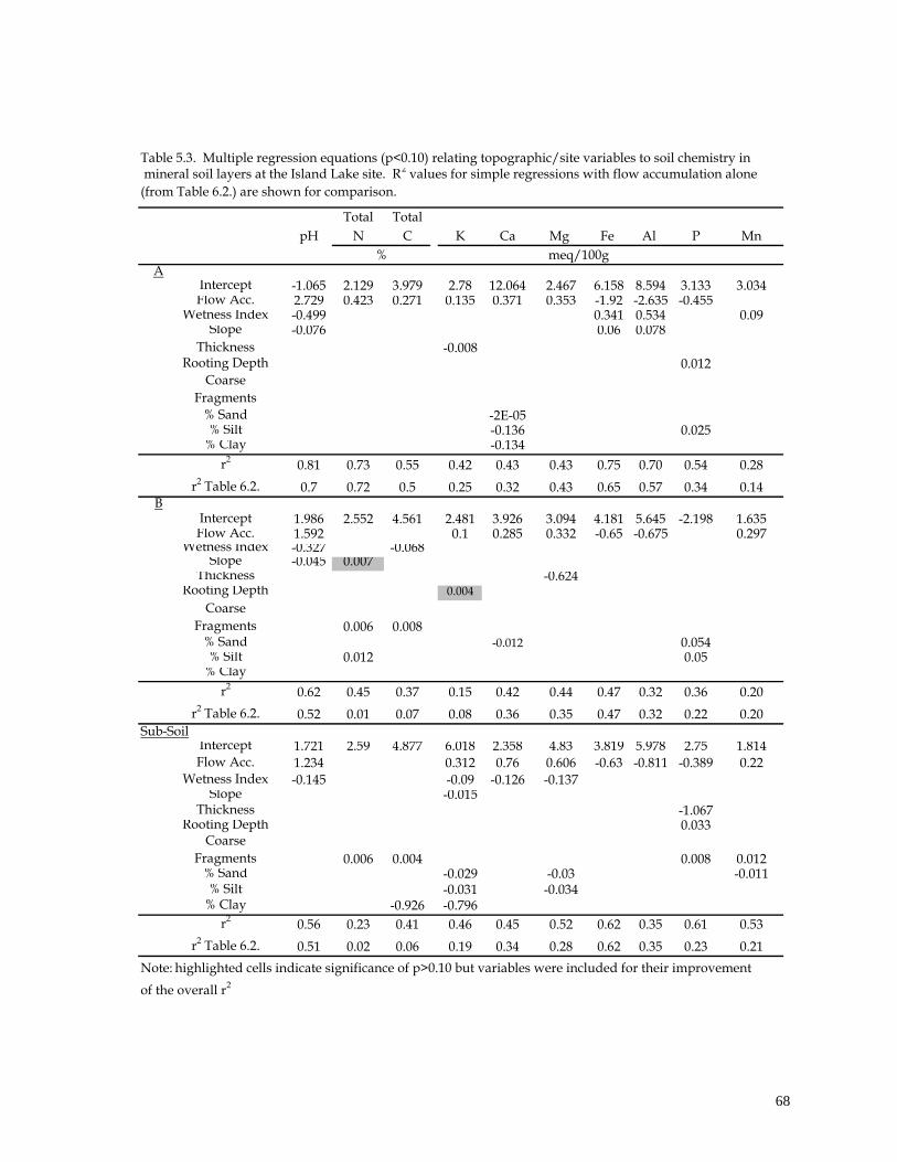
68 68
Table 5.3. Multiple regression equations (p<0.10) relating topographic/site variables to soil chemistry in mineral soil layers at the Island Lake site. R2 values for simple regressions with flow accumulation alone
(from Table 6.2.) are shown for comparison.
Total Total
pH N C K Ca Mg Fe Al P Mn
AIntercept -1.065 2.129 3.979 2.78 12.064 2.467 6.158 8.594 3.133 3.034Flow Acc. 2.729 0.423 0.271 0.135 0.371 0.353 -1.92 -2.635 -0.455
Wetness Index -0.499 0.341 0.534 0.09Slope -0.076 0.06 0.078
Thickness -0.008Rooting Depth 0.012
Coarse
Fragments
% Sand -2E-05% Silt -0.136 0.025
% Clay -0.134
r20.81 0.73 0.55 0.42 0.43 0.43 0.75 0.70 0.54 0.28
r2 Table 6.2. 0.7 0.72 0.5 0.25 0.32 0.43 0.65 0.57 0.34 0.14B
Intercept 1.986 2.552 4.561 2.481 3.926 3.094 4.181 5.645 -2.198 1.635Flow Acc. 1.592 0.1 0.285 0.332 -0.65 -0.675 0.297
Wetness Index -0.327 -0.068Slope -0.045 0.007
Thickness -0.624Rooting Depth 0.004
Coarse
Fragments 0.006 0.008% Sand -0.012 0.054% Silt 0.012 0.05
% Clay
r20.62 0.45 0.37 0.15 0.42 0.44 0.47 0.32 0.36 0.20
r2 Table 6.2. 0.52 0.01 0.07 0.08 0.36 0.35 0.47 0.32 0.22 0.20
Sub-SoilIntercept 1.721 2.59 4.877 6.018 2.358 4.83 3.819 5.978 2.75 1.814Flow Acc. 1.234 0.312 0.76 0.606 -0.63 -0.811 -0.389 0.22
Wetness Index -0.145 -0.09 -0.126 -0.137Slope -0.015
Thickness -1.067Rooting Depth 0.033
Coarse
Fragments 0.006 0.004 0.008 0.012% Sand -0.029 -0.03 -0.011% Silt -0.031 -0.034
% Clay -0.926 -0.796
r20.56 0.23 0.41 0.46 0.45 0.52 0.62 0.35 0.61 0.53
r2 Table 6.2. 0.51 0.02 0.06 0.19 0.34 0.28 0.62 0.35 0.23 0.21
Note: highlighted cells indicate significance of p>0.10 but variables were included for their improvement
of the overall r2
% meq/100g
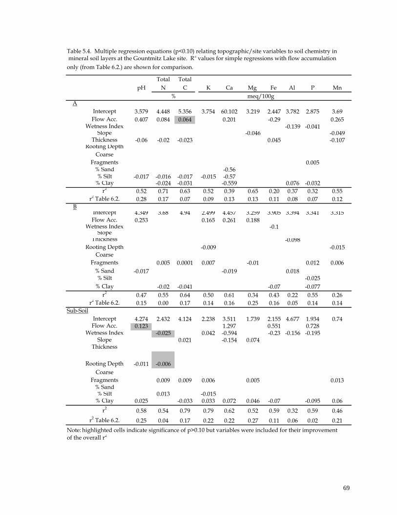
69 69
Table 5.4. Multiple regression equations (p<0.10) relating topographic/site variables to soil chemistry in mineral soil layers at the Gountmitz Lake site. R2 values for simple regressions with flow accumulation
only (from Table 6.2.) are shown for comparison.
Total Total
pH N C K Ca Mg Fe Al P Mn
A
Intercept 3.579 4.448 5.356 3.754 60.102 3.219 2.447 3.782 2.875 3.69
Flow Acc. 0.407 0.084 0.064 0.201 -0.29 0.265Wetness Index -0.139 -0.041
Slope -0.046 -0.049Thickness -0.06 -0.02 -0.023 0.045 -0.107
Rooting Depth
Coarse
Fragments 0.005% Sand -0.56% Silt -0.017 -0.016 -0.017 -0.015 -0.57
% Clay -0.024 -0.031 -0.559 0.076 -0.032
r20.52 0.71 0.63 0.52 0.39 0.65 0.20 0.37 0.32 0.55
r2 Table 6.2. 0.28 0.17 0.07 0.09 0.13 0.13 0.11 0.08 0.07 0.12
BIntercept 4.349 3.68 4.94 2.499 4.457 3.259 3.905 3.394 3.341 3.315Flow Acc. 0.253 0.165 0.261 0.188
Wetness Index -0.1Slope
Thickness -0.098Rooting Depth -0.009 -0.015
Coarse
Fragments 0.005 0.0001 0.007 -0.01 0.012 0.006
% Sand -0.017 -0.019 0.018% Silt -0.025
% Clay -0.02 -0.041 -0.07 -0.077
r20.47 0.55 0.64 0.50 0.61 0.34 0.43 0.22 0.55 0.26
r2 Table 6.2. 0.15 0.00 0.17 0.14 0.16 0.25 0.16 0.05 0.14 0.14
Sub-Soil
Intercept 4.274 2.432 4.124 2.238 3.511 1.739 2.155 4.677 1.934 0.74Flow Acc. 0.123 1.297 0.551 0.728
Wetness Index -0.025 0.042 -0.594 -0.23 -0.156 -0.195Slope 0.021 -0.154 0.074
Thickness
Rooting Depth -0.011 -0.006
Coarse
Fragments 0.009 0.009 0.006 0.005 0.013% Sand% Silt 0.013 -0.015
% Clay 0.025 -0.033 0.033 0.072 0.046 -0.07 -0.095 0.06
r20.58 0.54 0.79 0.79 0.62 0.52 0.59 0.32 0.59 0.46
r2 Table 6.2. 0.25 0.04 0.17 0.22 0.22 0.27 0.11 0.06 0.02 0.21
Note: highlighted cells indicate significance of p>0.10 but variables were included for their improvement
of the overall r2
% meq/100g
70 70
alone (Table 5.2). Indeed, flow accumulation was statistically non-significant for
several soil chemicals on the Gounamitz Lake site, although the effect of texture
and coarse fragments was fairly wide-spread and considerable. Conversely, flow
accumulation remained the dominant predictor at the Island Lake site, with
wetness index, slope and aspect all adding significant components to the
equations; these topographic parameters were important in the subsoil layer at
Gounamitz Lake as well. Overall, 20 – 70 %, 22 – 64 % and 32 – 79 % of the
variation in acidity and soil chemical concentrations at Gounamitz Lake could be
explained for the A, B and subsoil horizons respectively with the addition of
multiple factors, while 28 – 81 %, 20 – 62 % and 23 – 62 % of the variation was
explained at Island Lake’s for the same soil layers.
Multiple regression results at the Gounamitz Lake site were complex and
somewhat unexpected, probably due to the influence of strong micro-scale
eluvial/illuvial processes dominating the A and B layers across the area. For
example, % silt and % clay were negatively related to various soil chemicals in
these layers while coarse fragments were positively related to most chemicals in
the B and subsoil layers. Differences in texture here co-varied significantly with
soil acidity and reflected micro-scale variations in weathering of sandstone and
siltstone parent materials. Soil development responded to spatial changes in pH
(ranging from 5.6 to 3.5) across the site, varying from dystric brunisolic (most
basic) to orthic ferro-humic podzol and orthic humo-ferric (most acidic). Subtle
differences in acidity and soil development processes were possibly the

71 71
mediating influence on soil chemistry at the Gounamitz site. Although the direct
relationship of these factors to the mechanisms of nutrient distribution are
somewhat unclear here, predictions were nonetheless improved by the inclusion
of soil physical properties, due to their combined influence on acidity, aeration
and soil structure in these horizons.
Flow accumulation remained most significant at the Island Lake site, re-
iterating the influence of lateral water flow and moisture distribution in this
hummocky, relatively impermeable landscape. Soil physical properties generally
did not contribute much more to predictions than flow accumulation alone,
although the inclusion of slope and wetness index led to slight improvements. I
suspect that predictions would be improved at this site by increasing the
resolution and precision of topographic indices describing landform morphology
and spatial and temporal patterns of subsoil water flow.
Most noticeable at both sites was the improvement in % C and % N with
the inclusion of physical variables. Areas of increasing flow accumulation
positively influenced the presence of these components in the A horizon at both
sites but was not a statistically significant factor in the B or subsoil layers.
Organic matter distribution in these horizons was probably most related to the
decomposition of fine roots as influenced by soil aeration factors and soil acidity.
Correlation among soil chemicals showed % C to be strongly correlated with the
presence of % N, and moderately related to P and base cation concentration at
both sites (see Appendix I), suggesting that organic matter plays a key role in the

72 72
availability of nitrogen and the adsorption of other nutrients. The role of organic
matter in lower mineral soil layers is frequently not included in soil nutrient
studies though these horizons may, in certain regions, contain more organic
carbon than surface layers (Hammer et al. 1995). Predictions of P, K and base-
cation concentrations, at the Gounamitz Lake site in particular, were also much
improved by the inclusion of soil physical factors for their effect on supply and
retention of these nutrients. Moore et al. (1993) stated that it would be
unreasonable to expect more than 70 % of the variance in soil properties to be
explained, even with accurate depiction of micro-scale topography. I, therefore,
consider the amount of soil chemical variability explained at both sites in this
study to be significant and encouraging.
SUMMARY
Knowledge of the scales at which various soil processes controlling
available supplies of nutrients operate is extremely valuable in various aspects of
forest ecology, yet this cross-scale knowledge is rarely readily available and
difficult to obtain (Moore et al. 1993; Hammer 1998). In this study, supporting the
findings of other similar investigations, I presented strong evidence that
topography provides a crucial link between soil processes (as influenced by water
flow and accumulation) and spatial patterns of soil chemical properties at a meso-
scale. This study also further suggests that these relationships may be similar in
form for different soil-landscapes and that the strength of this linkage is related to

73 73
substrate permeability and its influence on overland and subsurface water flow
patterns. Therefore, the degree to which a given landscape is made up of
repeating topographic patterns and identifiable substrates may determine to
what extent results such as these can be scaled up. Watershed sub-catchments
are ideal for this purpose since they are basic, nested hydrological units that can
be automatically delineated and related to other GIS coverages.
Similar to Hairston and Grigal’s (1991) study findings, soil nutrients were
highly variable at sites in this study even though they lie within single soil-map
units; certain soil processes, especially those controlling fine-scale soil nutrient
availability, were localised to each landscape type and variably dependent on
both lateral water movement and vertical parent material composition within a
profile. Therefore, depending on the nature of the substrate in a given landscape,
elucidation of soil chemical property trends relies on the inclusion of both meso-
scale topographic and micro-scale site-inherent factors. This may be especially
important in delineating and modelling spatial distributions of carbon, nitrogen
and phosphorous which are complex and respond to multiple factors.
Also clear was the variation among soil layers; B and subsoil horizons are
rarely sampled or examined in most soil-landscape studies even though
conditions in these layers are rarely correlated to surface horizon conditions
(Hammer, 1998).
Given the substantial within and among-horizon variability in chemical
concentrations encountered at these sites, explanations regarding soil-landscape

74 74
processes posited in this study may be further clarified by investigating other
areas with differing substrates and relief.

75 75
CHAPTER 6
ROOTING ZONE NUTRIENT POOLS AT THE ISLAND LAKE AND
GOUNAMITZ LAKE SITES: THE INFLUENCE OF SITE AND
TOPOGRAPHY
INTRODUCTION
Rooting zone quantities of organic matter and available nutrients are
essential components in assessing the fertility and sustainable productivity of
forest stands in the face of human and natural disturbance and, therefore, for
prescribing appropriate management interventions. Indeed Kimmins (1987)
stated that “ In order to make management decisions that are biogeochemically
rational, the forester must...understand...the quantities, distribution, and cycling
of nutrients within the forest...” Additionally, in light of recent concerns about
global warming, this information is extremely valuable in making accurate
assessments of carbon sources and sinks in various ecosystems, at different scales,
subjected to a range of management regimes (Johnson 1995).
The calculation of nutrient reservoirs requires plot-specific measurements
of available nutrient concentrations as well as estimates of the root sorption zone
and the bulk density of the soil. These components are difficult to accurately
characterise (Kimmins, 1987) but are nonetheless necessary in determining the
potential fertility of one site relative to another, all things being equal. Despite

76 76
investigations quantifying the available pools of carbon and nutrients at sites
within boreal forests (e.g. Van Cleve et al. 1991; Vogt et al. 1995; Huang and
Schoenou 1996), there is generally a paucity of knowledge in the available soils
literature of the mechanisms controlling nutrient distributions in a spatial context,
particularly at a meso-scale. The landscape distribution of nutrient reserves have
been shown to vary as a result of landscape position (Boudeman 1989; Hammer et
al. 1995, Huang and Schoenau 1996), elevation and aspect (Van Cleve et al. 1991),
slope gradient (Arrouays et al. 1998) and steady-state moisture index (Morris and
Boerner 1998). This chapter investigates the functional relationship between
derived topographic attributes, select soil physical properties and rooting zone
nutrient pools at the two study sites.
METHODS
Bulk density was measured for organic and mineral soil horizons at a
selection of plots at both sites. Forest floor horizons were sampled by excavating
a 20 X 20 cm2 area down to the top of the mineral soil while mineral soils were
sampled from the undisturbed walls of excavated pits using a copper cup of a
known volume. Samples were oven-dried and weighed to obtain soil mass. Bulk
densities were calculated by dividing soil mass (g) by the volume of soil sampled
(cm3).
Although a complete set of bulk densities were obtained for organic
horizons, mineral soil bulk density samples were difficult or impossible to sample
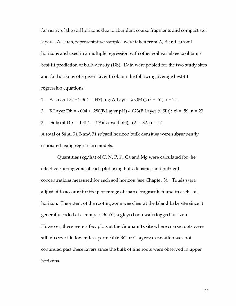
77 77
for many of the soil horizons due to abundant coarse fragments and compact soil
layers. As such, representative samples were taken from A, B and subsoil
horizons and used in a multiple regression with other soil variables to obtain a
best-fit prediction of bulk-density (Db). Data were pooled for the two study sites
and for horizons of a given layer to obtain the following average best-fit
regression equations:
1. A Layer Db = 2.864 - .449(Log(A Layer % OM)); r2 = .61, n = 24
2. B Layer Db = -.004 + .280(B Layer pH) - .023(B Layer % Silt); r2 = .59, n = 23
3. Subsoil Db = -1.454 = .595(subsoil pH); r2 = .82, n = 12
A total of 54 A, 71 B and 71 subsoil horizon bulk densities were subsequently
estimated using regression models.
Quantities (kg/ha) of C, N, P, K, Ca and Mg were calculated for the
effective rooting zone at each plot using bulk densities and nutrient
concentrations measured for each soil horizon (see Chapter 5). Totals were
adjusted to account for the percentage of coarse fragments found in each soil
horizon. The extent of the rooting zone was clear at the Island Lake site since it
generally ended at a compact BC/C, a gleyed or a waterlogged horizon.
However, there were a few plots at the Gounamitz site where coarse roots were
still observed in lower, less permeable BC or C layers; excavation was not
continued past these layers since the bulk of fine roots were observed in upper
horizons.

78 78
Average nutrient totals were described and discussed by study site and
by soil layer. Subsequently, rooting zone nutrient quantities were analysed for
spatial relationships with flow accumulation and wetness index, slope and layer-
specific texture fractions and pH through multiple and non-linear regression
analysis. Certain nutrients were log-transformed prior to analysis to approximate
normality.
RESULTS AND DISCUSSION
Overall Distribution and Trends
Bulk density increased vertically in profiles at both sites (Figure 6.1). In
comparing the two sites, the forest floor, B and subsoil layers displayed higher
bulk densities at the Island Lake site due to increased compaction in these
horizons while the Gounamitz displayed a higher mean A layer bulk density,
reflecting the predominance of finer, silty-loam textures in this horizon.
The Island Lake site showed higher average coarse fragment-weighted
totals of all nutrients and higher variation in these amounts as compared to the
Gounamitz Lake site (Table 6.1). Further, with exception of slightly higher values
for A horizon-N, K, and Ca and B horizon-P at the Gounamitz site, totals were
also higher at Island Lake for each soil layer (Table 6.1). The occurrence of fine-
grained igneous minerals in the parent material at the Island Lake site, as
opposed to the coarser sand and silt-stones at Gounamitz, likely contributed to
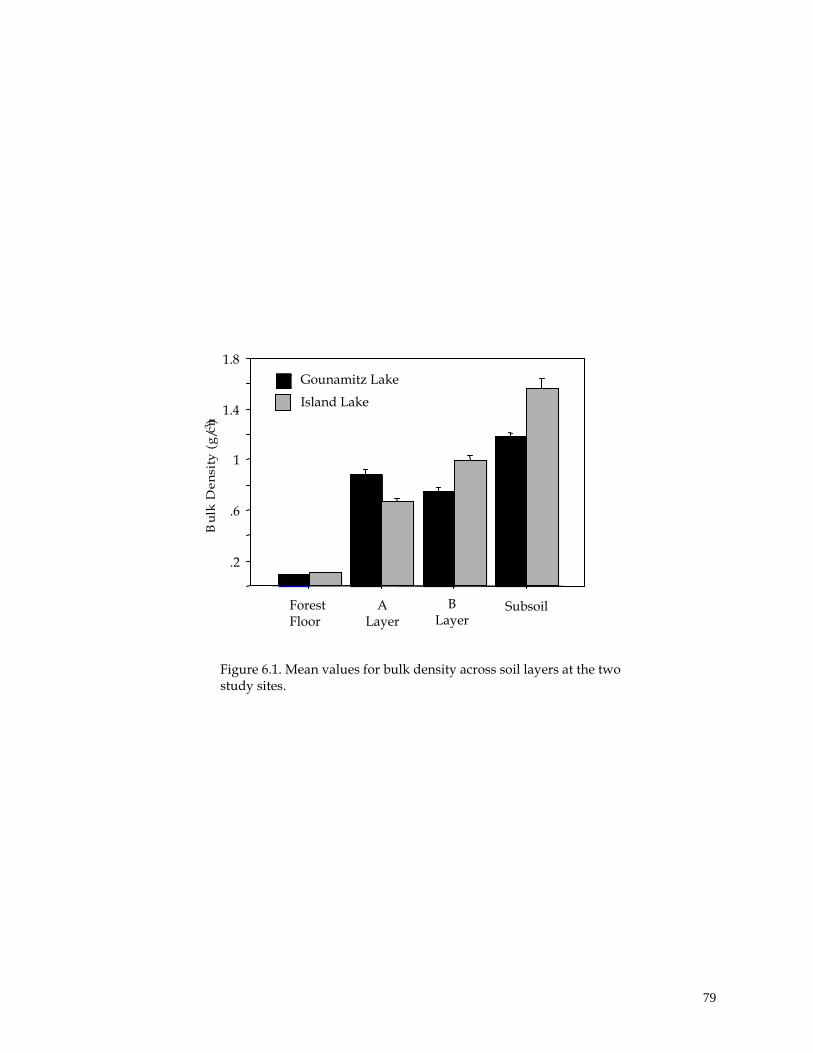
79 79
.2
.6
1
1.4
1.8
Island Lake
Gounamitz Lake
Forest Floor
A Layer
B Layer
Subsoil
Figure 6.1. Mean values for bulk density across soil layers at the two study sites.
Bu
lk D
en
sity
(g
/cm3)
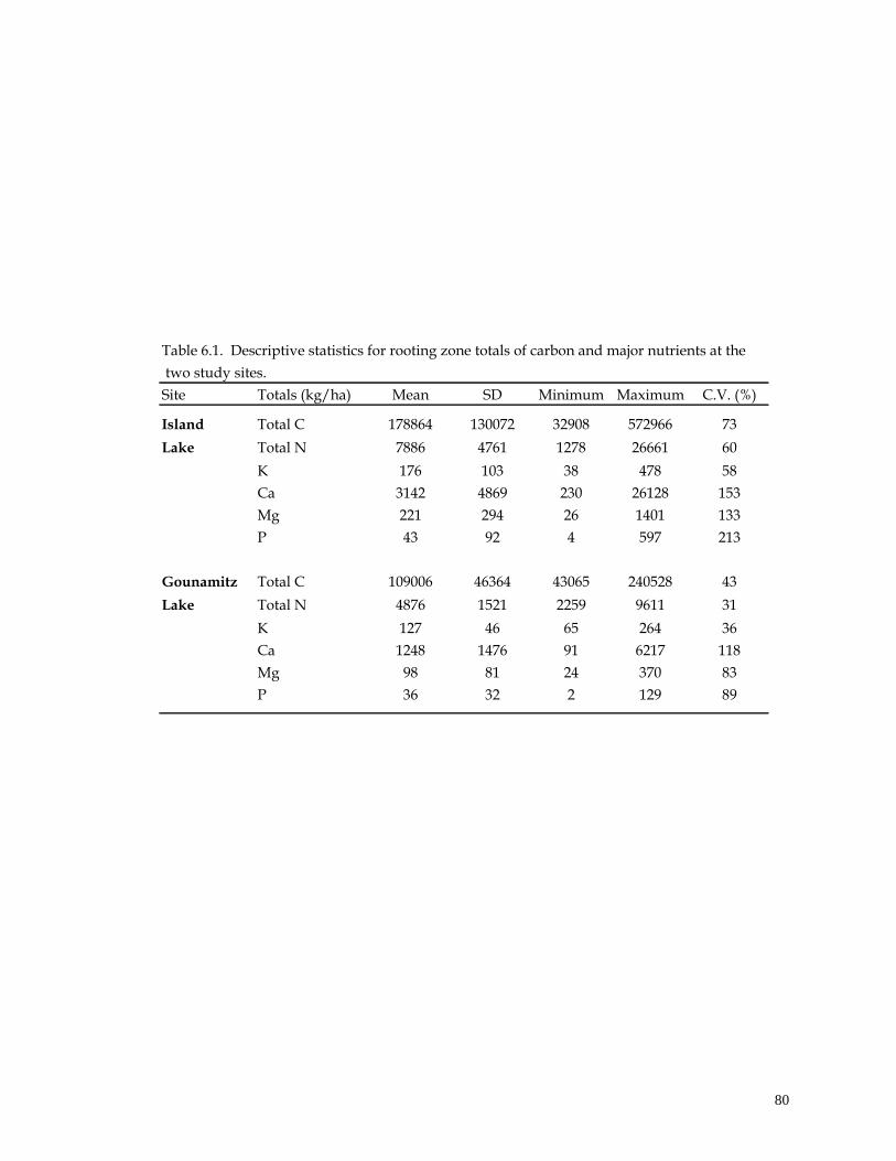
80 80
Table 6.1. Descriptive statistics for rooting zone totals of carbon and major nutrients at the
two study sites.
Site Totals (kg/ha) Mean SD Minimum Maximum C.V. (%)
Island Total C 178864 130072 32908 572966 73
Lake Total N 7886 4761 1278 26661 60
K 176 103 38 478 58
Ca 3142 4869 230 26128 153
Mg 221 294 26 1401 133
P 43 92 4 597 213
Gounamitz Total C 109006 46364 43065 240528 43
Lake Total N 4876 1521 2259 9611 31
K 127 46 65 264 36
Ca 1248 1476 91 6217 118
Mg 98 81 24 370 83
P 36 32 2 129 89

81 81
higher levels of carbon and nutrients here since less acidic parent materials
generally result in higher clay and organic matter contents (Van Cleve and
Powers 1995). Topography also exerted an influence on differences in nutrient
pools between and within sites and will be discussed later in this chapter.
Total Carbon and Nitrogen
Overall, carbon and nitrogen contents (Table 6.1) at Island Lake (Total C
= 178 Mg/ha; Total N = 7 Mg/ha) and Gounamitz Lake (Total C = 109 Mg/ha;
Total N = 4.9 Mg/ha) were comparable to values found for other studies in boreal
ecosystems. For example, Van Cleve and Powers (1995) cited a range of 149 and
170 Mg/ha for boreal ecosystem mineral soil carbon while Tetema and Verstraten
(1991) found the total N storage of the F, H and top 26 cm of mineral soil of a
Netherlands forest site to be 6.4 Mg/ha. Huang and Schoenau (1996) reported
mean total pools of 200 Mg/ha for total carbon and 8.0 Mg/ha for total nitrogen
within the forest floor and mineral soil (1m depth) at a boreal aspen forest site in
Saskatchewan. Disparities in values are partly due to the horizons and total
depths used in calculations.
Overall pooled values for total C and N were strongly correlated at both
the Island Lake (r = 0.72) and at Gounamitz (r = 0.64), as is commonly the case
(Brady 1990) and displayed similar trends across soil layers at both sites (Figure
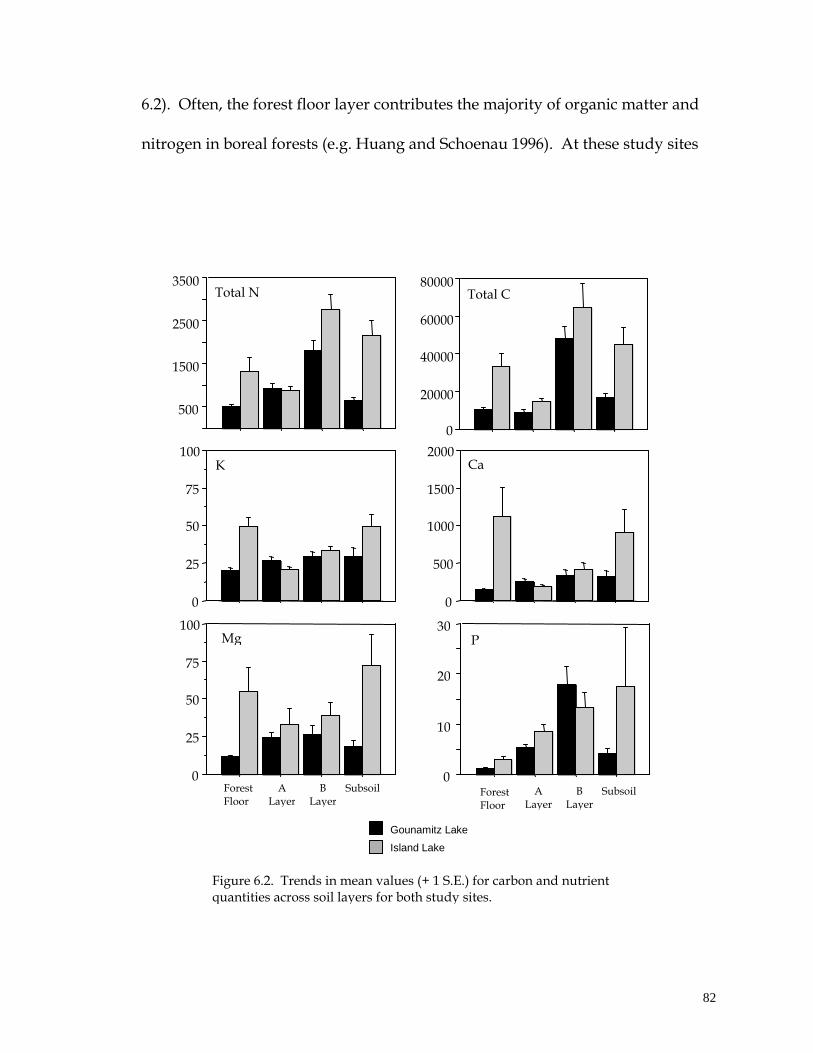
82 82
6.2). Often, the forest floor layer contributes the majority of organic matter and
nitrogen in boreal forests (e.g. Huang and Schoenau 1996). At these study sites
0
Total C (kg/ha)
20000
40000
60000
80000
0
500
1000
1500
2000 Ca (kg/ha)
0
25
50
75
100
Forest Floor
A Layer
B Layer
Subsoil
Island Lake Gounamitz Lake
Total N (kg/ha)
500
1500
2500
3500
0
25
50
75
100 K (kg/ha)
0
10
20
30 P (kg/ha)
Mg (kg/ha)
Forest Floor
A Layer
B Layer
Subsoil
Figure 6.2. Trends in mean values (+ 1 S.E.) for carbon and nutrient quantities across soil layers for both study sites.
83 83
highest totals were found within B horizons overall, as is common for soils with
podzolic profiles (David et al. 1995). There was considerable evidence of
illuviation of humic substances into the B layer, especially at the Gounamitz site;
lateral water flow and transport within this layer throughout the Island Lake site
contributed to poor soil aeration at several plots and higher storage of carbon in
mineral soil layers. Certainly, these conditions led to a much larger range of
values at Island Lake for all elements and probably resulted in relatively greater
mean values at this site.
Phosphorous
The mean amount of available phosphorous in the rooting zone totalled
43 and 36 kg/ha at the Island Lake and Gounamitz Lake site respectively (Table
6.1). Data on phosphorous quantities and forms in forest soils is less common
than other nutrients (David et al. 1995). However, the quantities calculated at
these sites agreed with the mean value of 34 kg/ha found by Huang and
Schoenau (1996) for eluviated Luvisolic soils in Saskatchewan, also analysed
using the bicarbonate method.
By soil layer, phosphorous pools were greatest in the B layer at the
Gounamitz site while both the B and subsoil layers contained the largest
proportions of P at Island Lake (Figure 6.2). The availability of phosphorous is
84 84
dependent on the weathering of primary minerals and is related to the presence
of clay, iron, aluminum and organic matter in acidic soils (Brady 1990). As has
been addressed in previous chapters, the lower mineral soil horizons in these
study sites contain a less-weathered source of coarser mineral fractions and the
lower layers were more enriched with iron, aluminum and organic matter. The
organic horizons contained the highest concentrations of available P but, on a
mass basis, comprised a relatively small pool of this nutrient.
Potassium, Calcium and Magnesium
Quantities of major cations were available in the order of Ca >> Mg >K at
Island Lake and Ca >> K > Mg at the Gounamitz site (Table 6.1). Calcium and
magnesium were especially variable at both sites, probably due to their tendency
to be highly exchangeable and mobile within the soil solution as influenced by
local pH, water flow, soil texture and organic matter.
Layer-specific stores of calcium, magnesium and potassium showed
similar within-site but different between-site trends (Figure 6.2). At Island Lake,
these nutrients generally displayed large pools in the forest floor which decreased
substantially within the A and B and increased again to relatively high quantities
in the subsoil. Organic horizons were relatively thick at this site due to
differences in spatial moisture conditions and, as a result, led to the effective
adsorption of relatively high concentrations of exchangeable cations. Conversely,
in the subsoil layers nutrient concentrations were low and comparable to A and B
85 85
layers but bulk densities were high. Plots this site receiving up-slope seepage
throughflow and groundwater inputs (Chapter 5) displayed relatively higher
cation concentrations and an increase in weathering of primary minerals, which,
at this site were partially comprised of base-rich basalt.
At Gounamitz, cation quantities increased vertically from the forest floor
to the B layer and then decreased slightly into the subsoil. Although forest floor
nutrient pools were somewhat less than mineral soil pools, the relatively thin
organic layers contributed a substantial quantity of these nutrients at this site.
Generally, results were characteristic of the well-drained podzolic soils found
here, where the B horizons provided a sink for cations as well as carbon, nitrogen
and phosphorous.
The Influence of Water Flow and Accumulation
Topography exerted both a direct and indirect influence on quantities of
C, N, P, Ca, Mg and K at both study sites. Directly, flow accumulation and
wetness index, in addition to slope gradient, were significantly related to several
nutrients at Island Lake and only to potassium at the Gounamitz site. However,
rooting zone pools were also strongly correlated with pH and clay texture
fractions for various nutrients at both sites. Both soil reaction processes and
texture influence the cycling and availability of nutrients and carbon (Kimmins
1987; Brady 1990). In this case, pH and % clay also acted as indirect and
intermediate indices of the effect of subsurface water flow and slope processes
86 86
because their distributions have been shown to be related to topography
(Chapters 4 and 5 respectively).
Total Carbon and Nitrogen
Chapter 6 illustrated the difficulty of predicting % C and % N
distributions based on topographic attributes of water flow alone. Instead, I
concluded that their distributions were likely multivariate. Results for rooting
zone storage of these nutrients were similar in this respect. Spatial distributions
of Total C pools were best explained by negative exponential relationships with
subsoil clay at Island Lake and A layer pH at Gounamitz. Total N values, on the
other hand, were linearly and positively related to flow accumulation and Total C
at the Island Lake site and to subsoil clay and Total C at Gounamitz Lake. This
latter result is not surprising given the strong co-relationship of nitrogen and
carbon.
Total C was related to both SS clay and B clay at Island Lake, although
the former provided the clearest relationship (Figures 6.3a and b). Further, the
distribution of clay increased in convergent and mildly-sloping zones as a result
of the action of subsurface water flow along impermeable subsoil layers and
accumulation in convergent zones (Chapter 4). These results, therefore, suggest
an indirect relationship between organic matter distribution and topography.
The negative functional relationship of Total C pools with clay would seem to
indirectly indicate that organic matter was greater in drier zones. Although forest
floor organic layers were thicker in wetter areas, these layers only represented a
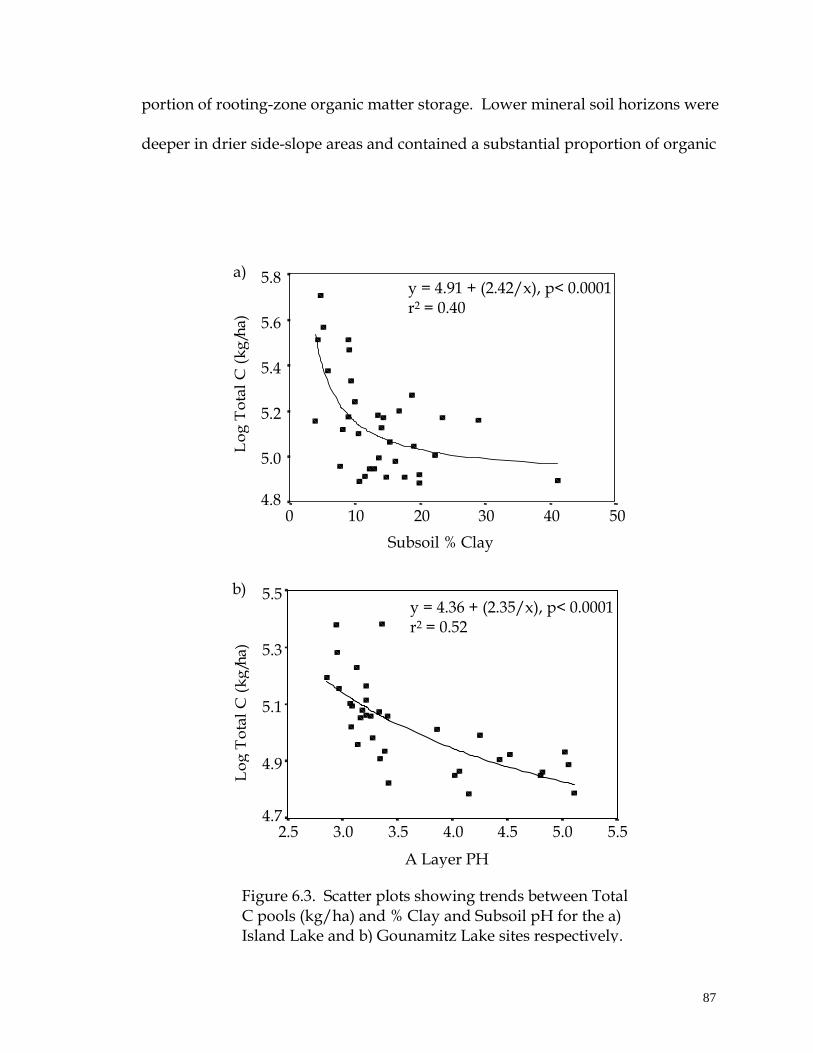
87 87
portion of rooting-zone organic matter storage. Lower mineral soil horizons were
deeper in drier side-slope areas and contained a substantial proportion of organic
b) y = 4.36 + (2.35/x), p< 0.0001 r2 = 0.52
A Layer PH
5.5 5.0 4.5 4.0 3.5 3.0 2.5
5.5
5.3
5.1
4.9
4.7
Subsoil % Clay
50 40 30 20 10 0
5.8
5.6
5.4
5.2
5.0
4.8
y = 4.91 + (2.42/x), p< 0.0001 r2 = 0.40
a)
Figure 6.3. Scatter plots showing trends between Total C pools (kg/ha) and % Clay and Subsoil pH for the a) Island Lake and b) Gounamitz Lake sites respectively.
Lo
g T
ota
l C
(k
g/h
a)
Lo
g T
ota
l C
(k
g/h
a)
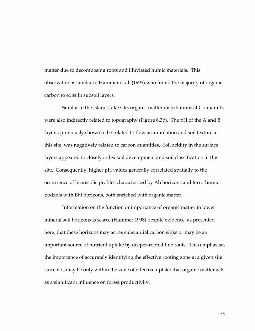
88 88
matter due to decomposing roots and illuviated humic materials. This
observation is similar to Hammer et al. (1995) who found the majority of organic
carbon to exist in subsoil layers.
Similar to the Island Lake site, organic matter distributions at Gounamitz
were also indirectly related to topography (Figure 6.3b). The pH of the A and B
layers, previously shown to be related to flow accumulation and soil texture at
this site, was negatively related to carbon quantities. Soil acidity in the surface
layers appeared to closely index soil development and soil classification at this
site. Consequently, higher pH values generally correlated spatially to the
occurrence of brunisolic profiles characterised by Ah horizons and ferro-humic
podzols with Bhf horizons, both enriched with organic matter.
Information on the function or importance of organic matter in lower
mineral soil horizons is scarce (Hammer 1998) despite evidence, as presented
here, that these horizons may act as substantial carbon sinks or may be an
important source of nutrient uptake by deeper-rooted fine roots. This emphasises
the importance of accurately identifying the effective rooting zone at a given site
since it is may be only within the zone of effective uptake that organic matter acts
as a significant influence on forest productivity.
89 89
Total nitrogen quantities co-varied strongly with carbon at both sites and
less strongly with flow accumulation and subsoil clay at Island Lake and
Gounamitz respectively (Figures 6.4a and b). This indicated that the spatial
distribution of nitrogen, while clearly dependent on carbon, is also multivariate,
4.0 3.9 3.8 3.7 3.6 3.5
3.4 3.3 3.2
4.0
3.8
3.6
3.4
3.2
Fitted
b)
Fitted
4.6 4.4 4.2
4.0 3.8 3.6 3.4 3.2 3.0
4.6
4.2
3.8
3.4
3.0
a) Y = -.39 + .164(Log Flow) + .707(Log C) p<0.0001 r2 = 0.85
Y = .94 + .014(SS %Clay) + ..514(Log C) p<0.0001 r2 = 0.53
Figure 6.4. Best-fit relationships between Total N pools (kg/ha) and topographic and soil variables for the a) Island Lake and b) Gounamitz Lake sites.
Log Total N (kg/ha)
Measured
Log Total N (kg/ha)
Measured
Log Total N (kg/ha)
90 90
responding to topographic and site influences. This supports Morris and
Boerner’s (1998) results where spatial differences in N mineralisation and nitrate
production were best explained by a host of influences including organic carbon,
pH and an integrated moisture index calculated at a meso-scale.
Phosphorous
Phosphorous quantities for the rooting zone correlated negatively and
non-linearly with flow accumulation at the Island Lake site (Figure 6.5a). This
trend suggested that toe-slopes and other areas of convergence, where water
accumulation was greatest, were areas of least P availability at this site. Instead,
P quantities were highest along mid and lower slope areas where P accumulated
due to down-slope through-flow of subsurface water, as in Xiao et al.’s (1991)
study. Areas with increased water through-flow would also have a concomitant
increase in mineral weathering, the predominate source of this element.
Conversely, across the Gounamitz Lake site, P quantities were positively
related to carbon and negatively related to surface pH distributions (Figure 6.5b).
This finding makes sense since phosphorous availability is known to be adsorbed
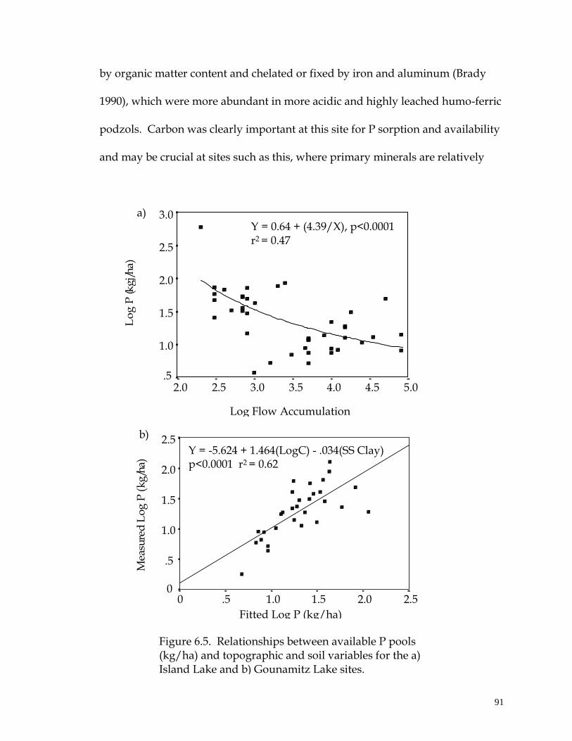
91 91
by organic matter content and chelated or fixed by iron and aluminum (Brady
1990), which were more abundant in more acidic and highly leached humo-ferric
podzols. Carbon was clearly important at this site for P sorption and availability
and may be crucial at sites such as this, where primary minerals are relatively
Fitted Log P (kg/ha)
2.5 2.0 1.5 1.0 .5 0
2.5
2.0
1.5
1.0
.5
0
Y = -5.624 + 1.464(LogC) - .034(SS Clay) p<0.0001 r2 = 0.62
Log Flow Accumulation
5.0 4.5 4.0 3.5 3.0 2.5 2.0
3.0
2.5
2.0
1.5
1.0
.5
Y = 0.64 + (4.39/X), p<0.0001 r2 = 0.47
Figure 6.5. Relationships between available P pools (kg/ha) and topographic and soil variables for the a) Island Lake and b) Gounamitz Lake sites.
b)
a)
Lo
g P
(kg
j/h
a)M
easu
red
Lo
g P
(k
g/h
a)
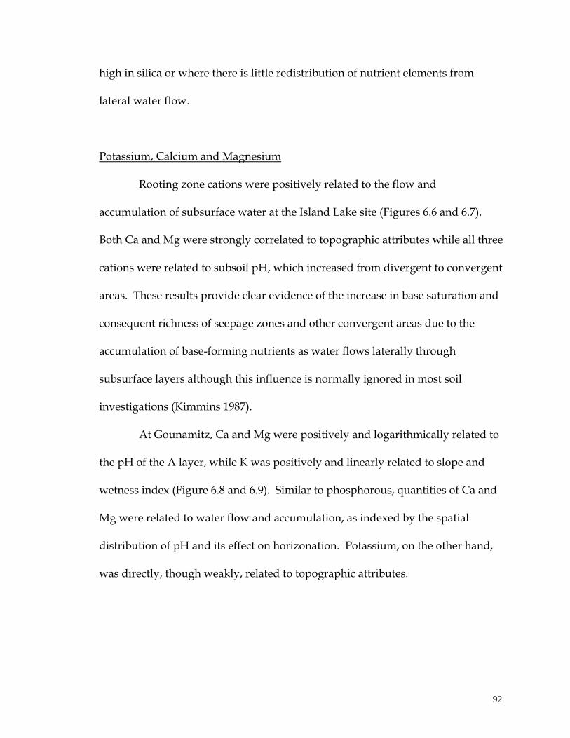
92 92
high in silica or where there is little redistribution of nutrient elements from
lateral water flow.
Potassium, Calcium and Magnesium
Rooting zone cations were positively related to the flow and
accumulation of subsurface water at the Island Lake site (Figures 6.6 and 6.7).
Both Ca and Mg were strongly correlated to topographic attributes while all three
cations were related to subsoil pH, which increased from divergent to convergent
areas. These results provide clear evidence of the increase in base saturation and
consequent richness of seepage zones and other convergent areas due to the
accumulation of base-forming nutrients as water flows laterally through
subsurface layers although this influence is normally ignored in most soil
investigations (Kimmins 1987).
At Gounamitz, Ca and Mg were positively and logarithmically related to
the pH of the A layer, while K was positively and linearly related to slope and
wetness index (Figure 6.8 and 6.9). Similar to phosphorous, quantities of Ca and
Mg were related to water flow and accumulation, as indexed by the spatial
distribution of pH and its effect on horizonation. Potassium, on the other hand,
was directly, though weakly, related to topographic attributes.
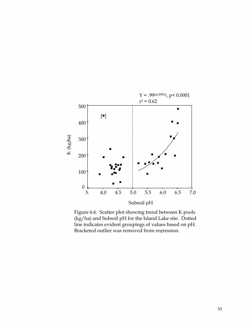
93 93
Subsoil pH
7.0 6.5 6.0 5.5 5.0 4.5 4.0 3.5
500
400
300
200
100
0
Figure 6.6. Scatter plot showing trend between K pools (kg/ha) and Subsoil pH for the Island Lake site. Dotted line indicates evident groupings of values based on pH. Bracketed outlier was removed from regression.
Y = .99(e(.89X)), p< 0.0001 r2 = 0.62
[ ]
K (
kg
/ha)
94 94
Fitted Log Ca (kg/ha)
5.0 4.5 4.0 3.5 3.0 2.5 2.0
5.0
4.5
4.0
3.5
3.0
2.5
2.0
Fitted Log Mg (kg/ha)
3.5 3.0 2.5 2.0
1.5 1.0
3.5
3.0
2.5
2.0
1.5
1.0
Y = .468 + .172(LogFlow) + .419(SS pH) p<0.0001 r2 = 0.79
Y = .114 + .035(WI) + .354(SS pH) p<0.08 r2 = 0.68
Figure 6.7. Best-fit relationships between available a) Ca and b) Mg pools (kg/ha) and topographic and soil variables for the Island Lake site.
Measu
red
Lo
g C
a (
kg
/ha)
Measu
red
Lo
g C
a (
kg
/ha)
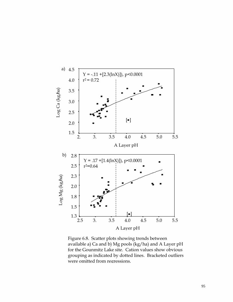
95 95
A Layer pH
5.5 5.0 4.5 4.0 3.5 3.0
2.5
4.5
4.0
3.5
3.0
2.5
2.0
1.5
A Layer pH
5.5 5.0 4.5 4.0 3.5 3.0
2.5
2.8
2.5
2.3
2.0
1.8
1.5
1.3
Figure 6.8. Scatter plots showing trends between available a) Ca and b) Mg pools (kg/ha) and A Layer pH for the Gounmitz Lake site. Cation values show obvious grouping as indicated by dotted lines. Bracketed outliers were omitted from regressions.
Y = -.11 +[2.3(lnX)]), p<0.0001 r2 = 0.72
Y = .17 +[1.4(lnX)]), p<0.0001 r2=0.64
a)
b)
[ ]
[ ]
Lo
g C
a (
kg
/ha)
Lo
g M
g (
kg
/ha)
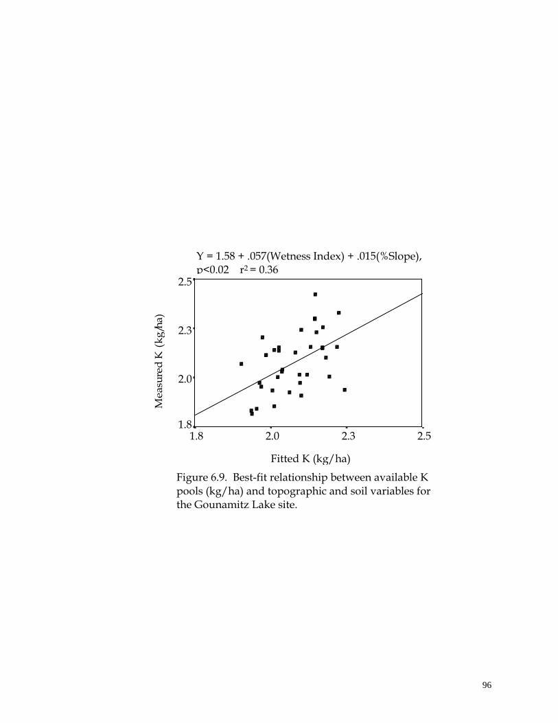
96 96
Fitted K (kg/ha)
2.5 2.3 2.0 1.8
2.5
2.3
2.0
1.8
Figure 6.9. Best-fit relationship between available K pools (kg/ha) and topographic and soil variables for the Gounamitz Lake site.
Y = 1.58 + .057(Wetness Index) + .015(%Slope), p<0.02 r2 = 0.36
Measu
red
K (
kg
/ha)
97 97
SUMMARY
Rooting zone quantities of carbon, nitrogen, phosphorous and nutrient cations
varied substantially across two headwater catchment study areas. Spatial
analyses suggested that relatively simple yet significant functional relationships
existed between spatial patterns of available nutrients, indices of water flow and
accumulation, soil acidity and soil texture, although these trends differed by site.
Results also suggested that carbon and nitrogen, phosphorous, and the three
cations (K, Ca, Mg) formed three separate functional groups that responded to
similar landscape factors within a site.
The range of spatially aggregated rooting zone values for carbon,
nitrogen and phosphorous were found to be similar to other investigations
carried out in a boreal forest setting although these studies differed in terms of
the soil depth used to characterise the vertical extent of available soil nutrients.
Kimmins (1987, p. 246) noted this as a potential problem in nutrient studies since
the depth of maximum rooting does not necessarily equate to the sorption zone of
a given root system. In this analysis, only horizons with fine roots were included
as a part of the effective rooting zone.
Spatially, available nutrients were either indirectly or directly related to
lateral and vertical water flow and accumulation processes occurring at both
sites, although trends were specific to each site. At the Island Lake site, where
98 98
there was strong lateral water flow and accumulation due to impermeable subsoil
zones, expected flow accumulation and wetness index values were significant
indicators of N, P, Ca and Mg pools. Additionally, subsoil pH and/or % Clay
were also strongly related to all nutrients; these factors, previously shown to be
highly related to topographic indices, are functional indicators of seepage
influences along lower mineral horizon layers at this site.
Topographic indices were much less influential at the Gounamitz site
while processes influencing the pH of surface layers across this site were more
important indicators of rooting zone nutrient quantities. Soil descriptions
identified strong spatial differences in A horizon development at this site and
previous results showed that A horizon pH distributions were at least partially
the result of lateral water movement, although to a lesser degree than at Island
Lake.
Delineating adequate indicators of nutrient and carbon pools at these
sites are clearly complex and data regarding micro-climatic (e.g. soil temperature)
and temporal nutrient turnover influences may shed further light on this matter.
Spatial patterns of soil nutrients as presented here would certainly be more
ecologically meaningful in the context of tree uptake and growth (Silver et al.
1994). This work would benefit greatly from a more complete analysis of
biogeochemical differences between and within the conifer stands dominating
Island Lake site and tolerant hardwood forest found at the Gounamitz Lake site.
This would provide a clearer picture of how the sites and plots differ with respect

99 99
to nutrient demand, nutrient partitioning, rooting distribution, turnover rates
and, ultimately, whether the influence of water flow and accumulation is
expressed above-ground as within the soil medium.
100 100
CHAPTER 7
TWO SURVEY METHODS FOR CREATING FINE-SCALE DEM’S UNDER
A FOREST CANOPY: A QUALITATIVE ANALYSIS
INTRODUCTION
In light of the concerns presented earlier in this thesis, there is a clear
need for exploring methods of obtaining accurate elevation data at a meso-scale
such that local topographic complexity is adequately represented. This fine-scale
characterisation is crucial in ecological studies where the aim is to identify and
understand local topographic influences on meso to micro-scale ecological
processes.
Meso-scale investigations relating DEM-derived attributes to soil
properties within agricultural field sites, carried out by Odeh et al. (1991) and
Moore et al. (1993), used fine-scale data generated from field surveys using
traditional survey equipment. Similarly, Wilson et al. (1998) used a high
precision truck-mounted Global Positioning System (GPS) on a farm field to
derive fine-scale elevation data while Dietrich et al. (1993) used digital
photgrammetry for a sparsely vegetated site. Unfortunately, these methods are
useless in areas of dense forest cover as found at the Island Lake site.
101 101
As such, presented in this chapter are two field techniques for generating
relatively fine-scale elevation data under thick to moderate forest canopy
conditions using both manual methods and a hybrid manual/GPS procedure.
Elevation data collected using these methods are used to create two DEM’s for a
sub-section of the Island Lake site and are compared to Provincial DEM’s to
illustrate the effect of scale.
METHODS
Two Field Survey Methods For Creating a Fine-Scale DEM
Polychain Method
A section of the Island Lake site (~7.5 ha) covering most of the lower part
of sub-catchment 1 was used as the study area for demonstrating this survey
approach. This areas was selected because it consisted of a well-defined gully
(representative of hummocky terrain) with a central intermittent flow channel
that could not be resolved using the provincial elevation data set.
Traditional survey methods using either a normal transit or a laser transit
were initially considered but rejected for two main reasons. First of all, these
methods require that the transit be levelled for each new survey section and that
the target be visible to acquire measurements. The Island Lake site, however,
contained many dense stands of black spruce and balsam fir, which rendered
these methods too time-consuming to use. Secondly, the aim was to achieve
better overall representation and relative accuracy of elevations, and the higher
precision of traditional survey methods was deemed unnecessary.
102 102
Several control points of known elevations were identified along a ridge
area and along a nearby logging trail and were used to geo-reference the
surveyed points. Transects, spaced at 25 m, were established at a given compass
direction perpendicular to the gully slopes such that maximum differences in
slope change were measured.
The survey was carried out with two people: a chain-bearer and a note-
taker. The chain-bearer, carrying the 0 m end of a 50 m polychain, followed a
pre-set bearing until a perceived break in slope was encountered, or until
visibility was lost due to forest conditions, and subsequently established a station
at that location. At this point, to minimise errors due to inaccurate navigation
along the bearing, the path taken by the chain-bearer was verified by the note-
taker using his/her compass, and lateral adjustments were made accordingly. At
each station a distance and % slope reading, between the note-taker to the chain-
bearer, was measured using the polychain and Suunto clinometer respectively.
GPS Method
As a possibly less time-consuming alternative to the above field survey
method, a trial approach using Corvallis Microtechnology MC-GPS, C/A code
receivers (horizontal accuracy of 3-5 m after correction) was carried out to cover
an area comprising the remaining unsurveyed portion of sub-catchments 1 and 2
at Island Lake. Using a nearby road and several ridge high points as control
points, transects at ~50m intervals were established and traversed by a crew of
103 103
three people. Two people, each with a GPS receiver, followed a general bearing
from the note-taker, perpendicular to the prevalent slope gradient. To cover
more area efficiently, two procedures were used depending on the complexity of
terrain:
1. In less complex terrain (i.e. less hummocky) the first GPS user followed a
bearing set by the note-taker and proceeded to the next break in slope while
the second GPS user continued past the first, along the same bearing, until the
next successive slope-break was encountered. A % slope reading was taken
by the note-taker to the first GPS user while both GPS users recorded GPS
positions at their given stations. During this time, the note-taker proceeded to
the location of the nearest GPS-user and took another slope reading to the
second GPS user. The first GPS user then set out again along the same bearing
locating the next slope break. Thus point locations and slope measurements
were taken in a “leap-frog” manner along a particular compass direction.
2. Alternately, in more locally complex terrain, one GPS user was used as a
“floater” and directed by the note-taker to acquire GPS positions at nearby
landform features (hummocks or depressions) not on the transect route that
were deemed substantial enough to affect the proper characterisation of
meso-scale topography. The other GPS user continued, as in the first method,
to the next break in slope along the original transect bearing. Slope readings
to each GPS user and GPS positions were taken as described earlier and then
each GPS user and the note-taker proceeded along the transect to another set

104 104
of points in this fashion. This more flexible method attempted to identify
and account for obvious features in this terrain that may have been missed by
stringently following a transect route.
Six ten-second GPS points were recorded at each station and each
recorded point was comprised of ten positions (one per second). For most cases,
positions were only recorded when the receiver was tracking enough satellites to
acquire a 3D fix. This meant that 4 or more satellites were being adequately
tracked; at times, due to poor satellite geometry, thick forest canopy or inclement
weather, positions were recorded from only 3 satellites.
Positions, identified by station number, were downloaded from the GPS
receiver to a laptop computer and differentially corrected with data collected for
that given day at a base-station 50 km away in Dalhousie, NB. Each set of
corrected positions at a given elevation point were viewed with MC-GPS
software, obvious outlier points were discarded, and the remaining cluster of
points were averaged to give a mean location for each point. The six point values
were then averaged to provide mean location for a station. These multiple
measurements, in effect, helped isolate and minimise positional dilution of
precision (PDOP) error due to the temporary loss or poor positioning of satellites
or inadequate reception. By geo-referencing at least one end of each transect
relative to known control points, elevations were calculated using the slope
measurements taken from point to point.

105 105
Organisation and Analysis of Survey Data
Using known control points, obtained from a 1: 10 000 ortho-photo
topographic map, elevations could be calculated along transects for both
methods. For the Polychain method, simple geometrical relationships were
applied to derive X and Y co-ordinates for each point and the vertical rise for each
interval using distance and % slope measurements along a known bearing. Each
successive transect was connected to the previous transect, allowing a grid of
elevations to be developed. The GPS method simplified these calculations since
the X and Y co-ordinates were automatically positioned and only the vertical rise
needed to be calculated using percent gradient measurements from point to
point.
Figures 7.1a and b display the distribution of elevation points as derived
using the two survey methods as well as those obtained from the Province of
New Brunswick respectively. Points surveyed using the Polychain procedure are
presented in Figure 7.1a as an outlined grid of points imbedded within the
elevation grid created using the GPS method. DEM’s were created by
interpolating these irregular elevation grids (Vertical Mapper Software v.2 1998)
to regular 10 and 15 m grids for the Polychain and GPS data-sets respectively;
New Brunswick Provincial elevation data were also interpolated to the same
resolution for corresponding areas. These two sets of DEM’s were examined
qualitatively to assess the ability of the two methods to characterise topography
in comparison to two provincial DEM’s covering the same spatial extent.
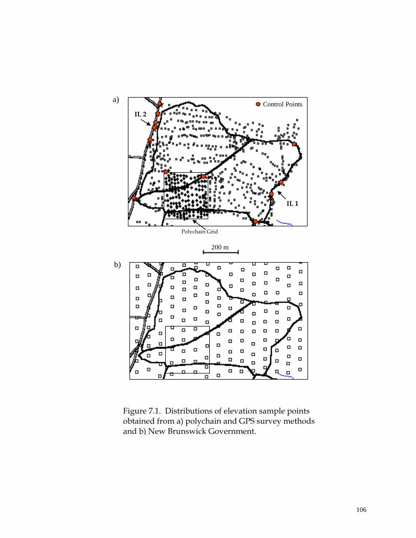
106 106
Control Points
IL 1
IL 2
Polychain Grid
200 m
Figure 7.1. Distributions of elevation sample points obtained from a) polychain and GPS survey methods and b) New Brunswick Government.
b)
a)
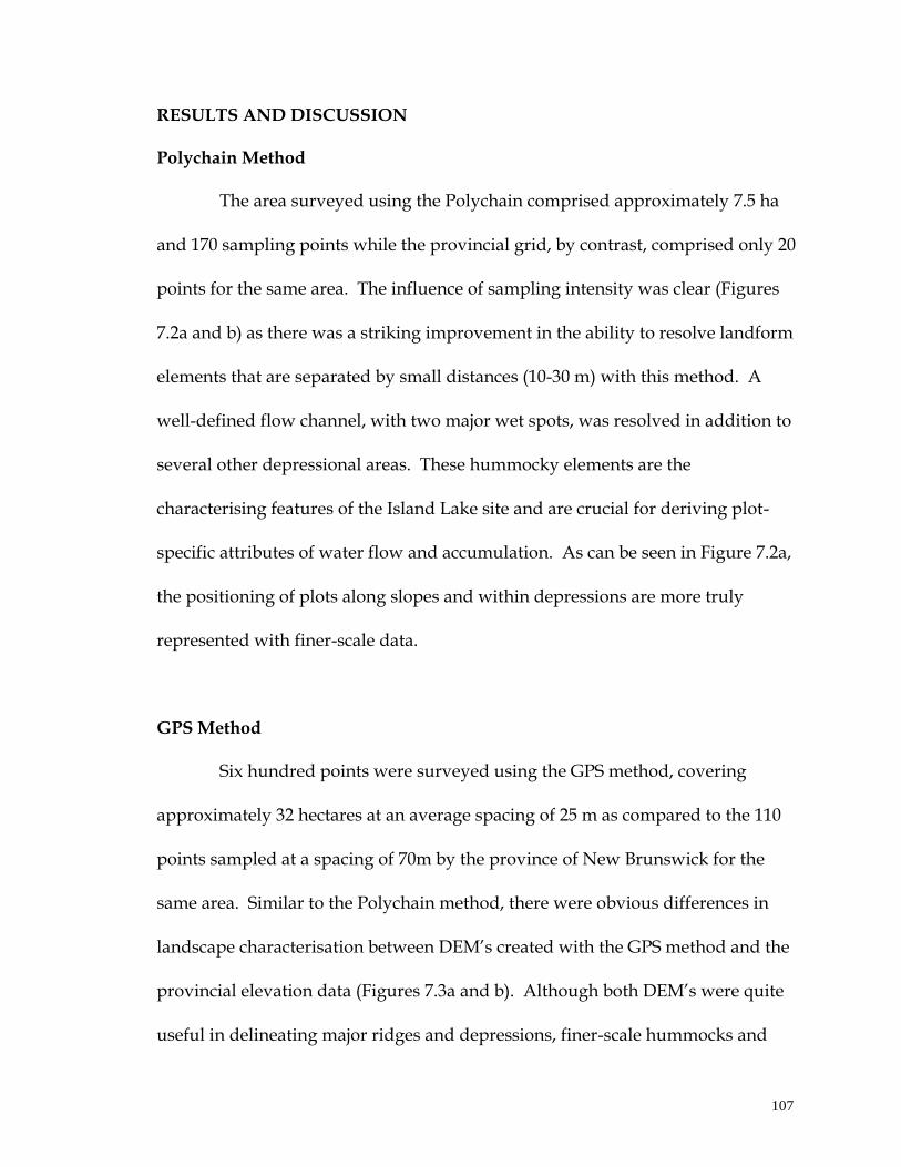
107 107
RESULTS AND DISCUSSION
Polychain Method
The area surveyed using the Polychain comprised approximately 7.5 ha
and 170 sampling points while the provincial grid, by contrast, comprised only 20
points for the same area. The influence of sampling intensity was clear (Figures
7.2a and b) as there was a striking improvement in the ability to resolve landform
elements that are separated by small distances (10-30 m) with this method. A
well-defined flow channel, with two major wet spots, was resolved in addition to
several other depressional areas. These hummocky elements are the
characterising features of the Island Lake site and are crucial for deriving plot-
specific attributes of water flow and accumulation. As can be seen in Figure 7.2a,
the positioning of plots along slopes and within depressions are more truly
represented with finer-scale data.
GPS Method
Six hundred points were surveyed using the GPS method, covering
approximately 32 hectares at an average spacing of 25 m as compared to the 110
points sampled at a spacing of 70m by the province of New Brunswick for the
same area. Similar to the Polychain method, there were obvious differences in
landscape characterisation between DEM’s created with the GPS method and the
provincial elevation data (Figures 7.3a and b). Although both DEM’s were quite
useful in delineating major ridges and depressions, finer-scale hummocks and
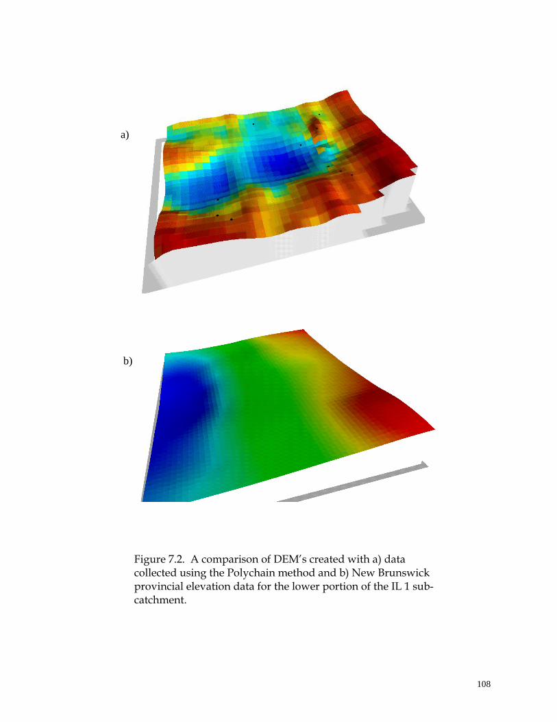
108 108
Figure 7.2. A comparison of DEM’s created with a) data collected using the Polychain method and b) New Brunswick provincial elevation data for the lower portion of the IL 1 sub-catchment.
a)
b)
109 109
Figure 4.3. A comparison of DEM’s created with a) data collected using the polychain/GPS methods and b) NB provincial elevation data for the IL 1 and 2 sub-catchments.
a)
b)
110 110
depressions were better represented with the GPS method. Additionally, the
definition of the lower sections of the two watersheds (Figure 7.3a, bottom left)
was more accurate and representative of field conditions. These lower areas are
crucial in deriving water flow networks since they are confluence points for up-
slope drainage.
Identifying Sources of Error: A Caveat
For either method described above, there are two main sources of
potential error: positional error in horizontal co-ordinates and elevation or
vertical dimension error.
Using the Polychain method, positional error arises from small deviations
between the set transect bearing and the path actually followed in the field. This
error was somewhat minimised by having the two surveyors correct each other’s
bearing from point to point until a location was agreed upon. This error could be
potentially worse along longer transects since it may accumulate over distance.
However, if spacings between transects are relatively small and the transects
themselves are short, the amount of error in calculations would be negligible.
Error in this study using the Polychain method was considered reasonable at ±2
metres.
Although the GPS method was somewhat faster than the Polychain
method, there are potentially more sources of error in positional accuracy
including: poor satellite geometry, receiver clock error, multipath error (e.g. from
111 111
tree crowns), and atmospheric interference (French 1996). In this study, satellites
were periodically lost and gained causing a range in Positional Dilution of
Precision (PDOP) error from 2 to 8, although values were generally lower than 5.
It is recommended that a position be recorded only if the PDOP value is between
2 and 6 (French 1996; Darche and Forgues 1998).
Accurate characterization of point elevations is dependent on the
accurate determination of horizontal co-ordinates as well as the proper
characterization and measurement of slope gradient cumulatively from point to
point. Inaccurate horizontal locations influence calculated distances between
points and, consequently, calculated elevation values. For example for a
measured slope gradient of 10 % between points spaced at 20 m in the field, the
vertical rise is 1.99 m. If, however, the distance between the same two points
using either survey method was inappropriately measured as 15 m, the vertical
rise now becomes 2.23 m, an increase in elevation of 0.24 m. Although this is a
seemingly small value, this error can accumulate over space. I suspect that this
was more of a potential problem here with the GPS method because positional
error could have been up to 5 m in any direction and because transects were
fairly long (200 – 400 m).
Additionally, it is crucial that control points be accurate and abundant to
allow for proper geo-referencing of point values. In this study elevation values of
control points were estimated from ortho-photo maps and were therefore
112 112
dependent on the accuracy of map contours and the ability to accurately measure
locations from the map.
SUMMARY AND RECOMMENDATIONS
Both the Polychain and GPS methods outlined in this Chapter show
much promise in improving the characterization of fine-scale topography. In
comparing Digital Elevation Models created from surveyed elevation data and
those available from the province of New Brunswick, it was clear that the former
were better able to resolve such fine-scale landform features as local depressions,
hummocks and flow channels; these features are characteristic of the Island Lake
area and are important determinants of water flow and accumulation. The
Polychain method, though somewhat more time consuming, may be more
appropriate in areas such as this where landform changes are frequent. The GPS
method is potentially more efficient but care must be taken to obtain accurate
positions at each point with no less than four satellites. The consequences of the
±5m receiver error in this study may not be as detrimental in areas of more
subdued or rolling topography.
To minimize potential positional and vertical error, I suggest that:
1. Accurate control points be established at the beginning of each new transect if
possible. A dual frequency GPS unit would provide extremely accurate X,Y

113 113
and Z positions for control points in open areas as compared to deriving
values from contour maps.
2. Transects be laid out perpendicular to the slope gradient and kept relatively
short to minimize cumulative error. To facilitate this, accurately geo-
referenced baselines could be initially established as known start and end
points for transects.
3. The density of transects be varied depending on the complexity of topography
in a given area. This will help maximise overall accuracy and area coverage
and increase efficiency.
4. A clear record be kept of DOP values and the number of satellites used to
locate a given position so that errant points can be identified later. To
minimise error further, GPS positions should be recorded only when adequate
satellites are being tracked and when DOP values are below the five to six
range.
114
CHAPTER 8
THESIS CONCLUSION
SYNTHESIS
The relationship between lateral water flow and soil development and
distribution has long been suggested in theory by Jenny (1941, 1980), Hugget
(1975) and Conacher and Dalrymple (1977) while investigations, varying in study
design and scale, have provided substantial supporting evidence (e.g. Walker et
al. 1968; King et al. 1983; Pennock 1987; Carter and Ciolkosz 1991; Hairston and
Grigal 1991; Odeh et al. 1991; Brubaker et al. 1993; Moore et al. 1993). In this
study, flow accumulation and steady-state wetness index were examined as
predictive indices of soil property distributions mainly because: (1) they are
recognised as important, hydrologically-significant indices of lateral subsurface
water flow (Speight 1974; O’Loughlin 1986; Moore et al. 1991, 1993, 1996); (2) they
have rarely been used to predict soil chemical and physical property
distributions; and (3) such metrics provide a better means of identifying and
delineating the possible quantitative form and function of established
relationships.
Initially, it was clear that elevation data readily available from the
Province of New Brunswick were too coarse to adequately characterise
topography and to automatically derive topographic metrics at this study scale.
Systematically derived “expected values” of flow accumulation and wetness

115 115
index, although based mainly on field observations, were a justified comparison
in this case given available data. Expected values were verified to the extent that
they correlated with soil drainage at Island Lake and soil horizonation at
Gounamitz Lake. In retrospect, it would have been more valid to measure and
document the presence, depth, direction, and amount of laterally-flowing water
at points within a given flow catchment, especially at high flow periods. This
would have provided a more quantitative validation of the nature of lateral water
flow at a field level.
Admittedly, the desired aim is the ability to adequately and accurately
derive consistent values for a range of hydrologic attributes using automatic
methods for any point in the landscape (Moore et al. 1993). Results presented in
this thesis, however, indicate that elevation data must be of fine enough
resolution to characterise topographic variation at the proposed scale of study.
Few past studies in the available literature have discussed scale effects and the
adequacy of available topographic data; field-level verification of these data is
essential, especially since topography provides the foundation for many
landscape studies.
A main problem in remote areas such as the Island Lake and Gounamitz
Lake sites is the lack of an efficient way to obtain fine-scale elevation data with
automatic methods due to thick forest cover. The two field-level survey methods
presented in this thesis clearly improved the characterisation of meso-scale
topography and thus demonstrate a legitimate way to obtain elevation data,
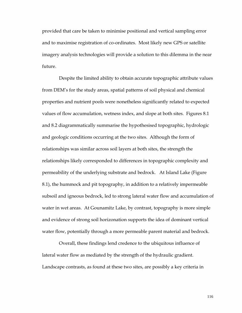
116 116
provided that care be taken to minimise positional and vertical sampling error
and to maximise registration of co-ordinates. Most likely new GPS or satellite
imagery analysis technologies will provide a solution to this dilemma in the near
future.
Despite the limited ability to obtain accurate topographic attribute values
from DEM’s for the study areas, spatial patterns of soil physical and chemical
properties and nutrient pools were nonetheless significantly related to expected
values of flow accumulation, wetness index, and slope at both sites. Figures 8.1
and 8.2 diagrammatically summarise the hypothesised topographic, hydrologic
and geologic conditions occurring at the two sites. Although the form of
relationships was similar across soil layers at both sites, the strength the
relationships likely corresponded to differences in topographic complexity and
permeability of the underlying substrate and bedrock. At Island Lake (Figure
8.1), the hummock and pit topography, in addition to a relatively impermeable
subsoil and igneous bedrock, led to strong lateral water flow and accumulation of
water in wet areas. At Gounamitz Lake, by contrast, topography is more simple
and evidence of strong soil horizonation supports the idea of dominant vertical
water flow, potentially through a more permeable parent material and bedrock.
Overall, these findings lend credence to the ubiquitous influence of
lateral water flow as mediated by the strength of the hydraulic gradient.
Landscape contrasts, as found at these two sites, are possibly a key criteria in
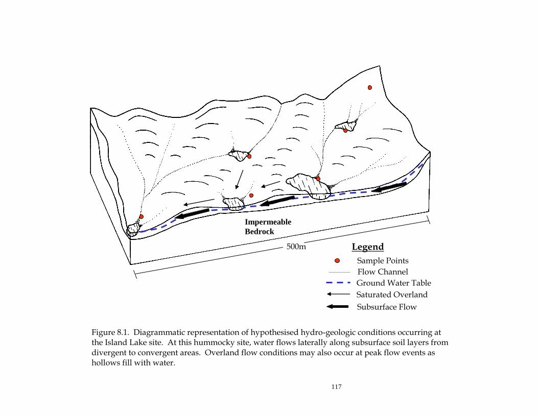
117
Figure 8.1. Diagrammatic representation of hypothesised hydro-geologic conditions occurring at the Island Lake site. At this hummocky site, water flows laterally along subsurface soil layers from divergent to convergent areas. Overland flow conditions may also occur at peak flow events as hollows fill with water.
Impermeable
Bedrock
Legend
Flow Channel
Ground Water Table
Sample Points
Saturated Overland Flow Subsurface Flow
500m
117
200m
Soil
Figure 8.2. Diagrammatic representation of hypothesised hydro-geologic conditions present at the Gounamitz Lake site. Vertical water flow through soil parent material and fractured bedrock outweighs surface and subsurface flow at this rolling site.
Legend
Flow channel Ground water table
Sample points
Fractured Rock
Impermeable Rock
119
garnering a better understanding of ecological processes that are potentially
common across landscapes.
Although the topographic attributes employed showed substantial
spatial correlation with soil properties, results also suggested that soil chemicals
and total nutrient pools were partially related to parent material. The
multivariate nature of soil development, as influenced by a host of “state factors”
(Jenny 1980), is widely recognised. Certainly there is a degree of randomness in
the distribution of physical soil variables, as outlined in Chapter 4, that is
especially evident in glacial environments. I suspect, however, that a greater
proportion of unexplained variance could be accounted for in this study by
including micro- or meso-scale climatic factors and by exploring other metrics
that accurately describe landform shape, water flow and moisture conditions.
Further, this study essentially represents one sample in time; temporal
fluctuations in chemical properties in particular may be substantial (Hammer et
al. 1987) and should not be ignored.
OVERALL CONTRIBUTIONS
In the context of soil-landscape research, this thesis has provided the
following main contributions:
1. A thorough synthesis of methodologies and outcomes of previous
investigations concerning water flow and accumulation and its influence on
soil properties in a spatial context;

120 120
2. Results that support the working hypothesis that soil physical and chemical
properties vary horizontally and vertically at relatively fine scales, largely due
to the degree of terrain divergence/convergence, slope position, and the
resultant effect of lateral surface and subsurface water flow;
3. Evidence that the function of water flow, as measured in this study, is
ubiquitous and the strength of its influence is mediated by the complexity of
the local topography and the permeability of the solum and underlying
substrate;
4. Statistical evidence of the underlying form of potential relationships between
flow accumulation, soil physical characteristics, and soil chemistry.
Indirectly, this thesis has also provided further support for using
watersheds as functional ecological units. Watersheds provide the logical
framework for investigations concerning hydrologic processes because they are
self-contained, defined by local topography, hierarchically structured, and easily
delineated with automatic methods. Watershed investigations are clearly quite
relevant from a forestry perspective since knowledge of water flow and quality is
one of the basic determinants of forest productivity. Headwater stream
watersheds are of moderate relief and, as such, are areas that are frequently
accessible for harvesting. Intermittent feeder streams within these sites,
therefore, play an important role in contributing to the overall water quality of
higher order streams, and yet are generally overlooked during harvest.

121
Investigations such as this, at the very least, create a greater awareness of
the importance of headwater streams and may contribute to the establishment of
specific best management practices (BMP’s) for forestry activities such as road
location, harvesting methods, and buffer-strip design.
122
LITERATURE CITED
Aandahl, A.R. 1948. The characterisation of slope positions and their influence
on the total nitrogen content of a few virgin soils of western Iowa. Proc.
Soil Sci. Soc. Am. 13: 449-454.
Arrouays, D., J. Daroussin, J-L. Kicin, and P. Hassika. 1998. Improving topsoil
carbon storage prediction using a digital elevation model in temperate
forest soils of France. Soil Sci. 163: 103-108.
Band, L.E., P. Patterson, R. Nemani, and S.W. Running. 1993. Forest ecosystem
processes at the watershed scale: incorporating hillslope hydrology. Agric.
For. Meteorol. 63: 93-126.
Bevin, K.J. and M.J. Kirkby. 1979. A physically-based variable contributing area
model of basin hydrology. Hydro. Sci. Bull. 24: 43-69.
Boudeman, J.W. 1989. Above- and below-ground production of three forage
legumes related to soil properties and a soil-based productivity index.
M.S. Thesis, Univ. Missouri-Columbia.
Brady, N.C. 1990. The nature and properties of soils: 10th edition. Macmillan
Publishing Co., New York, N.Y. 621 pages.
Brasington, J. and K. Richards. 1998. Interactions between model predictions,
parameters and DTM scales for TOPMODEL. Comp. Geosci. 24: 299-314.
Brubaker, S.C., A.J. Jones, D.T. Lewis, and K. Frank. 1993. Soil properties
associated with landscape position. Soil Sci. Soc. Am. J. 57: 235-239.
123 123
Burt, T.P. and D.P. Butcher. 1985. Topographic control of soil moisture
distributions. J. Soil Sci. 36: 469-486.
Burt, T.P. and D.P. Butcher. 1986. Development of topographic indices for use in
semidistributed hillslope runoff models. In: Geomorphology and Land
Management. pp. 1-19. Edited by O. Slaymaker and D. Balteanu.
Gebruder Borntraeger, Berlin.
Carter, B.J. and E.J. Ciolkosz. 1991. Slope gradient and aspect effects on soils
developed from sandstone in Pennsylvania. Geoderma. 49: 199-213.
Colpitts, M.C., S.H. Fahmy, J.E. MacDougall, T.T.M. Ng, B.G. McInnis and V.F.
Zelazny. 1995. Forest soils of New Brunswick. Agriculture and Agri-Food
Canada, CLBRR Contribution No. 95-38.
Conacher, A.J. and J.B. Dalrymple. 1977. The nine unit landsurface model: an
approach to pedogeomorphic research. Geoderma. 18: 1-154.
Costa-Cabral, M.C. and S.J. Burges. 1994. Digital elevation model networks
(DEMON): a model of flow over hillslopes for computation of contributing
and dispersal areas. Water Resour. Res. 30: 1681-1692.
Dalsgaard, K., E. Baastrup and B.T. Bunting. 1981. The influence of topography
on the development of alfisols on calcareous clayey till in Denmark.
Catena. 8: 111-136.
Darche, M.-H. and I. Forgues. 1998. Modes of GPS positioning: Introduction and
application in forestry. Wood Harvesting Technical Note TN-277. Forest
Engineering Research Institute of Canada. 12 pages.

124 124
David, M.B., G.F. Vance and A.J. Krzyszowska. 1995. Carbon controls on
Spodosol nitrogen, sulfur and phosphorous cycling. In: Carbon forms and
functions in forest soils: proceedings, 8th North American Forest Soils
Conference. pp. 329-353. Edited by W.W. McFee and J.M. Kelley. Soil
Science Society of America, Madison, Wisconson.
Day, P.R. 1965. Particle fractionation and particle-size analysis. In: Methods of
soil analysis. pp. 545-567. Edited by C.A. Black. Agron. No. 9, Part 1.
ASA, Madison, Wisconson.
Dietrich, W.E., C.J. Wilson, D.R. Montgomery, and J. McKean. 1993. Analysis of
erosion thresholds, channel networks, and landscape morphology using a
digital terrain model. J. Geol. 101: 259-278.
Dikau, R. 1989. The application of a digital relief model to landform analysis in
geomorphology. In: GIS: Three dimensional applications in Geographic
Information Systems. Edited by Jonathan Raper. Taylor and Francis Ltd.
188 pages.
Donald, R.G., D.W. Anderson, and J.W.B. Stewart. 1993. The distribution of
selected soil properties in relation to landscape morphology in forested
Gray Luvisol soils. Can. J. Soil Sci. 73: 165-172.
French, G.T. 1996. Understanding the GPS: An introduction to the Global
Positioning System. GeoResearch Inc., Bethesda, MD. 255 pages.

125 125
Gerrard, A.J. 1981. Soils and landforms: An integration of geomorphology and
pedology. George Allen and Unwin Publishers Ltd., London, U.K. 219
pages.
Hairston, A.B. and D.F. Grigal. 1991. Topographic influences on soils and trees
within single mapping units on a sandy outwash landscape. For. Ecol.
Manage. 43: 35-45.
Hammer, R.D., R.G. O’Brien, and R.J. Lewis. 1987. Temporal and spatial soil
variability on three forested land types on the mid-Cumberland Plateau.
Soil Sci. Soc. Am. J. 51: 1320-1326.
Hammer, R.D, G.S. Henderson, R. Udawatta, and D.K. Brandt. 1995. Soil organic
carbon in the Missouri forest-prairie ecotone. In: Carbon forms and
functions in forest soils: proceedings, 8th North American Forest Soils
Conference. pp. 201-231. Edited by W.W. McFee and J.M. Kelley. Soil
Science Society of America, Madison, Wisconsin.
Hammer, R.D. 1998. Space and time in the soil landscape: the ill-defined
ecological universe. In: Ecological scale: theory and applications. pp. 105-
140. Edited by D.L. Peterson and V.T. Parker. Columbia University Press,
New York, N.Y.
Huang, W.Z. and J.J. Schoenau. 1996. Forms, amounts and distribution of
carbon, nitrogen, phosphorus and sulfur in a boreal aspen forest soil. 1996.
Can. J. Soil Sci. 76: 373-385.
126 126
Hugget, R.J. 1975. Soil landscape systems: a model of soil genesis. Geoderma.
13: 1-22.
Indorante, S.J., L.R. Follmer, R.D. Hammer and P.G. Koenig. 1990. Particle size
analysis by a modified pipette procedure. Soil Sci. Soc. Am. J. 54: 560-563.
Iverson, L.R., M.E. Dale, C.T. Scott, and A. Prasad. 1997. A GIS-integrated
moisture index to predict forest composition and productivity of Ohio
forests (U.S.A.). Landscape Ecology. 12: 331-348.
Jenny, H. 1941. Factors of soil formation: a system of quantitative pedology.
McGraw-Hill, New York, N.Y. 281 pages.
Jenny, H. 1980. The soil resource: origin and behaviour. Ecol. Stud. 37.
Springer-Verlag, New York.
Jenson, S.K. 1991. Applications of hydrologic information automatically
extracted from digital elevation models. Hydrol. Process. 5: 31-44.
Johnson, D.W. 1995. Role of carbon in the cycling of other nutrients in forested
ecosystems. In: Carbon forms and functions in forest soils: proceedings,
8th North American Forest Soils Conference. pp. 299-328. Edited by W.W.
McFee and J.M. Kelley. Soil Science Society of America, Madison,
Wisconson.
Jones, R.K., Pierpoint, G., Wickware, G.M., Jeglum, J.K., Arnup, R.W., and
Bowles, J.M. 1983. Field guide to forest ecosystem classification for the clay
belt, site region 3e. Ontario Min. Nat. Resources. 123 pages.
127 127
Kimmins, J.P. 1987. Forest Ecology. MacMillan Publishing Company, New
York. 531 pages.
King G.J., D.F. Acton, and R.J. St. Arnaud. 1983. Soil-landscape analysis in
relation to soil distribution and mapping at a site within the Weyburn
Association. Can. J. Soil Sci. 63: 657-670.
King, D., H. Bourennane, M. Isambert and J.J. Macaire. 1999. Relationship of the
presence of a non-calcareous clay-loam horizon to DEM attributes in a
gently sloping area. Geoderma. 89: 95-111.
Lark, R.M. 1999. Soil-landform relationships at within-field scales: an
investigation using continuous classification. Geoderma. 92: 141-165.
Mark, D.M. 1988. Network models in geomorphology. In: Modelling
geomorphological systems. pp. 73-97. Edited by M.G. Anderson. John
Wiley, England.
Moore, I.D., G.J. Burch and E.M. O’Loughlin. 1988. Topographic effects on the
distribution of surface soil water and the location of ephemeral gullies.
Trans. Am. Soc. Agr. Engrs. 31: 1098-1107.
Moore, I.D., R.B. Grayson, and A.R. Ladson. 1991. Digital terrain modelling: a
review of hydrological, geomorphological, and biological applications.
Hydrol. Processes. 5: 3-30.
Moore, I.D., P.E. Gessler, G.A. Nielsen, and G.A. Peterson. 1993. Soil attribute
prediction using terrain analysis. Soil Sci. Soc. Am. J. 57: 443-452.

128 128
Moore, I.D. 1996. Hydrologic modeling and GIS. In: GIS and environmental
modelling: Progress and research issues. pp. 143-148. Edited by M.F.
Goodchild, L.T. Stewart, B.O. Parks, C. Johnston, D. Maidment, M. Crane,
and S. Glendinning. GIS World Inc., Fort Collins, Colorado.
Morris, S.J. and R.E.J. Boerner. 1998. Landscape patterns of nitrogen
mineralization and nitrification in southern Ohio hardwood forests.
Landscape Ecol. 13: 215-224.
Odeh, I.O.A., D.J. Chittleborough, and A.B. McBratney. 1991. Elucidation of soil-
landform interrelationships by canonical ordination analysis. Geoderma.
49: 1-32.
O’Callaghan, J.F. and D.M. Mark. 1984. The extraction of drainage networks
from digital elevation data. Computer Vision, Graphics and Image
Processing. 28: 323-344.
O’Loughlin, E.M. 1986. Prediction of surface saturation zones in natural
catchments by topographic analysis. Water Resour. Res. 22: 794-804.
Osher, L.J. and S.W. Buol. 1998. Relationship of soil properties to parent material
and landscape position in eastern Madre de Dios, Peru. Geoderma. 83:
143-166.
Pennock, D.J., B.J. Zebarth and E. de Jong. 1987. Landform classification and soil
distribution in hummocky terrain, Saskatchewan, Canada. Geoderma. 40:
297-315.
129 129
Pennock, D.J. and C. van Kessel. 1997. Effect of agriculture and of clear-cut forest
harvest on landscape-scale soil organic carbon storage in Saskatchewan.
Can. J. Soil Sci. 77: 211-218.
Quinn, P., K. Beven, P. Chevallier, and O. Planchon. 1991. The prediction of
hillslope flow paths for distributed hydrological modelling using digital
terrain models. Hydrol. Process. 5: 59-79.
Raghubanshi, A.S. 1992. Effect of topography on selected soil properties and
nitrogen mineralization in a dry tropical forest. Soil Biol. Biochem. 24:
145-150.
Rahman, S., L.C. Munn, R. Zhang, and G.F. Vance. 1996. Rocky Mountain forest
soils: evaluating spatial variability using conventional statistics and
geostatistics. Can. J. Soil Sci. 76: 501-507.
Silver, W.L., F.N. Scatena, A.H. Johnson, T.G. Siccama, and M.J. Sanchez. 1994.
Nutrient availability in a montane wet tropical forest: spatial patterns and
methodological considerations. Plant and Soil. 164: 129-145.
Soil Classification Working Group. 1998. The Canadian System of Soil
Classification. Agric. and Agri-Food Canada Publ. 1646 (Revised). 187
pages.
Solkal, R.R. and F.J. Rohlf. 1981. Biometry, 2nd Edition. W.H. Freeman and
Company, San Francisco. 859 pages.
Speight, J.G. 1974. A parametric approach to landform regions. Spec. Publ. Inst.
Br. Geogra. 7: 213-230.
130 130
Stolt, M.H., J.C. Baker, and T.W. Simpson. 1993. Soil-landscape relationships in
Virginia: I. Soil variability and parent material uniformity. Soil Sci. Soc.
Am. J. 57: 414-421.
Tarboton, D.G., R.L. Bras and I. Rodriguez-Iturbe. 1991. On the extraction of
channel networks from digital elevation data. Hydrol. Process. 5: 81-100.
Tietema, A. and Verstraten, J.M. 1991. Nitrogen cycling in an acid forest
ecosystem in the Netherlands under increased atmospheric input.
Biogeochemistry. 15: 21-46.
Van Cleve, K., F.S. Chapin III, C.T. Dyrness and L.A. Viereck. 1991. Element
cycling in taiga forests: state-factor control. Bioscience. 41: 78-88.
Van Cleve, K. and R.F. Powers. 1995. Soil carbon, soil formation, and ecosystem
development. In: Carbon forms and functions in forest soils: proceedings,
8th North American Forest Soils Conference. pp. 155-200. Edited by W.W.
McFee and J.M. Kelley. Soil Science Society of America, Madison,
Wisconson.
Vertical Mapper Software v.2. 1998. Northwood Geoscience Ltd.
Vogt, K.A., D.J. Vogt, S. Brown, J.P. Tilley, R.L. Edmonds, W.L. Silver and T.G.
Siccama. 1995. Dynamics of forest floor and soil organic matter
accumulation in boreal, temperate, and tropical forests. In: Soil
management and the greenhouse effect. pp. 159-178. Edited by R. Lal, J.
Kimble, E. Levine and B.A. Stewart. Lewis Publishers, Chelsea, MI.
131 131
Walker, P.H., G.F. Hall, and R. Protz. 1968. Relation between landform
parameters and soil properties. Soil Sci. Soc. Am. Proc. 32: 101-104.
Wilson, J.P., D.J. Spangrud, G.A. Nielsen, J.S. Jacobsen, and D.A. Tyler. 1998.
Global positioning system sampling intensity and pattern effects on
computed topographic attributes. Soil Sci. Soc. Am. J. 62: 1410-1417.
Xiao, X.J., D.W. Anderson and J.R. Bettany. 1991. The effect of pedogenetic
processes on the distribution of phosphourous, calcium and magnesium in
Gray Luvisols. Can. J. Soil Sci. 71: 397-410.
Young, F.J., R.D. Hammer and D. Larsen. 1999. Frequency distributions of soil
properties on a loess-mantled Missouri watershed. Soil Sci. Soc. Am. J. 63:
178-185.
Zelazny, V.F., T.T.M. Ng, M.G. Hayter, C.L. Bowling and D.A Bewick. 1989.
Field guides to forest site classification in New Brunswick. N.B. Dept. of
Natural Resources and Energy.
Zevenbergen, L.W. and C.R. Thorne. 1987. Quantitative analysis of land surface
topography. Earth Surf. Proc. Land. 12: 47-56.
Zhang, W. and D.R. Montgomery. 1994. Digital elevation model grid size,
landscape representation, and hydrologic simulation. Water Resour. Res.
30: 1019-1028.
Zhu, A-X., L. Band, R. Vertessy, and B. Dutton. 1997. Derivation of soil
properties using a soil land inference model (SoLIM). Soil Sci. Soc. Am. J.
61: 523-533.
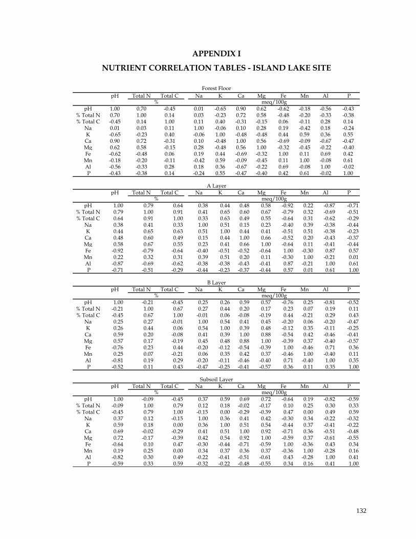
132 132
pH Total N Total C Na K Ca Mg Fe Mn Al P
pH 1.00 0.70 -0.45 0.01 -0.65 0.90 0.62 -0.62 -0.18 -0.56 -0.43% Total N 0.70 1.00 0.14 0.03 -0.23 0.72 0.58 -0.48 -0.20 -0.33 -0.38% Total C -0.45 0.14 1.00 0.11 0.40 -0.31 -0.15 0.06 -0.11 0.28 0.14
Na 0.01 0.03 0.11 1.00 -0.06 0.10 0.28 0.19 -0.42 0.18 -0.24K -0.65 -0.23 0.40 -0.06 1.00 -0.48 -0.48 0.44 0.59 0.36 0.55
Ca 0.90 0.72 -0.31 0.10 -0.48 1.00 0.56 -0.69 -0.09 -0.67 -0.47Mg 0.62 0.58 -0.15 0.28 -0.48 0.56 1.00 -0.32 -0.45 -0.22 -0.40Fe -0.62 -0.48 0.06 0.19 0.44 -0.69 -0.32 1.00 0.11 0.69 0.42
Mn -0.18 -0.20 -0.11 -0.42 0.59 -0.09 -0.45 0.11 1.00 -0.08 0.61Al -0.56 -0.33 0.28 0.18 0.36 -0.67 -0.22 0.69 -0.08 1.00 -0.02 P -0.43 -0.38 0.14 -0.24 0.55 -0.47 -0.40 0.42 0.61 -0.02 1.00
pH Total N Total C Na K Ca Mg Fe Mn Al P
pH 1.00 0.79 0.64 0.38 0.44 0.48 0.58 -0.92 0.22 -0.87 -0.71% Total N 0.79 1.00 0.91 0.41 0.65 0.60 0.67 -0.79 0.32 -0.69 -0.51% Total C 0.64 0.91 1.00 0.33 0.63 0.49 0.55 -0.64 0.31 -0.62 -0.29
Na 0.38 0.41 0.33 1.00 0.51 0.15 0.23 -0.40 0.39 -0.38 -0.44K 0.44 0.65 0.63 0.51 1.00 0.44 0.41 -0.51 0.51 -0.38 -0.23
Ca 0.48 0.60 0.49 0.15 0.44 1.00 0.66 -0.52 0.20 -0.43 -0.37Mg 0.58 0.67 0.55 0.23 0.41 0.66 1.00 -0.64 0.11 -0.41 -0.44Fe -0.92 -0.79 -0.64 -0.40 -0.51 -0.52 -0.64 1.00 -0.30 0.87 0.57
Mn 0.22 0.32 0.31 0.39 0.51 0.20 0.11 -0.30 1.00 -0.21 0.01Al -0.87 -0.69 -0.62 -0.38 -0.38 -0.43 -0.41 0.87 -0.21 1.00 0.61 P -0.71 -0.51 -0.29 -0.44 -0.23 -0.37 -0.44 0.57 0.01 0.61 1.00
pH Total N Total C Na K Ca Mg Fe Mn Al P
pH 1.00 -0.21 -0.45 0.25 0.26 0.59 0.57 -0.76 0.25 -0.81 -0.52% Total N -0.21 1.00 0.67 0.27 0.44 0.20 0.17 0.23 0.07 0.19 0.11% Total C -0.45 0.67 1.00 -0.01 0.06 -0.08 -0.19 0.44 -0.21 0.29 0.43
Na 0.25 0.27 -0.01 1.00 0.54 0.41 0.45 -0.20 0.06 -0.20 -0.47K 0.26 0.44 0.06 0.54 1.00 0.39 0.48 -0.12 0.35 -0.11 -0.25
Ca 0.59 0.20 -0.08 0.41 0.39 1.00 0.88 -0.54 0.42 -0.46 -0.41Mg 0.57 0.17 -0.19 0.45 0.48 0.88 1.00 -0.39 0.37 -0.40 -0.57Fe -0.76 0.23 0.44 -0.20 -0.12 -0.54 -0.39 1.00 -0.46 0.71 0.36
Mn 0.25 0.07 -0.21 0.06 0.35 0.42 0.37 -0.46 1.00 -0.40 0.11Al -0.81 0.19 0.29 -0.20 -0.11 -0.46 -0.40 0.71 -0.40 1.00 0.35 P -0.52 0.11 0.43 -0.47 -0.25 -0.41 -0.57 0.36 0.11 0.35 1.00
pH Total N Total C Na K Ca Mg Fe Mn Al P
pH 1.00 -0.09 -0.45 0.37 0.59 0.69 0.72 -0.64 0.19 -0.82 -0.59% Total N -0.09 1.00 0.79 0.12 0.18 -0.02 -0.17 0.10 0.25 0.30 0.33% Total C -0.45 0.79 1.00 -0.15 0.00 -0.29 -0.39 0.47 0.00 0.49 0.59
Na 0.37 0.12 -0.15 1.00 0.36 0.41 0.42 -0.30 0.34 -0.22 -0.32K 0.59 0.18 0.00 0.36 1.00 0.51 0.54 -0.44 0.37 -0.41 -0.22
Ca 0.69 -0.02 -0.29 0.41 0.51 1.00 0.92 -0.71 0.36 -0.51 -0.48Mg 0.72 -0.17 -0.39 0.42 0.54 0.92 1.00 -0.59 0.37 -0.61 -0.55Fe -0.64 0.10 0.47 -0.30 -0.44 -0.71 -0.59 1.00 -0.36 0.43 0.34
Mn 0.19 0.25 0.00 0.34 0.37 0.36 0.37 -0.36 1.00 -0.28 0.16Al -0.82 0.30 0.49 -0.22 -0.41 -0.51 -0.61 0.43 -0.28 1.00 0.41 P -0.59 0.33 0.59 -0.32 -0.22 -0.48 -0.55 0.34 0.16 0.41 1.00
APPENDIX I
NUTRIENT CORRELATION TABLES - ISLAND LAKE SITE
Forest Floor
A Layer
B Layer
Subsoil Layer
% meq/100g
% meq/100g
% meq/100g
% meq/100g
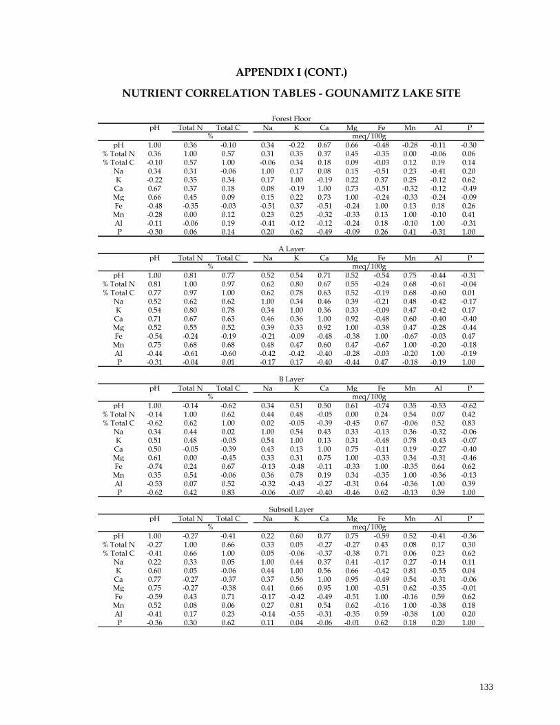
133 133
pH Total N Total C Na K Ca Mg Fe Mn Al P
pH 1.00 0.36 -0.10 0.34 -0.22 0.67 0.66 -0.48 -0.28 -0.11 -0.30% Total N 0.36 1.00 0.57 0.31 0.35 0.37 0.45 -0.35 0.00 -0.06 0.06% Total C -0.10 0.57 1.00 -0.06 0.34 0.18 0.09 -0.03 0.12 0.19 0.14
Na 0.34 0.31 -0.06 1.00 0.17 0.08 0.15 -0.51 0.23 -0.41 0.20K -0.22 0.35 0.34 0.17 1.00 -0.19 0.22 0.37 0.25 -0.12 0.62
Ca 0.67 0.37 0.18 0.08 -0.19 1.00 0.73 -0.51 -0.32 -0.12 -0.49Mg 0.66 0.45 0.09 0.15 0.22 0.73 1.00 -0.24 -0.33 -0.24 -0.09Fe -0.48 -0.35 -0.03 -0.51 0.37 -0.51 -0.24 1.00 0.13 0.18 0.26
Mn -0.28 0.00 0.12 0.23 0.25 -0.32 -0.33 0.13 1.00 -0.10 0.41Al -0.11 -0.06 0.19 -0.41 -0.12 -0.12 -0.24 0.18 -0.10 1.00 -0.31 P -0.30 0.06 0.14 0.20 0.62 -0.49 -0.09 0.26 0.41 -0.31 1.00
pH Total N Total C Na K Ca Mg Fe Mn Al P
pH 1.00 0.81 0.77 0.52 0.54 0.71 0.52 -0.54 0.75 -0.44 -0.31% Total N 0.81 1.00 0.97 0.62 0.80 0.67 0.55 -0.24 0.68 -0.61 -0.04% Total C 0.77 0.97 1.00 0.62 0.78 0.63 0.52 -0.19 0.68 -0.60 0.01
Na 0.52 0.62 0.62 1.00 0.34 0.46 0.39 -0.21 0.48 -0.42 -0.17K 0.54 0.80 0.78 0.34 1.00 0.36 0.33 -0.09 0.47 -0.42 0.17
Ca 0.71 0.67 0.63 0.46 0.36 1.00 0.92 -0.48 0.60 -0.40 -0.40Mg 0.52 0.55 0.52 0.39 0.33 0.92 1.00 -0.38 0.47 -0.28 -0.44Fe -0.54 -0.24 -0.19 -0.21 -0.09 -0.48 -0.38 1.00 -0.67 -0.03 0.47
Mn 0.75 0.68 0.68 0.48 0.47 0.60 0.47 -0.67 1.00 -0.20 -0.18Al -0.44 -0.61 -0.60 -0.42 -0.42 -0.40 -0.28 -0.03 -0.20 1.00 -0.19 P -0.31 -0.04 0.01 -0.17 0.17 -0.40 -0.44 0.47 -0.18 -0.19 1.00
pH Total N Total C Na K Ca Mg Fe Mn Al P
pH 1.00 -0.14 -0.62 0.34 0.51 0.50 0.61 -0.74 0.35 -0.53 -0.62% Total N -0.14 1.00 0.62 0.44 0.48 -0.05 0.00 0.24 0.54 0.07 0.42% Total C -0.62 0.62 1.00 0.02 -0.05 -0.39 -0.45 0.67 -0.06 0.52 0.83
Na 0.34 0.44 0.02 1.00 0.54 0.43 0.33 -0.13 0.36 -0.32 -0.06K 0.51 0.48 -0.05 0.54 1.00 0.13 0.31 -0.48 0.78 -0.43 -0.07
Ca 0.50 -0.05 -0.39 0.43 0.13 1.00 0.75 -0.11 0.19 -0.27 -0.40Mg 0.61 0.00 -0.45 0.33 0.31 0.75 1.00 -0.33 0.34 -0.31 -0.46Fe -0.74 0.24 0.67 -0.13 -0.48 -0.11 -0.33 1.00 -0.35 0.64 0.62
Mn 0.35 0.54 -0.06 0.36 0.78 0.19 0.34 -0.35 1.00 -0.36 -0.13Al -0.53 0.07 0.52 -0.32 -0.43 -0.27 -0.31 0.64 -0.36 1.00 0.39 P -0.62 0.42 0.83 -0.06 -0.07 -0.40 -0.46 0.62 -0.13 0.39 1.00
pH Total N Total C Na K Ca Mg Fe Mn Al P
pH 1.00 -0.27 -0.41 0.22 0.60 0.77 0.75 -0.59 0.52 -0.41 -0.36% Total N -0.27 1.00 0.66 0.33 0.05 -0.27 -0.27 0.43 0.08 0.17 0.30% Total C -0.41 0.66 1.00 0.05 -0.06 -0.37 -0.38 0.71 0.06 0.23 0.62
Na 0.22 0.33 0.05 1.00 0.44 0.37 0.41 -0.17 0.27 -0.14 0.11K 0.60 0.05 -0.06 0.44 1.00 0.56 0.66 -0.42 0.81 -0.55 0.04
Ca 0.77 -0.27 -0.37 0.37 0.56 1.00 0.95 -0.49 0.54 -0.31 -0.06Mg 0.75 -0.27 -0.38 0.41 0.66 0.95 1.00 -0.51 0.62 -0.35 -0.01Fe -0.59 0.43 0.71 -0.17 -0.42 -0.49 -0.51 1.00 -0.16 0.59 0.62
Mn 0.52 0.08 0.06 0.27 0.81 0.54 0.62 -0.16 1.00 -0.38 0.18Al -0.41 0.17 0.23 -0.14 -0.55 -0.31 -0.35 0.59 -0.38 1.00 0.20 P -0.36 0.30 0.62 0.11 0.04 -0.06 -0.01 0.62 0.18 0.20 1.00
% meq/100g
Subsoil Layer
% meq/100g
A Layer
% meq/100g
B Layer
Forest Floor
% meq/100g
APPENDIX I (CONT.)
NUTRIENT CORRELATION TABLES - GOUNAMITZ LAKE SITE