This PDF is a selection from an out-of-print volume from the National Bureau of

Economic Research

Volume Title: Annals of Economic and Social Measurement, Volume 5, number 1

Volume Author/Editor: Sanford V. Berg, editor

Volume Publisher: NBER

Volume URL: http://www.nber.org/books/aesm76-1

Publication Date: 1976

Chapter Title: Interpreting Spectral Analyses in Terms of Time-Domain Models

Chapter Author: Robert F. Engle

Chapter URL: http://www.nber.org/chapters/c10429

Chapter pages in book: (p. 89 - 109)

L

Annals of Economic and Soc in! Measurement, 5/1, 1976

INTERPRETING SPECTRAL ANALYSES INTERMS OF TIME-DOMAIN MODELS

BY ROBERT F. ENGL&

'This paper derives relationships between frequency-domain and standard time-domain distributed-lagand autoregressive mouin p-average models. These relations are well known in the literature but arepeesented here in a pedogogic form in order to facilitate interpretation of spectral and cros-sectralanalyses. in addition, the paper employs the conventions and discusses the estimationprocedures used inthe NBER's TROLL system.

I. INTROI)UC]ION

Although spectral analysis is a widely used tool in the statistical analysis of timeseries, the mathematical difficulties and the unfamiliarity of the concepts make itinaccessible to many economists. Increasing familiarity with time series modelssuch as distributed lags and autoregressive-moving average processes (so called"BoxJenkins" models), makes it now easy to describe and interpret spectralanalysis without the use of complicated mathematics. Traditional time domainand more difficult frequency domain (spectral) analysis are just two ways oflooking at the same phenomenon, but each has some advantages and the use ofboth can be an important aid in model building. Because frequency domainmethods ai'e more non-parametric, they are particularly useful in model specifica-tion.

The computational difficulties of performing spectral analysis have beensubstantially reduced through an innovative computer algorithm called the fastFourier transform and the availability of the NBER TROLL cotnputer systemthroughout the U.S. and many places abroad. The system is used by telephone andeasily performs both time domain and frequency domain analysis. All the facilitiesto he described in this paper are available in TROLL.

The paper is intended to be a tutorial. It will develop in Sections 2 and 3 thecorrespondences between time and frequency domain analyses assuming onlythat the reader is familiar with time domain analysis. A short description offrequency domain estimation in Section 4 focuses upon confidence intervals andsome adjustments which are available in TROLL. Finally, in Section 5, spectralanalysis is used to provide a guide to the specification of time domain models withan example from economics.

There are many excellent reference works on spectral analysis which shouldbe consulted for more details. Granger [6ff s perhaps the easiest to read, whileJenkins and Watts [10] is the most comprehensive. Fishman [7] focuses on someeconomic estimation problems and Dhrymes [3,4] extends this direction withsomewhat more mathematics. Hannan [8] gives a very rigorous treatment of the

* Research supported in part by National Science Foundation Grant Gi- II 54X3 to the NationalBureau of Economic Research, Inc.

t Parenthesized numerals refer to entries in the Reference section.

89

S

whole area. Relatively short and simple early expositions of the theory andpractice arc inien,kins[91 and Pazen[ 131 with a good application to economics inNeilove [12]. The book which is recommended as a companion to the TROLLsystem is Cooley, Lewis, and Welch [1] which is more application Oriented andwhich describes, in Chapters 5 and 7, the basic concepts used in designing thesystem. Also see Cooley, Lewis, and Welch [21.

2. THE SPECTRUM

Many data series can be considered successive chance observations over timecalled stochastic processes. Possibly, each observation is independent of thepreceding ones. However, for most applications, there is some suspected depen-dence between the observations. Both spectral analysis (frequency domain) andthe more familiar time domain analysis are ways to characterize this dependence.High correlations between neighboring observations or seasonal componentsmight be important forms of this dependence. Once the stochastic process ischaracterized, it may he possible to forecast its values, improve the efficiency of aregression where this is the disturbance, or make an inference about the economicmodel which produced such a variable.

Both frequency domain and time domain analyses begin with stochasticprocesses which are covariance stationary. This means that the covariancebetween an observation now and one a few periods later depends only on the timeinterval, not the dates themselves. Mathematically this can be expressed as(1) 'y(s) = E(x+, -- )(x, - /L)

where y is the autocovariance function and is the mean. The importantassumption is that neither depend upon 1. While this assumption may seem strong,it is because of this condition that information from the past can be used todescribe the present or future behavior.

Many economic time series appear to violate this assumption, particularlythose with pronounced trends. It is generally possible, however, to create anapproximately stationary series by taking first differences, or extracting a trend,thus leaving the series with a constant mean of zero. There may also be trends invariance which can often be removed by first taking logs of the series.

In the time domain the most common models are the autoregressive movingaverage models (ARMA). These may be purely autoregressive, purely movingaverage, or mixed.

A p-th order autoregressive and a q-th order moving average model aredefined in equations (2) and (3). respectively, while (4) is an ARMA (p. q).(2) x, = a1x,_1 +a2x,_2+. .

(2') A(L)x,(3) x, = bi_i +b2,_2+. . .+bqq +E,(3') x =(4)

(4') A(L)x B(L)e

90

In these equations E is a series of independent. identically distributed randomerrors with s, independent of x, for all i greater than zero; L is the lag operatorand A(L) and B(L) are polynomials. These classifications are not unique sinceoiie type of process can, in general, be transformed into another. Nevertheless,they provide useful, simple models of time series which can be tested with data orused for analysis. Knowledge of A(L) in (2'), B(L) in (3') or A (L) and 13(L) in (4')is equivalent to knowing the dynamics of the stochastic process of x.The spectrum provides another way of characterizing time series. In this casewe think of a series as being made up of a great number of sine and cosine waves ofdifferent frequencies which have just the right (random) amplitudes to make upthe original series. ThUS the list of how much of each frequency component wasnecessary is also a full description of the time series. The spectrum is a plot of thesquared amplitude of each component against the frequency of that component. Itis continuous and always greater than zero as long as there are no deterministicelements (that is, no exactly repeating components, or components which can bepredicted exactly on the basis of the past). This is a very general way to describe astochastic process.The spectral density function is defined as the Fourier transform of theautocovarjance function

(5) f(0)=y(0)+2 y(s)cOs(2w0s)= > y(s)e20s OO

where i = .1:1 e'° = cos (0)-f i sin(0), and the last equality follows from y(s) =y(s). There are several important features of this definition. First, althoughwritten in complex notation, the spectrum is real valued since all the imaginarysine terms cancel exactly. Second, since the cosine is symmetric f(0) = 1(1 - 0),and only the frequencies from 0 to 1/2 are needed to describe the spectrum.Third, integrating equation(S) from 0 to 1, shows that the area under the spectrumis equal to y(0), the variance. The spectrum is a decomposition of the variance intothe components contributed by each frequency. A strict proof of the probabilisticbasis of this interpretation is provided by the spectral representation theorem.Fourth, since 0 is measured in cycles per period, it appears that there are nocomponents from less than one cycle every two periods (the Nyquist frequency).The reason for this becomes clear upon reflection. When observing monthly data,weekly fluctuations will be indistinguishable from longer oscillations which havethe same value at the moment the observation is taken. The weekly componentwill therefore be counted with these lower frequencies.

To clarify the interpretation of a spectrum and help with the notion offrequency components, consider the spectrum in Figure 1 which has beenestimated from quarterly data.

From the definition of the spectrum in equation (5), the highest frequencyoscillation which can be distinguished is 0.5 cycle per period. At this frequency, ittakes two quarters to complete a cycle so there are two cycles per year. There is apeak at 0.25 cycle which corresponds to a four-quarter, or annual cycle. This ismost likely a seasonal component. Similarly, the peak at 0.5 also indicates aseasonal component since it has an even number of cycles per year. The peak at

91

/1/ Li

Figue I Typical spectrum

0.1 corresponds to a two and a half year oscillation. This might be a business cycleand economically interesting if it is significantly above its neighboring points.Generally, economic time series show behavior much like that of Figure 1.

The purpose of this paper is to emphasize the relationship between theseconcepts of frequency domain analysis and the more conventional time domainanalysis. The first order serial correlation coefficient is easily calculated in the timedomain and is generally large and positive for economic time series. This finding iseasily observed in the frequency domain as well. Multiply the spectrum bycos (2irO) and integrate to obtain from equation (5) just y(l), the first order serialcovariance. Roughly, this amounts to multiplying low frequencies by a positivenumber, high frequencies by a negative number, and adding. If the resuit ispositive, there is positive first order serial correlation. Thus data series withgenerally downward sloping spectra have positive first order serial correlationswhile those with upward sloping spectra have negative serial correlations. Veryimportant is the observation that spectra which are roughly symmetric about 0.25will show no first order serial correlation.

A useful application of this analysis is found in interpretation of regressionresults. The assumption of no serial correlation in the disturbance is equivalent tothe assumption that its spectrum is constant. The DurbinWatson statistic gives atest against the possibility that there is first order serial correlation. This is a testagainst a general slope of the spectrum of the disturbance, whereas one would liketo test against all forms of variation. In particular, notice that if the seasonality inFigure 1 were more severe, the spectrum might easily have no first order serialcorrelation but be far from constant. Durbin [5] formulated such a test based uponthe spectrum of the residuals. In general, examination of the residual spectrumgives very useful information about the validity of the regression assumptions.

The link between time domain and frequency donain is completed by aderiation of th' spectrum corresponding to the ARMA models of equations(2)(4). The basic result is quite simple but will be established in the appendix.

Lemma 1: If x is a stochastic process generated by the model

A(L)x, = B(L)c1

where e is a series of independent identically distributed random variables withvariance 0.2 and the polynomial A(L) has all roots outside the circle, then the

92

0 .25

'iththe

spectrum of x is given by

(6) f(0) = T2jB(z)/IA(z)I, 2 = e1 28)

Notice that z is a complex function of 0.Several examples should help to illustrate the usefulness of this result. First,notice that the spectrum of the very simple (white noise) process which has rio timedependence, is just a constant. It has equal contributions from all frequencies.Now consider the first order moving average process with parameter p.= r1+pr, . From equation (6) the spectrum of x is

f(0) = Ii +p °I2r2 = {1 +p2 + 2p Cas (2O)}2Evaluating this for U in the range (0, 1/2), gives a smooth spectrum which begins

le at (1 +p)2 and ends at (1 p)2. If p is positive, this has the typical spectral shapewhich is common to most economic time series, and which implies a positive serialcorrelation coefficient, p1(1 +p2). The first order autoregressive case is very

se similar but gives a somewhat steeper spectrum at low frequencies.in A very simple autoregressive model which captures the behavior of purely

seasonal stochastic processes for monthly data isis

From equation (6) the spectrum of this seasonal process is given byye h (0) 2/J 1 pe24"J2 = 21(1 + p2 - 2p cos (24ir0))

which is plotted in Figure 2. There are peaks at all the harmonic frequencies:0 = 1/12, 2/12, 3/12, 4/12, 5/12, 6/12, and all are equally important.

ry25

ontosaestike

1

in I+p2ial

S. Figure 2 Spectrum of pure seasonaly a

3. THE CROSS SPECrRUMnsx. The techniques used above can also be used to describe the relations between

two jointly covariance-stationary time series. Both the individual behavior andthe interrelations can be decomposed into basic sinusoidal elements.

The cross covariance function is a direct analogue of the autocovariancefunction. For two series with mean zero this is simply defined as:

y(s) E(x,,)'1)93

Again, notice that it does not depend on 1. The cross spectrum is similarly defined

as:

f(0) = .. y(s) C

Because 'y is no longer symmetric the cross spectrum is not a real valued tunct ionof 0 but rather a complex valued function.

Although the cross spectrum summarizes all the information in the series, itcannot be plotted directly. Instead, one examines statistics called "coherencesquared," "gain," and "phase." These measures are defined here and given arather extended interpretation below, connecting these concepts with the ideas ofdistributed lag regression models.

The coherence squared (COH) is like a correlation coefficient and is definedas:

COH(0) = If(0)I2/f(0)fy(0)

which is clearly between 0 and 1.The gain (G) indicates how much the spectrum of x has been amplified to

approximate that component of y.

G(0) = f1(0)IIf(0)This expression can clearly never be negative. However, if it is small, it indicatesthat at frequency 0, x has little effect on y.

The phase (PH) is a measure of the timing between the series. It is measuredin the fraction of a cycle that y leads x.

'ImPH(0)=arctan ( Re(f(0)) /

where Im and Re are the imaginary and real parts of the cross spectrum.* There isa natural ambiguity about the phase since adding or subtracting I whole cyclefrom an angle will not change its tangent. The phase is known only up to adding orsubtracting an integer and therefore even the lead-lag relation is not known forsure. The plot of the phase is designed to emphasize this fact. It is possible tocombine the phase and the gain in a simple expression

f(0)/f(0) =G,(0) e_itPe)

Two other potentially useful measures of the cross spectrum are its amplitude, which is merely its absolute value, and its time lag. The latter describes thephase in terms of the number of periods y leads x rather than the fraction of acycle. Although this seems like a useful measure, the natural ambiguity of thephase also makes the time lag ambiguous and difficult to interpret. This may not bethe case at low frequencies. where these difficulties are less likely to be important.

* The appropriate quadrant for PH is chosen on the basis of the signs of the real and imaginarYcomponents of the cross spectrum.

94

A natural and very general WilY for economists to think about the relationsbetween two time series is in terms of a hivariate distributed lag model, such as

Y1ivx1.,+1.

This is often rewritten in terms of the lag operator L as

y, => w1L.'x,+u = w(L)x,+ r,

where, for generality, leads as well as lags have been allowed and U' isinterpreted as a lead operator. The same techniques required for equations (5)and (6), establish frequency domain interpretations of equation (14).Lemma 2: If y is generated by a distributed lag model

y = w(L)x +where x and E are uncorrelated covariance stationary processes, then

Y (0)= w(z ')f(0),and

f(9) w(z)I2f(o) +f(0)where z = 2rn0)

Notice from (16) that the variancc of y is broken into two parts: one which isthe variation due to x modified by the lag distribution and the other due to thedisturbance. Equation (15) shows that f/f is an estimator of w(z) which is just afunction of the lag coefficients. Once w(z) is known, all the lag coefficients can befound by merely taking the inverse Fourier transform. This is the basis of a veryuseful type of distributed lag estimation which is often called Hannan's inefficientmethod.*

Now consider running a regression of one component of y against the samefrequency component of x. The regression coefficient would be the ratio of thecovariance of x and y to the variance of x. In spectral notation this would be justf(0)/f(0). The R-squared of this regression is one minus the unexplainedvariance over the total variance. Substituting (15) into equation (16) demonstratesthat the coherence squared is just the R-squared of this regression.

Similarly, from (12), the regression coefficient is the gain times e2''°. Theregression coefficient is just the gain if there is no time lag betweerm the indepen-dent and dependent variables. If there is a time lag, the gain can be interpreted asthe regression coefficient if the series were lagged just the right amount toeliminate any phase shift, and the phase is the angle by which they would have tobe shifted (Or the phase over the frequency is the time shift which is necessary). Asa particular example, if the series are negatively related, the gain will still bepositive but the phase will be 0.5.

* It is inefficient because it does not use the ploperties of the disturbance to construct an estimatorwith the smallest possible variance. It too is available in TROLL.

95

ae

I

in summary, the coherence squared, the gain and the phase at a particularfrequency can be interpreted in terms of a regression using only data at thatfrequency. The coherence squared is the R2, the gain is the regression cocfficjtonce any delay has been eliminated, and the phase is the angular shift needed tomake this delay.

From Lemma 2 it is simple to plot the gain and phase corresponding to anyparticular time domain distributed lag model. A variety of these plots, often caVedBode plots. are presented in Figure 3. In the balance of this section these figureswill be analyzed for salient characteristics; and in Section 5 these are used to helpspecify a distributed lag model.

ho

I. Simple Siasic Model

n(L) = to

w(: I) =

G(0) = 'to

PH(0) = 0

0

2. Simple Delay

w(6) =

w(z 1) =

0(0) =

PH(0)=

I

0

0

96

PHII.

PH

I6

G

WI

t

dCs

'pI40 + w1

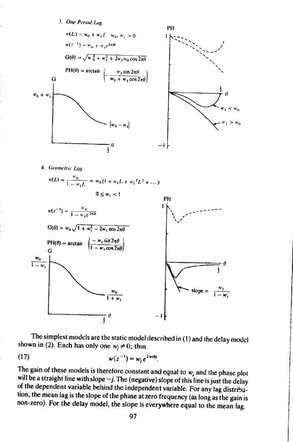
3. One Period Lag

'v(L) = w0 + Wi!. ii., W > 0

14(7 - )

0(0) .,Jn +

w(z) = I - Ii'1e

I

4. Gt'oyneirjc Lag

(L) 11(1

(I + w1 L +1 +-. III!.

0

W0

G(0) = wos/iwf - 2w cos2ft0

wo

I -f w1

PH

, 0

<

It >

The simplest models are the static model described in (1) and the delay modelshown in (2). Each has only one 0; thus(17) w(z)= ie210'.The gain of these models is therefore constant and equal to w1 and the phase plotwill be a straight line with slope j. 'The (negative) slope of this line isjust the delayof the dependent variable behind the independent variable. For any lag distribu..tion, the mean lag is the slope of the phase at zero frequency (as long as the gain isnon-zero). For the delay model, the slope is everywhere equal to the mean lag.

97

PH(0) = arctan w1 sin 2n0G w0+w1os/

PH(0) arctan

G

j - W1 Sifl 2,tOs-

10

I4'O - 111 I

2w

Wo + Ict

U

6. Four Period Differences

w(L) w0(I - L4)

= w0(i -

G(6) = - 2cos(SnO)

I sinSnU/PHw) = arcian ! II cos8tOI

()

Models (3) and (4) include current and one lagged independent variable, anda lagged dependent variable, respectively. These very common types of lagdistributions are used to model processes where the dependent variable OnlY

adjusts partially to a change in the independent variable in the current period. In

model (3) the adjustment is completed in the second period, while in model (4) it

continues forever but with geometrically declining effect.In both of these cases, the gain is largest at low frequencies and then falls at

higher frequencies. At zero frequency z = 1 and the gain is the sum of the lag

coefficients or the long run propensity. Since z cannot exceed one, the peak of the

98

P11

0

I,'-.-.-.-.V - - -

PH

Hrsf DiIbrefllec

w(L) w1L W1 > 0

w(z') = Wo -

0(0) = /w0 CQS2IIO

- w1 sin 2n0PH(0) = arcian I -- , cos 21) /

0

andlag

onlydin(4) it

ails ate lagof the

gain function will always be at zero frequency if all the ta weights are positive.The phase will he zero at zero frequency and then will decline with a slope equal to(minus) the mean lag. For more complicated models with all positive lag weights,the phase may change sign for higher frequencies; nevertheless, the initial slopewill be the mean lag.The final two models have a different charactei. In these cases, the dependent

variable is influenced by the rate of change of the independent variable; the lagweights change sign. The peak in the gain function can 110W occur at anyfrequency, but it will generally not be at Zero. In fact, if the sum of the lag weightsis zero as with first differences, the gain will be zero at the beginning. Notice theinteresting double peak associated with a four period difference. A twelve perioddifference would of course have six peaks and a three period difference wouldhave one and a half (the second peak would occur at 0 = 0.5).

The phase plots can have both positive and negative portions. If the gain isnon-zero at the origin, then the slope of the phase at the origin will be algebraicallyequal to (minus) the mean lag of the distribution. But, the mean lag is not a usefulmeasure when the lag weights are of different signs. En particular, a negative meanlag does not imply a lead.

Both plots can be constructed for many other lag distributions either by handor using the computer. A simple corollary of Lemma 2 will make it easy tocombine these simple forms into more complicated lag distributions.

corollary. If a lag distribution can be written as the product of two lagdistributions such as

thenw(L) u(L)v(L),

G(0) = Gj0)G,(o)

PH(0) PH(8) + PH0(0).

The rule for combining lag distributions is that the gains multiply and thephases add. A special case of this is familiar from the time domain: the product oftwo lag distributions will have a long run propensity which is the product of theseparate propensities and a mean lag which is the sum.

As an example, consider the geometric form when the independent variableis lagged two periods. This is the product of a two period de!ay and a laggeddependent variable. Thus the gain is the product of a constant and the geometricgain, while the phase is the sum of the constant slope of the delay and the variationshown for the geometric.

4. SPECTRUM ESTIMATtON

There are several distinct methods for estimating spectra and cross-spectra.The advantages and disadvantages of each have been extensively discussed. inparticular, see Cooley, Lewis, and Welch [1] and Parzen [14]. Since the rediscov-ery of the fast Fourier transform, computational considerations suggest thatperiodograni averaging may be the most efficient method for spectrum estimation.In addition, it is conceptually simplest and leads to great versatility in the

99

j

estimation procedures. Finally, the usefulness of the periodograrn in regression

and various test pioceclures makes it sensible to Compute this as a first Step See

also Jones [111 and Tick [1 5]The periodogram is defined as the square of the absolute value of the Fourier

transform of the data series at each frequency, all divided by in, the number ofobservations. The formula for the periodogram is

rn-I 2

x,e 2wril,

in I

where 01j/rn and j.=0, 1, 2, .. .,rn. This quantity is an estimator of thespectrum, but it is not a very good one. The expected value of the periodogram is

rn-I ( -E(I(O1)) =

m Vy(v) e2°'.

= -rn4- I

For large values of in this estimator is art unbiased estimator of the spectrum, since

'y(v) is small for large v. Unfortunately, it is not a consistent estimator since thevariance does not decrease as the sample approaches infinity. In fact, theperiodogram at each frequency is approximately proportional to a chi squaredrandom variable with two degrees of freedom, regardless of the number ofobservations. An intuitive explanation for this unusual circumstance is that as thesample becomes larger, more and more frequency points are estimated ratherthan obtaining better estimates of a fixed number of parameters. This explanationalso suggests the solution. The average of a few neighboring points should give abetter estimate of the spectrum in that neighborhood. Thus smoothing proceduiesmust be used to obtain consistent spectrum estimators.

Two averaging or smoothing procedures, called "windows", are commonlyused with periodogram averaging. A rectangular moving average gives theminimum variance for smoothing over a flat spectrum using only a certain numberof points. However, when there are peaks in the spectrum, the rectangularwindow will lead to considerable bias and broadening of the peaks. An alternativewindow is a triangular window which gives the spectrum a much smootherappearance and is often better at describing the shape of peaks.

The width of the window is an important parameter in the estimation. Thewider the window, the smaller is the variance of the resulting estimate; yet, thewider the window, the more serious may be the bias of smoothing over non-smooth portions of the spectrum. Two measures of width can be used to describethe windows, the bandwidth and the range. The bandwidth is the half-power widthof the window. It is measured in frequency units, i.e., it is a fractional number ofcycles per period. if, for example, the bandwidth is specified as 0.1, there will befive separate "bands" since the frequencies range from 0 to 0.5. For manypurposes, spectral estimates separated by more than one bandwidth arc consi-dered to he independent.

The second measure is the range. This is merely the number of spectral pointsused in each moving average; it gives the separation between which two points areknown to be completely independent, lithe effective sample is 200 observationS(implying 100 points in the spectrum) and the range is 20, there will be five

100

F

r

e

h

fC

ts

C

S

separate window widths in the estimation A sensible value foi the range is v,where m is the number of observationsNear the endpuints of the spectrum, the smoothing procedures must bemodified. One choice is to decrease the range so that the window does not Overlapthe endpoints. Because the variance increases as the window becomes nat-rower,the variance increases markedly at very low or very high frequencies and one musthe very cautious in interpreting low frequency peaks or troughs.An alternative endpoint procedure is to keep the range constant but takeadvantage of the symmetry properties of the spectrum. The smoothing windowswill "wrap" around the endpoints of the spectrum since the spectrum at +0 is justthe same as at 6. This method will give smaller variances but bigger biases thanthe first method.The spectral estimator resulting from smoothing the periodogram is approxi-mately proportional to another chi squared random variable, this time with moredegrees of freedom. The equivalent degrees of freedom are equal to

(20)

where B is the bandwidth. This allows Computation of a confidence interval for thespectrum. On the spectral plot, a 95 percent confidence interval can he con-structed for each frequency separately.Estimates of the cross spectrum arc accomplished in exactly the samemanner. The finite Fourier transform of one series is multiplied by the complexconjugate of the Fourier transform of the other to form the cross periodogram.The real and complex parts of this are then smoothed individually, just as for theperiodogram. The sampling distributions for the various measures derived fromthe cross spectrum also depend only on the equivalent degrees of freedom of theestimate. With the coherence plot, the critical point for a 5 percent test of thehypothesis of zero coherence can be calculated. Approximate 50 percent confi-dence intervals for the gain can be plotted with the output. These depend on thesample coherence; where the coherence is small, the confidence interval is large.

When using a wide window, peaks tend to be spread out. For many series weknow a priori where these peaks will be, either because the series is typical inhaving strong low frequencies or because it has important seasonality. In thesecases "prewhitening" is often recommended. This amounts to dividing the rawperiodogram by the expected or typical shape, smoothing this "prewhitened"periodogram which no longer has the large peaks, and then "recoloring" bymultiplying by the typical spectral shape. A seasonal and non-seasonal version ofthe Prewhitening filter might he important. Prewhitening can be done in connec-tion with either spectrum or cross spectrum estimation,

A second characteristic which is likely to make the smoothing procedurebadly biased in cross spectral estimation is misalignment of the series. When OflCseries lags another by several periods, there is a peak in the cross covarlancefunction which is not at zero. This leads to a regular oscillation in the amplitude ofthe cross periodogram. Smoothing this will obscure this particular bit of informa-tion as well as distorting other results. The recommended procedure is to firstdivide the cross periodogram by an aligning series, smooth the COSS periodogram,and then remultiply it by the aligning series. To construct the alignment series one

101

I,) first computes the inverse lourier transform of the cross periodogram which isexactly the cross covariancc function. This could have been computed from thedata directly, hut such a method is apparently iii1ciii. to the cuillputalion 0,Fourier arid inverse Fourier transforms. Searching the cross covariance functionfor the maximum yields the information needed to construct the alignment series.If this procedure were applied to the estimate of the spectrum or a cross spectnmwhich was already aligned, the maximum covariance would be the zeroth estimateand thus the alignment series would be unity and would have no effect.

The Fourier transform algorithm used in these computations is the Cooley-Tukcy fast Fourier trahsform. En its basic form it expects a series with 2" elementsand thus each series is padded out to this length with zeros (the mean). Thenumber of spectral points estimated is therefore 2" which arc evenly spacedbetween the frequencies U and 1/2 cycle per basic time unit of the data.Frequently it is desirable to estimate the spectrum at particular points or not topad with zeros. in this case, ii is possible to pick an integer so that the series ispadded to N 2'r. Choosing r = 3. for example. would insure factors of 12 whichwould he required in order to have exact seasonal points with monthly data. Thisvariation can make substantial difference in the results when there is strongseasonality.

5. Ti-rn tJsr of: SPECFRA IN SI'ECIFYING Mol)Ers

This paper has shown that the time domain and the frequency domain are justtwo different ways of looking at the same models. 'the estimation procedures are,however, dramatically different, and it is here that the two techniques canfruitfully be combined. In order to estimate an ARMA or a distributed lag model,using time domain methods, one must first specify (or "identify" as the statisticians say) the form of the model. The process of specification usually involves aseries of trial forms and statistical tests coupled with a liberal amount of goodjudgment. The judgment is particularly important since the tests become ofquestionable validity when applied in sequence.

On the other hand, the spectral methods do not require the specification ofthe model. The estimation procedure is independent of the form of the model.This is clearly an advantage since the first difficult step can he avoided; however, itis also a disadvantage, since in general, a very large number of parameters must beestimated and will have relatively wide confidence intervals.

The situation is exactly comparable with the choice of parametric or non-parametric statistical methods. If the parameterization is correct, the parametricprocedure is far more efficient than the non-parametric procedure. 1-lowever, ifthe parameterization is incorrect, only the non-parametric method will give avalid result. The user of non-parametric statistics gives up some efficiency forinsurance against a wrong pararncterization.

This discussion suggests a two step procedure for the analysis of stochasticprocesses. Use the spectral methods to aid in the specification of time domainmodels, and then use standard time domain methods to estimate them, therebyavoiding the trial and error search for an appropriate model. This is an approachwhich has been used by engineers for many years but has not had wide acceptance

102

justare.candel,

tisti-es a

goode of

on ofodd.er,itst be

non-.etricer, iflye a

cy for

hastiComainerebyroach

ptaiICe

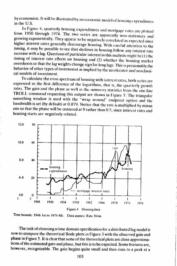
by economists. It will be illustrated by an CCOI1OJfl!C model ot housing expendituresiii the U.S.Iii Figume 4, quarterly housing expenditures and nlOrtgage rates are plottedfrom 1950 through 1974. The two series are apparently flOn-Stationjry and

growing exponentially. They appear to be negatively correlated as expected sincehigher interest rates generally discourage housing. With careful attention to thetiming, it may be possible to see that declines in housing follow any interest rateincrease with a lag. Questions of particular interest in this analysis might he (lithetiming of interest rate effects on housing and (2) whether the housing marketovershoots so that the lag weights change sign for long lags. This is presumably thebehavior of other types of investment as implied by the accelerator and neoclassi-cal models of investment.

To calculate the cross spectrum of housing with interest rates, both series areexpressed as the first diljerence of the logarithms, that is, the quarterly growthrates. The gain and the phase as well as the summary statistics from the one lineTROLL command requesting this output are shown in Figure 5. The triangularsmoothing window is used with the "wrap around" endpoint option and thebandwidth is set (by default) at 0.079. Notice that the rate is multiplied by minusone so that the phase will be centered at 0 rather than 0.5. since interest rates andhousing starts are negatively related.

I 2 1 I I

1946 1950 1954 1958 1962

Figure 4 Housiiig data

Time bounds: 1946 1st to 1974 4th. Data names: Rate Fious.

The task of choosing a time domain specification fora distributed lag model isnow to compare the theoretical Bode plots in Figure 3 with the observed gain andphase in Figure 5. It is clear that none of the theoretical plots are close approxima-tions of the estimated gain and phase, but this is to be expected. Some features are,however, recognizable. The gain begins quite small and then rises to a peak at a

1966 1970 1974 1978

103

:

housing

- Interest rates

12.0 80

10.0 60

8.0 40

6.0 20

4.0 0

ishe

onCs.urnate

ey-ntshe

cedata.t tos isich

['hisong

0.000.000

0.60

0.00

0.60

1.30

Summary statistics anti uptions:Type of smoothing: Wrap-triangular. Range: 10.Type of prewhitening: None.FET parameter: 1.Preprocessing: Demean.Number of observations in data series: 100Basis: 128.Bandwidth: 0.079.No alignment.Critical coherence squared tat 5 percent level): 0.636.-. (Del( 1: Log(Rate))) variance: 0.001. Spectrum total: 0.001.DeI(1 : Log(Hous)) variance: 0.003. Speclrum total: 0.003.

Figure 5 Gain and phase between housing and interest rates

period of about 10 quarters where the interest rate elasticity is almost 2. Thesecond most important peak is at approximately 2 quarters per cycle. These lookroughly like the four quarter first difference except that the second peak is at toohigh a frequency and is too small. The phase looks much like a OflC quarter delayfor the first half of the spectrum but then deviates from this in the second half.

104

((.00

0.000 0.100

0. 00

I I I0.200

GAIN

PHASE

L__L.___.. I I I I J__L...L_L_.((3011 0.41(t) 0.500

0.300 0.400 0.51)0

IL,

R R1

R4

Con

si.

(100

0.50

00.

000

0.10

00.2

00 0

.300

-1.

00

-0.5

0-1

.00

-0.2

00.

000

0.10

0 0.

200

0.30

0 0.

400

0.50

000

00 0

.100

0.0

0 0.

1*)

0.40

0 0.

111

0.lY

0.10

0 0.

10)

:.sta

tisc.

cs in

par

enth

eses

. All

regr

essi

ons

have

98

obse

rvat

ions

.

TA

BLE

IR

EG

RE

SS

ION

CO

EF

FIC

IEN

TS

FO

R H

OU

SIN

GA

ND

INT

ER

ES

T R

AT

ES

.17

(1.2

8).5

5(3

.75)

.22

(1.3

6).1

6(1

.10)

.0(2

.19)

.42%

2.4

0092

.69

(6.7

1)-

.07

(.58

)-

.12

(1.1

8).2

6(1

.94)

3600

4.5

2049

.5!

(4.8

6).0

31.

23)

.16

(1.6

0).0

8(.

60)

.62

(411

).1

5(.

91)

.05

(.32

).0

8(.

52)

.01

(2.2

9)

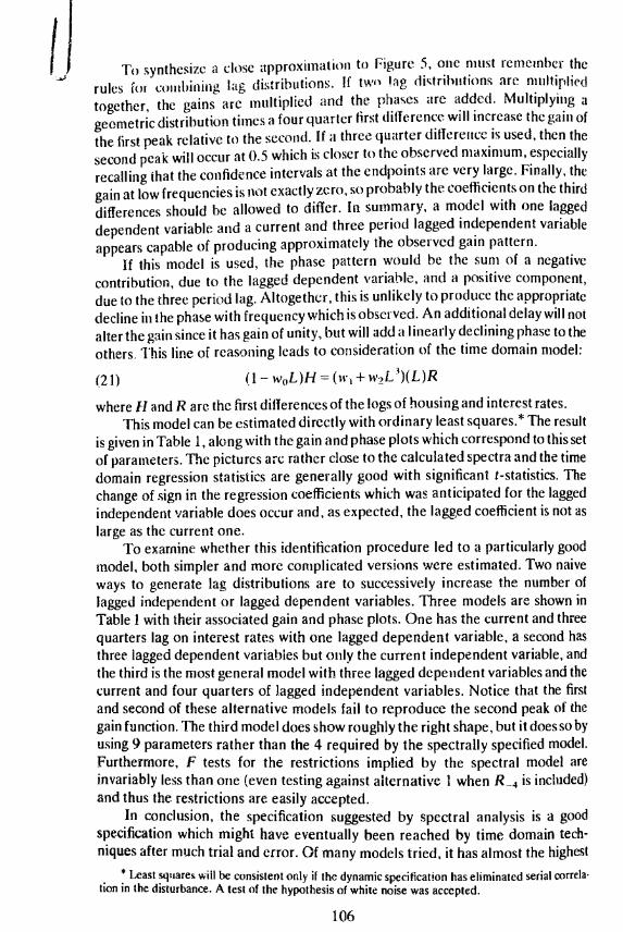
Li To synthesize a ckse approximation to Figure 5, One must remember therules t( combining lag distributions. If twn !ag distributions are niultipliedtogether, the gains are multiplied and the phases are added. Multiplying ageometric distribution times a four quarter first difference will increase the gain ofthe first peak relative to the second. If a three quarter difference is used, then thesecond peak will occur at 0.5 which is closer to the observed maximum, especiallyrecalling that the confidence intervals at the endpoints are very large. Finally, thegain at low frequencies is not exactly zero, so probably the coefficients on the thirddifferences should he allowed to differ. In summary, a model with one laggeddependent variable and a current and three period lagged independent variableappears capable of producing approximately the observed gain pattern.

If this model is used, the phase pattern would be the sum of a negativecontribution, due to the lagged dependent variable, and a positive component,due to the three period lag. Altogether, this is unlikely to produce the appropriatedecline in the phase with frequency which is observed. An additional delay will notalter the gain since it has gain of unity, but will add a linearly declining phase to theothers. This line of reasoning leads to consideration of the time domain model:

(21) (1 WOL)H (t1 + w,L)(L)R

where H and R arc the first differences of the logs of housing and interest rates.This model can be estimated directly with ordinary least squares.* The result

is given in Table 1, along with the gain and phase plots which correspond to this setof parameters. The pictures arc rather close to the calculated spectra and the timedomain regression statistics are generally good with significant t-statistics. Thechange of sign in the regression coefficients which was anticipated for the laggedindependent variable does occur and, as expected, the lagged coefficient is not aslarge as the current one.

To examine whether this identification procedure led to a particularly goodmodel, both simpler and more complicated versions were estimated. Two naiveways to generate lag distributions are to successively increase the number oflagged independent or lagged dependent variables. Three models are shown inTable 1 with their associated gain and phase plots. One has the current and threequarters lag on interest rates with one lagged dependent variable, a second hasthree lagged dependent variables but only the current independent variable, andthe third is the most general model with three lagged dependent variables and thecurrent and four quarters of Jagged independent variables. Notice that the firstand second of these alternative models fail to reproduce the second peak of thegain function. The third model does show roughly the right shape, but it does so byusing 9 parameters rather than the 4 required by the spectrally specified model.Furthermore, F tests for the restrictions implied by the spectral model areinvariably less than one (even testing against alternative 1 when R4 is included)and thus the restrictions are easily accepted.

In conclusion, the specification suggested by spectral analysis is a goodspecification which might have eventually been reached by time domain tech-niques after much trial and error. Of many models tried, it has almost the highest

* Least squares will be consistent only ii the dynamic specification has eliminated serial correla-tion in the disturbance. A test of the hypothesis of white noise was accepted.

106

corrected R2 and F tests supported the restrictions it imposed. The econonhicresult is thit there appears to be a one quarter delay before interest rates influencehousing, thereafter there is a geometrically declining effect. Eventually (one yearlater) there is a change in the diteetion of housing response as the market haspresumably caught up to the desired capital stock. This is easily seen in the timedomain but is also apparent in the frequency domain since the gain is small for lowfrequencies.This example lends credibility to the proposition that the use of both time andfrequency domain techniques may enrich each and, in particular, that frequencydomain methods may be very helpful in model specification

received April 1974 NBER and University of california, San Diegorevised May 1975

APPENDIX

Lemma A. 1: If x is a stochastic process generated by the model= B(L)e,

where r is a series of independent identically distributed random variables withvariance o2, arid 4(L) has all roots outside the unit circle, then the spectrum of xis given by

LW) = u2IB(z)I2/jA(z)I2where z (-2irO)

Proof: Consider the moving average processq

=I = U

where the e are all independent. Then

y(s)=Ex1+x1=Ej=() k=()

where the expectation on the right only has non-zero values where k = si and0< k q. Therefore for q s

and is 0 otherwise. The spectrum of x is defined using equation (5) and thesymmetry of y by

f(0) y(s)z=q

=0' ± b1b..5(z+z)+u2 bs= I J5 1=0

107

r

/1 which can be written

f(0)u2 h7' I)Z '

There is nothing in this proof which requires that q he finite. Since every stableARMA process has a (possibly infinite dimensional) moving average representa-tion, the result is true for any ARMA process.

Lemma A.2: If y is gcnerated by a distributed lag model

y=w(L)x+

where x and e are uncorrelated covariance stationary processes, then

f>.(0) w(z 5f(o)

f,(0) = Iw(z)I2f(0) +f, (0)and

where zfr2inO>

Proof: Without loss of generality take both x and y to have mean zero

'y(s) Ex14

=E w,x: jxr+, +Ex44E,

yy(S)r w,y(s+j)

y,(s)z5 w1y(s+j)z'z'

= w1z'f(0)

f1(0) w(z')f(0).And

y(s) = Ey145y,

= E( w1x4_1 + e5)( WkX1k + e,)

y(s)= W1Wky(sj+k)-t--y(s)

f(0)= y(s)z5

w1w',(sj+k)f 4k -k j $z z + y1(s)z

w1z

f(6)= Iw(z)I2f(0)'f(0).

108

I

REFERENCES

[II Cooley, J. W., P. A. W. Lewis, and P. 1). Wekh, The Fast Fourier Transform Algorithm and its/tppliccuions, IBM Research Paper RC 1743, t67.

[2] "The Application of the Fast Fourier Transform Algorithm to the Estimation of Spectraand Cross Spectra," Journal of Sound Vibrations, 1970.Dhrymes, P. J., Econometrics: Statistical Foundations and Applications. New York: Harper andRow, 1970.

Distributed Lags, Problems of Estimation and Formulation. San Francisco: 1-lolden Day,1971.Durbin, J., "Tests for Serial Correlation in Regression Analysis Based on the Periodogram ofLeast Squares Residuals," Biometrica, 56(1969), pp. 1-14.Granger, C. W. J., in association with M. Hatanaka, SpectralAnalysis of Economic Time Series.Princeton: Princeton University Press, 1964.Fishman, G. S., SpectralMethods in Econometrics. Cambridge: Harvard University Press, 1969.

[81 Hannan, E. I., Multiple 'flme Series. New York: J. Wiley, 1970.Jenkins, G. M., "General Considerations in the Analysis of Spectra," Technomeirics, 3,2 (1961),pp. 133-166.Jenkins, 0. M. and D. G. Watts. Spectral Analysis and Its Applications. San Francisco: HoldenDay, 1969.

[ii] Jones, R. H., "A Reappraisal of the Perioclogram in SpecOal Analysis," Technometrics, 7(1965),pp.53I-542.

t12] Nerlove, M., "Spectral Analysis of Scasonal Adjustment Procedures," Econometrica. 32 (July1964), pp. 241-286.

[131 Parzen, E., "Mathematical Considerations in the Estimation of Spectra," Technometrics, 3, 2(1961), pp. 167-190.-. "Multiple Time Series Modeling." in Multivariate Analysis. P. Kr'shnaia editor. NewYork: Academic Press, 1969.Tick, L. H., Letter to the Editor, Technornetrics, 8(1966), pp. 559-561.

109

S