Atmos. Chem. Phys., 16, 7285–7294, 2016www.atmos-chem-phys.net/16/7285/2016/doi:10.5194/acp-16-7285-2016© Author(s) 2016. CC Attribution 3.0 License.

Interpreting space-based trends in carbon monoxide withmultiple modelsSarah A. Strode1,2, Helen M. Worden3, Megan Damon2,4, Anne R. Douglass2, Bryan N. Duncan2, Louisa K. Emmons3,Jean-Francois Lamarque3, Michael Manyin2,4, Luke D. Oman2, Jose M. Rodriguez2, Susan E. Strahan1,2, andSimone Tilmes3

1Universities Space Research Association, Columbia, MD, USA2NASA Goddard Space Flight Center, Greenbelt, MD, USA3National Center for Atmospheric Research, Boulder, CO, USA4Science Systems and Applications, Inc., Lanham, MD, USA

Correspondence to: Sarah A. Strode (sarah.a.strode@nasa.gov)

Received: 28 January 2016 – Published in Atmos. Chem. Phys. Discuss.: 2 February 2016Revised: 24 May 2016 – Accepted: 26 May 2016 – Published: 10 June 2016

Abstract. We use a series of chemical transport model andchemistry climate model simulations to investigate the ob-served negative trends in MOPITT CO over several re-gions of the world, and to examine the consistency of time-dependent emission inventories with observations. We findthat simulations driven by the MACCity inventory, used forthe Chemistry Climate Modeling Initiative (CCMI), repro-duce the negative trends in the CO column observed byMOPITT for 2000–2010 over the eastern United States andEurope. However, the simulations have positive trends overeastern China, in contrast to the negative trends observed byMOPITT. The model bias in CO, after applying MOPITTaveraging kernels, contributes to the model–observation dis-crepancy in the trend over eastern China. This demonstratesthat biases in a model’s average concentrations can influencethe interpretation of the temporal trend compared to satelliteobservations. The total ozone column plays a role in deter-mining the simulated tropospheric CO trends. A large pos-itive anomaly in the simulated total ozone column in 2010leads to a negative anomaly in OH and hence a positiveanomaly in CO, contributing to the positive trend in simu-lated CO. These results demonstrate that accurately simulat-ing variability in the ozone column is important for simulat-ing and interpreting trends in CO.

1 Introduction

Carbon monoxide (CO) is an air pollutant that contributesto ozone formation and affects the oxidizing capacity of thetroposphere (Thompson, 1992; Crutzen, 1973). Its primaryloss is through reaction with OH, which leads to a lifetimeof 1–2 months (Bey et al., 2001) and makes CO an excel-lent tracer of long-range transport. Both fossil fuel com-bustion and biomass burning are major sources of CO. Thebiomass burning source shows large interannual variability(van der Werf et al., 2010), while fossil fuel emissions typ-ically change more gradually. The time-dependent MACC-ity inventory (Granier et al., 2011) shows decreases in COemissions from the United States and Europe from 2000 to2010 due to increasing pollution controls but increases inemissions from China. MACCity emissions for years after2000 are based on the Representative Concentration Path-way (RCP) 8.5 (Riahi et al., 2007). The REAS (Kurokawaet al., 2013) and EDGAR4.2 (EC-JRC/PBL, 2011) inven-tories also show increasing CO emissions from China. Thebottom-up inventory of Zhang et al. (2009) shows an 18 %increase in CO emissions from China from 2001 to 2006, andZhao et al. (2012) estimate a 6 % increase between 2005 and2009. However, there is considerable uncertainty in bottom-up inventories, and comparison of model hindcast simula-tions driven by bottom-up inventories with observations pro-vides an important test of the time-dependent emission esti-mates.

Published by Copernicus Publications on behalf of the European Geosciences Union.

7286 S. A. Strode et al.: Interpreting space-based trends in carbon monoxide with multiple models

Space-based observations of CO are now available for overa decade and show trends at both hemispheric and regionalscales. Warner et al. (2013) found significant negative trendsin both background CO and recently emitted CO at 500 hPaover southern hemispheric oceans and northern hemisphericland and ocean in Atmospheric Infrared Sounder (AIRS)data. Worden et al. (2013) calculated trends in the CO col-umn from several thermal infrared (TIR) instruments includ-ing MOPITT and AIRS. They found statistically significantnegative trends over Europe, the eastern United States, andChina for 2002–2012. He et al. (2013) also report a negativetrend in MOPITT near-surface CO over western Maryland.

Surface concentrations of CO show downward trends overthe United States driven by emission reductions (EPA, 2011),consistent with the space-based trends. Decreases in the par-tial column of CO from FTIR stations in Europe also showdecreases from 1996 to 2006, consistent with emissions de-creases (Angelbratt et al., 2011). Yoon and Pozzer (2014)found that a model simulation of 2001 to 2010 reproducednegative trends in surface CO over the eastern United Statesand western Europe, but showed a positive trend in surfaceCO over southern Asia.

The cause of the negative trend over China seen in MO-PITT and AIRS data is uncertain. The trend is consistentwith the results of Li and Liu (2011), who found decreasesin surface CO measurements in Beijing, and with decreasesin CO emissions in 2008 inferred from the correlation of COwith CO2 measured at Hateruma Island (Tohjima et al., 2014)and at a rural site in China (Wang et al., 2010). Yumimotoet al. (2014) used inverse modeling of MOPITT data to in-fer a decrease in CO emissions from China after 2007. The2008 Olympic Games and the 2009 global economic slow-down led to reductions in CO (Li and Liu, 2011; Worden etal., 2012). However, the negative trend in MOPITT CO is in-consistent with the rising CO emissions of the MACCity andREAS inventories. Inverse modeling of MOPITT Version 6data yields a negative trend in CO emissions from China anda larger global decline in CO emissions than that found in theMACCity inventory (Yin et al., 2015).

This study examines whether global hindcast simulationscan reproduce the trends and variability in carbon monoxideseen in the MOPITT record. We examine the role of aver-aging kernels and the contribution of trends at different alti-tudes to the trends observed by MOPITT. We then examinethe impact of OH variability on the simulated trends in CO.

2 Methods

2.1 MOPITT

The MOPITT instrument onboard the Terra Satellite pro-vides the longest satellite-based record of atmospheric CO,with observations available from March 2000 to present. Itprovides nearly global coverage every 3 days (Edwards et

al., 2004). We use the monthly Level 3 daytime column datafrom the Version 5 TIR product, which has negligible drift inthe bias over time (Deeter et al., 2013). The Level 3 data are agridded product and include the a priori and averaging kernelfor each grid box. Supplemental Fig. S1 shows the MOPITTcolumn averaging kernels averaged over four regions. Thecolumn averaging kernels depend on the observed scene, andvary year to year as well as seasonally. The dependence ofthe column averaging kernels on the CO mixing ratio profile(Deeter, 2009) explains the high values in the lower tropo-sphere over eastern China in winter.

We calculate trends and deseasonalized anomalies for theeastern United States, Europe, and eastern China regions de-scribed by Worden et al. (2013). Trends that differ from zeroby more than the 2σ uncertainty on the trend are consid-ered statistically significant. We account for autocorrelationof the data for a 1-month lag when calculating the uncer-tainty on the trends. We calculate the annual cycle by fit-ting the data with a series of sines and cosines as well asthe linear trend, and then remove the annual cycle to obtainthe deseasonalized anomalies. Months with no MOPITT dataor only a few days of MOPITT data are excluded from thetrend analysis. This includes May–August 2001 and August–September 2009. We report the MOPITT trends for 2000–2010 for comparison with model simulations, and for 2000–2014 to give a longer-term view of the observed trends.

2.2 Model simulations

We use a suite of chemistry climate model (CCM) and chem-ical transport model (CTM) simulations to interpret the ob-served trends. The Global Modeling Initiative (GMI) CTMincludes both tropospheric (Duncan et al., 2007) and strato-spheric (Strahan et al., 2007) chemistry, including over 400reactions and 124 chemical species. Meteorology for theGMI simulations comes from the Modern-Era Retrospec-tive Analysis for Research and Applications (MERRA) (Rie-necker et al., 2011). The GEOS-5 Chemistry Climate Model(GEOSCCM) (Oman et al., 2011) incorporates the GMIchemical mechanism into the GEOS-5 atmospheric generalcirculation model (AGCM). The GEOSCCM simulations areforced by observed sea surface temperatures (SSTs) fromReynolds et al. (2002).

The Community Earth System Model, CESM1 CAM4-chem, includes 191 chemical tracers and over 400 reactionsfor both troposphere and stratosphere (Tilmes et al., 2016).The model can be run fully coupled to a free-running ocean,with prescribed SSTs, or with nudged meteorology fromGEOS-5 or MERRA analysis. CESM1 CAM4-chem is fur-ther coupled to the land model, providing biogenic emis-sions from the Model of Emissions and Aerosols from Na-ture (MEGAN), version 2.1 (Guenther et al., 2012).

Several simulations were conducted as part of theChemistry-Climate Model Initiative (CCMI) project (Eyringet al., 2013). These include the Ref-C1 simulation of the

Atmos. Chem. Phys., 16, 7285–7294, 2016 www.atmos-chem-phys.net/16/7285/2016/

S. A. Strode et al.: Interpreting space-based trends in carbon monoxide with multiple models 7287

GEOSCCM and a Ref-C1 CESM1 CAM4-Chem simulation,hereafter called G-Ref-C1 and C-Ref-C1, respectively, andthe Ref-C1-SD simulation of the GMI CTM. Both the Ref-C1 and the Ref-C1-SD simulations use time-dependent an-thropogenic and biomass burning emissions from the MAC-City inventory (Granier et al., 2011), but the Ref-C1-SD sim-ulations use specified meteorology while the Ref-C1 simula-tions run with prescribed SSTs. The MACCity inventory lin-early interpolates the decadal anthropogenic emissions fromthe ACCMIP inventory (Lamarque et al., 2010) for 2000,and the RCP8.5 emissions for 2005 and 2010, to each yearin between. The MACCity biomass burning emissions haveyear-to-year variability based on the GFED-v2 (van der Werfet al., 2006) inventory. From 2000 to 2010, CO emissionsin the MACCity inventory decreased from 31 to 11 Tg yr−1

over the eastern United States, from 97 to 59 Tg yr−1 overEurope, and increased from 56 Tg to 72 Tg yr−1 over easternChina.

Given the uncertainty in CO emissions, we conduct aGMI CTM simulation using an alternative time-dependentemissions scenario, called AltEmis. This simulation isdescribed in detail in Strode et al. (2015b). Briefly, an-thropogenic emissions include time dependence based onEPA (https://www.epa.gov/air-emissions-inventories/air-pollutant-emissions-trends-data), the REAS in-ventory (Ohara et al., 2007), and EMEP (http://www.ceip.at/ms/ceip_home1/ceip_home/webdab_emepdatabase/reported_emissiondata/), and annual scalingsfrom van Donkelaar et al. (2008). Biomass burning emis-sions are based on the GFED3 inventory (van der Werfet al., 2010). While the regional emission trends in thissimulation are of the same sign as in the Ref-C1 case, themagnitude of the negative trends over the US and Europeare smaller and the positive trend over China is larger,leading to a positive global trend (Fig. 1). We also conducta sensitivity study called EmFix with anthropogenic andbiomass burning emissions held constant at year-2000 levels.Table 1 summarizes the simulations used in this study.

We regrid the model output to the MOPITT grid and con-volve the simulated CO with the MOPITT averaging ker-nels and a priori in order to compare the simulated and ob-served CO columns. The averaging kernels are space- andtime-dependent. We use the following equation from Deeteret al. (2013):

Csim = C0+ a(xmod− x0), (1)

where Csim and C0 are the simulated and a priori CO totalcolumns, respectively, a is the total column averaging kernel,and xmod and x0 are the modeled and a priori CO profiles,respectively. The column averaging kernel is calculated fromthe standard averaging kernel matrix, which is based on thelog of the CO concentration profile, following the method ofDeeter (2009):

Figure 1. Trends in the CO emissions used in the Ref-C1 andRef-C1-SD simulations (blue bars) and AltEmis simulation (pur-ple bars) over 2000–2010 for the United States, Europe, China, andthe world.

aj = (K/log10e)∑

1pivrtv,iAij , (2)

where 1pi and vrtv,i are the pressure thickness and re-trieved CO concentration, respectively, of level i, A isthe standard averaging kernel matrix, and K = 2.12×1013 molec cm−2 hPa−1 ppb−1.

We deseasonalize the simulated CO columns and calcu-late their linear trend following the same procedure that weapplied to the MOPITT CO. Months that do not have MO-PITT data (June–July 2001 and August–September 2009) areexcluded from the analysis of the model trends as well.

The Ref-C1 and Ref-C1-SD simulations requested byCCMI extend until 2010. However, the MACCity biomassburning emissions extend only until 2008. CAM4-Chemtherefore repeated the biomass burning emissions for 2008for years 2009–2010. In contrast, the GEOSCCM Ref-C1 and GMI Ref-C1-SD simulations used emissions fromGFED3 (van der Werf et al., 2010) for years after 2008. Somesimulations were available through 2011, while others endedin 2010. We therefore report results for 2000–2010, but notethat extending the analysis through 2011 does not alter theconclusions.

3 Results

3.1 Trends over Europe, the United States, and theNorthern Hemisphere

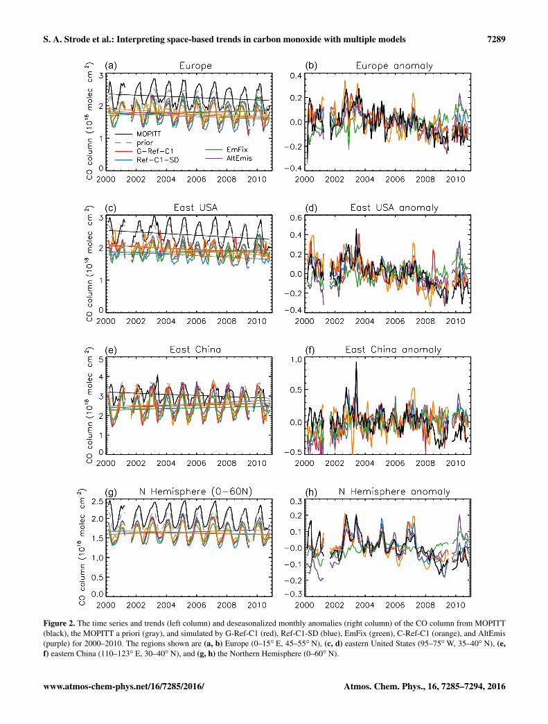
The hindcast simulations driven by MACCity emissions (G-Ref-C1, Ref-C1-SD, and C-Ref-C1) show negative trendsin CO over the US and Europe that agree with the ob-served slope from MOPITT within the uncertainty (Fig. 2,Table 2). The MOPITT trends for both regions are statisti-cally significant for both regions, as shown by Worden etal. (2013). These results are consistent with the findings of

www.atmos-chem-phys.net/16/7285/2016/ Atmos. Chem. Phys., 16, 7285–7294, 2016

7288 S. A. Strode et al.: Interpreting space-based trends in carbon monoxide with multiple models

Table 1. Description of simulations.

Simulation Model Meteorology Anthropogenic emissions Biomass burning emissions

G-Ref-C1 GEOSCCM internally derived MACCity MACCity, GFED3 (2009–2010)C-Ref-C1 CAM4-Chem internally derived MACCity MACCity, then repeat 2008Ref-C1-SD GMI MERRA MACCity same as GEOSCCMEmFix GMI MERRA fixed at 2000 fixed at 2000AltEmis GMI MERRA Strode et al. (2015b) GFED3

Table 2. Regional trends and correlations: (a) trendsa,b and (b) correlation coefficient (r) with monthly MOPITT anomaliesd,e.

(a) Years E. USA Europe E. China N. Hemisphere

G-Ref-C1c 2000-2010 −2.2 (0.38) −1.8 (0.42) 2.2 (1.1) −0.76 (3.0)C-Ref-C1c 2000–2010 −3.4 (0.54) −2.9 (0.50) 1.4 (1.4) −0.90 (3.0)Ref-C1-SDc 2000–2010 −2.4 (0.53) −1.6 (0.59) 1.4 (1.1) −0.76 (3.0)EmFixc 2000–2010 1.3 (0.55) 1.5 (0.44) 2.1 (0.87) 0.96 (2.5)AltEmisc 2000-2010 0.71 (0.73) 0.74 (0.66) 3.8 (1.4) 1.1 (3.4)MOPITT 2000–2010 −2.5 (0.64) −1.8 (0.69) −2.9 (1.8) −1.4 (2.8)MOPITT 2000–2014 −2.1 (0.41) −1.7 (0.43) −3.1 (1.1) −1.4 (1.7)

(b) Years E. USA Europe E. China N. Hemisphere

G-Ref-C1 2000–2010 0.26 0.39 0.061 0.71C-Ref-C1 2000–2010 0.23 0.36 0.18 0.62Ref-C1-SD 2000–2010 0.43 0.51 0.39 0.73EmFix 2000–2010 0.10 0.21 0.071 0.059AltEmis 2000–2010 0.55 0.59 0.48 0.69

a 1016 molec cm−2 yr−1, b 1σ uncertainty given in parentheses, c simulation results convolved with MOPITTaveraging kernel and a priori, d correlations are calculated from the detrended and deseasonalized time series.e Statistically significant correlations at the 95 % confidence level are indicated in bold.

Yin et al. (2015), whose inversion of MOPITT data showeda posteriori trends in CO emissions over the US and westernEurope that were consistent with but slightly larger than thea priori trends. The EmFix hindcast shows a positive, thoughnon-significant, trend for both regions, indicating that thedecrease in CO emissions is necessary for reproducing thedownward trend in the CO column. The AltEmis simulationfails to produce the negative trends, despite including nega-tive trends in regional emissions for both the US and Europe.The impact of these negative regional trends is insufficient toovercome the positive global emission trend in the AltEmisscenario (Fig. 1), leading to positive trends in CO.

Figure 2 also reveals a negative bias in the simulated COcolumn between the models and MOPITT. A low bias insimulated CO at northern latitudes is often present in globalmodels (Naik et al., 2013) and may indicate a high bias innorthern hemispheric OH (Strode et al., 2015a) or CO drydeposition (Stein et al., 2014), as well as an underestimate ofCO emissions.

The deseasonalized anomalies in the MOPITT and simu-lated CO columns are shown in Fig. 2b and d; the correlationcoefficients between the observed and simulated monthlyanomalies are presented in Table 2b. The highest correlationsare for the AltEmis and Ref-C1-SD simulations of the GMI

CTM. This result is consistent with the use of year-specificmeteorology, which we expect to better match the transportof particular years. The lowest correlations are for the EmFixsimulation. This is expected since the EmFix simulation doesnot include inter-annual variability (IAV) in biomass burning.The IAV in biomass burning makes a large contribution to theIAV of CO (Voulgarakis et al., 2015).

The role of biomass burning in driving the CO variabil-ity is even more evident at the hemispheric scale. Figure 2gand h show the anomalies in MOPITT and the simulationsfor the Northern Hemisphere (0–60◦ N). The EmFix simu-lation shows almost no correlation, while the other simula-tions have correlation coefficients exceeding 0.6 (Table 2).The role of changing anthropogenic emissions is also evi-dent, as the Ref-C1-SD simulation captures the 2008–2009dip in the CO column while the EmFix simulation does not.Gratz et al. (2015) found decreasing CO concentrations atMount Bachelor Observatory in Oregon during spring for2004–2013, which they attribute to reductions in emissionsleading to a lower hemispheric background. We also note thatRef-C1-SD and G-Ref-C1 have similar correlations with theobserved variability for the Northern Hemisphere (Table 2),indicating that transport differences are less important forvariability at the hemispheric scale.

Atmos. Chem. Phys., 16, 7285–7294, 2016 www.atmos-chem-phys.net/16/7285/2016/

S. A. Strode et al.: Interpreting space-based trends in carbon monoxide with multiple models 7289

Figure 2. The time series and trends (left column) and deseasonalized monthly anomalies (right column) of the CO column from MOPITT(black), the MOPITT a priori (gray), and simulated by G-Ref-C1 (red), Ref-C1-SD (blue), EmFix (green), C-Ref-C1 (orange), and AltEmis(purple) for 2000–2010. The regions shown are (a, b) Europe (0–15◦ E, 45–55◦ N), (c, d) eastern United States (95–75◦W, 35–40◦ N), (e,f) eastern China (110–123◦ E, 30–40◦ N), and (g, h) the Northern Hemisphere (0–60◦ N).

www.atmos-chem-phys.net/16/7285/2016/ Atmos. Chem. Phys., 16, 7285–7294, 2016

7290 S. A. Strode et al.: Interpreting space-based trends in carbon monoxide with multiple models

3.2 Trend over China

Observations from MOPITT show a negative trend in the COcolumn over eastern China for 2002–2012 (Worden et al.,2013). The negative trend for the years 2000–2014 exceedsthat for 2000–2010 (Table 2), showing that it is not drivensolely by temporary emission reductions in 2008. Our sim-ulations do not reproduce this trend, and instead show in-creases in the CO column (Fig. 2e), which is expected giventhat CO emissions from China increase in four of the fivesimulations. The anomalies (Fig. 2f) show that the discrep-ancy in the simulated versus observed trends is driven largelyby the failure of the simulations to capture the 2008 dip inthe CO column, leading to an overestimate that continuesthrough 2010. This suggests emission reductions in Chinaduring this time period are not adequately captured by theemission inventories. However, the good agreement betweenthe observed and simulated decreases in CO for the NorthernHemisphere as a whole (Fig. 2g, h) suggest that on a globalscale, the emission time series is reasonable. Consequently,we examine several other factors that may contribute to thedifference in sign between the MOPITT and simulated COtrends.

Regional trends in CO are expected to vary with altitude,with surface concentrations most heavily influenced by lo-cal emissions. MOPITT TIR retrievals have higher sensitiv-ity to CO in the mid-troposphere than at the surface (Deeteret al., 2004), so the trend in the MOPITT CO column will beweighted towards the trends in free tropospheric CO ratherthan near-surface CO. We quantify this impact on our Ref-C1-SD CO column trends by comparing the trend in thepure-model CO column with that of the simulated columnconvolved with the MOPITT averaging kernels.

The simulated CO trend over eastern China for 2000–2010 is positive (but not significant) both with and withoutthe averaging kernels, but application of the MOPITT ker-nels increases the positive trend from 1.3× 1016 to 1.4×1016 molec cm−2 yr−1. This result is initially surprising sincewe expect trends in the mid-troposphere to be more stronglyinfluenced by the decrease in the hemispheric CO back-ground. Indeed, the trends in CO concentration over easternChina simulated in Ref-C1-SD switch from positive in thelower troposphere to negative in the middle and upper tro-posphere. However, the application of the kernels results inmore positive (or less negative) trends in all regions.

Yoon et al. (2013) show that since the averaging kernelsvary over time, a bias between the true atmosphere and thea priori assumed by MOPITT can lead to an artificial trendin the retrieved CO. Similarly, the bias between the averagesimulated CO concentrations and the MOPITT a priori, ev-ident in Fig. 2, can lead to an artifact in the simulated COtrend when the simulation is convolved with the MOPITTaveraging kernels. This is due to the changing contributionof the a priori when the vertical sensitivity (averaging ker-nel) is varying in time. MOPITT vertical sensitivity varies

with time due to instrument degradation as well as the changein CO abundance. The bias in CO varies with altitude, soif the vertical sensitivity described by the averaging kernelchanges, this will change the value of the convolved CO col-umn even if there were no changes in the CO profile. Further-more, changes in the averaging kernel result in more or lessweight placed on the a priori versus the CO simulated by themodel. Thus, a difference between the a priori and the modelmeans that placing more (or less) weight on the a priori willchange the resulting value of Csim. Since the a priori profilesand columns are constant in time, taking the time derivativeof Eq. (1) yields

∂Csim/∂t = a(∂xmod/∂t)+ ∂a/∂t (xmod− x0). (3)

The second term on the right-hand side shows that thelarger the bias between the modeled CO and the a priori, thelarger the impact of the changing averaging kernel.

We quantify this effect by convolving the simulated COfor each year with the MOPITT averaging kernels for theyear 2008, thus removing the effect of the time depen-dence of the averaging kernels. The resulting trend, 0.56×1016 molec cm−2 yr−1, is less positive than the pure modeltrend or the original simulated trend. Thus, accounting forthe time dependence of the averaging kernels convolved withmodel bias reduces but does not eliminate the discrepancywith the observed trend. Comparing the trend for the con-stant averaging kernel case with the original simulated trendfor Ref-C1-SD (1.4× 1016 molec cm−2 yr−1) suggests thatthe changing averaging kernels combined with the modelbias contribute 0.84×1016 molec cm−2 yr−1 to the simulatedtrend. Other regions also show a more negative trend whenthe same averaging kernel is applied to the model results forall years. The large bias in CO at middle and high northernlatitudes commonly seen in modeling studies thus impactsthe ability of models to reproduce and attribute observedtrends in satellite data.

Figure 2 and Table 2 also show a positive trend in theGMI EmFix simulation for eastern China. This larger trendin the EmFix simulation than the Ref-C1-SD simulation in-dicates that the net decrease in emissions contributes to de-creasing CO over eastern China, consistent with the observednegative trend, but other factors in the model cause an in-crease in CO over eastern China even when all emissionsare constant. Subtracting the EmFix trend from the Ref-C1-SD trend shows that the changing emissions contribute aCO trend of −0.7 molec cm2 yr−1 over eastern China. The2.1 molec cm2 yr−1 trend in the EmFix simulation, which re-flects the impacts of the simulated chemistry and transport,thus contributes to the erroneous sign of the trend in theGMI simulations. The trends in the EmFix simulation for thenorthern hemispheric average and the eastern United Statesand Europe are positive as well (Table 2). We examine theircause in the next section.

Atmos. Chem. Phys., 16, 7285–7294, 2016 www.atmos-chem-phys.net/16/7285/2016/

S. A. Strode et al.: Interpreting space-based trends in carbon monoxide with multiple models 7291

(a) (b) (c)

Figure 3. Deseasonalized monthly anomalies in the total ozone column (left), mean tropospheric OH (center), and CO column (right) fromthe EmFix simulation as a function of latitude and month.

3.3 Contribution of OH interannual variability

Since the EmFix simulation shows a positive trend in theNorthern Hemisphere, we next examine the variability in theCO sink, OH. We also examine variability in the total ozonecolumn, since overhead ozone is a major driver of OH vari-ability (Duncan and Logan, 2008). Figure 3 shows the vari-ability in CO and OH in the EmFix simulation. The positiveand negative anomalies in CO correspond with the negativeand positive anomalies, respectively, in OH. The anomaliesin OH are in turn inversely related to anomalies in the to-tal ozone column. The correlation coefficient between OHand column ozone is −0.53 for the 15◦ S–15◦ N average,−0.72 for the 15–25◦ N average, and−0.75 for the 30–60◦ Naverage. The large NH ozone anomaly in 2010, in particu-lar, leads to a large anomaly in OH and thus CO. This OHanomaly extends from the northern tropics to the midlati-tudes. The large CO anomaly near the end of the time seriescontributes to the apparent 11-year trend. We note that sincethe lifetime of CO is several months, CO anomalies are notexpected to have a one-to-one correspondence with the OHanomalies.

The large anomaly in the simulated total ozone columnin 2010 is overestimated compared to observations. Figure 4shows the time dependence of the total ozone column from30 to 60◦ N in EmFix compared to SBUV data (Frith et al.,2014). While the observations show an anomaly in 2010, themagnitude is smaller than that produced by the simulation.Steinbrecht et al. (2011) attribute the 2010 anomaly in north-ern midlatitude ozone observations to a combination of anunusually strong negative Arctic Oscillation and North At-lantic Oscillation and the easterly phase of the quasi-biennialoscillation.

Figure 4. Monthly ozone column (a) and deseasonalized ozone col-umn anomaly (b) in SBUV data (black) and the EmFix simulation(green) for 30–60◦ N.

While the impact of OH interannual variability on the ap-parent trend in CO is clear in the EmFix simulation, thissource of variability is partially masked by large interannualvariability in CO emissions in the other simulations. We ex-amine the correlation between the detrended and deseasonal-ized CO anomalies from 10◦ S–10◦ N in the Ref-C1-SD sim-ulation and the CO emissions as well as the simulated OHand column ozone. Since the CO emitted in a given monthcan influence concentrations for several subsequent months,we use a 3-month smoothing of the emission time series. Wefind a high correlation (r = 0.88) between the CO anoma-lies and the CO emissions. This correlation is also evidentin the MOPITT data, as the MOPITT CO anomalies have acorrelation of r = 0.70 with the emissions. Figure 5 showsthe strong relationship between the simulated CO anomaliesand the CO emissions. However, the colors in Fig. 5 indicate

www.atmos-chem-phys.net/16/7285/2016/ Atmos. Chem. Phys., 16, 7285–7294, 2016

7292 S. A. Strode et al.: Interpreting space-based trends in carbon monoxide with multiple models

Figure 5. Monthly simulated CO column anomalies from the Ref-C1-SD simulation as a function of CO emissions for 10◦ S–10◦ N.Colors indicate the simulated OH column anomaly for the givenmonth.

that the scatter for a given level of emissions is often linkedto the OH anomalies, with low/high OH anomalies leadingto CO that is higher/lower than would be predicted just fromthe CO emissions. We find that the 10◦ S–10◦ N OH in theRef-C1-SD simulation is anticorrelated with CO (r =−0.62)and with the total ozone column (r =−0.68). Consequently,the simulated ozone column plays a role in modulating trop-ical CO variability even when variable CO emissions are in-cluded, although the emissions still play the strongest role.

4 Conclusions

We conducted a series of multi-year simulations to analyzethe causes of the negative trends in MOPITT CO reportedby Worden et al. (2013). Both CTM and CCM simulationsdriven by the MACCity emissions reproduce the observedtrends over the eastern United States and Europe, providingconfidence in the regional emission trends.

None of the simulations reproduce the observed nega-tive trend over eastern China. This negative trend persistseven with the MOPITT data extended out to 2014. TheMOPITT averaging kernels are weighted towards the freetroposphere, where the relative importance of hemisphericversus local trends is greater. However, our simulations in-dicate that this effect is insufficient to explain the nega-tive trends over China. Indeed, the negative trend in MO-PITT CO over eastern China (−2.9×1016 molec cm−2 yr−1)

is stronger than that of the northern hemispheric average(−1.4× 1016 molec cm−2 yr−1), indicating that changes inhemispheric CO account for less than half of the trendover China. While the simulations’ underestimate of the ob-served trend likely indicates a too positive emission trendfor China, several other factors play a role in the model–observation mismatch. We find that the time-dependent MO-PITT averaging kernels, combined with the low bias in sim-

ulated CO, provide a positive component to the simulatedtrends. Large anomalies in the simulated ozone column inthe GMI CTM simulations also contribute a positive com-ponent to the northern hemispheric trends due to their im-pact on OH. For the Ref-C1-SD simulation, the trends dueto the model bias combined with changing averaging kernels(0.84× 1016 molec cm−2 yr−1) and to the simulated chem-istry and transport (2.1×1016 molec cm−2 yr−1) can togetheraccount for almost 70 % of the 4.3× 1016 molec cm−2 yr−1

difference between the Ref-C1-SD and MOPITT trends overeastern China.

Variability in emissions is the primary driver of year-to-year variability in simulated CO, but OH variability alsoplays a role. The simulated OH is anti-correlated with bothCO and the total ozone column, highlighting the importanceof realistic overhead ozone columns for accurately simulat-ing CO variability and trends. In addition, further work isneeded to understand recent changes in CO emissions fromChina.

The Supplement related to this article is available onlineat doi:10.5194/acp-16-7285-2016-supplement.

Acknowledgements. This work was supported by NASA’s Mod-eling, Analysis, and Prediction Program and computing resourcesfrom the NASA High-End Computing Program. We thank BruceVan Aartsen for contributing to the GMI simulations. The CESMproject is supported by the National Science Foundation and theOffice of Science (BER) of the US Department of Energy. The MO-PITT project is supported by the NASA Earth Observing System(EOS) Program. The National Center for Atmospheric Research(NCAR) is sponsored by the National Science Foundation.

Edited by: A. Gettelman

References

Angelbratt, J., Mellqvist, J., Simpson, D., Jonson, J. E., Blumen-stock, T., Borsdorff, T., Duchatelet, P., Forster, F., Hase, F.,Mahieu, E., De Mazière, M., Notholt, J., Petersen, A. K., Raffal-ski, U., Servais, C., Sussmann, R., Warneke, T., and Vigouroux,C.: Carbon monoxide (CO) and ethane (C2H6) trends fromground-based solar FTIR measurements at six European stations,comparison and sensitivity analysis with the EMEP model, At-mos. Chem. Phys., 11, 9253–9269, doi:10.5194/acp-11-9253-2011, 2011.

Bey, I., Jacob, D., Logan, J., and Yantosca, R.: Asian chem-ical outflow to the Pacific in spring: Origins, pathways,and budgets, J. Geophys. Res.-Atmos., 106, 23097–23113,doi:10.1029/2001JD000806, 2001.

Crutzen, P.: A Discussion of the Chemistry of Some Minor Con-stituents in the Stratosphere and Troposphere, Pure Appl. Geo-phys., 106, 1385–1399, doi:10.1007/BF00881092, 1973.

Atmos. Chem. Phys., 16, 7285–7294, 2016 www.atmos-chem-phys.net/16/7285/2016/

S. A. Strode et al.: Interpreting space-based trends in carbon monoxide with multiple models 7293

Deeter, M., Emmons, L., Edwards, D., Gille, J., and Drummond,J.: Vertical resolution and information content of CO pro-files retrieved by MOPITT, Geophys. Res. Lett., 31, L15112,doi:10.1029/2004GL020235, 2004.

Deeter, M. N.: MOPITT (Measurements of Pollution in the Tro-posphere) Validated Version 4 Product User’s Guide, NationalCenter for Atmospheric Research, available at: http://web3.acd.ucar.edu/mopitt/v4_users_guide_val.pdf (last access: 27 Decem-ber 2013), 2009.

Deeter, M. N., Martinez-Alonso, S., Edwards, D. P., Emmons, L.K., Gille, J. C., Worden, H. M., Pittman, J. V., Daube, B. C.,and Wofsy, S. C.: Validation of MOPITT Version 5 thermal-infrared, near-infrared, and multispectral carbon monoxide pro-file retrievals for 2000–2011, J. Geophys. Res.-Atmos., 118,6710–6725, doi:10.1002/jgrd.50272, 2013.

Duncan, B. N. and Logan, J. A.: Model analysis of the factorsregulating the trends and variability of carbon monoxide be-tween 1988 and 1997, Atmos. Chem. Phys., 8, 7389–7403,doi:10.5194/acp-8-7389-2008, 2008.

Duncan, B. N., Strahan, S. E., Yoshida, Y., Steenrod, S. D., andLivesey, N.: Model study of the cross-tropopause transport ofbiomass burning pollution, Atmos. Chem. Phys., 7, 3713–3736,doi:10.5194/acp-7-3713-2007, 2007.

Edwards, D. P., Emmons, L. K., Hauglustaine, D. A., Chu, D.A., Gille, J. C., Kaufman, Y. J., Petron, G., Yurganov, L. N.,Giglio, L., Deeter, M. N., Yudin, V., Ziskin, D. C., Warner,J., Lamarque, J. F., Francis, G. L., Ho, S. P., Mao, D., Chen,J., Grechko, E. I., and Drummond, J. R.: Observations of car-bon monoxide and aerosols from the Terra satellite: NorthernHemisphere variability, J. Geophys. Res.-Atmos., 109, D24202,doi:10.1029/2004jd004727, 2004.

EPA: Our Nation’s Air – Status and Trends through 2010, edited by:EPA-454/R-12-001, Research Triangle Park, NC, 2011.

Eyring, V., Lamarque, J.-F., Hess, P., Arfeuille, F., Bowman, K.,Chipperfiel, M. P., Duncan, B., Fiore, A., Gettelman, A., andGiorgetta, M. A.: Overview of IGAC/SPARC Chemistry-ClimateModel Initiative (CCMI) community simulations in support ofupcoming ozone and climate assessments, Sparc Newsletter, 40,48–66, 2013.

Frith, S., Kramarova, N., Stolarski, R., McPeters, R., Bhartia, P., andLabow, G.: Recent changes in total column ozone based on theSBUV Version 8.6 Merged Ozone Data Set, J. Geophys. Res.-Atmos., 119, 9735–9751, 2014.

Granier, C., Bessagnet, B., Bond, T., D’Angiola, A., van der Gon,H. D., Frost, G. J., Heil, A., Kaiser, J. W., Kinne, S., Klimont,Z., Kloster, S., Lamarque, J. F., Liousse, C., Masui, T., Meleux,F., Mieville, A., Ohara, T., Raut, J. C., Riahi, K., Schultz, M.G., Smith, S. J., Thompson, A., van Aardenne, J., van der Werf,G. R., and van Vuuren, D. P.: Evolution of anthropogenic andbiomass burning emissions of air pollutants at global and re-gional scales during the 1980–2010 period, Climatic Change,109, 163–190, doi:10.1007/s10584-011-0154-1, 2011.

Gratz, L., Jaffe, D., and Hee, J.: Causes of increasing ozone anddecreasing carbon monoxide in springtime at the Mt. BachelorObservatory from 2004 to 2013, Atmos. Environ., 109, 323–330,doi:10.1016/j.atmosenv.2014.05.076, 2015.

uenther, A. B., Jiang, X., Heald, C. L., Sakulyanontvittaya, T., Duhl,T., Emmons, L. K., and Wang, X.: The Model of Emissions ofGases and Aerosols from Nature version 2.1 (MEGAN2.1): an

extended and updated framework for modeling biogenic emis-sions, Geosci. Model Dev., 5, 1471–1492, doi:10.5194/gmd-5-1471-2012, 2012.

He, H., Stehr, J. W., Hains, J. C., Krask, D. J., Doddridge, B.G., Vinnikov, K. Y., Canty, T. P., Hosley, K. M., Salawitch, R.J., Worden, H. M., and Dickerson, R. R.: Trends in emissionsand concentrations of air pollutants in the lower troposphere inthe Baltimore/Washington airshed from 1997 to 2011, Atmos.Chem. Phys., 13, 7859–7874, doi:10.5194/acp-13-7859-2013,2013.

Kurokawa, J., Ohara, T., Morikawa, T., Hanayama, S., Janssens-Maenhout, G., Fukui, T., Kawashima, K., and Akimoto, H.:Emissions of air pollutants and greenhouse gases over Asian re-gions during 2000–2008: Regional Emission inventory in ASia(REAS) version 2, Atmos. Chem. Phys., 13, 11019–11058,doi:10.5194/acp-13-11019-2013, 2013.

Lamarque, J.-F., Bond, T. C., Eyring, V., Granier, C., Heil, A.,Klimont, Z., Lee, D., Liousse, C., Mieville, A., Owen, B.,Schultz, M. G., Shindell, D., Smith, S. J., Stehfest, E., Van Aar-denne, J., Cooper, O. R., Kainuma, M., Mahowald, N., Mc-Connell, J. R., Naik, V., Riahi, K., and van Vuuren, D. P.: His-torical (1850–2000) gridded anthropogenic and biomass burningemissions of reactive gases and aerosols: methodology and ap-plication, Atmos. Chem. Phys., 10, 7017–7039, doi:10.5194/acp-10-7017-2010, 2010.

Li, L. and Liu, Y.: Space-borne and ground observations of the char-acteristics of CO pollution in Beijing, 2000–2010, Atmos. Envi-ron., 45, 2367–2372, doi:10.1016/j.atmosenv.2011.02.026, 2011.

Naik, V., Voulgarakis, A., Fiore, A. M., Horowitz, L. W., Lamar-que, J.-F., Lin, M., Prather, M. J., Young, P. J., Bergmann, D.,Cameron-Smith, P. J., Cionni, I., Collins, W. J., Dalsøren, S. B.,Doherty, R., Eyring, V., Faluvegi, G., Folberth, G. A., Josse, B.,Lee, Y. H., MacKenzie, I. A., Nagashima, T., van Noije, T. P. C.,Plummer, D. A., Righi, M., Rumbold, S. T., Skeie, R., Shindell,D. T., Stevenson, D. S., Strode, S., Sudo, K., Szopa, S., and Zeng,G.: Preindustrial to present-day changes in tropospheric hydroxylradical and methane lifetime from the Atmospheric Chemistryand Climate Model Intercomparison Project (ACCMIP), Atmos.Chem. Phys., 13, 5277–5298, doi:10.5194/acp-13-5277-2013,2013.

Ohara, T., Akimoto, H., Kurokawa, J., Horii, N., Yamaji, K., Yan,X., and Hayasaka, T.: An Asian emission inventory of an-thropogenic emission sources for the period 1980–2020, At-mos. Chem. Phys., 7, 4419–4444, doi:10.5194/acp-7-4419-2007,2007.

Oman, L. D., Ziemke, J. R., Douglass, A. R., Waugh, D. W., Lang,C., Rodriguez, J. M., and Nielsen, J. E.: The response of tropicaltropospheric ozone to ENSO, Geophys. Res. Lett., 38, L13706,doi:10.1029/2011gl047865, 2011.

Reynolds, R., Rayner, N., Smith, T., Stokes, D., and Wang,W.: An improved in situ and satellite SST analysis forclimate, J. Climate, 15, 1609–1625, doi:10.1175/1520-0442(2002)015<1609:AIISAS>2.0.CO;2, 2002.

Riahi, K., Grübler, A., and Nakicenovic, N.: Scenarios of long-termsocio-economic and environmental development under climatestabilization, Technol. Forecast. Soc., 74, 887–935, 2007.

Rienecker, M. M., Suarez, M. J., Gelaro, R., Todling, R., Bacmeis-ter, J., Liu, E., Bosilovich, M. G., Schubert, S. D., Takacs, L.,Kim, G.-K., Bloom, S., Chen, J., Collins, D., Conaty, A., da

www.atmos-chem-phys.net/16/7285/2016/ Atmos. Chem. Phys., 16, 7285–7294, 2016

7294 S. A. Strode et al.: Interpreting space-based trends in carbon monoxide with multiple models

Silva, A., Gu, W., Joiner, J., Koster, R. D., Lucchesi, R., Molod,A., Owens, T., Pawson, S., Pegion, P., Redder, C. R., Reichle,R., Robertson, F. R., Ruddick, A. G., Sienkiewicz, M., andWoollen, J.: MERRA: NASA’s Modern-Era Retrospective Anal-ysis for Research and Applications, J. Climate, 24, 3624–3648,doi:10.1175/JCLI-D-11-00015.1, 2011.

Stein, O., Schultz, M. G., Bouarar, I., Clark, H., Huijnen, V.,Gaudel, A., George, M., and Clerbaux, C.: On the wintertimelow bias of Northern Hemisphere carbon monoxide found inglobal model simulations, Atmos. Chem. Phys., 14, 9295–9316,doi:10.5194/acp-14-9295-2014, 2014.

Steinbrecht, W., Köhler, U., Claude, H., Weber, M., Burrows, J.P., and van der A, R. J.: Very high ozone columns at north-ern mid-latitudes in 2010, Geophys. Res. Lett., 38, L06803,doi:10.1029/2010GL046634, 2011.

Strahan, S. E., Duncan, B. N., and Hoor, P.: Observationally de-rived transport diagnostics for the lowermost stratosphere andtheir application to the GMI chemistry and transport model, At-mos. Chem. Phys., 7, 2435–2445, doi:10.5194/acp-7-2435-2007,2007.

Strode, S. A., Duncan, B. N., Yegorova, E. A., Kouatchou, J.,Ziemke, J. R., and Douglass, A. R.: Implications of carbonmonoxide bias for methane lifetime and atmospheric compo-sition in chemistry climate models, Atmos. Chem. Phys., 15,11789–11805, doi:10.5194/acp-15-11789-2015, 2015a.

Strode, S. A., Rodriguez, J. M., Logan, J. A., Cooper, O. R., Witte, J.C., Lamsal, L. N., Damon, M., Van Aartsen, B., Steenrod, S. D.,and Strahan, S. E.: Trends and variability in surface ozone overthe United States, J. Geophys. Res.-Atmos., 120, 9020–9042,2015b.

Thompson, A.: The Oxidizing Capacity of the Earth’s Atmosphere:Probable Past and Future Change, Science, 256, 1157–1165,doi:10.1126/science.256.5060.1157, 1992.

Tilmes, S., Lamarque, J.-F., Emmons, L. K., Kinnison, D. E.,Marsh, D., Garcia, R. R., Smith, A. K., Neely, R. R., Conley,A., Vitt, F., Val Martin, M., Tanimoto, H., Simpson, I., Blake,D. R., and Blake, N.: Representation of the Community EarthSystem Model (CESM1) CAM4-chem within the Chemistry-Climate Model Initiative (CCMI), Geosci. Model Dev., 9, 1853–1890, doi:10.5194/gmd-9-1853-2016, 2016.

Tohjima, Y., Kubo, M., Minejima, C., Mukai, H., Tanimoto, H.,Ganshin, A., Maksyutov, S., Katsumata, K., Machida, T., andKita, K.: Temporal changes in the emissions of CH4 and COfrom China estimated from CH4 / CO2 and CO / CO2 correla-tions observed at Hateruma Island, Atmos. Chem. Phys., 14,1663–1677, doi:10.5194/acp-14-1663-2014, 2014.

van der Werf, G. R., Randerson, J. T., Giglio, L., Collatz, G. J.,Kasibhatla, P. S., and Arellano Jr., A. F.: Interannual variabil-ity in global biomass burning emissions from 1997 to 2004, At-mos. Chem. Phys., 6, 3423–3441, doi:10.5194/acp-6-3423-2006,2006.

van der Werf, G. R., Randerson, J. T., Giglio, L., Collatz, G. J., Mu,M., Kasibhatla, P. S., Morton, D. C., DeFries, R. S., Jin, Y., andvan Leeuwen, T. T.: Global fire emissions and the contribution ofdeforestation, savanna, forest, agricultural, and peat fires (1997–2009), Atmos. Chem. Phys., 10, 11707-11735, doi:10.5194/acp-10-11707-2010, 2010.

van Donkelaar, A., Martin, R. V., Leaitch, W. R., Macdonald, A. M.,Walker, T. W., Streets, D. G., Zhang, Q., Dunlea, E. J., Jimenez,

J. L., Dibb, J. E., Huey, L. G., Weber, R., and Andreae, M. O.:Analysis of aircraft and satellite measurements from the Inter-continental Chemical Transport Experiment (INTEX-B) to quan-tify long-range transport of East Asian sulfur to Canada, At-mos. Chem. Phys., 8, 2999-3014, doi:10.5194/acp-8-2999-2008,2008.

Voulgarakis, A., Marlier, M., Faluvegi, G., Shindell, D., Tsi-garidis, K., and Mangeon, S.: Interannual variability of tropo-spheric trace gases and aerosols: The role of biomass burn-ing emissions, J. Geophys. Res.-Atmos., 120, 7157–7173,doi:10.1002/2014JD022926, 2015.

Wang, Y., Munger, J. W., Xu, S., McElroy, M. B., Hao, J., Nielsen,C. P., and Ma, H.: CO2 and its correlation with CO at a rural sitenear Beijing: implications for combustion efficiency in China,Atmos. Chem. Phys., 10, 8881–8897, doi:10.5194/acp-10-8881-2010, 2010.

Warner, J., Carminati, F., Wei, Z., Lahoz, W., and Attié, J.-L.: Tro-pospheric carbon monoxide variability from AIRS under clearand cloudy conditions, Atmos. Chem. Phys., 13, 12469–12479,doi:10.5194/acp-13-12469-2013, 2013.

Worden, H. M., Cheng, Y., Pfister, G., Carmichael, G. R., Zhang,Q., Streets, D. G., Deeter, M., Edwards, D. P., Gille, J.C., and Worden, J. R.: Satellite-based estimates of reducedCO and CO2 emissions due to traffic restrictions during the2008 Beijing Olympics, Geophys. Res. Lett., 39, L14802,doi:10.1029/2012GL052395, 2012.

Worden, H. M., Deeter, M. N., Frankenberg, C., George, M., Nichi-tiu, F., Worden, J., Aben, I., Bowman, K. W., Clerbaux, C., Co-heur, P. F., de Laat, A. T. J., Detweiler, R., Drummond, J. R.,Edwards, D. P., Gille, J. C., Hurtmans, D., Luo, M., Martínez-Alonso, S., Massie, S., Pfister, G., and Warner, J. X.: Decadalrecord of satellite carbon monoxide observations, Atmos. Chem.Phys., 13, 837–850, doi:10.5194/acp-13-837-2013, 2013.

Yin, Y., Chevallier, F., Ciais, P., Broquet, G., Fortems-Cheiney, A.,Pison, I., and Saunois, M.: Decadal trends in global CO emis-sions as seen by MOPITT, Atmos. Chem. Phys., 15, 13433–13451, doi:10.5194/acp-15-13433-2015, 2015.

Yoon, J. and Pozzer, A.: Model-simulated trend of surface carbonmonoxide for the 2001–2010 decade, Atmos. Chem. Phys., 14,10465–10482, doi:10.5194/acp-14-10465-2014, 2014.

Yoon, J., Pozzer, A., Hoor, P., Chang, D. Y., Beirle, S., Wagner,T., Schloegl, S., Lelieveld, J., and Worden, H. M.: TechnicalNote: Temporal change in averaging kernels as a source of uncer-tainty in trend estimates of carbon monoxide retrieved from MO-PITT, Atmos. Chem. Phys., 13, 11307–11316, doi:10.5194/acp-13-11307-2013, 2013.

Yumimoto, K., Uno, I., and Itahashi, S.: Long-term inverse model-ing of Chinese CO emission from satellite observations, Environ.Pollut., 195, 308–318, doi:10.1016/j.envpol.2014.07.026, 2014.

Zhang, Q., Streets, D. G., Carmichael, G. R., He, K. B., Huo, H.,Kannari, A., Klimont, Z., Park, I. S., Reddy, S., Fu, J. S., Chen,D., Duan, L., Lei, Y., Wang, L. T., and Yao, Z. L.: Asian emis-sions in 2006 for the NASA INTEX-B mission, Atmos. Chem.Phys., 9, 5131–5153, doi:10.5194/acp-9-5131-2009, 2009.

Zhao, Y., Nielsen, C. P., McElroy, M. B., Zhang, L., and Zhang,J.: CO emissions in China: Uncertainties and implications of im-proved energy efficiency and emission control, Atmos. Environ.,49, 103–113, doi:10.1016/j.atmosenv.2011.12.015, 2012.

Atmos. Chem. Phys., 16, 7285–7294, 2016 www.atmos-chem-phys.net/16/7285/2016/