Embed Size (px)
Citation preview
1
Interpreting Geology of Ashley Schiff Park Preserve
with New High-Resolution
Digital Elevation Model
By Tenzin Lhundup Stony Brook University
MPI Summer Scholars Program 2005 Stony Brook University
Faculty Advisors: Gilbert Hanson and Glenn Richard

2
Abstract
The objective of this study was to interpret the geomorphic features developed by
glaciers at Ashley Schiff Park Preserve and to study whether south part of Ashley Schiff
Park Preserve is Hummocky terrain or whether it is just a continuation of folding and
faulting process. This required creating a new high-resolution digital elevation model
(DEM) based on 2-foot contour interval with 1-meter grid cell size by using GIS software
ArcGIS v9.0 with its 3D Analyst extension. Ground Penetrating Radar (GPR) radargram
of 100MHz was also used to examine the subsurface structural trends and patterns.
Glacial features in north part of Preserve are developed from proglacial thrusting whereas
it is evident from new digital elevation model and GPR radargram that the southern part
of the preserve is more likely a hummocky terrain.
3
Introduction
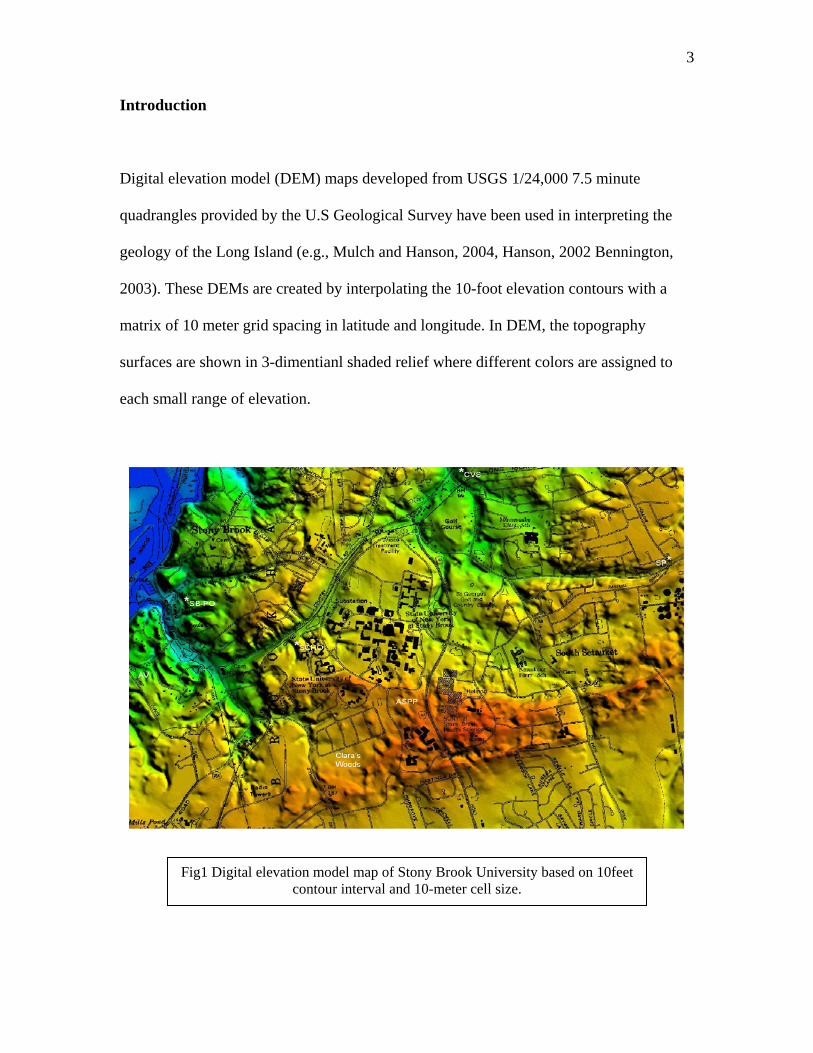
Digital elevation model (DEM) maps developed from USGS 1/24,000 7.5 minute
quadrangles provided by the U.S Geological Survey have been used in interpreting the
geology of the Long Island (e.g., Mulch and Hanson, 2004, Hanson, 2002 Bennington,
2003). These DEMs are created by interpolating the 10-foot elevation contours with a
matrix of 10 meter grid spacing in latitude and longitude. In DEM, the topography
surfaces are shown in 3-dimentianl shaded relief where different colors are assigned to
each small range of elevation.
Fig1 Digital elevation model map of Stony Brook University based on 10feet
contour interval and 10-meter cell size.
4
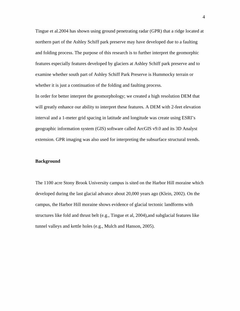
Tingue et al.2004 has shown using ground penetrating radar (GPR) that a ridge located at
northern part of the Ashley Schiff park preserve may have developed due to a faulting
and folding process. The purpose of this research is to further interpret the geomorphic
features especially features developed by glaciers at Ashley Schiff park preserve and to
examine whether south part of Ashley Schiff Park Preserve is Hummocky terrain or
whether it is just a continuation of the folding and faulting process.
In order for better interpret the geomorphology; we created a high resolution DEM that
will greatly enhance our ability to interpret these features. A DEM with 2-feet elevation
interval and a 1-meter grid spacing in latitude and longitude was create using ESRI’s
geographic information system (GIS) software called ArcGIS v9.0 and its 3D Analyst
extension. GPR imaging was also used for interpreting the subsurface structural trends.
Background
The 1100 acre Stony Brook University campus is sited on the Harbor Hill moraine which
developed during the last glacial advance about 20,000 years ago (Klein, 2002). On the
campus, the Harbor Hill moraine shows evidence of glacial tectonic landforms with
structures like fold and thrust belt (e.g., Tingue et al, 2004),and subglacial features like
tunnel valleys and kettle holes (e.g., Mulch and Hanson, 2005).
5
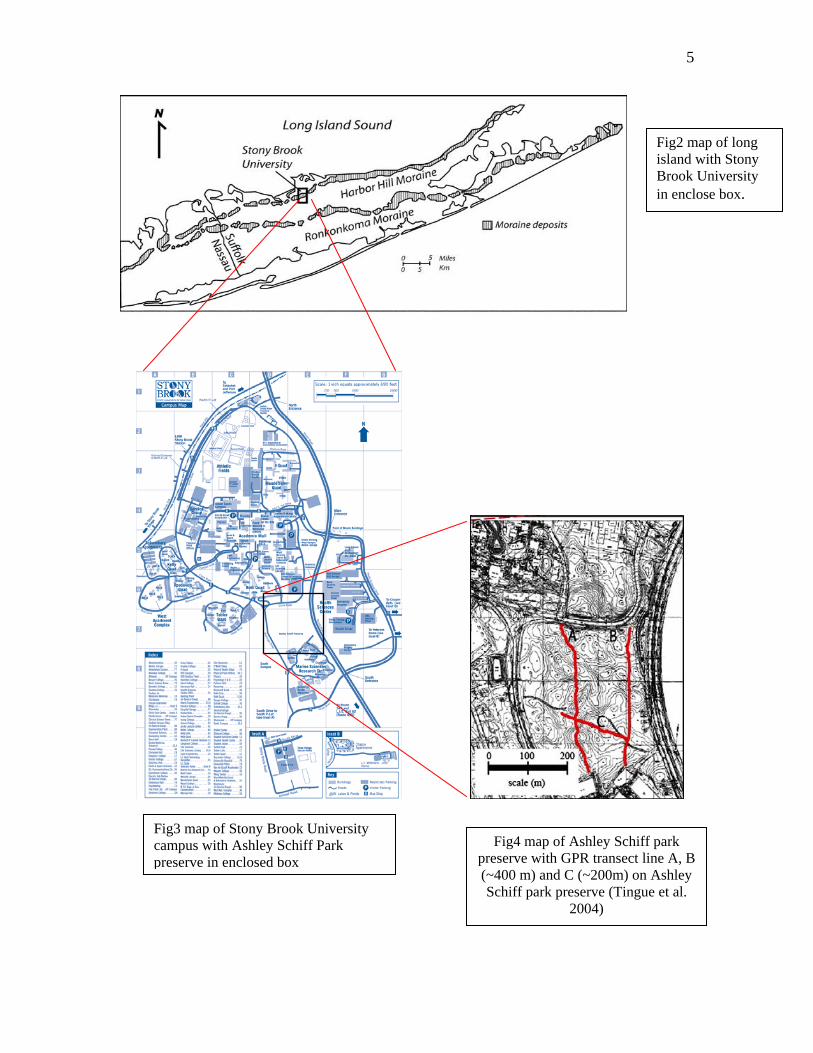
Fig2 map of long island with Stony Brook University in enclose box.
Fig3 map of Stony Brook University campus with Ashley Schiff Park preserve in enclosed box
Fig4 map of Ashley Schiff park
preserve with GPR transect line A, B (~400 m) and C (~200m) on Ashley Schiff park preserve (Tingue et al.
2004)
6
The Ashley Schiff park preserve with its 26.68 acres on the Stony Brook University
campus provides significant information about both the ecological and geological history
of Long Island and Stony Brook campus. Even after 20,000 years, the glacial geomorphic
features in the Ashley Schiff park preserve are still preserved due its erosion resistant
one-meter thick till layers coating the area. Till is an unsorted and unstratified mixture of
sediments like clay, silt, sand, gravel, cobble and boulders deposited directly from the
glacier. Ridges and valleys are dominant features in Ashley Schiff park preserve.
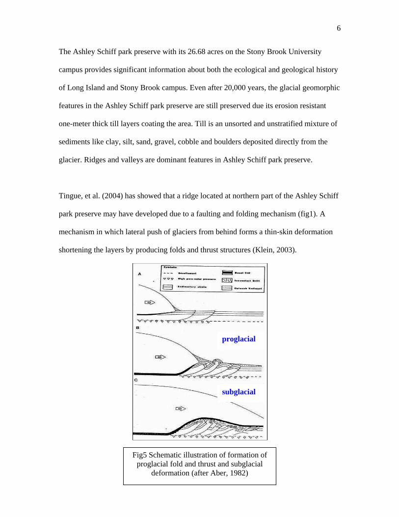
Tingue, et al. (2004) has showed that a ridge located at northern part of the Ashley Schiff
park preserve may have developed due to a faulting and folding mechanism (fig1). A
mechanism in which lateral push of glaciers from behind forms a thin-skin deformation
shortening the layers by producing folds and thrust structures (Klein, 2003).
proglacial
subglacial
Fig5 Schematic illustration of formation of proglacial fold and thrust and subglacial
deformation (after Aber, 1982)
7
However, there are other glacial features in Ashley Schiff park preserve especially in
south whose morphology has not been discussed yet. We believe that these features may
have developed from sediments deposited from subglacial and supraglacial deposits
forming a hummocky moraine.
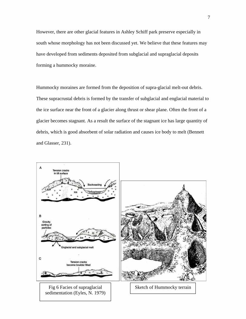
Hummocky moraines are formed from the deposition of supra-glacial melt-out debris.
These supracrustal debris is formed by the transfer of subglacial and englacial material to
the ice surface near the front of a glacier along thrust or shear plane. Often the front of a
glacier becomes stagnant. As a result the surface of the stagnant ice has large quantity of
debris, which is good absorbent of solar radiation and causes ice body to melt (Bennett
and Glasser, 231).
Fig 6 Facies of supraglacial
sedimentation (Eyles, N. 1979) Sketch of Hummocky terrain
8
Hummocky moraines are irregular and chaotic in appearance with many small hills
(approximately same elevation) and depressions with steep to gentle slopes without lack
of any consistent trend. (John Menzies, 332). It is as an irregular collection of mounds
and enclosed hollows often called knob and kettle terrain. (Bennett and Glasser, 231)
Method
A) Creating digital elevation model
See Appendix 1 for creating digital elevation model from contour line, break line and
property line together.
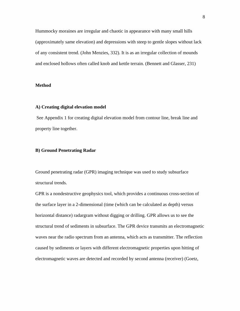
B) Ground Penetrating Radar
Ground penetrating radar (GPR) imaging technique was used to study subsurface
structural trends.
GPR is a nondestructive geophysics tool, which provides a continuous cross-section of
the surface layer in a 2-dimensional (time (which can be calculated as depth) versus
horizontal distance) radargram without digging or drilling. GPR allows us to see the
structural trend of sediments in subsurface. The GPR device transmits an electromagnetic
waves near the radio spectrum from an antenna, which acts as transmitter. The reflection
caused by sediments or layers with different electromagnetic properties upon hitting of
electromagnetic waves are detected and recorded by second antenna (receiver) (Goetz,
9
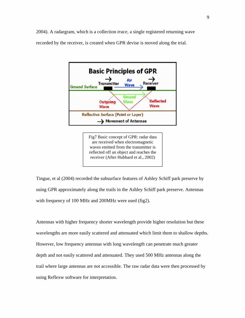
2004). A radargram, which is a collection trace, a single registered returning wave
recorded by the receiver, is created when GPR devise is moved along the trial.
Fig7 Basic concept of GPR: radar data are received when electromagnetic
waves emitted from the transmitter is reflected off an object and reaches the receiver (After Hubbard et al., 2002)
Tingue, et al (2004) recorded the subsurface features of Ashley Schiff park preserve by
using GPR approximately along the trails in the Ashley Schiff park preserve. Antennas
with frequency of 100 MHz and 200MHz were used (fig2).
Antennas with higher frequency shorter wavelength provide higher resolution but these
wavelengths are more easily scattered and attenuated which limit them to shallow depths.
However, low frequency antennas with long wavelength can penetrate much greater
depth and not easily scattered and attenuated. They used 500 MHz antennas along the
trail where large antennas are not accessible. The raw radar data were then processed by
using Reflexw software for interpretation.
10
Discussion
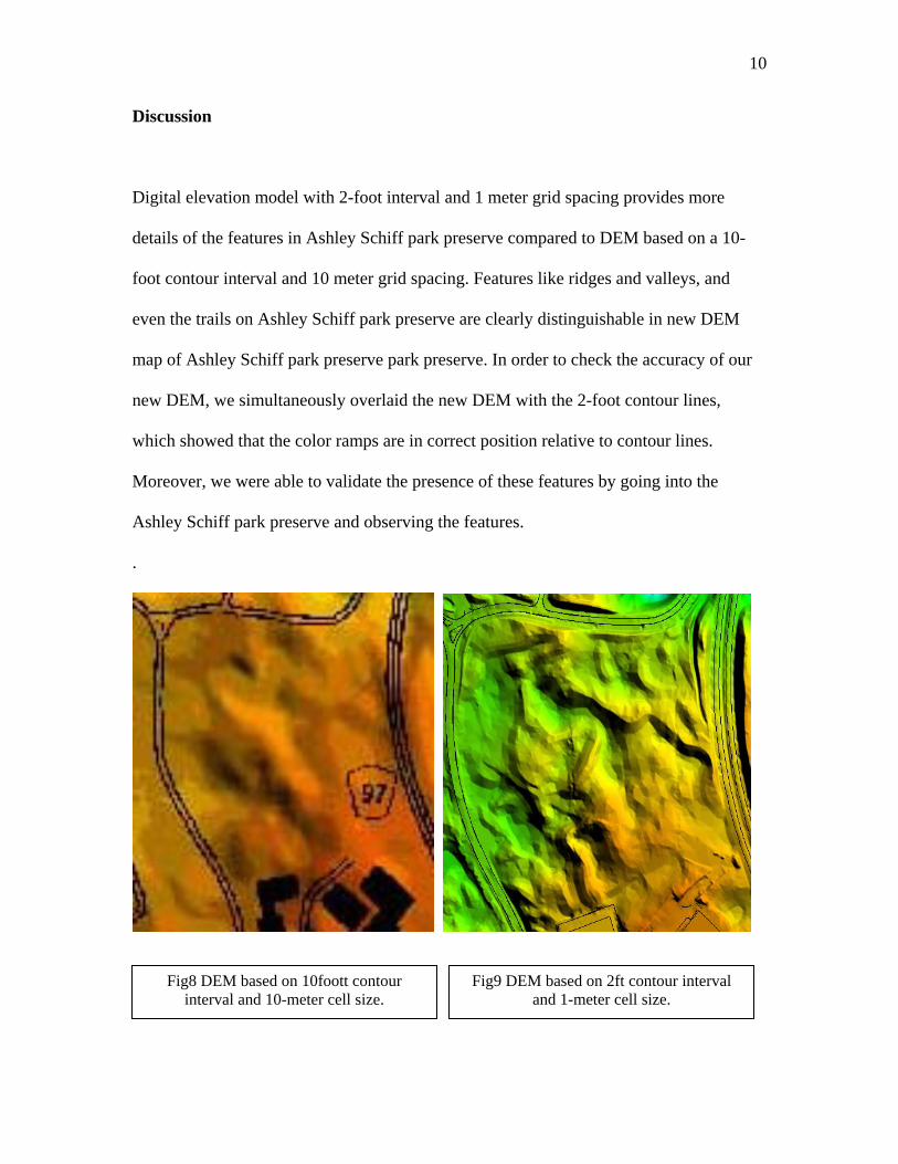
Digital elevation model with 2-foot interval and 1 meter grid spacing provides more
details of the features in Ashley Schiff park preserve compared to DEM based on a 10-
foot contour interval and 10 meter grid spacing. Features like ridges and valleys, and
even the trails on Ashley Schiff park preserve are clearly distinguishable in new DEM
map of Ashley Schiff park preserve park preserve. In order to check the accuracy of our
new DEM, we simultaneously overlaid the new DEM with the 2-foot contour lines,
which showed that the color ramps are in correct position relative to contour lines.
Moreover, we were able to validate the presence of these features by going into the
Ashley Schiff park preserve and observing the features.
.
Fig8 DEM based on 10foott contour
interval and 10-meter cell size. Fig9 DEM based on 2ft contour interval
and 1-meter cell size.
11
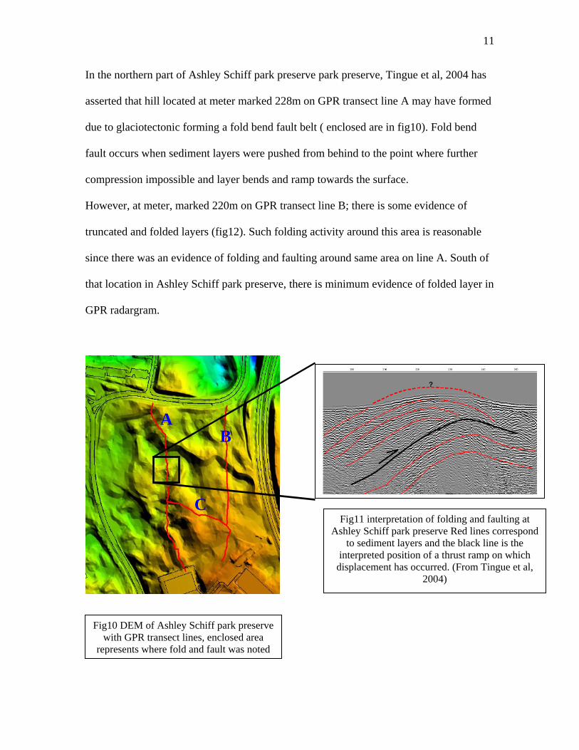
In the northern part of Ashley Schiff park preserve park preserve, Tingue et al, 2004 has
asserted that hill located at meter marked 228m on GPR transect line A may have formed
due to glaciotectonic forming a fold bend fault belt ( enclosed are in fig10). Fold bend
fault occurs when sediment layers were pushed from behind to the point where further
compression impossible and layer bends and ramp towards the surface.
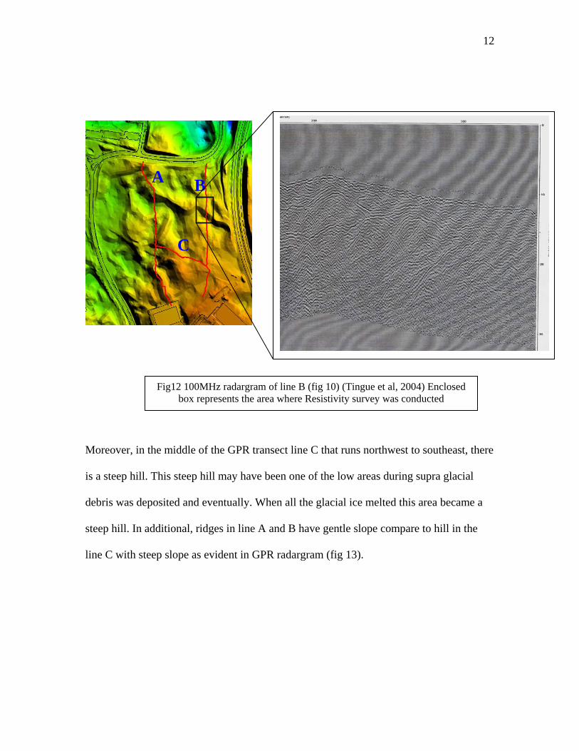
However, at meter, marked 220m on GPR transect line B; there is some evidence of
truncated and folded layers (fig12). Such folding activity around this area is reasonable
since there was an evidence of folding and faulting around same area on line A. South of
that location in Ashley Schiff park preserve, there is minimum evidence of folded layer in
GPR radargram.
Fig11 interpretation of folding and faulting at Ashley Schiff park preserve Red lines correspond
to sediment layers and the black line is the interpreted position of a thrust ramp on which
displacement has occurred. (From Tingue et al, 2004)
C
B A
Fig10 DEM of Ashley Schiff park preserve with GPR transect lines, enclosed area
represents where fold and fault was noted
12
A B
C
Fig12 100MHz radargram of line B (fig 10) (Tingue et al, 2004) Enclosed
box represents the area where Resistivity survey was conducted
Moreover, in the middle of the GPR transect line C that runs northwest to southeast, there
is a steep hill. This steep hill may have been one of the low areas during supra glacial
debris was deposited and eventually. When all the glacial ice melted this area became a
steep hill. In additional, ridges in line A and B have gentle slope compare to hill in the
line C with steep slope as evident in GPR radargram (fig 13).
13
A B
C
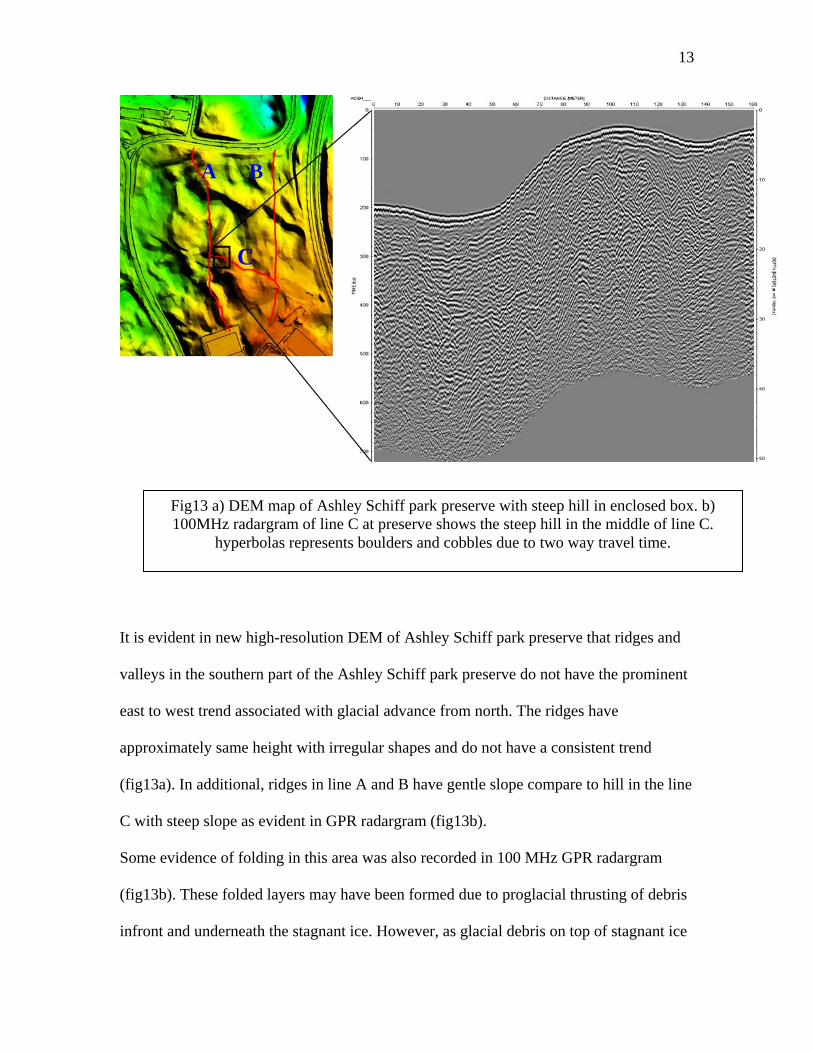
Fig13 a) DEM map of Ashley Schiff park preserve with steep hill in enclosed box. b) 100MHz radargram of line C at preserve shows the steep hill in the middle of line C.
hyperbolas represents boulders and cobbles due to two way travel time.
It is evident in new high-resolution DEM of Ashley Schiff park preserve that ridges and
valleys in the southern part of the Ashley Schiff park preserve do not have the prominent
east to west trend associated with glacial advance from north. The ridges have
approximately same height with irregular shapes and do not have a consistent trend
(fig13a). In additional, ridges in line A and B have gentle slope compare to hill in the line
C with steep slope as evident in GPR radargram (fig13b).
Some evidence of folding in this area was also recorded in 100 MHz GPR radargram
(fig13b). These folded layers may have been formed due to proglacial thrusting of debris
infront and underneath the stagnant ice. However, as glacial debris on top of stagnant ice
14
starts to absorb solar radiation and causes ice body to melt, these debris may have
backwashed or deposited which eventually resulted in this steep hill when all the ice body
was melted.
Conclusion
In conclusion, the purpose of our research is to interpret the geomorphic features on
Ashley Schiff Park Preserve and to investigate whether south part of Ashley Schiff Park
Preserve is Hummocky terrain or whether it is just a continuation of the folding and
faulting process. Through out new high-resolution digital elevation model map based on
2-foot contour interval with 1-meter grid cell size and with radargram data from GPR, the
southern part of the Ashley Schiff Park Preserve is most likely a hummocky terrain
because ridges and valley in south part of Ashley Schiff Park Preserve are irregular and
do not have consistent trend. In southern part of Preserve, there are hills with gentle slope
and others with steep slope however, most of them with approximately similar elevation
with irregular shaped kettle holes. However, glacial features in northern part of Ashley
Schiff Park Preserve have shown strong influence of proglacial thrusting and folding.
15
References Cited Aber, J.S., Model for glaciotectonism, Geological Society of Denmark, Bulletin, 39, 79-90, 1982. Bennett, Matthew R., and Glasser, Neil F, Glacial Geology: Ice Sheets and Landforms. England: John Wiley & Sons, 1996 Bennington, J B, “New Observations on the glacial geomorphology of Long Island from a Digital Elevation Model (DEM).” Program for the Eleventh Conference on "Geology of Long Island and Metropolitan New York" April 12, 2003 Department of Geology, Hofstra University, Hempstead, NY
http://pbisotopes.ess.sunysb.edu/lig/Conferences/abstracts 03/bennington/index.html
Eyles, N., Facies of supraglacial sedimentation on Icelandic and Alpine temperate glacier. Canadian Journal of Earth Science 16, 1341-1361
Farrell, Rob. “GIS Cookbook: Recipe - Define Projection for a Shapefile or Geodatabase.” CSISS. 26 Feb. 05 <http://www.csiss.org/cookbook/recipe/23> Goetz, Kurt T, and Dan M. Davis, Glacial tectonics at Hither Hills, eastern Long Island:
evidence from Ground Penetrating Radar. 2004 Dept. of Geosciences, SUNY Stony Brook http://pbisotopes.ess.sunysb.edu/lig/Conferences/abstracts-04/goetz.pdf
Hambrey, M. J., Glacial Environments. UCL Press: London, 1994. Hanson, Gilbert N., “Evaluation of Geomorphology of the Stony Brook-Setauket-Port Jefferson Area Based on Digital Elevation Models.” March 1, 2002 Dept. of Geosciences, SUNY Stony Brook, Stony Brook, NY http://pbisotopes.ess.sunysb.edu/reports/dem_2/
Klein, Charles E., “Glaciotectonic Shear Zones: Surface Sample Bias and Clast Fabric
Interpretation.” May, 2002 Dept. of Geosciences, SUNY Stony Brook, Stony Brook, NY http://pbisotopes.ess.sunysb.edu/reports/
Menzies, John, ed, Modern and Past Glacial Environment. Oxford: Butterworth-Heinemann, 2002 Mulch, Danielle., and Gilbert N. Hanson, “Port Jefferson Geomorphology.” 2005, Department of Geosciences, SUNY Stony Brook, Stony Brook, NY
http://pbisotopes.ess.sunysb.edu/lig/Conferences/abstracts05/abstracts/mulch-web/Port%20Jefferson.htm
Phil Hurvitz, http://gis.washington.edu/cfr250/lessons/data_export/#conv_feat_theme Tingue, Christopher., Dan M. Davis, and James D. Girardi “Anatomy of Glacio-tectonic Folding and Thrusting Imaged Using GPR in the Ashley Schiff Preserve” Program for the Eleventh Conference on "Geology of Long Island and Metropolitan New York" April 17, 2004 Dept. of Geosciences, SUNY Stony Brook, Stony Brook, NY

16
http://pbisotopes.ess.sunysb.edu/lig/Conferences/abstracts-04/tingue.pdf “Tutorial: Reprojecting Data with ArcGIS.” The University of Michigan. 2004. University Library. 22 Jul. 2004 <http://www.lib.umich.edu/nsds/tutspat/proj/arcgisproj.html> “Harvard Design School.” < http://www.gsd.harvard.edu/geo/manual/dem/> US GeoData Digital Elevation Models, Fact Sheet 040-00, USGS, April 2000 http://erg.usgs.gov/isb/pubs/factsheets/fs04000.html#dem
17
Appendix 1: Method for Creating Digital elevation model map
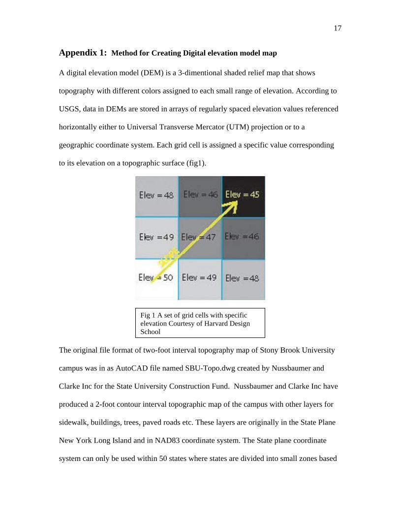
A digital elevation model (DEM) is a 3-dimentional shaded relief map that shows
topography with different colors assigned to each small range of elevation. According to
USGS, data in DEMs are stored in arrays of regularly spaced elevation values referenced
horizontally either to Universal Transverse Mercator (UTM) projection or to a
geographic coordinate system. Each grid cell is assigned a specific value corresponding
to its elevation on a topographic surface (fig1).
Fig 1 A set of grid cells with specific elevation Courtesy of Harvard Design School
The original file format of two-foot interval topography map of Stony Brook University
campus was in as AutoCAD file named SBU-Topo.dwg created by Nussbaumer and
Clarke Inc for the State University Construction Fund. Nussbaumer and Clarke Inc have
produced a 2-foot contour interval topographic map of the campus with other layers for
sidewalk, buildings, trees, paved roads etc. These layers are originally in the State Plane
New York Long Island and in NAD83 coordinate system. The State plane coordinate
system can only be used within 50 states where states are divided into small zones based
18
on political boundary. On the other hand, in UTM coordinate system, earth is divided into
sixty 6-degree-wide zones between 84 degrees N and 80 degrees S. North American
Datum (NAD) 1927 or 1983 is used mostly for areas in North America. As a reference
system, this based on the size and shape of the earth.
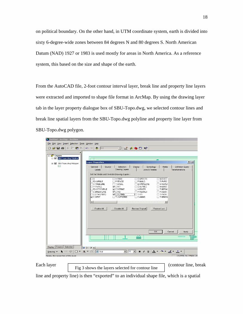
From the AutoCAD file, 2-foot contour interval layer, break line and property line layers
were extracted and imported to shape file format in ArcMap. By using the drawing layer
tab in the layer property dialogue box of SBU-Topo.dwg, we selected contour lines and
break line spatial layers from the SBU-Topo.dwg polyline and property line layer from
SBU-Topo.dwg polygon.
Each layer (contour line, break
line and property line) is then “exported” to an individual shape file, which is a spatial
Fig 3 shows the layers selected for contour line
19
data format of ArcGIS. Detail instruction on exporting the data into shape file is provided
by Hurvitz at http://gis.washington.edu/cfr250/lessons/data_export/#conv_feat_theme
In order to overlay one or more layer from same or different source in ArcMap
simultaneously, it is important to have all the data with similar coordinate system. For
instance, a layer with state plane coordinate system cannot be overlaid with layer with
UTM coordinate system. However, one can reproject the layer with state plane into UTM
coordinate system since UTM is in metric system (in meter) and state plane is in US
metric system (in feet).
Reprojecting the Layers
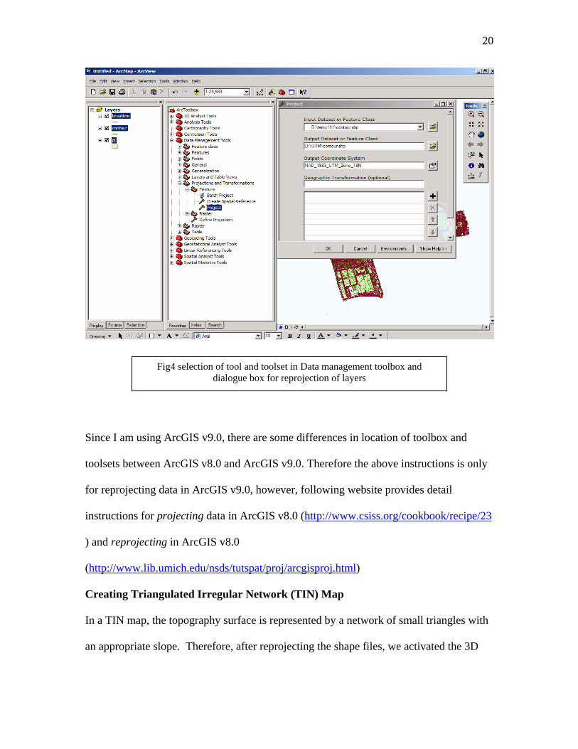
The coordinate system of the contour lines, break lines and property line is in state plane
New York Long Island and in North American Datum 1983 are reprojected in to UTM
zone 18N with North American Datum 1983, by using the “Project” tool under the
projection and transformation toolset in the Data management toolbox.
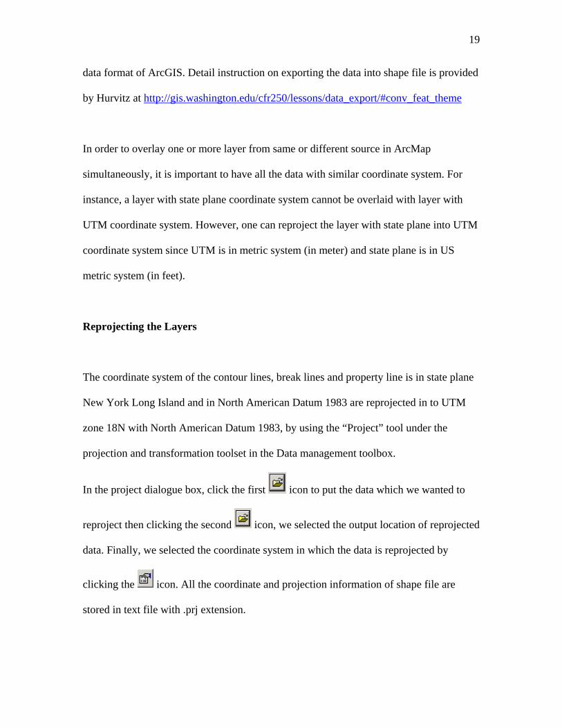
In the project dialogue box, click the first icon to put the data which we wanted to
reproject then clicking the second icon, we selected the output location of reprojected
data. Finally, we selected the coordinate system in which the data is reprojected by
clicking the icon. All the coordinate and projection information of shape file are
stored in text file with .prj extension.
20
Fig4 selection of tool and toolset in Data management toolbox and
dialogue box for reprojection of layers
Since I am using ArcGIS v9.0, there are some differences in location of toolbox and
toolsets between ArcGIS v8.0 and ArcGIS v9.0. Therefore the above instructions is only
for reprojecting data in ArcGIS v9.0, however, following website provides detail
instructions for projecting data in ArcGIS v8.0 (http://www.csiss.org/cookbook/recipe/23
) and reprojecting in ArcGIS v8.0
(http://www.lib.umich.edu/nsds/tutspat/proj/arcgisproj.html)
Creating Triangulated Irregular Network (TIN) Map
In a TIN map, the topography surface is represented by a network of small triangles with
an appropriate slope. Therefore, after reprojecting the shape files, we activated the 3D
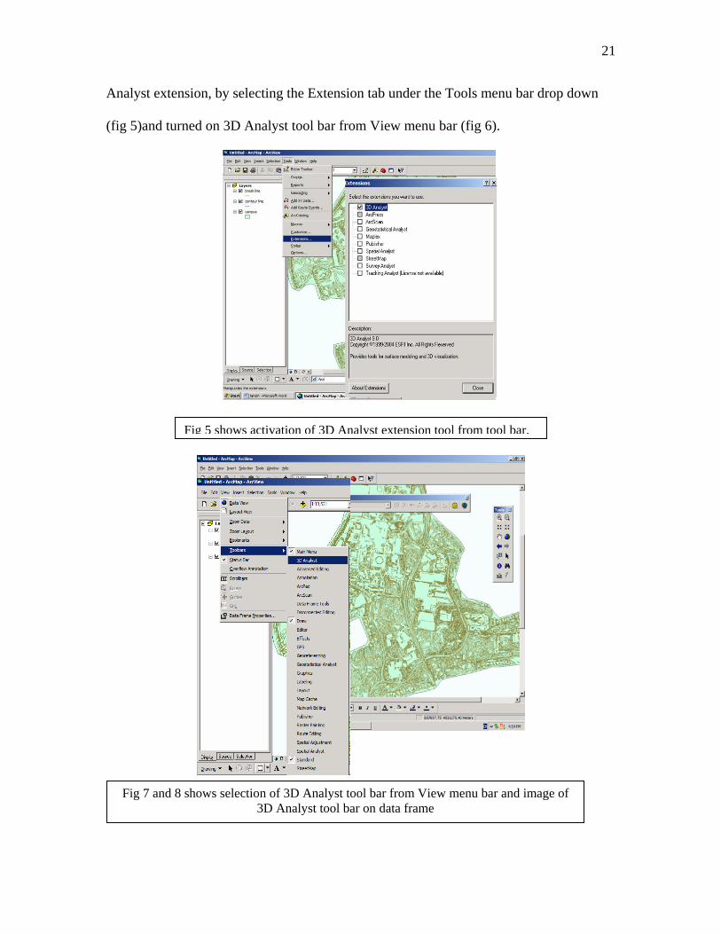
21
Analyst extension, by selecting the Extension tab under the Tools menu bar drop down
(fig 5)and turned on 3D Analyst tool bar from View menu bar (fig 6).
Fig 5 shows activation of 3D Analyst extension tool from tool bar.
Fig 7 and 8 shows selection of 3D Analyst tool bar from View menu bar and image of 3D Analyst tool bar on data frame
22
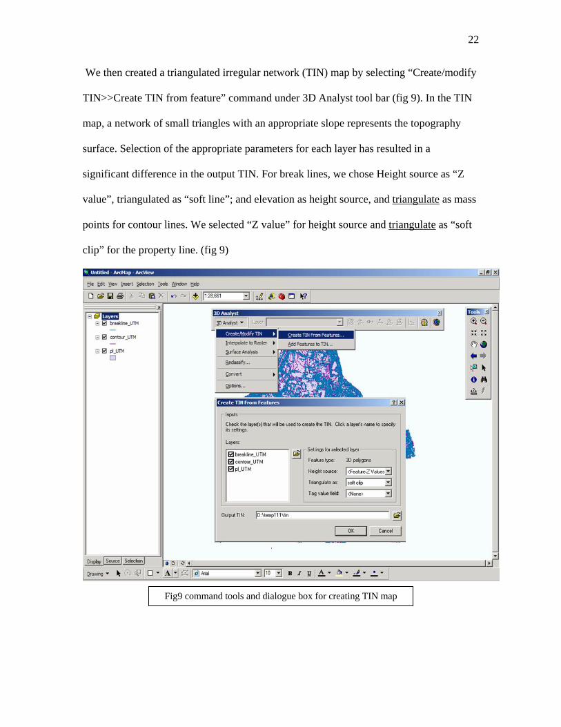
We then created a triangulated irregular network (TIN) map by selecting “Create/modify
TIN>>Create TIN from feature” command under 3D Analyst tool bar (fig 9). In the TIN
map, a network of small triangles with an appropriate slope represents the topography
surface. Selection of the appropriate parameters for each layer has resulted in a
significant difference in the output TIN. For break lines, we chose Height source as “Z
value”, triangulated as “soft line”; and elevation as height source, and triangulate as mass
points for contour lines. We selected “Z value” for height source and triangulate as “soft
clip” for the property line. (fig 9)
Fig9 command tools and dialogue box for creating TIN map
23
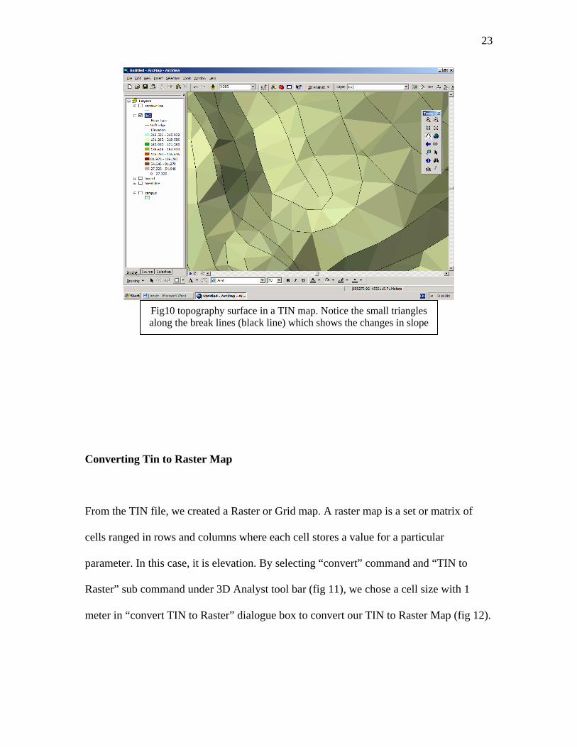
Fig10 topography surface in a TIN map. Notice the small triangles along the break lines (black line) which shows the changes in slope
Converting Tin to Raster Map
From the TIN file, we created a Raster or Grid map. A raster map is a set or matrix of
cells ranged in rows and columns where each cell stores a value for a particular
parameter. In this case, it is elevation. By selecting “convert” command and “TIN to
Raster” sub command under 3D Analyst tool bar (fig 11), we chose a cell size with 1
meter in “convert TIN to Raster” dialogue box to convert our TIN to Raster Map (fig 12).
24
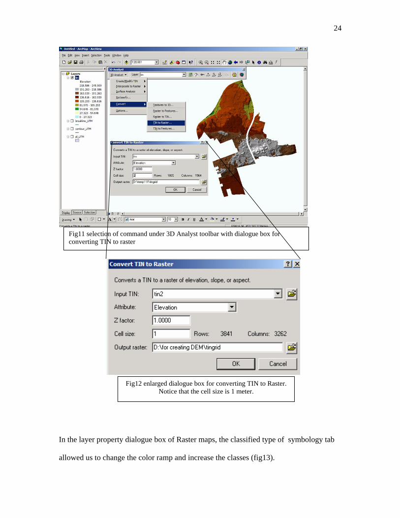
Fig11 selection of command under 3D Analyst toolbar with dialogue box for converting TIN to raster
Fig12 enlarged dialogue box for converting TIN to Raster. Notice that the cell size is 1 meter.
In the layer property dialogue box of Raster maps, the classified type of symbology tab
allowed us to change the color ramp and increase the classes (fig13).
25
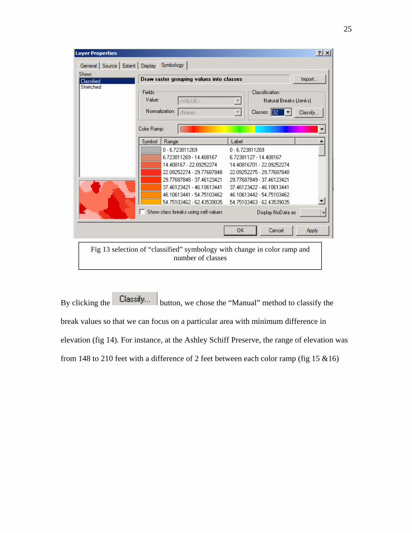
Fig 13 selection of “classified” symbology with change in color ramp and
number of classes
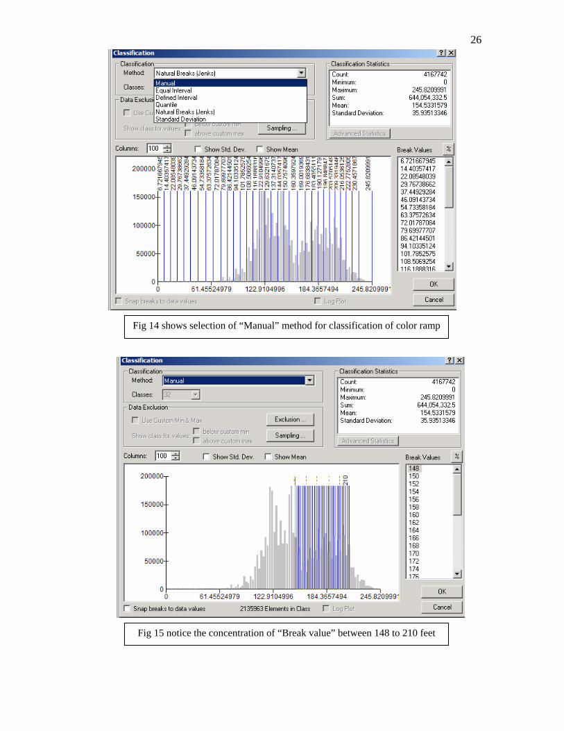
By clicking the button, we chose the “Manual” method to classify the
break values so that we can focus on a particular area with minimum difference in
elevation (fig 14). For instance, at the Ashley Schiff Preserve, the range of elevation was
from 148 to 210 feet with a difference of 2 feet between each color ramp (fig 15 &16)
26
Fig 14 shows selection of “Manual” method for classification of color ramp
Fig 15 notice the concentration of “Break value” between 148 to 210 feet
27
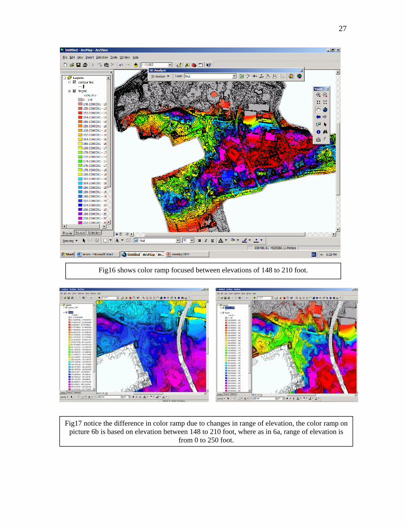
Fig16 shows color ramp focused between elevations of 148 to 210 foot.
Fig17 notice the difference in color ramp due to changes in range of elevation, the color ramp on
picture 6b is based on elevation between 148 to 210 foot, where as in 6a, range of elevation is from 0 to 250 foot.