Interpretational Applications of Spectral Decomposition

Greg Partyka, James Gridley, and John Lopez

Spectral Decomposition

• uses the discrete Fourier transform to:– quantify thin-bed interference, and– detect subtle discontinuities.

Outline

• Convolutional Model Implications• Wedge Model Response• The Tuning Cube• Spectral Balancing• Real Data Examples• Alternatives to the Tuning Cube• Summary

Long Window Analysis

• The geology is unpredictable.• Its reflectivity spectrum is therefore white/blue.

Long Window Analysis

Reflectivityr(t)

Fourier Transform

Amplitude

Fre

quen

cy

Waveletw(t)

Noisen(t)

Seismic Traces(t)

Amplitude Amplitude Amplitude

Fre

quen

cy

Fre

quen

cy

Fre

quen

cy

TIMEDOMAIN

FREQUENCYDOMAIN

Tra

vel T

ime

Short Window Analysis

• The non-random geology locally filters the reflecting wavelet.• Its non-white reflectivity spectrum represents the interference pattern

within the short analysis window.

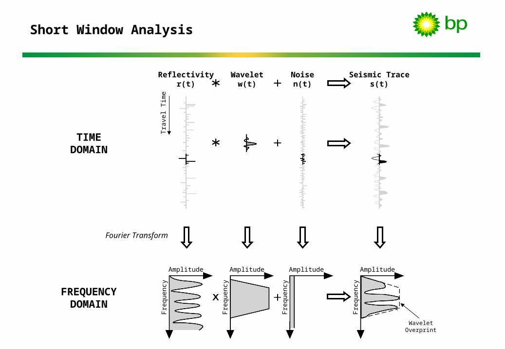
Short Window Analysis

WaveletOverprint

Reflectivityr(t)

Fourier Transform

Amplitude

Fre

quen

cy

Waveletw(t)

Noisen(t)

Seismic Traces(t)

Amplitude Amplitude Amplitude

Fre

quen

cy

Fre

quen

cy

Fre

quen

cy

TIMEDOMAIN

FREQUENCYDOMAIN

Tra

vel T

ime

Spectral Interference

• The spectral interference pattern is imposed by the distribution of acoustic properties within the short analysis window.

Spectral Interference

Source WaveletAmplitude Spectrum

Thin Bed ReflectionAmplitude Spectrum

Thin BedReflection

ReflectedWavelets

SourceWavelet

Thin Bed

ReflectivityAcousticImpedance

Temporal Thickness

FourierTransform

FourierTransform

Amplitude Amplitude

Fre

quen

cy

Fre

quen

cy

Temporal Thickness1

Outline

• Convolutional Model Implications• Wedge Model Response• The Tuning Cube• Spectral Balancing• Real Data Examples• Alternatives to the Tuning Cube• Summary

Wedge Model ResponseTemporal Thickness (ms)

REFLECTIVITY

FILTEREDREFLECTIVITY

(Ormsby 8-10-40-50 Hz)

SPECTRALAMPLITUDES

Temporal Thickness (ms)

Temporal Thickness (ms)

0 10 20 30 40 50

0 10 20 30 40 50

0 10 20 30 40 500

100

200

0

100

200

0

100

200

Tra

vel T

ime

(m

s)T

rave

l Tim

e (

ms)

Fre

qu

en

cy (

Hz)

Temporal Thickness1

Temporal Thickness

0.0015

0

Amplitude

Amplitude spectrum of 10ms blocky bedAmplitude spectrum of 50ms blocky bed10Hz spectral amplitude50Hz spectral amplitude

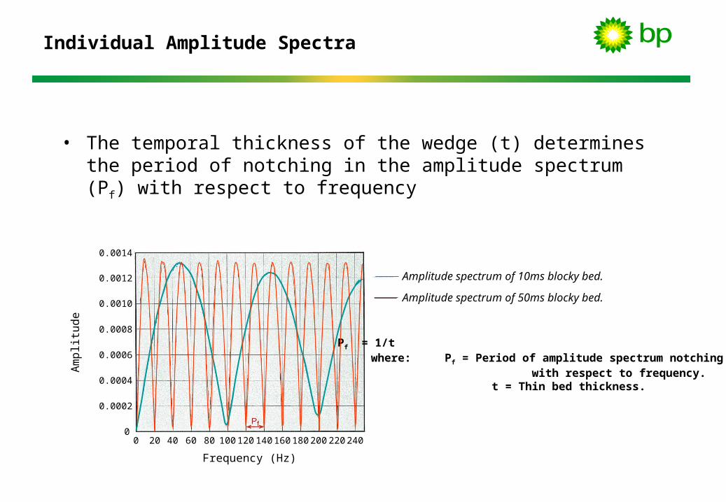
Individual Amplitude Spectra

Amplitude spectrum of 10ms blocky bed.

Amplitude spectrum of 50ms blocky bed.

Pf = 1/t where: Pf = Period of amplitude spectrum notching with respect to frequency. t = Thin bed thickness.

0 20 40 60 80 100 120 140 160 180 200 220 2400

0.0002

0.0004

0.0006

0.0008

0.0010

0.0014

0.0012

Frequency (Hz)

Am

plit

ud

e

• The temporal thickness of the wedge (t) determines the period of notching in the amplitude spectrum (Pf) with respect to frequency

Wedge Model ResponseTemporal Thickness (ms)

REFLECTIVITY

FILTEREDREFLECTIVITY

(Ormsby 8-10-40-50 Hz)

SPECTRALAMPLITUDES

Temporal Thickness (ms)

Temporal Thickness (ms)

0 10 20 30 40 50

0 10 20 30 40 50

0 10 20 30 40 500

100

200

0

100

200

0

100

200

Tra

vel T

ime

(m

s)T

rave

l Tim

e (

ms)

Fre

qu

en

cy (

Hz)

Temporal Thickness1

Temporal Thickness

0.0015

0

Amplitude

Amplitude spectrum of 10ms blocky bedAmplitude spectrum of 50ms blocky bed10Hz spectral amplitude50Hz spectral amplitude

Discrete Frequency Components

10Hz spectral amplitude.

50Hz spectral amplitude.

0 10 20 30 40 500

0.0002

0.0004

0.0006

0.0008

0.0010

0.0014

0.0012

Am

plit

ud

e

Temporal Thickness (ms)

Pt = 1/f where: Pt= Period of amplitude spectrum notching with respect to bed thickness. f = Discrete Fourier frequency.

• The value of the frequency component (f) determines the period of notching in the amplitude spectrum (Pt) with respect to bed thickness.

Outline

• Convolutional Model Implications• Wedge Model Response• The Tuning Cube• Spectral Balancing• Real Data Examples• Alternatives to the Tuning Cube• Summary

The Tuning Cube

xy

z

xy

z

xy

z

xy

freq

xy

freq

Interpret

3-D Seismic Volume

Subset

Compute

Animate

Interpreted3-D Seismic Volume

Zone-of-InterestSubvolume

Zone-of-InterestTuning Cube

(cross-section view)

Frequency Slicesthrough Tuning Cube

(plan view)

Outline

• Convolutional Model Implications• Wedge Model Response• The Tuning Cube• Spectral Balancing• Real Data Examples• Alternatives to the Tuning Cube• Summary

Prior to Spectral Balancing

• The Tuning Cube contains three main components:– thin bed interference,– the seismic wavelet, and– random noise

Multiply

Tuning Cube

xy

freq

xy

freqx

y

freqx

y

freq

Seismic Wavelet NoiseThin Bed Interference

++Add

Short Window Analysis

WaveletOverprint

Reflectivityr(t)

Fourier Transform

Amplitude

Fre

quen

cy

Waveletw(t)

Noisen(t)

Seismic Traces(t)

Amplitude Amplitude Amplitude

Fre

quen

cy

Fre

quen

cy

Fre

quen

cy

TIMEDOMAIN

FREQUENCYDOMAIN

Tra

vel T

ime

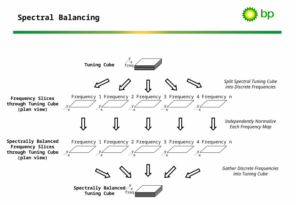
Spectral Balancing

xy

freq

xy

xy

xy

xy

xy

xy

xy

xy

xy

xy

xy

freq

Split Spectral Tuning Cubeinto Discrete Frequencies

Tuning Cube

Spectrally BalancedTuning Cube

Gather Discrete Frequenciesinto Tuning Cube

Independently NormalizeEach Frequency Map

Frequency 1 Frequency 2 Frequency 3 Frequency 4 Frequency n

Frequency 1 Frequency 2 Frequency 3 Frequency 4 Frequency n

Frequency Slicesthrough Tuning Cube

(plan view)

Spectrally BalancedFrequency Slices

through Tuning Cube(plan view)

After Spectral Balancing

• The Tuning Cube contains two main components:– thin bed interference, and– random noise

Tuning Cube

xy

freq

xy

freqx

y

freq

NoiseThin Bed Interference

+Add

Outline

• Convolutional Model Implications• Wedge Model Response• The Tuning Cube• Spectral Balancing• Real Data Examples• Alternatives to the Tuning Cube• Summary

Real Data Example

• Gulf-of-Mexico, Pleistocene-age equivalent of the modern-day Mississippi River Delta.

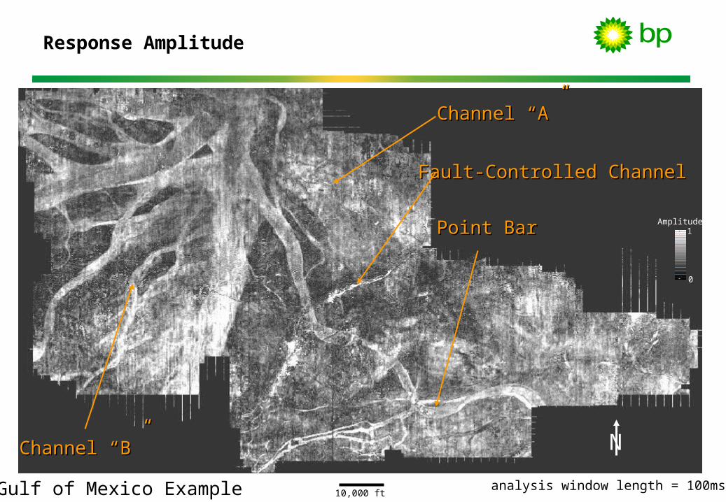
Gulf of Mexico Example 10,000 ft

Channel “A”Channel “A”

Channel “B”Channel “B”

Fault-Controlled ChannelFault-Controlled Channel

Point BarPoint Bar

N

1

0

Amplitude

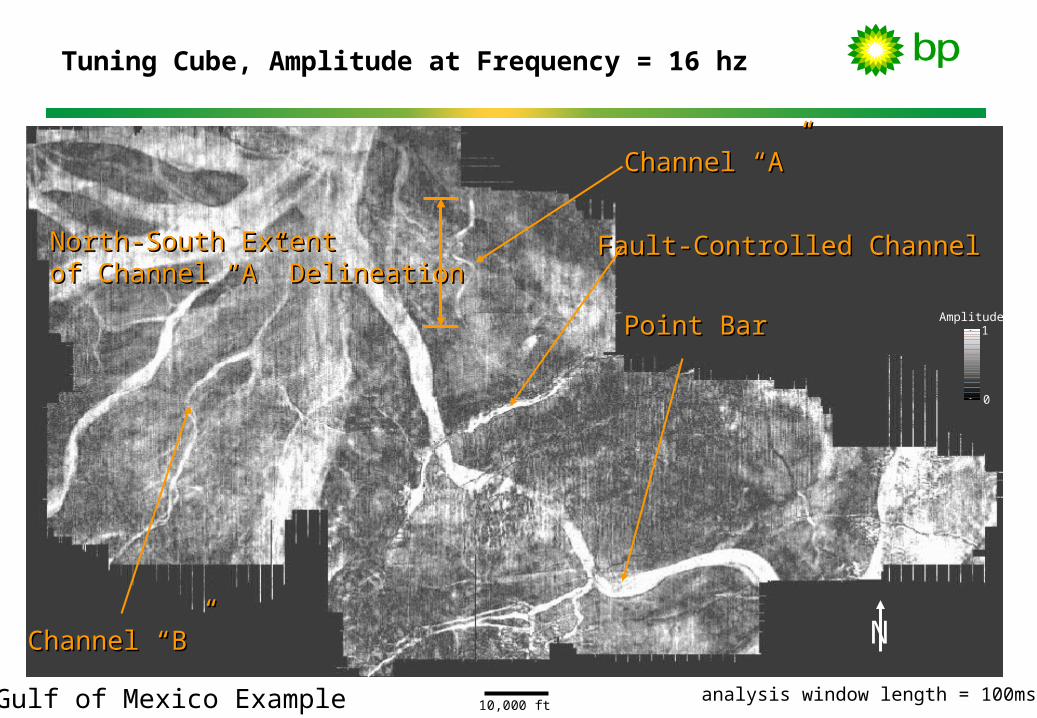
analysis window length = 100ms

Response Amplitude

Gulf of Mexico Example 10,000 ft

North-South ExtentNorth-South Extentof Channel “A” Delineationof Channel “A” Delineation

Channel “A”Channel “A”

Channel “B”Channel “B”

Fault-Controlled ChannelFault-Controlled Channel

Point BarPoint Bar

N

1

0

Amplitude

analysis window length = 100ms

Tuning Cube, Amplitude at Frequency = 16 hz

Gulf of Mexico Example 10,000 ft

North-South ExtentNorth-South Extentof Channel “A” Delineationof Channel “A” Delineation

Channel “A”Channel “A”

Channel “B”Channel “B”

Fault-Controlled ChannelFault-Controlled Channel

Point BarPoint Bar

N

1

0

Amplitude

analysis window length = 100ms

Tuning Cube, Amplitude at Frequency = 26 hz

Hey…what about the phase?

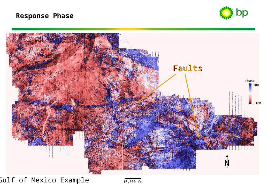
• Amplitude spectra delineate thin bed variability via spectral notching.• Phase spectra delineate lateral discontinuities via phase instability.

Phase Spectrum

Phase

Fre

quen

cy

Amplitude Spectrum

Amplitude

Fre

quen

cy

Thin Bed Reflection

FourierTransform

FaultsFaults

10,000 ft

N

180

-180

Phase

Gulf of Mexico Example

Response Phase

FaultsFaults

10,000 ft

N

180

-180

Phase

analysis window length = 100msGulf of Mexico Example

Tuning Cube, Phase at Frequency = 16 hz

analysis window length = 100ms

FaultsFaults

10,000 ft

N

180

-180

Phase

Gulf of Mexico Example

Tuning Cube, Phase at Frequency = 26 hz

Outline

• Convolutional Model Implications• Wedge Model Response• The Tuning Cube• Spectral Balancing• Real Data Examples• Alternatives to the Tuning Cube• Summary

Discrete Frequency Energy Cubes

Compute

3-D Seismic Volume

xy

freq

xy

freq

xy

freq

xy

freq

xy

freq

xy

freq

xy

freq

xy

z

z = 1

z = n

z = n

z = 3

z = 4

z = 5

z = 6

z = 1

z = 2

xy

z

z = 1

z = n

Subset

xy

z

z = 1

z = n

xy

z

z = 1

z = n

xy

z

z = 1

z = n

xy

z

z = 1

z = n

Time-Frequency 4-D Cube

Discrete FrequencyEnergy Cubes

Frequency 1 Frequency 2 Frequency 3 Frequency 4 Frequency m

Outline

• Convolutional Model Implications• Wedge Model Response• The Tuning Cube• Spectral Balancing• Real Data Examples• Alternatives to the Tuning Cube• Summary

Summary

• Spectral decomposition uses the discrete Fourier transform to quantify thin-bed interference and detect subtle discontinuities.

• For reservoir characterization, our most common approach to viewing and analyzing spectral decompositions is via the “Zone-of-Interest Tuning Cube”.

• Spectral balancing removes the wavelet overprint.• The amplitude component excels at quantifying thickness variability

and detecting lateral discontinuities.• The phase component detects lateral discontinuities.