Embed Size (px)
Citation preview
1949-3045 (c) 2020 IEEE. Personal use is permitted, but republication/redistribution requires IEEE permission. See http://www.ieee.org/publications_standards/publications/rights/index.html for moreinformation.
This article has been accepted for publication in a future issue of this journal, but has not been fully edited. Content may change prior to final publication. Citation information: DOI10.1109/TAFFC.2020.3035535, IEEE Transactions on Affective Computing
IEEE TRANSACTIONS ON AFFECTIVE COMPUTING, VOL. X, NO. X, JANUARY 2020 1
Interpretation of Depression Detection Modelsvia Feature Selection Methods
Sharifa Alghowinem, Tom Gedeon, Senior Member, IEEE, Roland Goecke, Senior Member, IEEE, JeffreyF. Cohn, and Gordon Parker
Abstract—Given the prevalence of depression worldwide and its major impact on society, several studies employed artificialintelligence modelling to automatically detect and assess depression. However, interpretation of these models and cues are rarelydiscussed in detail in the AI community, but have received increased attention lately. In this study, we aim to analyse the commonlyselected features using a proposed framework of several feature selection methods and their effect on the classification results, whichwill provide an interpretation of the depression detection model. The developed framework aggregates and selects the most promisingfeatures for modelling depression detection from 38 feature selection algorithms of different categories. Using three real-worlddepression datasets, 902 behavioural cues were extracted from speech behaviour, speech prosody, eye movement and head pose. Toverify the generalisability of the proposed framework, we applied the entire process to depression datasets individually and whencombined. The results from the proposed framework showed that speech behaviour features (e.g. pauses) are the most distinctivefeatures of the depression detection model. From the speech prosody modality, the strongest feature groups were F0, HNR, formants,and MFCC, while for the eye activity modality they were left-right eye movement and gaze direction, and for the head modality it wasyaw head movement. Modelling depression detection using the selected features (even though there are only 9 features) outperformedusing all features in all the individual and combined datasets. Our feature selection framework did not only provide an interpretation ofthe model, but was also able to produce a higher accuracy of depression detection with a small number of features in varied datasets.This could help to reduce the processing time needed to extract features and creating the model.
Index Terms—depression detection, multimodal analysis, feature selection, datasets generalisation.
F
1 INTRODUCTION
A CCORDING to the World Health Organisation (WHO), majordepressive disorders are an increasing global issue that leads
to devastating consequences [1]. A person living with depressionsuffers enormously and functions poorly in everyday life tasks.Depression is a major contributor to the overall global burdenof disease and is the leading cause of disability worldwide.Depression is strongly linked with non-communicable disorders,such as diabetes and heart disease, increased risk of substance usedisorders, and at its worst, it can lead to suicide. Even thoughtreatments for depression are effective, only 10% of depressedpatients receive such treatments, where one of the barriers toeffective care is inaccurate diagnoses. Misdiagnosed and untreateddepression does not only affect the sufferer at a personal level, butalso affects the employer and the government at an economic level.
Given the prevalence of depression disorder worldwide andits major impact, several studies attempted to automatically detectand diagnose depression by employing artificial intelligence mod-elling. Modelling depression in these studies varied in terms of
• S. Alghowinem is with Media Lab, Massachusetts Institute of Technology,Cambridge, MA, USA, with Prince Sultan University, Riyadh, Saudi Arabiaand with the Australian National University, Canberra, AustraliaE-mail: [email protected]
• T. Gedeon is with the Australian National University, Canberra, Australia.E-mail: [email protected]
• R. Goecke is with the University of Canberra, Canberra, AustraliaE-mail: [email protected]
• J.F. Cohn is with the University of Pittsburgh, Pittsburgh, PA, USA.E-mail: [email protected]
• G. Parker is with the University of New South Wales, Sydney, Australia.E-mail: [email protected]
investigated modalities, extracted features, modelling algorithms,etc. Moreover, depression datasets collected by these studies arealso different in purpose, procedure, and environment. The use ofmodelling algorithms with such diverse modalities and their highdimensional feature spaces, restricts the ability to interpret its re-sults. Moreover, such differences prevent generalisation and draw-ing solid conclusions about the effectiveness of the modelling.Feature selection techniques aim at reducing the dimensionalityof the feature space in order to increase the efficiency of themodelling. However, the majority of such techniques focus onreducing the number of features used to select the features withhighest class discriminative power, without giving an insight intowhat features are being selected. Similarly, depression detectionmodelling studies that used feature selection methods did not pro-vide the selected features by these techniques, which is importantto interpret and generalise a model to other datasets.
To improve the interpretability and generalisability of depres-sion analysis modelling, we investigate a novel and robust frame-work that aggregates the results from different feature selectionmethods. That is, we utilise several feature selection methodsto interpret a depression detection model, and analyse their ef-fect on the classification and generalisation results. We extractbehavioural and functional features from speech, eye activitiesand head movement from three depression datasets. By having acloser look at the features being selected by the feature selectionmethods, we hypothesise that; (1) there are features that arecommonly selected by feature selection methods that stronglydistinguish depressed behaviour, (2) that these commonly selectedfeatures are robust to randomness and are consistently selectedwithin different thresholds of the same feature selection method,and (3) finding these features can be helpful for generalisable
Authorized licensed use limited to: Australian National University. Downloaded on January 27,2021 at 05:45:51 UTC from IEEE Xplore. Restrictions apply.
1949-3045 (c) 2020 IEEE. Personal use is permitted, but republication/redistribution requires IEEE permission. See http://www.ieee.org/publications_standards/publications/rights/index.html for moreinformation.
This article has been accepted for publication in a future issue of this journal, but has not been fully edited. Content may change prior to final publication. Citation information: DOI10.1109/TAFFC.2020.3035535, IEEE Transactions on Affective Computing
IEEE TRANSACTIONS ON AFFECTIVE COMPUTING, VOL. X, NO. X, JANUARY 2020 2
modelling of depression behaviour independent of the datasetsand recording process.
To best of our knowledge, this paper is the first to explore anextensive array of feature selection methods to find the strongestfeatures for a depression diagnosis. The novelty of this paper is asfollows:
• We perform a comprehensive analysis of feature selectiontechniques in the context of depression behaviour fromdifferent family groups of feature selection techniques;traditional flat feature, dynamic (streaming) feature, andstructural based feature selection techniques.
• We propose a framework to aggregate the results of thefeature selection techniques to increase the robustnessto randomness of the selected features, using differentstability measures. We also propose a new feature selectionstability measure using between thresholds stability.
• We generalise the framework by applying it on differ-ent depression datasets to select the more representativefeatures. Then, we investigate the effectiveness of thesefeatures by creating depression severity models usingdifferent depression datasets.
This exploration facilitates the interpretation of depression be-haviour since it is applied on a clinically annotated matchedcontrol-depressed database using multimodal behavioural analy-sis. Identifying the most meaningful depression behaviour patternsis significant since behaviour has been associated with depression-related symptoms in psychology literature. For this purpose,the main contribution of this paper is the extensively validatedframework that not only reliably identified the characteristicsof depression behaviour, but also provided an understanding ofrecognition model performance and its generalisability.
2 RELATED WORK
Automatic modelling of depression aims at providing an objectivemeasure for a depression diagnosis. This approach addresses theissue of misdiagnosing depression, which is considered one of themain barriers to depression treatments. These studies investigatedseveral cues of depression analysis including; facial expression,speech characteristics, head and body movement, brain signals,linguistic choices for text and speech, etc. The extracted featuresfrom such studies differ between each other even when analysingthe same modality, as well as machine learning techniques usedin these studies varies. Intensive reviews of these studies are pre-sented in [2] for visual features and [3] for speech features. Recentresearch on depression modelling share the same differences.
For example, with the emergence of deep learning techniques,[4] utilised deep convolutional neural networks (DCNN) to modeldepression diagnosis from facial expression. They used facialappearance and dynamic facial movement as images to fine-tunetwo separate pre-trained DCNNs, then fused their results in score-fusion level. The results of their networks architecture outperformthose of other studies. However, due to the complexity of deeplearning techniques, it is difficult to interpret the features that con-tributed to such improvement in the performance. Moreover, deeplearning techniques need a huge number of labelled observations.Therefore, it is common to use pre-trained networks. In that study,the pre-trained sample was of a general face recognition dataset.This might have an effect on the diagnosis of depression.
Another study modelled forecasting depression mood based onself-reported history using a recurrent neural network (RNN) [5].
The study used long-term historical information of a user that in-cludes; user reported mood, action, medications, sleeping patterns,etc. The subjects of the study report the information periodicallyeach day over several months. The study could accurately forecastsevere depression mood up to two weeks in advance. However,since the information is self-reported, there is no indication ofhow such a model would work as an automated system.
Another example of deep learning utilisation for depressiondetection is presented in [6], where audio and text features areextracted from virtual agent-human interaction interviews. A long-short-term memory (LSTM) neural network model is built usingaudio and text features, where it outperformed the baseline result.Although, it is difficult without further investigation to interpretthe model to know exactly what features contributed to the highperformance.
Using AVEC dataset, [7] investigated three deep learningtechniques as a method of transferred learning in an effort toincrease the diagnosis of depression severity based on visualcues. Even though their results show similarity to the state-of-the-art, it does not provide an interpretation of the model and itseffectiveness.
Even without using deep learning, automatic feature extractionfrom video signal are not always interpretable. For example, in[8], dynamic facial feature descriptors are automatically extractedfrom the video recording of AVEC depression dataset. Localbinary pattern is extracted from three orthogonal planes to capturemicrostructure of facial appearance, where the results histogramsare concatenated. Fisher vector is then used to cluster the features,and a support vector regression is used for depression severitymodelling. The results showed an improvement from the baselineand other studies. However, such approaches are difficult tointerpret.
Feature selection methods have been utilised for depressionmodelling studies, with the goal of improving the accuracy ofdepression diagnosis. Both survey papers of [2] and [3] listed somestudies that utilised feature selection methods. However, suchstudies do not report the selected feature set, which would improvethe understanding of the generalisation of their findings, nor reportstability measures and the procedure to increase it. Moreover,some of these studies used feature transformation methods, wherethe actual features that contribute to the modelling cannot beidentified.
For example, in [9], depression diagnosis was investigatedusing facial dynamic analysis, where extracted features weretransformed using sparse coding. Sparse coding aims at reducingthe complexity of dynamic features and aims at suppressing thenoise in a feature. Sparse coding is a compression method similarto feature transformation, where the original features after thecoding cannot be identified. Likewise, in [10], where they usedPrincipal Component Analysis (PCA), a feature transformationmethod, for dimensionality reduction of acoustical and perceptualspeech features to detect depression. In [11], non-linear down-sampling function for dimensionality reduction was applied onspeech. Even though [12] employed both transformation methodand a voted version of correlation-based as a filter feature selectionmethod, the selected features based on the filter method were notreported.
Sharing a similar goal of model interpretation as this currentwork, [13] recently developed a method to measure depressionseverity automatically using face and head modalities. The facialfeatures (shape representation) were isolated from head movement
Authorized licensed use limited to: Australian National University. Downloaded on January 27,2021 at 05:45:51 UTC from IEEE Xplore. Restrictions apply.
1949-3045 (c) 2020 IEEE. Personal use is permitted, but republication/redistribution requires IEEE permission. See http://www.ieee.org/publications_standards/publications/rights/index.html for moreinformation.
This article has been accepted for publication in a future issue of this journal, but has not been fully edited. Content may change prior to final publication. Citation information: DOI10.1109/TAFFC.2020.3035535, IEEE Transactions on Affective Computing
IEEE TRANSACTIONS ON AFFECTIVE COMPUTING, VOL. X, NO. X, JANUARY 2020 3
using barycentric coordinates. They also extract head movement,where they used feature reduction on the two modalities such asPCA and mRMR (minimum Redundancy Maximum Relevance).The face and head movement were presented as a histogramto interpret the results, where the velocity features of facialshape representation show strong discrimination power with re-spect to depression severity. To further this line of research oninterpretability, we analyse depression modelling from featuresextracted from speech behaviour, speech prosody, eye activity aswell as head movement in a multimodal manner.
3 BACKGROUND ON FEATURE SELECTION
In general, feature selection methods are categorised to supervised,when the classes’ labels are known and used to evaluate thefeatures, and unsupervised, when no labels are available andfeatures are clustered and evaluated for redundancy. This workutilises supervised feature selection methods only, since the focushere is supervised depression detection modelling. Supervisedfeature selection techniques aim at finding small and representativefeatures that differentiate classes from each other. This is done byremoving redundant features and features that do not add value todistinguish the classes.
There are several categorisations for feature selection methods,which are based on their applications, input and output datatypes (see Table 1). For example, feature selection methods thatevaluate all extracted features at once are under flat (static) featurecategory, while feature selection methods that evaluate each ex-tracted feature as they come available (e.g. online streaming) areunder dynamic feature category. Flat feature selection methodsare traditionally employed in the literature, where their algorithmsassumes that the features are known and extracted in advance.Dynamic feature selection methods are excellent when the totalnumber of features are not known in advance, and they evaluatethe new feature to decide (depending on the algorithm) to eitherinclude it, replace an old feature with the new one or ignore it.Even though the feature space in our investigation is known inadvance, we also chose to apply the dynamic feature selection asan approach to analyse the selected features by these methods.Another family of feature selection methods deals with structuraldata, where relations between features are learned to construct astructure (e.g. tree), and then the selected features will be basedon their location in the structure (e.g. a feature that is located inhigher nodes of a tree are more likely to be selected than one inan isolated branch of the tree).
Regardless of the categorisations, every feature selectionmethod uses a different technique/algorithm to evaluate the fea-tures. Some feature selection techniques evaluate each featureindividually and their contribution in distinguishing the classeswithout considering the relationship with other features (e.g. t-score). Other techniques evaluate the correlation of features withthe class and each other (e.g. Correlation Feature Selection (CFS)).Some techniques evaluate feature groups instead of individualfeatures, where the feature group as a whole is evaluated forselection.
Moreover, feature selection techniques/algorithms differ in thetype of input features to be evaluated, where some methods onlyevaluate discrete input data, while others evaluate both continuousand discrete input data. Based on the output of the method, featureselection methods can be categorised to ranking features, scoringfeatures and selecting feature subset. Ranking methods sort the
features based on their importance and value in distinguishingthe classes. Scoring methods output a score for each featurerepresenting their importance, such that the higher the feature’sscore the higher its value in separating the classes. On the otherhand, methods that output a feature subset do not give a score ora ranking to individual features, rather they produce a subset offeatures that performs better in classifying the classes.
For dynamic feature selection, Scalable and Accurate OnlineFeature Selection (SAOLA) [14] and group-SAOLA [15] wereproposed as an online pairwise comparison with a focus onscalability solutions. Relevancy and redundancy of features areanalysed using mutual information for the decision of includingor excluding them. A continuous comparison between the previ-ously selected features and the newly arrived feature, where thefeature with lower relevance with the target class is removed.In the group-SAOLA algorithm, features are divided into groups(e.g. for image analysis, feature groups like SIFT features andcolour and shape features [15]), and within each group, severalindividual features exist. The individual features in a group areanalysed first, where redundant and irrelevant features within thatgroup are removed. Then the remaining features from differentgroups are analysed, where redundant features from other groupsare removed. Online Streaming Feature Selection (OSFS) [16]and fast-OSFS [17] also use mutual information in verifyingthe relevance and redundancy of features. Alpha-investing is astreaming feature selection method that uses statistical criterionto analyse the relevancy of newly arrived features [18]. Alpha-investing dynamically adjusts a threshold on the p-statistic tocontrols adding a new feature to the model. That is, if the p-value of a new feature is greater than the threshold, then thefeature is added to the model. In Alpha-investing, OSFS and fast-OSFS methods, once a feature is selected it will not be removed.Instead, the new arriving feature will be evaluated for inclusionbased on its relevance to the class and its redundancy to alreadyselected features. The above dynamic methods use a α-statisticalsignificance level to determine the inclusion of a new feature.Alpha-investing uses dynamically adjusted α, while the others usea predefined α for inclusion, where in this work it is set to 0.1.Adaptive group LASSO (AGLasso) (least absolute shrinkage andselection operator) was proposed to overcome inconsistency inselecting features from LASSO and group LASSO. The LASSOmethod applies a shrinking (regularisation) process by penalisingthe coefficients of the variables, where only the variables withnon-zero coefficient are selected. LASSO uses the l1 penalisedleast squares criterion to evaluate features, which is the sum ofthe coefficients’ absolute values. As a result, many coefficientswill be zeroed under LASSO with high values of a threshold(selected in advance). Adaptive group LASSO has flexibilitythrough weighting each coefficient differently to avoid applyingthe same penalty, which could result in over and insufficientlyshrinking regression coefficients.
Some feature selection methods learn a structure from theanalysed features to select the best features, including network,tree, and graph structures, as well as rough sets. Unlike mosttraditional methods that are limited to find interactions betweenfew variables, structure data methods capture high-order interac-tions between the variables. To learn a network structure frominput features, Bayesian Network using Markov Blanket (MB)is widely used. We chose two methods from this group namelythe traditional max-min parent children MB (MM-MB) [19] andstate-of-the-art statistically equivalent signature (SES-MB) [20].
Authorized licensed use limited to: Australian National University. Downloaded on January 27,2021 at 05:45:51 UTC from IEEE Xplore. Restrictions apply.
1949-3045 (c) 2020 IEEE. Personal use is permitted, but republication/redistribution requires IEEE permission. See http://www.ieee.org/publications_standards/publications/rights/index.html for moreinformation.
This article has been accepted for publication in a future issue of this journal, but has not been fully edited. Content may change prior to final publication. Citation information: DOI10.1109/TAFFC.2020.3035535, IEEE Transactions on Affective Computing
IEEE TRANSACTIONS ON AFFECTIVE COMPUTING, VOL. X, NO. X, JANUARY 2020 4
The main difference between MM-MB and SES-MB is that thelatter extends the first by finding multiple subsets of feature thathave statistically equivalent performances. Both methods utiliseBayesian networks as graphical models in order to give compactrepresentations of multivariate distributions. The graph composedof nodes that represent variables, and edges that represent relationsbetween the variables, either parent or child. MB is derived basedon the parent, children, and any additional parent of children(spouses) of a node. MB of a feature finds redundant features to beeliminated, while MB of a target class comprises a set of selectedfeatures. In SES-MB, it is assumed that multiple MBs exists fora target class, where the best representative set is determined forfinal selection.
Tree structure using random forest variations has been alsoutilised for feature selection, where five methods were used in thiswork. A random forest (RF) is used to measure feature importance[21], where the features with the highest importance scores areselected individually. However, this approach does not considerfeature redundancy. Regularised RF (RRF) recursively split data,then penalise selecting a new feature that has similar gain (e.g.information gain) to the features used in previous splits [22].Guided RRF (GRRF) method employs ordinary RF to guide RRFfor selecting the features based on feature importance scores [23].Selection of grouped variables using random forests was proposed(GRF), where permutation-based importance measure is used foreach feature group [24]. A most recent approach used GradientBoosting for feature selection [25], where sequential trees are usedfor learning and regularised by LASSO.
Graph-based feature selection offers similar benefits of struc-tured data, where the problem feature selection is mapped to anaffinity graph (features are the nodes). Infinite Feature Selection(Inf-FS) finds a path in the graph that connects a subset of featuresto evaluate the importance of each feature while consideringall the possible subsets of features [26]. Infinite Latent FeatureSelection was proposed as an extension of Inf-FS, where rele-vancy is modelled as a latent variable [27]. Similarly, EigenvectorCentrality (EigenC) assesses the importance of a feature based onits centrality and the importance of its neighbours [28].
Rough set theory (RST) has been used for feature selection forits ability to deal with incomplete knowledge. In feature selection,RST finds a reduct set of attributes, which is a set of featuresthat have high accuracy in classification. Several algorithms areused to find the reduct. Quick Reduct is a well-known methodthat uses a greedy search algorithm to select a subset of featuresusing dependency degree as stopping criteria [29]. DynamicallyAdjusted Approximate Reducts (DAAR) modifies Quick Reductmethod by including an additional stop condition, which is arandom permutation [30]. The near-optimal (nearOpt) implementsfast heuristic algorithms to obtain one near-optimal attribute re-duction instead of finding all reducts [31].
Traditional feature selection assumes a flat (static) and knownin advance predictors. Flat feature selection are categorised tofilter, embedded and wrappers, where the well-known and widelyused methods in the literature are employed in this work. Filtermethods use statistical (e.g. t-score [32], Chi square [33], CFS[34]), similarity (e.g. Fisher score [35], ReliefF [36], SpectralFeature Selection (SPEC) [37]) and information theory approaches(e.g. mRMR [38], Joint Mutual Information (JMI) [39], Condi-tional Mutual Information Maximisation (CMIM) [40], DoubleInput Symmetrical Relevance (DISR) [41]) to select the best fea-tures. While embedded (e.g. LASSO [42], L1-SVM [43], Elastic
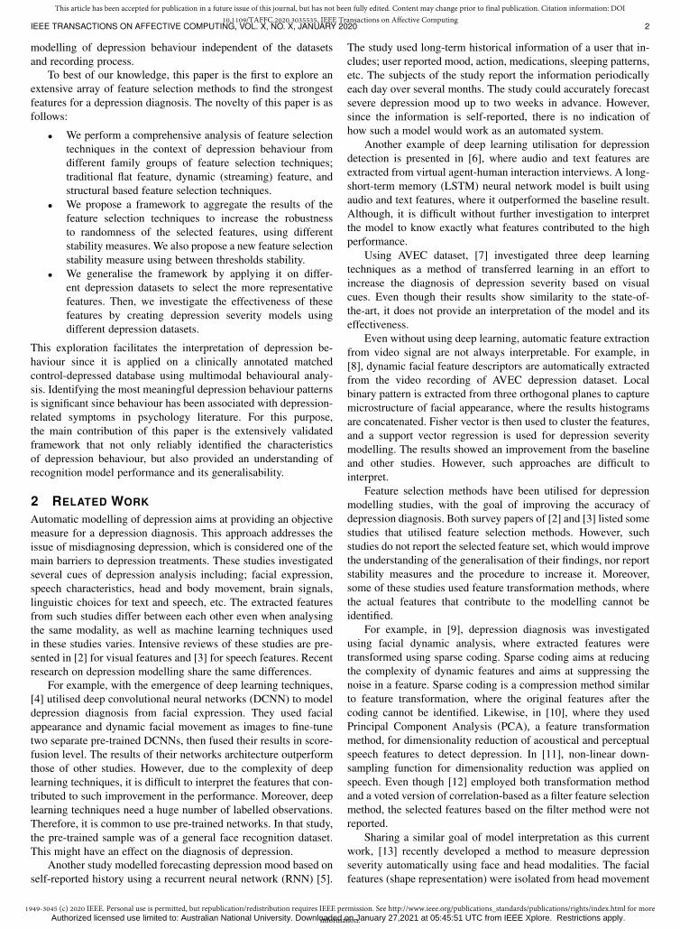
Fig. 1: Preparation Phase of the Feature Selection Framework
Nets [44], Ridge [45]) and wrappers (e.g. genetic algorithms (GA)[46], Boruta [47], conditional covariance minimisation (CCM)[48], recursive feature elimination with a linear SVM (SVM-RFE)[49], SVM-Backward feature selection [50]) employs classifica-tion algorithms for evaluations.
4 SELECTING FEATURE FRAMEWORK
In this section, we introduce our proposed feature selectionframework for the interpretation and classification of depressiondetection model. Our proposed framework for feature selectioncomprise of three main phases, preparation phase (see Figure 1),feature selection process phase (see Algorithm 1), and aggregationphase (see Figure 3).
4.1 Preparation PhaseThe steps in the preparation phase start with collecting videorecording of subjects (depressed and control). The raw videorecording is analysed to extract several behavioural features fromdifferent modalities. A variety of feature selection algorithms fromdifferent families are implemented to be applied to the extractedfeatures.
4.1.1 Depression DatasetsThe main dataset used in this work is a real-world data collectedin an ongoing study at the Black Dog Institute, as detailed in [51].For the generalisation purposes, we used two other depressiondatasets, University of Pittsburgh depression dataset (Pitt) [52]and Audio/Visual Emotion Challenge Depression Dataset (AVEC)[53].
BlackDog: The Black Dog Institute is a clinical research facil-ity in Sydney, Australia, offering specialist expertise in depressivedisorders. Only subjects who fit the criteria of healthy controls,as well as depressed patients, are included. All depressed subjectsmet the DSM-IV (Diagnostic and Statistical Manual of MentalDisorders - fourth edition) criteria for either moderate or severedepression. Quick Inventory of Depressive Symptomatology self-report (QIDS-SR) [54] was used to score the severity of depres-sion, (QIDS-SR score of 11-15 points refer to a “Moderate” level,16-20 points to a “Severe” level, and ≥ 21 points to a “VerySevere” level). Control participants were also screened for historyof psychiatric and neurological illness. Once subjects were foundto meet the inclusion criteria, they are invited to undergo theexperimental paradigm.
Authorized licensed use limited to: Australian National University. Downloaded on January 27,2021 at 05:45:51 UTC from IEEE Xplore. Restrictions apply.
1949-3045 (c) 2020 IEEE. Personal use is permitted, but republication/redistribution requires IEEE permission. See http://www.ieee.org/publications_standards/publications/rights/index.html for moreinformation.
This article has been accepted for publication in a future issue of this journal, but has not been fully edited. Content may change prior to final publication. Citation information: DOI10.1109/TAFFC.2020.3035535, IEEE Transactions on Affective Computing
IEEE TRANSACTIONS ON AFFECTIVE COMPUTING, VOL. X, NO. X, JANUARY 2020 5
Participants, both depressed and control, are audio-videorecorded in one session only. The audio-video experimentalparadigm contains several parts, including answering open-endedquestions. The interview is conducted by asking specific open-ended questions, where the subjects are asked to describe eventsin their life that had aroused significant emotions. This item isdesigned to elicit spontaneous, self-directed speech and relatedfacial expressions, as well as overall body language.
In this work, a gender-balanced subset of 30 depressed subjectsand 30 controls were used for the analysis. For depressed subjects,the level of depression was a selection criterion, with a mean of19 points (range 14-26 points) of the diagnoses using QIDS-SRscores. Even though the sample size used here is relatively small,this is a common problem in similar clinically validated datasets.Furthermore, from the parts of the experimental paradigm, onlythe interview section was analysed for feature extraction.
Pitt: The data are from a subset of 57 participants in a clinicaltrial for treatment of depression conducted at the University ofPittsburgh Medical Center. Treatment consisted of antidepressantmedication (i.e., an SSRI) or interpersonal psychotherapy [52].Both are evidence-based treatments for depression.
All participants met DSM-IV criteria for Major DepressiveDisorder (MDD) at start of the study. Audio-video recordingswere obtained during depression severity interviews at 7-weekintervals over 21 weeks beginning at week one. HRSD (HamiltonRating Scale for Depression) scores of 15 or higher are generallyconsidered to indicate moderate to severe depression; and scoresof 7 or lower to indicate a return to normal [55].
Nineteen participants scored 7 or below at one or moresessions. For inclusion in the study, we randomly sampled onelow-depression session from each of these participants. We thenrandomly sampled a session rated as severe from among an equalnumber of randomly selected participants that scored in the severerange. Thus, the final sample consisted of 38 participants: 19 witha low-depression session and 19 with a severe-depression session.
AVEC: The Audio/Visual Emotion Challenge (AVEC) is asubset of the German audio-video depressive language corpus(AVDLC). In its 2013/2014 versions, AVEC included a challengeon an automatic estimation of depression level [53]. The databaseincludes 340 video clips of 292 subjects, with only one person perclip, i.e. some subjects feature in more than one clip. The speakerswere recorded between one and four times, with a period of twoweeks between the measurements. However, in this work we onlyselect one session per subject, where the subjects from the severeand low depression do not cross.
In AVEC dataset, the depression severity is based on the BeckDepression Index (BDI), which is a self-reported 21 multiplechoice inventory [56]. The BDI scores range from 0 to 63, where0-13 indicates minimal depression, 14-19 indicates mild depres-sion, 20-28 indicates moderate depression, and 29-63: indicatessevere depression. The average BDI-level in the AVEC datasetwas 15 points (standard deviations = 12.3).
The AVEC depression database contains naturalistic video andaudio of participants partaking in a human-computer interactionexperiment guided by PowerPoint and contains several tasksincluding telling a story from the subject’s own past (i.e. bestgift ever and sad event in childhood).
In this paper, a balanced subset of AVEC database is selectedbased on the BDI score. We categorised the recordings in binarygroups indicating severe-depressed where BDI score is more than29, and minimal-depressed where BDI score is less than 13. Since
there were only 16 subjects with a BDI score more than 29, thesame number of subjects is selected with ascending low BDIscore from 0 to 4. The spontaneous childhood storytelling fromthe recording tasks is analysed for feature extraction, in order tomatch the spontaneous interview from BlackDog and Pitt datasets.
As can be seen, the datasets differ in aim, depression assess-ment/scoring method, and recording procedure. BlackDog aims tocompare depressed patients with healthy controls, while both Pittand AVEC datasets measure and monitor depression severity. Eachdataset used different depression assessment tools, which made thedepression scores incomparable. In BlackDog and Pitt datasets,all depressed subjects met DSM-IV criteria initially. In BlackDog,depression was assessed using QIDS-SR from both depressed andcontrol subjects. In Pitt, depressed subjects were classified bytheir subsequent score on a depression severity interview (HRSD,which is the gold standard in clinical trials). In AVEC, all subjectswere assessed using a cut-score on the self-report BDI. Thesemethods correspond to the various ways that depression is assessedin research and clinical practice. For consistency across the threedatasets, each of the respective scores was converted to its QIDS-SR equivalent using the conversion table from [57]. Each datasetis treated and classified as a binary classification task. That is, withBlackDog dataset the system classifies depressed from controlsubjects, while with Pitt and AVEC the system classifies severedepression from low depression.
4.1.2 Modalities and Feature ExtractionBehavioural patterns (using statistical measures) of subjects’ re-sponses during the interview (interaction) were extracted fromdifferent modalities, which are; speech behaviour, speech prosody,eye activity, and head movement. Given the differences not onlybetween subjects, but also between dataset recording environ-ments, normalising each extracted feature was performed within-subject session as described below, and listed in Table 4.
Speech behaviour (SB) (for BlackDog only) Verbal cuesand interaction style observed during clinical interviews showedsignificant differences between depressed and control subjects[58]. Recently, [59] found that speech behaviour features (e.g.speakers’ turns, laughter) performed better than other modalities’features (e.g. speech prosody, visual features) in depression sever-ity modelling. The speech interaction pattern during interviews isextracted, following the methodology in [51], (which was donefor the BlackDog dataset only due to differences on the otherdatasets). For the BlackDog dataset, the interviews were manuallylabelled to separate speakers (i.e., research assistant (RA) and thesubject) and to separate several parts of the speech signal foranalysis. A total of 88 speech behaviour features are extracted,where these features are grouped listed below. For each featuregroup, 9 statistical measures are calculated including the average,maximum, minimum, range, variance, standard deviation, total,rate, and frequency of occurrence.
Speech prosody (SP): A recent review on the utilisation ofspeech prosody features in modelling depression detection anddepression severity showed a great impact of these features inthe accuracy of the model [3]. Statistical functionals from low-level prosody features were extracted from sounding segments,following the procedure in [60], where the raw features areextracted with frame size set to 25ms at a shift of 10ms andusing a Hamming window. The most common features in thedepression detection literature from the fields of psychology andaffective computing were extracted as listed in the feature groups
Authorized licensed use limited to: Australian National University. Downloaded on January 27,2021 at 05:45:51 UTC from IEEE Xplore. Restrictions apply.
1949-3045 (c) 2020 IEEE. Personal use is permitted, but republication/redistribution requires IEEE permission. See http://www.ieee.org/publications_standards/publications/rights/index.html for moreinformation.
This article has been accepted for publication in a future issue of this journal, but has not been fully edited. Content may change prior to final publication. Citation information: DOI10.1109/TAFFC.2020.3035535, IEEE Transactions on Affective Computing
IEEE TRANSACTIONS ON AFFECTIVE COMPUTING, VOL. X, NO. X, JANUARY 2020 6
below. Following the literature, and to increase the accuracy ofdepression detection, the first (∆) and second (∆∆) derivativesof each low-level feature were also extracted [3]. Then a total of504 statistical functional features are calculated in session-level,where 6 statistical measures are extracted for each feature andits ∆s derivatives that include mean, minimum, maximum, range,variance and standard deviation.
Eye activity (EB): Eye movements of depressed patientstudies were reviewed in [61], where such features were shownto have statistical discriminating power between patients withdepressive disorders from controls. Such features were also usedfor modelling depression detection, where they show promisingresults [62]. Following the methodology of eye feature extractionin [63], eye activity (e.g. blinking, iris movement) were extractedusing eye detection and tracking model, for each eye in each frame(25 fps). A total of 126 statistical features (average, maximum,minimum, variance, and standard deviation) of the feature and its∆s derivatives were extracted and grouped as listed in Table 4.
Head movement (HB): Studies on depressed patients’ be-haviour demonstrated a pronounced nonverbal behaviour includ-ing head movement that reflects depression persistence [64].Modelling depression detection using head gesture and movementshowed supporting results to other cues [65]. Following the pro-cedure in [63], we extract 3 degrees of freedom head movementbehavioural patterns from each frame (25 fps). From these posefeatures, as well as their velocity and acceleration (∆s derivatives),we extract a total of 184 statistical features as grouped below. Thestatistical measures include maximum, minimum, range, mean,variance, and standard deviation for the features, its derivatives,and their changes, as well as maximum, minimum, range, average,and rate of head direction duration
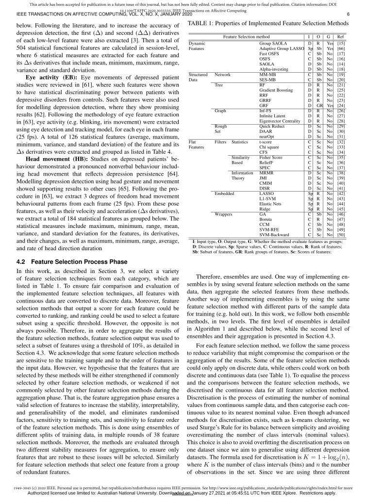
4.2 Feature Selection Process PhaseIn this work, as described in Section 3, we select a varietyof feature selection techniques from each category, which arelisted in Table 1. To ensure fair comparison and evaluation ofthe implemented feature selection techniques, all features withcontinuous data are converted to discrete data. Moreover, featureselection methods that output a score for each feature could beconverted to ranking, and ranking could be used to select a featuresubset using a specific threshold. However, the opposite is notalways possible. Therefore, in order to aggregate the results ofthe feature selection methods, feature selection output was used toselect a subset of features using a threshold of 10%, as detailed inSection 4.3. We acknowledge that some feature selection methodsare sensitive to the training sample and to the order of features inthe input data. However, we hypothesise that the features that areselected by these methods will be either strengthened if commonlyselected by other feature selection methods, or weakened if notcommonly selected by other feature selection methods during theaggregation phase. That is, the feature aggregation phase ensures avalid selection of features to increase the stability, interpretability,and generalisability of the model, and eliminates randomisedfactors, sensitivity to training sets, and sensitivity to feature orderof the feature selection methods. This is done using ensembles ofdifferent splits of training data, in multiple rounds of 38 featureselection methods. Moreover, the methods are evaluated throughtwo different stability measures for aggregation, to ensure onlyfeatures that are robust to these issues will be selected. Similarlyfor feature selection methods that select one feature from a groupof redundant features.
TABLE 1: Properties of Implemented Feature Selection Methods
Feature Selection method I O G RefDynamic Group SAOLA D R Yes [15]Features Adaptive Group LASSO Sp Sb Yes [66]
Fast OSFS C Sb No [17]OSFS C Sb No [16]SAOLA D Sb No [14]Alpha-investing D Sb No [18]
Structured Network MM-MB C Sb No [19]Data SES-MB C Sb No [20]
Tree RF D R No [21]Gradient Boosting D R No [25]RRF D R No [22]GRRF D R No [23]GRF D GR Yes [24]
Graph Inf-FS D R No [26]Infinite Latent D R No [27]Eigenvector Centrality D R No [28]
Rough Quick Reduct D Sc No [29]Set DAAR D Sc No [30]
nearOpt D Sc No [31]Flat Filters Statistics t-score C Sc No [32]Features Chi square C Sc No [33]
CFS C Sc No [34]Similarity Fisher Score C Sc No [35]Based ReliefF C Sc No [36]
SPEC C Sc No [37]Information MRMR D Sc No [38]Theory JMI D Sc No [39]
CMIM D Sc No [40]DISR D Sc No [41]
Embedded LASSO Sp R No [42]L1-SVM Sp R No [43]Elastic Nets Sp R No [44]Ridge Sp R No [45]
Wrappers GA C Sb No [46]Boruta C R No [47]CCM C Sb No [48]SVM-RFE C Sb No [49]SVM-Backward C Sc No [50]
I: Input type, O: Output type, G: Whether the method evaluate features as groups;D: Discrete values, Sp: Sparse values, C: Continuous values, R: Rank of features;Sb: Subset of features, GR: Rank groups of features, Sc: Scores of features;
Therefore, ensembles are used. One way of implementing en-sembles is by using several feature selection methods on the samedata, then aggregate the selected features from these methods.Another way of implementing ensembles is by using the samefeature selection method with different parts of the sample datafor training (e.g. hold out). In this work, we follow both ensemblemethods, in two levels. The first level of ensembles is detailedin Algorithm 1 and described below, while the second level ofensembles and their aggregation is presented in Section 4.3.
For each feature selection method, we follow the same processto reduce variability that might compromise the comparison or theaggregation of the results. Some of the feature selection methodscould only apply on discrete data, while others could work on bothdiscrete and continuous data (see Table 1). To equalise the processand the comparisons between the feature selection methods, wediscretised the continuous data for all feature selection method.Discretisation is the process of estimating the number of nominalvalues from continuous sample data, and then categorise each con-tinuous value to its nearest nominal value. Even though advancedmethods for discretisation exists, such as k-means clustering, weused Sturge’s Rule for its balance between simplicity and avoidingoverestimating the number of class intervals (nominal values).This choice is also to avoid overfitting the discretisation process onone dataset since we aim to generalise using different depressiondatasets. The formula used for discretisation is K = 1 + log2(n),where K is the number of class intervals (bins) and n the numberof observations in the set. Since we are using three different
Authorized licensed use limited to: Australian National University. Downloaded on January 27,2021 at 05:45:51 UTC from IEEE Xplore. Restrictions apply.
1949-3045 (c) 2020 IEEE. Personal use is permitted, but republication/redistribution requires IEEE permission. See http://www.ieee.org/publications_standards/publications/rights/index.html for moreinformation.
This article has been accepted for publication in a future issue of this journal, but has not been fully edited. Content may change prior to final publication. Citation information: DOI10.1109/TAFFC.2020.3035535, IEEE Transactions on Affective Computing
IEEE TRANSACTIONS ON AFFECTIVE COMPUTING, VOL. X, NO. X, JANUARY 2020 7
Algorithm 1: Process of Feature Selection MethodsData:data: dataset (samples x extracted features) with labelsM : list of feature selection methodsth: feature cut thresholdResult:Sfea: Array of subset of selected feature from each methodStb: Array of stability measure for each method
for m ∈M dofor run← 1 to Runs do
for ensemble← 1 to Ensembles dotrain← split(data, holdout) /* random train andtest subsets split */
Dtrain = discrete(train.values) /* convertcontinuous data to discrete */
fea = m(Dtrain, train.labels, [th]) /* apply method onthe discretised train subset providing thelabels for supervised feature selection andthreshold if required */
if m is Scoring ||m is Rankingthen /* method m outputs feature ranking orscoring */
Efea[ensemble] = fea[1...th] /* select topth features (sorted score/rank) */
elseEfea[ensemble] = fea /* method alreadyreturns 1...th feature subset) */
Rfea[run] = aggr(Efea, th) /* aggregate selectedfeatures from all ensembles */
Stb[m] = stability(Rfea) /* Calculate stabilitymeasure between the selected features of all Runs
*/
Sfea[m] = Intersection(Rfea) /* Get features thatintersection between Runs */
return Sfea;Stb;
datasets of different sizes, we chose n to be the average samplesize between the three datasets. That results in K = 7, whichwas kept constant in all feature selection methods as well as forclassification phase for consistency.
Moreover, as discussed earlier, some feature selections rankthe features, score them or select a feature set. We cannot converta selected feature set to scores or ranking, while the opposite ispossible. Therefore, all ranking and scores were converted to afeature set by sorting them and then selecting the top feature basedon a specified threshold. In this work, the threshold is set to 10%of the total number of the analysed features. We chose 10% tohave a small number of features suitable to our datasets size toavoid the curse of dimensionality. This threshold is kept constantin all analysis of the modalities and in the different datasets toassure consistency in the comparison.
Since most feature selection methods are sensitive to thetraining data, several iterations are performed using random train-ing subsets, then the selected features from each iteration areaggregated. The aggregation function depends on the output of themethod. For example, if the method outputs a score, an averagescore of all iterations is calculated for each feature. Then theaverage scores are sorted to select the top scored features. In thiswork, we use 50 iterations (ensembles), where in each ensemble80% of the data samples are split randomly for feature selectionmethod training. Since the selected features are converted to asubset for all feature selection methods from each ensemble, the
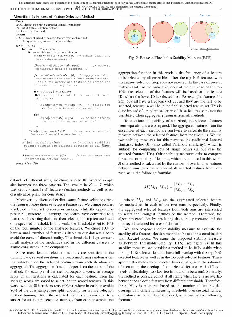
Fig. 2: Between Thresholds Stability Measure (BTS)
aggregation function in this work is the frequency of a featureto be selected by all ensembles. Then the top 10% features withthe highest selection frequency are selected. In the case of severalfeatures that had the same frequency at the end edge of the top10%, the selection of the features will be based on the featureID, where the lower ID is selected first. For example, features 14,255, 509 all have a frequency of 37, and they are the last to beselected, feature 14 will be in the final selected feature set. This isdone instead of a random selection of these features to reduce thevariability when aggregating features from all methods.
To calculate the stability of a method, the selected featuresfrom separate runs are compared. The aggregated features from theensembles of each method are run twice to calculate the stabilitymeasure between the selected features from the two runs. We usetwo stability measures for this purpose, the traditional Jaccardsimilarity index (JI) (also called Tanimoto similarity), which issuitable for comparing sets of single points (in our case theselected features’ IDs). Other stability measures exist to comparethe scores or ranking of features, which are not used in this work.JI of a method is calculated by the number of overlapping featuresbetween runs, over the number of all selected features from bothruns, as in the following formula:
JI(Mr1,Mr2) =|Mr1 ∩Mr2||Mr1 ∪Mr2|
where Mr1 and Mr2 are the aggregated selected featurefor method M in each of the two runs, respectively. Finally,the aggregated selected features from both runs are intersectedto select the strongest features of the method. Therefore, thealgorithm concludes by producing the stability measure and theintersected selected features of the runs.
We also propose another stability measure to evaluate thestability of a feature selection method to be used in a combinationwith Jaccard index. We name the proposed stability measureas Between Thresholds Stability (BTS) (see figure 2). In thisstability measure, we consider a method to be fully stable whenthe top 10% selected features have full overlap with the top 20%selected features as well as in the top 50% selected features. Thesespecific thresholds were selected heuristically, with the rationaleof measuring the overlap of top selected features with differentlevels of flexibility (too lax, too firm, and in between). Similarly,the method is considered not at all stable when there is no overlapbetween the selected features from different thresholds. Therefore,the stability is measured based on the number of features thatoverlaps with different increasing thresholds over the total numberof features in the smallest threshold, as shown in the followingformula:
Authorized licensed use limited to: Australian National University. Downloaded on January 27,2021 at 05:45:51 UTC from IEEE Xplore. Restrictions apply.
1949-3045 (c) 2020 IEEE. Personal use is permitted, but republication/redistribution requires IEEE permission. See http://www.ieee.org/publications_standards/publications/rights/index.html for moreinformation.
This article has been accepted for publication in a future issue of this journal, but has not been fully edited. Content may change prior to final publication. Citation information: DOI10.1109/TAFFC.2020.3035535, IEEE Transactions on Affective Computing
IEEE TRANSACTIONS ON AFFECTIVE COMPUTING, VOL. X, NO. X, JANUARY 2020 8
TABLE 2: Summary of Aggregation Levels
Aggregation DescriptionMethod-level Selects the final feature set that is robust to ran-
domness based on stability measures of each featureselection method.Gives an insight into the strongest features that dif-ferentiate depressed behaviour in each modality.
Modality-level Accumulates the strongest features from each modal-ity and the combined modalities using intersect(strict) and union (lenient).Captures both features that interact with other fea-tures within individual modality and between differ-ent modalities.Mainly meant for modelling depression detection, aswell as generalising the selected features on differentdepression datasets.
Dataset-level Finds a set of features that could generalise depres-sion modelling regardless of the dataset using relaxedintersection.
BTS(M) =|Mth=10 ∩Mth=20 ∩Mth=50|
|Mth=10|where M is the feature selection method, and th is the usedthreshold. This is performed over the intersected features fromthe two runs for each threshold level, where each threshold levelfollows Algorithm 1 process.
Moreover, to evaluate the performance of the feature selectedmethods they were also compared to a random guess method,where we follow the same process (ensembles and runs) for arandom feature selection. Stability measures were calculated inthe same way for the random method.
4.3 Aggregation Phase
The process as explained so far, is performed over each featureselection method to select the most promising features in a featurespace. This is executed on each modality individually (e.g. SB) andon the combined modalities (All-M). We performed the processover the full feature space from all modalities (All-M) to find thestrongest features and their interactions when all modalities arefused. However, this could result in selecting features mostly fromthe strongest modality without giving a balance to other modalitiesin selecting their strongest features. This could be avoided byapplying the feature selection framework on individual modalitiesas well. Furthermore, this will be beneficial for generalisationinvestigation, since not all modalities exist in all depressiondatasets (i.e. no SB for AVEC dataset procedure).
To select a final feature set for interpretation and modelling, weperform two-stage feature aggregations in each dataset. The firstaggregation stage is on the feature selection Method-level, whilethe second stage is on Modality-level as described below andsummarised in Table 2. For generalisation investigation, Dataset-level aggregation is performed to select the common features thatare selected from individual datasets.
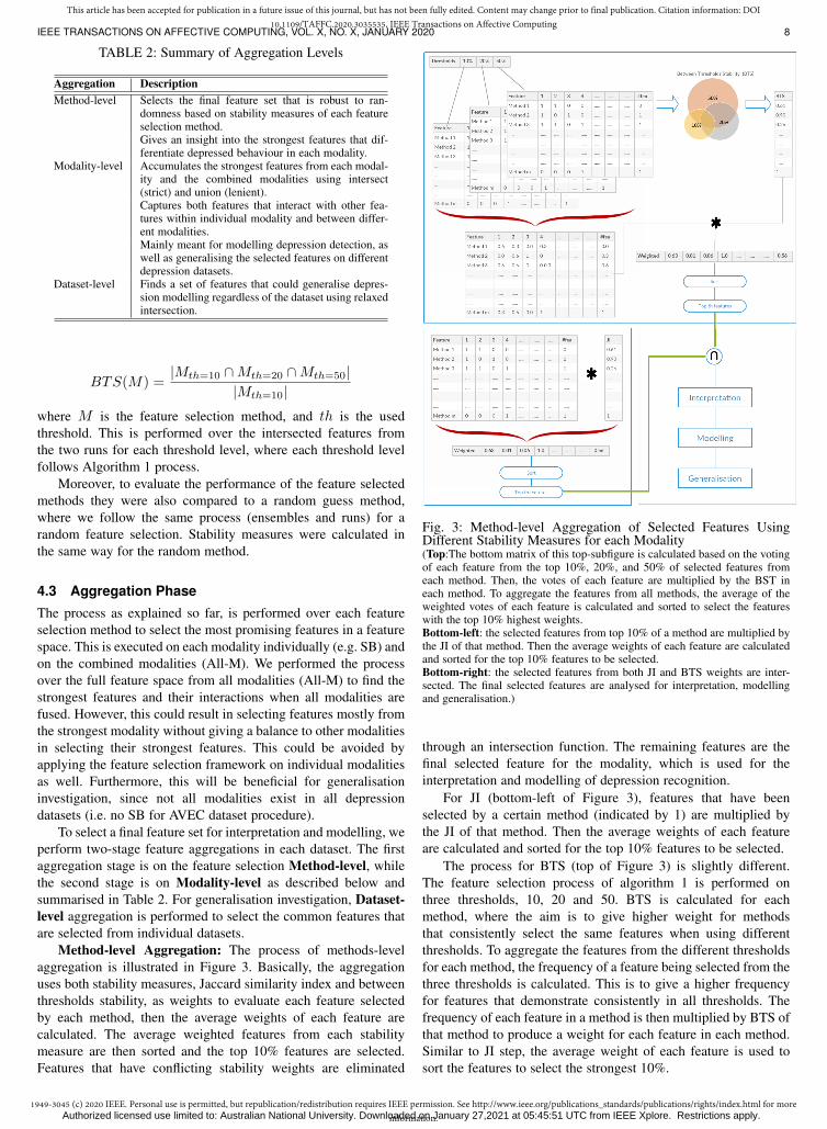
Method-level Aggregation: The process of methods-levelaggregation is illustrated in Figure 3. Basically, the aggregationuses both stability measures, Jaccard similarity index and betweenthresholds stability, as weights to evaluate each feature selectedby each method, then the average weights of each feature arecalculated. The average weighted features from each stabilitymeasure are then sorted and the top 10% features are selected.Features that have conflicting stability weights are eliminated
Fig. 3: Method-level Aggregation of Selected Features UsingDifferent Stability Measures for each Modality(Top:The bottom matrix of this top-subfigure is calculated based on the votingof each feature from the top 10%, 20%, and 50% of selected features fromeach method. Then, the votes of each feature are multiplied by the BST ineach method. To aggregate the features from all methods, the average of theweighted votes of each feature is calculated and sorted to select the featureswith the top 10% highest weights.Bottom-left: the selected features from top 10% of a method are multiplied bythe JI of that method. Then the average weights of each feature are calculatedand sorted for the top 10% features to be selected.Bottom-right: the selected features from both JI and BTS weights are inter-sected. The final selected features are analysed for interpretation, modellingand generalisation.)
through an intersection function. The remaining features are thefinal selected feature for the modality, which is used for theinterpretation and modelling of depression recognition.
For JI (bottom-left of Figure 3), features that have beenselected by a certain method (indicated by 1) are multiplied bythe JI of that method. Then the average weights of each featureare calculated and sorted for the top 10% features to be selected.
The process for BTS (top of Figure 3) is slightly different.The feature selection process of algorithm 1 is performed onthree thresholds, 10, 20 and 50. BTS is calculated for eachmethod, where the aim is to give higher weight for methodsthat consistently select the same features when using differentthresholds. To aggregate the features from the different thresholdsfor each method, the frequency of a feature being selected from thethree thresholds is calculated. This is to give a higher frequencyfor features that demonstrate consistently in all thresholds. Thefrequency of each feature in a method is then multiplied by BTS ofthat method to produce a weight for each feature in each method.Similar to JI step, the average weight of each feature is used tosort the features to select the strongest 10%.
Authorized licensed use limited to: Australian National University. Downloaded on January 27,2021 at 05:45:51 UTC from IEEE Xplore. Restrictions apply.
1949-3045 (c) 2020 IEEE. Personal use is permitted, but republication/redistribution requires IEEE permission. See http://www.ieee.org/publications_standards/publications/rights/index.html for moreinformation.
This article has been accepted for publication in a future issue of this journal, but has not been fully edited. Content may change prior to final publication. Citation information: DOI10.1109/TAFFC.2020.3035535, IEEE Transactions on Affective Computing
IEEE TRANSACTIONS ON AFFECTIVE COMPUTING, VOL. X, NO. X, JANUARY 2020 9
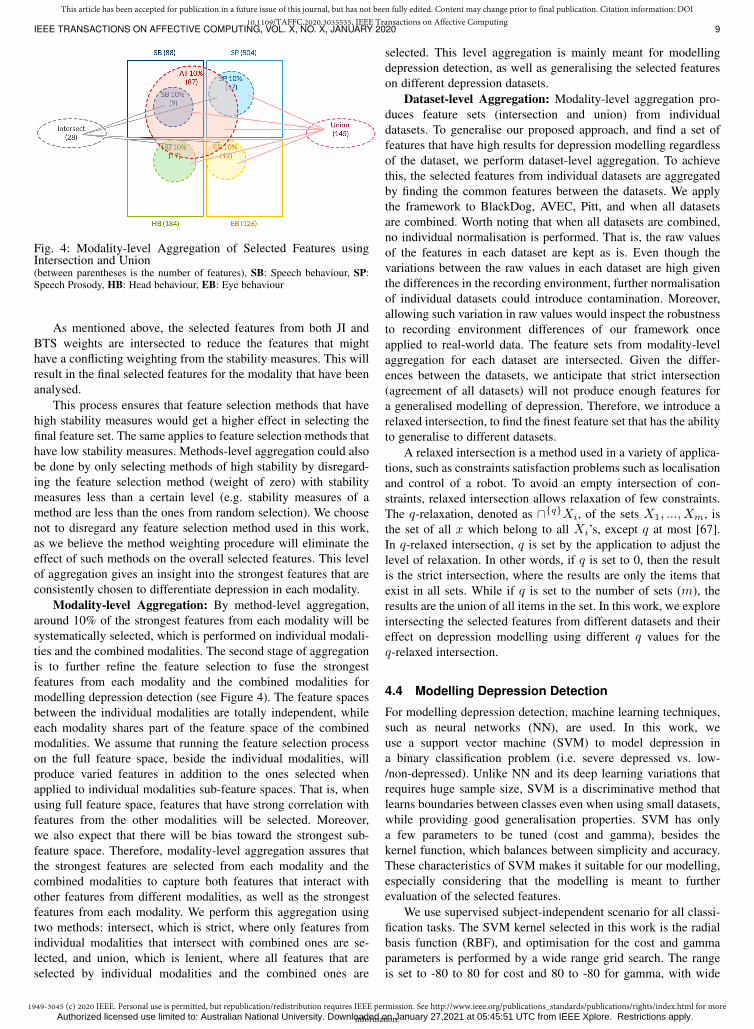
Fig. 4: Modality-level Aggregation of Selected Features usingIntersection and Union(between parentheses is the number of features), SB: Speech behaviour, SP:Speech Prosody, HB: Head behaviour, EB: Eye behaviour
As mentioned above, the selected features from both JI andBTS weights are intersected to reduce the features that mighthave a conflicting weighting from the stability measures. This willresult in the final selected features for the modality that have beenanalysed.
This process ensures that feature selection methods that havehigh stability measures would get a higher effect in selecting thefinal feature set. The same applies to feature selection methods thathave low stability measures. Methods-level aggregation could alsobe done by only selecting methods of high stability by disregard-ing the feature selection method (weight of zero) with stabilitymeasures less than a certain level (e.g. stability measures of amethod are less than the ones from random selection). We choosenot to disregard any feature selection method used in this work,as we believe the method weighting procedure will eliminate theeffect of such methods on the overall selected features. This levelof aggregation gives an insight into the strongest features that areconsistently chosen to differentiate depression in each modality.
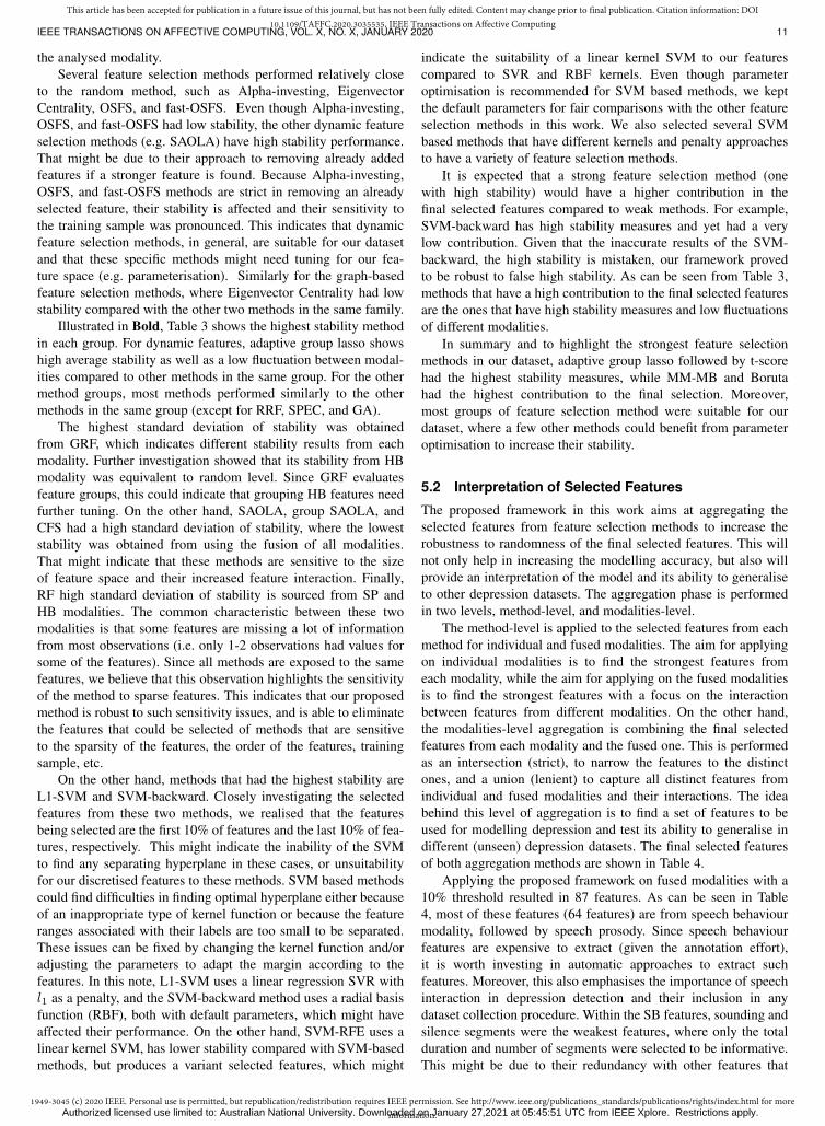
Modality-level Aggregation: By method-level aggregation,around 10% of the strongest features from each modality will besystematically selected, which is performed on individual modali-ties and the combined modalities. The second stage of aggregationis to further refine the feature selection to fuse the strongestfeatures from each modality and the combined modalities formodelling depression detection (see Figure 4). The feature spacesbetween the individual modalities are totally independent, whileeach modality shares part of the feature space of the combinedmodalities. We assume that running the feature selection processon the full feature space, beside the individual modalities, willproduce varied features in addition to the ones selected whenapplied to individual modalities sub-feature spaces. That is, whenusing full feature space, features that have strong correlation withfeatures from the other modalities will be selected. Moreover,we also expect that there will be bias toward the strongest sub-feature space. Therefore, modality-level aggregation assures thatthe strongest features are selected from each modality and thecombined modalities to capture both features that interact withother features from different modalities, as well as the strongestfeatures from each modality. We perform this aggregation usingtwo methods: intersect, which is strict, where only features fromindividual modalities that intersect with combined ones are se-lected, and union, which is lenient, where all features that areselected by individual modalities and the combined ones are
selected. This level aggregation is mainly meant for modellingdepression detection, as well as generalising the selected featureson different depression datasets.
Dataset-level Aggregation: Modality-level aggregation pro-duces feature sets (intersection and union) from individualdatasets. To generalise our proposed approach, and find a set offeatures that have high results for depression modelling regardlessof the dataset, we perform dataset-level aggregation. To achievethis, the selected features from individual datasets are aggregatedby finding the common features between the datasets. We applythe framework to BlackDog, AVEC, Pitt, and when all datasetsare combined. Worth noting that when all datasets are combined,no individual normalisation is performed. That is, the raw valuesof the features in each dataset are kept as is. Even though thevariations between the raw values in each dataset are high giventhe differences in the recording environment, further normalisationof individual datasets could introduce contamination. Moreover,allowing such variation in raw values would inspect the robustnessto recording environment differences of our framework onceapplied to real-world data. The feature sets from modality-levelaggregation for each dataset are intersected. Given the differ-ences between the datasets, we anticipate that strict intersection(agreement of all datasets) will not produce enough features fora generalised modelling of depression. Therefore, we introduce arelaxed intersection, to find the finest feature set that has the abilityto generalise to different datasets.
A relaxed intersection is a method used in a variety of applica-tions, such as constraints satisfaction problems such as localisationand control of a robot. To avoid an empty intersection of con-straints, relaxed intersection allows relaxation of few constraints.The q-relaxation, denoted as ∩{q}Xi, of the sets X1, ..., Xm, isthe set of all x which belong to all Xi’s, except q at most [67].In q-relaxed intersection, q is set by the application to adjust thelevel of relaxation. In other words, if q is set to 0, then the resultis the strict intersection, where the results are only the items thatexist in all sets. While if q is set to the number of sets (m), theresults are the union of all items in the set. In this work, we exploreintersecting the selected features from different datasets and theireffect on depression modelling using different q values for theq-relaxed intersection.
4.4 Modelling Depression Detection
For modelling depression detection, machine learning techniques,such as neural networks (NN), are used. In this work, weuse a support vector machine (SVM) to model depression ina binary classification problem (i.e. severe depressed vs. low-/non-depressed). Unlike NN and its deep learning variations thatrequires huge sample size, SVM is a discriminative method thatlearns boundaries between classes even when using small datasets,while providing good generalisation properties. SVM has onlya few parameters to be tuned (cost and gamma), besides thekernel function, which balances between simplicity and accuracy.These characteristics of SVM makes it suitable for our modelling,especially considering that the modelling is meant to furtherevaluation of the selected features.
We use supervised subject-independent scenario for all classi-fication tasks. The SVM kernel selected in this work is the radialbasis function (RBF), and optimisation for the cost and gammaparameters is performed by a wide range grid search. The rangeis set to -80 to 80 for cost and 80 to -80 for gamma, with wide
Authorized licensed use limited to: Australian National University. Downloaded on January 27,2021 at 05:45:51 UTC from IEEE Xplore. Restrictions apply.
1949-3045 (c) 2020 IEEE. Personal use is permitted, but republication/redistribution requires IEEE permission. See http://www.ieee.org/publications_standards/publications/rights/index.html for moreinformation.
This article has been accepted for publication in a future issue of this journal, but has not been fully edited. Content may change prior to final publication. Citation information: DOI10.1109/TAFFC.2020.3035535, IEEE Transactions on Affective Computing
IEEE TRANSACTIONS ON AFFECTIVE COMPUTING, VOL. X, NO. X, JANUARY 2020 10
to narrow search steps (40, 20, 10, 5, 2.5, and 0.5). For some setsof features, SVM was not able to find the optimal hyperplane,which might be because the range of these features and theirassociated labels are too small to be separated. We fixed this forthese sets by further adjusting the parameters search by increasingthe grid range and adding a fine 0.2 step (these instances aremarked with †). Leave-one-subject-out (LOSO) cross-validationwithout any overlap between training and testing data is used tomitigate for the relatively small number of observations in thedatasets. The performance of the modelling is measured in termsof average weighted (balanced) accuracy. For all modelling tasks,features were normalised by discretisation (converting continuesdata to discrete values). This is performed to be equivalent to thediscretisation step in the feature selection process and to minimisethe differences between the features in the three used datasets usedfor generalisation.
For comparisons, the depression recognition is modelled usingfull feature space for combined modalities and for sub-featurespaces for individual modalities, the final selected features fromcombined modalities and individual ones, and from random fea-ture selection method. These comparisons will highlight the effectof the selected features in modelling depression recognition.
4.5 Generalisation:To assess the validity of our proposed feature selection framework,and the robustness to randomness of the selected features indetecting depression, several generalisation approaches are per-formed. As an initial investigation, we generalise the results of themain depression dataset (BlackDog) on the other two datasets byevaluating the final selected features from the BlackDog dataset,by modelling depression severity detection using Pitt and AVECdepression datasets.
Then we generalise the framework and the selected featuremodelling through:
• Applying our proposed feature selection framework oneach dataset individually and as combined. This is toinvestigate the features that are commonly selected by alldatasets.
• Modelling depression detection using the selected featuresfrom each dataset and the combined datasets on each other.This is to evaluate the effectiveness of the selected featuresin modelling depression from unseen datasets.
• Performing dataset feature aggregation (Dataset-level) toexplore the ability to generalise the final selected featuresto the datasets. This is done through relaxation of intersec-tion.
5 APPLYING THE FRAMEWORK ON BLACKDOGDATASET
5.1 Feature Selection Methods ResultsDue to the sensitivity of feature selection methods to trainingsample, ensembles are used to increase the methods’ stability,where stability measures evaluate the sensitivity of a method. Inthis work, we used Jaccard index as a stability measure, sincethe output of all methods is in the form of a subset of features.We also proposed a new stability measure, which evaluates theselected features from different thresholds, we name it betweenthresholds stability. Feature selection methods were applied onindividual modalities (i.e. SB, SP, EB, HB) and their fusion.
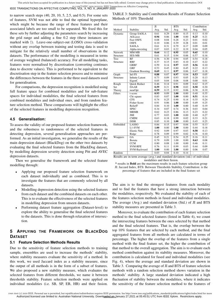
TABLE 3: Stability and Contribution Results of Feature SelectionMethods of 10% Threshold
JI BTS ContributionMethod Stability Avg. Std. Avg. Std. Avg. Std.Dynamic Group SAOLA 0.61 0.29 0.89 0.15 0.13 0.10
AGLasso 0.94 0.06 1.00 0.00 0.25 0.21Fast OSFS 0.08 0.04 0.28 0.23 0.01 0.02OSFS 0.10 0.06 0.39 0.28 0.01 0.01SAOLA 0.61 0.31 0.79 0.17 0.09 0.09Alpha-investing 0.07 0.03 0.22 0.19 0.04 0.05
Network MM-MB 0.64 0.12 0.95 0.05 0.65 0.10Structure SES-MB 0.61 0.15 0.94 0.06 0.57 0.16Tree RF 0.56 0.30 0.94 0.05 0.54 0.18Structure RRF 0.37 0.15 0.85 0.10 0.47 0.22
GRRF 0.59 0.14 0.97 0.05 0.56 0.10GRF 0.53 0.45 0.80 0.45 0.22 0.13Gradient Boosting 0.69 0.11 0.97 0.06 0.47 0.18
Graph Inf-FS 0.88 0.07 0.97 0.04 0.53 0.05Structure Infinite Latent 0.73 0.09 0.93 0.05 0.20 0.13
EigenC 0.05 0.04 0.06 0.08 0.00 0.01Rough Quick Reduct 0.46 0.14 0.91 0.09 0.42 0.15Set DAAR 0.59 0.21 0.98 0.02 0.50 0.20Theory nearOpt 0.59 0.15 0.92 0.06 0.38 0.19Filters t-score 0.93 0.09 1.00 0.00 0.40 0.35
Chi square 0.83 0.07 1.00 0.00 0.51 0.14CFS 0.74 0.25 0.90 0.14 0.35 0.24Fisher Score 0.91 0.06 1.00 0.00 0.49 0.25ReliefF 0.84 0.10 1.00 0.00 0.40 0.19SPEC 0.34 0.07 0.74 0.36 0.03 0.04MRMR 0.62 0.23 0.86 0.13 0.23 0.22JMI 0.77 0.03 1.00 0.00 0.40 0.27CMIM 0.63 0.18 0.99 0.02 0.33 0.21DISR 0.85 0.10 1.00 0.00 0.45 0.25
Embedded LASSO 0.84 0.15 0.97 0.04 0.55 0.13L1-SVM 1.00 0.00 1.00 0.00 0.44 0.18Elastic Nets 0.92 0.09 0.97 0.03 0.58 0.13Ridge 0.78 0.09 0.99 0.02 0.36 0.10
Wrappers GA 0.45 0.21 0.54 0.25 0.16 0.11Boruta 0.79 0.09 1.00 0.00 0.63 0.08CCM 0.80 0.08 1.00 0.00 0.46 0.11SVM-RFE 0.76 0.11 0.99 0.03 0.44 0.09SVM-Backward 1.00 0.00 1.00 0.00 0.06 0.07
Random 0.03 0.04 0.10 0.14 - -Results are in term average (avg.) and standard deviation (std.) of individual
modalities and their fusion.* results in Bold are the maximum results in each feature selection groupJI: Jaccard Index, BTS: Between Thresholds Stability, Contribution: is the
percentage of features that are included in the final feature set
The aim is to find the strongest features from each modalityand to find the features that have a strong interaction betweenthe modalities, respectively. We evaluated the stability of each ofthe features selection methods in fused and individual modalities.The average (Avg.) and standard deviation (Std.) of JI and BTSstability measures are presented in Table 3.
Moreover, to evaluate the contribution of each feature selectionmethod to the final selected features (listed in Table 4), we countthe intersecting features between the ones selected by that methodand the final selected features. That is, the overlap between thetop 10% features that are selected by each method, and the finalaggregated features from all methods are calculated in terms ofpercentage. The higher the overlap of the features from a singlemethod with the final feature set, the higher the contribution ofthat method to the overall aggregation. The aim is to evaluate eachmethod contribution against its stability measures. Moreover, thecontribution is calculated for fused and individual modalities (seeFig. 4), where the average and standard deviation are shown inTable 3. Comparing the average of JI and BTS of feature selectionmethods with a random selection method shows variation in themethods’ stability. A large standard deviation indicated a highfluctuation of stability between the modalities, where it indicatesthe sensitivity of the feature selection method to the features of
Authorized licensed use limited to: Australian National University. Downloaded on January 27,2021 at 05:45:51 UTC from IEEE Xplore. Restrictions apply.
1949-3045 (c) 2020 IEEE. Personal use is permitted, but republication/redistribution requires IEEE permission. See http://www.ieee.org/publications_standards/publications/rights/index.html for moreinformation.
This article has been accepted for publication in a future issue of this journal, but has not been fully edited. Content may change prior to final publication. Citation information: DOI10.1109/TAFFC.2020.3035535, IEEE Transactions on Affective Computing
IEEE TRANSACTIONS ON AFFECTIVE COMPUTING, VOL. X, NO. X, JANUARY 2020 11
the analysed modality.Several feature selection methods performed relatively close
to the random method, such as Alpha-investing, EigenvectorCentrality, OSFS, and fast-OSFS. Even though Alpha-investing,OSFS, and fast-OSFS had low stability, the other dynamic featureselection methods (e.g. SAOLA) have high stability performance.That might be due to their approach to removing already addedfeatures if a stronger feature is found. Because Alpha-investing,OSFS, and fast-OSFS methods are strict in removing an alreadyselected feature, their stability is affected and their sensitivity tothe training sample was pronounced. This indicates that dynamicfeature selection methods, in general, are suitable for our datasetand that these specific methods might need tuning for our fea-ture space (e.g. parameterisation). Similarly for the graph-basedfeature selection methods, where Eigenvector Centrality had lowstability compared with the other two methods in the same family.
Illustrated in Bold, Table 3 shows the highest stability methodin each group. For dynamic features, adaptive group lasso showshigh average stability as well as a low fluctuation between modal-ities compared to other methods in the same group. For the othermethod groups, most methods performed similarly to the othermethods in the same group (except for RRF, SPEC, and GA).
The highest standard deviation of stability was obtainedfrom GRF, which indicates different stability results from eachmodality. Further investigation showed that its stability from HBmodality was equivalent to random level. Since GRF evaluatesfeature groups, this could indicate that grouping HB features needfurther tuning. On the other hand, SAOLA, group SAOLA, andCFS had a high standard deviation of stability, where the loweststability was obtained from using the fusion of all modalities.That might indicate that these methods are sensitive to the sizeof feature space and their increased feature interaction. Finally,RF high standard deviation of stability is sourced from SP andHB modalities. The common characteristic between these twomodalities is that some features are missing a lot of informationfrom most observations (i.e. only 1-2 observations had values forsome of the features). Since all methods are exposed to the samefeatures, we believe that this observation highlights the sensitivityof the method to sparse features. This indicates that our proposedmethod is robust to such sensitivity issues, and is able to eliminatethe features that could be selected of methods that are sensitiveto the sparsity of the features, the order of the features, trainingsample, etc.
On the other hand, methods that had the highest stability areL1-SVM and SVM-backward. Closely investigating the selectedfeatures from these two methods, we realised that the featuresbeing selected are the first 10% of features and the last 10% of fea-tures, respectively. This might indicate the inability of the SVMto find any separating hyperplane in these cases, or unsuitabilityfor our discretised features to these methods. SVM based methodscould find difficulties in finding optimal hyperplane either becauseof an inappropriate type of kernel function or because the featureranges associated with their labels are too small to be separated.These issues can be fixed by changing the kernel function and/oradjusting the parameters to adapt the margin according to thefeatures. In this note, L1-SVM uses a linear regression SVR withl1 as a penalty, and the SVM-backward method uses a radial basisfunction (RBF), both with default parameters, which might haveaffected their performance. On the other hand, SVM-RFE uses alinear kernel SVM, has lower stability compared with SVM-basedmethods, but produces a variant selected features, which might
indicate the suitability of a linear kernel SVM to our featurescompared to SVR and RBF kernels. Even though parameteroptimisation is recommended for SVM based methods, we keptthe default parameters for fair comparisons with the other featureselection methods in this work. We also selected several SVMbased methods that have different kernels and penalty approachesto have a variety of feature selection methods.
It is expected that a strong feature selection method (onewith high stability) would have a higher contribution in thefinal selected features compared to weak methods. For example,SVM-backward has high stability measures and yet had a verylow contribution. Given that the inaccurate results of the SVM-backward, the high stability is mistaken, our framework provedto be robust to false high stability. As can be seen from Table 3,methods that have a high contribution to the final selected featuresare the ones that have high stability measures and low fluctuationsof different modalities.
In summary and to highlight the strongest feature selectionmethods in our dataset, adaptive group lasso followed by t-scorehad the highest stability measures, while MM-MB and Borutahad the highest contribution to the final selection. Moreover,most groups of feature selection method were suitable for ourdataset, where a few other methods could benefit from parameteroptimisation to increase their stability.
5.2 Interpretation of Selected Features
The proposed framework in this work aims at aggregating theselected features from feature selection methods to increase therobustness to randomness of the final selected features. This willnot only help in increasing the modelling accuracy, but also willprovide an interpretation of the model and its ability to generaliseto other depression datasets. The aggregation phase is performedin two levels, method-level, and modalities-level.
The method-level is applied to the selected features from eachmethod for individual and fused modalities. The aim for applyingon individual modalities is to find the strongest features fromeach modality, while the aim for applying on the fused modalitiesis to find the strongest features with a focus on the interactionbetween features from different modalities. On the other hand,the modalities-level aggregation is combining the final selectedfeatures from each modality and the fused one. This is performedas an intersection (strict), to narrow the features to the distinctones, and a union (lenient) to capture all distinct features fromindividual and fused modalities and their interactions. The ideabehind this level of aggregation is to find a set of features to beused for modelling depression and test its ability to generalise indifferent (unseen) depression datasets. The final selected featuresof both aggregation methods are shown in Table 4.
Applying the proposed framework on fused modalities with a10% threshold resulted in 87 features. As can be seen in Table4, most of these features (64 features) are from speech behaviourmodality, followed by speech prosody. Since speech behaviourfeatures are expensive to extract (given the annotation effort),it is worth investing in automatic approaches to extract suchfeatures. Moreover, this also emphasises the importance of speechinteraction in depression detection and their inclusion in anydataset collection procedure. Within the SB features, sounding andsilence segments were the weakest features, where only the totalduration and number of segments were selected to be informative.This might be due to their redundancy with other features that
Authorized licensed use limited to: Australian National University. Downloaded on January 27,2021 at 05:45:51 UTC from IEEE Xplore. Restrictions apply.
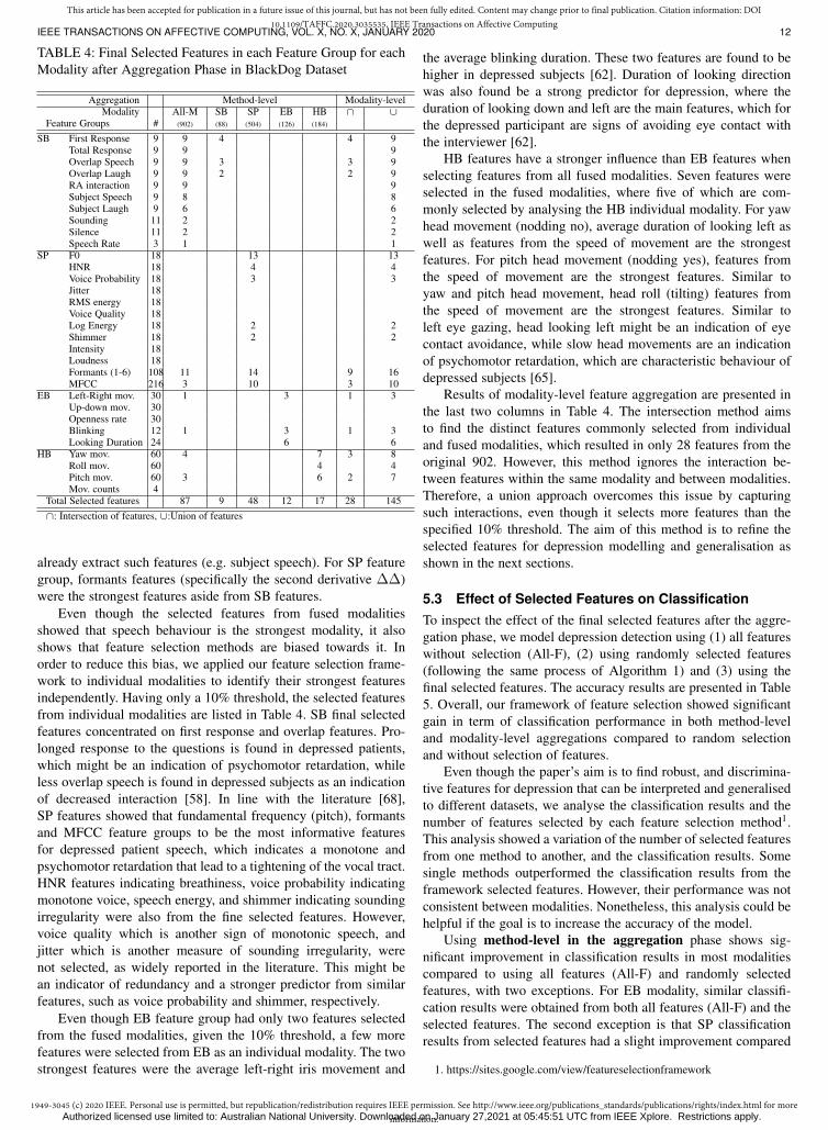
1949-3045 (c) 2020 IEEE. Personal use is permitted, but republication/redistribution requires IEEE permission. See http://www.ieee.org/publications_standards/publications/rights/index.html for moreinformation.
This article has been accepted for publication in a future issue of this journal, but has not been fully edited. Content may change prior to final publication. Citation information: DOI10.1109/TAFFC.2020.3035535, IEEE Transactions on Affective Computing
IEEE TRANSACTIONS ON AFFECTIVE COMPUTING, VOL. X, NO. X, JANUARY 2020 12
TABLE 4: Final Selected Features in each Feature Group for eachModality after Aggregation Phase in BlackDog Dataset
Aggregation Method-level Modality-levelModality All-M SB SP EB HB ∩ ∪
Feature Groups # (902) (88) (504) (126) (184)
SB First Response 9 9 4 4 9Total Response 9 9 9Overlap Speech 9 9 3 3 9Overlap Laugh 9 9 2 2 9RA interaction 9 9 9Subject Speech 9 8 8Subject Laugh 9 6 6Sounding 11 2 2Silence 11 2 2Speech Rate 3 1 1
SP F0 18 13 13HNR 18 4 4Voice Probability 18 3 3Jitter 18RMS energy 18Voice Quality 18Log Energy 18 2 2Shimmer 18 2 2Intensity 18Loudness 18Formants (1-6) 108 11 14 9 16MFCC 216 3 10 3 10
EB Left-Right mov. 30 1 3 1 3Up-down mov. 30Openness rate 30Blinking 12 1 3 1 3Looking Duration 24 6 6
HB Yaw mov. 60 4 7 3 8Roll mov. 60 4 4Pitch mov. 60 3 6 2 7Mov. counts 4
Total Selected features 87 9 48 12 17 28 145∩: Intersection of features, ∪:Union of features
already extract such features (e.g. subject speech). For SP featuregroup, formants features (specifically the second derivative ∆∆)were the strongest features aside from SB features.
Even though the selected features from fused modalitiesshowed that speech behaviour is the strongest modality, it alsoshows that feature selection methods are biased towards it. Inorder to reduce this bias, we applied our feature selection frame-work to individual modalities to identify their strongest featuresindependently. Having only a 10% threshold, the selected featuresfrom individual modalities are listed in Table 4. SB final selectedfeatures concentrated on first response and overlap features. Pro-longed response to the questions is found in depressed patients,which might be an indication of psychomotor retardation, whileless overlap speech is found in depressed subjects as an indicationof decreased interaction [58]. In line with the literature [68],SP features showed that fundamental frequency (pitch), formantsand MFCC feature groups to be the most informative featuresfor depressed patient speech, which indicates a monotone andpsychomotor retardation that lead to a tightening of the vocal tract.HNR features indicating breathiness, voice probability indicatingmonotone voice, speech energy, and shimmer indicating soundingirregularity were also from the fine selected features. However,voice quality which is another sign of monotonic speech, andjitter which is another measure of sounding irregularity, werenot selected, as widely reported in the literature. This might bean indicator of redundancy and a stronger predictor from similarfeatures, such as voice probability and shimmer, respectively.
Even though EB feature group had only two features selectedfrom the fused modalities, given the 10% threshold, a few morefeatures were selected from EB as an individual modality. The twostrongest features were the average left-right iris movement and
the average blinking duration. These two features are found to behigher in depressed subjects [62]. Duration of looking directionwas also found be a strong predictor for depression, where theduration of looking down and left are the main features, which forthe depressed participant are signs of avoiding eye contact withthe interviewer [62].
HB features have a stronger influence than EB features whenselecting features from all fused modalities. Seven features wereselected in the fused modalities, where five of which are com-monly selected by analysing the HB individual modality. For yawhead movement (nodding no), average duration of looking left aswell as features from the speed of movement are the strongestfeatures. For pitch head movement (nodding yes), features fromthe speed of movement are the strongest features. Similar toyaw and pitch head movement, head roll (tilting) features fromthe speed of movement are the strongest features. Similar toleft eye gazing, head looking left might be an indication of eyecontact avoidance, while slow head movements are an indicationof psychomotor retardation, which are characteristic behaviour ofdepressed subjects [65].
Results of modality-level feature aggregation are presented inthe last two columns in Table 4. The intersection method aimsto find the distinct features commonly selected from individualand fused modalities, which resulted in only 28 features from theoriginal 902. However, this method ignores the interaction be-tween features within the same modality and between modalities.Therefore, a union approach overcomes this issue by capturingsuch interactions, even though it selects more features than thespecified 10% threshold. The aim of this method is to refine theselected features for depression modelling and generalisation asshown in the next sections.
5.3 Effect of Selected Features on ClassificationTo inspect the effect of the final selected features after the aggre-gation phase, we model depression detection using (1) all featureswithout selection (All-F), (2) using randomly selected features(following the same process of Algorithm 1) and (3) using thefinal selected features. The accuracy results are presented in Table5. Overall, our framework of feature selection showed significantgain in term of classification performance in both method-leveland modality-level aggregations compared to random selectionand without selection of features.
Even though the paper’s aim is to find robust, and discrimina-tive features for depression that can be interpreted and generalisedto different datasets, we analyse the classification results and thenumber of features selected by each feature selection method1.This analysis showed a variation of the number of selected featuresfrom one method to another, and the classification results. Somesingle methods outperformed the classification results from theframework selected features. However, their performance was notconsistent between modalities. Nonetheless, this analysis could behelpful if the goal is to increase the accuracy of the model.
Using method-level in the aggregation phase shows sig-nificant improvement in classification results in most modalitiescompared to using all features (All-F) and randomly selectedfeatures, with two exceptions. For EB modality, similar classifi-cation results were obtained from both all features (All-F) and theselected features. The second exception is that SP classificationresults from selected features had a slight improvement compared
1. https://sites.google.com/view/featureselectionframework
Authorized licensed use limited to: Australian National University. Downloaded on January 27,2021 at 05:45:51 UTC from IEEE Xplore. Restrictions apply.
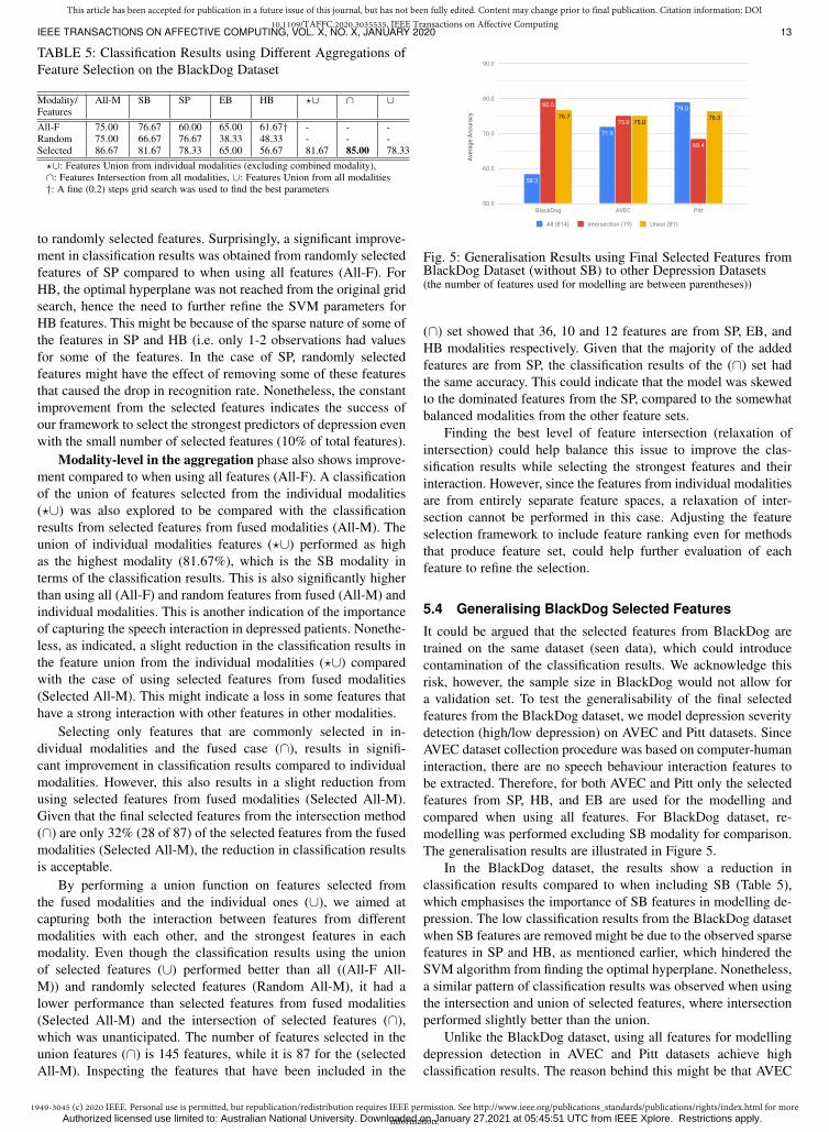
1949-3045 (c) 2020 IEEE. Personal use is permitted, but republication/redistribution requires IEEE permission. See http://www.ieee.org/publications_standards/publications/rights/index.html for moreinformation.
This article has been accepted for publication in a future issue of this journal, but has not been fully edited. Content may change prior to final publication. Citation information: DOI10.1109/TAFFC.2020.3035535, IEEE Transactions on Affective Computing
IEEE TRANSACTIONS ON AFFECTIVE COMPUTING, VOL. X, NO. X, JANUARY 2020 13
TABLE 5: Classification Results using Different Aggregations ofFeature Selection on the BlackDog Dataset
Modality/ All-M SB SP EB HB ?∪ ∩ ∪FeaturesAll-F 75.00 76.67 60.00 65.00 61.67† - - -Random 75.00 66.67 76.67 38.33 48.33 - - -Selected 86.67 81.67 78.33 65.00 56.67 81.67 85.00 78.33?∪: Features Union from individual modalities (excluding combined modality),∩: Features Intersection from all modalities, ∪: Features Union from all modalities†: A fine (0.2) steps grid search was used to find the best parameters
to randomly selected features. Surprisingly, a significant improve-ment in classification results was obtained from randomly selectedfeatures of SP compared to when using all features (All-F). ForHB, the optimal hyperplane was not reached from the original gridsearch, hence the need to further refine the SVM parameters forHB features. This might be because of the sparse nature of some ofthe features in SP and HB (i.e. only 1-2 observations had valuesfor some of the features. In the case of SP, randomly selectedfeatures might have the effect of removing some of these featuresthat caused the drop in recognition rate. Nonetheless, the constantimprovement from the selected features indicates the success ofour framework to select the strongest predictors of depression evenwith the small number of selected features (10% of total features).
Modality-level in the aggregation phase also shows improve-ment compared to when using all features (All-F). A classificationof the union of features selected from the individual modalities(?∪) was also explored to be compared with the classificationresults from selected features from fused modalities (All-M). Theunion of individual modalities features (?∪) performed as highas the highest modality (81.67%), which is the SB modality interms of the classification results. This is also significantly higherthan using all (All-F) and random features from fused (All-M) andindividual modalities. This is another indication of the importanceof capturing the speech interaction in depressed patients. Nonethe-less, as indicated, a slight reduction in the classification results inthe feature union from the individual modalities (?∪) comparedwith the case of using selected features from fused modalities(Selected All-M). This might indicate a loss in some features thathave a strong interaction with other features in other modalities.
Selecting only features that are commonly selected in in-dividual modalities and the fused case (∩), results in signifi-cant improvement in classification results compared to individualmodalities. However, this also results in a slight reduction fromusing selected features from fused modalities (Selected All-M).Given that the final selected features from the intersection method(∩) are only 32% (28 of 87) of the selected features from the fusedmodalities (Selected All-M), the reduction in classification resultsis acceptable.
By performing a union function on features selected fromthe fused modalities and the individual ones (∪), we aimed atcapturing both the interaction between features from differentmodalities with each other, and the strongest features in eachmodality. Even though the classification results using the unionof selected features (∪) performed better than all ((All-F All-M)) and randomly selected features (Random All-M), it had alower performance than selected features from fused modalities(Selected All-M) and the intersection of selected features (∩),which was unanticipated. The number of features selected in theunion features (∩) is 145 features, while it is 87 for the (selectedAll-M). Inspecting the features that have been included in the
58.3
71.9
79.080.0
75.0
68.4
76.775.0
76.3
Aver
age
Accu
racy
50.0
60.0
70.0
80.0
90.0
BlackDog AVEC Pitt
All (814) Intersection (19) Union (81)
Fig. 5: Generalisation Results using Final Selected Features fromBlackDog Dataset (without SB) to other Depression Datasets(the number of features used for modelling are between parentheses))
(∩) set showed that 36, 10 and 12 features are from SP, EB, andHB modalities respectively. Given that the majority of the addedfeatures are from SP, the classification results of the (∩) set hadthe same accuracy. This could indicate that the model was skewedto the dominated features from the SP, compared to the somewhatbalanced modalities from the other feature sets.
Finding the best level of feature intersection (relaxation ofintersection) could help balance this issue to improve the clas-sification results while selecting the strongest features and theirinteraction. However, since the features from individual modalitiesare from entirely separate feature spaces, a relaxation of inter-section cannot be performed in this case. Adjusting the featureselection framework to include feature ranking even for methodsthat produce feature set, could help further evaluation of eachfeature to refine the selection.
5.4 Generalising BlackDog Selected Features
It could be argued that the selected features from BlackDog aretrained on the same dataset (seen data), which could introducecontamination of the classification results. We acknowledge thisrisk, however, the sample size in BlackDog would not allow fora validation set. To test the generalisability of the final selectedfeatures from the BlackDog dataset, we model depression severitydetection (high/low depression) on AVEC and Pitt datasets. SinceAVEC dataset collection procedure was based on computer-humaninteraction, there are no speech behaviour interaction features tobe extracted. Therefore, for both AVEC and Pitt only the selectedfeatures from SP, HB, and EB are used for the modelling andcompared when using all features. For BlackDog dataset, re-modelling was performed excluding SB modality for comparison.The generalisation results are illustrated in Figure 5.
In the BlackDog dataset, the results show a reduction inclassification results compared to when including SB (Table 5),which emphasises the importance of SB features in modelling de-pression. The low classification results from the BlackDog datasetwhen SB features are removed might be due to the observed sparsefeatures in SP and HB, as mentioned earlier, which hindered theSVM algorithm from finding the optimal hyperplane. Nonetheless,a similar pattern of classification results was observed when usingthe intersection and union of selected features, where intersectionperformed slightly better than the union.
Unlike the BlackDog dataset, using all features for modellingdepression detection in AVEC and Pitt datasets achieve highclassification results. The reason behind this might be that AVEC
Authorized licensed use limited to: Australian National University. Downloaded on January 27,2021 at 05:45:51 UTC from IEEE Xplore. Restrictions apply.
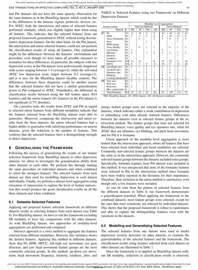
1949-3045 (c) 2020 IEEE. Personal use is permitted, but republication/redistribution requires IEEE permission. See http://www.ieee.org/publications_standards/publications/rights/index.html for moreinformation.
This article has been accepted for publication in a future issue of this journal, but has not been fully edited. Content may change prior to final publication. Citation information: DOI10.1109/TAFFC.2020.3035535, IEEE Transactions on Affective Computing
IEEE TRANSACTIONS ON AFFECTIVE COMPUTING, VOL. X, NO. X, JANUARY 2020 14
and Pitt datasets did not have the same sparsity observation forthe same features as in the BlackDog dataset, which could be dueto the differences in the datasets signals, protocols, devices, etc.For AVEC, both the intersection and union of selected featuresperformed similarly, which was slightly higher than when usingall features. This indicates that the selected features from ourproposed framework generalised to AVEC without losing discrim-inative depression features. On the other hand, for the Pitt dataset,the intersection and union selected features could not out-performthe classification results of using all features. One explanationmight be the differences between the datasets’ environment andprocedure, even though we have taken all possible measures tonormalise for these differences. In particular, the subjects with lowdepression scores in the Pitt dataset were professionally diagnosedwith scores ranging between 1-5 (average=2), while the self-ratedAVEC low depression score ranges between 0-2 (average=1),and it is zero for the BlackDog dataset (healthy control). Thedifferences between these diagnoses could be another reasonthat the selected features did not have a similar generalisationpower in Pitt compared to AVEC. Nonetheless, the difference inclassification results between using the full feature space (814features) and the union features (81 features) in the Pitt dataset isnot significant (2.7% absolute).
On a positive note, the results from AVEC and Pitt in regardto selected union features from different modalities indicate thatthe features selected from the BlackDog dataset were able togeneralise. Moreover, comparing the intersection and union re-sults from the three datasets, the union selected features had ahigher ability to generalise with satisfying performance on unseendatasets, given the reduction in the number of features. Thisconfirms that the selected features have a distinguishing strengthto detect depression.
6 GENERALISING THE FRAMEWORK
Following the success of generalising the results of our featureselection framework from BlackDog dataset to other depressiondatasets, we chose to investigate the generalisation ability fromother datasets to each other. We perform this through runningthe same procedure on individual datasets and when combinedto select the strongest features. The selected features from eachdataset are then used for modelling depression in each datasetindividually. Finally, we perform a dataset-level aggregation usingrelaxation of intersection to explore the level of feature intersec-tion that would produce the good classification results on all thethree datasets and when combined.
6.1 Datasets Selected FeaturesApplying our proposed feature selection framework on differentdatasets results in selecting features from each dataset (see Table6). For BlackDog dataset, we have re-run the framework excludingSB modality to have fair comparisons with the other datasets.As with BlackDog dataset, two approaches of modality-levelaggregations are performed and compared.
Intersect approach is a strict method to aggregate the featuresselected from different modalities. However, this strictness showsthe distinct features. Applying this method in different datasets,show that F0, HNR, MFCC, left-right eye movement, eye gazedirection, and yaw head movement feature groups are the mostcommonly selected groups. In this method, up-down eye move-ment, head movement frequency, intensity, loudness, jitter, and
TABLE 6: Selected Features using our Framework on DifferentDepression Datasets
Modality-Level AggregationFeature Group Intersect Methods Union Methods
Dataset # BD AV Pitt AD BD AV Pitt ADSP F0 18 11 16 2 5 16 18 10 15
HNR 18 3 1 4 4 6 10 14 6Voice Probability 18 2 3 3 9 5 5Jitter 18 1 1RMS energy 18Voice Quality 18 6 1 1 6 1 3Log Energy 18 1 2Shimmer 18 2 3 2 3 2 7 2Intensity 18 1Loudness 18Formants (1-6) 108 14 15 8 23 22 5 10MFCC 216 9 5 9 15 10 9 23 20
EB Left-Right mov. 30 2 1 3 3 3 1 5 3Up-down mov. 30 1 1 2 2 2Openness rate 30 5 2 1 2 6 2 1Blinking 12 3 1 1 5 1 2Looking Durations24 5 1 5 7 6 3 6 9
HB Yaw mov. 60 3 1 4 3 7 5 8 5Roll mov. 60 4 2 4 7 12 9Pitch mov. 60 2 2 3 6 5 7 5Mov. count totals 4 1 3Total #features 814 55 53 43 58 97 105 113 97
*BD: BlackDog dataset, AV: AVEC dataset, AD: All Datasets combined
energy feature groups were not selected in the majority of thedatasets, which indicates either a weak contribution in depressionor redundancy with other already selected features. Differencesbetween the datasets exist in selected feature groups in the in-tersection method. The feature groups that were not selected forBlackDog dataset, voice quality and eye openness rate, while forAVEC they are shimmer, eye blinking, and pitch head movement,and for Pitt it is formants.
Union approach of the modality-level aggregation is morelenient than the intersection approach, where all features that havebeen selected from individual and fused modalities are selected.Commonly non-selected feature groups between the datasets arethe same as in the intersection approach. However, the commonlyselected feature groups between the datasets included extra groups.Specifically, formants features from Pitt dataset were included inthis method. It was unexpected that none of the formants featureswere selected in Pitt in the intersection method since formantshave been widely reported in the literature for their importance.Therefore, their inclusion in the union method is satisfactory, eventhough only a few features were included.
As can be seen from the pattern of selected features fromthe different datasets in Table 6, our framework demonstratesa generalisation potential. When applying the framework to thecombined datasets, most feature groups were selected, except forthe ones that were commonly not selected by individual datasets.This shows that the proposed framework is robust to randomnessand able to capture the distinguishing features even with thevariations in the datasets.
6.2 Modelling and Generalising Selected Features
The selected features from one dataset were used to modeldepression severity detection on other datasets, to examine thegeneralisability of the selected features and the framework. Theclassification results using features selected from each dataset onother datasets are illustrated in Table 7.
Since the framework is re-applied on BlackDog dataset with-out SB modality, reduction in classification results is observed,
Authorized licensed use limited to: Australian National University. Downloaded on January 27,2021 at 05:45:51 UTC from IEEE Xplore. Restrictions apply.
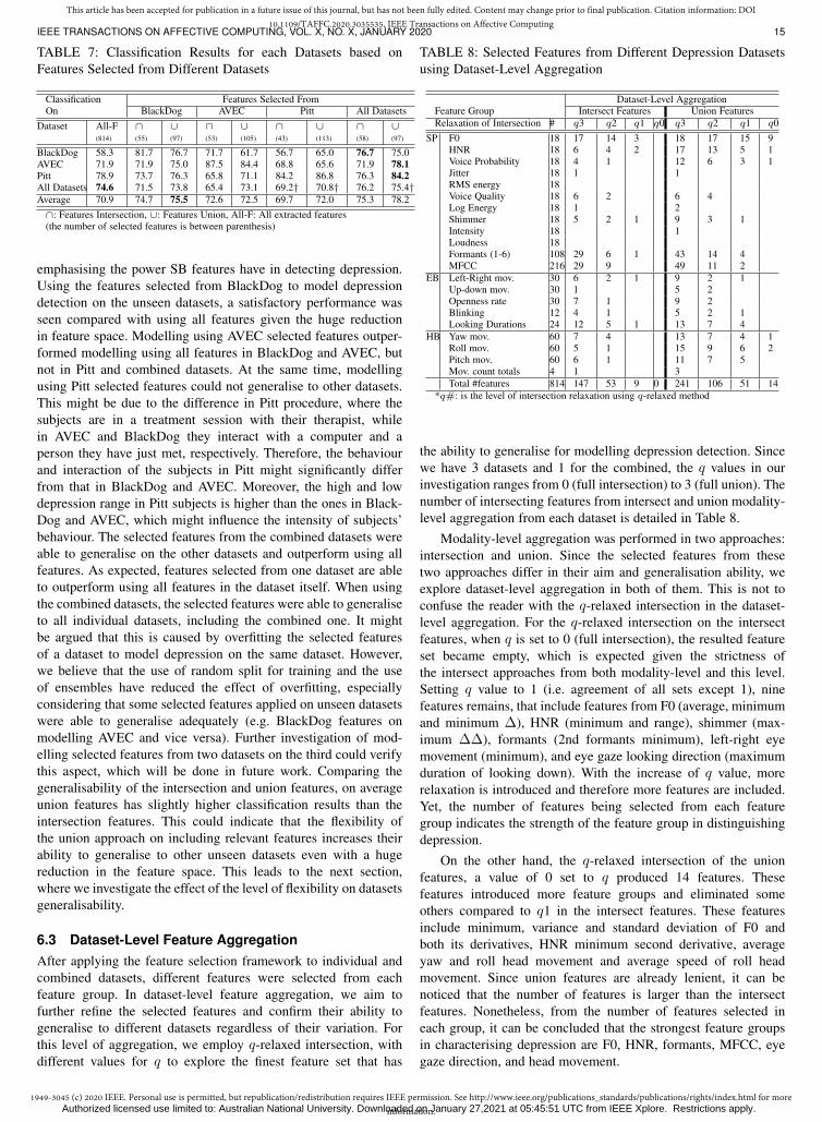
1949-3045 (c) 2020 IEEE. Personal use is permitted, but republication/redistribution requires IEEE permission. See http://www.ieee.org/publications_standards/publications/rights/index.html for moreinformation.
This article has been accepted for publication in a future issue of this journal, but has not been fully edited. Content may change prior to final publication. Citation information: DOI10.1109/TAFFC.2020.3035535, IEEE Transactions on Affective Computing
IEEE TRANSACTIONS ON AFFECTIVE COMPUTING, VOL. X, NO. X, JANUARY 2020 15
TABLE 7: Classification Results for each Datasets based onFeatures Selected from Different Datasets
Classification Features Selected FromOn BlackDog AVEC Pitt All Datasets
Dataset All-F ∩ ∪ ∩ ∪ ∩ ∪ ∩ ∪(814) (55) (97) (53) (105) (43) (113) (58) (97)
BlackDog 58.3 81.7 76.7 71.7 61.7 56.7 65.0 76.7 75.0AVEC 71.9 71.9 75.0 87.5 84.4 68.8 65.6 71.9 78.1Pitt 78.9 73.7 76.3 65.8 71.1 84.2 86.8 76.3 84.2All Datasets 74.6 71.5 73.8 65.4 73.1 69.2† 70.8† 76.2 75.4†Average 70.9 74.7 75.5 72.6 72.5 69.7 72.0 75.3 78.2∩: Features Intersection, ∪: Features Union, All-F: All extracted features(the number of selected features is between parenthesis)
emphasising the power SB features have in detecting depression.Using the features selected from BlackDog to model depressiondetection on the unseen datasets, a satisfactory performance wasseen compared with using all features given the huge reductionin feature space. Modelling using AVEC selected features outper-formed modelling using all features in BlackDog and AVEC, butnot in Pitt and combined datasets. At the same time, modellingusing Pitt selected features could not generalise to other datasets.This might be due to the difference in Pitt procedure, where thesubjects are in a treatment session with their therapist, whilein AVEC and BlackDog they interact with a computer and aperson they have just met, respectively. Therefore, the behaviourand interaction of the subjects in Pitt might significantly differfrom that in BlackDog and AVEC. Moreover, the high and lowdepression range in Pitt subjects is higher than the ones in Black-Dog and AVEC, which might influence the intensity of subjects’behaviour. The selected features from the combined datasets wereable to generalise on the other datasets and outperform using allfeatures. As expected, features selected from one dataset are ableto outperform using all features in the dataset itself. When usingthe combined datasets, the selected features were able to generaliseto all individual datasets, including the combined one. It mightbe argued that this is caused by overfitting the selected featuresof a dataset to model depression on the same dataset. However,we believe that the use of random split for training and the useof ensembles have reduced the effect of overfitting, especiallyconsidering that some selected features applied on unseen datasetswere able to generalise adequately (e.g. BlackDog features onmodelling AVEC and vice versa). Further investigation of mod-elling selected features from two datasets on the third could verifythis aspect, which will be done in future work. Comparing thegeneralisability of the intersection and union features, on averageunion features has slightly higher classification results than theintersection features. This could indicate that the flexibility ofthe union approach on including relevant features increases theirability to generalise to other unseen datasets even with a hugereduction in the feature space. This leads to the next section,where we investigate the effect of the level of flexibility on datasetsgeneralisability.
6.3 Dataset-Level Feature AggregationAfter applying the feature selection framework to individual andcombined datasets, different features were selected from eachfeature group. In dataset-level feature aggregation, we aim tofurther refine the selected features and confirm their ability togeneralise to different datasets regardless of their variation. Forthis level of aggregation, we employ q-relaxed intersection, withdifferent values for q to explore the finest feature set that has
TABLE 8: Selected Features from Different Depression Datasetsusing Dataset-Level Aggregation
Dataset-Level AggregationFeature Group Intersect Features Union FeaturesRelaxation of Intersection # q3 q2 q1 q0 q3 q2 q1 q0
SP F0 18 17 14 3 18 17 15 9HNR 18 6 4 2 17 13 5 1Voice Probability 18 4 1 12 6 3 1Jitter 18 1 1RMS energy 18Voice Quality 18 6 2 6 4Log Energy 18 1 2Shimmer 18 5 2 1 9 3 1Intensity 18 1Loudness 18Formants (1-6) 108 29 6 1 43 14 4MFCC 216 29 9 49 11 2
EB Left-Right mov. 30 6 2 1 9 2 1Up-down mov. 30 1 5 2Openness rate 30 7 1 9 2Blinking 12 4 1 5 2 1Looking Durations 24 12 5 1 13 7 4
HB Yaw mov. 60 7 4 13 7 4 1Roll mov. 60 5 1 15 9 6 2Pitch mov. 60 6 1 11 7 5Mov. count totals 4 1 3Total #features 814 147 53 9 0 241 106 51 14
*q#: is the level of intersection relaxation using q-relaxed method
the ability to generalise for modelling depression detection. Sincewe have 3 datasets and 1 for the combined, the q values in ourinvestigation ranges from 0 (full intersection) to 3 (full union). Thenumber of intersecting features from intersect and union modality-level aggregation from each dataset is detailed in Table 8.
Modality-level aggregation was performed in two approaches:intersection and union. Since the selected features from thesetwo approaches differ in their aim and generalisation ability, weexplore dataset-level aggregation in both of them. This is not toconfuse the reader with the q-relaxed intersection in the dataset-level aggregation. For the q-relaxed intersection on the intersectfeatures, when q is set to 0 (full intersection), the resulted featureset became empty, which is expected given the strictness ofthe intersect approaches from both modality-level and this level.Setting q value to 1 (i.e. agreement of all sets except 1), ninefeatures remains, that include features from F0 (average, minimumand minimum ∆), HNR (minimum and range), shimmer (max-imum ∆∆), formants (2nd formants minimum), left-right eyemovement (minimum), and eye gaze looking direction (maximumduration of looking down). With the increase of q value, morerelaxation is introduced and therefore more features are included.Yet, the number of features being selected from each featuregroup indicates the strength of the feature group in distinguishingdepression.
On the other hand, the q-relaxed intersection of the unionfeatures, a value of 0 set to q produced 14 features. Thesefeatures introduced more feature groups and eliminated someothers compared to q1 in the intersect features. These featuresinclude minimum, variance and standard deviation of F0 andboth its derivatives, HNR minimum second derivative, averageyaw and roll head movement and average speed of roll headmovement. Since union features are already lenient, it can benoticed that the number of features is larger than the intersectfeatures. Nonetheless, from the number of features selected ineach group, it can be concluded that the strongest feature groupsin characterising depression are F0, HNR, formants, MFCC, eyegaze direction, and head movement.
Authorized licensed use limited to: Australian National University. Downloaded on January 27,2021 at 05:45:51 UTC from IEEE Xplore. Restrictions apply.
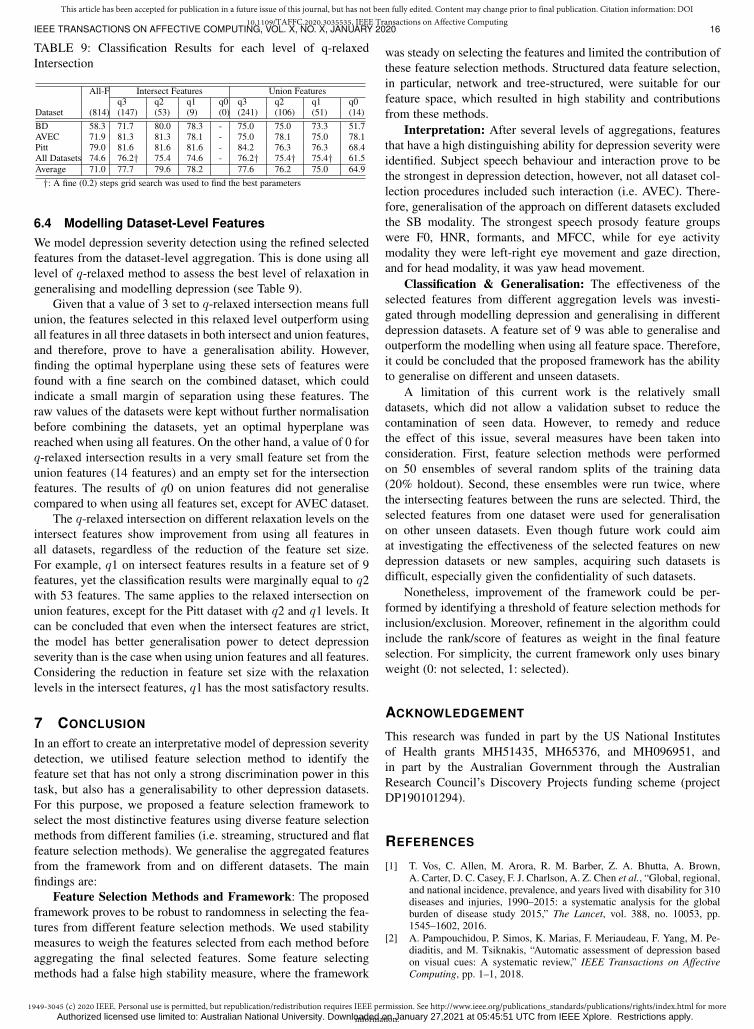
1949-3045 (c) 2020 IEEE. Personal use is permitted, but republication/redistribution requires IEEE permission. See http://www.ieee.org/publications_standards/publications/rights/index.html for moreinformation.
This article has been accepted for publication in a future issue of this journal, but has not been fully edited. Content may change prior to final publication. Citation information: DOI10.1109/TAFFC.2020.3035535, IEEE Transactions on Affective Computing
IEEE TRANSACTIONS ON AFFECTIVE COMPUTING, VOL. X, NO. X, JANUARY 2020 16
TABLE 9: Classification Results for each level of q-relaxedIntersection
All-F Intersect Features Union Featuresq3 q2 q1 q0 q3 q2 q1 q0
Dataset (814) (147) (53) (9) (0) (241) (106) (51) (14)BD 58.3 71.7 80.0 78.3 - 75.0 75.0 73.3 51.7AVEC 71.9 81.3 81.3 78.1 - 75.0 78.1 75.0 78.1Pitt 79.0 81.6 81.6 81.6 - 84.2 76.3 76.3 68.4All Datasets 74.6 76.2† 75.4 74.6 - 76.2† 75.4† 75.4† 61.5Average 71.0 77.7 79.6 78.2 77.6 76.2 75.0 64.9†: A fine (0.2) steps grid search was used to find the best parameters
6.4 Modelling Dataset-Level FeaturesWe model depression severity detection using the refined selectedfeatures from the dataset-level aggregation. This is done using alllevel of q-relaxed method to assess the best level of relaxation ingeneralising and modelling depression (see Table 9).
Given that a value of 3 set to q-relaxed intersection means fullunion, the features selected in this relaxed level outperform usingall features in all three datasets in both intersect and union features,and therefore, prove to have a generalisation ability. However,finding the optimal hyperplane using these sets of features werefound with a fine search on the combined dataset, which couldindicate a small margin of separation using these features. Theraw values of the datasets were kept without further normalisationbefore combining the datasets, yet an optimal hyperplane wasreached when using all features. On the other hand, a value of 0 forq-relaxed intersection results in a very small feature set from theunion features (14 features) and an empty set for the intersectionfeatures. The results of q0 on union features did not generalisecompared to when using all features set, except for AVEC dataset.
The q-relaxed intersection on different relaxation levels on theintersect features show improvement from using all features inall datasets, regardless of the reduction of the feature set size.For example, q1 on intersect features results in a feature set of 9features, yet the classification results were marginally equal to q2with 53 features. The same applies to the relaxed intersection onunion features, except for the Pitt dataset with q2 and q1 levels. Itcan be concluded that even when the intersect features are strict,the model has better generalisation power to detect depressionseverity than is the case when using union features and all features.Considering the reduction in feature set size with the relaxationlevels in the intersect features, q1 has the most satisfactory results.
7 CONCLUSION
In an effort to create an interpretative model of depression severitydetection, we utilised feature selection method to identify thefeature set that has not only a strong discrimination power in thistask, but also has a generalisability to other depression datasets.For this purpose, we proposed a feature selection framework toselect the most distinctive features using diverse feature selectionmethods from different families (i.e. streaming, structured and flatfeature selection methods). We generalise the aggregated featuresfrom the framework from and on different datasets. The mainfindings are:
Feature Selection Methods and Framework: The proposedframework proves to be robust to randomness in selecting the fea-tures from different feature selection methods. We used stabilitymeasures to weigh the features selected from each method beforeaggregating the final selected features. Some feature selectingmethods had a false high stability measure, where the framework
was steady on selecting the features and limited the contribution ofthese feature selection methods. Structured data feature selection,in particular, network and tree-structured, were suitable for ourfeature space, which resulted in high stability and contributionsfrom these methods.
Interpretation: After several levels of aggregations, featuresthat have a high distinguishing ability for depression severity wereidentified. Subject speech behaviour and interaction prove to bethe strongest in depression detection, however, not all dataset col-lection procedures included such interaction (i.e. AVEC). There-fore, generalisation of the approach on different datasets excludedthe SB modality. The strongest speech prosody feature groupswere F0, HNR, formants, and MFCC, while for eye activitymodality they were left-right eye movement and gaze direction,and for head modality, it was yaw head movement.
Classification & Generalisation: The effectiveness of theselected features from different aggregation levels was investi-gated through modelling depression and generalising in differentdepression datasets. A feature set of 9 was able to generalise andoutperform the modelling when using all feature space. Therefore,it could be concluded that the proposed framework has the abilityto generalise on different and unseen datasets.
A limitation of this current work is the relatively smalldatasets, which did not allow a validation subset to reduce thecontamination of seen data. However, to remedy and reducethe effect of this issue, several measures have been taken intoconsideration. First, feature selection methods were performedon 50 ensembles of several random splits of the training data(20% holdout). Second, these ensembles were run twice, wherethe intersecting features between the runs are selected. Third, theselected features from one dataset were used for generalisationon other unseen datasets. Even though future work could aimat investigating the effectiveness of the selected features on newdepression datasets or new samples, acquiring such datasets isdifficult, especially given the confidentiality of such datasets.
Nonetheless, improvement of the framework could be per-formed by identifying a threshold of feature selection methods forinclusion/exclusion. Moreover, refinement in the algorithm couldinclude the rank/score of features as weight in the final featureselection. For simplicity, the current framework only uses binaryweight (0: not selected, 1: selected).
ACKNOWLEDGEMENT
This research was funded in part by the US National Institutesof Health grants MH51435, MH65376, and MH096951, andin part by the Australian Government through the AustralianResearch Council’s Discovery Projects funding scheme (projectDP190101294).
REFERENCES
[1] T. Vos, C. Allen, M. Arora, R. M. Barber, Z. A. Bhutta, A. Brown,A. Carter, D. C. Casey, F. J. Charlson, A. Z. Chen et al., “Global, regional,and national incidence, prevalence, and years lived with disability for 310diseases and injuries, 1990–2015: a systematic analysis for the globalburden of disease study 2015,” The Lancet, vol. 388, no. 10053, pp.1545–1602, 2016.
[2] A. Pampouchidou, P. Simos, K. Marias, F. Meriaudeau, F. Yang, M. Pe-diaditis, and M. Tsiknakis, “Automatic assessment of depression basedon visual cues: A systematic review,” IEEE Transactions on AffectiveComputing, pp. 1–1, 2018.
Authorized licensed use limited to: Australian National University. Downloaded on January 27,2021 at 05:45:51 UTC from IEEE Xplore. Restrictions apply.
1949-3045 (c) 2020 IEEE. Personal use is permitted, but republication/redistribution requires IEEE permission. See http://www.ieee.org/publications_standards/publications/rights/index.html for moreinformation.
This article has been accepted for publication in a future issue of this journal, but has not been fully edited. Content may change prior to final publication. Citation information: DOI10.1109/TAFFC.2020.3035535, IEEE Transactions on Affective Computing
IEEE TRANSACTIONS ON AFFECTIVE COMPUTING, VOL. X, NO. X, JANUARY 2020 17
[3] N. Cummins, S. Scherer, J. Krajewski, S. Schnieder, J. Epps, and T. F.Quatieri, “A review of depression and suicide risk assessment usingspeech analysis,” Speech Communication, vol. 71, pp. 10 – 49, 2015.
[4] Y. Zhu, Y. Shang, Z. Shao, and G. Guo, “Automated depression diagnosisbased on deep networks to encode facial appearance and dynamics,”IEEE Transactions on Affective Computing, vol. 9, no. 4, pp. 578–584,Oct 2018.
[5] Y. Suhara, Y. Xu, and A. S. Pentland, “Deepmood: Forecasting depressedmood based on self-reported histories via recurrent neural networks,”in Proceedings of the 26th International Conference on World WideWeb, ser. WWW ’17. Republic and Canton of Geneva, Switzerland:International World Wide Web Conferences Steering Committee, 2017,pp. 715–724.
[6] T. Alhanai, M. Ghassemi, and J. Glass, “Detecting depression withaudio/text sequence modeling of interviews,” Proceedings of the AnnualConference of the International Speech Communication Association,INTERSPEECH, vol. 2018-September, pp. 1716–1720, 2018.
[7] M. A. H. M. S’adan, A. Pampouchidou, and F. Meriaudeau, “Deeplearning techniques for depression assessment,” in 2018 InternationalConference on Intelligent and Advanced System (ICIAS), Aug 2018, pp.1–5.
[8] L. He, D. Jiang, and H. Sahli, “Automatic depression analysis using dy-namic facial appearance descriptor and dirichlet process fisher encoding,”IEEE Transactions on Multimedia, pp. 1–1, 2018.
[9] L. Wen, X. Li, G. Guo, and Y. Zhu, “Automated depression diagnosisbased on facial dynamic analysis and sparse coding,” IEEE Transactionson Information Forensics and Security, vol. 10, no. 7, pp. 1432–1441,July 2015.
[10] A. Mendiratta, F. Scibelli, A. M. Esposito, V. Capuano, L. Likforman-Sulem, M. N. Maldonato, A. Vinciarelli, and A. Esposito, Automatic De-tection of Depressive States from Speech. Cham: Springer InternationalPublishing, 2018, pp. 301–314.
[11] L. He and C. Cao, “Automated depression analysis using convolu-tional neural networks from speech,” Journal of Biomedical Informatics,vol. 83, pp. 103 – 111, 2018.
[12] S. Song, L. Shen, and M. Valstar, “Human behaviour-based automaticdepression analysis using hand-crafted statistics and deep learned spectralfeatures,” in 2018 13th IEEE International Conference on AutomaticFace Gesture Recognition (FG 2018), May 2018, pp. 158–165.
[13] K. Anis, H. Zakia, D. Mohamed, and C. Jeffrey, “Detecting depressionseverity by interpretable representations of motion dynamics,” in 201813th IEEE International Conference on Automatic Face Gesture Recog-nition (FG 2018), May 2018, pp. 739–745.
[14] K. Yu, X. Wu, W. Ding, and J. Pei, “Towards scalable and accurate onlinefeature selection for big data,” in 2014 IEEE International Conference onData Mining, Dec 2014, pp. 660–669.
[15] ——, “Scalable and accurate online feature selection for big data,” ACMTrans. Knowl. Discov. Data, vol. 11, no. 2, pp. 16:1–16:39, Dec. 2016.
[16] X. Wu, K. Yu, H. Wang, and W. Ding, “Online streaming featureselection,” ICML 2010 - Proceedings, 27th International Conference onMachine Learning, pp. 1159–1166, 2010.
[17] X. Wu, K. Yu, W. Ding, H. Wang, and X. Zhu, “Online feature selectionwith streaming features,” IEEE Transactions on Pattern Analysis andMachine Intelligence, vol. 35, no. 5, pp. 1178–1192, 2013.
[18] J. Zhou, D. Foster, R. Stine, and L. Ungar, “Streamwise feature selec-tion,” Journal of Machine Learning Research, vol. 7, pp. 1861–1885,2006.
[19] I. Tsamardinos, L. E. Brown, and C. F. Aliferis, “The max-minhill-climbing bayesian network structure learning algorithm,” MachineLearning, vol. 65, no. 1, pp. 31–78, Oct 2006.
[20] C. F. Aliferis, A. Statnikov, I. Tsamardinos, S. Mani, and X. D. Kout-soukos, “Local causal and markov blanket induction for causal discoveryand feature selection for classification part i: Algorithms and empiricalevaluation,” J. Mach. Learn. Res., vol. 11, pp. 171–234, Mar. 2010.
[21] R. Diaz-Uriarte and S. Alvarez de Andres, “Variable selection fromrandom forests: application to gene expression data,” arXiv e-prints, pp.q–bio/0 503 025, Mar. 2005.
[22] H. Deng and G. Runger, “Feature selection via regularized trees,” in The2012 International Joint Conference on Neural Networks (IJCNN), June2012, pp. 1–8.
[23] ——, “Gene selection with guided regularized random forest,” PatternRecognition, vol. 46, no. 12, pp. 3483 – 3489, 2013.
[24] B. Gregorutti, B. Michel, and P. Saint-Pierre, “Grouped variable impor-tance with random forests and application to multiple functional dataanalysis,” Computational Statistics & Data Analysis, vol. 90, pp. 15 –35, 2015.
[25] Z. Xu, G. Huang, K. Q. Weinberger, and A. X. Zheng, “Gradientboosted feature selection,” in Proceedings of the 20th ACM SIGKDDInternational Conference on Knowledge Discovery and Data Mining,ser. KDD ’14. New York, NY, USA: ACM, 2014, pp. 522–531.
[26] G. Roffo, S. Melzi, and M. Cristani, “Infinite feature selection,” in 2015IEEE International Conference on Computer Vision (ICCV), Dec 2015,pp. 4202–4210.
[27] G. Roffo, S. Melzi, U. Castellani, and A. Vinciarelli, “Infinite latentfeature selection: A probabilistic latent graph-based ranking approach,”Proceedings of the IEEE International Conference on Computer Vision,vol. 2017-October, pp. 1407–1415, 2017.
[28] G. Roffo and S. Melzi, “Features selection via eigenvector centrality,”Proceedings of New Frontiers in Mining Complex Patterns (NFMCP2016)(Oct 2016), 2016.
[29] Q. Shen and A. Chouchoulas, “A modular approach to generating fuzzyrules with reduced attributes for the monitoring of complex systems,”Engineering Applications of Artificial Intelligence, vol. 13, no. 3, pp.263 – 278, 2000.
[30] A. Janusz and D. Slezak, “Random probes in computation and assess-ment of approximate reducts,” in Rough Sets and Intelligent SystemsParadigms, M. Kryszkiewicz, C. Cornelis, D. Ciucci, J. Medina-Moreno,H. Motoda, and Z. W. Ras, Eds. Cham: Springer International Publish-ing, 2014, pp. 53–64.
[31] S. Zhao, E. C. C. Tsang, and D. Chen, “The model of fuzzy variableprecision rough sets,” IEEE Transactions on Fuzzy Systems, vol. 17,no. 2, pp. 451–467, April 2009.
[32] J. C. Davis, Statistics and Data Analysis in Geology, 2nd ed. New York,NY, USA: John Wiley & Sons, Inc., 1990.
[33] H. Liu and R. Setiono, “Chi2: feature selection and discretization ofnumeric attributes,” Proceedings of the International Conference on Toolswith Artificial Intelligence, pp. 388–391, 1995.
[34] M. A. Hall and L. A. Smith, “Feature selection for machine learning:comparing a correlation-based filter approach to the wrapper.” in FLAIRSconference, vol. 1999, 1999, pp. 235–239.
[35] R. O. Duda, P. E. Hart, and D. G. Stork, Pattern Classification (2NdEdition). New York, NY, USA: Wiley-Interscience, 2000.
[36] M. Robnik-Sikonja and I. Kononenko, “Theoretical and empirical analy-sis of relieff and rrelieff,” Machine Learning, vol. 53, no. 1, pp. 23–69,Oct 2003.
[37] Z. Zhao and H. Liu, “Spectral feature selection for supervised and unsu-pervised learning,” in Proceedings of the 24th International Conferenceon Machine Learning, ser. ICML ’07. New York, NY, USA: ACM,2007, pp. 1151–1157.
[38] H. Peng, F. Long, and C. Ding, “Feature selection based on mu-tual information: Criteria of max-dependency, max-relevance, and min-redundancy,” IEEE Transactions on Pattern Analysis and Machine Intel-ligence, vol. 27, no. 8, pp. 1226–1238, 2005.
[39] H. H. Yang and J. Moody, “Data visualization and feature selection: Newalgorithms for nongaussian data,” in Advances in Neural InformationProcessing Systems, 2000, pp. 687–693.
[40] F. Fleuret, “Fast binary feature selection with conditional mutual infor-mation,” Journal of Machine Learning Research, vol. 5, pp. 1531–1555,2004.
[41] P. Meyer, C. Schretter, and G. Bontempi, “Information-theoretic featureselection in microarray data using variable complementarity,” IEEEJournal on Selected Topics in Signal Processing, vol. 2, no. 3, pp. 261–274, 2008.
[42] R. Tibshirani, “The lasso method for variable selection in the cox model,”Statistics in medicine, vol. 16, no. 4, pp. 385–395, 1997.
[43] M. Y. Park and T. Hastie, “L1-regularization path algorithm for gener-alized linear models,” Journal of the Royal Statistical Society: Series B(Statistical Methodology), vol. 69, no. 4, pp. 659–677, 2007.
[44] H. Zou and T. Hastie, “Regularization and variable selection via theelastic net,” Journal of the Royal Statistical Society: Series B (StatisticalMethodology), vol. 67, no. 2, pp. 301–320, 2005.
[45] W. J. Fu, “Penalized regressions: The bridge versus the lasso,” Journalof Computational and Graphical Statistics, vol. 7, no. 3, pp. 397–416,1998.
[46] J. Yang and V. Honavar, Feature Subset Selection Using a GeneticAlgorithm. Boston, MA: Springer US, 1998, pp. 117–136.
[47] M. Kursa and W. Rudnicki, “Feature selection with the boruta package,”Journal of Statistical Software, vol. 36, no. 11, pp. 1–13, 2010.
[48] J. Chen, M. Stern, M. J. Wainwright, and M. I. Jordan, “Kernel feature se-lection via conditional covariance minimization,” in Advances in NeuralInformation Processing Systems 30, I. Guyon, U. V. Luxburg, S. Bengio,H. Wallach, R. Fergus, S. Vishwanathan, and R. Garnett, Eds. CurranAssociates, Inc., 2017, pp. 6949–6958.
Authorized licensed use limited to: Australian National University. Downloaded on January 27,2021 at 05:45:51 UTC from IEEE Xplore. Restrictions apply.
1949-3045 (c) 2020 IEEE. Personal use is permitted, but republication/redistribution requires IEEE permission. See http://www.ieee.org/publications_standards/publications/rights/index.html for moreinformation.
This article has been accepted for publication in a future issue of this journal, but has not been fully edited. Content may change prior to final publication. Citation information: DOI10.1109/TAFFC.2020.3035535, IEEE Transactions on Affective Computing
IEEE TRANSACTIONS ON AFFECTIVE COMPUTING, VOL. X, NO. X, JANUARY 2020 18
[49] I. Guyon, J. Weston, S. Barnhill, and V. Vapnik, “Gene selection forcancer classification using support vector machines,” Machine Learning,vol. 46, no. 1, pp. 389–422, Jan 2002.
[50] A. Rakotomamonjy, “Variable selection using svm-based criteria,” Jour-nal of Machine Learning Research, vol. 3, pp. 1357–1370, 2003.
[51] S. Alghowinem, R. Goecke, M. Wagner, J. Epps, M. Hyett, G. Parker,and M. Breakspear, “Multimodal depression detection: Fusion analysisof paralinguistic, head pose and eye gaze behaviors,” IEEE Transactionson Affective Computing, vol. 9, no. 4, pp. 478–490, Oct 2018.
[52] Y. Yang, C. Fairbairn, and J. F. Cohn, “Detecting depression severityfrom vocal prosody,” IEEE Transactions on Affective Computing, vol. 4,no. 2, pp. 142–150, April 2013.
[53] M. Valstar, B. Schuller, K. Smith, F. Eyben, B. Jiang, S. Bilakhia,S. Schnieder, R. Cowie, and M. Pantic, “Avec 2013: The continuousaudio/visual emotion and depression recognition challenge,” in Proceed-ings of the 3rd ACM International Workshop on Audio/Visual EmotionChallenge, ser. AVEC ’13. New York, NY, USA: ACM, 2013, pp.3–10.
[54] A. J. Rush, M. H. Trivedi, H. M. Ibrahim, T. J. Carmody, B. Arnow, D. N.Klein, J. C. Markowitz, P. T. Ninan, S. Kornstein, R. Manber et al., “The16-item quick inventory of depressive symptomatology (qids), clinicianrating (qids-c), and self-report (qids-sr): a psychometric evaluation inpatients with chronic major depression,” Biological psychiatry, vol. 54,no. 5, pp. 573–583, 2003.
[55] J. C. Fournier, R. J. DeRubeis, S. D. Hollon, S. Dimidjian, J. D.Amsterdam, R. C. Shelton, and J. Fawcett, “Antidepressant drug effectsand depression severity,” JAMA: The Journal of the American MedicalAssociation, vol. 303, no. 1, pp. 47–53, 2010.
[56] A. T. Beck, R. A. Steer, R. Ball, and W. Ranieri, “Comparison of BeckDepression Inventories -IA and -II in psychiatric outpatients,” Journal ofpersonality assessment, vol. 67, no. 3, pp. 588–597, Dec 1996.
[57] Depression Scores Conversion. (Online) Inventory of Depressive Symp-tomatology (IDS) and Quick Inventory of Depressive Symptomatology(QIDS).
[58] S. Alghowinem, R. Goecke, M. Wagner, J. Epps, M. Breakspear, andG. Parker, “From joyous to clinically depressed: Mood detection usingspontaneous speech,” Proceedings of the 25th International FloridaArtificial Intelligence Research Society Conference, FLAIRS-25, pp. 141–146, 2012.
[59] E. A. Stepanov, S. Lathuiliere, S. A. Chowdhury, A. Ghosh, R. Vieriu,N. Sebe, and G. Riccardi, “Depression severity estimation from multiplemodalities,” in 2018 IEEE 20th International Conference on e-HealthNetworking, Applications and Services (Healthcom), Sep. 2018, pp. 1–6.
[60] S. Alghowinem, R. Goecke, J. Epps, M. Wagner, and J. Cohn, “Cross-cultural depression recognition from vocal biomarkers,” Proceedingsof the Annual Conference of the International Speech CommunicationAssociation, INTERSPEECH, vol. 08-12-September-2016, pp. 1943–1947, 2016.
[61] N. Carvalho, E. Laurent, N. Noiret, G. Chopard, E. Haffen, D. Bennabi,and P. Vandel, “Eye movement in unipolar and bipolar depression: Asystematic review of the literature,” Frontiers in Psychology, vol. 6, p.1809, 2015.
[62] S. Alghowinem, R. Goecke, M. Wagner, G. Parker, and M. Breakspear,“Eye movement analysis for depression detection,” in 2013 IEEE Inter-national Conference on Image Processing, Sep. 2013, pp. 4220–4224.
[63] S. Alghowinem, R. Goecke, J. Cohn, M. Wagner, G. Parker, andM. Breakspear, “Cross-cultural detection of depression from nonverbalbehaviour,” 2015 11th IEEE International Conference and Workshops onAutomatic Face and Gesture Recognition, FG 2015, 2015.
[64] J. T. Fiquer, R. A. Moreno, J. Z. Canales, A. Cavalcanti, and C. Goren-stein, “Is nonverbal behavior in patients and interviewers relevant tothe assessment of depression and its recovery? a study with dutch andbrazilian patients,” Psychiatry Research, vol. 250, pp. 59 – 64, 2017.
[65] S. Alghowinem, R. Goecke, M. Wagner, G. Parkerx, and M. Breakspear,“Head pose and movement analysis as an indicator of depression,”in 2013 Humaine Association Conference on Affective Computing andIntelligent Interaction, Sep. 2013, pp. 283–288.
[66] H. Wang and C. Leng, “A note on adaptive group lasso,” ComputationalStatistics & Data Analysis, vol. 52, no. 12, pp. 5277 – 5286, 2008.
[67] L. Jaulin, “Robust set-membership state estimation; application to under-water robotics,” Automatica, vol. 45, no. 1, pp. 202 – 206, 2009.
[68] S. Alghowinem, R. Goecke, M. Wagner, J. Epps, G. Parker, andM. Breakspear, “Characterising depressed speech for classification,”Proceedings of the Annual Conference of the International SpeechCommunication Association, INTERSPEECH, pp. 2534–2538, 2013.
Sharifa Alghowinem currently holds a postdoctoralfellow position at Massachusetts Institute of Technol-ogy. She worked as a lecturer at University of Can-berra in 2011, research associate at Australian Na-tional University and hold a research and teachingposition at Prince Sultan University. She received herPhD at the Australian National University, ComputerScience Research School in 2015. She received herMSc in Software Engineering at University of Canberrain 2010, and her BSc in Computer Applications at KingSaud University in 2004. Her research interests include
speech processing, computer vision, affective computing, and machine learning.
Tom Gedeon received the BSc (Hons) and PhDdegrees from the University of Western Australia. Heis currently chair professor of Computer Science atthe Australian National University, Canberra, Australia,and leads the Human-Centred Computing Group at theResearch School of Computer Science. His researchinterests are in bio-inspired computing and in humancentred computing. He is a former president of theAsia-Pacific Neural Network Assembly and a formerPresident of the Computing Research and
Roland Goecke Roland Goecke is Professor of Af-fective Computing, Head of the Vision and SensingGroup, and Director of the Human-Centred Technol-ogy Research Centre at the University of Canberra.He received his Masters degree in Computer Sciencefrom the University of Rostock, Germany, in 1998 andhis Ph.D. in Computer Science from the Australian Na-tional University, Canberra, Australia, in 2004. Beforejoining the University of Canberra in 2008, he workedfor Seeing Machines, National ICT Australia and theFraunhofer Institute for Computer Graphics, Germany.
His research interests are in affective computing, pattern recognition, computervision, human-computer interaction and multimodal signal processing.
Jeffrey F. Cohn is a professor of psychology andpsychiatry at the University of Pittsburgh and an ad-junct professor at the Robotics Institute, Carnegie Mel-lon University. He has led interdisciplinary and inter-institutional efforts to develop advanced methods ofautomatic analysis and synthesis of facial and vocal ex-pression and applied them to research in human emo-tion,interpersonal processes, social development,andpsychopathology. He co-chaired the IEEE InternationalConference on Automatic Face and Gesture Recogni-tion (FG2015 and FG2008), the International Confer-
ence on Multimodal Interfaces in 2014 (ICMI2014), and the International Confer-ence on Affective Computing and Intelligent Interaction(ACII2009). His researchis supported in part by the US National Institutes of Health and the US NationalScience Foundation. He is an associate member of the IEEE.
Gordon Parker is Scientia Professor of Psychiatryat the University of New South Wales, and for 10 yearsheld the position of inaugural Executive Director of theBlack Dog Institute in Sydney, Australia. For nearly twodecades he was Head of the School of Psychiatry atUNSW and Director of Psychiatry at Prince of Walesand Prince Henry Hospitals. He is internationally recog-nised for his research into the causes and phenomenol-ogy of depressive and bipolar (mood) disorders. Suchresearch has been pivotal in challenging existing diag-nostic approaches, and has contributed to optimising
treatments across differing conditions. He received a Citation Laureate award inthe field of Psychology/Psychiatry in 2004. In 2007, Parker was elected as a Fellowof the Academy of the Social Sciences in Australia, and in 2010 was recipient ofan Officer of Order of Australia Award for distinguished service to psychiatry.
Authorized licensed use limited to: Australian National University. Downloaded on January 27,2021 at 05:45:51 UTC from IEEE Xplore. Restrictions apply.