Embed Size (px)
Citation preview

| 1CITS2401 Computer Analysis & Visualisation
Interpolation and curve
fitting
Lecture 9
CITS2401
Computer Analysis and Visualization
School of Computer Science and Software Engineering

| 2CITS2401 Computer Analysis & Visualisation
Summary
Interpolation
Curve fitting
Linear regression (for single variables)
Polynomial regression
Multiple variable regression
Non-linear terms in regression
| 3CITS2401 Computer Analysis & Visualisation
Interpolation
Suppose you have some known data points, and you wish to predict what other data points might be – how can you do this?
For example:
If at t = 1 second, distance traveled = 2m, and
at t = 5 seconds, distance traveled = 10m ...
What would be the distance traveled at, say, t = 3 seconds?
| 4CITS2401 Computer Analysis & Visualisation
Linear interpolation
The simplest interpolation technique is linear interpolation:
it assumes that data follows a straight line between adjacent measurements.
| 5CITS2401 Computer Analysis & Visualisation
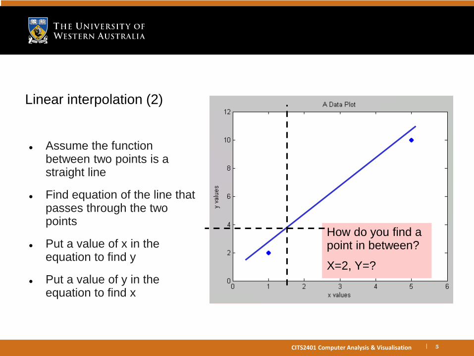
Linear interpolation (2)
Assume the function between two points is a straight line
Find equation of the line that passes through the two points
Put a value of x in the equation to find y
Put a value of y in the equation to find x
How do you find a point in between?
X=2, Y=?
| 6CITS2401 Computer Analysis & Visualisation
Linear interpolation in python
numpy.interp(x, xp, yp):
xp and yp give the x and y coordinates of the data points we have
x contains the x coordinates that we want interpolated y-values for.
| 7CITS2401 Computer Analysis & Visualisation
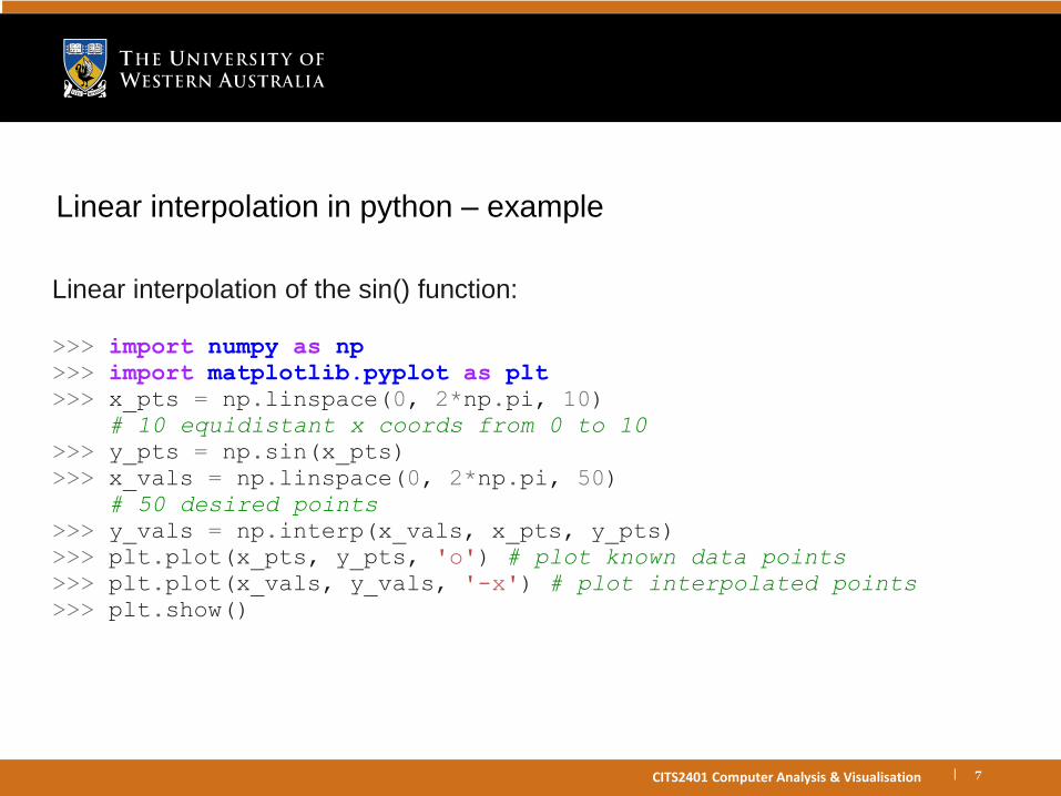
Linear interpolation in python – example
Linear interpolation of the sin() function:
>>> import numpy as np
>>> import matplotlib.pyplot as plt
>>> x_pts = np.linspace(0, 2*np.pi, 10)
# 10 equidistant x coords from 0 to 10
>>> y_pts = np.sin(x_pts)
>>> x_vals = np.linspace(0, 2*np.pi, 50)
# 50 desired points
>>> y_vals = np.interp(x_vals, x_pts, y_pts)
>>> plt.plot(x_pts, y_pts, 'o') # plot known data points
>>> plt.plot(x_vals, y_vals, '-x') # plot interpolated points
>>> plt.show()

| 8CITS2401 Computer Analysis & Visualisation
Linear interpolation in python – example (2)
| 9CITS2401 Computer Analysis & Visualisation
Cubic spline interpolation
Just as a linear interpolation is made up of linear segments – a cubic spline interpolation is made of segments of cubic polynomials, whose gradients match up at the measured data points.
These cubic polynomials are continuous up to their 2nd derivative.

| 10CITS2401 Computer Analysis & Visualisation
Cubic spline interpolation (2)
Using numpy and scipy, interpolation is done in 2 steps:
scipy.interpolate.splrep(x_pts, y_pts) – returns a tuple
representing the spline formulas needed
scipy.interpolate.splev(x_vals, splines) ("spline evaluate") – evaluate the spline data returned by splrep, and use it to estimate y
values.
| 11CITS2401 Computer Analysis & Visualisation
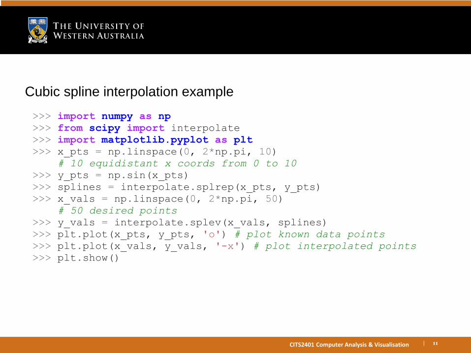
Cubic spline interpolation example
>>> import numpy as np
>>> from scipy import interpolate
>>> import matplotlib.pyplot as plt
>>> x_pts = np.linspace(0, 2*np.pi, 10)
# 10 equidistant x coords from 0 to 10
>>> y_pts = np.sin(x_pts)
>>> splines = interpolate.splrep(x_pts, y_pts)
>>> x_vals = np.linspace(0, 2*np.pi, 50)
# 50 desired points
>>> y_vals = interpolate.splev(x_vals, splines)
>>> plt.plot(x_pts, y_pts, 'o') # plot known data points
>>> plt.plot(x_vals, y_vals, '-x') # plot interpolated points
>>> plt.show()
| 12CITS2401 Computer Analysis & Visualisation
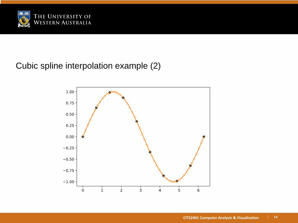
Cubic spline interpolation example (2)

| 13CITS2401 Computer Analysis & Visualisation
2D interpolation
Just as we can do linear interpolation to estimate y values given x values –i.e. estimating a one-variable function f(x) – we can also do linear interpolation of a two-variable function f(x,y).
| 14CITS2401 Computer Analysis & Visualisation
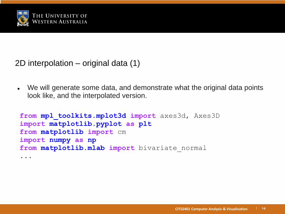
2D interpolation – original data (1)
We will generate some data, and demonstrate what the original data points look like, and the interpolated version.
from mpl_toolkits.mplot3d import axes3d, Axes3D
import matplotlib.pyplot as plt
from matplotlib import cm
import numpy as np
from matplotlib.mlab import bivariate_normal
...
| 15CITS2401 Computer Analysis & Visualisation
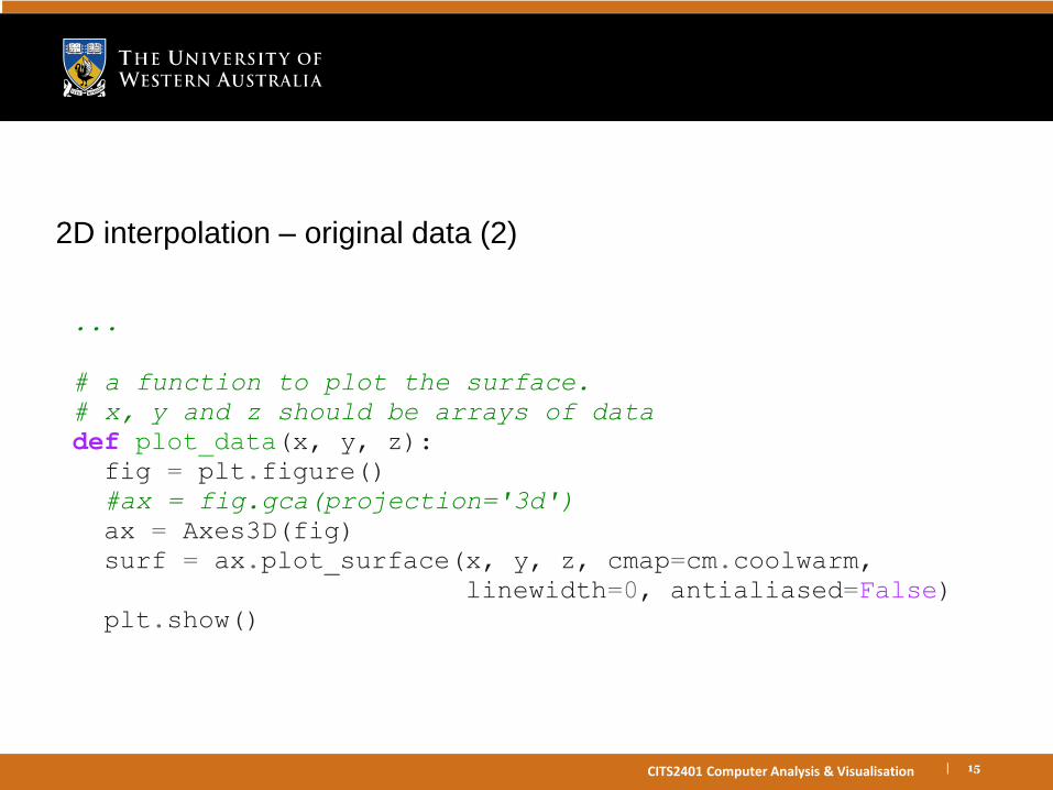
2D interpolation – original data (2)
...
# a function to plot the surface.
# x, y and z should be arrays of data
def plot_data(x, y, z):
fig = plt.figure()
#ax = fig.gca(projection='3d')
ax = Axes3D(fig)
surf = ax.plot_surface(x, y, z, cmap=cm.coolwarm,
linewidth=0, antialiased=False)
plt.show()
| 16CITS2401 Computer Analysis & Visualisation
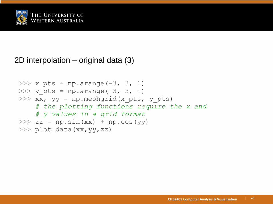
2D interpolation – original data (3)
>>> x_pts = np.arange(-3, 3, 1)
>>> y_pts = np.arange(-3, 3, 1)
>>> xx, yy = np.meshgrid(x_pts, y_pts)
# the plotting functions require the x and
# y values in a grid format
>>> zz = np.sin(xx) + np.cos(yy)
>>> plot_data(xx,yy,zz)
| 17CITS2401 Computer Analysis & Visualisation
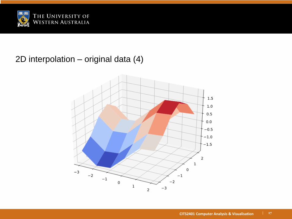
2D interpolation – original data (4)

| 18CITS2401 Computer Analysis & Visualisation
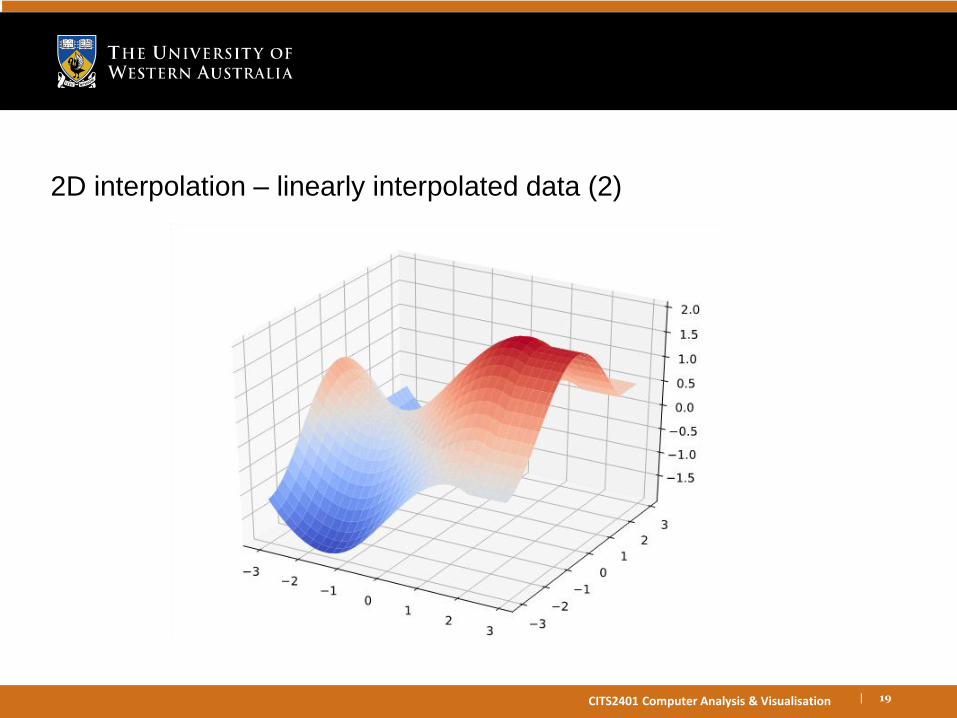
2D interpolation – linearly interpolated data
Now we'll perform linear interpolation.
interpolate.interp2d(x, y, z, kind='linear') returns a
function which, when called, returns the actual interpolated values.
>>> from scipy import interpolate
>>> f = interpolate.interp2d(x_pts, y_pts, zz, kind='linear')
# "kind" specifies whether we're doing linear, cubic, etc.
>>> x_vals = np.arange(-3, 3, 0.1)
>>> y_vals = np.arange(-3, 3, 0.1)
>>> xx_v, yy_v = np.meshgrid(x_vals, y_vals)
>>> zz_v = f(x_vals, y_vals)
>>> plot_data(xx_v,yy_v,zz_v)
| 19CITS2401 Computer Analysis & Visualisation
2D interpolation – linearly interpolated data (2)
| 20CITS2401 Computer Analysis & Visualisation
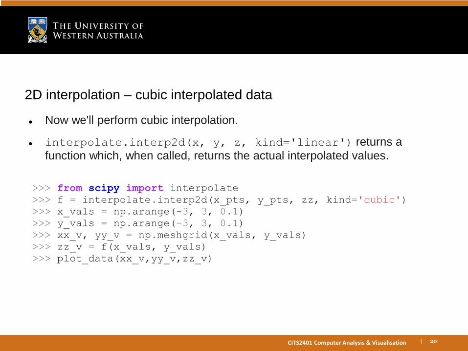
2D interpolation – cubic interpolated data
Now we'll perform cubic interpolation.
interpolate.interp2d(x, y, z, kind='linear') returns a
function which, when called, returns the actual interpolated values.
>>> from scipy import interpolate
>>> f = interpolate.interp2d(x_pts, y_pts, zz, kind='cubic')
>>> x_vals = np.arange(-3, 3, 0.1)
>>> y_vals = np.arange(-3, 3, 0.1)
>>> xx_v, yy_v = np.meshgrid(x_vals, y_vals)
>>> zz_v = f(x_vals, y_vals)
>>> plot_data(xx_v,yy_v,zz_v)

| 21CITS2401 Computer Analysis & Visualisation
2D interpolation – cubic interpolated data (2)

| 22CITS2401 Computer Analysis & Visualisation
Curve fitting
Collected data always contains some degree of error or imprecision
Whereas interpolation is used when we assume that all data points are accurate and we want to infer new intermediate data points –curve fitting is used when we want to match an analytical (or symbolic) model to a set of measurements which may contain some error.
| 23CITS2401 Computer Analysis & Visualisation
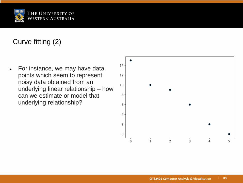
Curve fitting (2)
For instance, we may have data points which seem to represent noisy data obtained from an underlying linear relationship – how can we estimate or model that underlying relationship?
| 24CITS2401 Computer Analysis & Visualisation
Linear regression
One method of curve fitting is linear regression – it minimizes the "square of the errors" (where the "error" is the distance each point is from the line).
(In Excel, there is a function called "SLOPE" which performs linear regression on a set of data points, similar to the Python functions we will see here.)
| 25CITS2401 Computer Analysis & Visualisation
Polynomial regression
Linear regression is a special case of polynomial regression –
since a line (i.e., an equation of the form ax + b) is a simple polynomial.
But your data may not reflect a linear relationship – a polynomial of a higher order may be a better fit.
| 26CITS2401 Computer Analysis & Visualisation
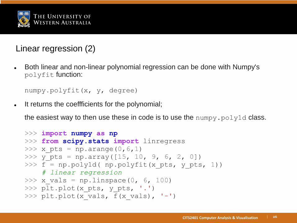
Linear regression (2)
Both linear and non-linear polynomial regression can be done with Numpy's polyfit function:
numpy.polyfit(x, y, degree)
It returns the coeffficients for the polynomial;
the easiest way to then use these in code is to use the numpy.poly1d class.
>>> import numpy as np
>>> from scipy.stats import linregress
>>> x_pts = np.arange(0,6,1)
>>> y_pts = np.array([15, 10, 9, 6, 2, 0])
>>> f = np.poly1d( np.polyfit(x_pts, y_pts, 1))
# linear regression
>>> x_vals = np.linspace(0, 6, 100)
>>> plt.plot(x_pts, y_pts, '.')
>>> plt.plot(x_vals, f(x_vals), '-')
| 27CITS2401 Computer Analysis & Visualisation
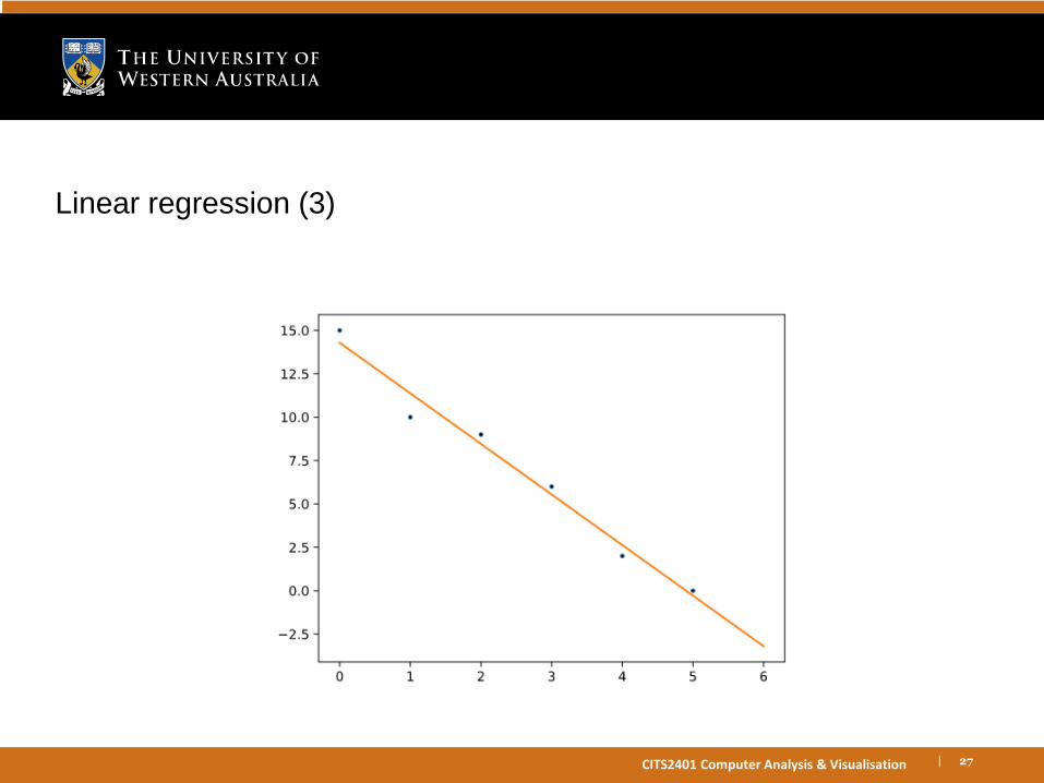
Linear regression (3)
| 28CITS2401 Computer Analysis & Visualisation
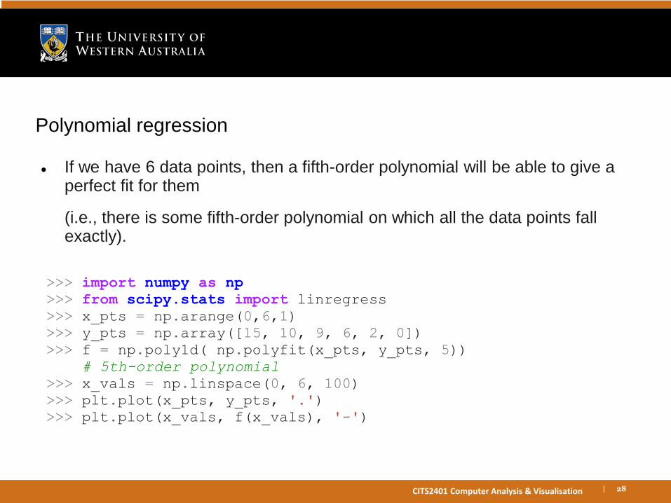
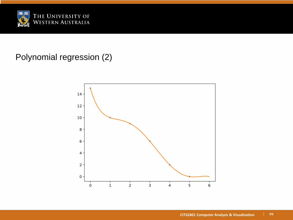
Polynomial regression
If we have 6 data points, then a fifth-order polynomial will be able to give a perfect fit for them
(i.e., there is some fifth-order polynomial on which all the data points fall exactly).
>>> import numpy as np
>>> from scipy.stats import linregress
>>> x_pts = np.arange(0,6,1)
>>> y_pts = np.array([15, 10, 9, 6, 2, 0])
>>> f = np.poly1d( np.polyfit(x_pts, y_pts, 5))
# 5th-order polynomial
>>> x_vals = np.linspace(0, 6, 100)
>>> plt.plot(x_pts, y_pts, '.')
>>> plt.plot(x_vals, f(x_vals), '-')
| 29CITS2401 Computer Analysis & Visualisation
Polynomial regression (2)
| 30CITS2401 Computer Analysis & Visualisation
Interpolation and curve fitting – part 2

| 31CITS2401 Computer Analysis & Visualisation
Overview
Multiple variable regression
Non-linear terms in regression
| 32CITS2401 Computer Analysis & Visualisation
Multiple variable data
In our regression examples, we have used models where a single output variable changes with respect to a single input variable.But real data may have multiple input variables.
For example, the top speed of a vehicle will depend on many variables such as engine size, weight, air resistance etc.
| 33CITS2401 Computer Analysis & Visualisation
Predictor and response variables
The input variables are called the
independent variables, OR
predictor variables, OR
experimental variables
The output variable is referred to as the
dependent variable, OR
response variable, OR
outcome variable
| 34CITS2401 Computer Analysis & Visualisation
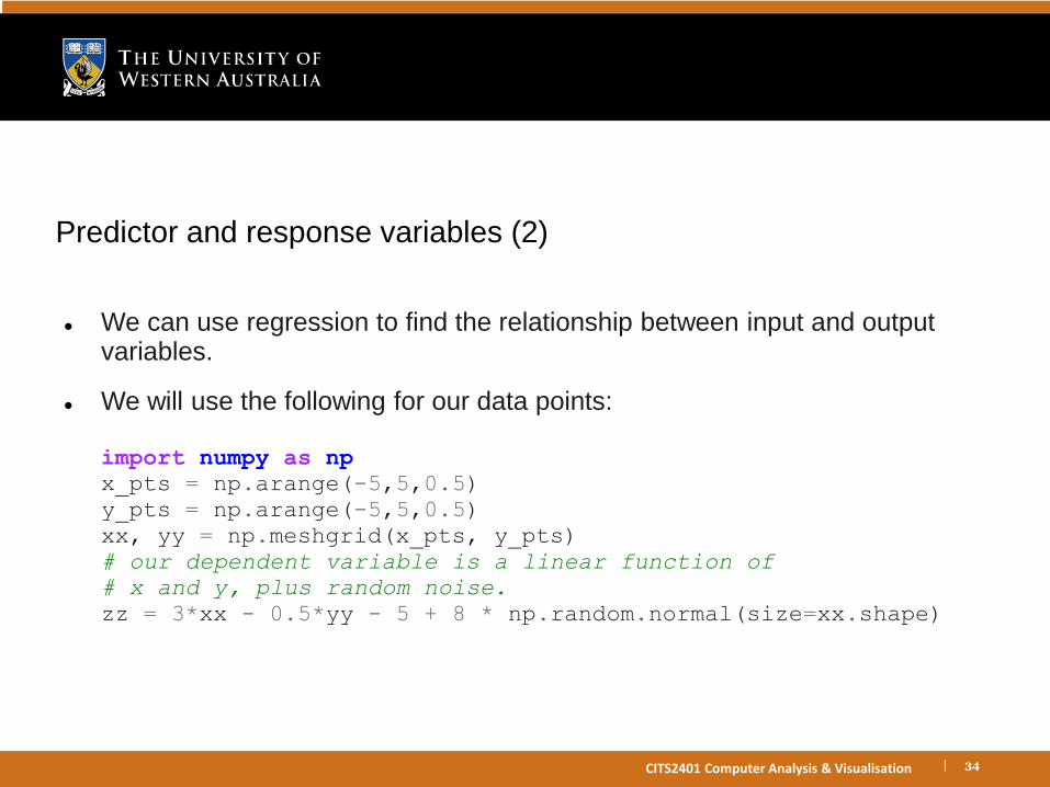
Predictor and response variables (2)
We can use regression to find the relationship between input and output variables.
We will use the following for our data points:
import numpy as np
x_pts = np.arange(-5,5,0.5)
y_pts = np.arange(-5,5,0.5)
xx, yy = np.meshgrid(x_pts, y_pts)
# our dependent variable is a linear function of
# x and y, plus random noise.
zz = 3*xx - 0.5*yy - 5 + 8 * np.random.normal(size=xx.shape)
| 35CITS2401 Computer Analysis & Visualisation
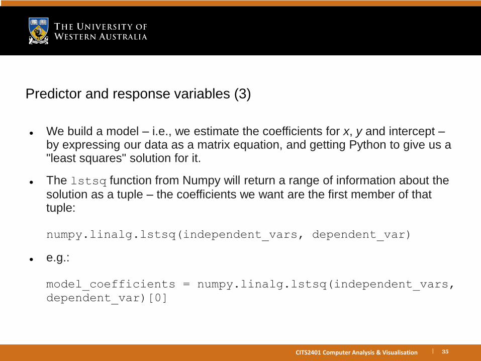
Predictor and response variables (3)
We build a model – i.e., we estimate the coefficients for x, y and intercept –by expressing our data as a matrix equation, and getting Python to give us a "least squares" solution for it.
The lstsq function from Numpy will return a range of information about the solution as a tuple – the coefficients we want are the first member of that tuple:
numpy.linalg.lstsq(independent_vars, dependent_var)
e.g.:
model_coefficients = numpy.linalg.lstsq(independent_vars,
dependent_var)[0]
| 36CITS2401 Computer Analysis & Visualisation
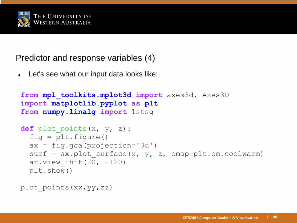
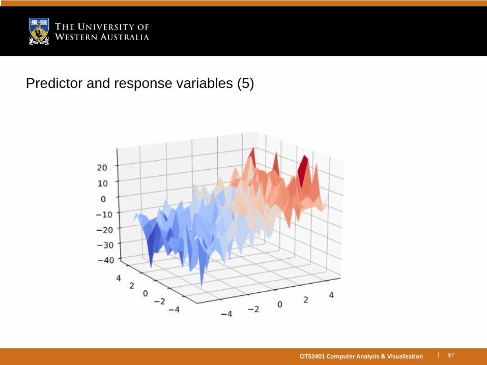
Predictor and response variables (4)
Let's see what our input data looks like:
from mpl_toolkits.mplot3d import axes3d, Axes3D
import matplotlib.pyplot as plt
from numpy.linalg import lstsq
def plot_points(x, y, z):
fig = plt.figure()
ax = fig.gca(projection='3d')
surf = ax.plot_surface(x, y, z, cmap=plt.cm.coolwarm)
ax.view_init(20, -120)
plt.show()
plot_points(xx,yy,zz)
| 37CITS2401 Computer Analysis & Visualisation
Predictor and response variables (5)
| 38CITS2401 Computer Analysis & Visualisation
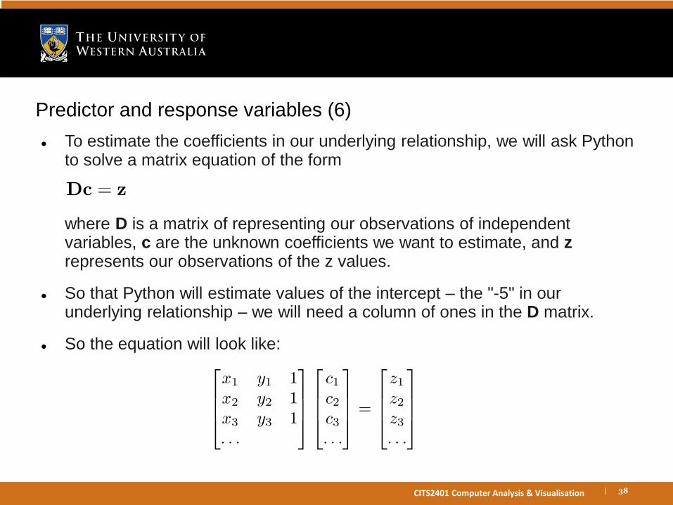
Predictor and response variables (6)
To estimate the coefficients in our underlying relationship, we will ask Python to solve a matrix equation of the form
where D is a matrix of representing our observations of independent variables, c are the unknown coefficients we want to estimate, and zrepresents our observations of the z values.
So that Python will estimate values of the intercept – the "-5" in our underlying relationship – we will need a column of ones in the D matrix.
So the equation will look like:
| 39CITS2401 Computer Analysis & Visualisation
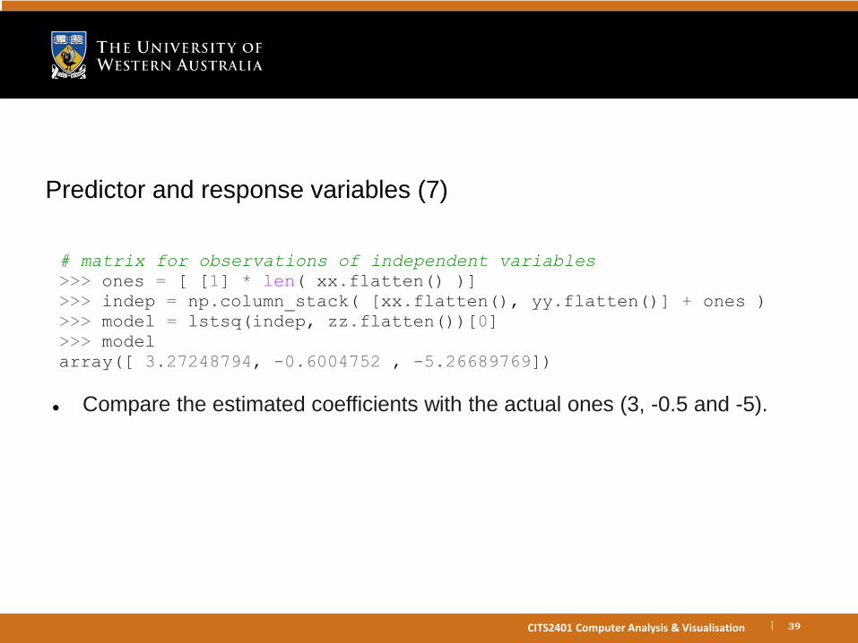
Predictor and response variables (7)
# matrix for observations of independent variables
>>> ones = [ [1] * len( xx.flatten() )]
>>> indep = np.column_stack( [xx.flatten(), yy.flatten()] + ones )
>>> model = lstsq(indep, zz.flatten())[0]
>>> model
array([ 3.27248794, -0.6004752 , -5.26689769])
Compare the estimated coefficients with the actual ones (3, -0.5 and -5).
| 40CITS2401 Computer Analysis & Visualisation
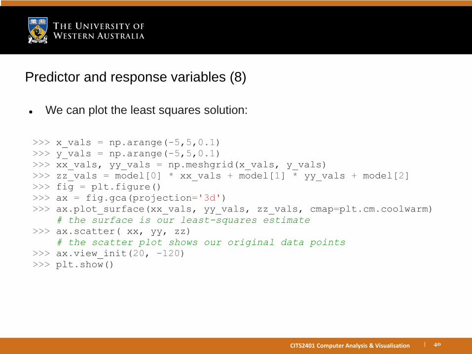
Predictor and response variables (8)
We can plot the least squares solution:
>>> x_vals = np.arange(-5,5,0.1)
>>> y_vals = np.arange(-5,5,0.1)
>>> xx_vals, yy_vals = np.meshgrid(x_vals, y_vals)
>>> zz_vals = model[0] * xx_vals + model[1] * yy_vals + model[2]
>>> fig = plt.figure()
>>> ax = fig.gca(projection='3d')
>>> ax.plot_surface(xx_vals, yy_vals, zz_vals, cmap=plt.cm.coolwarm)
# the surface is our least-squares estimate
>>> ax.scatter( xx, yy, zz)
# the scatter plot shows our original data points
>>> ax.view_init(20, -120)
>>> plt.show()

| 41CITS2401 Computer Analysis & Visualisation
Predictor and response variables (9)

| 42CITS2401 Computer Analysis & Visualisation
Curve-fitting using non-linear terms in linear regression
What if we have a non-linear relationship between our variables?
We can actually still use linear regression, as we did in the previous example: but in our matrix of independent variables, we'll include terms which are a non-linear function of our observations.
>>> xx_flat = xx.flatten()
>>> yy_flat = yy.flatten()
>>> zz_flat = zz.flatten()
>>> ones = [ [1] * len( xx_flat )]
>>> indep = np.column_stack( [xx_flat, yy_flat,
3 * np.sin(2 * xx_flat) ] + ones )
# the 3rd column is *3sin(2x)*
>>> model = lstsq(indep, zz.flatten())[0]
>>> model
array([ 2.88268949, -0.30450846, -0.02530611, -4.46351387])
| 43CITS2401 Computer Analysis & Visualisation
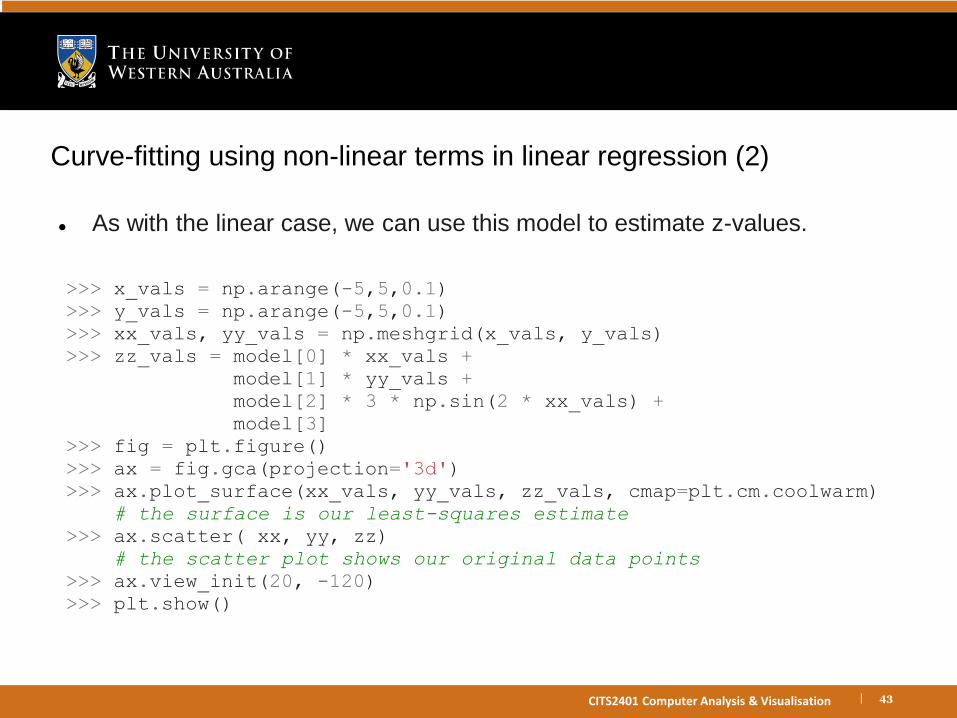
Curve-fitting using non-linear terms in linear regression (2)
As with the linear case, we can use this model to estimate z-values.
>>> x_vals = np.arange(-5,5,0.1)
>>> y_vals = np.arange(-5,5,0.1)
>>> xx_vals, yy_vals = np.meshgrid(x_vals, y_vals)
>>> zz_vals = model[0] * xx_vals +
model[1] * yy_vals +
model[2] * 3 * np.sin(2 * xx_vals) +
model[3]
>>> fig = plt.figure()
>>> ax = fig.gca(projection='3d')
>>> ax.plot_surface(xx_vals, yy_vals, zz_vals, cmap=plt.cm.coolwarm)
# the surface is our least-squares estimate
>>> ax.scatter( xx, yy, zz)
# the scatter plot shows our original data points
>>> ax.view_init(20, -120)
>>> plt.show()

| 44CITS2401 Computer Analysis & Visualisation
Curve-fitting using non-linear terms in linear regression (3)