International Trade Network: Country centrality

and COVID-19 pandemic

Roberto Antonietti∗1, Paolo Falbo†2, Fulvio Fontini‡1, RosannaGrassi §2, and Giorgio Rizzini ¶2

1Department of Economics and Management ”Marco Fanno”,University of Padova, Padova, Italy

2Department of Economics and Management, University ofBrescia, Brescia, Italy

3Department of Statistics and Quantitative Methods, University ofMilano - Bicocca, Milan, Italy

Keywords: World Trade Network; Centrality Measures; Community De-tection; COVID-19

JEL classification: F11; F14; F62MSC 2010 classification: 91B60; 05C82; 62P20

Abstract

International trade is based on a set of complex relationships betweendifferent countries that can be modelled as an extremely dense networkof interconnected agents. On the one hand, this network might favourthe economic growth of countries, but on the other, it can also favour thediffusion of diseases, like the COVID-19. In this paper, we study whether,and to what extent, the topology of the trade network can explain therate of COVID-19 diffusion and mortality across countries. We computethe countries’ centrality measures and we apply the community detectionmethodology based on communicability distance. Then, we use thesemeasures as focal regressors in a negative binomial regression framework.In doing so, we also compare the effect of different measures of centrality.Our results show that the number of infections and fatalities are larger incountries with a higher centrality in the global trade network.

∗roberto.antonietti@unipd.it†paolo.falbo@unibs.it‡fulvio.fontini@unipd.it§rosanna.grassi@unimib.it¶giorgio.rizzini@unimib.it

1

arX

iv:2

107.

1455

4v1

[ec

on.G

N]

30

Jul 2

021

1 Introduction

At the beginning of 2020, the COVID-19 disease rapidly diffused from the localChinese region of Hubei, becoming soon a global health emergency. Since itoriginated in a highly populated region, strategic for several industrial sectors,the effects of lockdown restrictions led to a freezing of business investments anda reduction in Chinese household consumption, which had a significant impacton Chinese trades. Rapidly, the spreading of the COVID-19 disease has severelyaffected all the economies in the world.

Understanding the factors that triggered the COVID-19 outbreak is stillan object of debate. The spread of a pandemic is a complex matter and canbe affected by several factors. Much of the complexity is that many of thesefactors interact. In the case of COVID-19, the aerosol droplets spreading withnormal breathing and talking when two or more individuals meet physically,has been identified as the main contagion mechanism. Keeping 1.5 or moremeters of distance between individuals reduces the risk of contagion. However,despite their necessity, physical explanations seem to provide only a part ofthe reasons explaining the ongoing COVID-19 pandemic. The reasons and theopportunities to bring people to travel around the world, to spend time meetingother people seem more crucial to this purpose. Different business, social and(or) family reasons discriminate much more effectively the chances for peopleto enter physically in contact with each other, at both global and local scales.Economic and social factors seem to provide much more explanatory power tounderstand the COVID-19 pandemic.

In this paper we stress the role of international trade, and specifically ofthe countries’ central position in the global trade scenario. From a topologi-cal point of view, the commercial trades between countries are characterizedby an intricate weave of relations, and the complex network theory offers aneffective representation of this situation. Both connections between countriesand bilateral trade flows can be modelled as a dense network of interconnectedagents. Assessing the role of these strong interconnections on the dynamics ofthe COVID-19 diffusion, and mortality, during the first wave (between Marchand April 2020) is therefore an interesting research question.

However, a major difficulty arises in the search of such interconnections.More precisely, since the trade network is naturally dense and almost complete,the study of the classical global network indicators applied to the whole networkare not informative enough. This suggests an accurate choice of more effectivenetwork tools.

In this view, a first aim of the paper is to assess the countries centralityas well as to identify a more satisfactory representation of the internationaltrade landscape. Focusing on years 2019 and 2020, such analyses should allowus to detect and describe more precisely if any changes in the internationaltrade network have eventually occurred as a consequence of the COVID-19. Indoing so, we focus on those measures that are meaningful in capturing possiblemodifications. A second aim is to assess if such centrality measures also have anyexplanatory power with respect to the huge differences in the rate of infection,

2

and mortality that have been observed worldwide, once controlled for a seriesof other confounding factors.

Some works in the literature suggest that the level of mobility of people (bothat international and local levels) has played a role in the COVID-19 pandemic.As pointed out in Antonietti et al. (2021) and Fernandez-Villaverde and Jones(2020), an intensive international mobility of people (for business or tourismreasons) can explain the different infection and mortality rates across countries.More precisely, countries with higher level of inward international mobility havehigher probabilities to anticipate the time of the first contagions and to havehigher number of infected people freely circulating during the pre-symptomsperiod. When on March 12th, 2020, the World Health Organization (WHO)announced the COVID-19 pandemic outbreak, both the contagion and mortal-ity rates were already much different from country to country, with China andsome EU countries already severely hit. Russo et al. (2020) point to January18th as day-zero of the COVID-19 outbreak in Lombardy (Italy), which hasbeen one of the mostly hit regions worldwide. Parodi and Aloisi (2020) suspectthat the abnormal number of cases of bilateral pneumonia occurred in Lom-bardy already in December 2019 could be attributed to COVID-19. A factorthat increases the probability of early contagion in a region, or a country, iscertainly the movement of the citizens outside and inside its borders. In theircross-sectional analysis based on the Spanish regions, Paez et al. (2020) observethat local public mass transportation system, more than international airportfacilities, appears a factor linked to higher severity of contagion rates. Inter-national and local transports seem to act differently. The former increases thechances of early contagion events, while the latter plays a second-order conta-gion enhancer.International trade data can be used as a comprehensive indicator accounting forpopulation density, economic dynamism, and human mobility. In this regards,Bontempi and Coccia (2021) investigate the relations between the total importand export of 107 provinces of Italy and the COVID-19 transmission dynamics.Extending the previous work, Bontempi et al. (2021) focus the regional data ofFrance, Italy and Spain and confirm the relevance of trade in the analysis ofCOVID-19 pandemic, finding strong positive correlation between the interna-tional trade volume of each region and the percentage of patients recovered inthe intensive care units.From a network perspective, the impact of topology and metric properties onthe stability and resilience of an economic or financial system has been widelystudied in the literature, see e.g. Kali and Reyes (2007); Piccardi and Tajoli(2018).On the one hand, community detection is an useful tool to see how an externalshock modifies the topological structure of complex systems (Fortunato and Hric(2016)). On the other hand, a suitable metric can highlight the role of non-localinteractions between nodes. In this regard, Estrada and Hatano (2008, 2009)introduce the concept of communicability, presenting a metric between nodesthat takes into consideration long-range interactions between them.An area in which these concepts allow us to gain a deep insight into the hidden

3

structures of the network is properly the World Trade Network (WTN), seeBartesaghi et al. (2020).The topology of the WTN has been extensively analyzed over time. The behav-ior of international trade flows, the impact of globalization on the internationalexchanges, the presence of a core-periphery structure or the evolution of thecommunity centres of trade, are just some of the issues addressed by the re-cent developments (see Serrano et al. (2007); Tzekina et al. (2008); Fagioloet al. (2010); De Benedictis and Tajoli (2011); Blochl et al. (2011); Grassi et al.(2021)). Recently, some works correlate the commercial trades with the COVID-19 diffusion from a network point of view (Antonietti et al. (2020); Reissl et al.(2021); Kiyota (2021); Fagiolo (2020).Such results further motivate the analysis of the link between COVID-19 pan-demic and the trade networks among countries.

Our contribution to the literature is twofold. Firstly, we detect more pre-cisely the presence of trade communities not only via their direct connections,as measured by the total volume of trade directly exchanged between two coun-tries, but also via indirect connections. Indeed, we argue that it is crucial toconsider deep interconnections between nodes, in order to capture the strategiccommercial links, which can survive beyond a global shock. To this end, we ap-ply the recent methodology proposed by Bartesaghi et al. (2020) focusing on theEstrada communicability distance (Estrada and Hatano (2009)). As a result,the analysis of communities performed in 2019 and 2020 shows that the tradenetwork is a resilient structure, adapting itself to a global shock such as a pan-demic. Secondly, we provide strong empirical evidence that, on the contrary, thenetwork centrality measures have impacted to the early diffusion and mortalityrates of COVID-19. We show in particular that a higher country centrality inthe WTN corresponds to a higher risk of infection and death. Also, the com-munity clustering coefficient, that synthesizes both the community structureand countries centrality, leads to a higher number of deaths and infections withrespect to the ones computed with the classical clustering coefficient.

The paper is organized as follows: in section 2 we describe the methodologyand the network indicators, as well as the econometric model used to perform theanalysis. In section 3 we describe the WTN and socio-economic data used andhow we constructed the world trade network. In section 4 we report and discussthe results of the network analysis and the econometric model. Conclusionsfollow in section 5.

2 Methodology and network indicators

In this section we describe the methodology that we apply in the paper, inparticular the community detection method, as well as the centrality measuresused later for the econometric analysis.

Firstly, we briefly remind some preliminary definitions. A network is formallyrepresented by a graph G = (V,E) where V and E are the sets of n nodes andm edges (or links), respectively. We consider simple graphs without self-loops.

4

Two nodes i and j are adjacent if there is an edge (i, j) ∈ E connecting them.If (i, j) ∈ E implies (j, i) ∈ E then the network is undirected. A walk of lengthk is a sequence of adjacent vertices v0, v2, ..., vk. When all vertices in a walkare distinct, the walk is a path. A i − j geodesic is the shortest path betweenvertices i and j. The length of the i− j geodesic is the distance d(i, j) betweeni and j. Adjacency relationships are represented by the adjacency matrix A,whose elements aij are equal to 1 if (i, j) ∈ E and zero otherwise. We denotewith λ1 ≥ λ2 ≥ · · · ≥ λn the eigenvalues of A and ρ = maxi (|λ|i) its spectralradius. By the Perron-Frobenius Theorem Horn and Johnson (2012) ρ is aneigenvalue of A and there exists a positive eigenvector x such that Ax = ρx.Such an eigenvector x is called principal eigenvector.The ij-entry of the kth power of the adjacency matrix Ak provides the numberof walks of length k starting at i and ending at j. We define the degree di asthe number of edges adjacent to i.

A graph G is weighted when a positive real number wij > 0 is associatedwith the edge (i, j). In this case, the adjacency matrix is a non-negative matrixW. We define the strength si as the sum of the weights of the edges adjacentto i and the diagonal matrix whose diagonal entries are si is S.

2.1 Community detection based on communicability dis-tance

We describe here the community detection method using the Estrada communi-cability distance proposed in Bartesaghi et al. (2020). We focus here on the mainsteps of the methodology. For a detailed description of the proposed methodol-ogy, we refer the reader to Bartesaghi et al. (2020).The main idea is to detect communities by optimizing a quality function thatexploits the additional information contained in a metric structure based on theEstrada communicability. At first, we recall the definition of Estrada communi-cability (simply, communicability) between two nodes i and j (see Estrada andHatano (2008)):

Gij =

+∞∑k=0

1

k![Ak]ij =

[eA]ij. (1)

As the ij-entry of the k-power of the adjacency matrix A provides the num-ber of walks of length k starting at i and ending at j, Gij accounts for all channelsof communication between two nodes, giving more weight to the shortest routesconnecting them. The elements Gii, i = 1, ..., n are known in the literatureas subgraph centrality Estrada and Rodriguez-Velazquez (2005). The commu-nicability matrix is then the exponential of the matrix A, simply denoted byG.

In the case of a weighted network, the weighted communicability function isdefined as

5

Gij =

+∞∑k=0

1

k![(S−

12 WS−

12 )k]ij =

[e(S− 1

2 WS−12 )

]ij

(2)

Following Crofts and Higham (2009), the matrix W in formula (2) has beennormalized to avoid the excessive influence of links with higher weights in thenetwork.

Using the communicability, a meaningful distance metric ξij can be con-structed, as defined in Estrada (2012):

ξij = Gii − 2Gij +Gjj . (3)

By definition of communicability, Gij measures the amount of informationtransmitted from the node i to j. On the other hand, Gii measures the im-portance of a node according to its participation in all closed walks to which itbelongs. Hence, in terms of information diffusion, Gii is the amount of infor-mation that, after flowing along closed walks, returns to the node i.

Thus, the quantity ξij accounts for the difference in the amount of informa-tion that returns to the nodes i and j and the amount of information exchangedbetween them. The greater is Gij , the larger the information exchanged and thenearer are the nodes; the greater are Gii or Gjj , the larger the information thatcomes back to the nodes and the farther are the nodes. Since ξij is a metric,then Gii + Gjj ≥ 2Gij , i.e., no matter what the structure of the network is,the amount of information absorbed by a pair of nodes is always larger or equalthan the amount of information transmitted between them.The metric is meaningful if we apply it to international trade network. In-deed, network flows along links measure how well two countries communicate interms of commercial exchanges. For instance, the link between two nodes maybe identified with the total trade or money flow between two countries.

We assume that two nodes are considered members of the same communityif their mutual distance ξij is lower than a threshold ξ0 ∈ [ξmin, ξmax]. Inparticular, we construct a new community graph with adjacency matrix M =[mij ] given by:

mij =

1 if ξij ≤ ξ00 otherwise

(4)

In this way, clustered groups of nodes that “strongly communicate” emerge,varying the threshold ξ0.

As well explained in Bartesaghi et al. (2020), ξ0 is not arbitrarily chosen,but it is obtained by solving the following optimization problem

ξ0 ∈ arg maxQ.

The objective function Q is

Q =∑i,j

γijxij , (5)

6

where xij is a binary variable equal to 1 if nodes i and j belong to the samecommunity and 0 otherwise. γij is a function measuring the cohesion betweennodes i and j. Originally proposed in Chang et al. (2016), it is defined inBartesaghi et al. (2020) as:

γij = (ξj − ξ)− (ξij − ξi), (6)

where ξj is the average distance between node j and nodes other than j andξ is the average distance over the whole network.

Since two nodes are cohesive (incohesive, respectively) if γij ≥ 0 (γij ≤ 0),in terms of distance they are cohesive if they are close to each other and, onaverage, they are both far away from the other nodes.In this perspective, γij can be seen as the “gain” if positive or the “cost” ifnegative, of grouping two nodes i and j in the same community. The appliedmethodology will allow to discover communities in the world trade networkbased on all the possible channels of interactions and exchange between coun-tries.

2.2 Centrality measures

In this section we introduce the centrality measures that will be used in per-forming the econometric analysis.

The centrality of a node indicates its importance in the network Sabidussi(1966). There are several definitions of vertex centrality in a network, dependingon the application. Among them, some measures seem to better capture thecharacteristics of the studied network.The degree centrality, formally expressed by the degree di, quantifies the abilityof a node i to communicate directly with others and it is

di =

n∑j=1

aij . (7)

For weighted networks with weights matrix W, a similar measure is the strengthcentrality si,

si =n∑j=1

wij . (8)

An extension of the degree centrality is the eigenvector centrality (see Bonacich(1972)). Formally, it is represented by the i-th component of the principaleigenvector x of the adjacency matrix:

xi =1

ρ

n∑j=1

aij xj (9)

The eigenvector centrality xi quantifies the connection of a vertex with its neigh-bours that are themselves central. The extension to weighted case is immediate,

7

as the weighted adjacency matrix W preserves all characteristics of A.Betweenness centrality bi, measures the influence that a vertex i has in thespread of information within the network:

bi =∑h,k

ghk(i)

ghk, h, k 6= i (10)

where ghk is the number of h−k geodesic from h to k and ghk(i) is the num-ber of h − k geodesic passing through node i. In the definition of betweennesswe always suppose that the pairs (i, j) appear only once in the sum.

We also consider the local clustering coefficient, which measures the tendencyto which nodes in a network tend to cluster together. Since the world tradenetwork will be represented as an indirect and weighted network (see Section3), we focus on the local weighted coefficient proposed by Onnela et al. (2005):

Ci(W) =

∑j

∑j 6=k w

1/3ij w

1/3jk w

1/3ki

di(di − 1)(11)

where W is the weighted adjacency matrix obtained by normalizing the entrieswij of W as wij =

wij

max(wij)∀i, j. Notice that Ci(W) = Ci represents the geo-

metric mean of the links weights incident to the node i, divided by the numberof potential triangles di centred on it. The main idea is to replace the totalnumber of the triangles in which a node i belongs, with the “intensity” of thetriangle, defined here as the geometric mean of its weights.

2.3 Econometric model

In what follows, we want to assess the role of the WTN on the evolution of thepandemic in the five weeks between March 11th and April 21st 2020. At thesame time, we want to control for additional socio-economic factors that canhave an impact on the diffusion of the pandemic. To avoid the possibility that,in turn, these factors might be affected by COVID-19 diffusion, we include themas referred to year 2019.The baseline model that we adopt to test for the role that Trade NetworkCentrality has played in explaining the number of infections (INF) and deaths(DEATH) in the first wave of the COVID-19 outbreak (i.e., between March 11st,2020 and April 21st, 2020) is the following:

Yit = β0 + β1TNCi + Z′

iβZ + γt + εit (12)

where Yit is either the number of COVID-19 infections (INF) or the numberof deaths (DEATH) in country i and week t. The variable TNCi representsa given trade network centrality measure (respectively: degree in Equation(7), betweenness in Equation (10), local clustering coefficient in Equation (11),

8

weighted eigenvector in Equation (9), and strength in Equation (8)) measuredin 2019; Z is a vector of additional regressors that can explain the number ofinfections and fatalities due to COVID-19, namely GDP per capita (GDPPC, atconstant 2010 US$), total resident population (POP), the share of elderly popu-lation (POP65+), the number of hospital beds per 1,000 inhabitants (HBEDS),and the average temperature in February and March (in degree Celsius), allmeasured in 2019. The term γt is a vector including a set of five week-specificdummies that capture the trend in the dynamics of COVID-19 infections andfatalities for all our countries, while εit is the stochastic error component withzero mean and finite variance σ2

ε . Since the residuals of Equation (12) are likelyto be correlated within countries, we cluster the standard errors at the countrylevel. Since Yit is a count variable, and our regressors are time-invariant becausethey are all measured in 2019, we estimate Equation (12) using a pooled nega-tive binomial regression model. As common for count-data models, we test forthe overdispersion of our data, that is, for the fact that the conditional meancan be lower than the conditional variance, typically due to the presence of un-observed factors than can affect the number of COVID-19 infections or deaths.In such a case, the main assumption for the use of the Poisson model is violated,and the negative binomial model is more suited to estimate Equation (12).We also check for the presence of potential multicollinearity by re-estimatingEquation (12) through a linear regression model and using a Variance Infla-tion Factor (VIF) statistic 1. Multicollinearity can be considered an issue ifthe VIF statistic takes a value higher than the commonly accepted threshold of5. To check which of the proposed trade network centrality measures providesthe highest explanatory power in predicting Yit we use the Akaike InformationCriterion (AIC) and Bayesian Information Criterion (BIC).Finally, to compare the magnitude of the estimated coefficients, we standard-ize all the regressors by subtracting their mean and dividing by their standarddeviation. For each variable, we report the incidence rate ratio (IRR) whichmeasures the impact of a unit increase of the regressor on the risk of conta-gion (mortality) from COVID-19, computed as the ratio between the numberof infected (deceased) individuals and the number of non-infected (surviving)individuals. In this respect, the IRR of a regressor is easier to interpret thanthe corresponding estimated coefficient, since this latter is the impact of a unitincrease in the regressor itself on the log of the expected number of infectionsor deaths.

1The VIF is the ratio of variance in a model that uses multiple independent variables andthe variance of a model that uses only one independent variable. This statistic is used to testfor the severity of multicollinearity in linear regressions. For see in detail how VIF statisticworks, we refer for instance to James et al. (2013).

9

3 Data, samples and variables

3.1 Dataset description

The empirical analysis is based on two datasets. The first is used to constructthe network and consists of a sample of monthly trade values during the firstsemester of 2019 and of 2020 for 55 countries listed in Tables 11 and 12 andin the Appendix 1. Data are provided by the Un Comtrade (2021), that is thelargest depository of international trade data. It contains over 40 billion datarecords since 1962 and is available publicly on the internet.The second is used to analyze the relationship that such a trade network haswith COVID-19 diffusion. Data on COVID-19 diffusion come from the TheEuropean Centre for Disease Prevention and Control (2021) (ECDC), an EUagency for the protection of European citizens against infectious diseases andpandemics. The data on the distribution of COVID-19 worldwide are updateddaily by the ECDC’s Epidemic Intelligence team, based on reports providedby national health authorities. Since we are interested in the first wave of thepandemic, we retrieve cross-country daily data on the number of COVID-19infections and deceases, that we pool into five weeks from March 11st, 2020 toApril 21st, 2020.To control for other factors that can potentially affect the diffusion patterns ofCOVID-19, we also consider the following country-level information providedby The World Bank (2021): the real GDP per capita (GDPPC, in 2010 USD)used as a proxy for the average standard of living in a country; the total residentpopulation (POP), taken as a proxy for a country’s size; the share of populationaged 65 or more (POP 65+); the number of hospital beds per capita availablein public, private, general, and specialized hospitals and rehabilitation centers(HBEDS), that we include to capture the average quality of the health systemin each country; the average temperature in February and March (TEMP), indegree Celsius, C.

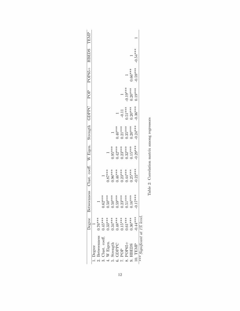
Tables 1 and 2 show the main summary statistics and the pairwise correla-tions among regressors.

3.2 Network construction

Trades between countries are represented as a weighted network, where eachcountry is a node and connections, i.e. links between nodes, is measured by theamount of traded volume (expressed in US-dollars).At first, we compute separately the aggregate trade values of import and exportbetween each pair of countries. Then, we consider a pair of countries (i, j) suchthat both import and export exist. Specifically, focusing on trade flows from ito j, let wimpij and wexpij be the aggregate import trade value and the aggregateexport value, respectively, from i to j. We then put a weighted link from i to jrepresenting the average value between import and export, defined as follows:

10

Variable Mean Std. dev. Min MaxNetwork centralityDegree 50.62 5.223 27 54Betweenness 0.0011 0.0008 0 0.0019Local clustering 0.0022 0.0026 0.0001 0.0122Weighted Eigenvector 0.109 0.198 0.0002 1Strength (:109) 53.71 96.00 0.130 485.9Additional regressorsGDPPC 27085.33 26413.5 809.36 111062.3POP (mln) 53.754 187.62 0.3613 1366.4POP65+ 0.147 0.063 0.026 0.280HBEDS 4.031 2.375 0.600 13.40TEMP (C) 6.181 10.89 -20.99 26.80

Table 1: Summary statistics

wij =

wimp

ij +wexpij

2 if wimpij > 0and wexpij > 0

0 otherwise

Notice that, due to incompleteness of data2, in general wij 6= wji. The resultingnetwork is then weighted and oriented, with eventually bilateral links betweentwo nodes.

Since the approach of Bartesaghi et al. (2020), based on the communicabilitydistance, has been developed on indirect networks, we investigate if it is possibleto neglect the direction of the links. To this end, we compute the Spearmancorrelation between in and out strength distribution for each year of the sample.The resulting correlations is 0.99 for both years. We then can substitute thebilateral arcs between nodes i and j with a single non-oriented link havingweight given by the maximum value between wij and wji, i.e.

wij = max(wij , wji).

This choice is based on an information quality reason: we expected that thehigher is the value traded, the bigger is the information that can contain.

In Table 3 we report the global network indicators referred to the WTN foryears 2019 and 2020.

As expected, the network shows an extremely connected, dense and almostcomplete structure. This is typical of this kind of network, being the economictrades pervasive in all the world. This is certainly confirmed by the average de-gree (51 and 52) and density3 (0.937 and 0.948 for 2019 and 2020, respectively).

2Since we refer to the years 2019 and 2020 not all the countries have completely commu-nicated the data to UN Comtrade

3Density measures how many links between nodes exist compared to how many links be-tween nodes are possible.

11

Deg

ree

Bet

wee

nn

ess

Clu

st.

coeff

.W

Eig

en.

Str

ength

GD

PP

CP

OP

PO

P65+

HB

ED

ST

EM

P1.

Deg

ree

12.

Bet

wee

nn

ess

0.76

***

13.

Clu

st.

coeff

.0.

45**

*0.

62**

*1

4.W

Eig

en.

0.33

***

0.50

***

0.8

7***

15.

Str

engt

h0.

34**

*0.

50**

*0.9

6***

0.9

5***

16.

GD

PP

C0.

48**

*0.

59***

0.4

6***

0.4

2***

0.4

0***

17.

PO

P0.

15**

*0.

23***

0.2

3***

0.2

3***

0.2

1***

-0.1

11

8.P

OP

65+

0.61

***

0.51

***

0.4

4***

0.3

2***

0.3

5***

0.5

1***

-0.1

9***

19.

HB

ED

S0.

36**

*0.

16***

0.2

5***

0.1

5***

0.2

0***

0.2

0***

0.2

0***

0.6

6***

110

.T

EM

P-0

.44*

**-0

.17**

*-0

.22***

-0.2

9***

-0.2

4***

-0.3

6***

0.1

9***

-0.5

9***

-0.5

4***

1***

Sig

nifi

can

tat

1%

leve

l.

Tab

le2:

Corr

elati

on

matr

ixam

on

gre

gre

ssors

12

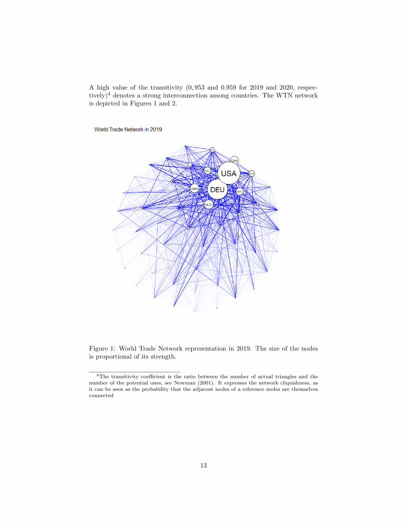
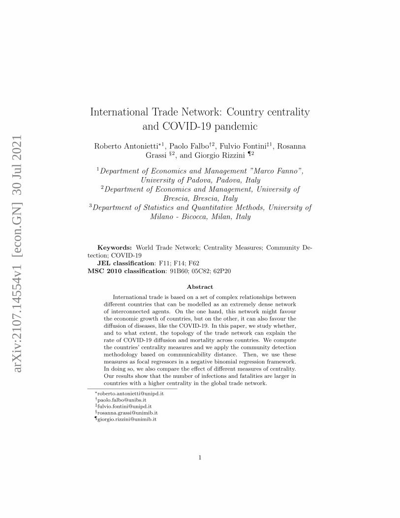
A high value of the transitivity (0, 953 and 0.959 for 2019 and 2020, respec-tively)4 denotes a strong interconnection among countries. The WTN networkis depicted in Figures 1 and 2.

Figure 1: World Trade Network representation in 2019. The size of the nodesis proportional of its strength.

4The transitivity coefficient is the ratio between the number of actual triangles and thenumber of the potential ones, see Newman (2001). It expresses the network cliquishness, asit can be seen as the probability that the adjacent nodes of a reference nodes are themselvesconnected

13

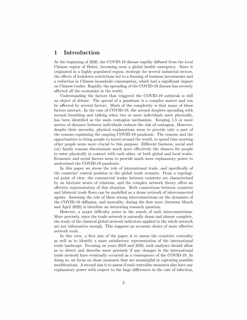
Figure 2: World Trade Network representation in 2020. The size of the nodesis proportional of its strength.

4 Results

4.1 Evolution of WTN during COVID-19

We apply the methodology described in Section 2.1 by using the communicabil-ity distance. As already stressed in the previous Sections, WTN is characterizedby an almost complete structure, where direct connections between countries aredominant. By this approach we have a tool to quantify the depth of the level ofcommunication between countries. Indeed, as pointed out in Bartesaghi et al.(2020), in the WTN two countries are directly connected by a link in terms ofproducts they directly exchange. However, a higher order exchange may occurbetween them, for instance when they are involved in a chain of production.The communicability distance allows us to to take into account trades betweencountries that take place indirectly.

14

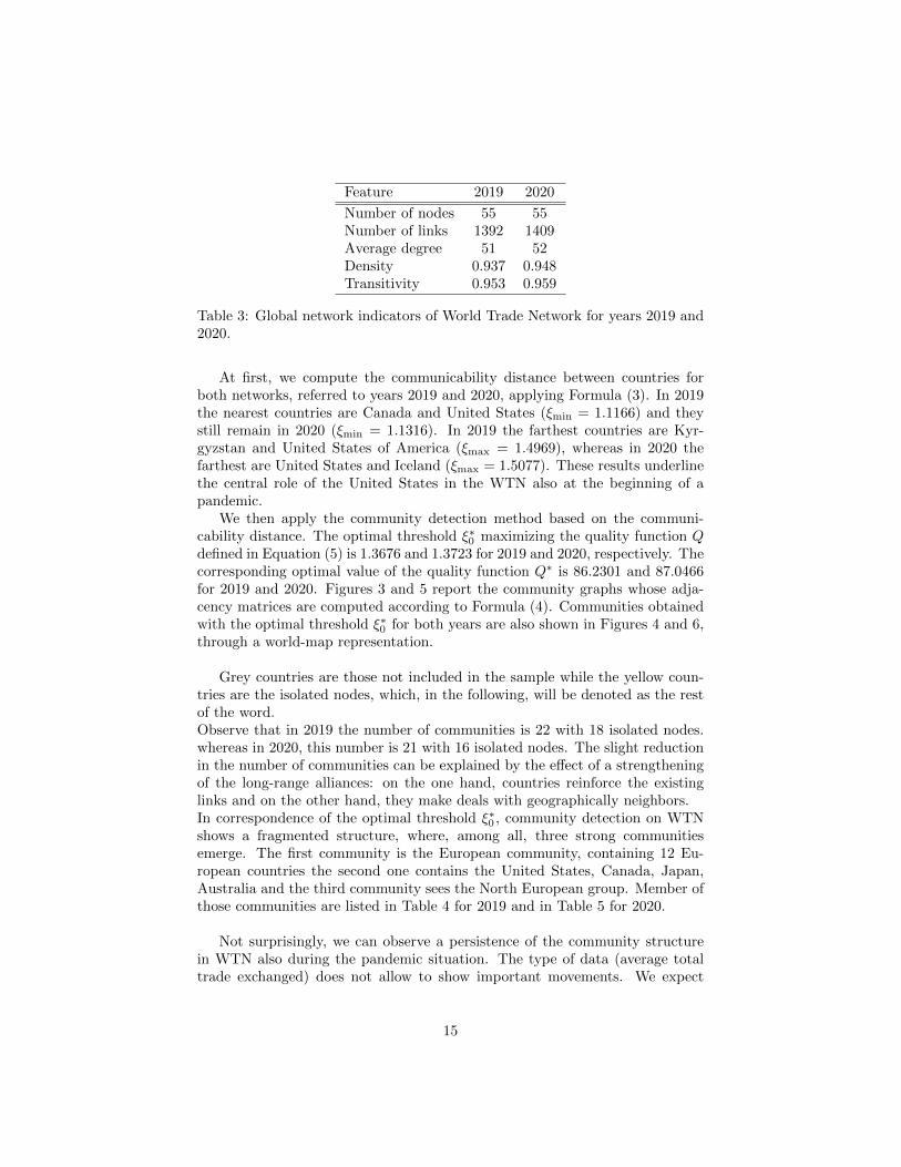
Feature 2019 2020

Number of nodes 55 55Number of links 1392 1409Average degree 51 52Density 0.937 0.948Transitivity 0.953 0.959

Table 3: Global network indicators of World Trade Network for years 2019 and2020.

At first, we compute the communicability distance between countries forboth networks, referred to years 2019 and 2020, applying Formula (3). In 2019the nearest countries are Canada and United States (ξmin = 1.1166) and theystill remain in 2020 (ξmin = 1.1316). In 2019 the farthest countries are Kyr-gyzstan and United States of America (ξmax = 1.4969), whereas in 2020 thefarthest are United States and Iceland (ξmax = 1.5077). These results underlinethe central role of the United States in the WTN also at the beginning of apandemic.

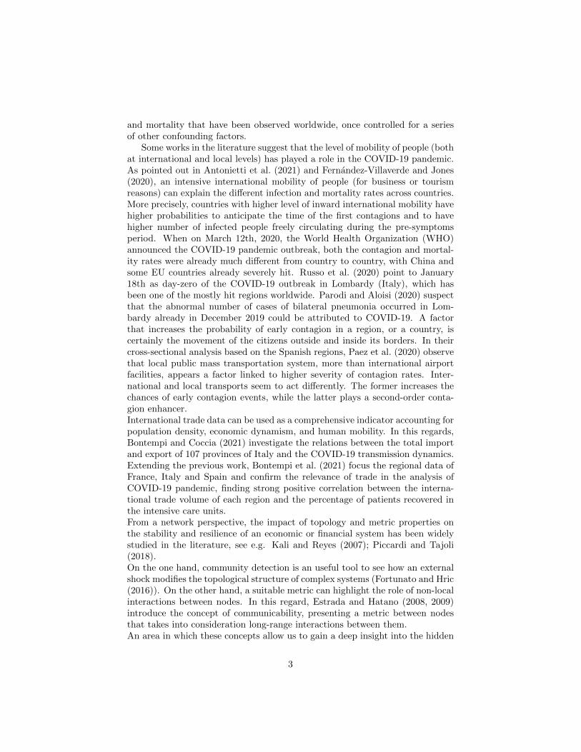
We then apply the community detection method based on the communi-cability distance. The optimal threshold ξ∗0 maximizing the quality function Qdefined in Equation (5) is 1.3676 and 1.3723 for 2019 and 2020, respectively. Thecorresponding optimal value of the quality function Q∗ is 86.2301 and 87.0466for 2019 and 2020. Figures 3 and 5 report the community graphs whose adja-cency matrices are computed according to Formula (4). Communities obtainedwith the optimal threshold ξ∗0 for both years are also shown in Figures 4 and 6,through a world-map representation.

Grey countries are those not included in the sample while the yellow coun-tries are the isolated nodes, which, in the following, will be denoted as the restof the word.Observe that in 2019 the number of communities is 22 with 18 isolated nodes.whereas in 2020, this number is 21 with 16 isolated nodes. The slight reductionin the number of communities can be explained by the effect of a strengtheningof the long-range alliances: on the one hand, countries reinforce the existinglinks and on the other hand, they make deals with geographically neighbors.In correspondence of the optimal threshold ξ∗0 , community detection on WTNshows a fragmented structure, where, among all, three strong communitiesemerge. The first community is the European community, containing 12 Eu-ropean countries the second one contains the United States, Canada, Japan,Australia and the third community sees the North European group. Member ofthose communities are listed in Table 4 for 2019 and in Table 5 for 2020.

Not surprisingly, we can observe a persistence of the community structurein WTN also during the pandemic situation. The type of data (average totaltrade exchanged) does not allow to show important movements. We expect

15

Figure 3: Community graph obtained with communicability distance methodin 2019.

that, focusing on some specific sectors (such as, for example, pharmaceuticalindustry), possible communities changes could be noticed but, at this time, theavailable data does not allow us to do it.Moreover, the analysis period starts from January and ends to June. Thosemonths in 2020 contain only the beginning of COVID-19 pandemic, i.e. the socalled “first wave”. Reasonably, the COVID-19 pandemic situation cannot bereflected immediately on the trade volumes as well as it is not possible to seethe effects of the containment measures.

We now compare the results obtained with the methodology proposed inBartesaghi et al. (2020) with a classical methodology in community detection,the Louvain method Blondel et al. (2008). The method is based on the maxi-mization of a modularity score for each community, where the modularity func-tion quantifies the quality of an assignment of nodes to communities. We observethat the classical method provides a less detailed division in the World TradeNetwork. In both year, we can observe three communities: the first one contain-ing the Europe, the second one contains the USA and Pacific area and the thirdcorresponds to the Northern Europe. Members of communities are plotted inFigures 7 and 8 for the years 2019 and 2020, respectively.

16

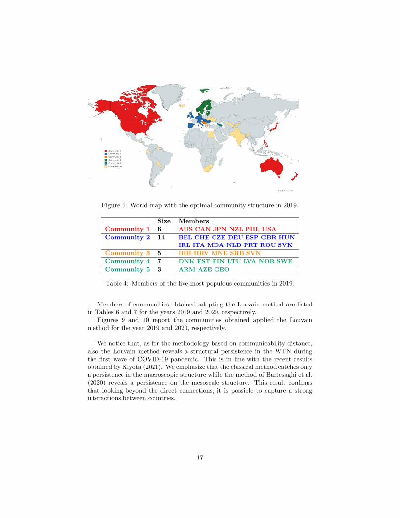
Figure 4: World-map with the optimal community structure in 2019.

Size MembersCommunity 1 6 AUS CAN JPN NZL PHL USA

Community 2 14 BEL CHE CZE DEU ESP GBR HUN

IRL ITA MDA NLD PRT ROU SVK

Community 3 5 BIH HRV MNE SRB SVN

Community 4 7 DNK EST FIN LTU LVA NOR SWE

Community 5 3 ARM AZE GEO

Table 4: Members of the five most populous communities in 2019.

Members of communities obtained adopting the Louvain method are listedin Tables 6 and 7 for the years 2019 and 2020, respectively.

Figures 9 and 10 report the communities obtained applied the Louvainmethod for the year 2019 and 2020, respectively.

We notice that, as for the methodology based on communicability distance,also the Louvain method reveals a structural persistence in the WTN duringthe first wave of COVID-19 pandemic. This is in line with the recent resultsobtained by Kiyota (2021). We emphasize that the classical method catches onlya persistence in the macroscopic structure while the method of Bartesaghi et al.(2020) reveals a persistence on the mesoscale structure. This result confirmsthat looking beyond the direct connections, it is possible to capture a stronginteractions between countries.

17

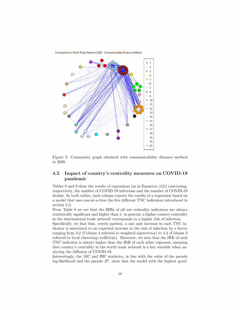
Figure 5: Community graph obtained with communicability distance methodin 2020.

4.2 Impact of country’s centrality measures on COVID-19pandemic

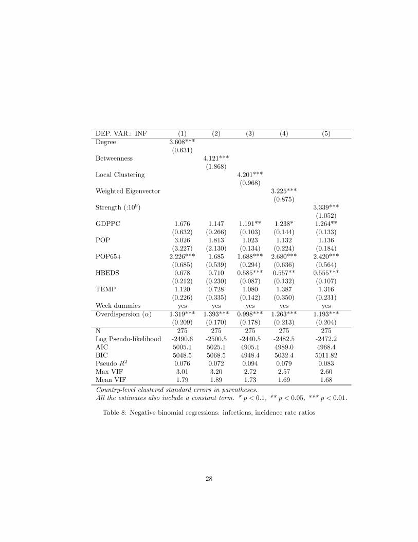
Tables 8 and 9 show the results of regressions (as in Equation (12)) concerning,respectively, the number of COVID-19 infections and the number of COVID-19deaths. In both tables, each column reports the results of a regression based ona model that uses one-at-a-time the five different TNC indicators introduced insection 2.3.From Table 8 we see that the IRRs of all our centrality indicators are alwaysstatistically significant and higher than 1: in general, a higher country centralityin the international trade network corresponds to a higher risk of infection.Specifically, we find that, ceteris paribus, a one unit increase in each TNC in-dicator is associated to an expected increase in the risk of infection by a factorranging from 3.2 (Column 4 referred to weighted eigenvector) to 4.2 (Column 3refereed to local clustering coefficient). Moreover, we note that the IRR of eachTNC indicator is always higher than the IRR of each other regressor, meaningthat country’s centrality in the world trade network is a key variable when an-alyzing the diffusion of COVID-19.Interestingly, the AIC and BIC statistics, in line with the value of the pseudolog-likelihood and the pseudo R2, show that the model with the highest good-

18

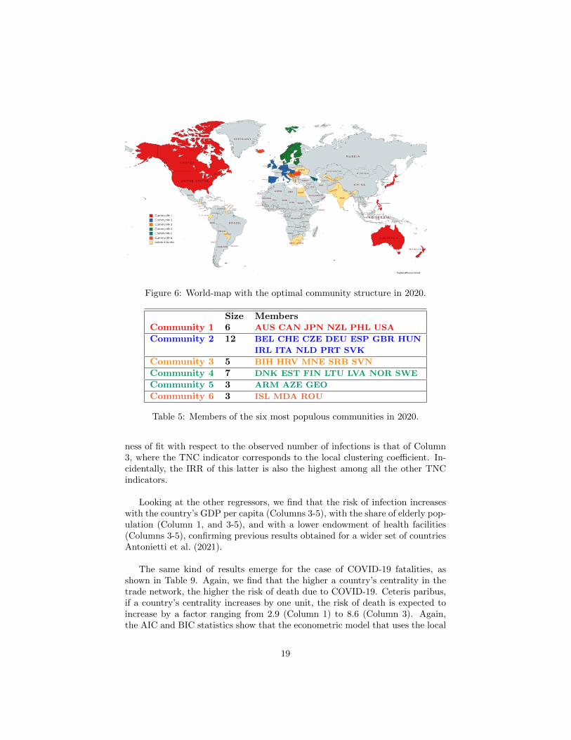
Figure 6: World-map with the optimal community structure in 2020.

Size MembersCommunity 1 6 AUS CAN JPN NZL PHL USA

Community 2 12 BEL CHE CZE DEU ESP GBR HUN

IRL ITA NLD PRT SVK

Community 3 5 BIH HRV MNE SRB SVN

Community 4 7 DNK EST FIN LTU LVA NOR SWE

Community 5 3 ARM AZE GEO

Community 6 3 ISL MDA ROU

Table 5: Members of the six most populous communities in 2020.

ness of fit with respect to the observed number of infections is that of Column3, where the TNC indicator corresponds to the local clustering coefficient. In-cidentally, the IRR of this latter is also the highest among all the other TNCindicators.

Looking at the other regressors, we find that the risk of infection increaseswith the country’s GDP per capita (Columns 3-5), with the share of elderly pop-ulation (Column 1, and 3-5), and with a lower endowment of health facilities(Columns 3-5), confirming previous results obtained for a wider set of countriesAntonietti et al. (2021).

The same kind of results emerge for the case of COVID-19 fatalities, asshown in Table 9. Again, we find that the higher a country’s centrality in thetrade network, the higher the risk of death due to COVID-19. Ceteris paribus,if a country’s centrality increases by one unit, the risk of death is expected toincrease by a factor ranging from 2.9 (Column 1) to 8.6 (Column 3). Again,the AIC and BIC statistics show that the econometric model that uses the local

19

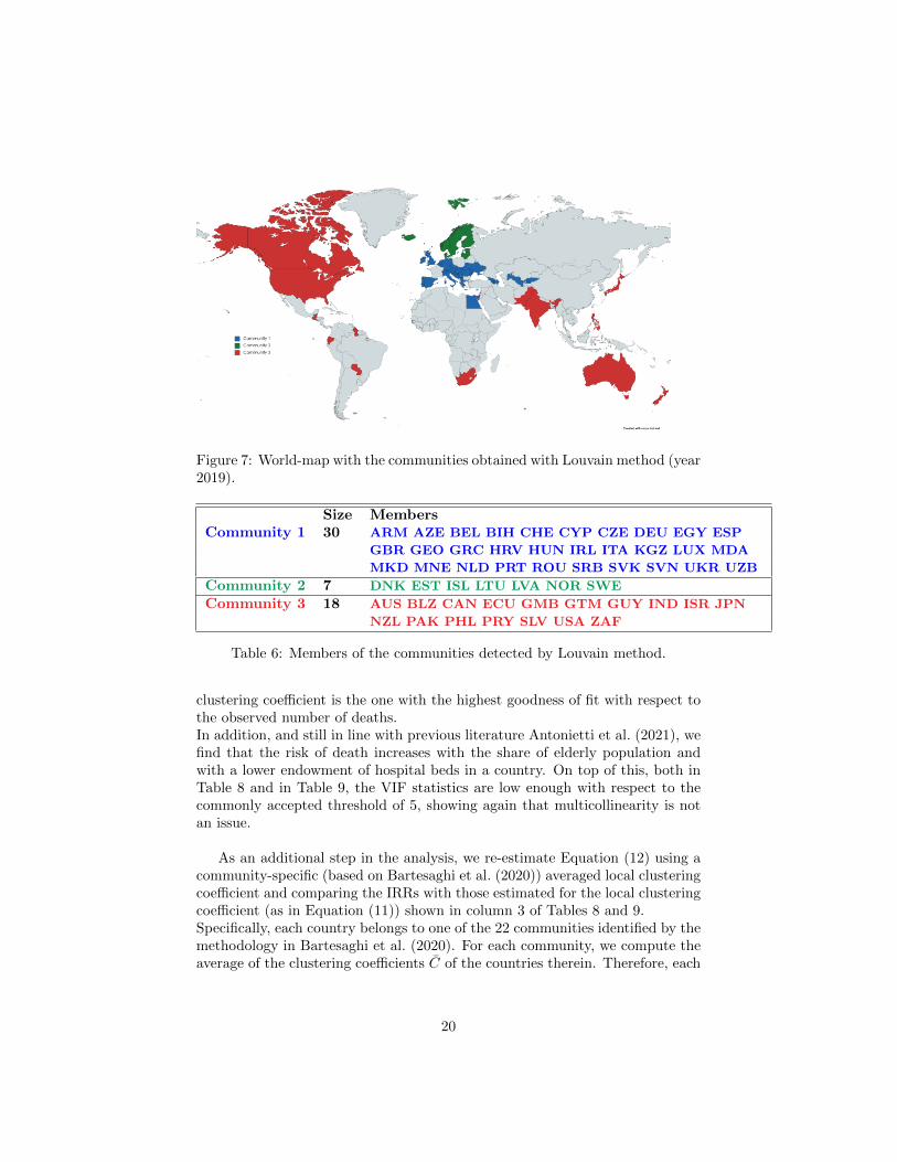
Figure 7: World-map with the communities obtained with Louvain method (year2019).

Size MembersCommunity 1 30 ARM AZE BEL BIH CHE CYP CZE DEU EGY ESP

GBR GEO GRC HRV HUN IRL ITA KGZ LUX MDA

MKD MNE NLD PRT ROU SRB SVK SVN UKR UZB

Community 2 7 DNK EST ISL LTU LVA NOR SWE

Community 3 18 AUS BLZ CAN ECU GMB GTM GUY IND ISR JPN

NZL PAK PHL PRY SLV USA ZAF

Table 6: Members of the communities detected by Louvain method.

clustering coefficient is the one with the highest goodness of fit with respect tothe observed number of deaths.In addition, and still in line with previous literature Antonietti et al. (2021), wefind that the risk of death increases with the share of elderly population andwith a lower endowment of hospital beds in a country. On top of this, both inTable 8 and in Table 9, the VIF statistics are low enough with respect to thecommonly accepted threshold of 5, showing again that multicollinearity is notan issue.

As an additional step in the analysis, we re-estimate Equation (12) using acommunity-specific (based on Bartesaghi et al. (2020)) averaged local clusteringcoefficient and comparing the IRRs with those estimated for the local clusteringcoefficient (as in Equation (11)) shown in column 3 of Tables 8 and 9.Specifically, each country belongs to one of the 22 communities identified by themethodology in Bartesaghi et al. (2020). For each community, we compute theaverage of the clustering coefficients C of the countries therein. Therefore, each

20

Figure 8: World-map with the communities obtained with Louvain method (year2020).

Size MembersCommunity 1 30 ARM AZE BEL BIH CHE CYP CZE DEU EGY ESP

GBR GEO GRC HRV HUN ISL ITA KGZ LUX MDA

MKD MNE NLD PRT ROU SRB SVK SVN UKR UZB

Community 2 7 DNK EST FIN LTU LVA NOR SWE

Community 3 18 AUS BLZ CAN ECU GMB GTM GUY IND IRL ISR

JPN NZL PAK PHL PRY SLV USA ZAF

Table 7: Members of the communities detected by Louvain method in 2020.

country in community k has a new clustering coefficient equal to Ck, defined by

Ck =1

nk

nk∑j=1

Cj (13)

where nk is the size of community k and Ci is the local clustering coefficient ofnode i as in Equation (11).Coefficient C has two properties: on the one hand, it still reflects the country’scentrality within all its triadic relations expressed by the local clustering coeffi-cient in Equation (11). On the other hand, C takes into account the mesoscalestructure of the WTN based on communicability. In other words, with thisnew coefficient, we capture the impact of a country centrality in a subset of theworld trade network, where nodes strongly exchange trade-related informationthat can be directly observable (such as merchandise trade) or indirectly ob-servable (such as the interactions characterizing the supply chain of a good).

Then, we re-estimate Equation (12) using as network centrality measure the

21

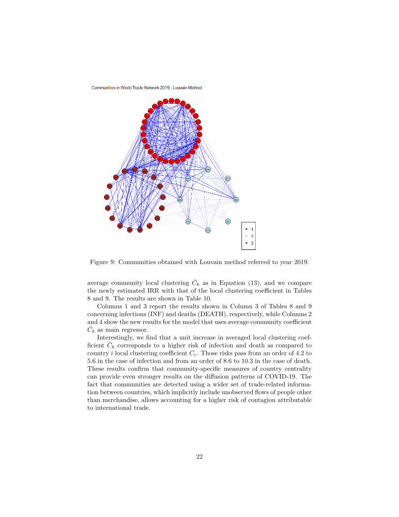
Figure 9: Communities obtained with Louvain method referred to year 2019.

average community local clustering Ck as in Equation (13), and we comparethe newly estimated IRR with that of the local clustering coefficient in Tables8 and 9. The results are shown in Table 10.

Columns 1 and 3 report the results shown in Column 3 of Tables 8 and 9concerning infections (INF) and deaths (DEATH), respectively, while Columns 2and 4 show the new results for the model that uses average community coefficientCk as main regressor.

Interestingly, we find that a unit increase in averaged local clustering coef-ficient Ck corresponds to a higher risk of infection and death as compared tocountry i local clustering coefficient Ci. Those risks pass from an order of 4.2 to5.6 in the case of infection and from an order of 8.6 to 10.3 in the case of death.These results confirm that community-specific measures of country centralitycan provide even stronger results on the diffusion patterns of COVID-19. Thefact that communities are detected using a wider set of trade-related informa-tion between countries, which implicitly include unobserved flows of people otherthan merchandise, allows accounting for a higher risk of contagion attributableto international trade.

22

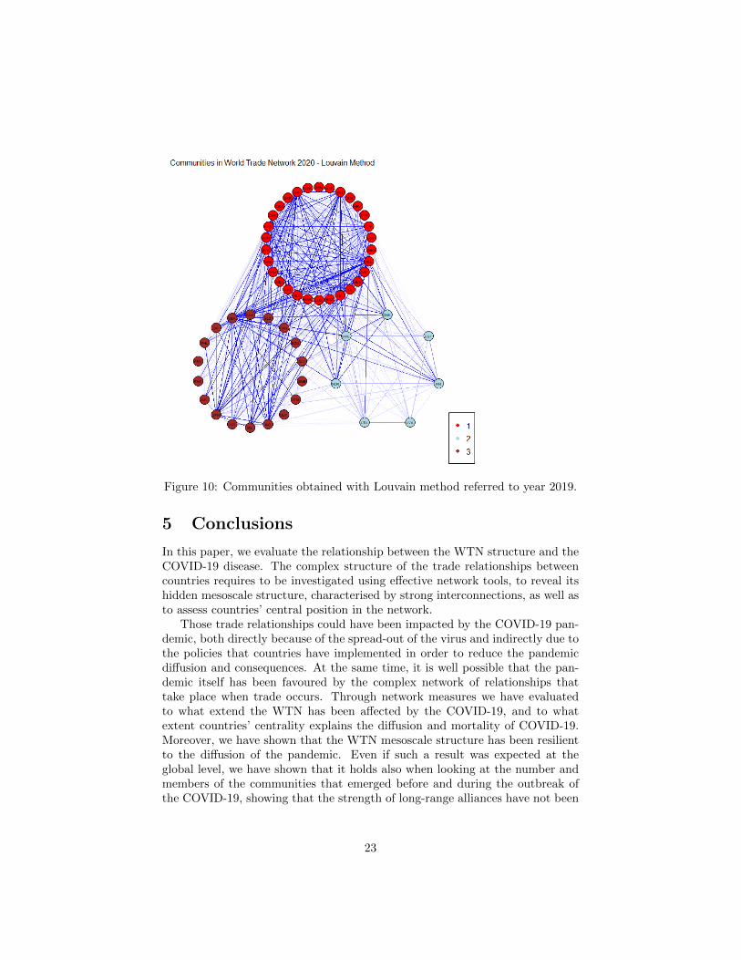
Figure 10: Communities obtained with Louvain method referred to year 2019.

5 Conclusions

In this paper, we evaluate the relationship between the WTN structure and theCOVID-19 disease. The complex structure of the trade relationships betweencountries requires to be investigated using effective network tools, to reveal itshidden mesoscale structure, characterised by strong interconnections, as well asto assess countries’ central position in the network.

Those trade relationships could have been impacted by the COVID-19 pan-demic, both directly because of the spread-out of the virus and indirectly due tothe policies that countries have implemented in order to reduce the pandemicdiffusion and consequences. At the same time, it is well possible that the pan-demic itself has been favoured by the complex network of relationships thattake place when trade occurs. Through network measures we have evaluatedto what extend the WTN has been affected by the COVID-19, and to whatextent countries’ centrality explains the diffusion and mortality of COVID-19.Moreover, we have shown that the WTN mesoscale structure has been resilientto the diffusion of the pandemic. Even if such a result was expected at theglobal level, we have shown that it holds also when looking at the number andmembers of the communities that emerged before and during the outbreak ofthe COVID-19, showing that the strength of long-range alliances have not been

23

affected by the beginning of the COVID-19 pandemic.On the contrary, the country centrality has shown to be a key explanatory vari-able for the diffusion and mortality of COVID-19. We showed that countrycentrality measures strongly explained the risk of infection and mortality, whencontrolling for other possible confounding socio-economic factors.Both results can be of interest for the analysis of the structure and evolutionof the WTN and from the point of view of studying the determinants and theconsequences of the COVID-19 pandemic. Moreover, establishing the link be-tween a pandemic and the structure of the network of international trade canprovide useful policy insights. More precisely, this knowledge can guide deci-sion makers about the adoption and calibration of relevant public safety policies,such as general lockdown measures and temporary trade bans, which have hugeeconomic consequences but have shown so far unclear effectiveness on the virusspread-out. This can be important for both the actual COVID-19 pandemic,which at the time of the writing of this article is still widely diffused worldwide,as well as for the unfortunate yet possible case of the diffusion of a future newpandemic event.

References

Antonietti, R., G. De Masi, and G. Ricchiuti (2020). Linking fdi network topol-ogy with the COVID-19 pandemic. Papers in Evolutionary Economic Geog-raphy n. 20.54 .

Antonietti, R., P. Falbo, and F. Fontini (2021). Assessing the relationshipbetween air quality, wealth, and the first wave of COVID-19 diffusion andmortality. In F. Belaid and S. E. Creti A. (Eds.), Energy Transition, ClimateChange and COVID-19- Economic Impacts. Springer Nature.

Bartesaghi, P., G. P. Clemente, and R. Grassi (2020). Community structurein the world trade network based on communicability distances. Journal ofEconomic Interaction and Coordination, 1–37.

Blochl, F., F. J. Theis, F. Vega-Redondo, and E. O. Fisher (2011). Vertex cen-tralities in input-output networks reveal the structure of modern economies.Physical Review E 83 (4), 046127.

Blondel, V. D., J.-L. Guillaume, R. Lambiotte, and E. Lefebvre (2008). Fastunfolding of communities in large networks. Journal of statistical mechanics:theory and experiment 2008 (10), P10008.

Bonacich, P. (1972). Technique for analyzing overlapping memberships. Socio-logical methodology 4, 176–185.

Bontempi, E. and M. Coccia (2021). International trade as critical parameterof COVID-19 spread that outclasses demographic, economic, environmental,and pollution factors. Environmental Research, 111514.

24

Bontempi, E., M. Coccia, S. Vergalli, and A. Zanoletti (2021). Can commercialtrade represent the main indicator of the COVID-19 diffusion due to human-to-human interactions? a comparative analysis between italy, france, andspain. Environmental Research, 111529.

Chang, C., W. Liao, Y. Chen, and L. Liou (2016). A mathematical theoryfor clustering in metric spaces. IEEE Transactions on Network Science andEngineering 3 (1), 2–16.

Crofts, J. J. and D. J. Higham (2009). A weighted communicability measure ap-plied to complex brain networks. Journal of the Royal Society Interface 6 (33),411–414.

De Benedictis, L. and L. Tajoli (2011). The world trade network. The WorldEconomy 34 (8), 1417–1454.

Estrada, E. (2012, Jun). Complex networks in the euclidean space of commu-nicability distances. Phys. Rev. E 85, 066122.

Estrada, E. and N. Hatano (2008, Mar). Communicability in complex networks.Phys. Rev. E 77, 036111.

Estrada, E. and N. Hatano (2009, August). Communicability graph and commu-nity structures in complex networks. Appl. Math. Comput. 214 (2), 500–511.

Estrada, E. and J. A. Rodriguez-Velazquez (2005, 06). Subgraph centrality incomplex networks. Physical review. E, Statistical, nonlinear, and soft matterphysics 71, 056103.

Fagiolo, G. (2020). Assessing the impact of social network structure on the dif-fusion of coronavirus disease (COVID-19): A generalized spatial seird model.arXiv preprint arXiv:2010.11212 .

Fagiolo, G., J. Reyes, and S. Schiavo (2010). The evolution of the world tradeweb: a weighted-network analysis. Journal of Evolutionary Economics 20 (4),479–514.

Fernandez-Villaverde, J. and C. I. Jones (2020). Macroeconomic outcomes andCOVID-19: a progress report. Technical report, National Bureau of EconomicResearch.

Fortunato, S. and D. Hric (2016). Community detection in networks: A userguide. Physics reports 659, 1–44.

Grassi, R., P. Bartesaghi, S. Benati, and G. P. Clemente (2021). Multi-attributecommunity detection in international trade network. Networks and SpatialEconomics, 1–27.

Horn, R. A. and C. R. Johnson (2012). Matrix analysis. Cambridge universitypress.

25

James, G., D. Witten, T. Hastie, and R. Tibshirani (2013). An introduction tostatistical learning, Volume 112. Springer.

Kali, R. and J. Reyes (2007). The architecture of globalization: a network ap-proach to international economic integration. Journal of International Busi-ness Studies 38 (4), 595–620.

Kiyota, K. (2021). The COVID-19 pandemic and the world trade network.

Newman, M. E. (2001). Clustering and preferential attachment in growingnetworks. Physical review E 64 (2), 025102.

Onnela, J., J. Saramaki, J. Kertesz, and K. Kaski (2005, jun). Intensity andcoherence of motifs in weighted complex networks. Physical Review E 71 (6).

Paez, A., F. A. Lopez, T. Menezes, R. Cavalcanti, and M. G. d. R. Pitta (2020).A spatio-temporal analysis of the environmental correlates of COVID-19 in-cidence in spain. Geographical analysis.

Parodi, E. and S. Aloisi (2020). Italian scientists investigate possible earlieremergence of coronavirus.

Piccardi, C. and L. Tajoli (2018, 11). Complexity, centralization, and fragilityin economic networks. PLOS ONE 13 (11), 1–13.

Reissl, S., A. Caiani, F. Lamperti, M. Guerini, F. Vanni, G. Fagiolo, T. Ferraresi,L. Ghezzi, M. Napoletano, and A. Roventini (2021). Assessing the economiceffects of lockdowns in italy: a dynamic input-output approach.

Russo, L., C. Anastassopoulou, A. Tsakris, G. N. Bifulco, E. F. Campana,G. Toraldo, and C. Siettos (2020). Tracing day-zero and forecasting theCOVID-19 outbreak in lombardy, italy: A compartmental modelling and nu-merical optimization approach. Plos one 15 (10), e0240649.

Sabidussi, G. (1966). The centrality index of a graph. Psychometrika 31 (3),581–603.

Serrano, M. A., M. Boguna, and A. Vespignani (2007). Patterns of dominantflows in the World trade web. Journal of Economic Interaction and Coordi-nation 2 (2), 111–124.

The European Centre for Disease Prevention and Control (2021). Dataon the daily number of new reported COVID-19 cases and deaths byeu/eea country. data retrieved from European Center for Disease Preven-tion and Control, https://www.ecdc.europa.eu/en/publications-data/

data-daily-new-cases-COVID-19-eueea-country.

The World Bank (2021). World development indicators. data retrievedfrom World Development Indicators, https://databank.worldbank.org/

source/world-development-indicators.

26

Tzekina, I., K. Danthi, and D. N. Rockmore (2008). Evolution of communitystructure in the world trade web. The European Physical Journal B 63 (4),541–545.

Un Comtrade (2021). International trade statistics database. data retrievedfrom International Trade Statistics Database, https://comtrade.un.org/.

A Table of countries

27

DEP. VAR.: INF (1) (2) (3) (4) (5)Degree 3.608***

(0.631)Betweenness 4.121***

(1.868)Local Clustering 4.201***

(0.968)Weighted Eigenvector 3.225***

(0.875)Strength (:109) 3.339***

(1.052)GDPPC 1.676 1.147 1.191** 1.238* 1.264**

(0.632) (0.266) (0.103) (0.144) (0.133)POP 3.026 1.813 1.023 1.132 1.136

(3.227) (2.130) (0.134) (0.224) (0.184)POP65+ 2.226*** 1.685 1.688*** 2.680*** 2.420***

(0.685) (0.539) (0.294) (0.636) (0.564)HBEDS 0.678 0.710 0.585*** 0.557** 0.555***

(0.212) (0.230) (0.087) (0.132) (0.107)TEMP 1.120 0.728 1.080 1.387 1.316

(0.226) (0.335) (0.142) (0.350) (0.231)Week dummies yes yes yes yes yesOverdispersion (α) 1.319*** 1.393*** 0.998*** 1.263*** 1.193***

(0.209) (0.170) (0.178) (0.213) (0.204)N 275 275 275 275 275Log Pseudo-likelihood -2490.6 -2500.5 -2440.5 -2482.5 -2472.2AIC 5005.1 5025.1 4905.1 4989.0 4968.4BIC 5048.5 5068.5 4948.4 5032.4 5011.82Pseudo R2 0.076 0.072 0.094 0.079 0.083Max VIF 3.01 3.20 2.72 2.57 2.60Mean VIF 1.79 1.89 1.73 1.69 1.68

Country-level clustered standard errors in parentheses.All the estimates also include a constant term. * p < 0.1, ** p < 0.05, *** p < 0.01.

Table 8: Negative binomial regressions: infections, incidence rate ratios

28

DEP. VAR.: DEATH (1) (2) (3) (4) (5)Degree 2.878***

(0.888)Betweenness 6.750***

(3.022)Local Clustering 8.648***

(3.579)Weighted Eigenvector 5.123**

(3.339)Strength (:109) 6.893***

(5.123)GDPPC 1.458 0.755 0.930 0.933 0.966

(0.671) (0.162) (0.141) (0.149) (0.136)POP 2.897 1.486 0.867 1.020 1.016

(3.258) (1.636) (0.102) (0.196) (0.169)POP65+ 6.223*** 3.099*** 2.136*** 5.423*** 4.037***

(2.549) (1.216) (0.606) (2.338) (1.830)HBEDS 0.370*** 0.434*** 0.484*** 0.382*** 0.429***

(0.105) (0.127) (0.099) (0.119) (0.127)TEMP 1.721 0.973 1.426* 1.968 1.915**

(0.471) (0.424) (0.272) (0.814) (0.556)Week dummies yes yes yes yes yesOverdispersion (α) 2.245*** 2.055*** 1.400*** 1.933*** 1.805***

(0.283) (0.255) (0.217) (0.266) (0.263)N 275 275 275 275 275Log Pseudo-likelihood -1519.4 -1500.6 -1437.9 - 1490.9 -1479.2AIC 3062.9 3025.3 2899.9 3005.7 2982.3BIC 3106.3 3068.7 2943.3 3049.2 3025.7Pseudo R2 0.101 0.112 0.149 0.118 0.124Max VIF 3.01 3.20 2.72 2.57 2.60Mean VIF 1.79 1.89 1.73 1.69 1.68

Country-level clustered standard errors in parentheses.All the estimates also include a constant term. * p < 0.1, ** p < 0.05, *** p < 0.01.

Table 9: Negative binomial regressions: deaths, incidence rate ratios

29

DEP. VAR.: INF DEATH

(1) (2) (3) (4)Local Clustering 4.201*** 8.648***

(0.968) (3.579)Average Community Clustering 5.551*** 10.25***

(2.486) (4.977)bGDPPC 1.191** 1.510** 0.930 1.166

(0.103) (0.243) (0.141) (0.199)POP 1.023 2.499 0.867 2.107

(0.134) (2.467) (0.102) (2.137)POP65+ 1.688*** 1.705** 2.136*** 2.945***

(0.294) (0.425) (0.606) (0.904)HBEDS 0.585*** 0.652* 0.484*** 0.419***

(0.087) (0.146) (0.099) (0.087)TEMP 1.080 0.980 1.426* 1.294

(0.142) (0.286) (0.272) (0.448)Week dummies yes yes yes yesOverdispersion (α) 0.998*** 1.344*** 1.400*** 1.898***

(0.178) (0.211) (0.217) (0.284)N 275 275 275 275Pseudo R2 0.094 0.074 0.149 0.120

Country-level clustered standard errors in parentheses.All the estimates also include a constant term.* p < 0.1, ** p < 0.05, *** p < 0.01.

Table 10: General vs average community clustering coefficient and COVID-19diffusion.

30

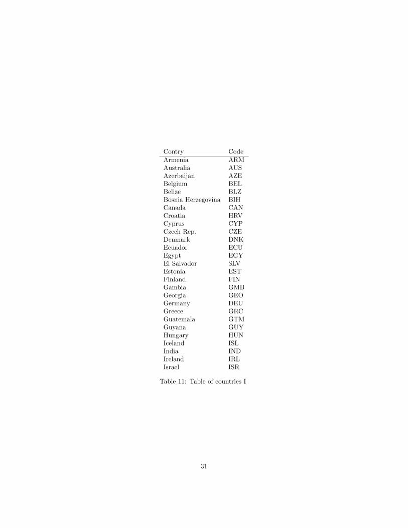
Contry CodeArmenia ARMAustralia AUSAzerbaijan AZEBelgium BELBelize BLZBosnia Herzegovina BIHCanada CANCroatia HRVCyprus CYPCzech Rep. CZEDenmark DNKEcuador ECUEgypt EGYEl Salvador SLVEstonia ESTFinland FINGambia GMBGeorgia GEOGermany DEUGreece GRCGuatemala GTMGuyana GUYHungary HUNIceland ISLIndia INDIreland IRLIsrael ISR

Table 11: Table of countries I

31

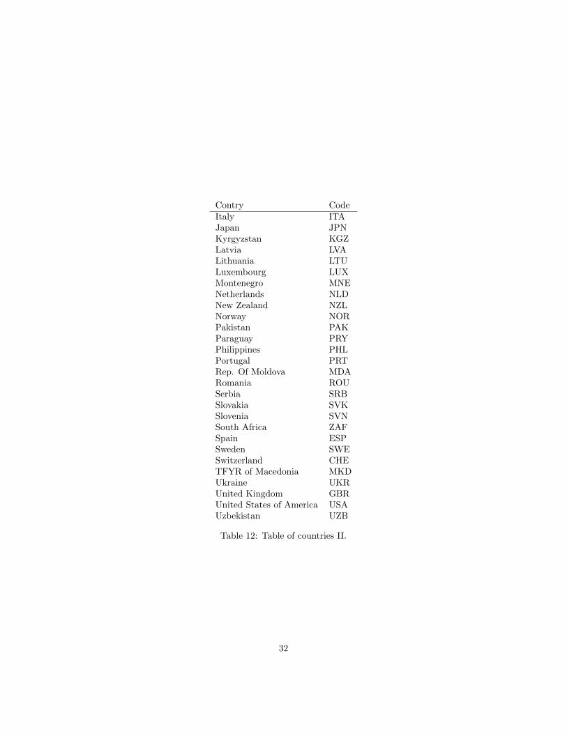
Contry CodeItaly ITAJapan JPNKyrgyzstan KGZLatvia LVALithuania LTULuxembourg LUXMontenegro MNENetherlands NLDNew Zealand NZLNorway NORPakistan PAKParaguay PRYPhilippines PHLPortugal PRTRep. Of Moldova MDARomania ROUSerbia SRBSlovakia SVKSlovenia SVNSouth Africa ZAFSpain ESPSweden SWESwitzerland CHETFYR of Macedonia MKDUkraine UKRUnited Kingdom GBRUnited States of America USAUzbekistan UZB

Table 12: Table of countries II.

32