International Series in Operations Research& Management Science

Volume 127

Series Editor

Frederick S. HillierStanford University, CA, USA

INT. SERIES IN OPERATIONS RESEARCH & MANAGEMENT SCIENCESeries Editor: Frederick S. Hillier, Stanford University

Special Editorial Consultant: Camille C. Price, Stephen F. Austin State UniversityTitles with an asterisk (*) were recommended by Dr. Price

Axsäter/ INVENTORY CONTROL, 2ndEd.Hall/ PATIENT FLOW: Reducing Delay in Healthcare DeliveryJózefowska & Weglarz/ PERSPECTIVES IN MODERN PROJECT SCHEDULINGTian & Zhang/ VACATION QUEUEING MODELS: Theory and ApplicationsYan, Yin & Zhang/ STOCHASTIC PROCESSES, OPTIMIZATION, AND CONTROL THEORY

APPLICATIONS IN FINANCIAL ENGINEERING, QUEUEING NETWORKS, ANDMANUFACTURING SYSTEMS

Saaty & Vargas/ DECISION MAKING WITH THE ANALYTIC NETWORK PROCESS: Economic, Political,Social & Technological Applications w. Benefits, Opportunities, Costs & Risks

Yu/ TECHNOLOGY PORTFOLIO PLANNING AND MANAGEMENT: Practical Concepts and ToolsKandiller/ PRINCIPLES OF MATHEMATICS IN OPERATIONS RESEARCHLee & Lee/ BUILDING SUPPLY CHAIN EXCELLENCE IN EMERGING ECONOMIESWeintraub/ MANAGEMENT OF NATURAL RESOURCES: A Handbook of Operations Research Models,

Algorithms, and ImplementationsHooker/ INTEGRATED METHODS FOR OPTIMIZATIONDawande et al/ THROUGHPUT OPTIMIZATION IN ROBOTIC CELLSFriesz/ NETWORK SCIENCE, NONLINEAR SCIENCE and INFRASTRUCTURE SYSTEMSCai, Sha & Wong/ TIME-VARYING NETWORK OPTIMIZATIONMamon & Elliott/ HIDDEN MARKOV MODELS IN FINANCEdel Castillo/ PROCESS OPTIMIZATION: A Statistical ApproachJózefowska/JUST-IN-TIME SCHEDULING: Models & Algorithms for Computer & Manufacturing SystemsYu, Wang & Lai/ FOREIGN-EXCHANGE-RATE FORECASTING WITH ARTIFICIAL NEURAL NETWORKSBeyer et al/ MARKOVIAN DEMAND INVENTORY MODELSShi & Olafsson/ NESTED PARTITIONS OPTIMIZATION: Methodology and ApplicationsSamaniego/ SYSTEM SIGNATURES AND THEIR APPLICATIONS IN ENGINEERING RELIABILITYKleijnen/DESIGN AND ANALYSIS OF SIMULATION EXPERIMENTSFørsund/ HYDROPOWER ECONOMICSKogan & Tapiero/ SUPPLY CHAIN GAMES: Operations Management and Risk ValuationVanderbei/ LINEAR PROGRAMMING: Foundations & Extensions, 3rd EditionChhajed & Lowe/BUILDING INTUITION: Insights from Basic Operations Mgmt. Models and PrinciplesLuenberger & Ye/LINEAR AND NONLINEAR PROGRAMMING, 3rd EditionDrew et al/ COMPUTATIONAL PROBABILITY: Algorithms and Applications in the Mathematical Sciences*Chinneck/ FEASIBILITY AND INFEASIBILITY IN OPTIMIZATION: Algorithms and Computation MethodsTang, Teo & Wei/ SUPPLY CHAIN ANALYSIS: A Handbook on the Interaction of Information, System and

OptimizationOzcan/ HEALTH CARE BENCHMARKING AND PERFORMANCE EVALUATION: An Assessment using

Data Envelopment Analysis (DEA)Wierenga/ HANDBOOK OF MARKETING DECISION MODELSAgrawal & Smith/ RETAIL SUPPLY CHAIN MANAGEMENT: Quantitative Models and Empirical StudiesBrill/ LEVEL CROSSING METHODS IN STOCHASTIC MODELSZsidisin & Ritchie/ SUPPLY CHAIN RISK: A Handbook of Assessment, Management & PerformanceMatsui/ MANUFACTURING AND SERVICE ENTERPRISE WITH RISKS: A Stochastic Management ApproachZhu/ QUANTITATIVE MODELS FOR PERFORMANCE EVALUATION AND BENCHMARKING: Data

Envelopment Analysis with Spreadsheets

∼A list of the early publications in the series is found at the end of the book∼

Wieslaw Kubiak

Proportional Optimizationand Fairness

123

Wieslaw KubiakMemorial UniversityFaculty AdministrationJohn’s NLCanada A1B 3X5wkubiak@mun.ca

ISBN: 978-0-387-87718-1 e-ISBN: 978-0-387-87719-8DOI: 10.1007/978-0-387-87719-8

Library of Congress Control Number: 2008934787

c© Springer Science+Business Media, LLC 2009All rights reserved. This work may not be translated or copied in whole or in part without the writtenpermission of the publisher (Springer Science+Business Media, LLC, 233 Spring Street, New York,NY 10013, USA), except for brief excerpts in connection with reviews or scholarly analysis. Use inconnection with any form of information storage and retrieval, electronic adaptation, computer software,or by similar or dissimilar methodology now known or hereafter developed is forbidden.The use in this publication of trade names, trademarks, service marks, and similar terms, even if they arenot identified as such, is not to be taken as an expression of opinion as to whether or not they are subjectto proprietary rights.

Printed on acid-free paper

springer.com

of

To My Inka i Michał

Preface

If the beginning provides countless possibilities, then why not to start with fewquestions? Why are cars of different colors spread along an assembly line rather thenbatched together in a single long sequence of the same color? How to make equalpriority jobs progress at the rates proportional to their lengths so that a job twice thelength of another one gets a shared resource allocated twice the time of the other jobup to any point in time? Or a client who pays three times more for its computationsthan another client gets its computations to progress three times faster than the otherclient’s by getting more processor and bandwidth allocations? How to make surethat the Internet gateway bandwidth is shared fairly so that the community sharingthe network is not reduced to few getting all and most nothing? All these questionsdeal with proportional representation either according to the demand for particularcar color, or according to the job length or its right to resources, or according to thereciprocal of the packet size to name just few. They are fundamental even more sotoday when we are surrounded by systems enabled by technology to work in a just-in-time mode since this mode very principle requires a steady, smooth, and evenlyspread progress of tasks in time. The progress is proportional to the demand for thetasks’s outcomes.

As a thinker and futurist Alvin Toffler [1] in his Financial Times interview pointsout “Global positioning satellites are key to synchronising precision time and datastreams for everything from mobile phone calls to ATM withdrawals. They allowjust-in-time productivity because of precise tracking.”

What is somewhat surprising is that all these questions that seem so far aparthave similar underlying framework, which is simply speaking to build a finite orinfinite often cyclic sequence; we shall refer to it as a just-in-time sequence, ona finite n letter alphabet where each letter is spread “as evenly as possible” andoccurs with a given rate or a given number of times. The problem of finding such asequence is not only a mathematical one since there is no mathematical definitionof “as evenly as possible” that would satisfactorily capture the challenge behindthis phrase. The problem can find many mathematical formulations, but none willprobably satisfy all. Thus, one way of approaching the problem is to use the well-known apportionment theory and especially its house monotone methods to buildthe desired just-in-time sequence.

vii

viii Preface

The apportionment problem has its roots in the proportional representation sys-tem designed for the House of Representatives of the United States where each statereceives seats in the House proportionally to its population. The theory has been inthe making for more than 200 years now and its exciting story as well as main resultscan be found in an excellent book by Balinski and Young [2], see also more recentbook by Young [3], and Balinski’s popular introduction in [4]. The title of Balinskiand Young’s book speaks for itself: “Fair Representation: Meeting the Ideal of OneMan, One Vote.” Its main underlying message is that the ideal is not one but manyand that we can only hope to agree on one by stating some “obvious” axioms thatit must meet and then find a method that would deliver a solution meeting theseaxioms, or to prove that one does not exist. This process may, however, not save usfrom falling into various anomalies that do not contradict the axioms yet may be atodds with the commonly accepted sense of fair representation.

This book argues that the apportionment methods, in particular the John QuincyAdams’s and the Thomas Jefferson’s, have been widely, yet unknowingly, rediscov-ered and used in resource allocation and sequencing computer, manufacturing, andother real-life technical systems. Sometimes without a clear understanding of whatsolutions they lead to in terms of their properties. The properties which have beenwell researched and known from the apportionment literature but missing in thetechnical one, either computer science or operations research. This lack of propercontext may have resulted, as we argue in some parts of this book, in overlookingother apportionment methods, in particular the Daniel Webster’s method, that mayoffer a number of additional attractive properties, like being better balanced thaneither the Adams’s or the Jefferson’s.

The axiomatic approach favored by the apportionment theory for the proportionalrepresentation systems is preferred over an optimization approach championed byoperations research scientists since the problem with the latter approach is in thewords of Balinski and Young from [2] as follows: “The moral of this tale is thatone cannot choose objective functions with impunity, despite current practices inapplied mathematics. The choice of an objective is, by and large an ad hoc affair. . .Of much deeper significance than the formulas that are used are the properties theyenjoy.”

We think, however, that in order to adequately address the proportional represen-tation problems listed at the beginning of this preface and others we need to studythem not only through the apportionment theory but through optimization as well.After all the questions of quantifying excess inventory and shortage in just-in-timemanufacturing, the throughput error in stride scheduling, or the relative and absolutebounds in fair queueing are clearly important. By doing so, we also realize that theoptimization reveals a new role of the well-known apportionment methods, the Web-ster’s method in particular. The optimization moreover reveals connections with thewell-known and still open mathematical conjectures as the Fraenkel’s Conjecture,see Tijdeman [5] for a brief account and Chap. 6, finally it relates to the multimodu-lar functions minimization, introduced by Hajek [6] and later developed by Altmanet al. [7], which aims at evenly spreading the demand and workload in computer andsupply chains.

Preface ix

The question of which objective function to choose we settle by choosing eithertotal deviation or maximum deviation objective functions. Our solution method isgeneral enough to include a large class of point deviation functions. The choice ofobjective functions follows sometime the choice made by Monden who, in his sem-inal book [8], described the Goal Chasing Method of Toyota by using the squarepoint deviation function which apparently follows the minimization of square errorin the least squares method of Carl Friedrich Gauss. The attractive feature of this op-timization is that it can be done efficiently, though certain intriguing computationalcomplexity issues remain open, and produce solutions which have many though notall, by the Impossibility Theorem of Balinski and Young [2], desirable propertiesidentified by the theory and practice of apportionment.

The book intends to chart a solid common ground for discussing and solvingproblems ranging from sequencing mixed-model just-in-time assembly lines,through just-in-time batch production, balancing workloads in event graphs tobandwidth allocation in the Internet gateways and resource allocation in operatingsystems. From problems in mathematics of social sciences through operations re-search and computer science problems, it argues that the apportionment theory andthe optimization based on deviation functions provide natural benchmarks in thisprocess. However, the process has just started and this book is to provide just asmall stepping stone on the way to this common ground. Needless to say it will bea great pleasure for the author if the book’s topic finds its followers.

The book includes mostly very recent results – some of them published recently,some of them new and yet unpublished. It includes ten main chapters. Chapter 2briefly reviews main results of the apportionment theory used in the remainder ofthe book. It emphasizes the axiomatic approach to the apportionment problem andto the construction of the just-in-time sequences. The approach relies on the divisormethods, in particular parametric methods advocated by Balinski and Young [2],and their desirable properties embedded in the resulting just-in-time sequences.Chapter 3 considers the problems of deviation minimization, the total and the max-imum deviation, as tools for obtaining just-in-time sequences. It formulates theseproblems as nonlinear integer optimization and presents efficient algorithms fortheir solution. The algorithms are based on the concept of ideal positions, closelyrelated to the Webster’s apportionment method. They transform the deviation min-imization problems to either the assignment or the bottleneck assignment problem,respectively, and then solve the latter. The algorithms run in time which is polyno-mial in the length of the outcome just-in-time output sequence. Chapter 4 proves thatthere exist cyclic solutions that minimize the total deviation for symmetric point de-viation functions, the same is shown for the maximum deviation. It also proves thatlimiting optimization to the sequences with the bottleneck deviation not exceeding1 renders some functions of point deviation equivalent. The oneness property claimsthat limiting search for optimal just-in-time sequences to those with bottleneck notexceeding 1 will be optimal in general. However, the chapter shows that all opti-mal just-in-time sequences for some instances may have the bottleneck deviationhigher than 1 – thus showing that the oneness does not hold generally. Chapter 5gives a more efficient algorithm for the maximum absolute deviation (referred to

x Preface

as bottleneck) deviation. The absolute value function of deviation results in optimalbottleneck being always less than 1, and allows to develop strong upper and lowerbounds on the optimal bottleneck. These bounds and other properties of the bottle-neck optimal just-in-time sequences are used in the application to the Liu–Laylandproblem, stride scheduling, fair queueing, and others in the subsequent chapters.Chapter 5 also shows that the optimal bottleneck just-in-time sequences for n = 2are in fact Webster’s sequences of apportionment and the most regular words atthe same time; thus, they optimize the throughput of any two cyclic process shar-ing a common resource. This new observation underlines again the advantages ofthe Webster’s sequences for other than apportionment problems. Chapter 6 furtherexploits the properties of just-in-time sequences with small bottleneck deviations,which are understood as those less than 1

2 . The question is what are the instancesthat admit this small bottleneck deviation? The answer given in the chapter is thatthere is only one, called the power-of-two instance that results in this small bot-tleneck deviation for n ≥ 3. The chapter also shows the connection between thesmall bottleneck deviation problem and the famous Fraenkel’s Conjecture, whichstates that the only distinct rates for which it is possible to build a balanced wordon three or more letters come essentially from the power-of-two instances. Finally,the chapter presents the small bottleneck problem in the broader context of regularsequences and multimodular functions they minimize. The applications of multi-modular functions to workload balancing in event graphs (for instance the queuesand supply chains) are also discussed in the chapter. Chapter 7 addresses the re-sponse time variability minimization problem, where the average response time fora client is a reciprocal of its desirable rate. Thus, being as close as possible to theaverage response time aims at achieving the “as evenly as possible” goal. The re-sponse time variability is one of the main objectives in stride scheduling as well. Thechapter shows that the problem is NP-hard, proposes exact and heuristic solutions,and reports computational experiments with the latter. Chapter 8 proves that theoptimal bottleneck sequences make tasks progress at the rates close enough to thetasks’ processing time to request interval ratios so that they solve the Liu–Laylandproblem – likely the best known scheduling problem in the hard real-time systems.It also gives necessary conditions for the apportionment divisor methods to solvethe Liu–Layland problem, and proves that the quota-divisor methods solve the Liu–Layland problem as well. Finally, the chapter presents solutions to some specialcases of the pinwheel scheduling problem given by the bottleneck optimal just-in-time sequences. Chapter 9 focuses on the problem of constructing just-in-timesequences for supply chains so that the temporal capacity constraints imposed bysuppliers are respected. The constraints are modeled by giving the limiting, supply-dependent proportions p: q that stipulate that at most p out of any q models deliveredby the supply chain must be supplied by a particular supplier. Though the problemof finding such a sequence is NP-hard in the strong sense the chapter discusses anumber of approaches: synchronized delivery and periodic synchronized deliveryfor better balancing workloads in supply chains. Finally, the chapter points out a po-tential for using tools developed by the combinatorics on words to design the just-in-time sequences having desirable properties, and discusses the class of balanced

Preface xi

words in this role in more detail. Chapter 10 looks into the problem of fairness in fairqueueing and stride scheduling. It shows that both use the Jefferson’s and Adams’smethod of apportionment, and both are peer-to-peer fair. However, the chapter alsoargues that the Webster’s method could prove a better yet untested choice for fairqueueing and stride scheduling. The chapter gives also a closer look at the measuresand criteria typically used in the fair queueing and stride scheduling and analyzesthem using the apportionment theory and just-in-time optimization tools developedin Chaps. 2, 5, and 7. Finally, Chap. 11 extends the models developed in Chaps. 2,3, and 9 to manufacturing environments with variable processing and set-up times.This is a departure from the usual assumption of negligible variability resulting in ansimplification, often criticized, of unit times and synchronized lines assumed in theapplications of just-in-time sequences. The chapter’s approach is based on batchingto smooth out the variability of processing and set-up times, and then on sequencingthe batches to minimize the total deviation or alternatively to gain the advantages ofthe Webster’s method. The approach is applied to a real-life problem arising in anautomotive pressure hose manufacturer. The computational experiments with bothalgorithms are also presented in the chapter.

Special thanks go to my friends and colleagues, listed here in a random order, fortheir encouragement and support: Prof. Dominique de Werra (Ecole PolitechniqueFederale de Lausanne), Profs. Jan Weglarz and Jacek Błazewicz (Poznan Universityof Technology), Prof. Albert Corominas (Universitat Politecnica de Catalunya),Prof. Jacques Cariler (Universite de Technologie de Compiegne), Prof. Erwin Pesch(University of Siegen), Prof. Moshe Dror (University of Arizona), Prof. Gerd Finke(Universite Joseph Fourier), and Prof. Marek Kubale (Gdansk University of Tech-nology). I am indebted in particular to Dr. Cynthia Philips (Sandia National Labo-ratories) and Dr. Bruno Gaujal (INRIA-Grenoble) for pointing me to a number ofimportant references.

Finally, I wish to acknowledge the research support of the Natural Sciencesand Engineering Research Council of Canada without which many of my researchprojects on just-in-time would simply not happen.

St. John’s, Canada Wieslaw Kubiak

Contents

1 Preliminaries . . . . . . . . . . . . . . . . . . . . . . . . . . . . . . . . . . . . . . . . . . . . . . . . . . 1

2 The Theory of Apportionment and Just-In-Time Sequences . . . . . . . . . 52.1 Introduction . . . . . . . . . . . . . . . . . . . . . . . . . . . . . . . . . . . . . . . . . . . . . . . 52.2 The Apportionment Problem . . . . . . . . . . . . . . . . . . . . . . . . . . . . . . . . . 62.3 Which Apportionment? . . . . . . . . . . . . . . . . . . . . . . . . . . . . . . . . . . . . . 7

2.3.1 The Basics: Exact, Anonymous and HomogeneousApportionments . . . . . . . . . . . . . . . . . . . . . . . . . . . . . . . . . . . . . 7

2.3.2 House Monotone Apportionments . . . . . . . . . . . . . . . . . . . . . . 82.3.3 Population Monotone Apportionments . . . . . . . . . . . . . . . . . . 92.3.4 Uniform Apportionments . . . . . . . . . . . . . . . . . . . . . . . . . . . . . 92.3.5 Apportionments Satisfying Quota . . . . . . . . . . . . . . . . . . . . . . 10

2.4 Apportionment Methods . . . . . . . . . . . . . . . . . . . . . . . . . . . . . . . . . . . . . 102.4.1 Divisor Methods . . . . . . . . . . . . . . . . . . . . . . . . . . . . . . . . . . . . . 102.4.2 Parametric Methods . . . . . . . . . . . . . . . . . . . . . . . . . . . . . . . . . . 132.4.3 Rank-Index Methods . . . . . . . . . . . . . . . . . . . . . . . . . . . . . . . . . 13

2.5 What is Impossible? . . . . . . . . . . . . . . . . . . . . . . . . . . . . . . . . . . . . . . . . 142.6 Coalitions and Schisms . . . . . . . . . . . . . . . . . . . . . . . . . . . . . . . . . . . . . . 182.7 From Apportionments to Just-In-Time Sequences . . . . . . . . . . . . . . . . 202.8 Which Just-In-Time Apportionments? . . . . . . . . . . . . . . . . . . . . . . . . . 21

2.8.1 Cycles . . . . . . . . . . . . . . . . . . . . . . . . . . . . . . . . . . . . . . . . . . . . . 212.8.2 Advancing and Delaying . . . . . . . . . . . . . . . . . . . . . . . . . . . . . . 232.8.3 Symmetry and Quasi-Palindromes . . . . . . . . . . . . . . . . . . . . . . 25

2.9 The Consistency of Webster’s Method . . . . . . . . . . . . . . . . . . . . . . . . . 272.10 Exercises . . . . . . . . . . . . . . . . . . . . . . . . . . . . . . . . . . . . . . . . . . . . . . . . . 302.11 Comments and References . . . . . . . . . . . . . . . . . . . . . . . . . . . . . . . . . . . 31

3 Minimization of Just-In-Time Sequence Deviation . . . . . . . . . . . . . . . . . 333.1 Introduction . . . . . . . . . . . . . . . . . . . . . . . . . . . . . . . . . . . . . . . . . . . . . . . 333.2 Minimization of Total Deviation . . . . . . . . . . . . . . . . . . . . . . . . . . . . . . 343.3 The Transformation to the Assignment Problem . . . . . . . . . . . . . . . . . 35

xiii

xiv Contents

3.4 The Monge Property of Assignment Costs . . . . . . . . . . . . . . . . . . . . . . 413.5 The Equivalence . . . . . . . . . . . . . . . . . . . . . . . . . . . . . . . . . . . . . . . . . . . 463.6 The Solution . . . . . . . . . . . . . . . . . . . . . . . . . . . . . . . . . . . . . . . . . . . . . . 483.7 Minimization of Maximum Deviation . . . . . . . . . . . . . . . . . . . . . . . . . 503.8 The Bottleneck Assignment . . . . . . . . . . . . . . . . . . . . . . . . . . . . . . . . . . 503.9 The Bottleneck Monge Property . . . . . . . . . . . . . . . . . . . . . . . . . . . . . . 523.10 Exercises . . . . . . . . . . . . . . . . . . . . . . . . . . . . . . . . . . . . . . . . . . . . . . . . . 533.11 Comments and References . . . . . . . . . . . . . . . . . . . . . . . . . . . . . . . . . . . 54

4 Optimality of Cyclic Sequences and the Oneness . . . . . . . . . . . . . . . . . . . 554.1 Introduction . . . . . . . . . . . . . . . . . . . . . . . . . . . . . . . . . . . . . . . . . . . . . . . 554.2 Symmetries of Ci

jks for Symmetric Fis . . . . . . . . . . . . . . . . . . . . . . . . . 574.3 The Folding, Shuffling, and Unfolding of Sequences . . . . . . . . . . . . . 65

4.3.1 The Folding . . . . . . . . . . . . . . . . . . . . . . . . . . . . . . . . . . . . . . . . . 684.3.2 The Shuffling . . . . . . . . . . . . . . . . . . . . . . . . . . . . . . . . . . . . . . . 684.3.3 The Unfolding . . . . . . . . . . . . . . . . . . . . . . . . . . . . . . . . . . . . . . . 694.3.4 Folding, Shuffling and Unfolding Yield An Assignment . . . . 69

4.4 Optimality of Cyclic Solutions for Total Deviation . . . . . . . . . . . . . . . 714.5 Optimality of Cyclic Solutions for Maximum Deviation . . . . . . . . . . 724.6 The Oneness . . . . . . . . . . . . . . . . . . . . . . . . . . . . . . . . . . . . . . . . . . . . . . . 764.7 Exercises . . . . . . . . . . . . . . . . . . . . . . . . . . . . . . . . . . . . . . . . . . . . . . . . . 794.8 Comments and References . . . . . . . . . . . . . . . . . . . . . . . . . . . . . . . . . . . 80

5 Bottleneck Minimization . . . . . . . . . . . . . . . . . . . . . . . . . . . . . . . . . . . . . . . . 815.1 Introduction . . . . . . . . . . . . . . . . . . . . . . . . . . . . . . . . . . . . . . . . . . . . . . . 815.2 The Position Window Based Algorithm . . . . . . . . . . . . . . . . . . . . . . . . 825.3 The Complexity . . . . . . . . . . . . . . . . . . . . . . . . . . . . . . . . . . . . . . . . . . . . 875.4 Bounds on the Bottleneck . . . . . . . . . . . . . . . . . . . . . . . . . . . . . . . . . . . . 88

5.4.1 The Upper Bounds . . . . . . . . . . . . . . . . . . . . . . . . . . . . . . . . . . . 885.4.2 The Lower Bounds . . . . . . . . . . . . . . . . . . . . . . . . . . . . . . . . . . . 90

5.5 Main Properties . . . . . . . . . . . . . . . . . . . . . . . . . . . . . . . . . . . . . . . . . . . . 915.6 The Absence of Competition . . . . . . . . . . . . . . . . . . . . . . . . . . . . . . . . . 92

5.6.1 Optimal Solutions for n = 2 . . . . . . . . . . . . . . . . . . . . . . . . . . . 935.6.2 The Bottleneck and the Webster’s Method Are One for n = 2 965.6.3 The Most Regular Words . . . . . . . . . . . . . . . . . . . . . . . . . . . . . . 985.6.4 Two Cyclic Processes Sharing a Resource . . . . . . . . . . . . . . . . 101

5.7 Exercises . . . . . . . . . . . . . . . . . . . . . . . . . . . . . . . . . . . . . . . . . . . . . . . . . 1035.8 Comments and References . . . . . . . . . . . . . . . . . . . . . . . . . . . . . . . . . . . 103

6 Competition-Free Instances, The Fraenkel’s Conjecture,and Optimal Admission Sequences . . . . . . . . . . . . . . . . . . . . . . . . . . . . . . . 1056.1 Introduction . . . . . . . . . . . . . . . . . . . . . . . . . . . . . . . . . . . . . . . . . . . . . . . 1056.2 The Competition-Free and the Power-of-Two Instances . . . . . . . . . . . 1076.3 Bottleneck of the Competition-Free Instances . . . . . . . . . . . . . . . . . . . 1086.4 Polygons of the Competition-Free Instances . . . . . . . . . . . . . . . . . . . . 111

Contents xv

6.5 Characteristics of Competition-Free Instances . . . . . . . . . . . . . . . . . . . 1156.6 The Competition-Free Instances for n = 3 . . . . . . . . . . . . . . . . . . . . . . 1186.7 Putting it Together . . . . . . . . . . . . . . . . . . . . . . . . . . . . . . . . . . . . . . . . . . 1216.8 Fraenkel’s Conjecture and Competition-Free Instances . . . . . . . . . . . 1246.9 Regular Sequences and Multimodular Functions . . . . . . . . . . . . . . . . . 128

6.9.1 Regular Sequences . . . . . . . . . . . . . . . . . . . . . . . . . . . . . . . . . . . 1286.9.2 Multimodular Functions . . . . . . . . . . . . . . . . . . . . . . . . . . . . . . 131

6.10 Optimal Admission of Arrivals . . . . . . . . . . . . . . . . . . . . . . . . . . . . . . . 1336.11 Multimodular Function on Just-In-Time Sequences . . . . . . . . . . . . . . 1366.12 Exercises . . . . . . . . . . . . . . . . . . . . . . . . . . . . . . . . . . . . . . . . . . . . . . . . . 1386.13 Comments and References . . . . . . . . . . . . . . . . . . . . . . . . . . . . . . . . . . . 138

7 Response Time Variability . . . . . . . . . . . . . . . . . . . . . . . . . . . . . . . . . . . . . . 1417.1 Introduction . . . . . . . . . . . . . . . . . . . . . . . . . . . . . . . . . . . . . . . . . . . . . . . 1417.2 Optimization and Complexity . . . . . . . . . . . . . . . . . . . . . . . . . . . . . . . . 144

7.2.1 Number Decomposition Graphs and ResponseTime Variability . . . . . . . . . . . . . . . . . . . . . . . . . . . . . . . . . . . . . 144

7.2.2 Lower Bounds on Response Time Variability . . . . . . . . . . . . . 1477.2.3 Two Model Case . . . . . . . . . . . . . . . . . . . . . . . . . . . . . . . . . . . . . 1487.2.4 Fixed Number of Models . . . . . . . . . . . . . . . . . . . . . . . . . . . . . . 1517.2.5 Complexity . . . . . . . . . . . . . . . . . . . . . . . . . . . . . . . . . . . . . . . . . 151

7.3 Heuristics . . . . . . . . . . . . . . . . . . . . . . . . . . . . . . . . . . . . . . . . . . . . . . . . . 1577.3.1 The Exchange Heuristic . . . . . . . . . . . . . . . . . . . . . . . . . . . . . . . 1577.3.2 The Initial Sequences . . . . . . . . . . . . . . . . . . . . . . . . . . . . . . . . . 1587.3.3 Computational Experiment . . . . . . . . . . . . . . . . . . . . . . . . . . . . 159

7.4 Mathematical Programming Formulation . . . . . . . . . . . . . . . . . . . . . . . 1607.4.1 Input Parameters . . . . . . . . . . . . . . . . . . . . . . . . . . . . . . . . . . . . . 1607.4.2 The Objective . . . . . . . . . . . . . . . . . . . . . . . . . . . . . . . . . . . . . . . 1617.4.3 Eliminating Symmetries . . . . . . . . . . . . . . . . . . . . . . . . . . . . . . 1627.4.4 Feasibility of Position Variables . . . . . . . . . . . . . . . . . . . . . . . . 164

7.5 The Algorithm . . . . . . . . . . . . . . . . . . . . . . . . . . . . . . . . . . . . . . . . . . . . . 1647.6 Exercises . . . . . . . . . . . . . . . . . . . . . . . . . . . . . . . . . . . . . . . . . . . . . . . . . 1657.7 Comments and References . . . . . . . . . . . . . . . . . . . . . . . . . . . . . . . . . . . 166

8 Applications to the Liu–Layland Problem and Pinwheel Scheduling . 1678.1 Introduction . . . . . . . . . . . . . . . . . . . . . . . . . . . . . . . . . . . . . . . . . . . . . . . 1678.2 The Liu–Layland Problem . . . . . . . . . . . . . . . . . . . . . . . . . . . . . . . . . . . 1688.3 Just-In-Time Solution of the Liu–Layland Problem . . . . . . . . . . . . . . 1718.4 Divisor Methods for the Liu–Layland Problem . . . . . . . . . . . . . . . . . . 174

8.4.1 The Necessary Conditions . . . . . . . . . . . . . . . . . . . . . . . . . . . . . 1748.4.2 Adjusting the Jefferson’s Method to Solve

the Liu–Layland Problem . . . . . . . . . . . . . . . . . . . . . . . . . . . . . 1798.4.3 Adjusting the Adams’s Method to Solve

the Liu–Layland Problem . . . . . . . . . . . . . . . . . . . . . . . . . . . . . 1818.5 The Pinwheel Scheduling . . . . . . . . . . . . . . . . . . . . . . . . . . . . . . . . . . . . 181

xvi Contents

8.6 Applications to Pinwheel Scheduling . . . . . . . . . . . . . . . . . . . . . . . . . . 1848.6.1 Additional Properties . . . . . . . . . . . . . . . . . . . . . . . . . . . . . . . . . 1848.6.2 The Applications . . . . . . . . . . . . . . . . . . . . . . . . . . . . . . . . . . . . 189

8.7 Exercises . . . . . . . . . . . . . . . . . . . . . . . . . . . . . . . . . . . . . . . . . . . . . . . . . 1928.8 Comments and References . . . . . . . . . . . . . . . . . . . . . . . . . . . . . . . . . . . 193

9 Temporal Capacity Constraints and Supply Chain Balancing . . . . . . . 1959.1 Introduction . . . . . . . . . . . . . . . . . . . . . . . . . . . . . . . . . . . . . . . . . . . . . . . 1959.2 The Car Sequencing Problem: A Model of Temporal Capacity

Constraints . . . . . . . . . . . . . . . . . . . . . . . . . . . . . . . . . . . . . . . . . . . . . . . 1979.3 The Complexity of the Car Sequencing Problem . . . . . . . . . . . . . . . . . 1989.4 Dynamic Programming for the Car sequencing Problem . . . . . . . . . . 2029.5 Simple Necessary Conditions . . . . . . . . . . . . . . . . . . . . . . . . . . . . . . . . 2049.6 IP Formulation and Heuristics for the Car Sequencing Problem . . . . 2059.7 Mixed-Model, Pull Supply Chains . . . . . . . . . . . . . . . . . . . . . . . . . . . . 2079.8 Balanced Words and Model Delivery Sequences . . . . . . . . . . . . . . . . . 2099.9 Option Delivery Sequences . . . . . . . . . . . . . . . . . . . . . . . . . . . . . . . . . . 2129.10 Periodic Synchronized Delivery . . . . . . . . . . . . . . . . . . . . . . . . . . . . . . 214

9.10.1 The Model . . . . . . . . . . . . . . . . . . . . . . . . . . . . . . . . . . . . . . . . . . 2159.10.2 The complexity . . . . . . . . . . . . . . . . . . . . . . . . . . . . . . . . . . . . . . 2199.10.3 Model-Supplier One-to-One Case . . . . . . . . . . . . . . . . . . . . . . 219

9.11 Synchronized Delivery . . . . . . . . . . . . . . . . . . . . . . . . . . . . . . . . . . . . . . 2219.12 Exercises . . . . . . . . . . . . . . . . . . . . . . . . . . . . . . . . . . . . . . . . . . . . . . . . . 2239.13 Comments and References . . . . . . . . . . . . . . . . . . . . . . . . . . . . . . . . . . . 224

10 Fair Queueing and Stride Scheduling . . . . . . . . . . . . . . . . . . . . . . . . . . . . . 22710.1 Introduction . . . . . . . . . . . . . . . . . . . . . . . . . . . . . . . . . . . . . . . . . . . . . . . 22710.2 The Story of Tiles: The Start, The Finish, or The In-Between . . . . . . 22810.3 Fair Queueing . . . . . . . . . . . . . . . . . . . . . . . . . . . . . . . . . . . . . . . . . . . . . 23010.4 Which Queueing Fairness? . . . . . . . . . . . . . . . . . . . . . . . . . . . . . . . . . . . 234

10.4.1 Max–Min Fairness Criterion . . . . . . . . . . . . . . . . . . . . . . . . . . . 23410.4.2 Relative Fairness Bound . . . . . . . . . . . . . . . . . . . . . . . . . . . . . . 23510.4.3 Absolute Fairness Bound . . . . . . . . . . . . . . . . . . . . . . . . . . . . . . 236

10.5 Stride Scheduling . . . . . . . . . . . . . . . . . . . . . . . . . . . . . . . . . . . . . . . . . . 23910.5.1 Throughput Error . . . . . . . . . . . . . . . . . . . . . . . . . . . . . . . . . . . . 24110.5.2 Response Time Variability . . . . . . . . . . . . . . . . . . . . . . . . . . . . . 243

10.6 Peer-To-Peer Fairness . . . . . . . . . . . . . . . . . . . . . . . . . . . . . . . . . . . . . . 24410.7 Exercises . . . . . . . . . . . . . . . . . . . . . . . . . . . . . . . . . . . . . . . . . . . . . . . . . 24710.8 Comments and References . . . . . . . . . . . . . . . . . . . . . . . . . . . . . . . . . . . 248

11 Smoothing and Batching . . . . . . . . . . . . . . . . . . . . . . . . . . . . . . . . . . . . . . . . 25111.1 Introduction . . . . . . . . . . . . . . . . . . . . . . . . . . . . . . . . . . . . . . . . . . . . . . . 25111.2 A Real-Life System . . . . . . . . . . . . . . . . . . . . . . . . . . . . . . . . . . . . . . . . . 25411.3 Problem Definition . . . . . . . . . . . . . . . . . . . . . . . . . . . . . . . . . . . . . . . . . 255

11.3.1 Preliminaries . . . . . . . . . . . . . . . . . . . . . . . . . . . . . . . . . . . . . . . . 25511.3.2 Selection of the Objectives . . . . . . . . . . . . . . . . . . . . . . . . . . . . 257

Contents xvii

11.3.3 A Mathematical Programming Formulation . . . . . . . . . . . . . . 26011.4 Pareto Optimization . . . . . . . . . . . . . . . . . . . . . . . . . . . . . . . . . . . . . . . . 26111.5 Axiomatic Approach . . . . . . . . . . . . . . . . . . . . . . . . . . . . . . . . . . . . . . . . 26311.6 EIP Method and Optimization . . . . . . . . . . . . . . . . . . . . . . . . . . . . . . . . 26711.7 Computational Experiment . . . . . . . . . . . . . . . . . . . . . . . . . . . . . . . . . . . 268

11.7.1 Experimental Design . . . . . . . . . . . . . . . . . . . . . . . . . . . . . . . . . 26811.7.2 Methods . . . . . . . . . . . . . . . . . . . . . . . . . . . . . . . . . . . . . . . . . . . . 26911.7.3 Results . . . . . . . . . . . . . . . . . . . . . . . . . . . . . . . . . . . . . . . . . . . . . 269

11.8 Exercises . . . . . . . . . . . . . . . . . . . . . . . . . . . . . . . . . . . . . . . . . . . . . . . . . 27111.9 Comments and References . . . . . . . . . . . . . . . . . . . . . . . . . . . . . . . . . . . 272

References . . . . . . . . . . . . . . . . . . . . . . . . . . . . . . . . . . . . . . . . . . . . . . . . . . . . . . . . . 273

Index . . . . . . . . . . . . . . . . . . . . . . . . . . . . . . . . . . . . . . . . . . . . . . . . . . . . . . . . . . . . . 281

List of Figures

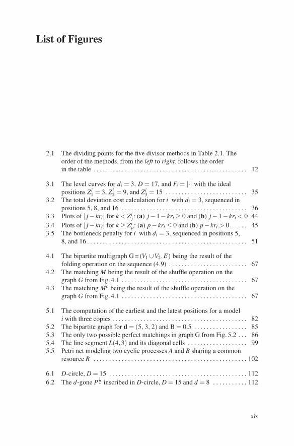
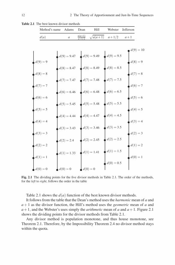
2.1 The dividing points for the five divisor methods in Table 2.1. Theorder of the methods, from the left to right, follows the orderin the table . . . . . . . . . . . . . . . . . . . . . . . . . . . . . . . . . . . . . . . . . . . . . . . . . 12

3.1 The level curves for di = 3, D = 17, and Fi = |·| with the idealpositions Zi

1 = 3, Zi2 = 9, and Zi

3 = 15 . . . . . . . . . . . . . . . . . . . . . . . . . . 353.2 The total deviation cost calculation for i with di = 3, sequenced in

positions 5, 8, and 16 . . . . . . . . . . . . . . . . . . . . . . . . . . . . . . . . . . . . . . . . 363.3 Plots of | j− kri| for k < Zi

j: (a) j−1− kri ≥ 0 and (b) j−1− kri < 0 443.4 Plots of | j− kri| for k ≥ Zi

p: (a) p− kri ≤ 0 and (b) p− kri > 0 . . . . . 453.5 The bottleneck penalty for i with di = 3, sequenced in positions 5,

8, and 16 . . . . . . . . . . . . . . . . . . . . . . . . . . . . . . . . . . . . . . . . . . . . . . . . . . . 51

4.1 The bipartite multigraph G = (V1∪V2,E) being the result of thefolding operation on the sequence (4.9) . . . . . . . . . . . . . . . . . . . . . . . . . 67

4.2 The matching M being the result of the shuffle operation on thegraph G from Fig. 4.1 . . . . . . . . . . . . . . . . . . . . . . . . . . . . . . . . . . . . . . . . 67

4.3 The matching Mc being the result of the shuffle operation on thegraph G from Fig. 4.1 . . . . . . . . . . . . . . . . . . . . . . . . . . . . . . . . . . . . . . . . 67

5.1 The computation of the earliest and the latest positions for a modeli with three copies . . . . . . . . . . . . . . . . . . . . . . . . . . . . . . . . . . . . . . . . . . . 82

5.2 The bipartite graph for d = (5, 3, 2) and B = 0.5 . . . . . . . . . . . . . . . . . 855.3 The only two possible perfect matchings in graph G from Fig. 5.2 . . . 865.4 The line segment L(4,3) and its diagonal cells . . . . . . . . . . . . . . . . . . . 995.5 Petri net modeling two cyclic processes A and B sharing a common

resource R . . . . . . . . . . . . . . . . . . . . . . . . . . . . . . . . . . . . . . . . . . . . . . . . . 102

6.1 D-circle, D = 15 . . . . . . . . . . . . . . . . . . . . . . . . . . . . . . . . . . . . . . . . . . . . 1126.2 The d-gone P

12 inscribed in D-circle, D = 15 and d = 8 . . . . . . . . . . . 112

xix

xx List of Figures

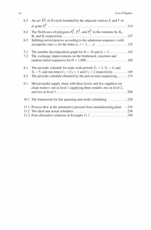
6.3 An arc XY of D-circle bounded by the adjacent vertices X and Y of

di-gone P12

i . . . . . . . . . . . . . . . . . . . . . . . . . . . . . . . . . . . . . . . . . . . . . . . . . 114

6.4 The North arcs of polygons P12

n , P12

i , and P12j in the rotations by θn,

θi, and θ j respectively . . . . . . . . . . . . . . . . . . . . . . . . . . . . . . . . . . . . . . . . 1276.5 Splitting arrival process according to the admission sequence s with

asymptotic rates ri for the letter ai, i = 1, . . .,n . . . . . . . . . . . . . . . . . . . 135

7.1 The number decomposition graph for D = 16 and di = 3 . . . . . . . . . . . 1457.2 The exchange improvements on the bottleneck, insertion and

random initial sequences for D = 1,000 . . . . . . . . . . . . . . . . . . . . . . . . . 160

8.1 The periodic schedule for tasks with periods T1 = 3, T2 = 4, andT5 = 5, and run-times C1 = C2 = 1 and C3 = 2 respectively . . . . . . . . . 169

8.2 The periodic schedule obtained by the just-in-time sequencing . . . . . . 174

9.1 Mixed-model supply chain with three levels and five suppliers (orchain nodes): one at level 1 supplying three models, two at level 2,and two at level 3 . . . . . . . . . . . . . . . . . . . . . . . . . . . . . . . . . . . . . . . . . . . . 208

10.1 The framework for fair queueing and stride scheduling . . . . . . . . . . . . 228

11.1 Process flow at the automotive pressure hose manufacturing plant . . . 25411.2 The ideal and actual schedules . . . . . . . . . . . . . . . . . . . . . . . . . . . . . . . . . 25811.3 Four alternative solutions in Example 11.1 . . . . . . . . . . . . . . . . . . . . . . 258

List of Tables

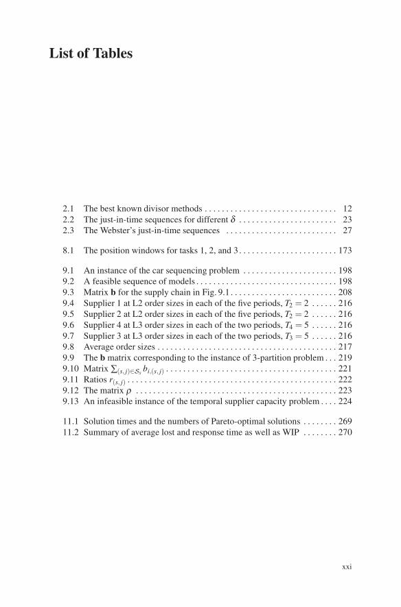
2.1 The best known divisor methods . . . . . . . . . . . . . . . . . . . . . . . . . . . . . . . 122.2 The just-in-time sequences for different δ . . . . . . . . . . . . . . . . . . . . . . . 232.3 The Webster’s just-in-time sequences . . . . . . . . . . . . . . . . . . . . . . . . . . 27

8.1 The position windows for tasks 1, 2, and 3 . . . . . . . . . . . . . . . . . . . . . . . 173

9.1 An instance of the car sequencing problem . . . . . . . . . . . . . . . . . . . . . . 1989.2 A feasible sequence of models . . . . . . . . . . . . . . . . . . . . . . . . . . . . . . . . . 1989.3 Matrix b for the supply chain in Fig. 9.1 . . . . . . . . . . . . . . . . . . . . . . . . . 2089.4 Supplier 1 at L2 order sizes in each of the five periods, T2 = 2 . . . . . . 2169.5 Supplier 2 at L2 order sizes in each of the five periods, T2 = 2 . . . . . . 2169.6 Supplier 4 at L3 order sizes in each of the two periods, T4 = 5 . . . . . . 2169.7 Supplier 3 at L3 order sizes in each of the two periods, T3 = 5 . . . . . . 2169.8 Average order sizes . . . . . . . . . . . . . . . . . . . . . . . . . . . . . . . . . . . . . . . . . . 2179.9 The b matrix corresponding to the instance of 3-partition problem . . . 2199.10 Matrix ∑(s, j)∈Ss bi,(s, j) . . . . . . . . . . . . . . . . . . . . . . . . . . . . . . . . . . . . . . . . 2219.11 Ratios r(s, j) . . . . . . . . . . . . . . . . . . . . . . . . . . . . . . . . . . . . . . . . . . . . . . . . . 2229.12 The matrix ρ . . . . . . . . . . . . . . . . . . . . . . . . . . . . . . . . . . . . . . . . . . . . . . . 2239.13 An infeasible instance of the temporal supplier capacity problem . . . . 224

11.1 Solution times and the numbers of Pareto-optimal solutions . . . . . . . . 26911.2 Summary of average lost and response time as well as WIP . . . . . . . . 270

xxi

Chapter 1Preliminaries

This chapter briefly reviews the basic terminology and notation used in the book.We begin with some notation and terminology borrowed from the formal languagetheory, see for instance Hopcroft and Ullman [9].

An alphabet A = {a1, . . .,an} is a finite non-empty set of symbols. A word (orsequence) S (we also use small s to denote sequence) over A is any finite sequenceof symbols from A. The length of S, that is the number of symbol occurrences inS, is denoted by |S|. The empty word, denoted by Λ, is the unique word over A oflength 0. The word

S = s1s2· · ·sm

where si ∈ A for i = 1, . . .,m will also be denoted as

S = s1→ s2→ ··· → sm.

The index i will be called the position of the letter si in the word S. If word S = S1S2

is the concatenation of words S1 and S2, then S1 is called a prefix of S, and S2 iscalled a suffix of S. For k = 1, . . ., |S|, the prefix made up of the first k symbols ofa non-empty word S is referred to as the k-prefix. For a word S and a non-negativeinteger m, the concatenation m times of S will be denoted as follows

SS. . .S︸ ︷︷ ︸

m−times

= (S)m = Sm.

The infinite repetition of word S will be denoted by

S∞,

and then S is called a cycle of S∞. For

S = s1s2· · ·sm

its mirror reflection SR isSR = sm· · ·s2s1.

W. Kubiak, Proportional Optimization and Fairness, International Series in Operations 1Research & Management Science 127, DOI 10.1007/978-0-387-87719-8 1,c© Springer Science+Business Media LLC 2009

2 1 Preliminaries

A sequence S is a palindrome if there is a sequence W such that

S = WW R.

We denote by A∗ the set of all finite words over A. The number of occurrencesof a given symbol a ∈ A in a word S ∈ A∗ is denoted by |S|a. Any occurrence of agiven symbol a in sequence S will also be referred to as a copy of the symbol.

The Parikh vector associated with a word S ∈ A∗ with respect to the alphabetA= {a1, . . .,an} is

(|S|a1 , . . ., |S|an).

A factor (subsequence) of length (size) b≥ 0 of S = s1s2· · ·sm is a word x such thatx = si . . . si+b−1.

We denote by R, Z, and N sets of real, integer, and natural numbers, respectively.Let {a1, . . .,an}Z be the set of infinite sequences on the alphabet A = {a1, . . .,an}.For the letter ai and an infinite sequence S ∈ {a1, . . .,an}Z let I(S,ai) ∈ {0,1}Z bethe indicator in S of the letter ai, that is I(S,ai) j = 1 if and only if s j = ai.

Let d1, . . .,dn be n≥ 1 positive integers called demands (or model demands) andlet the alphabet A = {1, . . .,n}. This particular alphabet will be most often used inthe book. Any letter i ∈ A will also be referred to as a model i, or a client i, or astate i, or a queue i depending on the context of our discussion. The vector

d = (d1, . . .,dn)

will be referred to as the vector of demands. We use the bold notation d,p,a, etc.for vectors in the book. We define the total demand

D = d1 + · · ·+ dn,

and the rates

ri =di

D

for letters i = 1, . . .,n. The vector of demands is called a standard instance if 0 <d1 ≤ d2 ≤ ·· · ≤ dn, n≥ 2, and the greatest common divisor of d1,d2, . . . ,dn,D is 1,that is gcd(d1, . . . ,dn,D) = 1.

Consider the set JIT of words on A all having their Parikh vectors with respectto A equal

d = (d1, . . .,dn).

Any, S ∈ JIT will be referred to as a just-in-time sequence or a just-in-time wordfor demand vector d, or simply just-in-time sequence. For S ∈ JIT, let xi,k be thenumber of letter i ∈A occurrences in the k− prefix, k = 1, . . .,D of w. We also writexik instead of xi,k.

The floor function �x of x is the greatest integer less than or equal to x. Theceiling function x� is the least integer greater that or equal to x, see Graham et al.[10] for more on these functions. The nearest integer function [x] or [x] 1

2is the

integer closest to x when the fractional part of x is equal to 12 we round downward

1 Preliminaries 3

unless otherwise specified. The |x| denotes the absolute value of any real x. Though,we use the same notation |.| for both the absolute value and the sequence length thecontext will clearly indicate which of the two applies.

The least common multiple of integers n1, . . .,nm, m ≥ 1, will be denoted bylcm(n1, . . .,nm). The greatest common divisor of non-zero integers n1, . . .,nm, m≥ 1,will be denoted by gcd(n1, . . .,nm). The notation di � D for positive integers di andD means that di does not divide D.

The infimum or greatest lower bound of a subset R of real numbers is denotedby inf(R) and is defined to be the biggest real number that is smaller than or equalto every number in R. If no such number exists (because R is not bounded below),then we define inf(S) = −∞.

Further terminology and notation will be introduced through the book.

Chapter 2The Theory of Apportionmentand Just-In-Time Sequences

2.1 Introduction

The apportionment problem and theory have their roots in the proportional represen-tation system intended for the House of Representatives of the United States whereeach state receives seats in the House proportionally to its population. This chapterreviews these results of the apportionment theory that are most relevant to the topicof just-in-time optimization. It follows the excellent expositions of the basics of thetheory presented in the books by Balinski and Young [2], and Young [3]. However,the chapter also includes new results obtained since these publications – especiallyin the context of the theory’s new applications presented in this book.

The apportionment theory has been developed to address the problem of fairrepresentation or “meeting the ideal of one man, one vote” as Balinski and Youngput it in the title of their book. This ideal is clearly a fundamental one yet, as onefeels, unattainable, and thus the apportionment problem is not just a problem inmathematics.

This book looks at this ideal in a broader than just political context in order torecognize the ideal’s universality. For instance, the clients or virtual clients payingfor the executions of their jobs in today’s distributed computational economies, seefor instance Waldspurger et al. [11], expect a fair implementation of these virtualeconomies – the clients demand a fair representation in terms of resource alloca-tions to their jobs so that the ideal of one currency unit spent equals any other spentin the same distributed economy is met. Thus, a client who pays twice as muchfor its job execution as another one would like to see its job progressing at twicethe rate of the other client’s similar job at any time. Another example is a protec-tion mechanism against antisocial behavior of individual hosts on the Internet and inother networks, see Nagle [12]. There, the apportionment methods can be used to es-tablish an accepted norm for a good behavior and can lead to the whole network in-creased stability. There are volume differences too, the apportionment methods usedtraditionally in proportional election or representation system are usually called towork every 4–5 years, whereas the same methods would be called millions of times

W. Kubiak, Proportional Optimization and Fairness, International Series in Operations 5Research & Management Science 127, DOI 10.1007/978-0-387-87719-8 2,c© Springer Science+Business Media LLC 2009

6 2 The Theory of Apportionment and Just-In-Time Sequences

every minute on the Internet proving their application huge volume. This volumerequires such apportionment methods that are computationally extremely efficientand relay on just few data in making online decisions as to who will receive theresources next. Fortunately, most apportionment methods, the divisor methods andin particular parametric methods for instance, satisfy all these conditions. Thus, theapportionment theory is where we feel any discussion of proportional representationshould start.

Section 2.2 defines the apportionment problem. Section 2.3 introduces the basicaxioms of the apportionment theory. These include the basic exact, anonymous andhomogenous apportionments as well as population monotone apportionments intro-duced to avoid undesirable anomalies. Section 2.4 presents the divisor methods ofapportionment. These are the only apportionment methods that deliver populationmonotone apportionments. Section 2.5 discusses incompatibility of being popula-tion monotone and staying within a quota properties of apportionment. Section 2.6focuses on these features of divisor methods that encourage coalitions and schisms.Section 2.7 shows how to construct the just-in-time sequences using the housemonotone apportionment methods. Section 2.8 discusses the desirable properties ofjust-in-time sequences inherited from the parametric apportionment methods. Theproperties include periodicity and various symmetries. Finally, Sect. 2.9 discussesthe consistency with a standard two-state solution which is unique for the Webster’smethod of apportionment.

2.2 The Apportionment Problem

The instance of the apportionment problem is defined by the integer house size h≥ 0and a positive real vector of state populations:

p = (p1, p2, p3, . . . , ps) > 0. (2.1)

An apportionment of h seats among s states is an integer vector

a = (a1,a2,a3, . . .,as)≥ 0 (2.2)

such that ∑si=1 ai = h.

Let the total population be

P =s

∑k=1

pk.

A “fair” share of state i seats is its quota

qi =pihP

.

2.3 Which Apportionment? 7

However, the quota vector

q = (q1,q2,q3, . . .,qs)

may be fractional and thus not an apportionment. We sometimes use the notationah and qh instead of a and q, respectively to emphasize that the latter two vectorscorrespond to the house of size h. We refer to

�qi=⌊

pihP

⌋

(2.3)

as the lower quota of state i and to

qi�=⌈

pihP

⌉

(2.4)

as the upper quota of the state.The solution to the apportionment problem is found by an apportionment

method M. The method maps the vector p and the house size h into a set M(p,h) ofapportionments a that satisfy the condition (2.2).

2.3 Which Apportionment?

The definition of the apportionment problem given in (2.2) may result into trivialthough unacceptable, for instance socially, solutions which need to be ruled outfrom further consideration. This is done by imposing axioms that define what issocially acceptable as properties of an apportionment. However, we believe thatthese properties should hold for other applications of the apportionment theory aswell. We begin with the basic properties.

2.3.1 The Basics: Exact, Anonymous and HomogeneousApportionments

We call the method M exact if

(q1, . . .,qs) ∈M(p,h) whenever quota qi =pihP

is an integer for all i,

and this solution is unique. A method is anonymous if for any permutation π of thestates 1, . . .,s we have

(a1,a2,a3, . . .,as) ∈M((p1, p2, p3, . . . , ps),h)

8 2 The Theory of Apportionment and Just-In-Time Sequences

if and only if

(aπ(1),aπ(2),aπ(3), . . .,aπ(s)) ∈M((pπ(1), pπ(2), pπ(3), . . . , pπ(s)),h)

for all population vectors p and house sizes h. That is permuting the state popula-tions results in apportionments that are permuted the same way.

An apportionment method M is homogeneous if for any p and h one requiresM(p,h) = M(λ p,h) for any positive rational number λ .

We continue the list of axioms with the not-so-obvious ones. These came to theattention of politicians and researchers as a result of infamous paradoxes or anom-alies that lead to abandoning some earlier used apportionment methods. The newaxioms were then formulated to protect against these paradoxes. We begin with themost famous one, the Alabama paradox, and its remedy, namely the house monotonemethods.

2.3.2 House Monotone Apportionments

Any apportionment method M(p,h) that gives an apportionment vector a for thehouse size h and the population vector p, and an apportionment vector a′ ≥ a forthe house of size h′ = h + 1 and the same population vector p is said to be housemonotone. Precisely, a method M is house monotone if for every p and h if a ∈M(p,h), then there is a′ ∈M(p,h + 1) such that a′ ≥ a. This books relies on ap-portionment methods for iteratively building sequences which requires the housesize h to grow. Thus, only house monotone methods are relevant for our discus-sion since they allow to extend a sequence without any change to it, that is towhat has already been built. All divisor methods defined later in Sect. 2.4.1 arehouse monotone. There are, however, historically important apportionment meth-ods that are not house monotone. The Alexander Hamilton’s method, known also asthe largest reminder method is an example of an apportionment method that is nothouse monotone. The Hamilton’s method lead to the infamous paradox of Alabamain 1882, when a larger size of the House gave fewer seats to the state of Alabama.The method’s failure to be house monotone can be illustrated by the following ex-ample with the population vector p = (6,6,1). The house size h = 5 results in quotas6×513 = 2 4

13 for the first two states and quota 513 for the third state, thus according to

the Hamilton’s method the apportionment is (2,2,1) since each state gets its wholenumber of seats, that is 2,2 and 0 respectively, first, and then since the total numberof seats apportioned is one less than the house size, the difference goes to the statewith the largest reminder, that is to the third state. Now, let us increase the size of thehouse to h = 6. Then, the quotas are 6×6

13 = 3613 = 2 10

13 for the first two states and 613 for

the third. Then, the Hamilton’s method results in the apportionment (3,3,0). Thus,the third state losses its only seat in a larger house – an example of the Alabamaparadox.

An even stronger axiom is the following population monotone axiom.

2.3 Which Apportionment? 9

2.3.3 Population Monotone Apportionments

The Alabama paradox reveals anomalies that some apportionment methods exhibitwhenever the size of the house h grows. However, it is not the only anomaly en-countered in the theory of apportionment. Other anomalies may show in case ofrapid changes in populations. One such anomaly is the population paradox, whichhappens whenever an apportionment method is not able to ensure that if the state ispopulation increases and the state js decreases, then state i gets no fewer seats andstate j gets no more seats with the new populations than they do with the originalones and the unchanged house size h. To avoid this population paradox as well asother paradoxes the population monotone apportionment methods have been intro-duced. Formally, the method is population monotone if for any two vectors of pop-ulations p,p′ > 0, house sizes h and h′, and vectors of apportionments a ∈M(p,h),a′ ∈M(p′,h′) the following implication holds

p′�p′k≥ pi

p j⇒

⎧

⎪

⎨

⎪

⎩

¬(a′� < ai∧a′k > a j)or

p′�p′k

= pip j

and a′�,a′k can be substituted for ai,a j in a

⎫

⎪

⎬

⎪

⎭

. (2.5)

The population monotone apportionment methods also avoid the new states paradoxthat may arise whenever the sates join the union. The new states paradox consists inthe following. Suppose a state s+1 joins in the union of s states. Then, this paradoxhappens whenever there are two states i and j of the old union such that one ofthem losses seats and the other gains seats. The population monotone apportionmentmethods avoid also the seceding states paradox. Suppose a state k secedes from theunion of s states. Then, the paradox happens if there are two states i and j otherthan k such that one of them losses seats and the other gains seats.

The next class of methods ensures that an apportionment that is satisfactory forall states remains so for any subset of states considered alone. For instance twocompeting jobs may monitor their own progress and compare it with each other ir-respectively of other jobs being present in the system and competing for the sameresources, see the peer-to-peer fairness in Chap. 10. The uniform apportionmentmethod ensures their satisfaction irrespective of other jobs.

2.3.4 Uniform Apportionments

An apportionment method is said to be uniform if it ensures that an apportion-ment a = (a1,a2, . . .,as) of h seats of the house among states with populationsp = (p1, p2, . . ., ps) will stay the same whenever it is restricted to any subset Sof these states and the house size ∑i∈S ai = h′. In other words, if for every t, 2 ≤t ≤ s, (a1, . . .,as) ∈M((p1, . . ., ps),h) implies (a1, . . .,at) ∈M((p1, . . ., pt),∑t

i=1 ai)and if also (b1, . . .,bt) ∈ M((p1, . . ., pt),∑t

i=1 ai), then (b1, . . .,bt ,at+1, . . .,as) ∈

10 2 The Theory of Apportionment and Just-In-Time Sequences

M((p1, . . ., ps),h). Each uniform method can be obtained by using a rank-indexfunction. The rank-index functions will be defined in Sect. 2.4.3.

Finally, the quota satisfaction property. This property however is at odds withpopulation monotonicity, see the Impossibility Theorem 2.4.

2.3.5 Apportionments Satisfying Quota

The apportionment of ai seats to state i satisfies the lower quota for populationvector p and house size h if and only if

�qi ≤ ai, (2.6)

and it satisfies the upper quota if and only if

ai ≤ qi� . (2.7)

The ai satisfies the quota if it simultaneously satisfies the lower and the upper quota,that is

�qi ≤ ai ≤ qi� . (2.8)

The apportionment vector a satisfies the quota if and only if it satisfies simultane-ously the lower and the upper quota for all states. The method M(p,h) satisfies thequota if each apportionment vector a ∈M(p,h) satisfies the quota for any p and h.

Though it may appear natural to request that an apportionment method stayswithin the quota this request has been virtually rejected by the apportionment the-ory since it can not be simultaneously met with the requirement of populationmonotonicity. The latter is considered more important for the apportionment. How-ever, staying within the quota gains importance in just-in-time applications whereit may be argued as being more important than population monotonicity due to itsability to closely track a target value.

We now turn to the apportionment methods themselves.

2.4 Apportionment Methods

2.4.1 Divisor Methods

One can argue that the most successful approach to apportionment is based on adeceptively simple and unquestionably natural idea that calls for calculating theideal district size x, or a divisor, that is the number of voters a single seat in thehouse ideally represents, and then checking how many such ideal districts fit intoeach state population. This latter number called quotient is then rounded to give the

2.4 Apportionment Methods 11

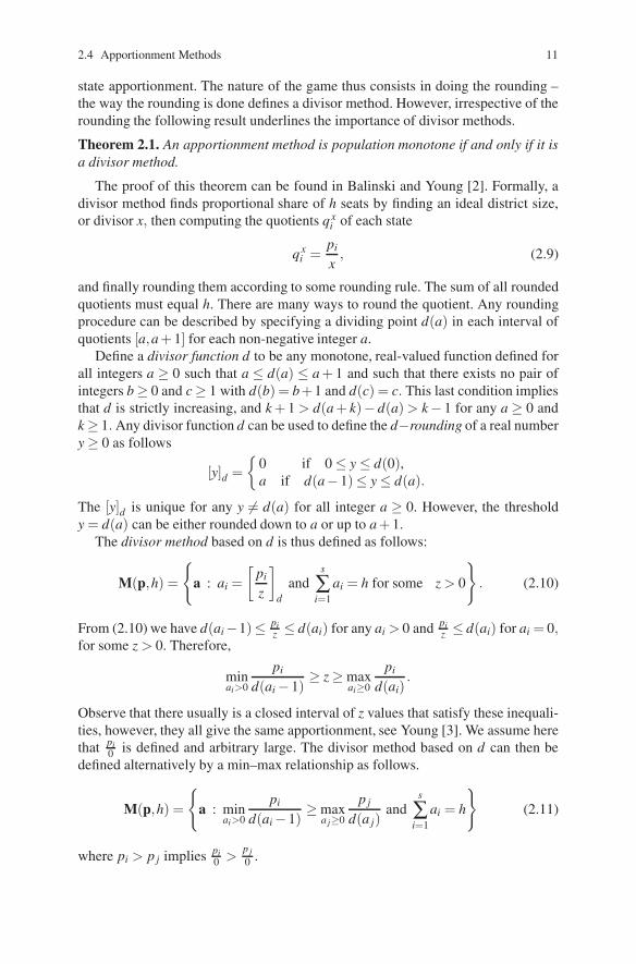
state apportionment. The nature of the game thus consists in doing the rounding –the way the rounding is done defines a divisor method. However, irrespective of therounding the following result underlines the importance of divisor methods.

Theorem 2.1. An apportionment method is population monotone if and only if it isa divisor method.

The proof of this theorem can be found in Balinski and Young [2]. Formally, adivisor method finds proportional share of h seats by finding an ideal district size,or divisor x, then computing the quotients qx

i of each state

qxi =

pi

x, (2.9)

and finally rounding them according to some rounding rule. The sum of all roundedquotients must equal h. There are many ways to round the quotient. Any roundingprocedure can be described by specifying a dividing point d(a) in each interval ofquotients [a,a + 1] for each non-negative integer a.

Define a divisor function d to be any monotone, real-valued function defined forall integers a ≥ 0 such that a ≤ d(a) ≤ a + 1 and such that there exists no pair ofintegers b≥ 0 and c≥ 1 with d(b) = b+1 and d(c) = c. This last condition impliesthat d is strictly increasing, and k + 1 > d(a + k)− d(a) > k− 1 for any a ≥ 0 andk≥ 1. Any divisor function d can be used to define the d−rounding of a real numbery≥ 0 as follows

[y]d ={

0 if 0≤ y≤ d(0),a if d(a−1)≤ y≤ d(a).

The [y]d is unique for any y �= d(a) for all integer a ≥ 0. However, the thresholdy = d(a) can be either rounded down to a or up to a + 1.

The divisor method based on d is thus defined as follows:

M(p,h) =

{

a : ai =[

pi

z

]

dand

s

∑i=1

ai = h for some z > 0

}

. (2.10)

From (2.10) we have d(ai−1)≤ piz ≤ d(ai) for any ai > 0 and pi

z ≤ d(ai) for ai = 0,for some z > 0. Therefore,

minai>0

pi

d(ai−1)≥ z≥max

ai≥0

pi

d(ai).

Observe that there usually is a closed interval of z values that satisfy these inequali-ties, however, they all give the same apportionment, see Young [3]. We assume herethat pi

0 is defined and arbitrary large. The divisor method based on d can then bedefined alternatively by a min–max relationship as follows.

M(p,h) =

{

a : minai>0

pi

d(ai−1)≥max

a j≥0

p j

d(a j)and

s

∑i=1

ai = h

}

(2.11)

where pi > p j implies pi0 >

p j0 .

12 2 The Theory of Apportionment and Just-In-Time Sequences

Table 2.1 The best known divisor methods

Method’s name Adams Dean Hill Webster Jefferson

d(a) a a(a+1)a+1/2

√

a(a+1) a+1/2 a+1

�d(0) = 0

�d(1) = 1

�d(2) = 2

�d(3) = 3

�d(4) = 4

�d(5) = 5

�d(6) = 6

�d(7) = 7

�d(8) = 8

�d(9) = 9

�d(0) = 0

�d(1) = 1.33

�d(2) = 2.4

�d(3) = 3.43

�d(4) = 4.44

�d(5) = 5.45

�d(6) = 6.46

�d(7) = 7.47

�d(8) = 8.47

�d(9) = 9.47

�d(0) = 0

�d(1) = 1.41

�d(2) = 2.45

�d(3) = 3.46

�d(4) = 4.47

�d(5) = 5.48

�d(6) = 6.48

�d(7) = 7.48

�d(8) = 8.49

�d(9) = 9.49

�d(0) = 0.5

�d(1) = 1.5

�d(2) = 2.5

�d(3) = 3.5

�d(4) = 4.5

�d(5) = 5.5

�d(6) = 6.5

�d(7) = 7.5

�d(8) = 8.5

�d(9) = 9.5

�d(0) = 1

�d(1) = 2

�d(2) = 3

�d(3) = 4

�d(4) = 5

�d(5) = 6

�d(6) = 7

�d(7) = 8

�d(8) = 9

�d(9) = 10

Fig. 2.1 The dividing points for the five divisor methods in Table 2.1. The order of the methods,for the left to right, follows the order in the table

Table 2.1 shows the d(a) function of the best known divisor methods.It follows from the table that the Dean’s method uses the harmonic mean of a and

a + 1 as the divisor function, the Hill’s method uses the geometric mean of a anda+1, and the Webster’s uses simply the arithmetic mean of a and a+1. Figure 2.1shows the dividing points for the divisor methods from Table 2.1.

Any divisor method is population monotone, and thus house monotone, seeTheorem 2.1. Therefore, by the Impossibility Theorem 2.4 no divisor method stayswithin the quota.

2.4 Apportionment Methods 13

2.4.2 Parametric Methods

Parametric method φδ is a divisor method with d(a) = a+δ , where 0≤ δ ≤ 1. Theparametric methods are of interest for two reasons. First, they are clearly computa-tionally very efficient, their divisor functions are linear. Second, they generate cyclicjust-in-time sequences whereas the divisor methods which are not parametric do notalways generate cyclic just-in-time sequences. This will be shown in Theorem 2.12.

Clearly, the Adams’s, Webster’s (known also as the Sainte-Lague’s method) andJefferson’s (known also as the d’Hondt’s method) methods are parametric, while theDean’s and Hill’s are not.

2.4.3 Rank-Index Methods

The idea behind the rank-index methods is to define a standard of comparison or therank-index function, see Young [3], and then use it to obtain an equitable allocationrelative to that standard. An allocation is equitable relative to a rank-index functionif no seat transfer is justified. The seat transfer is justified if there are i and j so that jcan give up one seat to i and by doing so reduce the inequity between the two states,that is if the following inequality is satisfied

∣

∣r(pi,ai)− r(p j,a j)∣

∣ >∣

∣r(pi,ai + 1)− r(p j,a j−1)∣

∣ .

The rank-index function is any real-valued function of rational p and integer a ≥ 0that is decreasing in a, that is r(p,a− 1) > r(p,a) for any p and a ≥ 1. The rank-index methods begin apportionment of h seats with defining a rank-index functionr(p,a) on all possible pairs (p,a) where p is a state population and a is any integerbetween 0 and h. The pairs (p,a) are then ordered in descending order of their rank-index values. The h seats are then apportioned according with the first h pairs on theordered list. Thus, the h seats are apportioned to the most deserving, according to therank-index, states.

An equitable allocation can also be found by the following simple algorithmgiven in Balinski and Young [2]. Let F be the family of functions f defined asfollows.

1. For h = 0 let f (p,0) = 0.2. If f (p,h) = a, then f (p,h+1) is found by giving ai +1 seats to some state i such

that r(pi,ai)≥ r(p j,a j) for all j, and a j seats to each j �= i.

The rank-index method based on r(p,a) is defined as follows:

M(p,h) = {a : a = f (p,h) f or some f ∈ F}. (2.12)

Any function of the form r(p,a) = pd(a) with a divisor function d(a) is a rank-index

function since pd(a−1) > p

d(a) by definition of divisor functions. Therefore, we canequivalently define the divisor method as follows, see Balinski and Young [2].