Embed Size (px)
Citation preview

© The Authors.
All rights reserved. No part of this publication may be reproduced without the permission of the authors.
http://graduateinstitute.ch/ctei
CTEI Working Papers
International Production Sharing: Insights from Exploratory Network Analysisa
Yose Rizal Damuri
Abstract
The phenomenon of international production sharing, in which production is broken up into smaller bits of tasks and locate them in separate places, has been observed globally in the last several decades. While it has been getting a lot of attention, it is still not clear how to define and examine the trend. In this paper, some statistical methods borrowed from network analysis and graph theory provide aalternative way to see the pattern and structure of global production network. The availability of new input-output data complements the analysis by providing information on international production link beyond what trade data could reveal.
a This paper is part of research under the ProDoc Trade Programme. It was presented at Geneva Trade and Development Workshop on 5th April 2011 at the World Trade Organization.b Graduate Institute of International and Development Studies for Trade and Economic Integration
CTEI PAPER
CTEI
All rights reserved. No part of this publication may be reproduced without the permission of the authors.
CTEI Working Papers
International Production Sharing: Insights from Exploratory Network
Yose Rizal Damurib
The phenomenon of international production sharing, in which production is broken up into smaller bits of tasks and locate them in separate places, has been widely observed globally in the last several decades. While it has been getting a lot of attention, it is still not clear how to define and examine the trend. In this paper, some statistical methods borrowed from network analysis and graph theory provide aalternative way to see the pattern and structure of global production network. The
output data complements the analysis by providing information on international production link beyond what trade data could reveal.
This paper is part of research under the ProDoc Trade Programme. It was presented at Geneva Trade
and Development Workshop on 5th April 2011 at the World Trade Organization.. Graduate Institute of International and Development Studies for Trade and Economic Integration
CTEI PAPERS
CTEI-2012-3
All rights reserved. No part of this publication may be reproduced without the permission of the authors.
International Production Sharing: Insights from Exploratory Network
The phenomenon of international production sharing, in which production is broken widely
observed globally in the last several decades. While it has been getting a lot of attention, it is still not clear how to define and examine the trend. In this paper, some statistical methods borrowed from network analysis and graph theory provide an alternative way to see the pattern and structure of global production network. The
information on international production link beyond what trade data could reveal.
This paper is part of research under the ProDoc Trade Programme. It was presented at Geneva Trade
Graduate Institute of International and Development Studies for Trade and Economic Integration

CTEI PAPERS
CTEI-2012-3
http://graduateinstitute.ch/ctei
ProDoc Trade Programme
The ProDoc Trade is a research and training programme that brings together PhD students and professors from the University of Geneva, the University of Lausanne and the Graduate Institute of International and Development studies, as well as economists working in the Geneva-based International Organisations devoted to trade (mainly the WTO, ITC and UNCTAD). This networking aims at an agglomeration of excellence in research and making the Lémanique area the heart of international trade economics attractive to trade scholars world wide and to first-rate students from around the globe.
www.graduateinstitute.ch/ctei
Centre for Trade and Economic Integration (CTEI)
The Centre for Trade and Economic Integration fosters world-class multidisciplinary scholarship aimed at developing solutions to problems facing the international trade system and economic integration more generally. It works in association with public sector and private sector actors, giving special prominence to Geneva-based International Organisations such as the WTO and UNCTAD. The Centre also bridges gaps between the scholarly and policymaking communities through outreach and training activities in Geneva.
www.graduateinstitute.ch/ctei

International Production Sharing: Insights from Exploratory Network Analysis
1 Introduction
1.1 Background of Study For the last couple of decades, a new international business model has been sharpening the
development of global manufacturing industry. This emerging trend, know as production
sharing, defines production process at a finer level of tasks than the conventional model1.
The core of this evolving business model is to break up production process into smaller bits
of tasks and to place them in separate places, usually cross-border locations. These
segmented activities can then be reintegrated again through a system of international value
chains and international production networks.
The main goal of placing smaller fragments of production process on different location is to
take advantage of economic differences among different locations and countries. Different
stages of production may be located at places where costs of production are the lowest. That
would be done by matching different factor intensities for each production stage to factor
abundance of locations. By allowing production process to flow across border, firms could
exploit differences in international factor endowments more comprehensively.
As a growing business and production model, this international fragmentation of production
has been discussed in many studies and analysis. The next sub-section of this introduction
discusses in more detail several theoretical and empirical attempts to examine the trend.
However, despite a lot of academic and scholarly attention, there is no clear method to
examine the prevalence of global production sharing. Even some very basic questions
remain unanswered: What is the magnitude of this practice? Which countries play more
important role? On what position?
This paper proposes new approach to examine international production sharing, particularly
with regard to measurement issues in order to address numerous basic questions on the
extents of this recent practice. Some statistical and mathematical methods borrowed from
network analysis and graph theory provide an alternative way to see the pattern and
1 This division of production into stages is known in many other designations, such as vertical specialization (Hummels et al. 2001), product fragmentation (Jones and Kierzkowski 2001), the 2nd production unbundling (Baldwin, 2006), or simply production network. In this paper, those terms are used interchangeably with the term production sharing.

structure of global production network. The availability of new data on input-output table
enables us to see product fragmentation as a network flow of production across countries.
The main contribution of this paper into the literature is to provide better methodology to
measure the extent of product fragmentation, as well as proposing new concept in
examining the phenomena by putting it into network perspective. This approach provides
clearer insights on structure and pattern of the developing production network. Better
understanding on its structure and pattern is important for further examination of
international production sharing network.
After this introduction and review on related literatures and existing method, the paper
examines the change in trade pattern with relation to the development of global production
network. In particular we are interested in exploring whether there are tendency towards
regionalization and globalization of production sharing. The next section explores proposed
alternative measurement of production network by manipulating information from newly
available input-output table, based on some stochastic principles and features. Markov-
process type of random walk is introduced in an attempt to track the path of international
production flow and value added in a particular sector, allowing us to get various
characteristics of this international production network. The paper is concluded by
summarizing discussion in the final section.
1.2 International Production Sharing: Literature and Methods The trend of international production unbundling has attracted scholarly attention from
various perspectives. Earliest appraisals come from business and management point of view,
with the emphasis on management of supply and value chain. While most of these
literatures come up as part of study in multinational companies, some also discuss more
general aspects of international production and management. For example, OLI framework
of international business presents location as one factor that firms need to chose in order to
optimize their operation (Dunning 1989).
Literatures on supply and value chain remain an important contributor to the discussion on
international production sharing by providing illustrations and case studies on the operation
of particular firms or industries. Linden et al. (2007), for example, presents the case of
globalized value chain in the well known Apple’s product iPod.
From trade perspective, fragmentation of production has introduced a new line of thinking
that somewhat different than traditional Ricardian trade model (Baldwin 2006).

International exchange of final goods as proposed by traditional model become less
important as technological advance and reduction of transport cost have opened “the black-
boxes” of production entity, which are previously organized within a single firm located in
one site or in close proximity.
Important references on the theoretical framework of production fragmentation comes from
Jones and Kierzkowski, which explore the underlying motivations and reasons for firms to
choose their production centers fragmented in several locations (1990, 2001), as well as the
impacts of such activities (1998), although some works on trade in intermediate inputs can
be found in earlier literatures (for example Batra and Casas 1973, or Dixit and Grossman
1982). These papers suggest that variation in factor intensity of production stages and
differences in relative endowments across countries, together with technical progress in
related service links, make cross-border production sharing feasible and profitable.
Other theoretical works focus on the implications of this practice on structure of production,
prices, and wages to both recipient and sending countries2. Production sharing is also
commonly attributed to liberalization of trade, in particular with regard to regional
integration. Since cross-border relocation of different stages of production can happen
through international trade in intermediate inputs, trade liberalization among countries in the
same region might enhance production sharing in the region3.
Empirical literatures on international production sharing focus on looking at patterns of the
network; how they evolve over time; and the impacts of such development onto other
aspects. Some studies present the importance of international production unbundling and
intermediate goods into productivity at micro (firm) level, such as Amity and Konings
(2007), which describes the positive impact of liberalization in intermediate goods in
Indonesia to the firm productivity. Others try to identify the characteristics of firms involve
in such network, such as competition in the industry where production sharing usually takes
place (Paul and Wooster, 2008).
At aggregate level, Egger and Egger (2001), using outward processing data of EU countries,
find that outward processing, as a measure of production unbundling activities, is more
2 See for example Venables (1999), Markusen (2005), Grossman and Rossi-Hansberg (2006) and Baldwin and Robert-Nicoud (2007). Most of these papers work on a general equilibrium setting in the style of H-O model where price equalization does not occur as a result of international trade. 3 The link between regional integration and production fragmentation is usually examined descriptively. Some exceptions include the works from Arndt (2002), which employ mathematical modelling to address the issue.

prevalent in import competing industries, and negatively affects skill intensity in net-
exporting industries. On the effect to economic growth, Baldone et al. (2007) estimates
international production sharing contribute more to economic activities than the traditional
trade activities in final products.
Another type of empirical literatures on international production sharing concerns more on
the measurement and pattern of this practice in relation to international trade. These works
attempts to give meaningful description on the prevalence of international product
fragmentation by considering various different aspects and complexity of the phenomena.
Since this type of study is more related to discussion in this paper, we take a look at the
literature in more detail by putting the associated works into categories based on their
methodologies.
Current Methods of Assessment There are three main methodologies and data sources that have been used in measuring the
prevalence of international production unbundling: customs statistics based on special
scheme of trade; international trade statistics in parts and components; and input output
table of production.
The first method relies on the availability of customs statistics that record trade activities
under special schemes of tariff reduction or exemption. Many countries, in order to give
incentives for domestic industrial development provide tariff exemption for imported inputs
that are used further for exporting goods (this is mostly the case of developing countries), or
for domestic input content of imported final products (the case of developed countries). The
special scheme usually makes the customs official to record the trade activities under a
special heading. This special heading allows trade scholars to obtain a narrow measure of
international production network. Swenson (2005), for example, examines the US offshore
assembly program (OAP), which record input contents of import originated fro the US, and
find that offshoring activities grew significantly during the period of 1980-2000. Egger and
Egger (2005) also present similar result for the outward processing trade (OPT) program of
EU, particularly with Central Eastern European countries.
The problem with this method is the availability of data. Besides EU’s OPT and US’s OAP
statistics, only a handful of countries make this statistics available. To our knowledge only
China among other major trade player which make this statistics available. Lemoine and
Ünal-Kesenci (2004) assess China’s assembly trade statistics and shows that China's

outstanding performance can be linked to its integration in the international production
network. Another difficulty with the method is related to the general trend of tariff
reduction. As tariff rate on parts and components becomes lower, firms’ incentives to use
such special schemes is decreasing, resulting to poorer coverage of the international use of
intermediate goods.
Certain categorization of trade statistics can also be used to indicate the occurrence of
international production unbundling. Standard International Trade Classification (SITC)
version 2 and 3 classify trade statistics into category loosely based on stage of production.
These classifications allow trade scholars to identify certain products related to the
incidence of production unbundling, especially with the case of manufacturing and
machinery production4. This type of work is initiated by Yeats (1998), which finds that trade
in parts of components of machinery accounts for more than 30% of total OECD countries
exports. Other works used this method extensively, particularly in looking at production
fragmentation with focus on several specific regions. The extensive use of the method is
understandable as the data can be easily collected and offer intensive coverage in terms of
regions, period, and also products5.
Despite its popularity due to easily accessible data and wide coverage of analysis, this
method suffers from several important problems. The most important one is double
recording in trade statistics, especially in machinery products. Car windshield produced in
country A exported to country B for assembly process, would be counted again as B’s
exports, although there is no production transformation on that product. High prevalence of
cross border shipping of the same product makes this problem worse. Another problem is
related to the use of imported inputs. When import of a particular intermediate input takes
place, it is not clear of the use of this product, whether it would be used directly by
consumer as a replacement for broken product, or used by a producer for further production
process.
To deal with that problem, Hummels et al. (2001) proposes the calculation of vertical
specialization index (VS), which is based on the import content of exports using information
from input output (IO) table. The study finds that VS activities of ten OECD members grew
4 With machinery, this paper refers to the classification of SITC heading 7 (version 2 and 3), which covers general machinery, electrical and electronics, and motor vehicle and other transportation. 5 Many studies on regional importance of production network, such as studies on the so called “Factory Asia”, use this particular method. See for example Kimura and Ando (2004),

almost 30% since 1970 and account for more than 20% of the exports. Other studies extend
the coverage of the method and offer modifications from the original formulation to look at
other specific aspects of international production sharing, such as the work from Chen et al.
(2005) which uses more recent data and cover more regions; or the work from Johnson and
Noguera (2009) which extends the use of information from IO to compute bilateral trade in
value added; or Inomata (2008) that tries to capture the entire structure of production chain
using international input output table.
The accuracy of this method depends largely on the breakdown of production sector in IO
table. More detail breakdown provides better information on how production process
identified and tracked in the economy. This is the important problem of using IO table, as
there is no international standard classification of production in the table, making it difficult
to use it for international comparison. Moreover, most countries only provide less detail
breakdown of production, which often not enough to see the importance of international
production network. Another problem is related to the frequency of publication of such data,
which is usually produced every five years, making it difficult to be combined with
international trade statistics.
The most important limitation of this method, however, comes from the fact that input-
output tables are constructed basically at national level, having no or little information on
the international aspects. In order to examine the prevalence of international product
fragmentations, the information from IO should be combined by trade data, along with
certain assumptions in mind. Nevertheless, this method offers clearer measurements and
understanding of the international production unbundling.
This paper adopts the second and third methods in looking at global production networks
using the information from trade data and IO table. The methods proposed in this paper
differ from the existing literature on the measurements of international production sharing in
at least two aspects: the analysis is based on methods developed in exploratory network
analysis that takes into account not only bilateral relations, but also capturing the whole
structure of the network; in addition, the framework proposed in this study allows inference
of various features and characteristics of the cross-border flow of production and value
added at the aggregate level.

2 Global Production Unbundling: What Trade Data Reveals? As mentioned in the previous section, the method of analyzing international production
sharing by looking at trade data has some notable drawbacks. However, it also offers widest
coverage in looking at the network of production. This section explores the global patterns
of international production unbundling by looking at trade in parts and components of
machinery products. The purpose of this section is to examine the development of trade in
parts and components, as one of the most important aspect of production unbundling, and to
analyze certain patterns in the development of trade network.
Specifically, this section examines whether the growing production unbundling phenomena
tend to be regionally concentrated as many observers presented6. While stories of
international production network can be observed strongly in the East Asia region, the
globalization of production and trade in manufacturing products has also taken place in
other parts of the world. However, whether those countries are integrated regionally would
require more careful examination. In this section, we explore the structure of the
international production unbundling network that can be observed from data of international
trade in parts and components.
2.1 Global Network of Trade in Parts and Components A majority of studies in global trade and production unbundling is either to look at the basic
trend and structure of trade flows at the total level (see Fenstra 1998 and Yeats 2001), to
focus on regional structure of the trade (see Kimura and Ando 2005), or case studies of
several countries. Rarely analysis has been done on bilateral trade patterns in parts and
components, particularly involving global patterns of trade7. Analyzing bilateral trade
matrices reveals patterns of triangular and multilateral links between countries, which is
usually unseen in total trade flow. It becomes more important in the case of parts and
components as the products are often imported from one country to which they are later
passed downstream of the value chain in other countries.
One obstacle in doing that analysis is obvious: the structure is too big to be analyzed
descriptively. With over 100 countries with considerable value of trade, the matrix of global
trade consists of thousands of possible trade flows that make it difficult to handle with
6 See the literature review in the previous section 7 Some authors, such as Athukorala and Yamashita (2006) examines international production network being developed in East Asia in a global context. But only looks at the pattern of trade aggregated at regional or global level, instead of on bilateral basis.
conventional methods. Network Analysis (NA) provides some useful tools in analyzing
global bilateral trade flow. In the network analysis, structure of global bilateral trade can be
seen as a network of relation, in which countries are symbolized as the nodes or actors of the
network and the amount of bilateral trade represents strength of a directed (export or import)
relations between them.
The application of NA in analyzing global trade network can be traced back to the early
1990s with the publication of a paper from Smith and White (1992) which tries to identify
the roles of countries played in the global trading network and its evolution. Some later
papers concern more on the technical aspects of the global trade network, such as its
topological features and relational characteristics (see for example Kali and Reyes 2007).
While some methods of network analysis fit the needs in examining international trade
network, the application of NA’s techniques to trade statistics needs careful consideration.
Many methods in network analysis see pair-wise relations more than just relation between
two parties involved. In fact, network analysis is developed to examine relations beyond
direct bilateral connections. In friendship relation, for example, not only direct friends that
matter, but also friends of friends affect the network of friendship relation. Application of
network analysis to friendship connection, e.g. online social network, normally explores the
extents of these “higher orders” relations.
This nature of NA’s methods would be beneficial in looking at international production
sharing, in which production moves among many countries before being consumed, and not
only bilateral trade connection that matters. Unfortunately, bilateral trade statistic is built on
the assumption that trade involves only two countries; it is the flow of final goods from one
country to another, where it would be directly consumed in the destination country. The
extents of higher order relations in trade network can not be appropriately derived from this
bilateral direct relation, particularly not from the value of trade.
There are two ways to deal with this problem. One way is to choose methods of network
analysis dealing with this type of bilateral connection. Several methods in network analysis
and graph theory consider direct bilateral relation as similarity or distance between objects.
These methods are suitable for the application of network analysis on the structure and
pattern of bilateral trade relations in parts and components. We will apply relevant
techniques by assuming that bilateral trade relations are in line with proximity between
countries.

Alternatively is to reconstruct trade statistics to suit the nature of network analysis. This can
be done by looking at relations in production sharing as a network flow of production or
value added, streaming from one country to others until the production flows out of the
network, consumed as a final good. With this reconstructed data of international production
flow, many techniques of network analysis can be employed to examine properties of global
network of production sharing. This section mainly discusses the application of the first
procedure, while the latter part of this paper introduces to the alternative.
2.2 Structure of Trade Network Before going into more detail analysis of global trade network of parts and components, it is
worthwhile to say something about the data being used. A dataset of bilateral trade of parts
and components has been constructed using data from the UN Comtrade Database. The
classification of parts and components in this study follows the classification used in
Kimura (2007) as described in Appendix A8. In assessing changes over time, it is also
important to note that the dataset is not a balanced panel and the number of countries
changes over time. This occurs mainly due to the creation of new countries and the
abolishment of the old ones, as well as additional data from a large number of unreported
countries in the past.
In order to reduce the number of missing value from the dataset, but at the same time cover
a substantial number of countries, only countries with total exports of more than one billion
US dollar in 2005 are included in the sample. In the end the sample covers 100 countries for
the period of 1985 and 113 countries for 2005.
Table 1 presents some basic features of the dataset. From the table we can see that the
number of countries involve in parts and components trade increase over the period of
observation. Of all countries with reported data in mid 1980’s, only less than 60% recorded
some amount of exports of parts and components products, while the percentage increases to
87% in 2008. Trade in parts and components has also gain importance in the last three
decades, with an increase of more than 3 percentage point over its share in the world total
trade within 20 years of time. Note that the share of parts and components trade slightly falls
in the wake of 2008 crisis, while the number of exporters and countries being involved in
the trade activities has also declined.
8 There are other attempts to classify intermediate inputs (see Yeats 1998, for example). The classification used in this study is based on SITC version 2, comprising intermediate inputs used in machinery production.

Table 1. Trade in Parts and Components
Value / No. % Value / No. % Value / No. % Value / No. %
World Exports of Parts and Components1 163 9.99 594 12.24 1,320 13.00 1,760 11.56
Number of Country Pairs with the non zero trade2
- Manufacture 4,760 61.25 7,637 72.35 10,283 77.76 9,779 82.97
- Machinery 4,212 54.19 6,873 65.11 9,549 72.21 9,264 78.60
- Parts and Components 3224 41.48 5631 53.34 8254 62.42 8202 69.59
Exporters of Parts and Components3
58 58.59 88 84.62 113 99.12 102 87.181) Value in US$ billions; percentage of total world exports; 2) Percentage of non-missing country pairs3) Percentage of non-missing exporters
1985 1995 2005 2008
One characteristic of trade in parts and components presented in Table 1 is that only a
relatively small number of countries are involved in the network. While more than 60% of
possible country pairs exchange manufacture goods in the mid 1980’s, only around 40%
engage in parts and components trade. A more detail observation also reveals that the
biggest ten exporters of parts and components contribute to more than 88% of the world
market in 1985, and remain concentrated in 2005, although the figure declines to around
67%.
Table 2 provides more information on how trade in this type of product spreads out. The
USA and Japan dominate the market of parts and components in most of the period of
observation, while Germany overtakes the second place in 2005. Looking at the mean and
the standard deviation of each country in the table raises a suspicion that the destinations of
these countries’ exports are also rather concentrated. Relatively large values of standard
deviations compare to the means indicate that some destinations are more important to these
exporters than others. In order to give more insights on the structure of parts and
components trade network, we will turn to network analysis.
Table 2. Ten Biggests Exporters of Parts and Components

Country Exports Share (%) MeanStandard Deviation Country Exports Share (%) Mean
Standard Deviation
USA 49,200 30.18 424.5 1,306.3 USA 163,000 12.35 1,404.2 4,515.7
JPN 22,700 13.93 195.3 875.4 DEU 143,000 10.83 1,231.3 2,611.5
DEU 20,200 12.39 174.2 407.9 CHN 124,000 9.39 1,073.3 3,947.0
GBR 13,500 8.28 116.4 299.5 JPN 112,000 8.48 963.2 3,266.6
CAN 10,900 6.69 93.9 908.5 HKG 76,500 5.80 659.6 4,130.6
FRA 10,000 6.13 86.4 225.9 GBR 60,200 4.56 518.8 1,276.3
ITA 6,803 4.17 58.6 160.0 KOR 59,400 4.50 511.9 1,691.3
SWE 4,514 2.77 38.9 85.0 FRA 53,100 4.02 457.9 1,200.9
NLD 3,595 2.21 31.0 98.7 SGP 50,400 3.82 434.3 1,291.6
HKG 2,876 1.76 24.8 139.4 ITA 45,200 3.42 389.3 998.5
1985 2005
Some Basic Measures of Network To facilitate the analysis, trade data is constructed in a graph form. Let G = (V,E,w) be a
connected, weighted, and directed graph of trade relations, consisting of a set of nodes, or
vertices V, which represents the set of countries in our sample, and a set of edges E⊂ V×V .
Each edge represents E(r,s) trade relation between two countries r and s with trade values
assigned as non-negative real weight wrs. The graph can be written in a matrix W={wrs}
where rs-th element is represented by the corresponding weight wrs. In some cases it is also
useful to define the graph in its binary form by having it as v×v adjacency matrix A={ars}
where ars∈{0,1} by letting ars=1 if wrs>0, and zero otherwise.
The most simple but useful measure in examining the structure of a network is the vertex
degree, which is defined as the number of links that a given node has established; it simply
means how many partners that a particular country has trade relations with. Another concept
is vertex strength defined as the sum of weights associated to the links held by any given
vertex, or country. It is the sum of trade volume to all partners for each country. Vertex
degree (VD) and vertex strength (VS) of country r is then defined as follow.
vectorvaiswherewVS
aVD
VVs
rsr
Vs
rsr
1×==
==
∑
∑
ιιW
ιA
Both are important since the distribution of those indicators hint at certain topological
characteristics of the network structure. In a random network, i.e. a network consists of
nodes with randomly placed connections, the distribution of vertex linkages follows a bell-
shaped curve. In a scale-free network, where most nodes only have few connections and few

have many connections – the network normally takes form as hub and spoke -, the
distribution of VD and VS tends to follow power law (Barabási and Bonabeu 2003).
Figure 1.a Kernel density of VD Figure 1.b Kernel Density of VS
Figure 1.a and 1.b provide the kernel estimation of VD and VS trade network in parts and
components for 1985 and 2005. The noticeable feature of the degree distribution is
bimodality that appears both in 1985 and 2005. Most countries either trade with less than
50% of total countries, i.e. poorly connected to the network, or have extremely well trade
relations with almost all countries. However, the bimodality of the two distributions is
somewhat different. In 1985, low connected countries were more abundant than the well
connected ones. But the opposite situation can be observed in 2005.
From the distribution of vertex degree, it is difficult to conclude topological characteristic of
the network structure, as the distribution hardly follows certain parametrical distributions.
But for trade relations, looking at the volume of bilateral trade might be more insightful than
just to see whether there is a bilateral connection or not. That is why distribution of VS
might give better information than just the distribution of VD. Kernel density distributions
of countries’ trade value both for 1985 and 2005 follow the power law feature, at least
asymptotically.
This shape of distribution suggests some characteristics of scale-free network, in which hub
and spoke relations are found. From this simple analysis we can suspect that hub and spoke
trade connections, where few countries have many important connections and many
countries have few important connections, can be observed from trade relation in parts and
components. We will analyze this characteristic in more detail later in this section by
applying other technique from graph theory.

Another network characteristic worth mentioning with regards to our further analysis is the
network symmetry. One way to measure for the network symmetry is by applying an index
developed by Fagiolo (2006) based on the norm of the adjacency and weight matrix. The
index can be expressed in a formula below.
1
1
2
~2
2
−+′−
=n
nS
F
F
Q
QQ where IWQ )1( iiw−−= ;
∑∑=s r
rsFa22
Q is the Frobenius norm of the matrix Q
The index ranges from 0 (full symmetry) to 1 (full asymmetry). The application of the
formula to trade network matrix W reveals that the symmetry index is 0.28 and 0.31 for
1985 and 2005 respectively. These indicate certain level of symmetry for the network
although far from perfect symmetry. This result gives support to our treatment of trade data
in the next analysis: dealing with trade data as proximity data between countries. In other
words, we treat bilateral trade relations as symmetric assuming that countries pursue
bilateral balance trade regime. This enables us to apply appropriate network analysis
techniques as discussed previously.
Treating bilateral trade relations as symmetric may result to the loss of some useful
information. It is possible that trade between two countries is very much skewed towards
one partner, making the balance trade assumption affects validity of the results. However,
relatively low index of symmetry suggests that the loss may not be that severe, particularly
compare to the advantages from the application of appropriate network methods. Keeping
this in mind, the next analysis looks at trade relations as proximity between countries and
treats the network as an undirected one.
Maximum Spanning Tree One powerful method offered by network analysis is the visualization of a network by
drawing the relationships between nodes as lines or arcs. Despite that visualization can
provide numerous useful insights, a graph of a network becomes more difficult to interpret
when the number of nodes is large, particularly for a very dense network like global trade
network, where many countries are connected to almost all other nations. To overcome that
limitation, numerous methods have been developed to provide clearer interpretation of
network visualization. We look at the application of some of those methods to the network
of trade in parts and components.

As explained earlier, the analysis conducted in this section considers bilateral trade relation
as similarity or distance. Therefore it is important to make the matrix W symmetric, or to
create an un-directed graph G=(V,E,w) where wrs= wsr. It is equivalent to the assumption
that bilateral trade is balance. A geometric mean of bilateral trade relations is used in place
of the original trade data.
21
)( srrssrrs wwww ==
One simple but useful technique in network visualization to explore the structure of
relations between nodes is maximum spanning tree (MST) technique. Given a connected
graph G = (V,E,w), the MST is a sub-graph (V,T) such that T is a spanning tree with the
maximum total weight. A spanning tree T is a tree which links all vertices in the graph
together, while the trees in graph G refers to the sub-graph T in which any two vertices are
connected by exactly one edge.
A spanning tree of trade network is a connected graph which links a set of countries together
in such a way that there is only one connection between any pair. Therefore the maximum
spanning tree of trade network only presents the most important trade relation between two
countries, which maximizes the total trade relation in the network. By only focusing to the
most important bilateral connection, the structure of the network is more noticeable and easy
to see.
The technique used in this analysis is known as Kruskal’s algorithm (Kruskal 1956).
Kruskal’s algorithm works iteratively by selecting and adding an edge E(r,s) in decreasing
order of their weights wrs. If the edge connects two different trees then it is added to the set
of edges that is part of the MST, and the two different trees are merged into a single tree for
the next iteration. If the edge connects two vertices belong to the same tree, then it would be
discarded.
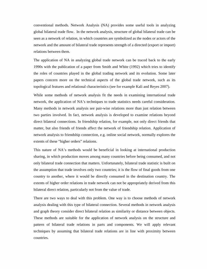
Figure 2a, and 2b present the maximum spanning tree graph for trade in parts and
components in 1985 and 2005 respectively. Value of the MST, which means the value of
trade covered by the most important bilateral trade link of these countries, is as high as 91%
and 96% of the total export in parts and components, for 1985 and 2005 respectively. Only
less than 9% and 4% of trade in those products take place, respectively for 1985 and 2005,
as non-MST bilateral relations – bilateral trade connections that are dropped and not shown
in the graphs. From technical point of view, these numbers suggest that the graphs
successfully cover important bilateral trade links. From economic point of view, the value

indicates high concentration of parts and components trade in the most important relations
only.
Both structures of trade relation in 1985 and 2005 expose a tendency of hub and spoke
relations between countries. This is in line with previous suggestions from the distribution
of degree and strength of vertices (VD and VS). There are several countries which serve as
hubs of the trade network, through which other countries are connected to the entire
network. USA and Germany are among the most important countries in the trade network
both for 1985 and 2005. Other countries include Japan, which serve as a hub for many East
Asian countries in 1985, France, which connect many Middle East and African countries,
and also UK.

Figure 2.a. MST Graph of Trade in Parts and Components 1985
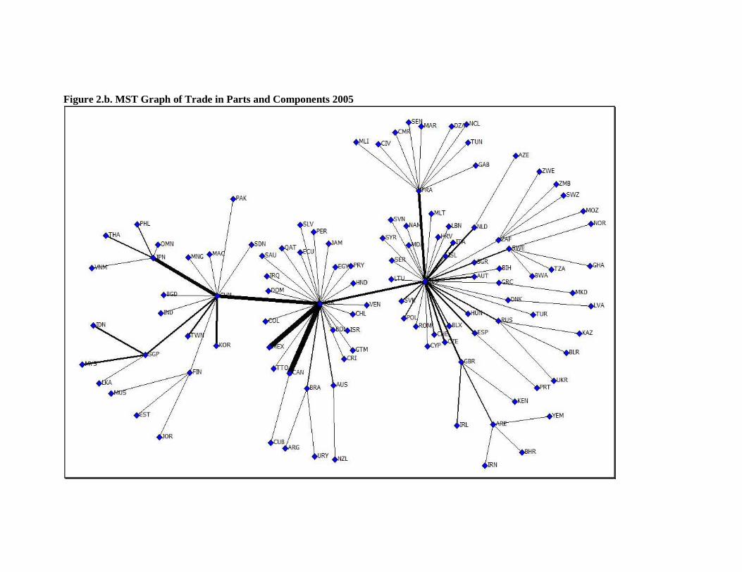
Figure 2.b. MST Graph of Trade in Parts and Components 2005

The position and role of some other countries also change during the period of observation.
While United Kingdom maintain its position as a hub for 2005, the importance of this
country as a bridge to the network diminishes as less country partners become connected
directly. Brazil has also emerged as a sub-hub to connect several other countries to the
network in 2005. Table 3 provide more detail description on the structure of MST for 1985
and 2005 by presenting 10 most important countries as hubs of the network, along with the
number of direct partners and the trade value. It is clear from the table that not only some
countries have become more important in the last two decades in the network of trade in
parts and components, but also some countries have lost their importance.
Table 3. MST of Trade in Parts and Components: A Comparison
Country No. of Partners Value of Trade Country No. of Partners Value of TradeUSA 37 31,168,432 Germany 33 81,632,456 UK 18 3,234,154 USA 29 106,901,954 Germany 15 9,160,420 France 11 13,111,647 France 9 2,655,493 China 8 59,813,866 CSK 5 115,789 UK 8 10,118,576 Japan 3 5,589,308 Japan 5 24,197,890 Sweden 3 1,027,320 South Africa 5 1,192,589 Hong Kong 3 680,804 UAE 5 991,596 Yugoslavia 3 187,205 Singapore 4 17,546,223 Mexico 2 2,790,095 Rusia 4 1,242,980
20051985
With regard to East Asian countries the two MST graphs also show that connections among
countries in the region have become stronger during the last two decades. While for 1985,
the graph shows heavy dependence of the regions to the US, where 6 out of 12 countries
place the US as their important partner, the graph for 2005 display stronger role and position
of some big East Asian countries to serve as hub in parts and components trade for other
countries in the region.
High value of global trade’s MST and evidence of hub and spoke structure of the network
suggest highly concentration of production sharing activities in several countries. The result
indicates that those countries serving as hubs play the most important role in shaping up the
global network of production. Moreover, with only less than 4% of global trade in parts and
components takes place between those spoke nations and their non-hubs partners, the
practice of production fragmentation tends to happen between countries belong to the same
group. These groups consist of one country as a hub and many other countries as spokes.
We take a look at this grouping tendency in more detail in the next sub-section. In the
meantime we explore more the non-MST relations of the global trade network.

More on the Structure and Pattern of Trade Despite its clarity and simplicity, our MST graphs, by focusing only on the most important
connection between pair of countries, basically throw away some other information that
might be useful. Therefore it is quite informative to complement the MST graph with other
less important trade relation between countries. Figure 2.c present MST graph for 2005
complemented with four largest bilateral trade relations of each country.
The graph clearly indicates that beside the MST relation, there are many other important
bilateral trade links dropped by focusing only on the most important ones. The most
noticeable one is the connection between US, Japan and China, which form a triangle trade
relation. Another structural characteristic that can be observed is the tendency of countries
which share the same hub to connect intensively to each other.
Although trade relations between countries belong to different hub are not rare, these are
less prevalent than trade link between country pairs sharing the same hub. In fact if the
bilateral trade relations in the graph are reduced to the two largest, instead of the four
largest, most visible links belong only to countries sharing the same hub. This confirms our
previous notion about the prevalence of production sharing between countries in the same
group.
Given the description on the structure and pattern of trade using the MST diagram, one
might ask whether such structure and pattern are uniquely observed in the trade network of
parts and components or if they also apply to trade network in general. Figure 2.d presents
maximum spanning tree graph for the network of total trade in 2005. The structure of hub
and spoke is also observed for this network, with USA and Germany as two important
countries.
However, there are several differences in the structure and pattern of total trade network and
trade in parts and components that can be observed from the MST graph, particularly in the
position of countries in the network. The most obvious one is the position of China which in
the total trade network ranks as the 9th most important country by having only five other
countries directly links their largest trade relation with this country, compare to being the
third most important ones in parts and components. China’s position is lower than Japan,
which serves as a hub for 10 countries. Other countries that do not serve as important hubs
in the network of parts and components, such as Italy and Brazil, turn out to become more
important in total trade network.

Figure 2.c. MST Graph of 2005 plus the Second Largest Bilateral Trade Relations

Figure 2.d. MST Graph of Total Trade Network in 2005

In short, the MST graphs of trade network in parts and components employed in this section
identify clearly the hub and spokes structure of network with only several countries play
important role. However, the structure is less clear in East Asia where trade relations outside
the hub and spokes links are also quite important. The importance of hub and spoke type of
relations indicates that trade and production activities spread across countries within the
same group. Furthermore, the graphs suggest that this grouping may follow geographical
location of the countries. In order to see further the pattern of bilateral trade in parts and
components with regards to this grouping, we will use other network analysis and statistical
techniques in the next sub-section.
2.3 Pattern of Trade: Mapping the Network The proposition that international production network is a regional phenomena has been
widely accepted9. Many studies in fact examine the so-called vertical fragmentation of
production by focusing intensively on the regional tendency of the phenomena and accept
the regionalization as a factual characteristic of the network. But rarely this tendency is
examined without a-priory assumption about the countries grouping. Here using some
statistical methods commonly employed in network analysis, we examine whether the
pattern of global trade in parts and component follows geographical distinction of economic
regions. We try to visualize the network of trade based on the consideration explained
earlier that the bilateral trade relations between countries is seen equivalent to proximity.
After that we use the results of the analysis to see the pattern of integration.
Multidimensional Scaling One common approach for visualization of network is known as the multidimensional
scaling (MDS). This method is part of a larger statistical technique loosely known as
dimensional reduction or ordination. The basic idea of this analysis is to “reduce”
dimensions of the data in order to provide clearer view on its pattern, usually in two
dimensions (Scott 2007). By mapping the connection profiles between countries in two
dimensional data, MDS provides coordinate of each node, in our case is the country of
origins, which can be plotted in a normal Cartesian system. Unlike other methods of
dimensional reduction, such as principal component analysis, techniques developed in MDS
do not require the linearity of data.
9 Arndt (2002) provides conceptual explanation on the regionalization of production sharing by arguing that lower trade barrier allow producers to exploit the difference in factor endowment. Many empirical and descriptive studies are also based on this consideration (see the next footnote)

Let the vertices of graph G(V,E,w) are seen as objects V and the symmetric weight wrs
become the dissimilarity measure between object r and s, δrs=- wrs. With this definition, the
greater the weight the closer the distance is between the two nodes. An arbitrary mapping of
φ from V to X, a set of points in a Euclidean space, is also defined. The distance between
points of xr and xs is given by drs. The aim of multidimensional scaling analysis, in general,
is to find a mapping φ for which drs is approximately equal to a monotonic transformation of
dissimilarity between the vertices f(δrs) following the minimization of certain objective
function also known as stress function.
So, in the implementation of an MDS technique, there are two important choices need to
make: the transformation of f(δrs) and the stress function. In the so-called metric or scale
MDS, f(δrs) is the dissimilarity measure itself; therefore distance between points in
Euclidean space is associated with the original data of dissimilarity. In the non-metric or
interval MDS, the disparities measure ̂drs= f(δrs) is a monotonic transformation such that it
follows either
rsrspqrs dd ˆˆ ≤⇒< δδ (weak monotonicity) or rsrspqrs dd ˆˆ <⇒< δδ (strong monotonicity).
Here, what matters is not the original measure of dissimilarity δrs, but rather the rank of the
objects V based on their dissimilarity measure.
The stress function is the measure of fitness of the estimation. By minimising the function,
which is basically variant of the difference between drs and f(δrs), the best configuration of X
representing the vertices is attained. One of the most commonly used stress function is
( )2
2
,
ˆ
rs
srrsrs
d
dd
S∑ −
=
which is minimized with respect to drs, and also with respect to ̂drs using an isotonic
regression. The minimization of S is a complex operation that can be achieved only by using
computing algorithm (Cox and Cox 2001). Numerous algorithms have been developed to
find better result of MDS. The analysis that follows makes use of an algorithm called
MiniSSA, which is based on non-metric MDS with the above description of stress function.

Map of Trade Relations and Regionalization The result of MDS analysis of trade in parts and components for the period of 1985 and
2005 are represented in Figure 3a and Figure 3b. In both graphs the position of each country
in our dataset relative to others corresponds to the representative point. Bear in mind that
while in a MDS graph, location of a particular node relative to others represents the distance
between nodes, the dimensions itself (horizontal and vertical axes) bears less significance.
What matters is the relative position. Our MDS mappings of trade in parts and components
come with the stress function of 0.200 and 0216 in 1985 and 2005 respectively. This is far
from perfect mapping, which is quite understandable considering the complexity of trade
relation between countries and the difficulties of reducing big relational data (98 countries
in 1985 and 114 countries in 2005) into two dimensional vectors.
One of interesting feature we can observe from mapping of countries based on their trade
connection is the tendency of grouping. Our previous MST analysis reveals that the
structure of global trade in parts and components tends to be circulated within groups of
country. The MDS map in figure 3a and 3b compare the location of countries based on trade
relations and their geographical location by color-coding the nodes following regional
grouping described in Appendix B. This is useful to see if countries groupings show a
resemblance to geographical regions.
We can see in Figure 3a, that regionalization as it is usually hypothesized finds less
evidence in the MDS analysis of trade network in 1985. Some countries which are
geographically closed to each other are connected quite significantly, such as the US and
Canada, or some developed European countries. But beyond those few countries, most are
not mapped according to their geographical location.
Most noted is the lack of existence of the Factory Asia. Japan, as the center of the region, is
closer to the US and Canada than to many other countries in the region. Except for newly
industrialized economies (NIEs) of this region, such as Hong Kong, Singapore and Korea,
countries in the region are a little bit far from the centre of the map. Even for those NIEs,
attachment to the US, probably as the main important market, are stronger than to other
countries in the region. The rest of East Asian countries are scattered around, with no clear
sign of clustering among them, with China and Vietnam located at the other end of the map.

Figure 3.a. MDS Map of Parts and Components in 1985

Similar pattern can be observed in other geographical groupings. The regionalization of
European countries is also limited to some industrialized western European countries. Other
European countries, such as Portugal and Ireland are yet fully integrated to the network of
machinery production in the region. Eastern European countries are far away from the
western European countries, indicating no significance trade relations between the two
regions. Nor there is visible sign of clustering among the Eastern block countries. While
most Latin American countries are located in the same part of the map, they are relatively
far from each other indicating low intensity of trade in parts and components.
A totally different picture can be observed in Figure 3b, which describes the situation in
2005. Regionalization of trade in parts and components is more prevalent in this picture.
East Asian countries seem to be more clustered during this time compare to the situation in
1985, with some more developed and developing countries are located closed to each other,
indicating strong trade relation among them. Note that European and East Asian countries
are located next to each other, with US and Canada being part of the core of the map.
We can also observe integration in other parts of the world in line with geographical
location of the countries. Countries in Central and Eastern Europe tend to be clustered in the
same part of the map, while some countries, such as Czech Republic, Poland and Hungary,
are virtually integrated into the western part of the continent. To a lesser extent, Latin
America countries are closely located to each other, particularly Brazil, Mexico and
Argentina. Other regional groupings such as Africa and Middle East, while demonstrating
trend of greater integration, are still located far from each other due to low intensity of trade
relations in parts and components among those countries.
The results from MDS maps of trade in parts and components present some interesting
features of global production sharing that is difficult to see using more conventional
descriptive techniques. Regionalization of production fragmentation, which is normally only
assumed in many studies, can be noticeably observed with the application of this technique.
While mapping trade relation in parts and components provides clear visualization on the
pattern of trade and the tendency of regionalization, it is useful to see this regional
indication using more appropriate techniques to supplement our ongoing exploration on
global production sharing.

Figure 3.b. MDS Map of Parts and Components in 2005

Further Notes on Regionalization of Trade: Cluster Analysis One method that complements the application of multidimensional scaling is clustering
analysis. Clustering is the process of organizing a set of data into groups in such a way that
observations within a group are more similar to each other than they are to observations
belonging to a different cluster (Martinez and Martinez, 2005). Although this type of
analysis is not normally considered as part of network analysis, we employ some techniques
to present a clear cut analysis on regionalization of production sharing.
In this paper, hierarchical clustering method will be applied to the results of
multidimensional scaling from previous section to see the degree of association between
regionalization of trade pattern and geographical distribution. Hierarchical clustering is a
simple agglomerative algorithm based on a set of nested partitions. Given a set of V objects
with v×v distance matrix D={drs}, where its elements is the Euclidean distance between
countries r and s from our previous multidimensional scaling results, hierarchical clustering
runs from v number of clusters each containing a single object to a single cluster containing
all objects.
The goal in hierarchical clustering is to link the two closest clusters at each stage of the
process. At the first stage, two closest clusters are simply two closest objects, where the
distance between them is minimum. However we need to define the distance between
clusters at the next stages of clustering iteration. In this analysis we follow Complete
method in which distance between two clusters p and q is described as the furthest distance
between objects in those two clusters.
The most common way to visualize the result of hierarchical clustering is by visualizing it
using a dendrogram. A dendrogram is a tree diagram which final leaves represent all
individual objects evaluated. Each object is connected to the other by sub-branches of the
tree, arranged in a hierarchical or nested manner. The position of each object in a
dendrogram determines its relevance to other objects. Objects that belong to the same sub-
branch of the tree are relatively closer than the ones belong to different sub-branches. In our
exercise, the objects are all nations in the sample. Their positions in the nested-tree
dendrogram determine how countries can be clustered together.
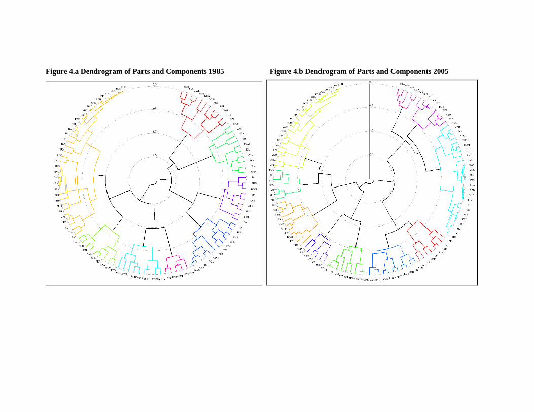
Figure 4.a Dendrogram of Parts and Components 1985 Figure 4.b Dendrogram of Parts and Components 2005

Figure 4.a and 4.b present the results of our clustering exercise. As can be seen in the
dendrogram for 2005, the leaves for China (CHN) and USA, for example, are closely
positioned and belong to the same farthest sub-branch, indicating strong relation in trade of
parts and components between the two countries. China and USA are also relatively closed
to Korea (KOR) and Canada (CAN) as they belong to the same sub-branches, despite at
higher level. Interestingly, China is relatively far from Japan since they share sub-branches
of the dendrogram at relatively higher level.
This dendrogram serves as a basis for further analysis which leads to grouping of countries.
There are several common methods for grouping of objects based on information in the
dendrogram. The simplest one is to get a group based on certain level of sub-branches.
Countries belong to, for instance, the 4th sub-branches from the center are grouped together.
Most common way is to classified countries based on the distance between the center and
sub-branches.
The normalized distance is represented in the dendrograms by radian circles in the graph
with certain values attached. In dendrogram of 2005, if we have a cut-off point of less than
0.5, most East Asian countries, together with Canada and USA will be grouped together.
Color-coding of sub-branches in our dendrograms is based on cut-off point of 1. Countries
with the same color belong to the same group. This results to countries being grouped
according to the color-coding.
More proper way to classify objects is by deciding certain number of groups to which all
objects would belong to. Based on the distance between leafs – a bit different than distance
from the center previously used for color-coding the leaf - each country can then be placed
in a particular group. A rectangle tree map (Wills 1998) is a convenient way to present and
evaluate clusters with their associated members. Figure 5.a and 5.b present tree maps for
countries based on trade in parts and components for 1985 and 2005 in 10 groups.10
10 The original tree map normally uses color-coding to see the clustering of objects by comparing to certain criteria. Here, we just spell out the grouping of countries and do the comparison using different method. Selection of 10 groups is basically arbitrary although one can use more formal method to choose the appropriate number of groups.

Figure 5.a Treemap of Countries in 1985
Figure 5.b Treemap of Countries in 2005

As we can see, the grouping of countries follows loosely regional classification commonly
recognized, although here and there, there are some exceptions. It is interesting to see how
far this grouping resembles regional classification, and how different the situation is in 1985
and 2005. Following the results, we can see that countries in the same geographical regions
are more inclined to be grouped together. This grouping is even more observable in 2005.
East Asian and North American countries are closer recently than in the previous period.
Latin American countries also belong to the same group while they are rather scattered in
1985. Similar pattern of regionalization as it is observed in our previous network analysis
are more apparent using this cluster analysis. To provide clear-cut examination, we can
compare how far the grouping from clustering analysis bears resemblances to geographical
regions.
One way to see it is by looking at adjusted Rand index (RIA) which measures the similarity
between classifications. The index indicates the proportion of objects that agree between
two groupings, which is calculated as the ratio of the difference between numbers of pairs in
agreement and its expected value (N) with the difference between maximum numbers of
pairs in agreement and its expected value (D). Given two partitions of G1 and G2, each has p
and q number of groups, RIA is defined as
−
−
==
∑∑∑∑
∑∑∑
2
22
2
22
2
22
2
....
..
n
nnnn
n
nn
n
D
NRI
q
q
p
p
q
q
p
p
q
q
p
p
pq
pq
A
where npq is the number of objects placed into group p in G1 and q in G2, while np. and n.q
denote the sum of npq with respect to each partition. Therefore RIA is a standardized measure
that gives a value zero when the groupings are randomly placed and one if they perfectly
match each other.
We compare the groupings of countries presented in Figure 5.a and 5.b with respect to
common regional classification described in Appendix B. The adjusted Rand index for 1985
is 0.308, indicating relatively weak correspondence between regional groupings and
groupings based on trade relation in that period. The index is also still low in 2005, which is

only 0.46411. Roughly speaking, this index shows that almost half of the nations in our
sample fall into the same category of their geographical regions in 2005, an increase from
only 30% of them in 1985. While the match between those two grouping are still low, there
is a tendency of higher regionalization in trade relations.
The application of clustering analysis supports the indications we obtained in the previous
section. Global trade in parts and components tends to occur between nations belong to the
same region and it becomes stronger over the period of observation. Clustering also
provides some information on the extent of this regionalization.
How Different 1985 and 2005? Globalization vs Regionalization The notion that trade relation, particularly in parts and components tends to be increasingly
regionalized is quite noticeable in our preceding analysis. The maximum spanning trees for
trade network in parts and components show that the connection mostly takes place among a
particular hub country and its spoke, indicating grouping in global production sharing
practice. Visual observation with the map of multidimensional scaling analysis shows that
countries tend to have more trade relation with their neighbours, in particular for East Asia,
European and Latin America economies. In all those regions, one big and important country
performs as the hub and its smaller neighbours become the spokes. This regional tendency is
further confirmed by clustering analysis, which clearly outlines intensification of regional
activities in the production fragmentation.
Rand index of clustering analysis shows that the grouping of countries based on trade
relations in 2005 follows regional classification more closely than in 1985. However, it does
not say much on to what extent the pattern of regionalization has changed during twenty
years of observation. Once again, we apply the MDS analysis to see the pattern of trade in
parts and components for two observation periods of 1985 and 2005. Rather than having
two maps separately presenting the two periods, the comparison can be done on the same
map. The comparison cannot be done directly by putting the MDS coordinates of the two
periods directly, since both maps are produced on different spaces: 1985 trade relations and
2005 trade relations. In order to do the comparison, both maps need to be translated,
rescaled, and rotated to place the countries in the same space.
11 Alternatively, we can also compare the clustering outcome from trade relation and clustering based on geographical distance of countries. The index for this comparison is 0.26 in 1985 and 0.39 in 2005.

Figure 6. MDS Map of Parts and Components in 1985 and 2005

A statistical analysis known as Procrustes provides general transformation of shapes into a
different space. The application of Procrustes transformation to the MDS maps of trade
relation is presented in Figure 612. The map places the countries on the same two
dimensional space describing trade relation in parts and components for the period of 1985
and 2005 together to allow direct comparison. Nodes with country label 1 denotes the
position of each country in 1985, while nodes with label 2, represent the position in 2005.
To make the map more readable, we only show positions for 50 countries in Figure 6.
Again, the tendency of regionalization is quite noticeable. Countries in East Asia, Europe
and Latin America are closer to each other in 2005, and tend to cluster following
geographical regions. However, there is also a tendency that all countries to become closer
as a whole. While countries have more intensive trade relations with their neighbours, they
also increase their trade with the rest of the world. The MDS map shows that the groups
have a tendency to move closer to the center of the map, indicating more intensive relations
between countries from other different groups. The result of this examination suggests that
while the development of production network of machinery has taken place at regional
level, it also has occurred at the more global level.
In summary, our exercise in this section using statistical methods and techniques borrowed
from network analysis and graph theory presents some interesting indication. Following the
hub and spoke structure of trade network, trade relations tend to be concentrated to several
important nations. These countries play important roles in building production sharing
network among their group of nations. Further analysis reveals that this grouping follows
geographical regions, and becomes stronger in the recent time. However, in addition to
regionalization, there is also a tendency towards more globalization as each region becomes
more actively connected to others. To complement the analysis on trade network, we now
turn to information provided by input-output tables in the next section.
3 Beyond Trade Data: The Network of Production Analysis in the previous section describes several features of global production sharing by
looking at trade data on parts and components using various tools from network analysis and
graph theory. Using trade statistics to examine production fragmentation suffer the risk to
12 There are also some attempts to develop dynamic MDS procedure, in which time dimension is taken into account directly in the formation of the map, instead of doing it separately. However, Procrustes analysis offers much simpler procedure with reasonably accurate outcomes (Cox and Cox 2001).

overestimate its importance due to double counting in the construction of the data as
discussed in the introduction section. Some attempts have come up with more
comprehensive measure by combining information from international trade data and table of
input output of production. Hummels, Ishii and Yi (2001) pioneered for this approach. In
this section, we follow their lead in using input output tables as a complement to trade
statistics. The goal is to reveal more features – especially the network features – of
international production sharing.
The method developed in this paper differs from current methods of combining trade
statistics and input output tables in which we take into account the network properties of
global production sharing. Existing methods mostly measure production sharing activities of
a country as the role of imports to production and exports. For example, the parts of US
exports (both final and intermediates) that comes from its intermediate imports; the basic
approach is to calculate the import-contents of US exports. In other words, it focuses on
triangular linkages between domestic production, imports and exports of a single country.
Although this approach can be applied to a lot of number of countries, the single-country
perspective misses the higher order network linkages. For example, the US imports of parts
and components from other countries is likely to contain some sub-parts and components
from the US manufacturers itself. The standard way would not recognise that some of the
US imports of intermediates actually contain US value added. There are many other
examples of network features that the focus on triangle linkages misses. In short, the
standard approach does not capture effects of the whole global network of production
sharing to countries in question. By putting it in a network perspective, our proposed
method tries to capture such aspect more completely.
In order to take advantage of the new analysis, we need to transform information from
input-output tables, together with trade data, to represent international linkage of production
process. But before going on to the core of the analysis, we first examine some indicators
using current procedures to enable comparison with the proposed procedure.
The input-output tables used in this section come from the OECD IO tables. These tables
provide harmonized information on production structure of 20 good sectors (and 17 service
sectors) based on the aggregation of 2 digits International Standard Industrial Classification
(ISIC) version 3. It includes information on input-output structure of production for 7

machinery products13. There are IO tables for 42 countries of OECD and several emerging
countries available every 5 years. To complement the information from OECD IO tables, we
also collect three more IO tables of East Asian countries, which are not available from the
OECD database14.
3.1 Some Indicators of Production Unbundling Before explaining our new methods, we apply standard methods to the IO tables in order to
provide the basis of comparison between the standard methods and our new methods.
Specifically, we calculate indicators based on methodology proposed by Hummels et al.
(2001), i.e. the use of imported inputs to produce goods that are afterwards exported. These
indicators are applied to look at the importance of international production sharing in the
machinery sector.
Import Contents of Exports The first indicator is the value of import contents of exports, also known as vertical
specialization index in Hummels et al. (2001). This indicator is computed by taking into
account the share of imported inputs, directly and indirectly, used in production, including
for exports. The result is the value of exports coming from imports. The formula can be
written as
kr
kr
kr XcIC =
Where
1)(' −−∈ dm CICnkrc
krX is exports of product k from country r, Cm and Cd are the coefficient matrices imported
and domestic intermediate input respectively derived from the input-output table of r, while
n is a column vector with elements of zeros and ones indicating certain intermediate inputs
to be included in the calculation. This column vector acts as the summation vector of the
share of intermediate inputs in the production. In our calculation, elements of the vector are
kept to be zero except for the ones related to the machinery sectors.
13 The seven machinery sectors include general machinery, electrical machinery, office machinery, motor vehicle, other transport, precision machinery and telecommunication. 14 We complement the data with IO tables from Malaysia, Singapore and Thailand. Fortunately, machinery sectors are relatively well defined and classified quite uniformly in various countries IO tables. It makes the harmonization attempts for those tables are relatively easier.

By assuming that the production structure of exports is the same as the production structure
of domestic consumption, we can use the calculated coefficient of krc , combined with the
value of exports from trade statistics, to compute imports value of country r embedded in its
exports for each product k. Notice that these IC measures are basically measures of a single
node’s involvement in the entire network, i.e. imports from all nations are summed, and
exports to all nations are summed.
Figure 7 presents the distributions of import contents for each seven machinery sector. As
we can see, the import contents of each product differ significantly across country.
Electronic sector, which include electrical, office and telecommunication, are the most
varied sectors in terms of import contents. They are also among the most import intensive
sectors, other than motor vehicle.
Figure 7. Import Contents of Production across Countries
0.2
.4.6
.8
Electrical Machinery General Machinery Motor Vehicle Office Machinery Other Transport Precision Machinery Telecommunication
1995 cont_mach 2000 cont_mach 2005 cont_mach
Figure 8 presents the share of import contents of exports (IC) for machinery products in
1995 and 2005 for 45 countries in the sample. This is calculated as weighted average of
import contents of exports for each of seven machinery products, with export value as the
weight. Therefore there are two factors that can explain the change of import contents
during the ten years period, which are the production structure of each of seven machinery
sectors and the importance of each sector in exports of machinery. Bigger trade in one of the

machinery products that consumes more imported inputs would result in higher share of
import contents of the machinery.
Figure 8. Import Contents of Production across Countries
ARG
AUS
AUT
BEL
BRA
CAN
CHE
CHL
CHN
CZE
DEUDNK
ESP
EST
FIN
FRA
GBR
GRC
HUN
IDN
IND
IRL
ITA
JPN
KOR
MEX
MYS
NLD
NZL
PHL
POL
PRT
ROM
RUS
SGP
SVK
SVN
SWE
THA
TUR
TWN
USA
VNM
ZAF
0
0.1
0.2
0.3
0.4
0.5
0.6
0.7
0 0.1 0.2 0.3 0.4 0.5 0.6 0.7
Import Contents of Exports 2005
Import Contents of Exports 1995
Re-exporting Share and Production Integration As mentioned above, the import contents of exports is only part of the story. The other part
of the story is related to the share of imports from other countries that would be further
processed for exports. This indicator RX, which stands for re-exporting index, shows the
importance of a particular country in the network. Higher share of imports that would be
further exported indicates higher integration of the country into global production network.
A country that uses most of its imports to produce exports can be considered as an important
link in the network of production sharing, while a country that only uses a small share of its
imports in its exports to be less influential.
kr
krk
rkr M
XICRX =
Furthermore, the RX indicator can be used to give a preview on network aspect of
production sharing. Network features of production sharing imply that parts of the exports
of a particular country o would be re-exported by its destination country r. When a country
o exports its products to country r, and country r embeds these imports in exports to other

nations, the global production network has enabled country o to export to the rest of the
world, but indirectly.
If a significant part of o’s exports goes to destinations with high RX, it is likely that a
significant share of the exports would be used for producing destination countries’ exports.
South East Asian countries, for example, are better connected to the global network since
their major destinations are China and Japan, which embed high shares of imports in their
exports (RX). This indicator of PI, stands for production integration, captures certain
network aspects of production sharing by looking the second-degree relations in trade and
production. Assuming that country r’ s share of imports embedded in its exports (RX) is
invariant to the origin of imports, then PI of nation o is simply a weighted average of its
destination’s RX and each market’s export share.
sample in thecountry :; RrRXX
XPI k
rr
r
kor
kork
o ∈=∑∑
Figure 9. Re-exporting Share of Imports (RX)
ARG
AUS
AUT
BEL
BRA
CAN
CHE
CHL
CHN
CZE
DEU
DNKESP
EST
FIN
FRA GBR
GRC
HUN
IDN
IND
IRL
ITA
JPN
KOR
MEX
MYS
NLD
NZL
PHL
POL
PRT
ROMRUS
SGP
SVK
SVN
SWE
THA
TUR
TWN
USAVNM
ZAF
0
0.1
0.2
0.3
0.4
0.5
0.6
0.7
0 0.1 0.2 0.3 0.4 0.5 0.6
Re-exporting (RX) Share 2005
Re-exporting (RX) Share 1995
Figure 9 presents the share of imports re-exported further of 45 countries for 1995 and 2005.
The noticeable feature from the graph is that most countries only re-export further small
parts of their machinery imports. Here we can see that the biggest part of the imports remain

to in the domestic economy. However, there clearly is an upwards trend of this re-exporting
share for most countries.
Figure 10 describes how well connected countries in East Asia and USA are to the
international network of production sharing. In general, more than 10% exports of these
countries are embedded to their partner’s exports. China and some other countries are
clearly becoming more integrated, while some others slightly reduce their interconnections.
Figure 10. East Asia’s Integration to International Production Sharing Network (NI)
0
0.05
0.1
0.15
0.2
0.25
0.3
CHN IDN JPN KOR MYS PHL SGP THA TWN EA USA
1995
2000
2005
Some indicators explained and calculated above give some indications on the patterns of
production sharing. The calculation of import contents of exports (IC) can give indication of
how important production sharing is in a particular country. Moreover, the indicator can be
used to see how well the country has been integrated into the global production network by
looking at the extents to which its production is used by other countries.
However, as discussed above, they focus only on triangle linkages (a single nation’s
imported inputs, production and exports). IC index for country r, for example, only
measures effect of country r’s imports on its exports. Index for production integration (PI)
of country o, while take the analysis a bit further, is still limited to examine the effect of o’s
production on production activities in its destination countries. It is difficult to see
production linkages beyond this triangular relation. This might lead to a misperception of
the true nature of the production network.

Indicators of IC and RX for our sample of countries, for instance, might lead to conclusion
that countries like Philippines or Thailand are better connected to global production sharing
network than China and Japan (Figure 8 and 9). A priori, such a conclusion is not credible
given the abundant anecdotal evidence15. The two indicators basically tell us that production
sharing is important and might shape performance of the countries’ trade and production.
They do not, however, tell us about how important and how well connected these countries
are in the global network.
While PI indication provides some aspects of the necessary information, it is focusing only
on triangle connections; it takes no account of effects from the rest of the network. As such,
it might lead to inaccurate conclusions. In East Asia, for instance, the indicator shows that
South East Asia countries seem to be more connected than their northern counterparts
(Figure 10). This is not in line with common proposition based on case studies and our
analysis of trade network in previous section. These shortcomings are what motivate our
search for a new procedure that does not only offer better way in calculating the indicators,
but also better perspective to approach the problem.
The next sub-section offers new angle in looking at production sharing with the help of
input output tables. The new procedure enables us to see the contribution and role of a
particular country, not only to its direct partners, but also to the whole global network of
production sharing.
3.2 New Measure of International Production Sharing As discussed earlier in the introduction section, the recent development of international
production sharing is a complex arrangement involving not only production process, but
also intensive logistics and cross-border transportation, as well as sophisticated coordination
and management systems. However, at the very basic form, this phenomenon is similar to
other economic activities, in which production flows from one place to another, where the
value of products is improved by further processing. The input-output table is basically
constructed to describe the flow of production across sectors in a single economy. In the
following, we look at the international production sharing activity as the flow of production
15 Some surveys of Japanese MNCs shows that their activities in China are much higher than their counterparts in ASEAN countries. See survey from METI available at http://www.meti.go.jp/english/statistics/tyo/kaigaizi/index.html, or from JBIC at http://www.jbic.go.jp/en/about/press/2010/1203-01/index.html

– but rather than describe flows across sector within a nation, we put emphasis on cross-
borders flow within a single sector.
Input-Output System of Network Flow The insight that economy can be visualized as a system similar to network flow model is not
new. In fact, the famous input output model shares many characteristics of network flow
model, where goods and services flows across sectors satisfying a set of constraint (Leontief
1974). Olsen (1992) demonstrates that both quantity and price model of economic input-
output resemble special cases of network flow problems commonly found in network of
transportation and network of electricity current.
A system of economic input-output can be described as a matrix which is equivalent to the
adjacency and weight matrix of a network. The basic form of input-output matrix normally
follows the description below.
=
021
21
222221
111211
j
iijii
j
j
fff
daaa
daaa
daaa
L
L
MMOMM
L
L
T =
0F
DA
Sub-matrix A in the IO system corresponds to cross-sectoral links of intermediate inputs,
where aij is the amount of products from sector i sold and used for further processing
activities in sector j. Sub-matrix D, with di as the elements, refers to final demand, where
products are sold and used for final consumption, while sub-matrix F, with elements fj refers
to primary factors used in the production sectors. The zero reflects the fact that the total
value of inputs equals the total value of output in a closed economy.
From a network flow perspective, the table represents a system of production, in which the
internal part of the system, A, receives flow of primary inputs, F, from the environment and
giving back D to the environment. In formal terms of network flow model, the intermediate
input part of the table is known as internal flow of the network. Both primary factors and
final demand parts of the table are known as boundary flow, where economic activity flows
into and from the sectors in economy.
Using this concept of network flow, various techniques related to graph theory and network
analysis can be employed to examine the structure of an economy represented by an IO
table. Earlier works of this literature include Slater (1978) which employ maximum-flow
concept of network flow theory to examine the structure of US economy. More recent
papers including Muñiz et. al. (2010) examine core-periphery structure of European and
Spain economy using network analysis and an extension of cross-entropy method16, whilst
in the same spirit Blöchl et. al. (2010) examines the centrality of cross-sectoral relations in
OECD member countries.
The analysis that follows in this section shares the same perspective of the literature in
network and IO system, but with emphasis on international aspects. The international
linkage of production can be regarded as the flow of cross-border economic activities, not
only cross-sectoral flow as described in a domestic IO model. Therefore we need to extend
the information from IO by combining it with trade statistics.
Stochastic Process of Production Flow By seeing international production flow as a
network flow between countries, equivalent to
cross-sectoral flow in IO model, in principle we
should be able to follow the path of production
flow between countries. Referring to the diagram
of international production flow on the right, we
should be able to follow what happens to one
dollar value produced in machinery sector in
country A: whether it is consumed domestically as
final demand (D), exported to B, or exported to D.
On its way through the international network of
production, that one dollar value can be improved
by having more inputs (O) from other production sectors and primary factors. We should
also be able to follow even further the path of its travel until it reach a destination where it
would be disbursed out of the system as final product (D). Information from this analysis
can then be used to provide useful information on several features of production sharing,
e.g. to see country’s importance and role in the international value chain or to calculate its
value added contribution.
16 Cross entropy method is a method widely used to update IO table based on limited or partial newer data. It works by minimizing the distance between a-priory information derived from newer data and existing IO table.
A
B
D
C
O
O
O
O
D
D
D
D
International Flow of Production
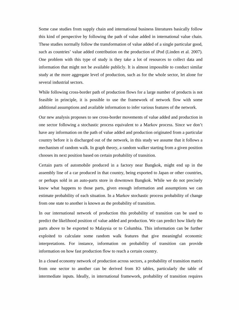
Some case studies from supply chain and international business literatures basically follow
this kind of perspective by following the path of value added in international value chain.
These studies normally follow the transformation of value added of a single particular good,
such as countries’ value added contribution on the production of iPod (Linden et al. 2007).
One problem with this type of study is they take a lot of resources to collect data and
information that might not be available publicly. It is almost impossible to conduct similar
study at the more aggregate level of production, such as for the whole sector, let alone for
several industrial sectors.
While following cross-border path of production flows for a large number of products is not
feasible in principle, it is possible to use the framework of network flow with some
additional assumptions and available information to infer various features of the network.
Our new analysis proposes to see cross-border movements of value added and production in
one sector following a stochastic process equivalent to a Markov process. Since we don’t
have any information on the path of value added and production originated from a particular
country before it is discharged out of the network, in this study we assume that it follows a
mechanism of random walk. In graph theory, a random walker starting from a given position
chooses its next position based on certain probability of transition.
Certain parts of automobile produced in a factory near Bangkok, might end up in the
assembly line of a car produced in that country, being exported to Japan or other countries,
or perhaps sold in an auto-parts store in downtown Bangkok. While we do not precisely
know what happens to those parts, given enough information and assumptions we can
estimate probability of each situation. In a Markov stochastic process probability of change
from one state to another is known as the probability of transition.
In our international network of production this probability of transition can be used to
predict the likelihood position of value added and production. We can predict how likely the
parts above to be exported to Malaysia or to Columbia. This information can be further
exploited to calculate some random walk features that give meaningful economic
interpretations. For instance, information on probability of transition can provide
information on how fast production flow to reach a certain country.
In a closed economy network of production across sectors, a probability of transition matrix
from one sector to another can be derived from IO tables, particularly the table of
intermediate inputs. Ideally, in international framework, probability of transition requires
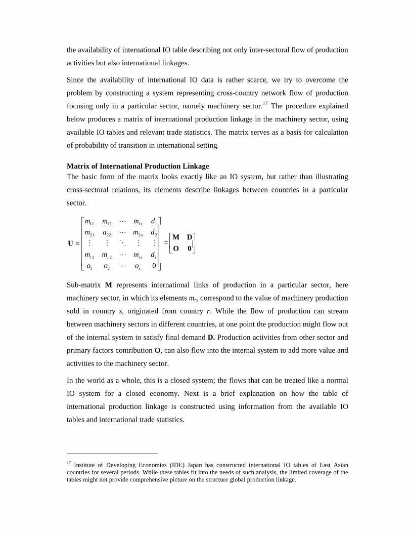
the availability of international IO table describing not only inter-sectoral flow of production
activities but also international linkages.
Since the availability of international IO data is rather scarce, we try to overcome the
problem by constructing a system representing cross-country network flow of production
focusing only in a particular sector, namely machinery sector.17 The procedure explained
below produces a matrix of international production linkage in the machinery sector, using
available IO tables and relevant trade statistics. The matrix serves as a basis for calculation
of probability of transition in international setting.
Matrix of International Production Linkage The basic form of the matrix looks exactly like an IO system, but rather than illustrating
cross-sectoral relations, its elements describe linkages between countries in a particular
sector.
=
021
21
222221
111211
s
rrsrr
s
s
ooo
dmmm
dmam
dmmm
L
L
MMOMM
L
L
U =
0O
DM
Sub-matrix M represents international links of production in a particular sector, here
machinery sector, in which its elements mrs correspond to the value of machinery production
sold in country s, originated from country r. While the flow of production can stream
between machinery sectors in different countries, at one point the production might flow out
of the internal system to satisfy final demand D. Production activities from other sector and
primary factors contribution O, can also flow into the internal system to add more value and
activities to the machinery sector.
In the world as a whole, this is a closed system; the flows that can be treated like a normal
IO system for a closed economy. Next is a brief explanation on how the table of
international production linkage is constructed using information from the available IO
tables and international trade statistics.
17 Institute of Developing Economies (IDE) Japan has constructed international IO tables of East Asian countries for several periods. While these tables fit into the needs of such analysis, the limited coverage of the tables might not provide comprehensive picture on the structure global production linkage.

The IO system described above has one main condition that characterizes its equilibrium:
the column sum of T is equal its row sums, emphasizing that supply of each sector’s
production equal to its demand.
DAιFAιt ' +=+= (1)
where ι denotes a vector with all elements of one and t is a vector of sums of rows or
columns.
While matrix T describes a closed economy system, most IO tables also contain some
information about exports and imports from the rest of the world. In an open economy
system, equilibrium condition of IO tables of country s can be represented as follow.
isi
si
i
sij
sj
j
sij
j
sij mxlafma −++=++ ∑∑∑ (2)
where aij and fj are the same as elements of closed-economy IO system. In this system
imported intermediate inputs mij is present, while final demand is decomposed into domestic
final demand l i, exported final xi and imported final mi.
Compiling elements of the table to describe activities in one sector of the economy resulting
to
si
si
si
i
sjiij
si
sj
j
sjiij
j
sjiij
sj
si
sjiij
sj
sjiij
sjiij
mxlad
fmao
wheredaoma
−++=
++=
+=++
∑
∑∑
≠
≠≠
===
,
,,
,,,
(3)
which illustrate activities in one sector only i=j , machinery sector in our case, for one
country s combined with information on how this sector relates to the same sector in the rest
of the world m, a composite input from another sector in that country o, and inputs from the
same sector in the country itself a.
The open economy part of this system, m, can be expanded to capture the source country of
intermediate input of machinery sector. Assuming that the composition of imported parts
and components used in machinery sector of country s follows the same pattern as its
imported parts and components M, imported intermediate inputs of machinery sector in s
originated from machinery sector in r, mrs, can be calculated as
sj
rsjrs
jsj
rsj
rsj M
Mmm == αα where (4)

Identity condition derived from a matrix U for country s is written as follow.
srrsj
sj
sj
sj
sj
r
srrsj
sj madaoma =≠ =+=++∑ ,, where (6)
The left hand side of the equation represents the column of the matrix of international
linkage for specific country s. Our matrix is constructed from 45 country specific IO tables
that compose 45 of its columns. The equilibrium condition of the whole matrix should take
the form as follow.
rj
s
rsj
sj
r
rsj dmom +=+ ∑∑ (5)
While the left hand side of (6) can be taken directly from (5), the right side hand needs some
adjustments particularly with regards to final demand dr. There are many methods in the
literature of input-output models developed to address such discrepancies18. However, since
most of proper methods require additional information that is beyond the scope of this
paper, not to mention that we basically focus on the use of intermediate input in machinery
sector, in this paper we use a simple approach to calibrate the system by treating final
demand of row r as a residual.
Using this new identity, we can construct a matrix representing cross-border production
linkage in a single sector. It takes form like an IO table as described in matrix U above. The
elements of the matrix describe production linkages for the global machinery sector, which
is basically total production of seven sub-sectors, between row countries and column
countries. Each element describes machinery products produced in the row country that are
used by machinery sector in the column country. The last row of the matrix captures the
contribution of factor of production and other sectors of production in each column country.
The last column presents row country’s net production consumed as final demand.
Similar to previous analysis on international trade network, conventional descriptive
analysis on bilateral relations of production linkage is difficult to carry, in part because it
involves quite big number of relations; in our case there are 2045 bilateral relations. The
matrix is also composed by “generated data” from IO tables and trade statistics, in which
18 The RAS biproportional adjustment method for updating IO table, for example, can be applied to come-up with a balance matrix of international linkage. However, we need to deal with different information on the sources of discrepancies

direct interpretation of its value might be subjected to many constraints19. Moreover, the
nature of connections described in this matrix perfectly suits the needs for analysis of
higher-order relations in a network, as previously discussed. Therefore in this paper, we use
information from the matrix to apply some new concepts and methods from network
analysis in order to examine some features of global production sharing.
3.3 Most Important Countries: Centrality Measures One of the recent developments in network analysis is the application of random walk
principle based on the stochastic process in examining structural characteristics of a
network. Random walk model of network assumes that a walker start from a particular
vertex and move to the adjacent vertices in order to reach a destination vertex. The choice of
which vertices the walker choose in the next move depends on a probability determined by
the associated weights. Newman (2004) uses the principle to propose some methods in
analyzing weighted networks, specifically in looking at centrality structure of the network
and sub-grouping of vertices.
Centrality Measures The concept of random walk fits nicely to capture various characteristics of the production
linkages described earlier. Production activity streamed from country r randomly chooses,
based on certain probability, the next country s in the network, where it might get additional
economic value, consumed directly as final product, or simply being transferred to another
country. In this section, we focus the application of random walk principle to see centrality
structure of the international production network.
We take advantage of information from the constructed matrix of international production
linkage, particularly the sub-matrix M which captures cross-border transition of production
in machinery sector. By dividing the elements of the matrix to its row sums, the probability
of cross-border transition can be acquired as the basis for further analysis.
MιMW 1))(( −= diag
The transition matrix W can be seen as a weighted network G(V, E, w) of international
production sharing, equivalent to the one for international trade previously discussed. But
19 As mentioned already, the matrix is constructed following a simple procedure due to availability of information. Interpreting elements of the matrix directly might not give much information and prone to inaccuracies. Even a carefully constructed IO table is rarely used to give direct information on the flow of production, but rather used for further analysis.
unlike the network of trade relations, the diagonal elements of W are not zero. These non-
zero diagonal elements indicate the importance of domestic machinery sector in supplying
parts and components for its own production. In network analysis term, this suggests the
existence of self-loop relations that has to be taken into consideration.
While it is possible to apply our earlier techniques to examine this network of production, its
flow characteristic opens up more possibilities than just considering the relations as
proximity, such as measuring the role and position of vertices in the network using the
concept of centrality.
The concept of node centrality is an important measure in network analysis, particularly
with regard to the network of social interaction. It provides information on how important a
node in the network and what role it plays. In our network of production, it can be
interpreted as the importance of each country in the global network of production sharing.
There are three main concepts of node centrality: degree centrality, closeness centrality and
betweenness centrality.
In this section we look at centrality of countries in the network of production using the
concept of closeness and betweenness based on random walk. By looking at node centrality
of the network, now we move from network level analysis in the previous section to
individual node analysis.
Closeness Centrality Closeness centrality indicates how close a vertex to other vertices in the network. It can be
regarded as an indicator of how long the flow from one vertex reaches other vertices in the
network. While the measure of closeness is clear in a distance metric like in our previous
analysis, there are various ways to define closeness in a non-distance graph such as the
international flow of production. Traditional method of network analysis normally defines
closeness in term of geodesic distance, which is basically the shortest path between two
vertices. However since the network of international production tends to be dense, geodesic
distance gives little insight to its structure. Based on random walk model, Noh and Rieger
(2004) suggests the use of mean first passage time (MFPT) to measure the distance between
vertices.
MFPT basically indicates how long on average does it take for a random walker to start
from r to reach a destination vertex s for the first time if it chooses the path randomly based

on certain probability distribution. It calculates the expected number of steps between the
two points
∑∞
=
=1
)(x
rsrs xPxMFPT
where )( rsxP is the probability to reach s from r at exactly x steps. While Noh and Rieger
(2004) proposes method to calculate MFPT for non-weighted network, Blöchl et. al. (2010)
modifies the method to accommodate calculation for weighted network. The probability can
be inferred from the elements of matrix W by prompting that it can be decomposed to the
probability of arriving at node t≠s after x-1 step and the probability of going from t to s in
the next step. Therefore
∑=−=t
tsrttsrtrs wPxPxP ω)1()1()(
where ωrt is the element of matrix (W-s)x-1, a modified of W without its s-th row and
column, and wts the element of W. In practice, the vector of FPT denoting MFPT from all
vertices in the network to reach a particular vertex s is calculated as follow.
ι)W(IFPT 1−−−= s where FPT is a vector size r×1 and ι a suitable vector of ones.
The random walk closeness centrality RWCC for vertex s is then the inverse of MFPT of the
vertex.
∑=
rrs
s MFPT
nRWCC
This centrality measure can be interpreted as a measure of efficiency of the flow to reach the
vertex. Country with high RWCC means that it can be reached by the flow of production
originated from anywhere easily, while low centrality indicates that the country is relatively
out of reach by the international production flow.
Betweenness Centrality Betweennes centrality defines different aspect of centrality, namely how important a vertex
lies on the paths between others. In other words it measures to what extent the importance of
a particular vertex to keep the network intact and to influence the flow. Conventional
betweenness centrality of a particular vertex is normally measured by counting how many
shortest path between other vertices go through it. However the density of international flow

of production and other characteristics require more attention. Newman (2004) proposes to
measure betweenness of vertex based on random walk model, by counting how often the
node is visited by the walker in its effort to travel between other vertices. Here we follow
Blöchl et. al. (2010) to calculate betweennes centrality for a network with self-loop nodes.
The betweenness centrality of node s is defined as the average number of times the node is
passed through by the flow originated from all nodes r, including s itself, to the destination
u≠r.
∑≠ −
=rur
rus
s nn
PTBC
, )1(
Where rusPT is the frequency of the flow passes through s, calculated based on transition
probabilities in W.
2
usrts
u
ursst
rus
wwPT
ϖϖ +=∑
where ursϖ is element of (I-W -u)
-1, and W-u transition probability
matrix W without u-th row and column.
3.4 Centrality Measures of Countries in Production Network Table 4 presents the result of centrality calculation based on random walk principle, both for
closeness and betweenness centrality. Given that IO tables, as the most important
component in constructing international production flow, are not available widely for the
whole range of countries over a long period of time, in this study we restrict the analysis to
only two period of time, 1995 and 2005. The analysis focuses on examining the role and
position of countries in international production flow and how it changes over period of
observation.
While there is a certain degree of similarity in the order of countries’ centrality based on the
two methods of estimation, the results also show differences due to the measurement of
different aspect of centrality as discussed earlier.
Closeness centrality of countries in the network of production sharing indicates how fast
production flow to reach a particular country. Higher closeness centrality of a country is
related to faster time needed for production flowing from other countries to reach it. In
2005, China, USA, Germany and Japan are among the countries with highest closeness
centrality measure. This suggests that those countries are easily reached by the production
flow originated from all other countries. With closeness centrality of 0.055 for USA and

China in 2005, we can figure out that it takes less than 18 steps on average for production of
parts and components in other countries to reach the two.
Table 4. Centrality Index of International Production Flow
Country 1995 2005 Rank in 1995 Country 1995 2005 Rank in 19951 USA 0.061 0.055 1 CHN 32.340 184.508 62 CHN 0.008 0.055 15 USA 137.097 175.014 13 DEU 0.044 0.045 2 JPN 102.788 112.271 24 JPN 0.031 0.028 3 DEU 66.956 105.967 45 KOR 0.024 0.022 4 KOR 94.424 69.666 36 FRA 0.021 0.019 6 SGP 20.949 56.187 97 TWN 0.014 0.018 9 FRA 35.476 47.820 58 MEX 0.006 0.017 18 TWN 18.164 36.832 119 SGP 0.023 0.016 5 CAN 19.170 34.891 10
10 GBR 0.019 0.016 7 BRA 25.584 34.573 711 CAN 0.017 0.016 8 GBR 24.485 27.999 812 ITA 0.013 0.013 10 ESP 14.888 27.112 1313 ESP 0.010 0.012 12 ITA 17.249 25.567 1214 MYS 0.011 0.010 11 MEX 5.508 25.542 2015 THA 0.005 0.009 20 MYS 9.753 22.049 1416 HUN 0.004 0.008 22 IND 2.643 16.971 2917 BEL 0.009 0.006 14 THA 3.992 15.203 2318 CZE 0.001 0.006 31 ZAF 2.717 13.009 2819 SWE 0.007 0.006 17 SWE 6.813 10.837 1820 BRA 0.005 0.006 19 HUN 2.977 9.711 2721 IRL 0.009 0.005 13 CZE 1.596 9.588 3322 NLD 0.007 0.005 16 BEL 9.203 9.198 1523 AUT 0.004 0.005 21 AUT 3.703 7.912 2424 PHL 0.003 0.005 23 NLD 8.237 7.677 1625 FIN 0.003 0.004 24 IRL 6.886 7.405 1726 POL 0.001 0.003 33 FIN 4.302 7.103 2227 IDN 0.003 0.003 25 POL 2.327 6.074 3128 PRT 0.003 0.003 27 PHL 2.471 5.987 3029 SVK 0.000 0.002 37 AUS 5.094 5.760 2130 AUS 0.003 0.002 26 IDN 6.596 5.380 1931 IND 0.001 0.002 34 PRT 3.341 3.899 2632 ZAF 0.001 0.002 36 SVK 0.523 3.726 4033 DNK 0.002 0.001 28 NOR 1.564 2.848 3434 TUR 0.001 0.001 32 DNK 2.091 2.676 3235 NOR 0.001 0.001 30 TUR 3.630 2.271 2536 ISR 0.001 0.001 29 ISR 1.391 1.543 3537 SVN 0.001 0.001 35 SVN 1.032 0.903 3638 EST 0.000 0.001 41 ROM 0.534 0.681 3939 ROM 0.000 0.001 38 EST 0.242 0.659 4140 GRC 0.000 0.000 40 GRC 0.646 0.477 3841 CHL 0.000 0.000 39 CHL 0.783 0.199 3742 LUX - 0.000 42 LUX - 0.104 42
Closeness Centrality Betweenness Centrality

The result of centrality estimation based on “closeness” concept is in line with the previous
analysis on the structure of trade in parts and components. In analysis of trade network, we
find that those countries play important roles in the network. Here, we also see that those
countries are closer than others that make them strategically located in the international
network of production sharing.
This measure of centrality can also be interpreted as the measure of how sensitive a
particular country to a shock started in other countries in the network. A supply shock that
occurs in any other countries would affect countries with higher centrality measure faster
and, over a period of time, more intensely than the ones with low measure. A positive
supply shock, such as an increase in final demand of machinery products, would provide
better opportunities to machinery sector in China than, say, other developing countries in
East Asia.
The reverse is also true. Negative supply shock would hurt machinery sector in China and
other countries with high centrality measure more considerably. This is in line with what
happened during the financial crisis of 2008/2009, where the machinery sector saw a very
significant drop in trade and production due to the fall of demand. Countries fully connected
in the international value chain of the sector, such as China and USA are affected faster and
more significantly than other less connected countries (Baldwin 2009).
Betweenness centrality measures the importance of a country by estimating how often that
particular country is visited by the flow of production streaming from a certain part of the
network on the way to other parts: higher number of visits indicates the country’s
importance as a “bridge” in the production network. This is a basic concept of betweenness
centrality. However, since the network of international production flow is a weighted
network and consists of domestic processing of the flow (self-loop), the centrality should
also considers how long the production flow is inside the country for processing before it
leaves. The stochastic random walk method used in this study takes that aspect into account:
larger weight of self-loop increases centrality of the country.
Similar pattern of centrality can be observed following the estimation of betweenness
centrality. USA, Japan and China are among the most central countries in the network. Like
analysis of trade network shows, those countries are among the most important hubs in the
global network of production linkages. High measure of betweeness centrality indicates that

if we drop one of these countries from the network, then it significantly disturb its structure
and interrupts global production sharing activities.
It is worth mentioning that China’s importance in the network is mostly due to its size of
domestic machinery sector. The calculation also considers the weight of domestic sector to
capture how long the production flow remain in the country, even though some countries
might serve as more important “bridge” in the network.
Table 4 also presents the centrality measures of the same countries in 1995. It is quite
obvious that there are some changes on the role and importance of those countries in
international production of machinery. In addition to China, that significantly has become
more important within ten years of observation, other countries, notably Mexico and several
Eastern European countries, have also become closer to other countries in the network. That
might be related to greater integration of those countries to other important countries in their
region: USA for the case of Mexico, Germany and France for Eastern Europe.
The network of international production flow in machinery is presented in Figure 11. In
order to simplify visualization of the network, only 5 highest production flows from each
country are presented in the graph. Each node denoting a country is placed according to
radial representation of a network based on the random walk centrality measures estimated
previously. Countries with higher centrality measure are located closer to the central of the
graph, while the lowest ones are the farthest. Figure 11.a shows the network of production
flow according to closeness centrality measure, while Figure 11.b follows betweenness
centrality.
In addition to the measures of centrality, countries in the network are also placed in relation
to their interactions in the production flow. Countries with higher flow coming in and out to
each other are located closer than countries with relatively low interaction. Width of the
links between countries in the graph also indicates the magnitude of the production flow
between them. In line with our finding in Section 2.3, countries tend to regionalize in this
network of production, where countries from the same geographical region (color-coded)
tend to be closed to each other. Comparing the graphs for 1995 and 2005 suggests that this
regionalization is more prevalence in 2005 than in the former decade.

Figure 11.a International Production Flow with Closeness Centrality Measures
1995 2005

Figure 11.b International Production Flow with Betweenness Centrality Measures
1995 2005

1
3.5 International Product Fragmentation in Other Sectors So far we have examined the pattern of international production sharing in parts and
components of machinery sector. Does the new production trend can only be observed in
machinery sector? To what extents are the importance of production sharing or international
flows of intermediate goods in other sectors? In order to answer these questions we employ
the centrality measure to examine international flow of production in some other sectors.
We choose to investigate agriculture sectors as a representation of resource intensive sectors
and textile as another manufacturing.
While both centrality measures normally provide indication on the position of vertices
within a particular network, the nature of closeness centrality can also present meaningful
suggestions towards the pattern of interaction between vertices in a particular network. It
then can be compared to the pattern of interaction in other network. Since RWCC is based
on calculation of MFPT, the (inverse of) centrality measure of country s can be interpreted
as the average number of steps needed by production flow to reach that country from other
parts of the world. The measure of certain countries in the networks of production of
different sectors can be compared to each other to see the differences in their pattern.
Table 5. Closeness Centrality of Other Sectors (Top 15 Countries)
USA 0.022 CHN 0.031 USA 0.055
CHN 0.009 ITA 0.024 CHN 0.055
JPN 0.005 USA 0.018 DEU 0.045
MEX 0.001 DEU 0.012 JPN 0.028
FRA 0.001 MEX 0.009 KOR 0.022
GBR 0.001 FRA 0.008 FRA 0.019
KOR 0.001 JPN 0.006 TWN 0.018
DEU 0.001 GBR 0.005 MEX 0.017
NLD 0.001 ESP 0.003 SGP 0.016
ITA 0.001 CAN 0.003 GBR 0.016
ESP 0.000 BEL 0.002 CAN 0.016
CAN 0.000 KOR 0.002 ITA 0.013
TWN 0.000 PRT 0.001 ESP 0.012
BEL 0.000 NLD 0.001 MYS 0.010SGP 0.000 ROM 0.001 THA 0.009
Agriculture Textiles Machinery
The closeness centrality of agriculture and textile sector, along with machinery, is presented
in Table 5. Only the centrality of top 15 countries is shown in the table.
From the table, it is quite clear that closeness centrality measure for countries according to
their production flow in the other two sectors are quite different than the measure of their

2
machinery sector’s production. Countries that are highly important in machinery might not
be that significant in the other sectors. We can also see that the magnitude of centrality is
quite different. For instance, the centrality index of the most important country in the
network of machinery production is 0.055, while in agriculture it is much smaller to 0.022,
and in textile 0.03.
This index can be interpreted as the speed of production flow to roam around in a particular
network. In machinery, it takes only around 18 steps in average for production flow to reach
USA, the most centered country, for the first time, while it takes almost 50 steps for
production flow in agriculture, and around 30 in textile sector. These indicate that
international production flow in other sector might not be as fast as the one in machinery
sector. It becomes even clearer when we compare less important countries in each network.
While in machinery sector, the top 5 countries tend to have similar centrality measure, in
agriculture the difference between the top country and the second one is very significant.
From this simple interpretation of the measure, we can figure out that production sharing in
two other sectors might not be as intensive as in machinery sector. Textile industry shows its
sign of the internalization of production, although still incomparable to what has taken place
in machinery.
4 Conclusion International production sharing has been emerging rapidly during several last decades. It
has attracted scholarly attention from various perspectives including from international trade
economists.
While there are many studies examining various trade features of this new phenomenon,
most studies are either focus on regional structure of production sharing or case studies of
several countries. Very little analysis has been done on the global pattern of bilateral trade in
parts and components. For this reason, the existing literature underplays the network aspect
of production sharing.
One obstacle in doing analysis at bilateral level of on a global data set is that it involves
considerable amount of data. Some help with this problem comes from network analysis
(NA) and graph theory, which provide some useful tools for extracting clear patterns from
masses of data. However, applying network analysis on trade data requires careful
consideration. Trade data typically focuses only on what NA calls first-order relationships
(e.g. Chinese exports to the US). Many methods in network analysis, by contrast, focus on

3
higher order relationships (e.g. when it comes to friendship network, what matters is not
only the first order relations, which are friends, but also the higher order relations, which are
friends of friends, etc.).
These features of NA’s methods would seem ideally suited to illuminating the nature of
production sharing relationships. In case of China exporting iPod to the US, for example,
the relation is equivalent to the first order relations of US’s imports. The nations supplying
parts and components to China would be higher order imports. Unfortunately, the gathering
of bilateral trade statistic was established before production sharing was common, so the
data only reflects the gross value of shipments between two countries. Since there is no
information on higher order trade relations, applying NA’s tools might lead to inaccurate
results.
There are two ways to deal with these data limitations. The first is to select NA tools that
take account this characteristic. The second is to reconstruct trade statistics in a way the
reveals the higher order relationships. This paper pursues both of these.
NA tools and bilateral trade data
In the first part, the paper employs several methods in network analysis and graph theory
that rely only on first-order relationships. Here, we consider trade relations as proximity
between countries and applying tools related to proximity relations. One lesson from
applying methods from network analysis to pattern of trade in parts and components is that
the practice of international production sharing tends to be concentrated in several countries.
Analysis on the topological structure of trade network reveals that this global network takes
form as hub and spoke. Some countries, such as USA, Germany, Japan, and latter China,
serve as hubs and play more important role in connecting the rest of the world into global
network of production sharing. Other countries may also play more important role than
others by connecting the hubs to other lesser important countries. This tendency towards
inequality of country’s positions in the global network does not only appear in the network
of trade in parts and components, but also in the analysis on international production flow.
The analysis on network of trade in parts and components also tells us that trading activities
in parts and components occur more frequently among countries in the same regions.
Visualization of countries’ locations relative to others following their bilateral trade
relations shows that the countries are spread with similar pattern to their geographical

4
locations. Further examination using some clustering methods also support the finding that
production sharing is heavily regionalized.
While this tendency towards regionalization has been intensified more in recent year, more
exploration to trade network also support proposition that production sharing is a global
practice and countries in general have become more interconnected over the years.
Regionalization and globalization of parts and components trade takes place at the same
time as countries trade more intensively within their regional group, but at the same time
increase their trade relations with the rest of the world. This indicates that the practice of
international production sharing has become more intensified and involves more countries
in the last two decades.
NA tools and production sharing as a higher order network
The second part of the paper turns to studying the characteristics and features of global
production sharing focusing on international production linkages. A number of efforts have
already been made in the literature by combining information from input-output tables (IO)
with trade statistics.
This paper offers a new way to explore IO information by applying stochastic principles of
network to estimate the pattern of international production linkage. The new method
captures information beyond first-order bilateral relations between countries as normally
described by trade statistics. This is important given the complexity of the flows in
international production networks. It also provides better examination on production sharing
than the current methods employing IO tables by looking at not only direct international
backward and forward linkage (or in network jargon, second-order relations), but also
linkages for the whole network of production.
In order to get a clearer picture of global production sharing, a matrix of international
production linkage is constructed using IO table of 45 countries and trade statistics. This
matrix describes the flow of production between countries. It takes a form like an IO table,
but instead of having production sectors as row and column, it has countries in its row as the
sources of production and in its column as the destinations.
Cross border production linkages between countries in the matrix can be used to estimate
the magnitude of higher-orders relations of global network of production sharing. The new
method uses this higher-orders information as a basis for stochastic process assumed to be a
feature of international production sharing. In practice, the matrix of international

5
production linkages needs to be transformed into a transition matrix explaining probability
of production originated from one country to be transferred to a particular country.
There are various methods that can be applied to this stochastic feature of international
production flow. In this paper, we use an important concept of vertex centrality in network
to see role and position of countries in the global network of production sharing.
Two main concepts of vertex centrality in network is worth more attention: closeness and
betweenness. Closeness centrality refers to the closeness proximity of a particular country
relative to other vertices, while betweenness centrality measures that country’s importance
in linking another country to the entire network. Assuming that production from one country
moves globally following stochastic process described in the transition matrix, the two
concepts of centrality of countries in network of production sharing can be estimated.
Both closeness and betweenness centrality confirm the result of previous analysis on trade
in parts and components. International production sharing in machinery sector tends to be
concentrated in a handful of countries. Big countries such as USA, Germany, Japan and
recently China, are closer than other countries; making them more sensitive to both positive
and negative shocks occur in other parts of the network. They also play more important role
as “bridges” to keep the global network of production flow intact. Exploring the network of
relations of those important players in machinery sector also reveals pattern of
regionalization in production sharing.
In general, analysis of global production sharing by employing stochastic principle and
information from IO table leads to similar insight to the result of analysis on trade in parts
and components. While examination on international production flow takes into account
many aspects that are not captured in the trade statistics, using the statistics to see the
pattern of production sharing might not be a bad choice, considering the widely availability
of trade data.
In addition to the analysis on machinery sector, analysis of international production flow can
also be carried out to see the features of production sharing in other production sector. It is
interesting to look at whether this practice can also be observed in other sector besides
machinery. Applying stochastic principle and estimating centrality of countries in
international production flow of agriculture and textile shows that production sharing in
both sectors is not as strong as the one in machinery. Textile sector, however, carries much
more resemblance to the machinery than agriculture.

6
Conclusion
This paper illustrates how the application of network analysis and principle of stochastic
process opens up several possibilities for further analysis on international production
sharing. There are some other applications of network analysis that are not discussed here,
including deeper analysis on characteristics of regionalization of production sharing. The
work in this paper is mostly exploratory. However, the findings can serve as the basis for
hypothetical testing using more conventional econometric approach.

7
References
Athukorala, Prema-chandra & Yamashita, Nobuaki, 2006. "Production Fragmentation and Trade Integration: East Asia in A Global Context," The North American Journal of Economics and Finance 17, no. 3: 233-256.
Amiti, Mary and Jozef Konings, 2007. "Trade Liberalization, Intermediate Inputs, and Productivity: Evidence from Indonesia," American Economic Review 97, no. 5: 1611-1638
Arndt, Sven, 2002. "Production Sharing and Regional Integration," Claremont Colleges Working Papers 2002-10.
Baldone, Salvatore, Fabio Sdogati and Lucia Tajoli, 2007. “On Some Effects of International Fragmentation of Production on Comparative Advantages, Trade Flows and the Income of Countries”, The World Economy 30, no. 11: 1726–1769
Baldwin, Richard, 2006. “Globalisation: The Great Unbundling(s)”, Chapter 1, in Globalisation Challenges for Europe, Secretariat of the Economic Council, Finnish Prime Minister’s Office, Helsinki.
Baldwin, Richard and Frederic Robert-Nicoud, 2007. "Offshoring: General Equilibrium Effects on Wages, Production and Trade," NBER Working Papers 12991
Baldwin, Richard, 2009. “The Great Trade Collapse: What Caused It and What does It Mean?”, in Richard Baldwin (ed.), The Great Trade Collapse: Causes, Consequences and Prospects, VoxEu.org, Centre for Economic Policy Research.
Barabási, Albert-Laszlo and Eric Bonabeau, 2003. “Scale-Free Networks”, Scientific American 288: 50-59
Batra, Raveendra N. and Francisco R. Casas, 1973. “Intermediate Products and the Pure Theory of International Trade: A Neo-Hecksher-Ohlin Framework”, American Economic Review 63, no. 3: 297-311.
Blöchl, Florian, Fabian J. Theis, Fernando Vega-Redondo, Eric O’N. Fisher, 2010. “Which Sectors of a Modern Economy are most Central?”, CESIfo Working Paper No. 3175.
Chen, Hogan, Matthew Kondratowicz & Kei-Mu Yi (2005), ‘Vertical Specialization and Three Facts About U.S. International Trade’, North American Journal of Economics and Finance 16, no. 1: 35–59.
Cox, Trevor F. and Michael A.A. Cox, 2001. Multidimensional Scaling. Chapman and Hall.
Dixit, Avinash K & Grossman, Gene M, 1982. “Trade and Protection with Multistage Production”, Review of Economic Studies 49, no. 4: 583- 594.
Dunning, John, 1989. Explaining International Production, Unwin Hyman, London.
Egger, Hartmut and Egger, Peter, 2001. "Cross-border Sourcing and Outward Processing in EU Manufacturing," The North American Journal of Economics and Finance 12, no 3: 243-256.
Fagiolo Giorgio, Javier Reyes and Stefano Schiavo, 2007. "On the Topological Properties of the World Trade Web: A Weighted Network Analysis," Quantitative Finance Papers.
Feenstra, R.C. and G.H. Hanson, 1996. “Globalization, Outsourcing, and Wage Inequality”, American Economic Review, 86, 240-245.

8
Giorgio Fagiolo, 2006. "Directed or Undirected? A New Index to Check for Directionality of Relations in Socio-Economic Networks," Economics Bulletin 3, no. 34: 1-12.
Grossman, Gene M. and Esteban A. Rossi-Hansberg, 2006. “Trading Tasks: A Simple Theory of Offshoring”, NBER Working Paper Series 12721.
Hummels, David, Jun Ishii and Kei-Mu Yi, June 2001. "The Nature and Growth of Vertical Specialization in World Trade," Journal of International Economics 54, no. 1: 75-96
Inomata, Satoshi, 2008. “A New Measurement for International Fragmentation of the Production Process: An International Input-Output Approach”, IDE Discussion Papers No.175.
Johnson, Robert C. and Guillermo Noguera, 2009. “Accounting for Intermediates: Production Sharing and Trade in Value-Added.” Manuscript. Dartmouth College.
Jones, Ronald. and H. Kierzkowski, 1990. “The Role of Services in Production and International Trade: A Theoretical Framework”, in Jones and Anne Krueger (eds.) The Political Economy of International Trade, Blackwells
Jones, Ronald W. and Henryk Kierzkowski, 1998. “Globalization and the Consequences of International Fragmentation”, in Rudiger Dornbusch, Guillermo Calvo and Maurice Obsfeld, eds., Money, Factor Mobility and Trade: The Festschrift in Honor of Robert A. Mundell, MIT Press, Cambridge, MA.
Jones, Ronald W. and Henryk Kierzkowski, 2001. “A Framework for Fragmentation” in S. Arndt and H. Kierzkowski Arndt, Sven and Henryk Kierzkowski, (eds.), Fragmentation: New Production and Trade Patterns in the World Economy, Oxford University Press, Oxford.
Kimura, Fukunari and Mitsuyo Ando, 2005. "Two-dimensional fragmentation in East Asia: Conceptual framework and empirics," International Review of Economics and Finance 14, no. 3: 317-348.
Kimura, Fukunari, 2007. "The Mechanics of Production Networks in Southeast Asia: the Fragmentation Theory Approach," CEI Working Paper Series 2007-8, Center for Economic Institutions, Institute of Economic Research, Hitotsubashi University
Kruskal, Joseph, B., 1956. “On the Shortest Spanning Subtree of a Graph and the Travelling Salesman Problem”, Proceedings of the American Mathematical Society 7, no. 1: 48–50.
Lemoine, Francoise and Deniz Unal-Kesenci, 2004. "Assembly Trade and Technology Transfer: The Case of China," World Development, Elsevier 32 no. 5: 829-850.
Leontief, Wassily, 1974. “Structure of the World Economy: Outline of a Simple Input-Output Formulation”, The American Economic Review 64, no. 6: 823-834.
Linden, Greg, Kenneth L. Kraemer, Jason Dedrick, 2007. “Who Captures Value in a Global Innovation Systems: The Case of Apple’s iPod”, Irvine CA: Personal Computing Industry Center.
Markusen, James, 2005. “Modelling the Offshoring of White-Collar Services: from Comparative Advantage to the New Theories of Trade and FDI”, NBER Working Paper 11827.
Martinez, Wendy L. and Angel Martinez, 2005. Exploratory Data Analysis with MATLAB. Chapman and Hall.

9
Muñiz, Ana Salomé García, Antonio Morillas Raya and Carmen Ramos Carvajal, 2010. “Core Periphery Valued Models in Input-Output Field: A Scope from Network Theory”, Papers in Regional Science 90, no. 1: 111-121.
Newman, Mark E.J., 2004. “A Measure of Betweenness Centrality Based on Random Walks”, Social Networks 27, no. 1: 39-54.
Noh, Jae Dong and Heiko Rieger, 2004. “Random Walks on Complex Networks”, Physical Review Letters 92, no. 11:
Olsen, Asger J. 1992. “Input-output Models, Directed Graphs and Flows in Networks”, Economic Modelling 9, no. 4: 365-384.
Paul, Donna L. and Rossitza B. Wooster, 2008. “An Empirical Analysis of Motives for Offshore Outsourcing by U.S. Firms”, The International Trade Journal 24, no. 3: 298 – 320.
Scott, John, 2007. Social Network Analysis: A Handbook. Sage Publications Ltd.
Slater P., 1978. “The Network Structure of the United States Input-Output Table”, Empirical Economics 3, no. 1: 49-70.
Smith, David A. and Douglas R. White, 1992. “Structure and Dynamics of the Global Economy: Network Analysis of International Trade 1965–1980”, Social Forces 70, 857–893.
Swenson, Deborah L., 2005. "Overseas Assembly and Country Sourcing Choices," Journal of International Economics 66, no. 1: 107-130.
Venables, Anthony J., 1999. "Fragmentation and Multinational Production," European Economic Review 43, no. 4: 935-945.
Wills, Graham J., 1998. “An Interactive View for Hierarchical Clustering”, Proceedings of the 1998 IEEE Symposium on Information Visualization.
Yeats, Alexander J., 1998. “Just How Big is Global Production Sharing?”, World Bank Policy Research Working Paper No. 1871.

10
Appendix A Product Classification used in Section 2 and 3
Classification of parts and components of machinery products used in the trade network analysis and gravity equation is based on the SITC version 2 of several products under heading 7 and 8.
71191 71199 71319 71331 71332 7139 71491 71499 7169 71889 72119 72129 72139 72198 72199 7239 72449 72469 72479 72591 72599 72689 72691 72699 72719 72729 72819 72839 72849 7369 73719 73729 74149 7429 7439 74419 7449 74519 74523 74999 75911 75915 75919 7599 7641 7642 7643 76481 76482 76483 76491 76492 76493 76499 77129 7721 7722 7723 77579 77589 77689 77819 77829 77889 7841 7842 7849 78539 78689 79199 7929 87429 88119 88121 88129 88411 88529
Calculation of various indicators in section 3 requires the classification of trade in machinery products into seven main products following 2 digit ISIC version 3. The trade dataset is composed from SITC version 2 following the classification below
ISIC 29 - General Machinery 7112 71191 71199 7126 7129 71331 71332 7138 71488 71499 71882 71888 71889 72111 72112 72113 72118 72119 72121 72122 72123 72124 72129 72131 72138 72139 72191 72197 72198 72199 7223 7224 7233 72341 72342 72343 72344 72345 72346 72348 7239 72431 72439 72441 72442 72443 72449 72451 72452 72453 72454 72461 72469 72471 72472 72473 72474 72479 7248 72511 72512 7252 72591 72599 72631 72641 72671 72672 72681 72689 72691 72699 72711 72719 72721 72722 72729 72811 72812 72819 72831 72832 72833 72834 72839 72841 72842 72843 72844 72845 72848 72849 73611 73612 73613 73614 73615 73616 73617 73618 73619 73621 73622 73623 73628 7367 7368 7369 73711 73719 73721 73729 73731 73732 7411 7412 74131 74132 74141 74149 7415 7416 7421 7422 7423 74281 74288 7429 7431 7434 7435 7436 7439 74411 74419 74421 74422 74423 74424 74425 74428 7449 74511 74519 74521 74522 74523 74524 74525 74526 74527 7491 7492 7493 74991 74992 74999 77511 77512 77521 77522 7753 7754 77571 77572 77573 77578 77579 77581 77582 77583 77584 77585 77586 77587 77589 7784 78612 8121 89461 89462 89463
ISIC 30 – Office Machinery and Computing 75111 75112 75121 75122 75123 75128 75181 75182 75188 7521 7522 7523 7524 7525 7528 75911 75915 75919 7599
ISIC 31 – Electrical Machinery 7161 71621 71622 71623 7163 7169 77111 77118 77121 77122 77129 7721 7731 77324 77325 77811 77812 77819 77821 77822 77824 77829 77831 77832 77881 77882 77883 77885 77886 77887 77889 81241 81242 81243 88112 89425
ISIC 32 – Radio, Television and Communication 7611 7612 7621 7622 7628 76311 76318 76381 76388 7641 7642 7643 76481 76482 76491 76492 76493 76499 7722 7723 7761 7762 7763 7764 77681 77689 77884

11
ISIC 33 – Precision Machinery 76483 7741 7742 82121 87101 87102 87103 87104 87109 87201 87202 87203 8731 8732 87411 87412 87421 87429 8743 8744 87451 87453 87454 87482 87483 87489 8749 88111 88119 88121 88129 88131 88139 88411 88412 88421 88422 88511 88512 88513 88514 88521 88522 88523 88524 88525 88526 88529 89731 89961 89962
ISIC 34 – Motor Vehicles 7132 7139 7810 7821 7822 7831 7832 7841 7842 7849 78611 78613 78681 78689
ISIC 35 - Other Transports 71311 71319 7144 71481 71491 7851 7852 78531 78539 7911 7912 7913 7914 79151 79152 79191 79199 7921 7922 7923 7924 79281 79282 79283 7929 7931 79321 79322 79323 79324 79381 79382 79383

12
Appendix B. Country List and Classification for Section 2 and 3
Country Code Country IO Region
ARE United Arab Emirates ME
ARG Argentina Y LA
AUS Australia Y EA
AUT Austria Y WE
AZE Azerbaijan RW
BEL Belgium Y WE
BGD Bangladesh RW
BGR Bulgaria EE
BHR Bahrain ME
BIH Bosnia and Herzegovina EE
BLR Belarus EE
BOL Bolivia LA
BRA Brazil Y LA
BWA Botswana SA
CAN Canada Y NA
CHE Switzerland Y WE
CHL Chile Y LA
CHN China Y EA
CIV Cote d'Ivoire SA
CMR Cameroon SA
COL Colombia LA
CRI Costa Rica LA
CUB Cuba LA
CYP Cyprus WE
CZE Czech Republic Y EE
DEU Germany Y WE
DNK Denmark Y WE
DOM Dominican Republic LA
DZA Algeria SA
ECU Ecuador LA
EGY Egypt, Arab Rep. ME
ESP Spain Y WE
EST Estonia Y EE
FIN Finland Y WE
FRA France Y WE
GAB Gabon SA
GBR United Kingdom Y WE
GHA Ghana SA
GRC Greece Y WE
GTM Guatemala LA
HKG Hong Kong, China EA
HND Honduras LA
HRV Croatia EE
HUN Hungary Y EE
IDN Indonesia Y EA
IND India Y RW
IRL Ireland Y WE
IRN Iran, Islamic Rep. ME
IRQ Iraq ME
ISL Iceland WE
ISR Israel ME
ITA Italy Y WE
JAM Jamaica LA
JOR Jordan ME
JPN Japan Y EA
KAZ Kazakhstan RW
KEN Kenya SA
Country Code Country IO Region
KOR Korea, Rep. Y EA
LBN Lebanon ME
LKA Sri Lanka RW
LTU Lithuania EE
LVA Latvia EE
MAC Macao EA
MAR Morocco ME
MDA Moldova EE
MEX Mexico Y NA
MKD Macedonia, FYR EE
MLI Mali SA
MLT Malta WE
MNG Mongolia RW
MOZ Mozambique SA
MUS Mauritius SA
MYS Malaysia Y EA
NAM Namibia SA
NCL New Caledonia RW
NLD Netherlands Y WE
NOR Norway WE
NZL New Zealand Y EA
OMN Oman ME
PAK Pakistan RW
PER Peru LA
PHL Philippines Y EA
POL Poland Y EE
PRT Portugal Y WE
PRY Paraguay LA
QAT Qatar ME
ROM Romania Y EE
RUS Russian Federation Y EE
SAU Saudi Arabia ME
SDN Sudan SA
SEN Senegal SA
SER Yugoslavia EE
SGP Singapore Y EA
SLV El Salvador LA
SVK Slovak Republic Y WE
SVN Slovenia Y EE
SWE Sweden Y WE
SWZ Swaziland SA
SYR Syrian Arab Republic ME
THA Thailand Y EA
TTO Trinidad and Tobago LA
TUN Tunisia ME
TUR Turkey Y EE
TWN Taiwan, China Y EA
TZA Tanzania SA
UKR Ukraine EE
URY Uruguay LA
USA United States Y NA
VEN Venezuela LA
VNM Vietnam Y EA
YEM Yemen, Rep. ME
ZAF South Africa Y SA
ZMB Zambia SA
ZWE Zimbabwe SA