International Patenting with Heterogeneous Firms∗

Nikolas Zolas†

United States Census Bureau

August 2, 2019

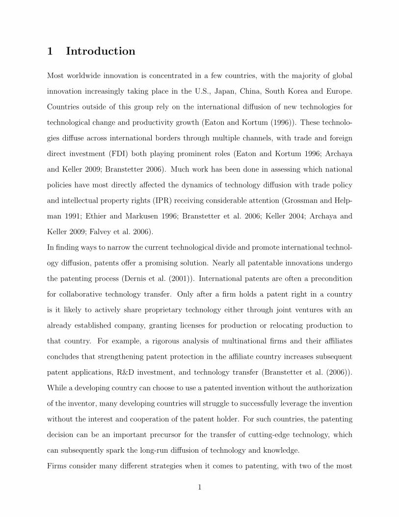
Abstract

How do firms decide where and when to patent? This paper develops a heteroge-

neous firm model of trade with endogenous rival entry where innovating firms compete

with rival firms on price. Patenting reduces the number of rival firms and provides

higher expected profits and increased markups from reduced competition and greater

appropriability. Countries with higher technology levels, more competition and better

patent protection have a higher proportion of entrants who patent. Industries follow a

U-shaped pattern of patenting depending on the variability of production and substi-

tutability. Using bilateral international patent flows, the model is calibrated to obtain

measures of country technology states and IP benefits. A look at the benefits of inter-

national patent treaties and its member countries highlights how nearly all countries

benefit from participating in patent treaties and that patent treaties have reduced ad-

ministrative fees for innovating firms by more than $7.2B in 2012. Further simulations

suggest that technology gains and trade liberalization between 1996 and 2012 both

contributed substantially to the rise of international patents.

Keywords: Patents, international trade, heterogeneous firms, endogenous markups,

intellectual property rights, imperfect competition, patent agreements

JEL Codes: F12, F23, K11, L11, L60, O34

∗Thank you for comments and feedback provided by Robert Feenstra, Travis Lybbert, Giovanni Peri,Katheryn Russ, Deborah Swenson, Emin Dinlersoz, Farid Toubal, Greg Wright, Andrew McCallum and An-son Soderbery. Any opinions and conclusions expressed herein are those of the author and do not necessarilyrepresent the views of the U.S. Census Bureau. The research in this paper does not use any confidential Cen-sus Bureau information. All remaining errors are mine. This paper was previously titled ”Firm LocationalPatenting Decisions.”†Contact: nikolas.j.zolas@census.gov

1 Introduction

Most worldwide innovation is concentrated in a few countries, with the majority of global

innovation increasingly taking place in the U.S., Japan, China, South Korea and Europe.

Countries outside of this group rely on the international diffusion of new technologies for

technological change and productivity growth (Eaton and Kortum (1996)). These technolo-

gies diffuse across international borders through multiple channels, with trade and foreign

direct investment (FDI) both playing prominent roles (Eaton and Kortum 1996; Archaya

and Keller 2009; Branstetter 2006). Much work has been done in assessing which national

policies have most directly affected the dynamics of technology diffusion with trade policy

and intellectual property rights (IPR) receiving considerable attention (Grossman and Help-

man 1991; Ethier and Markusen 1996; Branstetter et al. 2006; Keller 2004; Archaya and

Keller 2009; Falvey et al. 2006).

In finding ways to narrow the current technological divide and promote international technol-

ogy diffusion, patents offer a promising solution. Nearly all patentable innovations undergo

the patenting process (Dernis et al. (2001)). International patents are often a precondition

for collaborative technology transfer. Only after a firm holds a patent right in a country

is it likely to actively share proprietary technology either through joint ventures with an

already established company, granting licenses for production or relocating production to

that country. For example, a rigorous analysis of multinational firms and their affiliates

concludes that strengthening patent protection in the affiliate country increases subsequent

patent applications, R&D investment, and technology transfer (Branstetter et al. (2006)).

While a developing country can choose to use a patented invention without the authorization

of the inventor, many developing countries will struggle to successfully leverage the invention

without the interest and cooperation of the patent holder. For such countries, the patenting

decision can be an important precursor for the transfer of cutting-edge technology, which

can subsequently spark the long-run diffusion of technology and knowledge.

Firms consider many different strategies when it comes to patenting, with two of the most

1

important factors being cost and timing (Livne 2006; Schneiderman 2007). In a survey of

U.S. manufacturing firms, Cohen et al. (2000) find that firms patent mainly to prevent imi-

tation and counterfeiting, but also for reasons such as patent blocking, negotiating licensing

agreements with other firms, preventing lawsuits and bullying their competitors to exit the

market. More recent work by Graham and Sichelman (2008) find that start-ups patent for

many of the same reasons listed above, but also for reasons such as making the firm ap-

pear more attractive for investment or acquisition. The cost of patenting can pile up very

quickly, with filing fees, agent fees and translation fees bringing the total application cost to

more than $10,000 per country application (Source: WIPO) in addition to the considerable

legal fees appropriated each year to defend patents. In addition, there are also transaction

costs, interaction costs with licensing professionals and knowledge costs of exposing ideas to

potential imitators. On the other hand, the benefits of patenting give the firm additional

market power, prevent counterfeiting and allows them to charge higher markups and seek

higher profits over the life of the patent (Horstmann et al. 1985; Owen-Smith and Powell

2001).

While the firm has many incentives to patent, our understanding of the market conditions

that attract patents is still vague. Much of the focus in the literature is focused on the

impact of IPR, but other country and industry-specific conditions may also play an impor-

tant role. For instance, a recent paper by Bilir (2014) finds that product life-cycle is a key

determinant in multinational activity abroad, where firms with longer product life-cycles

are more sensitive to intellectual property rights. This paper looks at how competition,

production variability, substitutability and country technology-levels impact international

patenting strategies. The paper accomplishes this by introducing a patenting decision com-

ponent into a Ricardian heterogeneous firm model of trade (similar to Bernard et al. (2003))

with imperfect competition (similar to de Blas and Russ (2015)). In the model, innovating

firms compete internationally with domestic rival firms on price (Bertrand competition). The

number of rivals and their productivities depend on the innovating firm’s own productivity

2

so that more productive innovating firms face a greater number of more competitive rivals.

This creates more incentive to patent. The model manages to maintain the producer-level

facts regarding the behavior and composition of exporting firms and multi-nationals in the

’new’ new trade theory, while allowing for cross-country and cross-industry differences to

determine the flows of international patenting. These cross-country and cross-industry dif-

ferences play a key role in deciding spatial patenting outcomes.

International patenting has important implications for development and is the topic of much

debate regarding international technology transfer. The role of patent rights figured promi-

nently in the original negotiations of the Trade-Related Aspects of Intellectual Property

Rights Agreement (TRIPS) in the Uruguay Round of GATT in 1994. Throughout these

negotiations developing countries expressed concern that stronger IPR would only benefit

wealthy countries that had already developed strong innovation capacity. Developed coun-

tries therefore agreed to a provision to provide incentives for firms to transfer technology

to developing countries and enable them to build a viable technological base (Article 66.2).

Implicit in this provision is the hope that offering stronger patent protection to foreign in-

novators might speed up the process of technology transfer. Where firms choose to patent

is therefore central in this debate.

Since the passing of the TRIPS agreement, the number of non-resident patent application

filings has risen from 305,000 in 1994 to more than 800,000 in 2012 (Source: WIPO IP Stat),

with the share of non-resident filings rising from 32% of total filings to 40% by 2006. In

addition, the set of ”core” countries that countries choose to apply to has also changed over

this time period, with firms focusing less on Europe and countries outside of the periphery,

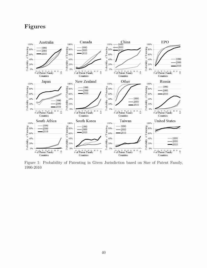
and shifting their attention towards Asia, and specifically China, Russia and Japan. Figure

1 plots the probability of patenting in the top 12 jurisdictions based on the size of the patent

family in 1990, 2000 and 2010. The United States remains firmly entrenched as the top

destination for international patents, followed by China, Japan and the European Patent

Office (EPO). The hierarchy of patent destinations has shifted dramatically, led by China’s

3

extraordinary rise as a key patenting destination.

[Figure 1 about here]

While trade-related factors are a key determinant of international patenting behavior,

these trends cannot only be explained by existing trade models. One of the key contributions

of this paper is to provide a specific framework to analyze the determinants of international

patenting. Using a database of patent families compiled by the World Intellectual Property

Organization (WIPO) and the EPO, the model backs out measures of country intellectual

property (IP) benefit, which considers both the degree of protection (probability that the

firm will receive monopolistic profits), reduction in competition and gain in markups for

firms. This measure of IP benefit differs from the traditional measures of IPR found in

Park (2008) since it considers additional factors such as the degree of competition within a

country and market size. Hence, small countries with limited competition who have strong

IPR measures, may have low measures of IP benefit.

The calibration of the model also provides annual measures for country technology states

and industry variability. The combination of parameters allows for comparisons of patent

flows based on these same parameters through policy experiments. The paper finds that

the net impact of global technology gains since 1996 led to a predicted gain of 38% more

patents in 2012. Similarly, the impact of a reduction in trade costs between 1996 and 2012

contributed to a nearly 43% increase in the number of global patents.

The contributions of this paper to the literature are several. The paper introduces a new

framework to analyze firm patenting and trade decisions, with endogenous rival entry and

endogenous markups. Empirically, this paper obtains measures of country IP benefit and

technology levels using existing international patent flows. This former measure considers

both the degree of protection, as well as the level of competition and market size by country.

This paper also measures the effectiveness of patent agreements on patent filings, finding

a significant increase in the number of patents exchanged worldwide and a reduction in

4

administrative costs resulting from these agreements. The next section defines the model and

outlines the process to calculate a numerical equilibrium. Section 3 describes the properties of

the equilibrium using simulations and parameter estimates. Section 4 describes the empirical

portion and constructs market-based measures of patent benefit. This is followed by the

conclusion.

2 Model

The core elements of the model are taken from a heterogeneous firm trade model, with

some key differences in the composition of rivals and ability of innovating firms to patent.

We start by describing the innovating firm whose productivity is drawn from a boundless

distribution. If/when the innovating firm competes in a market, the firm faces a number

of rivals whose distribution is bounded by the innovating firm’s productivity capabilities.

The innovating firm competes against the low-cost rival and the markup is determined by

Bertrand competition. The innovating firm can reduce the number of rivals the firm faces by

paying an additional fixed cost and patenting. No closed-form equilibrium solution is possible

and the model is solved analytically through numerical simulations, before parameterization.

2.1 Demand

Assume that that there are i = 1, ..., I countries where each country has the ability to produce

k = 1, ..., K different goods or industries. Next, assume only one factor of production, labor

Li, which is perfectly mobile across industries but not countries and paid wage wi. Each

good k is comprised of an infinite number of varieties, which will be indexed by ω ∈ Ω.

In each country, preferences are given by a representative consumer with a two-tier utility

function. The upper-tier utility function is Cobb-Douglas where the share of expenditure

on varieties from industry k in country i are given by αki where 0 ≤ αki ≤ 1. The lower-tier

utility function is CES with elasticity of substitution σk between varieties. Thus, in any

5

country i, the total expenditure on variety ω of good k will be given by:

xki (ω) =

(pki (ω)

P ki

)1−σk

αkiwiLi (1)

where P ki is the CES price index1. Given these assumptions, the consumer price index in

country i is given by Pi =∏K

k=1

(pki)αki .

2.2 Production and Innovation

Labor is the only factor used in production and is assumed to be perfectly mobile across types

and goods, but immobile across countries. Denote zki (ω) to be the measure of productivity of

variety ω in industry k. Next, assume that there are two types of firms in the world economy:

i.) Innovating firms who pay a one-time fixed cost of innovation Iki that allows them to draw

their productivity parameter z from an unbounded distribution and ii.) Imitating or rival

firms who do not pay an entry fee but are bounded in their productivity draws by the

innovating firms’ productive capability.

Both types of firms draw their productivity zki (ω) from the same distribution type. If we think

of innovating firms as repeatedly drawing ideas from a set of existing ideas, then the best (i.e.

most efficient) surviving idea takes on a Frechet (inverted Weibull) distribution F ki (z) with

positive support (see Eaton and Kortum (2009), Chapter 4). The Frechet distribution will

be governed by two separate parameters: a country specific technology parameter Ti which

will govern the mean of the distribution and an industry specific shape parameter θk > 1

that determines the heterogeneity of efficiency levels. The distribution for the innovating

firms is given by

F ki (z|Ti, θk) = Pr

[zki ≤ z

]= e−Tiz

−θk

(2)

1Given by P ki =(∑

ω′∈Ω pki (ω′)1−σk

)1/(1−σk)

6

A higher Ti implies higher technology and greater productivity on average, while a higher

θk means lower variability in labor efficiencies so that producers are more homogeneous.

In order to guarantee the existence of a well-defined CES price index P kj , assume that the

elasticity of substitution σki < 1 + θk.

Next, drop the superscript k and assume that the following holds for each industry type

k = 1, ..., K. Once the innovating firm in country i draws this parameter z, the firm decides

whether to pay a per-period fixed cost to enter the market and sell their good in market j,

f ∗ij. The innovating firm can choose to either export, paying a per-period fixed cost of fXij ,

along with iceberg trade costs dij and the home country wage of wi2. Or the firm can relocate

abroad, paying a higher per-period fixed cost fFij and the destination country’s wages as in

Helpman et al. (2004). For the purposes of this model, it makes no difference which method

the firm chooses to sell the good in destination j. The outcomes of the model will depend

only on the cost function after the firm makes this choice, which is denoted as cIij3.

Given CES demand, the optimal price for the innovating firm will be to charge a CES or

monopolistic markup. Without any rivals and with the exception of different productivity

distributions, the equilibrium and properties of the equilibrium are similar to the results

obtained in Helpman et al. (2004).

2.3 Production and Imitation

Assume that for each new variety ω in each market j, the innovating firm faces some number

rj of rivals or imitators who compete with the firm on price (Bertrand) as in Bernard et al.

2All trade costs are positive (dij ≥ 1)and I assume that trade barriers obey the triangle inequality sothat dij ≤ dindnj for all i, j and n.

3Formally, cIij is written as

cIij =

wjzIi

zIi ≥[

(σ)σ

(σ−1)σ−1

fFij−fXij

αjYj

(w1−σj − (widij)

1−σ)] 1

σ−1

Pj

widijzIi

Otherwise

Where Yj is country-level income (equal to wjLj). Assuming(wjwi

)σ−1

fFij > dσ−1ij fXij . The firm will make

the choice to either export or commit FDI using the CES/monopolistic markup.

7

(2003) and de Blas and Russ (2015). Unlike the previous models, however, the number of

rivals and possible imitators in each country is endogenously determined by the productivity

parameter of the innovating firm4 The rival firms’ marginal cost distributions will be bounded

by the marginal costs of the innovating firm, so they are never more efficient at producing

variety ω than the firm who invented it. Since the firms compete on price, this implies that

the rival firms will never make positive profits unless the innovating firm decides to exit.

However, each rival draws only one time and do not pay a fixed cost of entry or innovation

cost and are able to enter and exit at any given time, thereby behaving as a ’credible threat’

to the innovating firm.

Denote the rival productivity in country j as zRj . Each of the rivals have constant returns to

scale and their marginal costs are given by cRj (ω) =wj

zRj (ω). The rivals face the same demand

functions as their counterparts, so that the profit function is similar to the innovating firm’s

profit function, with the exception that each rival pays a per-period fixed cost fRj to enter into

the market. Due to this per-period fixed cost, there exists a non-zero cutoff cost parameter

cRj that governs whether the rival has the low-cost necessary to compete and serve as a

credible threat. This cutoff condition cRj is determined by assuming monopolistic pricing

and setting the profit equal to zero so that cRj corresponds to the productivity threshold

sufficient to cover the fixed per-period overhead costs.

cRj =

[(σ)σ

(σ − 1)σ−1

fRjαjYj

] 11−σ

Pj (3)

Rivals who draw a cost parameter c ≤ cRj are permanent entrants and remain as credible

threats in the market for as long as the innovating firm competes. Rivals who draw c > cRj

4As de Blas and Russ (2015) note, Bernard et al. (2003) assumes that the number of rivals for any givenproduct is a random variable determined by a Poisson distribution. This assumption allows the number ofrivals to cancel out in the analysis (see Eaton and Kortum (2009), Chapter 4) as the primary focus is on thelow-cost rival. On the other hand, de Blas and Russ (2015) assume that the number of rivals is determinedsolely by the free-entry condition, and is therefore unaffected by the productivity of the innovating firm.In this paper, the number of rivals is determined jointly by the zero-profit condition and innovating firm’sproductivity, providing a bound to both the number of rival firms and their productivities.

8

can never enter and are not deemed credible. Each rival draws their cost parameters c from

a similar shape distribution as the innovating firm (Wiebull), but their support is truncated

by the marginal costs of the innovating firm which will be denoted as cIij5. The CDF of the

rivals’ cost function in country j is6

GRj (c|cIij, Tj, θ) = 1− e−Tjw

−θj

(cθ−(cIij)

θ)

(4)

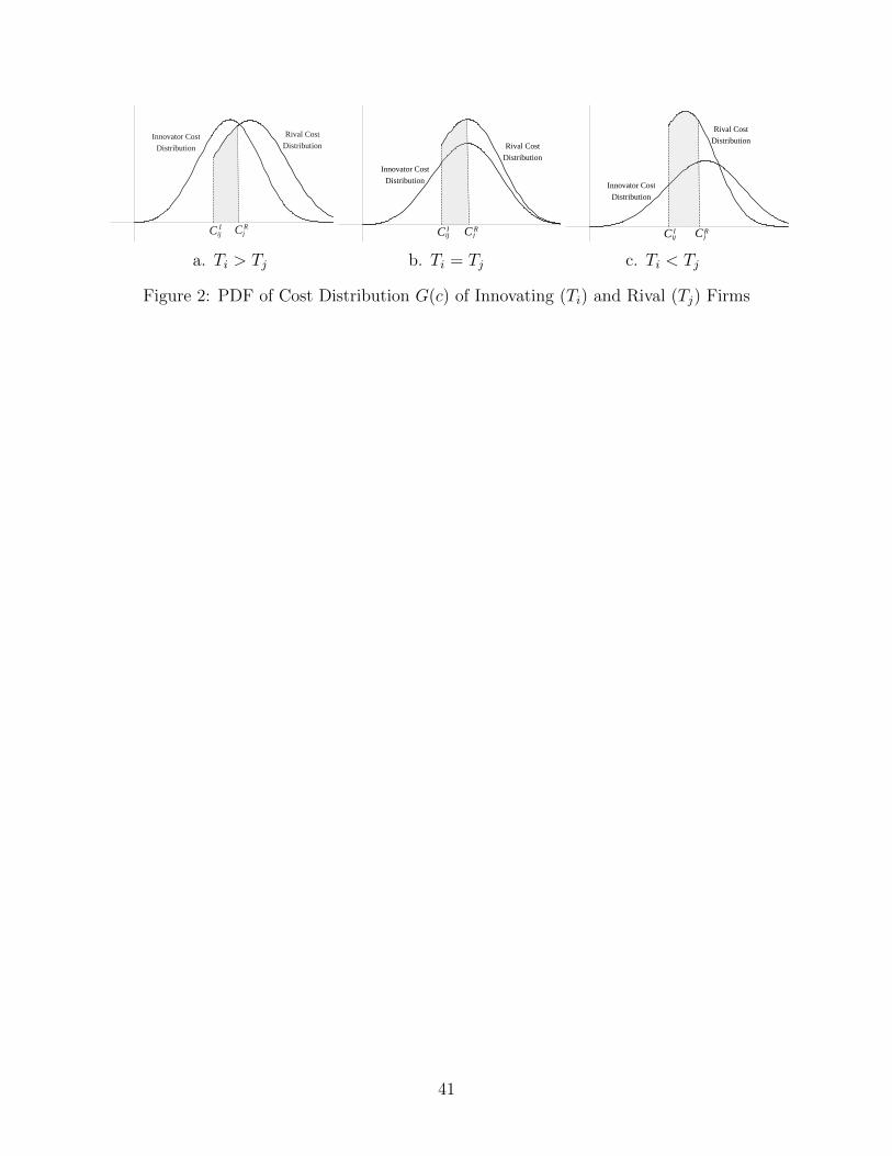
A depiction of the rival and innovating firms’ distributions is given below in Figure 2. In each

chart, the leftmost c represents the cost parameter for the innovating firm and shows a left-

truncation of the rivals’ cost distribution. The rightmost c is the equivalent cost parameter

for the cutoff condition for rival entry (given as the inverse of zRj , so that the area in between

the two lines is the ex-ante probability of successful entry by the rivals in country j. The

figure depicts three separate charts that are differentiated by the technology levels in the

destination country. Both the state of technology and variability in productivity in each

country-industry will determine the number of rivals and their productivities. In Figure 2a,

the technology for the innovating firm’s country is higher than the country of the rival firms.

Figure 2a shows that the innovating firm from country i will not only face relatively fewer

rivals, but also those rivals have lower average productivity than the innovating firm. In

Figure 2c, the opposite occurs where the country of the rival firms has higher technology

and the innovating firm not only faces more competition, but each competitor will have cost

parameters that are closer to the innovating firm’s cost parameter.

5Note that the definition of cIij will vary by innovating firm type (exporting or FDI).6Formula for a left-truncated Weibull distribution can be found on pages 134-135 in Rinne (2009). Note

that the corresponding productivity CDF for the rivals is given by

FRj(z|zIi , Tj , θ

)= e−Tj

(z−θ−

(wj

widij

)−θ(zIi )

−θ)

for exporting firms and

FRj(z|zIi , Tj , θ

)= e−Tj

(z−θ−(zIi )

−θ)

for FDI firms, where zIi is the productivity parameter of the innovating firm.

9

[Figure 2 about here]

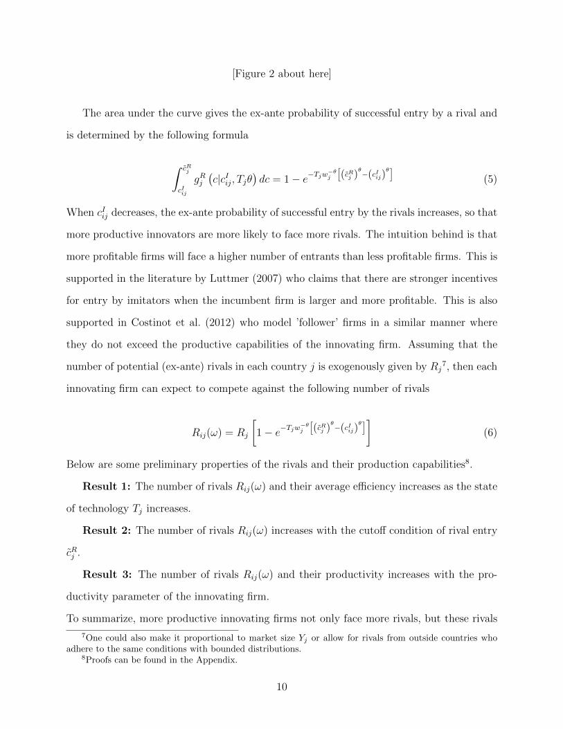
The area under the curve gives the ex-ante probability of successful entry by a rival and

is determined by the following formula

∫ cRj

cIij

gRj(c|cIij, Tjθ

)dc = 1− e−Tjw

−θj

[(cRj )

θ−(cIij)

θ]

(5)

When cIij decreases, the ex-ante probability of successful entry by the rivals increases, so that

more productive innovators are more likely to face more rivals. The intuition behind is that

more profitable firms will face a higher number of entrants than less profitable firms. This is

supported in the literature by Luttmer (2007) who claims that there are stronger incentives

for entry by imitators when the incumbent firm is larger and more profitable. This is also

supported in Costinot et al. (2012) who model ’follower’ firms in a similar manner where

they do not exceed the productive capabilities of the innovating firm. Assuming that the

number of potential (ex-ante) rivals in each country j is exogenously given by Rj7, then each

innovating firm can expect to compete against the following number of rivals

Rij(ω) = Rj

[1− e−Tjw

−θj

[(cRj )

θ−(cIij)

θ]]

(6)

Below are some preliminary properties of the rivals and their production capabilities8.

Result 1: The number of rivals Rij(ω) and their average efficiency increases as the state

of technology Tj increases.

Result 2: The number of rivals Rij(ω) increases with the cutoff condition of rival entry

cRj .

Result 3: The number of rivals Rij(ω) and their productivity increases with the pro-

ductivity parameter of the innovating firm.

To summarize, more productive innovating firms not only face more rivals, but these rivals

7One could also make it proportional to market size Yj or allow for rivals from outside countries whoadhere to the same conditions with bounded distributions.

8Proofs can be found in the Appendix.

10

are also more productive on average. Innovating firms can reduce the number of rivals they

face by increasing the cutoff condition for rival entry. Moving forward, consider the case

where cIij < cRj so that at least one rival exists at all times.

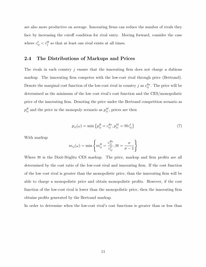
2.4 The Distributions of Markups and Prices

The rivals in each country j ensure that the innovating firm does not charge a dubious

markup. The innovating firm competes with the low-cost rival through price (Bertrand).

Denote the marginal cost function of the low-cost rival in country j as cR∗ij . The price will be

determined as the minimum of the low cost rival’s cost function and the CES/monopolistic

price of the innovating firm. Denoting the price under the Bertrand competition scenario as

pBij and the price in the monopoly scenario as pMij , prices are then

pij(ω) = minpBij = cR∗ij , p

Mij = mcIij

(7)

With markup

mij(ω) = min

mBij =

cR∗ijcIij

,m =σ

σ − 1

Where m is the Dixit-Stiglitz CES markup. The price, markup and firm profits are all

determined by the cost ratio of the low-cost rival and innovating firm. If the cost function

of the low cost rival is greater than the monopolistic price, than the innovating firm will be

able to charge a monopolistic price and obtain monopolistic profits. However, if the cost

function of the low-cost rival is lower than the monopolistic price, then the innovating firm

obtains profits generated by the Bertrand markup.

In order to determine when the low-cost rival’s cost functions is greater than or less than

11

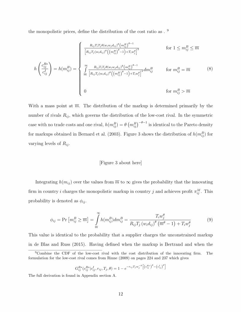
the monopolistic prices, define the distribution of the cost ratio as . 9

h

(cR∗ijcIij

)= h(mB

ij) =

RijTiTjθ(wiwjdij)θ(mBij)

θ−1[RijTj(widij)

θ((mBij)

θ−1)

+Tiwθj

]2 for 1 ≤ mBij ≤ m

∞∫m

RijTiTjθ(wiwjdij)θ(mBij)

θ−1[RijTj(widij)

θ((mBij)

θ−1)

+Tiwθj

]2dmBij for mB

ij = m

0 for mBij > m

(8)

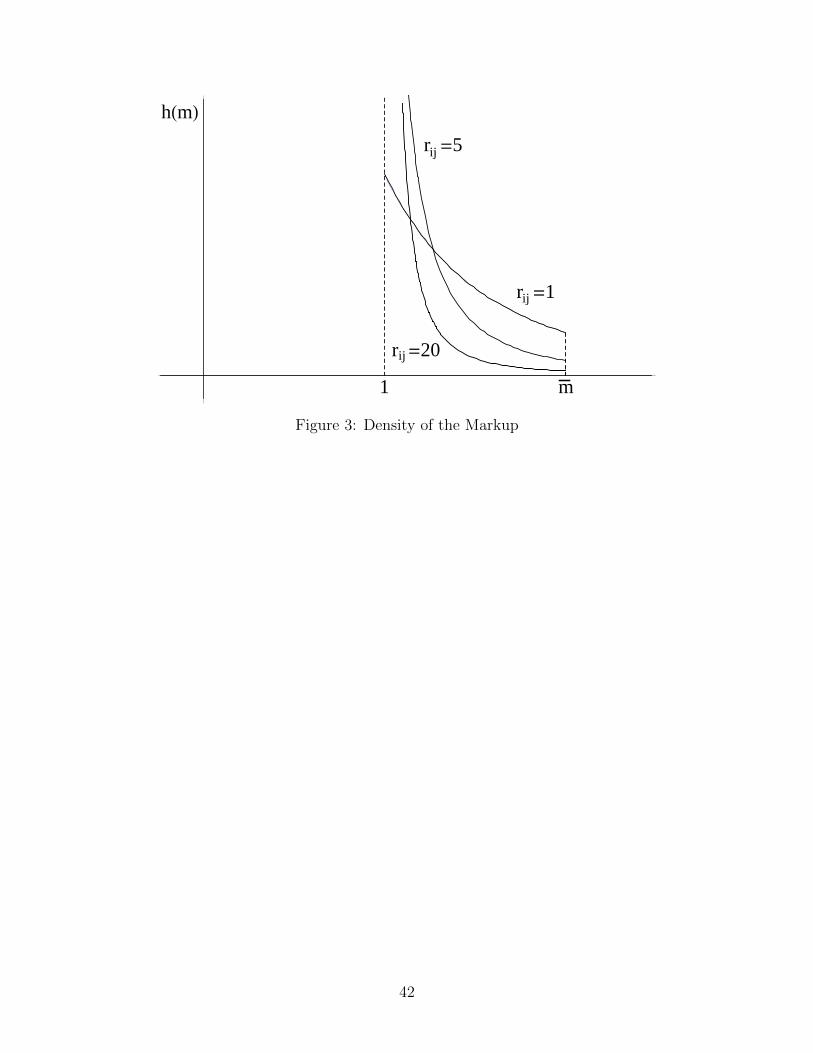
With a mass point at m. The distribution of the markup is determined primarily by the

number of rivals Rij, which governs the distribution of the low-cost rival. In the symmetric

case with no trade costs and one rival, h(mBij) = θ

(mBij

)−θ−1is identical to the Pareto density

for markups obtained in Bernard et al. (2003). Figure 3 shows the distribution of h(mBij) for

varying levels of Rij.

[Figure 3 about here]

Integrating h(mij) over the values from m to∞ gives the probability that the innovating

firm in country i charges the monopolistic markup in country j and achieves profit πMij . This

probability is denoted as φij.

φij = Pr[mBij ≥ m

]=

∞∫m

h(mBij)dm

Bij =

Tiwθj

RijTj (widij)θ (mθ − 1

)+ Tiwθj

(9)

This value is identical to the probability that a supplier charges the unconstrained markup

in de Blas and Russ (2015). Having defined when the markup is Bertrand and when the

9Combine the CDF of the low-cost rival with the cost distribution of the innovating firm. Theformulation for the low-cost rival comes from Rinne (2009) on pages 224 and 237 which gives

GR∗ij (cR∗ij |cIij , rij , Tj , θ) = 1− e−rijTjw−θj

[(cR∗ij )

θ−(cIij)θ]

The full derivation is found in Appendix section A.

12

markup will be CES, the innovating firm’s profit equation is

E[πIij(ω)

]= φijπ

Mij + (1− φij) E

[πBij]

(10)

=

(cIijPj

)1−σ

αjYj[φijV (m) + (1− φij)V

(mBij

)]− f ∗ij

where V (x) = x−σ(x − 1) and mBij = E

[mBij|mB

ij ≤ m]

is the expected value of the markup

when it is less than the CES markup10. This leads to the next set of results.

Result 4: The probability the innovating firm charges the CES markup in country j is

decreasing in contestability Rij11.

Result 5: The probability the innovating firm charges the CES markup in country j

increases as the cutoff condition for rival entry decreases and decreases as the innovating

firm becomes more productive (lower costs)12.

Result 6: The innovating firm’s expected profit E[πIij(ω)

]is decreasing in contestability

rij.

Result 7: The price of variety ω charged to consumers in country j is decreasing in

contestability Rij.

To sum up the results, the number of rivals negatively effects the innovating firm’s expected

profits, so that holding the innovating firm’s productivity constant, they will want to reduce

the number of rivals. Note that despite the increased contestability, innovating firms with

higher productivities still receive larger profits due to CRS and capturing a larger market

share. The next section looks at when the innovating firm decides to patent.

10The expected value of this is given by the formulam∫1

mijh(mij)1−H(m) dmij which has no closed-form solution.

11This result is similar to the findings in de Blas and Russ (2015) who similarly show that lower markupsoccur with increased contestability.

12It may seem counterintuitive that more productive firms are less likely to be monopolists, but note thatthe expected markup for the innovating firm increases with their productivity so that they still generatemore profits than low productivity firms.

13

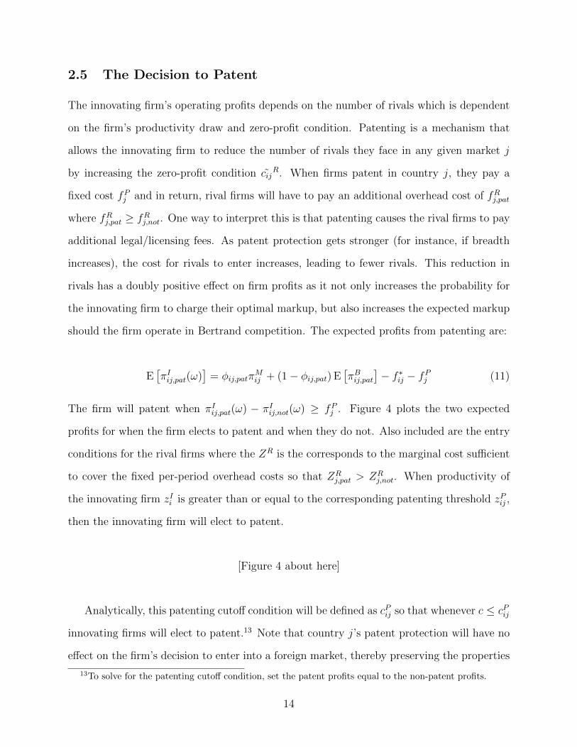
2.5 The Decision to Patent

The innovating firm’s operating profits depends on the number of rivals which is dependent

on the firm’s productivity draw and zero-profit condition. Patenting is a mechanism that

allows the innovating firm to reduce the number of rivals they face in any given market j

by increasing the zero-profit condition cijR. When firms patent in country j, they pay a

fixed cost fPj and in return, rival firms will have to pay an additional overhead cost of fRj,pat

where fRj,pat ≥ fRj,not. One way to interpret this is that patenting causes the rival firms to pay

additional legal/licensing fees. As patent protection gets stronger (for instance, if breadth

increases), the cost for rivals to enter increases, leading to fewer rivals. This reduction in

rivals has a doubly positive effect on firm profits as it not only increases the probability for

the innovating firm to charge their optimal markup, but also increases the expected markup

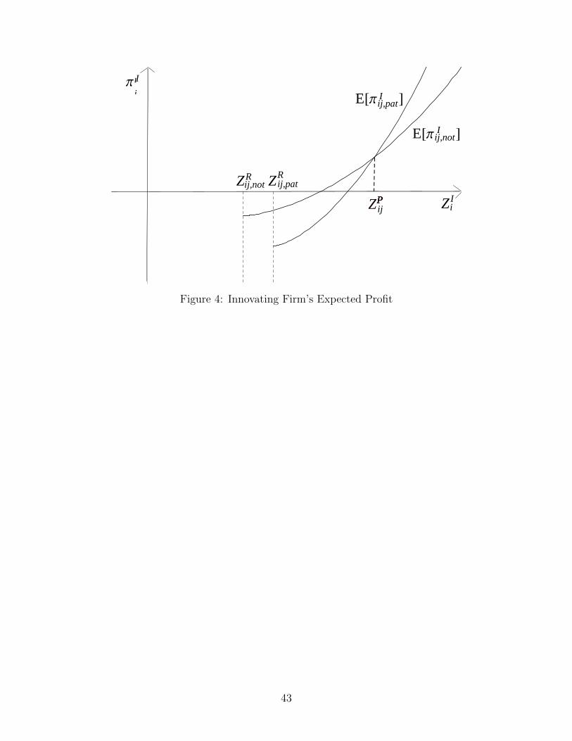
should the firm operate in Bertrand competition. The expected profits from patenting are:

E[πIij,pat(ω)

]= φij,patπ

Mij + (1− φij,pat) E

[πBij,pat

]− f ∗ij − fPj (11)

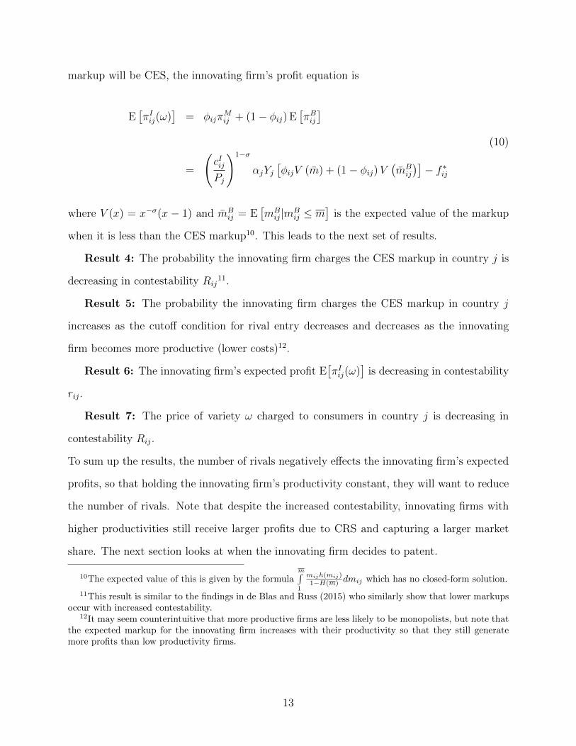
The firm will patent when πIij,pat(ω) − πIij,not(ω) ≥ fPj . Figure 4 plots the two expected

profits for when the firm elects to patent and when they do not. Also included are the entry

conditions for the rival firms where the ZR is the corresponds to the marginal cost sufficient

to cover the fixed per-period overhead costs so that ZRj,pat > ZR

j,not. When productivity of

the innovating firm zIi is greater than or equal to the corresponding patenting threshold zPij ,

then the innovating firm will elect to patent.

[Figure 4 about here]

Analytically, this patenting cutoff condition will be defined as cPij so that whenever c ≤ cPij

innovating firms will elect to patent.13 Note that country j’s patent protection will have no

effect on the firm’s decision to enter into a foreign market, thereby preserving the properties

13To solve for the patenting cutoff condition, set the patent profits equal to the non-patent profits.

14

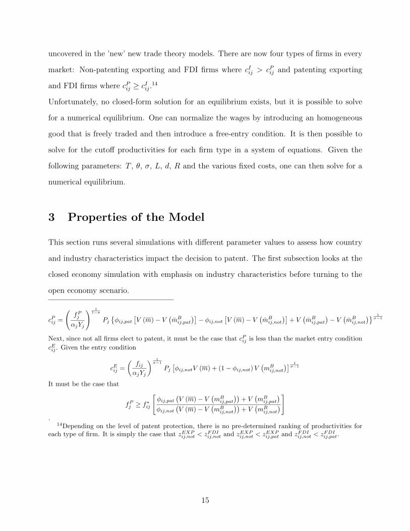
uncovered in the ’new’ new trade theory models. There are now four types of firms in every

market: Non-patenting exporting and FDI firms where cIij > cPij and patenting exporting

and FDI firms where cPij ≥ cIij.14

Unfortunately, no closed-form solution for an equilibrium exists, but it is possible to solve

for a numerical equilibrium. One can normalize the wages by introducing an homogeneous

good that is freely traded and then introduce a free-entry condition. It is then possible to

solve for the cutoff productivities for each firm type in a system of equations. Given the

following parameters: T , θ, σ, L, d, R and the various fixed costs, one can then solve for a

numerical equilibrium.

3 Properties of the Model

This section runs several simulations with different parameter values to assess how country

and industry characteristics impact the decision to patent. The first subsection looks at the

closed economy simulation with emphasis on industry characteristics before turning to the

open economy scenario.

cPij =

(fPjαjYj

) 11−σ

Pjφij,pat

[V (m)− V

(mBij,pat

)]− φij,not

[V (m)− V

(mBij,not

)]+ V

(mBij,pat

)− V

(mBij,not

) 1σ−1

Next, since not all firms elect to patent, it must be the case that cPij is less than the market entry condition

cEij . Given the entry condition

cEij =

(fijαjYj

) 1σ−1

Pj[φij,notV (m) + (1− φij,not)V

(mBij,not

)] 1σ−1

It must be the case that

fPj ≥ f∗ij

[φij,pat

(V (m)− V

(mBij,pat

))+ V

(mBij,pat

)φij,not

(V (m)− V

(mBij,not

))+ V

(mBij,not

)].

14Depending on the level of patent protection, there is no pre-determined ranking of productivities foreach type of firm. It is simply the case that zEXPij,not < zFDIij,not and zEXPij,not < zEXPij,pat and zFDIij,not < zFDIij,pat.

15

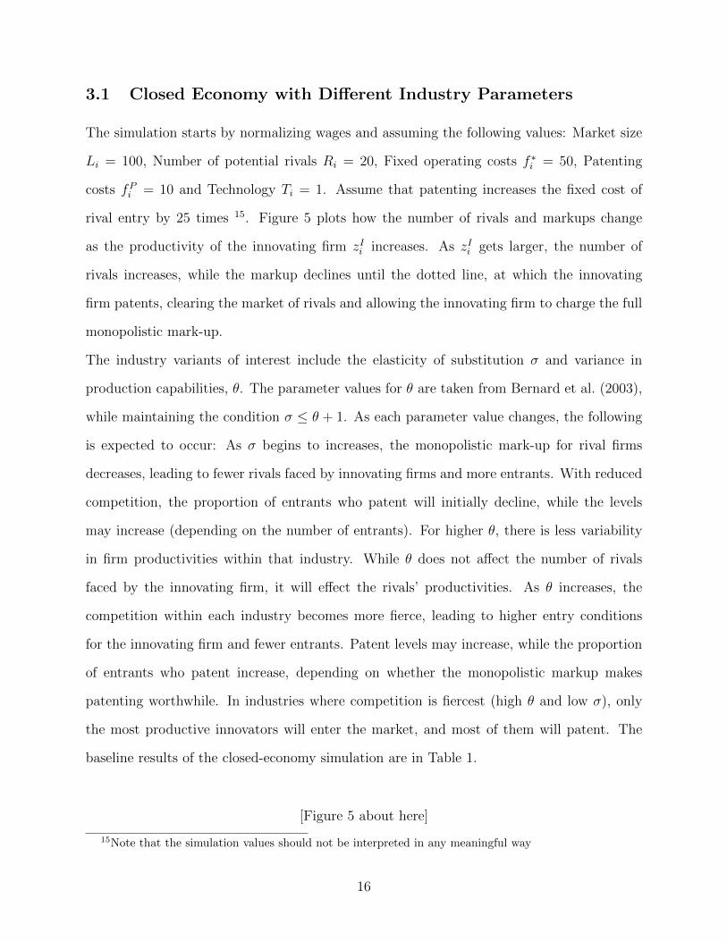
3.1 Closed Economy with Different Industry Parameters

The simulation starts by normalizing wages and assuming the following values: Market size

Li = 100, Number of potential rivals Ri = 20, Fixed operating costs f ∗i = 50, Patenting

costs fPi = 10 and Technology Ti = 1. Assume that patenting increases the fixed cost of

rival entry by 25 times 15. Figure 5 plots how the number of rivals and markups change

as the productivity of the innovating firm zIi increases. As zIi gets larger, the number of

rivals increases, while the markup declines until the dotted line, at which the innovating

firm patents, clearing the market of rivals and allowing the innovating firm to charge the full

monopolistic mark-up.

The industry variants of interest include the elasticity of substitution σ and variance in

production capabilities, θ. The parameter values for θ are taken from Bernard et al. (2003),

while maintaining the condition σ ≤ θ + 1. As each parameter value changes, the following

is expected to occur: As σ begins to increases, the monopolistic mark-up for rival firms

decreases, leading to fewer rivals faced by innovating firms and more entrants. With reduced

competition, the proportion of entrants who patent will initially decline, while the levels

may increase (depending on the number of entrants). For higher θ, there is less variability

in firm productivities within that industry. While θ does not affect the number of rivals

faced by the innovating firm, it will effect the rivals’ productivities. As θ increases, the

competition within each industry becomes more fierce, leading to higher entry conditions

for the innovating firm and fewer entrants. Patent levels may increase, while the proportion

of entrants who patent increase, depending on whether the monopolistic markup makes

patenting worthwhile. In industries where competition is fiercest (high θ and low σ), only

the most productive innovators will enter the market, and most of them will patent. The

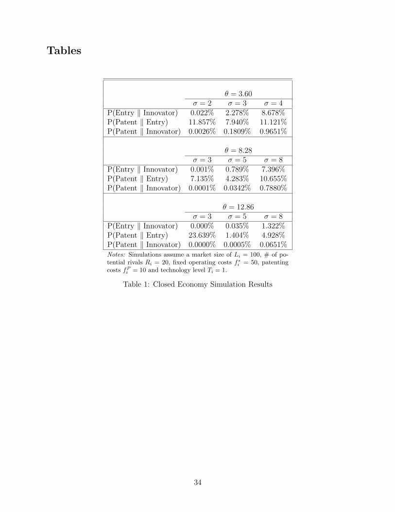
baseline results of the closed-economy simulation are in Table 1.

[Figure 5 about here]

15Note that the simulation values should not be interpreted in any meaningful way

16

[Table 1 about here]

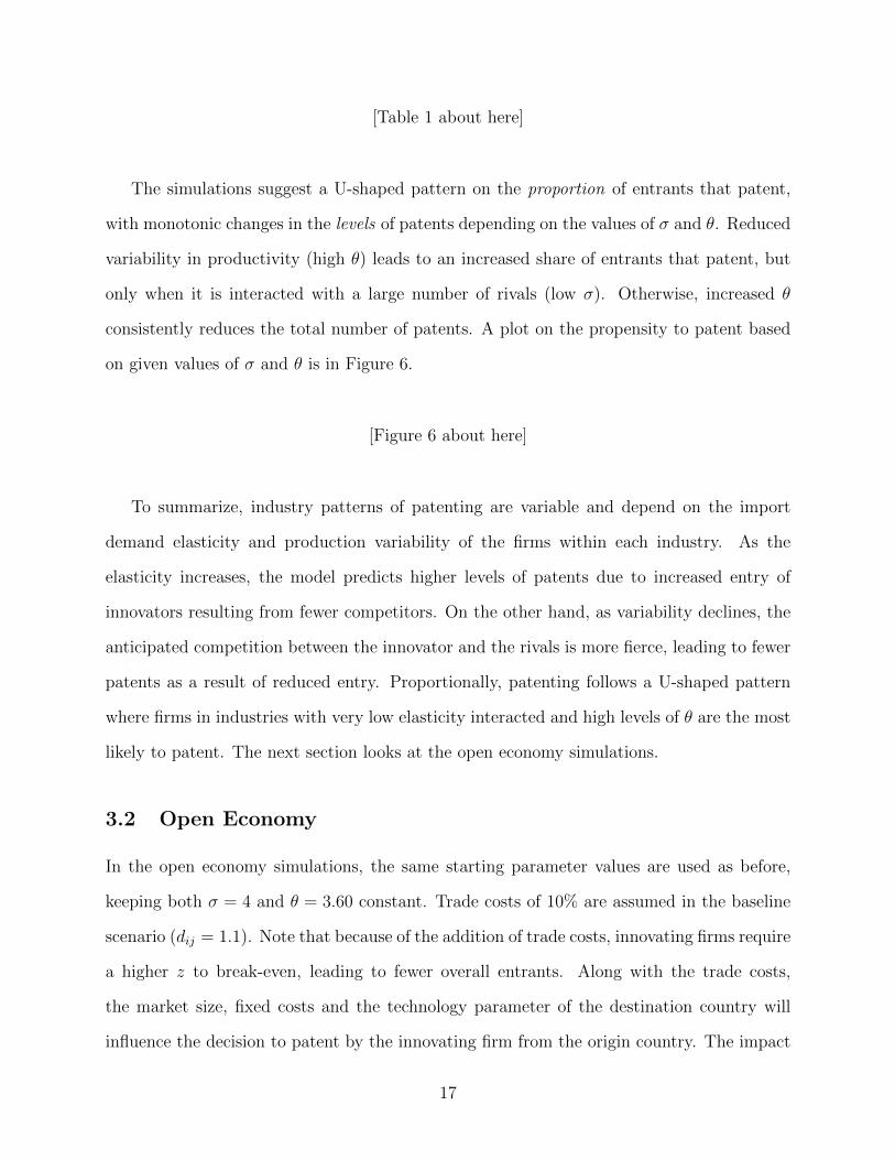
The simulations suggest a U-shaped pattern on the proportion of entrants that patent,

with monotonic changes in the levels of patents depending on the values of σ and θ. Reduced

variability in productivity (high θ) leads to an increased share of entrants that patent, but

only when it is interacted with a large number of rivals (low σ). Otherwise, increased θ

consistently reduces the total number of patents. A plot on the propensity to patent based

on given values of σ and θ is in Figure 6.

[Figure 6 about here]

To summarize, industry patterns of patenting are variable and depend on the import

demand elasticity and production variability of the firms within each industry. As the

elasticity increases, the model predicts higher levels of patents due to increased entry of

innovators resulting from fewer competitors. On the other hand, as variability declines, the

anticipated competition between the innovator and the rivals is more fierce, leading to fewer

patents as a result of reduced entry. Proportionally, patenting follows a U-shaped pattern

where firms in industries with very low elasticity interacted and high levels of θ are the most

likely to patent. The next section looks at the open economy simulations.

3.2 Open Economy

In the open economy simulations, the same starting parameter values are used as before,

keeping both σ = 4 and θ = 3.60 constant. Trade costs of 10% are assumed in the baseline

scenario (dij = 1.1). Note that because of the addition of trade costs, innovating firms require

a higher z to break-even, leading to fewer overall entrants. Along with the trade costs,

the market size, fixed costs and the technology parameter of the destination country will

influence the decision to patent by the innovating firm from the origin country. The impact

17

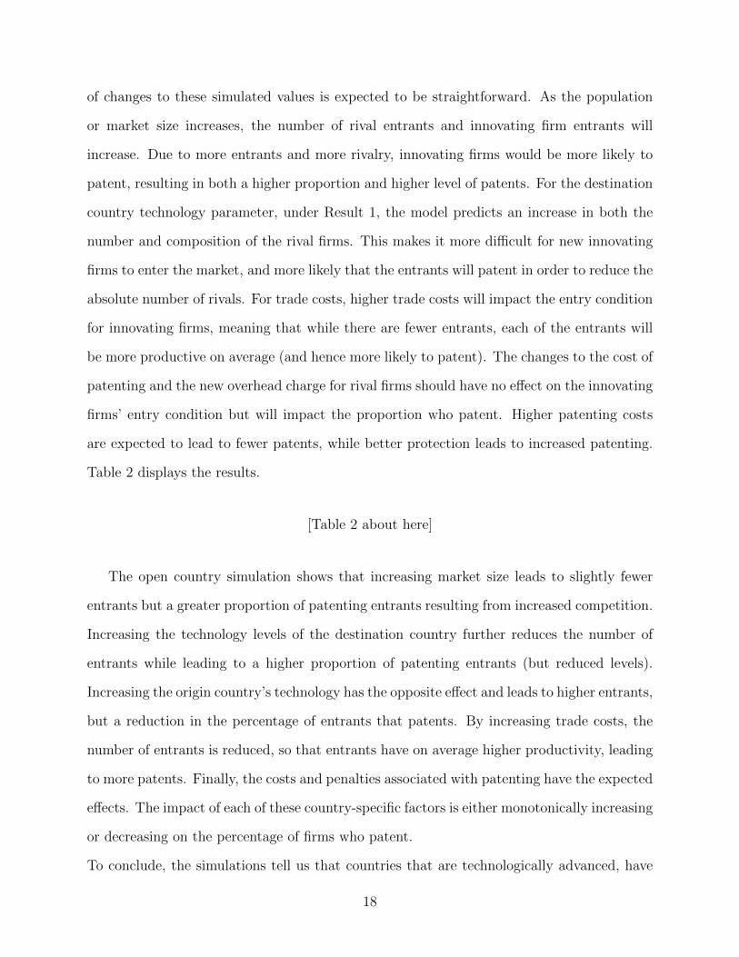
of changes to these simulated values is expected to be straightforward. As the population

or market size increases, the number of rival entrants and innovating firm entrants will

increase. Due to more entrants and more rivalry, innovating firms would be more likely to

patent, resulting in both a higher proportion and higher level of patents. For the destination

country technology parameter, under Result 1, the model predicts an increase in both the

number and composition of the rival firms. This makes it more difficult for new innovating

firms to enter the market, and more likely that the entrants will patent in order to reduce the

absolute number of rivals. For trade costs, higher trade costs will impact the entry condition

for innovating firms, meaning that while there are fewer entrants, each of the entrants will

be more productive on average (and hence more likely to patent). The changes to the cost of

patenting and the new overhead charge for rival firms should have no effect on the innovating

firms’ entry condition but will impact the proportion who patent. Higher patenting costs

are expected to lead to fewer patents, while better protection leads to increased patenting.

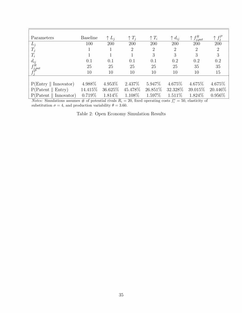
Table 2 displays the results.

[Table 2 about here]

The open country simulation shows that increasing market size leads to slightly fewer

entrants but a greater proportion of patenting entrants resulting from increased competition.

Increasing the technology levels of the destination country further reduces the number of

entrants while leading to a higher proportion of patenting entrants (but reduced levels).

Increasing the origin country’s technology has the opposite effect and leads to higher entrants,

but a reduction in the percentage of entrants that patents. By increasing trade costs, the

number of entrants is reduced, so that entrants have on average higher productivity, leading

to more patents. Finally, the costs and penalties associated with patenting have the expected

effects. The impact of each of these country-specific factors is either monotonically increasing

or decreasing on the percentage of firms who patent.

To conclude, the simulations tell us that countries that are technologically advanced, have

18

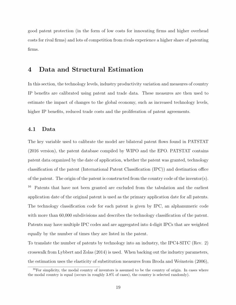
good patent protection (in the form of low costs for innovating firms and higher overhead

costs for rival firms) and lots of competition from rivals experience a higher share of patenting

firms.

4 Data and Structural Estimation

In this section, the technology levels, industry productivity variation and measures of country

IP benefits are calibrated using patent and trade data. These measures are then used to

estimate the impact of changes to the global economy, such as increased technology levels,

higher IP benefits, reduced trade costs and the proliferation of patent agreements.

4.1 Data

The key variable used to calibrate the model are bilateral patent flows found in PATSTAT

(2016 version), the patent database compiled by WIPO and the EPO. PATSTAT contains

patent data organized by the date of application, whether the patent was granted, technology

classification of the patent (International Patent Classification (IPC)) and destination office

of the patent. The origin of the patent is constructed from the country code of the inventor(s).

16 Patents that have not been granted are excluded from the tabulation and the earliest

application date of the original patent is used as the primary application date for all patents.

The technology classification code for each patent is given by IPC, an alphanumeric code

with more than 60,000 subdivisions and describes the technology classification of the patent.

Patents may have multiple IPC codes and are aggregated into 4-digit IPCs that are weighted

equally by the number of times they are listed in the patent.

To translate the number of patents by technology into an industry, the IPC4-SITC (Rev. 2)

crosswalk from Lybbert and Zolas (2014) is used. When backing out the industry parameters,

the estimation uses the elasticity of substitution measures from Broda and Weinstein (2006),

16For simplicity, the modal country of inventors is assumed to be the country of origin. In cases wherethe modal country is equal (occurs in roughly 3.8% of cases), the country is selected randomly).

19

which are also expressed in SITC Rev. 2.

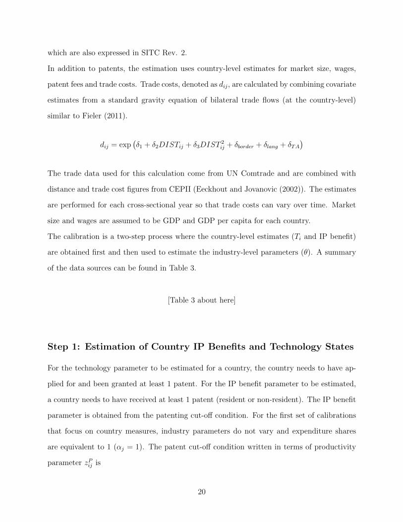
In addition to patents, the estimation uses country-level estimates for market size, wages,

patent fees and trade costs. Trade costs, denoted as dij, are calculated by combining covariate

estimates from a standard gravity equation of bilateral trade flows (at the country-level)

similar to Fieler (2011).

dij = exp(δ1 + δ2DISTij + δ3DIST

2ij + δborder + δlang + δTA

)The trade data used for this calculation come from UN Comtrade and are combined with

distance and trade cost figures from CEPII (Eeckhout and Jovanovic (2002)). The estimates

are performed for each cross-sectional year so that trade costs can vary over time. Market

size and wages are assumed to be GDP and GDP per capita for each country.

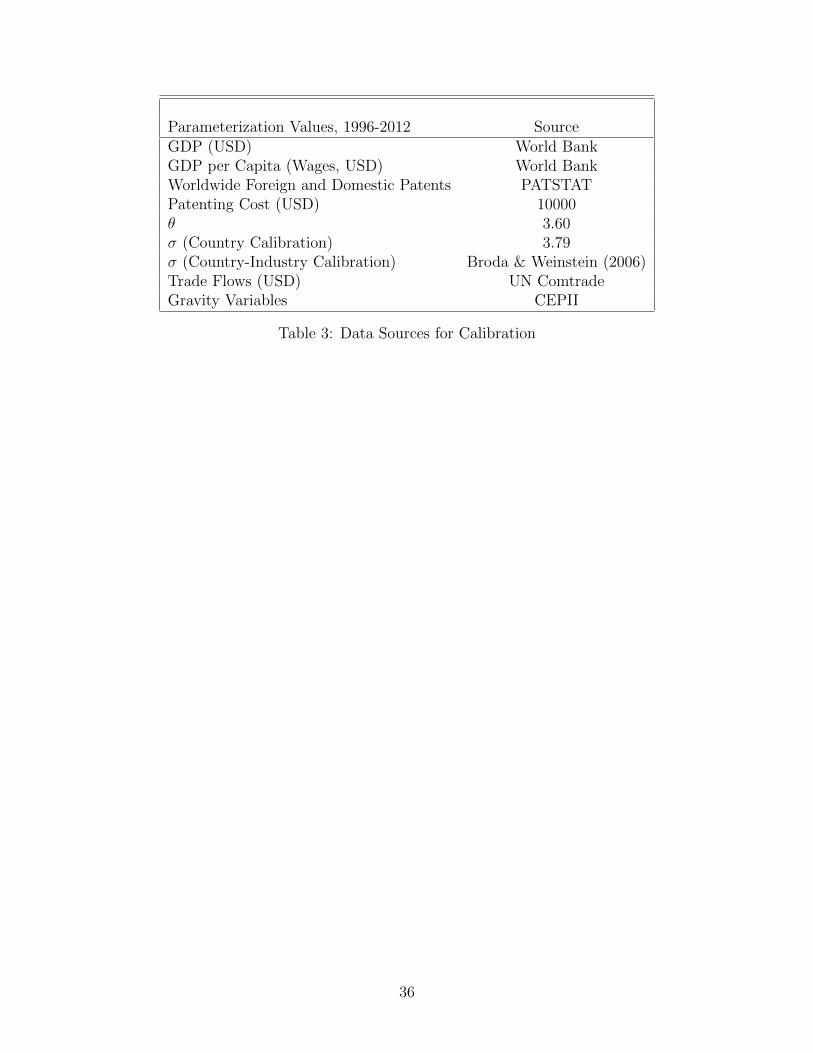
The calibration is a two-step process where the country-level estimates (Ti and IP benefit)

are obtained first and then used to estimate the industry-level parameters (θ). A summary

of the data sources can be found in Table 3.

[Table 3 about here]

Step 1: Estimation of Country IP Benefits and Technology States

For the technology parameter to be estimated for a country, the country needs to have ap-

plied for and been granted at least 1 patent. For the IP benefit parameter to be estimated,

a country needs to have received at least 1 patent (resident or non-resident). The IP benefit

parameter is obtained from the patenting cut-off condition. For the first set of calibrations

that focus on country measures, industry parameters do not vary and expenditure shares

are equivalent to 1 (αj = 1). The patent cut-off condition written in terms of productivity

parameter zPij is

20

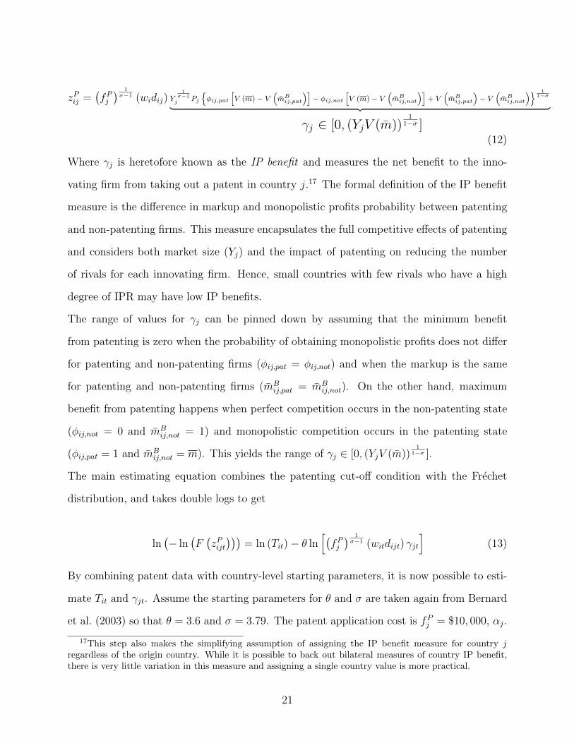
zPij =(fPj) 1σ−1 (widij) Y

1σ−1j Pj

φij,pat

[V (m)− V

(mBij,pat

)]− φij,not

[V (m)− V

(mBij,not

)]+ V

(mBij,pat

)− V

(mBij,not

) 11−σ︸ ︷︷ ︸

γj ∈ [0, (YjV (m))1

1−σ ](12)

Where γj is heretofore known as the IP benefit and measures the net benefit to the inno-

vating firm from taking out a patent in country j.17 The formal definition of the IP benefit

measure is the difference in markup and monopolistic profits probability between patenting

and non-patenting firms. This measure encapsulates the full competitive effects of patenting

and considers both market size (Yj) and the impact of patenting on reducing the number

of rivals for each innovating firm. Hence, small countries with few rivals who have a high

degree of IPR may have low IP benefits.

The range of values for γj can be pinned down by assuming that the minimum benefit

from patenting is zero when the probability of obtaining monopolistic profits does not differ

for patenting and non-patenting firms (φij,pat = φij,not) and when the markup is the same

for patenting and non-patenting firms (mBij,pat = mB

ij,not). On the other hand, maximum

benefit from patenting happens when perfect competition occurs in the non-patenting state

(φij,not = 0 and mBij,not = 1) and monopolistic competition occurs in the patenting state

(φij,pat = 1 and mBij,not = m). This yields the range of γj ∈ [0, (YjV (m))

11−σ ].

The main estimating equation combines the patenting cut-off condition with the Frechet

distribution, and takes double logs to get

ln(− ln

(F(zPijt)))

= ln (Tit)− θ ln[(fPj) 1σ−1 (witdijt) γjt

](13)

By combining patent data with country-level starting parameters, it is now possible to esti-

mate Tit and γjt. Assume the starting parameters for θ and σ are taken again from Bernard

et al. (2003) so that θ = 3.6 and σ = 3.79. The patent application cost is fPj = $10, 000, αj.

17This step also makes the simplifying assumption of assigning the IP benefit measure for country jregardless of the origin country. While it is possible to back out bilateral measures of country IP benefit,there is very little variation in this measure and assigning a single country value is more practical.

21

Trade costs dij are estimated using the technique used in Fieler (2011). The last remaining

variable definition is LHS variable F(zPijt), which is defined as the probability an innovating

firm from country i patents in country j at time t. This can be defined in a number of ways,

which will primarily impact the scalar parameter Tit18. For now, it is assumed to be the

number of bilateral patents divided by GDP (in $ million) for country i at time t. 19

Note that the initial estimating equation does not vary by industry and the industry-specific

variables, namely σ and θ have been aggregated and are unchanging. Each year t has I × J

observations to estimate I number of technology parameters and J number of IP benefit

parameters. These parameters are estimated using ordinary least squares. The values for

Tit and γjt are then used to calibrate the industry-level productivity variation θ.

Step 2: Estimation of Industry Productivity Variation

Once the estimates of technology Tit and IP benefit γjt are obtained, they are both used

to pin down the industry-variability measure θkt. To do this, the patent data is further

disaggregated to the origin-destination-SITC-year level. The same estimating equation (14)

is used, but σ is allowed to vary by industry. The values for the elasticity of substitution σ

are taken from Broda and Weinstein (2006). Expenditure shares for each country j (αjkt)

are assumed to be the share of total imports in product k to country j at time t

The terms of equation (13) are rearranged so that the bilateral patent percentage stays on

the LHS, but now the technology measures derived in the previous section are subtracted and

the observable variable on the RHS includes the destination country’s IP benefit measure

(along with the starting value assumptions for patent costs, sigma and trade costs). The

unknown variable, θ can then be measured for each k so that

18Because the scalar Tit has no real world basis, it is allowed to take on any value that is comparableacross countries over time.

19Alternative scalars have used R&D expenditures as a share of GDP and combination of R&D andpatents with very similar results

22

ln(− ln

(F(zPijkt

)))− ln

(Tit

)= θk ln

( fPjtαjkt

) 1σk−1

(witdijt) γjt

(14)

For each industry k, there are approximately I × J observations at time t. This parameter

is estimated using ordinary least squares. This completes the calibration. The next section

describes the results from the calibration and simulates changes to the some of the key

parameters.

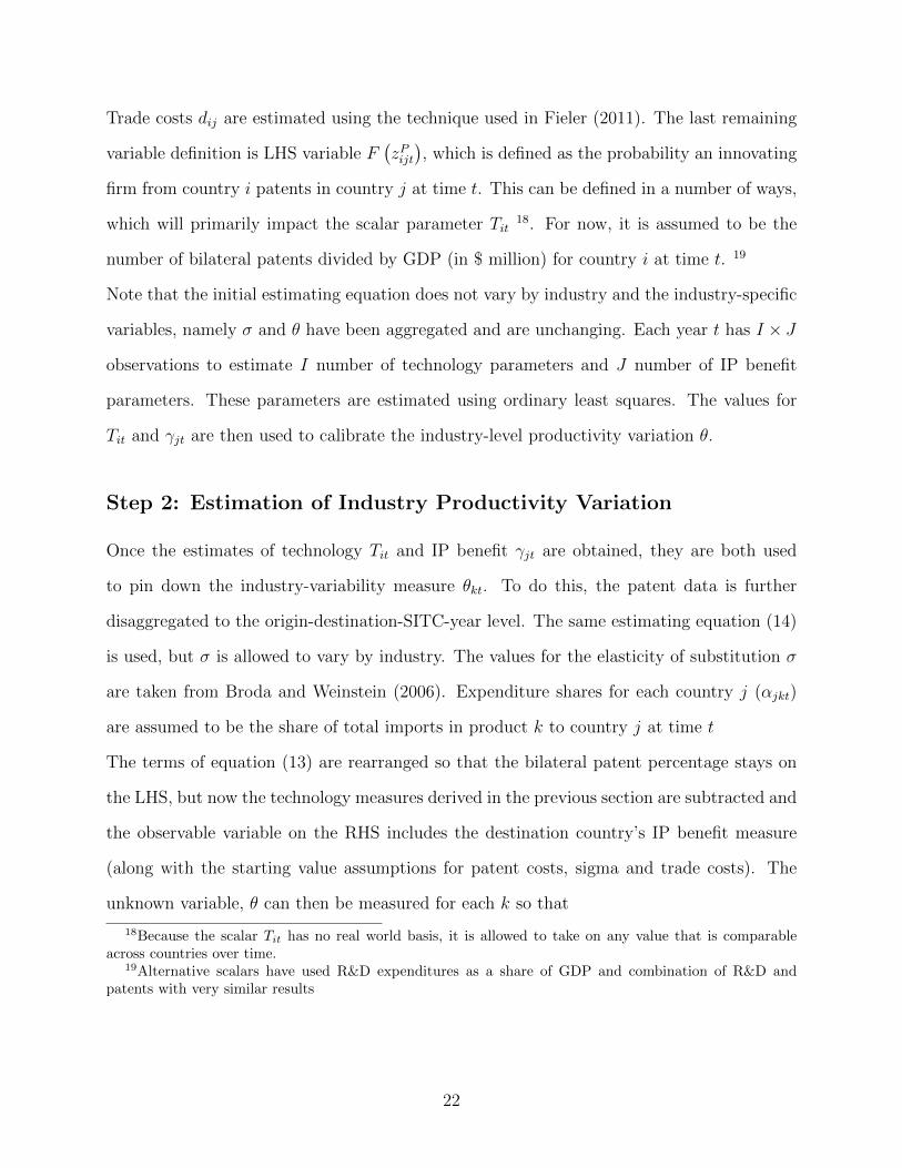
5 Results

The full parameter estimates for technology states, IP benefit and industry productivity

variability for each year, country and industry are available online. The estimated parameters

are used to predict bilateral patent flows and are compared with the actual flows in the data.

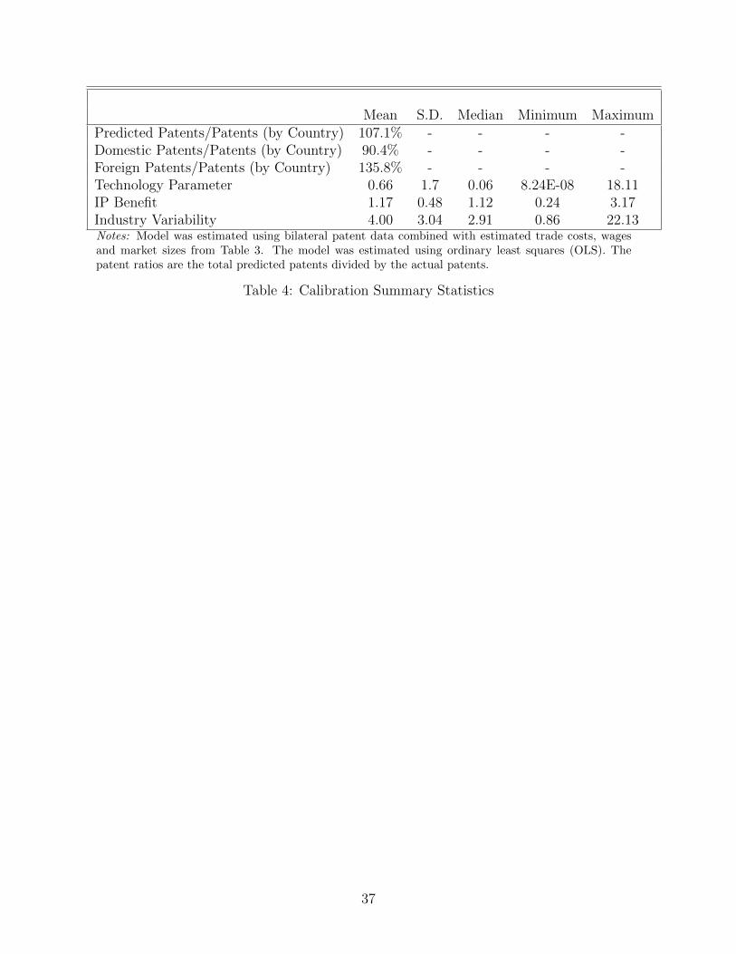
A summary of the results are provided in Table 4. The calibration is mostly successful. The

model is able to estimate total patent flows within 10% of actual patent flows by country

across all years. A plot of actual and predicted patent flows is provided in Figure 7. A

perfect fit would be clustered around the 45-degree line. The lowess smoothing line mostly

runs parallel to this, albeit shifted slightly to the right as the model tends to underestimate

domestic patents and overestimate foreign patent flows. Taken at face value, this might also

be suggestive that foreign patent flows should be higher than what is seen in the data. A

discussion of each of the parameters is given below.

[Table 4 about here]

[Figure 7 about here]

23

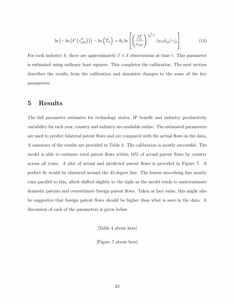
5.1 Technology States

Country technology levels take an extreme value form in Figure 8, with the majority of

countries possessing low technology levels. The technology parameter is driven primarily by

the number of originating patents and is consistent with the high concentration of patents

originating from relatively few countries. The technology levels are also consistent over time,

slowly rising in the late 1990s, declining somewhat in the early 2000s and then rising again

after 2006. The average growth rate between 1994 and 2012 across all countries with non-

zero patent flows in 2012 is 4.0% annually. Among the countries with the highest rates of

technology growth include China (18.2%), Turkey (10.4%) and the Czech Republic (9.3%),

while the countries with the slowest technology growth are South Africa (-22.5%), Algeria (-

16.6%) and Thailand (-1.6%). Unsurprisingly, country technology levels are highly correlated

with R&D expenditures as a share of GDP as found in Figure 9.

[Figure 8 about here]

[Figure 9 about here]

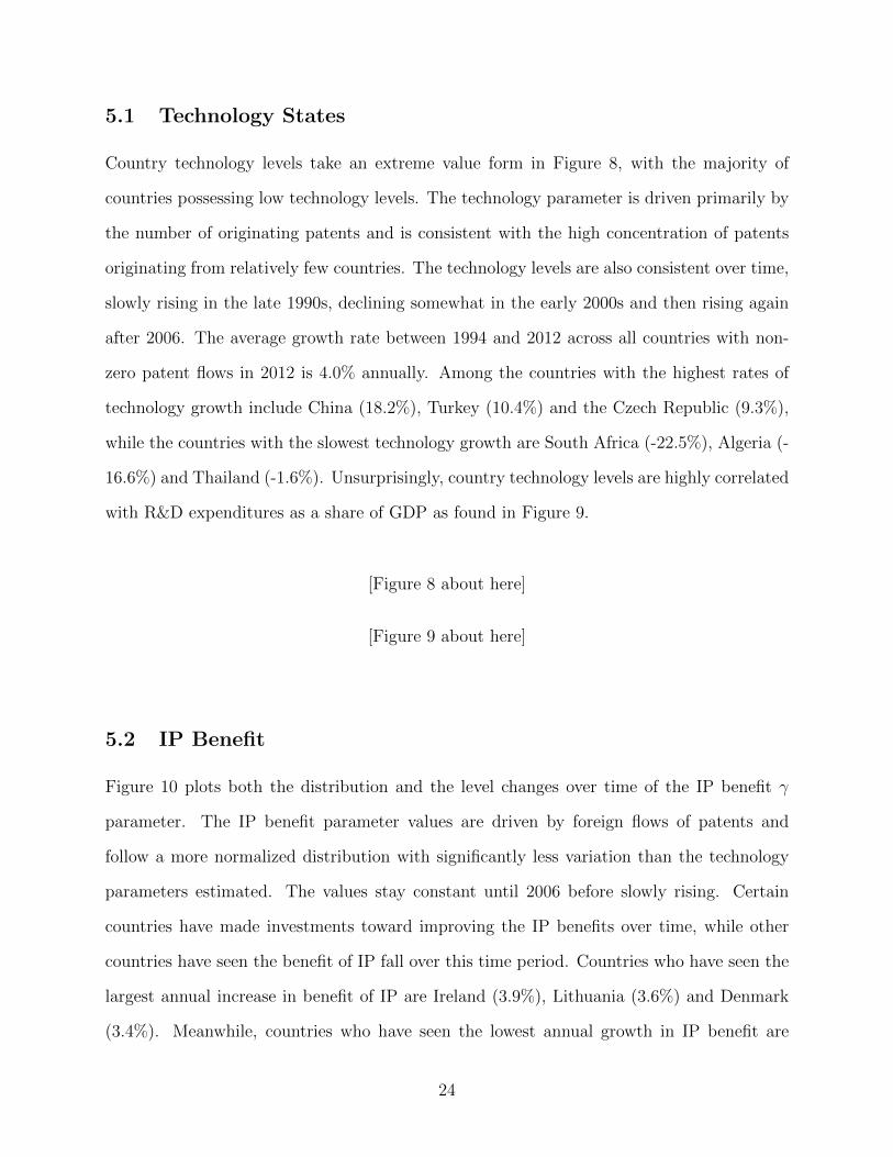
5.2 IP Benefit

Figure 10 plots both the distribution and the level changes over time of the IP benefit γ

parameter. The IP benefit parameter values are driven by foreign flows of patents and

follow a more normalized distribution with significantly less variation than the technology

parameters estimated. The values stay constant until 2006 before slowly rising. Certain

countries have made investments toward improving the IP benefits over time, while other

countries have seen the benefit of IP fall over this time period. Countries who have seen the

largest annual increase in benefit of IP are Ireland (3.9%), Lithuania (3.6%) and Denmark

(3.4%). Meanwhile, countries who have seen the lowest annual growth in IP benefit are

24

Azerbaijan (-4.8%), Singapore (-2.8%) and China (-0.9%). The inclusion of China as one of

the slower growing countries in terms of IP benefit may be surprising. However, despite the

growth of foreign patents to China over this time period, this growth appears to have not

kept pace with the economic growth.

[Figure 10 about here]

Despite the importance of market size in terms of calibrating IP benefits, IP protection

also figures prominently in the calculation. Figure 11 plots the IP benefit with traditional

measures of IPR, as found in Park (2008). While the IP benefit is positively correlated with

figures found in Park (2008), there are a number of notable differences. Namely, countries

who are also part of patent treaties tend to have lower IP benefits than might otherwise be

predicted. This is primarily due to firms electing to apply for a patent within the patent

treaty, as opposed to the individual country. Hence, the individual country benefit may not

be so high. When the patent treaty member countries are removed as the right hand side

shows, the relationship between IP benefit and IPR is more robust.

[Figure 11 about here]

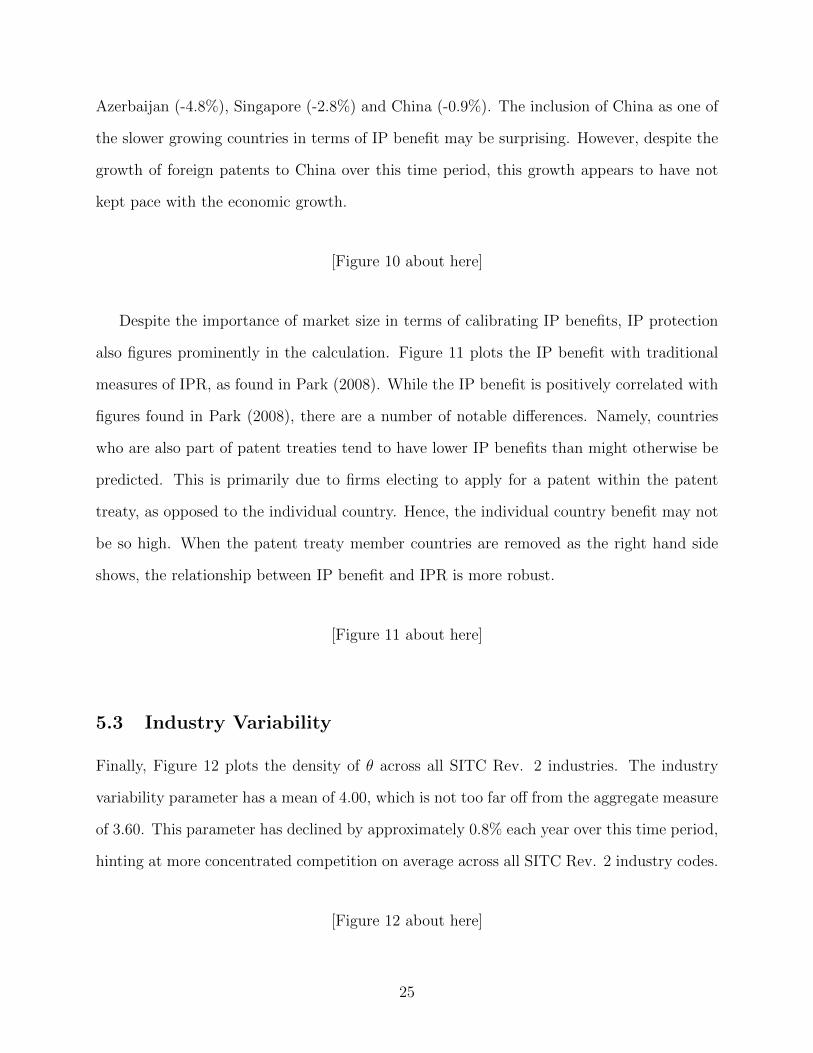
5.3 Industry Variability

Finally, Figure 12 plots the density of θ across all SITC Rev. 2 industries. The industry

variability parameter has a mean of 4.00, which is not too far off from the aggregate measure

of 3.60. This parameter has declined by approximately 0.8% each year over this time period,

hinting at more concentrated competition on average across all SITC Rev. 2 industry codes.

[Figure 12 about here]

25

5.4 Patent Agreements

As hinted in the previous section, the IP benefits for countries in patent treaties tend to

be lower than what one would predict given a country’s IPR and market size. One of the

benefits of the model is that it is possible to measure the IP benefit of existing patent treaties

and compare them with IP benefit of the countries that make up the patent treaty. A patent

treaty’s effectiveness can be determined by the number of patents that are applied through

the agreement versus the number of patents that are applied for in the individual countries

that make up each patent agreement. Across the entire sample, the average difference in IP

benefit between the patent treaty and the countries that make up the patent treaty is 0.41,

an almost 1 s.d. increase in the average country’s IP benefit.

There are 5 separated international patent treaties listed in the patent data. These include

the European Patent Organization (EPO), Eurasian Patent Organization (EAO), African

Regional Intellectual Property Organization (ARIPO), the African Intellectual Property Or-

ganization (AIPO) and Gulf Cooperation Council (GCC). Note that AIPO did not have

enough data points of the member countries to make a proper comparison. In nearly all

cases, one would expect that patent agreements lead to increased patenting resulting from

scale effects and lower administrative fees. In cases where the benefit of the individual

country would be higher, this may be due to enforcement issues within the agreement.

[Figure 13 about here]

Figure 13 compares the IP benefit of each of the patent agreements with the IP benefits

in each of the member countries. Member countries who receive no patents outside of the

patent treaty are not included in the plots. These countries are the largest beneficiaries of

the patent agreements as they would otherwise have had zero access to patents. The plots

show some interesting trends over time. In nearly all of the treaties, the benefit of belong-

ing to the treaty declines over the time period. Starting with the EPO treaty (which has

26

the highest IP benefit), all of the countries are better off from participating with member

countries of Great Britain (GB), Germany (DE) and France (FR) benefiting the least from

the agreement. Over time, the role of the EPO looks to be slowly diminishing as individual

country IP benefits increase and converge.

For countries in the Eurasian Patent Organization (EAO), roughly half of the countries have

higher individual benefits than the ones implied by the treaty, with Russia (RU) and Kaza-

khstan (KZ) never benefiting directly from the treaty. On the other hand, smaller countries

like Moldova (MD) and Azerbaijan (AZ) consistently benefit from being part of the EAO

treaty. For the African Regional Intellectual Property Organization (ARIPO) treaty, we find

the benefit split between the two member countries that also received patents as individual

countries (Kenya (KE) and the Sudan (SD)), with the differences in IP benefit being very

slight. There is also a benefit for all of the member countries in the Gulf Cooperation Council

(GCC).

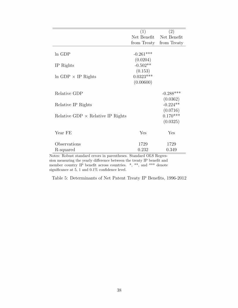
The differences in IP benefit across patent treaties are driven by two factors: levels of IPR

(both relative and absolute) and market size (both relative and absolute). Table 5 describes

a regression looking at how the net benefit of a patent treaty is impacted by the interaction

of these two factors. The results support the idea that member countries who have larger

market size or higher measures of IP rights tend to benefit less from patent treaties. On

the other hand, there does appear to be a positive effect for countries having both a large

market size and high IP rights. This may perhaps be indicative that patent treaties ben-

efit disproportionately more from having large countries with substantial IP protection as

member countries.

[Table 5 about here]

These results are the first empirical study that looks at the benefits of patent treaties.

While it would seem to be obvious that patenting through a treaty would be advantageous

for the innovating firm since it reduces the fixed costs of patenting, many firms still opt to

27

patent through the individual country only. This may be due to a variety of factors relating

to the patent treaty, such as differences in enforcement, stricter/looser guidelines, greater

exposure of ideas, redundancy, additional transaction costs over applying to a single country

or other reasons. The next section looks at the changes to worldwide patent flows resulting

from existing policy measures enacted over the time period.

5.5 Policy Experiments

The last empirical exercise looks at how changes to the parameter values impact the flow of

domestic and international patents. The comparison will look at the predicted patent flows

in 2012 resulting from the following policy experiments: i.) Having no patent treaties in

place (but countries have similar IP benefits as patent agreements), ii.) All countries having

the maximum technology state in 2012, iii.) All countries having the minimum technology

state in 2012, iv.) Constant technology states (1996 levels), v.) Cost of patenting declines

by 50%, vi.) Cost of patenting increases by 100%, vii.) Trade costs decline by 25% from

2012 levels, viii.) Trade costs increase by 25% from 2012 levels, ix.) Constant trade costs

(1996 levels). The first policy exercise (i.) will provide a dollar value measure of the benefits

of patent treaties for firms.

Table 6 estimates the cumulative worldwide patent flow resulting from each of these exper-

iments. Based on the starting values, Table 6 shows that without patent agreements (but

keeping the IP benefits of the patent agreement in place for member countries), foreign patent

flows would increase by more than 90%. A back-of-the-envelope calculation can measure the

economic benefits of patent agreements by comparing the differences in administrative fees

that patenting firms would face if no patent agreements were in place. For EPO member

countries, they received approximately 77,000 actual patents in 2012 according to PATSTAT

data. If the EPO was not in place, firms applying for a patent in all of the member countries

of the EPO where the IP benefit was high enough to justify the expenditure would have to

submit and apply for approximately 802,000 patents across all of the countries, a difference

28

of 725,000 patents. If the average application cost of these patents is $10,000, then firms ex-

perience a cost savings of approximately $7.25B in administrative fees from the EPO patent

agreement just in 2012.20 This is quite substantial and highlights the cost benefit of patent

treaties for innovating firms.

[Table 6 about here]

The other policy experiments tend to move in the direction predicted by the model and

the table can give a sense of how innovation levels would increase/decrease from changes to

technology levels, patent costs and trade costs. According to the model, if technology states

had remained at 1996 levels, innovation in 2012 (as measured by domestic patents) would

be 38% lower than the levels predicted. For patent costs, a reduction in the administrative

fees of 50% would lead to a 41% increase in patent output, while a doubling of patent costs

would lead to a reduction of around 24%.

Finally, trade costs also figure prominently in reducing or increasing patent flows. A 25%

reduction in trade costs are predicted to increase foreign patent flows by 44%. If trade costs

were to increase by 25%, corresponding foreign patent flows would decline by 28%. Finally,

if trade costs had remained the same as in 1996 in 2012, then foreign patent flows would

have declined by more than 75%.

To quickly summarize the empirical findings from the calibration exercise, nearly all countries

benefit from being a part of a patent treaty, with smaller markets benefiting more than

larger markets. The EPO patent treaty by itself, reduced patenting administrative costs

by approximately $7.25B in 2012. Policy experiments highlighted the role of technology

investments in increasing innovation rates, as well as how reducing administrative fees and

liberalizing trade can promote technology transfer. Had countries kept their 1996 technology

levels, patenting would be 38% lower than the levels predicted in 2012.

20This does not include the additional cost savings from having to continuously monitor and protect thesepatents

29

6 Conclusion

The goal of this paper is to better understand the conditions for multinational firms in decid-

ing where to seek international patent protection. These decisions are shown to have critical

implications for future investment, technology diffusion and economic growth, especially for

developing countries who linger outside of the patent core. This paper proposes a new type

of patenting decision model that borrows elements from the Ricardian heterogeneous firm

trade literature and can explain significant portions of spatial patenting patterns. The model

explains why countries with higher levels of technology, better patent protection and more

competition are able to solicit a greater number of patents. Using a generalized version of

the patenting cutoff condition, the model was able to calibrate patent benefit measures for

more than 80 countries of various size and income between 1994 and 2012. These patent

benefit measures take into account the actual patent flows to each country and differ with

alternative IPR indices by accounting for competition. In addition, the calibrated results

can also demonstrate how countries benefit from participating in patent treaties, with the

average country experiencing a nearly 1 s.d. improvement.

Although the model is described in full detail, several properties of the model remain un-

known. One of the more interesting aspects that has yet to be explored are the welfare ef-

fects that arise from strengthening IPRs and increasing technology transfer through patents.

While increased patenting activity would lead to higher expected profits of innovating firms

and greater diffusion, it is not clear what the negative effects are for consumers who may

gain new varieties, but must now pay higher markups. It may be the case that the gain in

welfare from the availability of new varieties outweighs the welfare loss from higher prices,

which is the argument put forth by developed countries in the TRIPS agreement. Analyzing

this question will help in addressing whether Article 66.2 of the TRIPS agreement has had a

positive or negative impact on developing countries who were forced to make improvements

to their IPRs.

Other possible extensions to the model include allowing foreign entry of rivals and incorpo-

30

rating an innovation component. Under the current framework, all of the potential rivals are

local. Given the assumptions on the productivity constraints of rivals, it makes little sense

to include foreign rivals since they would have to pay for the additional trade costs, making

it unlikely that they would ever become the low-cost rival. On the other hand, by making

the number of potential rivals in each country proportional to market size, it leaves open

the possibility of foreign entry. Including foreign rivals would add robustness to the model

since in many cases, multinational firms use patents as a deterrence and blocking device

for outside competitors trying to gain access to a particular market. Second, although the

model includes innovating firms, there is no decision variable for innovation. It is certainly

possible to include this component, since the profits for innovating firms are well-defined and

it would be interesting to see how rivals, patent protection and country variables interact in

influencing this decision.

Modeling international patent flows is an important step in understanding the process of

technology diffusion and the transfer of knowledge abroad. Many developing countries have

improved upon their intellectual property protection and this has shown to be increasingly ef-

fective, but it is not clear whether firms will continue to respond positively to these changes.

There also appears to be a trade-off between intellectual property rights and developing

industrial capacity (Falvey et al. (2006)). Nevertheless, the model provides a testable frame-

work for international patenting decisions and may lead to better policy in developing more

effective patent regimes.

31

References

Archaya, R. and W. Keller (2009, November). Technology transfer through imports. Cana-dian Journal of Economics 42 (4), 1411–1448.

Bernard, A., J. Eaton, J. B. Jensen, and S. Kortum (2003). Plants and productivity ininternational trade. American Economic Review 93 (4), 1268–1290.

Bilir, L. K. (2014). Patent laws, product life-cycle lengths, and multinational activity. Amer-ican Economic Review 104 (7), 1979–2013.

Branstetter, L. (2006, March). Is foreign direct investment a channel of knowledge spillovers?evidence from japan’s fdi in the united states. Journal of International Economics 68 (2),325–344.

Branstetter, L., R. Fisman, and C. F. Foley (2006, February). Do stronger intellectualproperty rights increase international technology transfer? empirical evidence from u.s.firm-level panel data. Quarterly Journal of Economics 121 (1), 321–349.

Broda, C. and D. Weinstein (2006, May). Globalization and the gains from variety. QuarterlyJournal of Economics 121 (2), 541–585.

Cohen, W., R. Nelson, and J. Walsh (2000, February). Protecting their intellectual assets:Appropriability conditions and why u.s. manufacturing firms patent (or not). NBERWorking Paper No. w7552 .

Costinot, A., D. Donaldson, and I. Komunjer (2012). What goods do countries trade? aquantitative explortaion of ricardo’s ideas. Review of Economic Studies 79 (2), 581–608.

de Blas, B. and K. Russ (2015). Understanding markups in the open economy. AmericanEconomic Journal: Macroeconomics 7 (2), 157–80.

Dernis, H., D. Guellec, and B. V. P. de la Potterie (2001). Using patent counts for cross-country comparisons of technology output. STI Review No. 27, OECD .

Eaton, J. and S. Kortum (1996, May). Trade in ideas: Patenting and productivity in theoecd. Journal of International Economics 40 (3-4), 251–278.

Eaton, J. and S. Kortum (2009). Technology in the global economy: A framework forquantitative analysis. Manuscript, University of Minnesota.

Eeckhout, J. and B. Jovanovic (2002, December). Knowledge spillovers and inequality.American Economic Review 92 (5), 1290–1307.

Ethier, W. and J. Markusen (1996, August). Multinational firms, technology diffusion andtrade. Journal of International Economics 41 (1-2), 1–28.

Falvey, R., N. Foster, and D. Greenaway (2006, November). Intellectual property rights andeconomic growth. Review of Development Economics 10 (4), 700–719.

Fieler, A. C. (2011). Nonhomotheticity and bilateral trade: Evidence and a quantitativeexplanation. Econometrica 79 (4), 1069–1101.

Graham, S. J. and T. Sichelman (2008, June). Why do start-ups patent. Berkeley TechnologyLaw Journal 23 (3), 1063–1098.

Grossman, G. and E. Helpman (1991). Innovation and Growth in the Global Economy.Cambridge, Mass.: MIT Press.

Helpman, E., M. Melitz, and S. Yeaple (2004, March). Export versus fdi with heterogeneousfirms. American Economic Review 94 (1), 300–316.

Horstmann, I., G. MacDonald, and A. Slivinski (1985, October). Patents as informationtransfer mechanisms: To patent or (maybe) not to patent. Journal of Political Econ-

32

omy 93 (5), 837–858.Keller, W. (2004, September). International technology diffusion. Journal of Economic

Literature 42 (3), 752–782.Livne, O. (2006, June). A cost conscious approach to patent application filings. Les Nou-

velles 41 (2), 115–119.Luttmer, E. (2007). Selection, growth, and the size distribution of firms. Quarterly Journal

of Economics 122 (3), 1103–1144.Lybbert, T. and N. Zolas (2014). Getting patents and economic data to speak to each

other: An ’algorithmic links with probabilities’ approach for joint analyses of patentingand economic activity. Research Policy 43 (3), 530–542.

Nadarajah, S. (2010). Distribution properties and estimation of the ratio of independentweibull random variables. Asta-advances in Statistical Analysis 94 (2), 231–246.

Owen-Smith, J. and W. Powell (2001). To patent or not: Faculty decisions and institutionalsuccess at technology transfer. Journal of Technology Transfer 26 (1-2), 99–114.

Park, W. (2008, May). International patent protection: 1960-2005. Research Policy 37 (4),761–766.

Prudnikov, A., Y. Brychkov, and O. Marichev (1986). Integrals and Series, Vols. 1, 2 and3. Amsterdam: Gordon and Breach Science Publishers.

Rinne, H. (2009). The Weibull Distribution: A Handbook. New York: Chapman & Hall/CRC.Schneiderman, A. (2007). Filing international patent applications under the patent coopera-

tion treaty (pct): Strategies for delaying costs and maximizing the value of your intellectualproperty worldwide. In A. Krattiger, R. Mahoney, and L. Nelson (Eds.), Intellectual Prop-erty Management In Health and Agricultural Innovation: A Handbook of Best Practices,pp. 941–952. MIHR: Oxford, U.K. and PIPRA: Davis, U.S.A.

33

Tables

θ = 3.60σ = 2 σ = 3 σ = 4

P(Entry ‖ Innovator) 0.022% 2.278% 8.678%P(Patent ‖ Entry) 11.857% 7.940% 11.121%P(Patent ‖ Innovator) 0.0026% 0.1809% 0.9651%

θ = 8.28σ = 3 σ = 5 σ = 8

P(Entry ‖ Innovator) 0.001% 0.789% 7.396%P(Patent ‖ Entry) 7.135% 4.283% 10.655%P(Patent ‖ Innovator) 0.0001% 0.0342% 0.7880%

θ = 12.86σ = 3 σ = 5 σ = 8

P(Entry ‖ Innovator) 0.000% 0.035% 1.322%P(Patent ‖ Entry) 23.639% 1.404% 4.928%P(Patent ‖ Innovator) 0.0000% 0.0005% 0.0651%Notes: Simulations assume a market size of Li = 100, # of po-tential rivals Ri = 20, fixed operating costs f∗i = 50, patentingcosts fPi = 10 and technology level Ti = 1.

Table 1: Closed Economy Simulation Results

34

Parameters Baseline ↑ Lj ↑ Tj ↑ Ti ↑ dij ↑ fRj,pat ↑ fPjLj 100 200 200 200 200 200 200Tj 1 1 2 2 2 2 2Ti 1 1 1 3 3 3 3dij 0.1 0.1 0.1 0.1 0.2 0.2 0.2fRj,pat 25 25 25 25 25 35 35fPj 10 10 10 10 10 10 15

P(Entry ‖ Innovator) 4.988% 4.953% 2.437% 5.947% 4.675% 4.675% 4.675%P(Patent ‖ Entry) 14.415% 36.625% 45.478% 26.851% 32.328% 39.015% 20.446%P(Patent ‖ Innovator) 0.719% 1.814% 1.108% 1.597% 1.511% 1.824% 0.956%Notes: Simulations assumes # of potential rivals Ri = 20, fixed operating costs f∗i = 50, elasticity ofsubstitution σ = 4, and production variability θ = 3.60.

Table 2: Open Economy Simulation Results

35

Parameterization Values, 1996-2012 SourceGDP (USD) World BankGDP per Capita (Wages, USD) World BankWorldwide Foreign and Domestic Patents PATSTATPatenting Cost (USD) 10000θ 3.60σ (Country Calibration) 3.79σ (Country-Industry Calibration) Broda & Weinstein (2006)Trade Flows (USD) UN ComtradeGravity Variables CEPII

Table 3: Data Sources for Calibration

36

Mean S.D. Median Minimum MaximumPredicted Patents/Patents (by Country) 107.1% - - - -Domestic Patents/Patents (by Country) 90.4% - - - -Foreign Patents/Patents (by Country) 135.8% - - - -Technology Parameter 0.66 1.7 0.06 8.24E-08 18.11IP Benefit 1.17 0.48 1.12 0.24 3.17Industry Variability 4.00 3.04 2.91 0.86 22.13Notes: Model was estimated using bilateral patent data combined with estimated trade costs, wagesand market sizes from Table 3. The model was estimated using ordinary least squares (OLS). Thepatent ratios are the total predicted patents divided by the actual patents.

Table 4: Calibration Summary Statistics

37

(1) (2)Net Benefit Net Benefitfrom Treaty from Treaty

ln GDP -0.261***(0.0204)

IP Rights -0.502**(0.153)

ln GDP × IP Rights 0.0323***(0.00600)

Relative GDP -0.288***(0.0362)

Relative IP Rights -0.224**(0.0716)

Relative GDP × Relative IP Rights 0.170***(0.0325)

Year FE Yes Yes

Observations 1729 1729R-squared 0.232 0.349

Notes: Robust standard errors in parentheses. Standard OLS Regres-sion measuring the yearly difference between the treaty IP benefit andmember country IP benefit across countries. *, **, and *** denotesignificance at 5, 1 and 0.1% confidence level.

Table 5: Determinants of Net Patent Treaty IP Benefits, 1996-2012

38

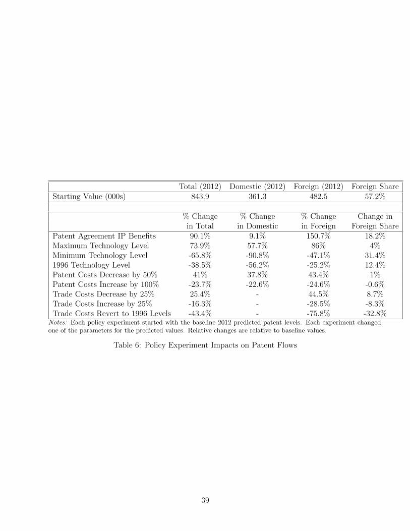
Total (2012) Domestic (2012) Foreign (2012) Foreign ShareStarting Value (000s) 843.9 361.3 482.5 57.2%

% Change % Change % Change Change inin Total in Domestic in Foreign Foreign Share

Patent Agreement IP Benefits 90.1% 9.1% 150.7% 18.2%Maximum Technology Level 73.9% 57.7% 86% 4%Minimum Technology Level -65.8% -90.8% -47.1% 31.4%1996 Technology Level -38.5% -56.2% -25.2% 12.4%Patent Costs Decrease by 50% 41% 37.8% 43.4% 1%Patent Costs Increase by 100% -23.7% -22.6% -24.6% -0.6%Trade Costs Decrease by 25% 25.4% - 44.5% 8.7%Trade Costs Increase by 25% -16.3% - -28.5% -8.3%Trade Costs Revert to 1996 Levels -43.4% - -75.8% -32.8%

Notes: Each policy experiment started with the baseline 2012 predicted patent levels. Each experiment changedone of the parameters for the predicted values. Relative changes are relative to baseline values.

Table 6: Policy Experiment Impacts on Patent Flows

39

Figures

Figure 1: Probability of Patenting in Given Jurisdiction based on Size of Patent Family,1990-2010

40

Innovator Cost

Distribution

Rival Cost

Distribution

C CI Rij j C C

Innovator Cost

Distribution

Rival Cost

Distribution

I Rij j

Rival Cost

Distribution

Innovator Cost

Distribution

C CI Rij j

a. Ti > Tj b. Ti = Tj c. Ti < Tj

Figure 2: PDF of Cost Distribution G(c) of Innovating (Ti) and Rival (Tj) Firms

41

m

hHmL

1

r =5

r =1

ij

ij

r =20ij

Figure 3: Density of the Markup

42

ZRij,not ZR

ij,pat

ZP

E@Π D

E@Π D

ij,pat

ij,not

PPij Zi

Πi

j

I

I

I

I

Figure 4: Innovating Firm’s Expected Profit

43

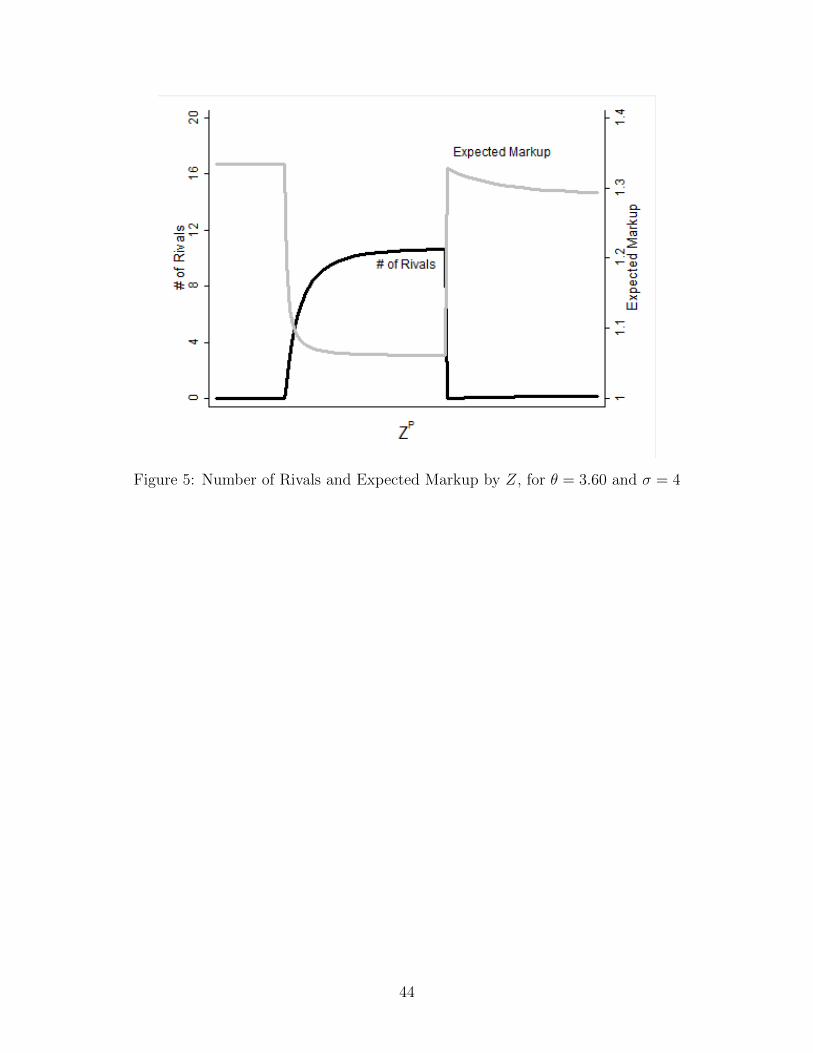
Figure 5: Number of Rivals and Expected Markup by Z, for θ = 3.60 and σ = 4

44

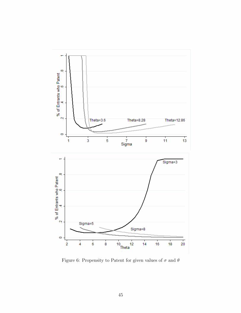
Figure 6: Propensity to Patent for given values of σ and θ

45

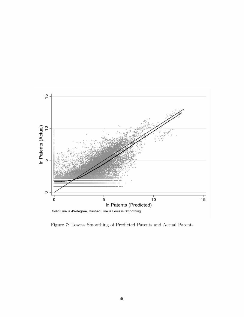
Figure 7: Lowess Smoothing of Predicted Patents and Actual Patents

46

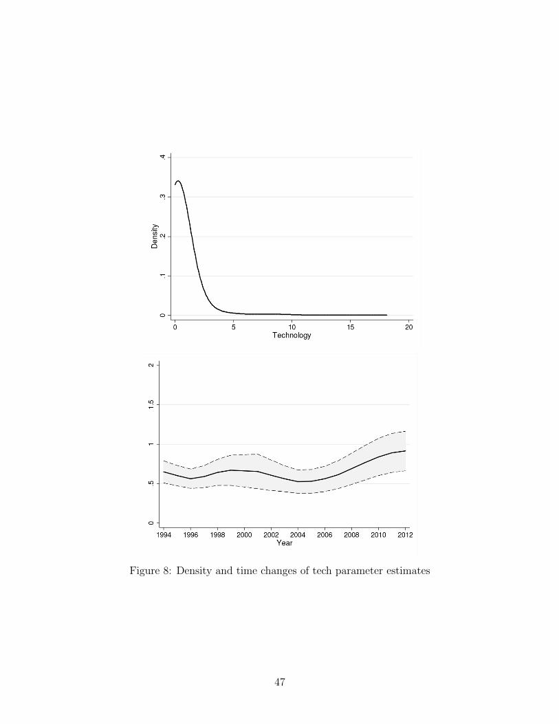
Figure 8: Density and time changes of tech parameter estimates

47

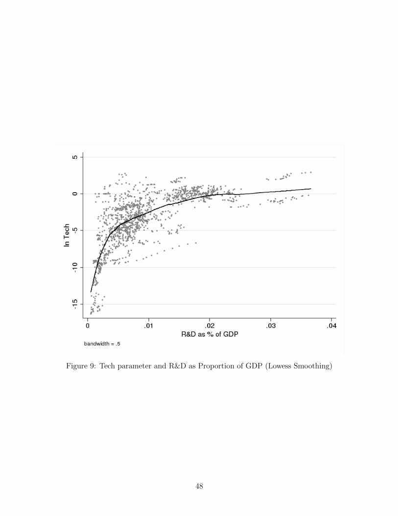
Figure 9: Tech parameter and R&D as Proportion of GDP (Lowess Smoothing)

48

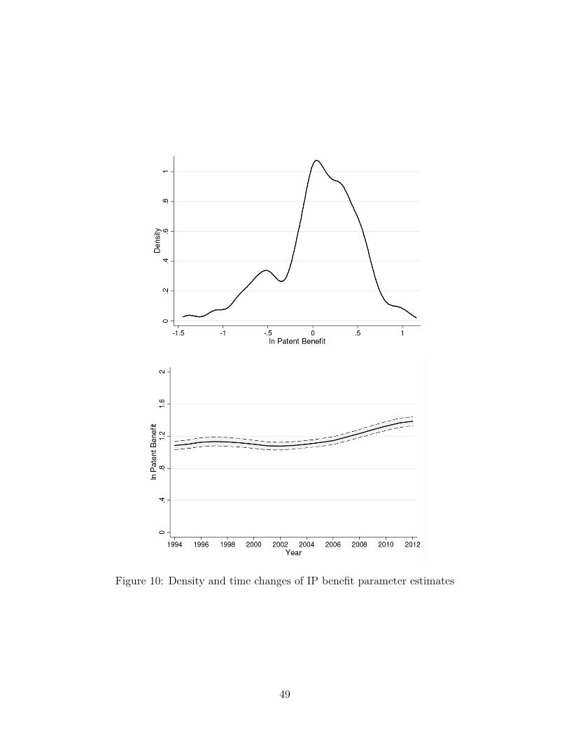
Figure 10: Density and time changes of IP benefit parameter estimates

49

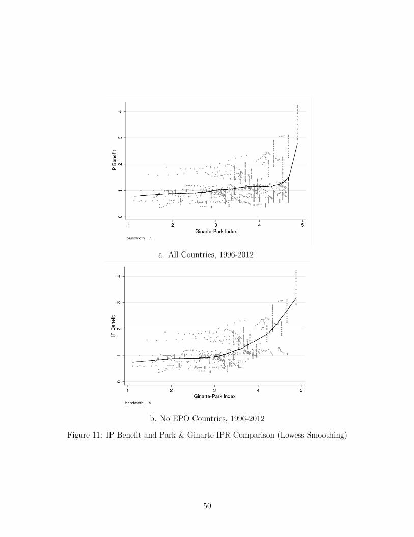
a. All Countries, 1996-2012

b. No EPO Countries, 1996-2012

Figure 11: IP Benefit and Park & Ginarte IPR Comparison (Lowess Smoothing)

50

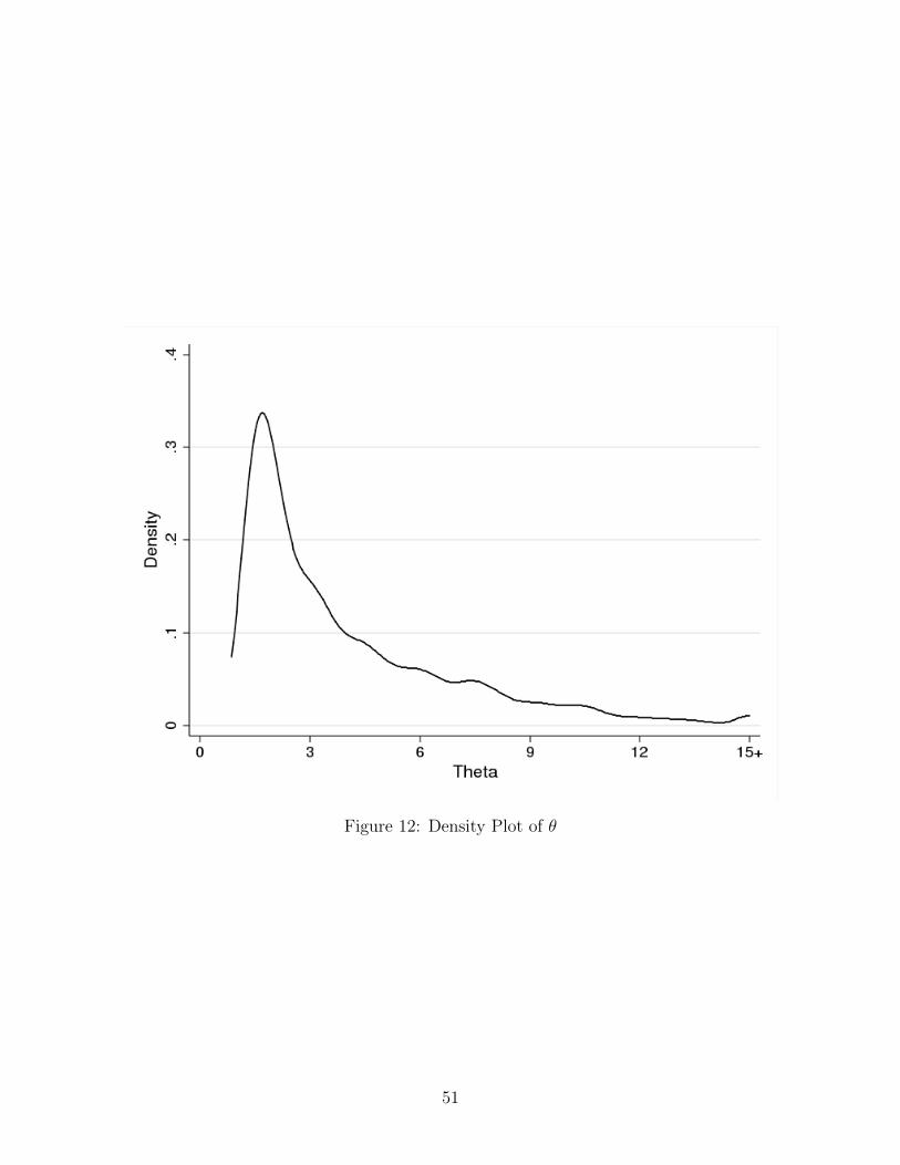
Figure 12: Density Plot of θ

51

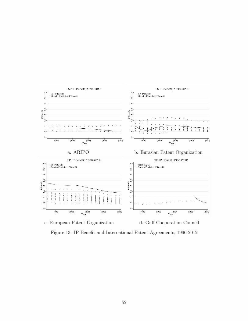
a. ARIPO b. Eurasian Patent Organization

c. European Patent Organization d. Gulf Cooperation Council

Figure 13: IP Benefit and International Patent Agreements, 1996-2012

52

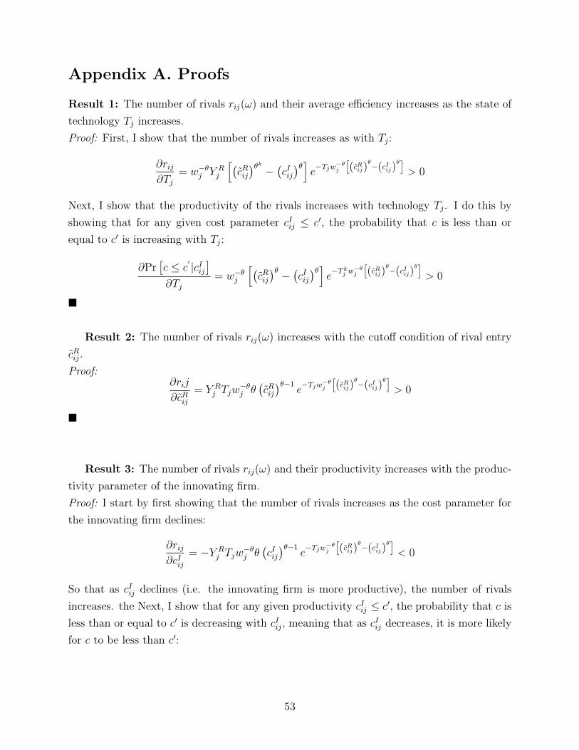
Appendix A. Proofs

Result 1: The number of rivals rij(ω) and their average efficiency increases as the state of

technology Tj increases.

Proof: First, I show that the number of rivals increases as with Tj:

∂rij∂Tj

= w−θj Y Rj

[(cRij)θk − (cIij)θ] e−Tjw−θj [

(cRij)θ−(cIij)

θ]> 0

Next, I show that the productivity of the rivals increases with technology Tj. I do this by

showing that for any given cost parameter cIij ≤ c′, the probability that c is less than or

equal to c′ is increasing with Tj:

∂Pr[c ≤ c

′|cIij]

∂Tj= w−θj

[(cRij)θ − (cIij)θ] e−Tkj w−θj [

(cRij)θ−(cIij)

θ]> 0

Result 2: The number of rivals rij(ω) increases with the cutoff condition of rival entry

cRij.

Proof:∂rij

∂cRij= Y R

j Tjw−θj θ

(cRij)θ−1

e−Tjw−θj

[(cRij)

θ−(cIij)

θ]> 0

Result 3: The number of rivals rij(ω) and their productivity increases with the produc-

tivity parameter of the innovating firm.

Proof: I start by first showing that the number of rivals increases as the cost parameter for

the innovating firm declines:

∂rij∂cIij

= −Y Rj Tjw

−θj θ

(cIij)θ−1

e−Tjw−θj

[(cRij)

θ−(cIij)

θ]< 0

So that as cIij declines (i.e. the innovating firm is more productive), the number of rivals

increases. the Next, I show that for any given productivity cIij ≤ c′, the probability that c is

less than or equal to c′ is decreasing with cIij, meaning that as cIij decreases, it is more likely

for c to be less than c′:

53

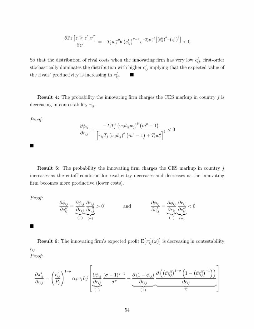
∂Pr[z ≥ z

′ |zI]

∂zI= −Tjw−θj θ

(cIij)θ−1

e−Tjw−θj

[(cRij)

θ−(cIij)

θ]< 0

So that the distribution of rival costs when the innovating firm has very low cIij, first-order

stochastically dominates the distribution with higher cIij implying that the expected value of

the rivals’ productivity is increasing in zIij.

Result 4: The probability the innovating firm charges the CES markup in country j is

decreasing in contestability rij.

Proof:

∂φij∂rij

=−TiT θj (widijwj)

θ (mθ − 1)[

rijTj (widij)θ (mθ − 1

)+ Tiwθj

]2 < 0

Result 5: The probability the innovating firm charges the CES markup in country j

increases as the cutoff condition for rival entry decreases and decreases as the innovating

firm becomes more productive (lower costs).

Proof:∂φij∂cRij

=∂φij∂rij︸︷︷︸(−)

∂rij∂cRij︸︷︷︸(−)

> 0 and∂φij∂cIij

=∂φij∂rij︸︷︷︸(−)

∂rij∂cEij︸︷︷︸(+)

< 0

Result 6: The innovating firm’s expected profit E[πIij(ω)

]is decreasing in contestability

rij.

Proof:

∂πIij∂rij

=

(cIijPj

)1−σ

αjwjLj

∂φij∂rij︸︷︷︸(−)

(σ − 1)σ−1

σσ+∂ (1− φij)

∂rij︸ ︷︷ ︸(+)

∂((mBij

)1−σ(

1−(mBij

)−1))

∂rij︸ ︷︷ ︸??

54

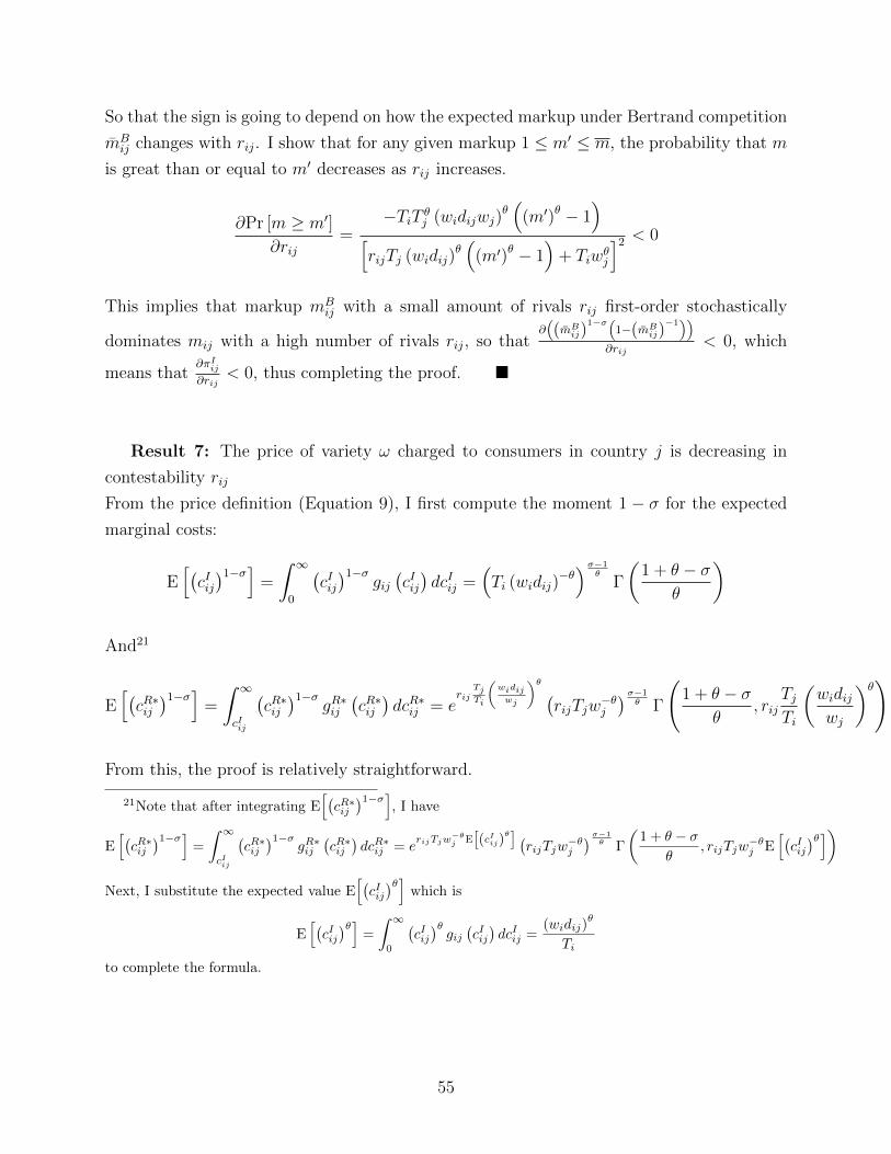
So that the sign is going to depend on how the expected markup under Bertrand competition

mBij changes with rij. I show that for any given markup 1 ≤ m′ ≤ m, the probability that m

is great than or equal to m′ decreases as rij increases.

∂Pr [m ≥ m′]

∂rij=

−TiT θj (widijwj)θ(

(m′)θ − 1)

[rijTj (widij)

θ(

(m′)θ − 1)

+ Tiwθj

]2 < 0

This implies that markup mBij with a small amount of rivals rij first-order stochastically

dominates mij with a high number of rivals rij, so that∂((mBij)

1−σ(1−(mBij)

−1))

∂rij< 0, which

means that∂πIij∂rij

< 0, thus completing the proof.

Result 7: The price of variety ω charged to consumers in country j is decreasing in

contestability rij

From the price definition (Equation 9), I first compute the moment 1 − σ for the expected

marginal costs:

E[(cIij)1−σ

]=

∫ ∞0

(cIij)1−σ

gij(cIij)dcIij =

(Ti (widij)

−θ)σ−1

θΓ

(1 + θ − σ

θ

)

And21

E[(cR∗ij)1−σ

]=

∫ ∞cIij

(cR∗ij)1−σ

gR∗ij(cR∗ij)dcR∗ij = e

rijTjTi

(widijwj

)θ (rijTjw

−θj

)σ−1θ Γ

(1 + θ − σ

θ, rij

TjTi

(widijwj

)θ)

From this, the proof is relatively straightforward.

21Note that after integrating E[(cR∗ij)1−σ]

, I have

E[(cR∗ij)1−σ]

=

∫ ∞cIij

(cR∗ij)1−σ

gR∗ij(cR∗ij)dcR∗ij = e

rijTjw−θj E

[(cIij)

θ] (rijTjw

−θj

)σ−1θ Γ

(1 + θ − σ

θ, rijTjw

−θj E

[(cIij)θ])

Next, I substitute the expected value E[(cIij)θ]

which is

E[(cIij)θ]

=

∫ ∞0

(cIij)θgij(cIij)dcIij =

(widij)θ

Ti

to complete the formula.

55

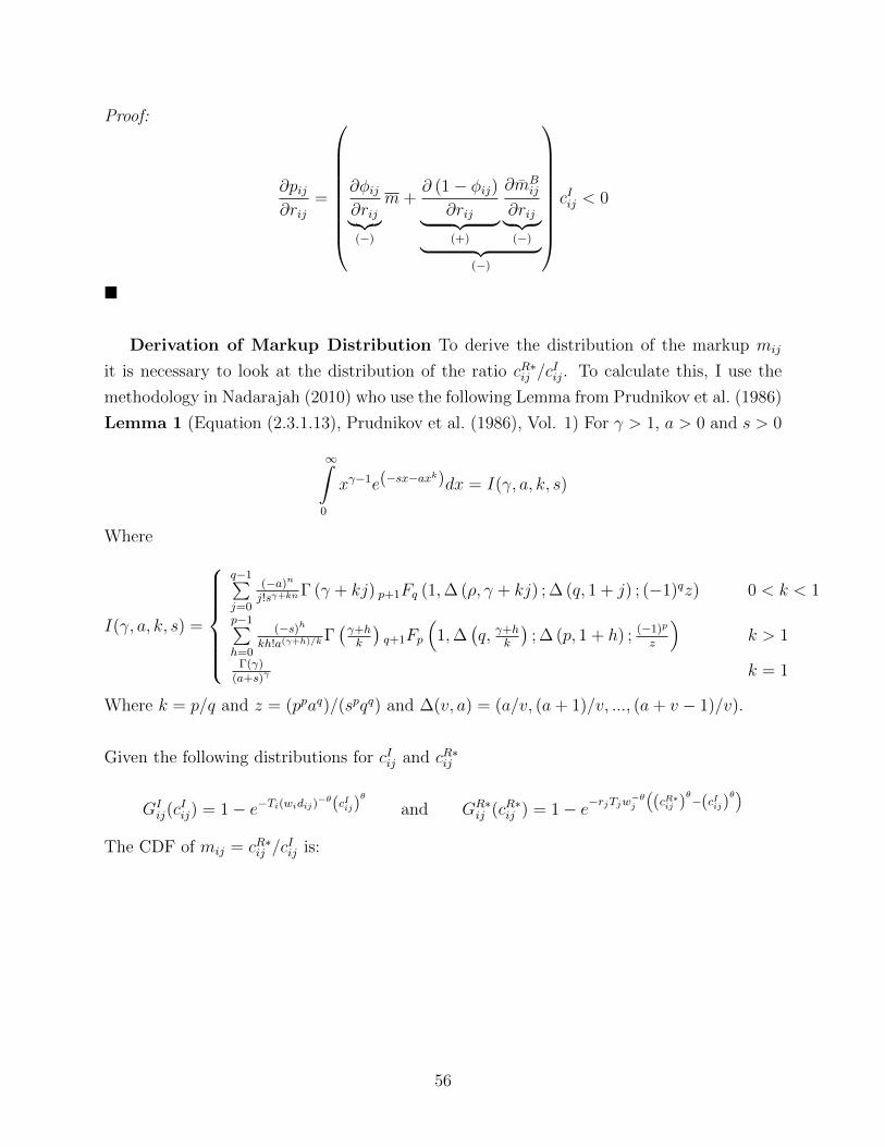
Proof:

∂pij∂rij

=

∂φij∂rij︸︷︷︸(−)

m+∂ (1− φij)

∂rij︸ ︷︷ ︸(+)

∂mBij

∂rij︸ ︷︷ ︸(−)︸ ︷︷ ︸

(−)

cIij < 0

Derivation of Markup Distribution To derive the distribution of the markup mij

it is necessary to look at the distribution of the ratio cR∗ij /cIij. To calculate this, I use the

methodology in Nadarajah (2010) who use the following Lemma from Prudnikov et al. (1986)

Lemma 1 (Equation (2.3.1.13), Prudnikov et al. (1986), Vol. 1) For γ > 1, a > 0 and s > 0

∞∫0

xγ−1e(−sx−axk)dx = I(γ, a, k, s)

Where

I(γ, a, k, s) =

q−1∑j=0

(−a)n

j!sγ+knΓ (γ + kj) p+1Fq (1,∆ (ρ, γ + kj) ; ∆ (q, 1 + j) ; (−1)qz) 0 < k < 1

p−1∑h=0

(−s)h

kh!a(γ+h)/kΓ(γ+hk

)q+1Fp

(1,∆

(q, γ+h

k

); ∆ (p, 1 + h) ; (−1)p

z

)k > 1

Γ(γ)(a+s)γ

k = 1

Where k = p/q and z = (ppaq)/(spqq) and ∆(v, a) = (a/v, (a+ 1)/v, ..., (a+ v − 1)/v).

Given the following distributions for cIij and cR∗ij

GIij(c

Iij) = 1− e−Ti(widij)

−θ(cIij)θ

and GR∗ij (cR∗ij ) = 1− e−rjTjw

−θj

((cR∗ij )

θ−(cIij)

θ)

The CDF of mij = cR∗ij /cIij is:

56

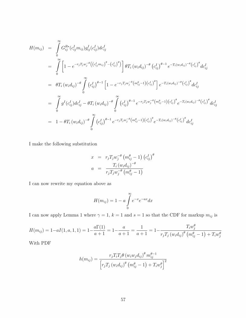
H(mij) =

∞∫0

GR∗ij (cIijmij)g

Iij(c

Iij)dc

Iij

=

∞∫0

[1− e−rjTjw

−θj

((cIijmij)

θ−(cIij)

θ)]θTi (widij)

−θ (cIij)θ−1e−Ti(widij)

−θ(cIij)θ

dcIij

= θTi (widij)−θ

∞∫0

(cIij)θ−1

[1− e−rjTjw

−θj (mθij−1)(cIij)

θ]e−Ti(widij)

−θ(cIij)θ

dcIij

=

∞∫0

gI(cIij)dcIij − θTi (widij)

−θ∞∫

0

(cIij)θ−1

e−rjTjw−θj (mθij−1)(cIij)

θ

e−Ti(widij)−θ(cIij)

θ

dcIij

= 1− θTi (widij)−θ∞∫

0

(cIij)θ−1

e−rjTjw−θj (mθij−1)(cIij)

θ

e−Ti(widij)−θ(cIij)

θ

dcIij

I make the following substitution

x = rjTjw−θj

(mθij − 1

) (cIij)θ

a =Ti (widij)

−θ

rjTjw−θj

(mθij − 1

)I can now rewrite my equation above as

H(mij) = 1− a∞∫

0

e−xe−axdx

I can now apply Lemma 1 where γ = 1, k = 1 and s = 1 so that the CDF for markup mij is

H(mij) = 1−aI(1, a, 1, 1) = 1−aΓ(1)

a+ 1= 1− a

a+ 1=

1

a+ 1= 1−

Tiwθj

rjTj (widij)θ (mθ

ij − 1)

+ Tiwθj

With PDF

h(mij) =rjTiTjθ (wiwjdij)

θmθ−1ij[

rjTj (widij)θ (mθ

ij − 1)

+ Tiwθj

]2

57