International Migration, Human Capital, and Entrepreneurship: Evidence from Philippine Households with Members Working Overseas

Dean Yang∗

Gerald R. Ford School of Public Policy

and Department of Economics, University of Michigan

April 2004

Abstract Millions of households in developing countries receive financial support from family

members working overseas. What impact do overseas economic opportunities have on household investments—in particular, child human capital and household enterprises? Economic theory makes no clear predictions. Overseas income could help households overcome credit constraints that hamper investment. On the other hand, if overseas work is lucrative enough, households could entirely forgo domestic productive activities. This paper sheds light on the impact of overseas economic opportunities on household investment by examining Philippine households’ responses to overseas members’ economic shocks. Overseas Filipinos work in dozens of foreign countries, many of which experienced sudden changes in economic conditions due to the 1997 Asian financial crisis. Identification exploits heterogeneity in the size of migrant shocks across households, using panel household survey data from before and after the shock. Households whose overseas worker(s) experienced more favorable shocks saw differential increases in total household income (mostly via cash transfers from overseas) and in the number of members working overseas. Favorable migrant shocks led to improved child schooling, reduced child labor, increased educational expenditure, and increased durable good ownership (particularly vehicles). Households with more favorable shocks also saw differential increases in hours worked in self-employment, and had larger fluctuations (both positive and negative) in entrepreneurial income. Overseas economic opportunities facilitate investment in migrants’ source households, and may also allow them to engage in riskier entrepreneurial activities. (JEL D13, F22, I2, I3, J22, J23, J24, O12, O15)

∗ Email: deanyang@umich.edu. Address: 440 Lorch Hall, 611 Tappan Street, University of Michigan, Ann Arbor, MI 48109. I have valued feedback from Kerwin Charles, Eric Edmonds, Caroline Hoxby, Larry Katz, Michael Kremer, Sharon Maccini, Justin McCrary, David Mckenzie, Ben Olken, and Dani Rodrik. HwaJung Choi provided excellent research assistance. Research funding was provided by the Social Science Research Council’s Program in Applied Economics, and the MacArthur Network on the Effects of Inequality on Economic Performance.

1 Introduction

Between 1975 and the year 2000, the number of individuals living outside their countries of birth

more than doubled to 175 million, or 2.9% of world population (United Nations (2002)).1 The

remittances that these migrants send to origin countries are an important but relatively poorly-

understood type of international financial flow. According to World Bank data, total workers’

remittances in 1996 amounted to US$58.3 billion worldwide, an amount in excess of total official

development aid in that year, US$49.6 billion.2 An understanding of how these migrant and

remittance flows affect migrants’ origin households is a core element in any assessment of how

international migration affects source countries,3 and in weighing the benefits to source countries

of developed-country policies liberalizing inward migration (as proposed in Rodrik (2002) and

Bhagwati (2003), for example).

What effects do migrant economic opportunities have on migrants’ source households–in

particular, on investments in human capital and productive enterprises? An important body of

research in economics examines the multiple roles migration can play for households in develop-

ing countries (Lucas and Stark (1985), Rosenzweig and Stark (1989), Stark (1991), and Poirine

(1997), among others; see also Taylor and Martin (2001) for an overview). Accumulated migrant

earnings can allow investments that would not have otherwise been made due to credit constraints

and large up-front costs. In addition, insurance provided by distant migrants can allow source

households to engage in riskier income-generating activities (Stark and Levhari (1982)). On the

other hand, the migration of household members may reduce investment, as household members

cannot simultaneously devote time to migrant labor and to investment activities in home areas.

In addition, it is possible that, if migrant work is lucrative enough, household members remaining

behind could entirely forgo productive activities and live primarily on remittance receipts.

Because economic theory makes no clear predictions, empirical work is necessary to determine

the causal impact of migrant economic opportunities on migrants’ source households.4 Many1By contrast, world population grew by just 49% over the same time period (U.S. Bureau of the Census 2002).2The source of these figures is World Bank (2002). While the figure for official development aid is likely to be

relatively accurate, by most accounts (for example, Orozco (2003)) national statistics on workers’ remittances are

considerably underreported. So the 1996 figure of US$58.3 billion can reasonably be taken as a lower bound.3Borjas (1999) argues that the investigation of benefits accruing to migrants’ source countries is an important

and virtually unexplored area in research on migration.4Throughout, this paper emphasizes the impact of ‘migrant economic opportunties’ because of the many chan-

nels (increased remittances, increased insurance, decreased domestic availability of household labor, among others)

through which migration may affect source households.

1

studies find migration and remittance receipts to be positively correlated with various types of

household investments in developing countries.5 By contrast, others argue that resources received

from overseas rarely fund productive investments, and mainly allow higher consumption.6

A central methodological concern with existing work on this topic is that migrant economic

opportunities are in general not randomly allocated across households, so that any observed

relationship between migration or remittances and household outcomes may simply reflect the

influence of unobserved third factors. For example, more ambitious households could have more

migrants and receive larger remittances, and also have higher investment levels. Alternately,

households that recently experienced an adverse shock to existing investments (say, the failure of

a small business) might send members overseas to make up lost income, so that migration and

remittances would be negatively correlated with household investment activity.

An experimental approach to establishing the impact of migrant economic opportunities on

household outcomes could start by identifying a set of households that already had one or more

members working overseas, assigning each migrant a randomly-sized economic shock, and then

examining the relationship between changes in household outcomes and the size of the shock dealt

to the household’s migrants.

This paper takes advantage of a real-world situation akin to the experiment just described.

A non-negligible fraction of households in the Philippines have one or more members working

overseas at any one time.7 These overseas Filipinos work in dozens of foreign countries, many

of which experienced sudden changes in economic conditions due to the 1997 Asian financial

crisis. Most prominently, the crisis led to dramatic exchange rate changes, and–crucially for the

analysis–the changes varied substantially in magnitude across overseas Filipinos’ locations. At

the same time, the Philippine peso also depreciated substantially. The net result was substantial

variation in the size of the exchange rate shock experienced by migrants across source households.

Between July 1997 and October 1998, the US dollar and currencies in the main Middle Eastern

destinations of Filipino workers rose 50% in value against the Philippine peso. Over the same5For example: Brown (1994), Massey and Parrado (1998), McCormick and Wahba (2001), Dustmann and

Kirchkamp (2002), Woodruff and Zenteno (2003), and Mesnard (2004) on entrepreneurship and small business

investment in a variety of countries; Adams (1998) on agricultural land in Pakistan; Cox-Edwards and Ureta (2003)

on child schooling in El Salvador; Taylor, Rozelle, and de Brauw (2003) on agricultural investment in China; and

others.6For example, Lipton (1980), Reichert (1981), Grindle (1988), Massey et al. (1987), and Ahlburg (1991), among

others.7The figure was 6% in June 1997 in the dataset used in this paper.

2

time period, by contrast, the currencies of Taiwan, Singapore, and Japan rose by only 26%, 29%,

and 32%, while those of Malaysia and Korea actually fell slightly (by 1% and 4%, respectively)

against the peso. These depreciations were highly correlated with real economic shocks in affected

countries, so that the change in value of migrant earnings is likely to have been accompanied by

an increased likelihood of overseas job loss. Therefore, throughout this paper I simply use the

exchange rate index as a summary measure of the size of the economic shock faced by overseas

household members.8

Identification exploits this heterogeneity in the size of migrant exchange rate shocks across

households, and examines the association between the size of migrant shocks and changes in

household outcomes. The analysis uses panel household survey data (collected by the Philippine

government) on the household members working overseas, the remittances overseas members send

home, the labor supply and student status of household members, and on detailed household

income and expenditures. Changes are from a period immediately prior to the crisis to a period

15 months later.

Figures 1A through 1D illustrate several of the main findings. Each chart compares two groups

of households: those experiencing exchange rate shocks above and below 0.35, or 35% (a larger

value is a more favorable shock). The black dot is the change in an outcome for households with

a given exchange rate shock; vertical brackets are 95% confidence intervals.

Households whose overseas worker(s) experienced more favorable shocks saw differential in-

creases in cash receipts from overseas (Figure 1A) and in the number of members working over-

seas. Favorable migrant shocks led to improved child schooling, reduced child labor, increased

educational expenditure (Figure 1B), and increased durable good ownership (particularly vehi-

cles). Households with more favorable shocks also saw differential increases in hours worked in

self-employment (Figure 1C), and had larger absolute changes (both increases and decreases) in

entrepreneurial income (Figure 1D). For many outcomes–in particular, the volatility of entrepre-

neurial income–the effect of the shock is smallest among households with the highest pre-crisis

income levels. In sum, overseas economic opportunities facilitate investment in migrants’ source

households, and may also allow them to engage in riskier entrepreneurial activities.

This paper also contributes more broadly to understanding how households in developing

countries respond to changes in economic conditions. The natural experiment exploited in this

paper differs in three ways from existing studies in this area. First, exchange rate shocks faced8I describe the exchange rate index in section 3.2 below.

3

by overseas household members are truly household-specific shocks, rather than locality-level

shocks.9 Second, the size of exchange rate shocks experienced by overseas members is plausibly

uncorrelated with other shocks experienced by the household (omitted variable issues are less of

a concern).10 Third, this paper examines unexpected shocks, unlike studies of anticipated events

such as the receipt of pension income.11

That said, it would not be appropriate to interpret the exchange rate shocks purely as in-

come shocks, because the overseas economic shocks affect migrants’ source households via several

channels: via remittances sent home, via migrants’ location decisions (the decision whether or

not to return home), and via the stock of savings migrants accumulate overseas (which may serve

as insurance for the source household). For this reason, in this paper I do not attempt to use

the exchange rate shock as an instrument for remittance receipts; rather, I focus solely on the

reduced-form impact of the exchange rate shock on a range of household outcomes. The effects

described in this paper should therefore be interpreted simply as the impact on households of an

exogenous change in economic conditions faced by members working overseas.

Section 2 considers the theoretically ambiguous impact of a change in the overseas wage on

household investment decisions. Section 3 describes the dispersion of Filipino household members

overseas, and the nature of the exchange rate shocks. Section 4 presents empirical results, and

section 5 concludes. The Data Appendix describes the household surveys used and procedures9Examples of local-level shocks include weather (Jacoby and Skoufias (1997), Jensen (2000), Rose (1999),

Miguel (2003)) and heterogeneity in the local impact of the 1997 Asian crisis in Indonesia (Frankenberg, Smith,

and Thomas (2003)). These studies credibly establish the causal impact of the shocks in question, but leave open

the possibility that observed changes in household outcomes could be due to changes in local economic variables

(such as wages) rather than household economic conditions per se. Of course, these shocks are also inherently

interesting; the difficulties arise when interpreting their impact as working only through household-level economic

conditions (Rosenzweig and Wolpin (2000)).10Existing studies of the impact of household-level events such as crop loss (Beegle, Dehejia, and Gatti (2003))

or job loss (Duryea, Lam, and Levison (2003)) leave open the concern that unobserved shocks may influence

both the dependent and independent variables. For example, exogenous increases in non-labor income (such as

remittances) might encourage households to engage in riskier work, raising the probability of job loss or crop

failure, and simultaneously raising child schooling and reducing child labor. In this case, the estimated impact of

the independent variable of interest would be biased towards zero.11A number of papers examine the cross-sectional relationship between elderly pension receipt in South Africa

and household outcomes (Case and Deaton (1998), Jensen (1998), Duflo (2003), Bertrand, Mullainathan, and

Miller (2003), Edmonds (2003)). An additional difference between this paper and the South African studies is its

use of panel data, so that bias due to time-invariant heterogeneity correlated with treatment status is less of a

concern.

4

followed for creating the sample for empirical analysis.

2 A model of household investment

In theory, how should improvements in overseas economic conditions affect household investment

activity? When household investments require fixed costs be paid in advance of the investment

returns, and when households face credit constraints, overseas income can affect household invest-

ment decisions. But whether the impact of overseas income on household investment is positive

or negative cannot be predicted in advance based on theory alone.

In sum, household investment activity can be first rising, then falling, in overseas income.

When overseas income is low, higher overseas income can raise households’ willingness to bear

fixed investment costs. Conditional on the household investing, higher overseas incomes can also

encourage households to choose riskier investment activities. Extremely high overseas incomes,

however, could discourage household investment, as households could then choose to live solely

on the overseas income.

I model households deciding whether or not to bear the fixed cost of a household investment

that pays off in a future period. In the second period, households decide how much time to work

in a household entrepreneurial activity. Described in this general way, the household investment

may be literally a business or agricultural activity, but can also encompass investment in the

education of household members.

2.1 Basic elements of the model

Consider a unitary household whose utility depends on leisure and consumption of a market-

purchased good. Due to the existence of fixed investment costs, households face a two-part

decision: decide whether to invest in a household enterprise in the first period; then, if investing,

decide how much time to spend working in the enterprise in the second period.

The household lives for two periods (denoted 1 and 2), and in each period is endowed with T

units of time. In each period, a household has a source of exogenous non-labor income: remittances

from a household member working overseas, in amount R. In addition, let households begin

period 1 with assets A. (The household’s time endowment refers only to members physically in

the household, not to those overseas.)

Households may make an investment in period 1 by paying a fixed cost C. The returns to

5

investment appear in period 2, as earnings from time spent working in the household ‘enterprise’.

Households choose one of two levels of risk for their household enterprise. The risk-free option

earns u per unit of entrepreneurial labor, with certainty. The risky option earns v+ z per unit of

entrepreneurial labor time (v > u), where z is a random and mean-zero productivity shock, with

probability density function f (z).

Let g be the amount of time spent working in the household enterprise in period 2. At the

beginning of period 2 , households must choose which level of risk to take on (risk-free vs. risky),

and their entrepreneurial labor supply g, before discovering the risky entrepreneurial return. So

risk-less entrepreneurial income is ug, while risky entrepreneurial income is (v + z) g.

In period i, household utility depends on its consumption level, xi, and leisure, li (0 ≤ l ≤ T ).For notational simplicity, assume utility in each period is weighted equally (there is no time

discounting), so that the household objective function is simply the sum of utilities in each

period:

U = U (x1, l1) + U (x2, l2) (1)

The utility function has the standard general properties: increasing in each argument, with

negative second partial derivatives. Households maximize this objective function subject to bud-

get and time constraints in each period.

Credit constraints prevent households from transferring resources from the second to the first

period via borrowing, although saving is possible: resources not consumed in period 1 may be

consumed in period 2. Normalize the price of the market-purchased good to 1, so that spending

on the consumption good in period i is xi.

The household determines the optimal use of its time endowment in three cases–without

investment, with risk-free investment, and with risky investment in the household enterprise–

and chooses the option that generates the highest utility. (I assume interior solutions within each

case.)

The no-investment case is straightforward, and symmetric. The household chose not to invest,

so the full time endowment T is taken as leisure in each period: the household simply lives

on income from overseas. To equalize the marginal utility of consumption in each period, the

household consumes R+ A2(overseas income plus half of initial assets) in each period (A

2is saved

from period 1 to 2). Utility is simply 2U³R+ A

2, T´.

6

2.2 The household’s problem, with investment

If the household invests, it chooses either risk-free or risky entrepreneurship, and time spent

working in the entrepreneurial activity in period 2 (g) to maximize utility (equation 1), subject

to budget and time constraints in period 1 and 2 separately. Let us focus on the case where the

fixed investment cost is greater than the household’s starting assets (C > A), in which case the

problem is simplified because there will be no savings (because the marginal utility of consumption

will be higher in period 1 than period 2).

The household determines maximized utility in both the risk-free and risky cases, as follows.

2.2.1 Risk-free investment

In this case, the household’s budget and time constraints are as follows.

l1 ≤ T (period 1 time constraint)

x1 ≤ R+A− C (period 1 budget constraint)l2 ≤ T − g (period 2 time constraint)x2 ≤ R+ ug (period 2 budget constraint)

Substituting these constraints into the objective function yields the following unconstrained

maximization problem:

maxgU (R+A− C, T ) + U (R+ ug, T − g)

Denote the household’s optimal time allocation to entrepreneurial labor in the risk-free in-

vestment case as g∗.

2.2.2 Risky investment

Under risky investment, the household’s budget and time constraints are identical to the risk-free

case, with the exception of the period 2 budget contraint, which is:

x2 ≤ R+ (v + z) g (period 2 budget constraint)

Because the return to entrepreneurial labor in period 2 is subject to the shock z, the household

chooses entrepreneurial labor supply to maximize expected utility:

maxgU (R+A− C, T ) +

ZU (R+ (v + z) g, T − g) f (z) dz

Denote the household’s optimal time allocation to entrepreneurial labor in the risk-free in-

vestment case as g∗∗.

7

2.3 Decision to invest

LetQ∗ be the difference between maximized utility in the risk-free investment case and maximized

utility without investment:

Q∗ ≡ U (R+A− C, T ) + U (R+ ug∗, T − g∗)− 2UµR+

A

2, T¶

Let Q∗∗ be the corresponding difference for the risky investment case:

Q∗∗ ≡ U (R+A− C, T ) +ZU (R+ (v + z) g∗∗, T − g∗∗) f (z) dz − 2U

µR+

A

2, T¶

The household chooses the option that obtains the highest expected utility. Specifically, the

household chooses:Risk-free entrepreneurship if Q∗ ≥ Q∗∗ and Q∗ > 0Risky entrepreneurship if Q∗∗ > Q∗ and Q∗∗ > 0

No entrepreneurship if Q∗∗ ≤ 0 and Q∗∗ ≤ 0What is the impact of overseas income on the household’s decision whether or not to enter

entrepreneurship? Consider the partial derivative of Q∗ with respect to R:

∂Q∗

∂R=

∂U (R+A− C, T )∂R

+∂U (R+ ug∗, T − g∗)

∂R− 2∂U

³R+ A

2, T´

∂R

The first two terms of the expression for ∂Q∗∂R

are positive, and represent the utility gain

(conditional on risk-free entrepreneurship) associated with an increase in overseas income. The

absolute value of the last term in the expression for ∂Q∗∂R

is the utility gain associated with an

increase in overseas income in the no-investment case.

Overall, the sign of ∂Q∗∂R

is ambiguous: the utility gain from risk-free entrepreneurship (versus

no investment) can rise or fall in overseas income. Therefore the impact of a rise in overseas

income on the extensive margin of household entrepreneurial investment cannot be predicted. If

the household was initially not investing (because Q∗ < 0), a rise in overseas income could lead

Q∗ to rise, and the household could be led to invest if it became true that Q∗ > 0. On the other

hand, if the household was initially investing, a rise in overseas income could lead to Q∗ < 0,

leading the household to forgo investment after the wage increase. Similar reasoning holds true

when considering the decision of whether or not to enter risky entrepreneurship.

2.4 A specific example

Assuming a specific functional form for the utility function U and the shock distribution f (z)

allows explicit solutions for the household’s investment decision and entrepreneurial labor supply

(g). Let utility in period i be separable in consumption and leisure,

8

U (xi, li) = (xi)α + γli

where 0 < α < 1. Further, let the probability density function for the entrepreneurial produc-

tivity shock z in the risky case be simply:

f (z) =

v with prob. p

−v with prob. 1− p

Also assume the cost of investment exceeds initial assets (C > A), so that there are no savings.

Optimal entrepreneurial labor supply under risk-free and risky entrepreneurship are (respectively):

g∗ =1

u

µγ

αu

¶ 1α−1 − R

u

g∗∗ =1

2v

Ãγ

2vpα

! 1α−1− R

2v

Graphs for specific parameter values help illustrate the ambiguous effect of overseas income on

the decision to enter entrepreneurship, the level of risk-taking, and entrepreneurial labor supply.

Consider the case where T = 24, α = .5, p = .5, v = 20, u = 6, γ = .5, C = 5, and

A = 1.5. Figure 2A displays utility gains from risk-free and risky entrepreneurship (Q∗ and Q∗∗,

respectively) for values of overseas income R in the interval [1.0,20.0]. At very low and very

high overseas income, the utility gain from entrepreneurship is negative (both lines are below

the horizontal axis); the household chooses not to invest. But at intermediate levels of overseas

income, the utility gain from some type of entrepreneurship is positive, so the household invests.

In addition, higher overseas income can encourage a household to switch from risk-free to risky

entrepreneurship. When the utility gain from risk-free entrepreneurship first becomes greater than

zero (where the thin line, Q∗, first crosses the horizontal axis in Figure 2A), utility from risk-

free entrepreneurship exceeds expected utility from risky entrepreneurship (Q∗ is above Q∗∗, the

thick line). But at slightly higher overseas income, the thin and thick lines cross, so that Q∗∗ is

above Q∗ (and still above the horizontal axis): in this area, risky entrepreneurship yields higher

expected utility than either risk-free entrepreneurship or no entrepreneurship. Households with

high enough overseas income can achieve higher consumption levels regardless of entrepreneurial

income (and so have lower marginal utility of consumption), so that the utility cost of a poor

entrepreneurial income realization is lower. Such households are therefore more willing to take

on entrepreneurial risk.

9

Figure 2B displays optimal entrepreneurial labor supply (g), for overseas income in the same

interval. The line is a step function in overseas income: the optimal labor supply in entrepre-

neurship jumps up discretely (from zero) at the threshold where the household enters risk-free

entrepreneurship (the first step), jumps up again when the household moves from risk-free to risky

entrepreneurship (the second step), and then drops to zero when overseas income is at its highest

level. However, conditional on a certain type of entrepreneurship, incrementally higher overseas

earnings reduce entrepreneurial labor supply on the margin (as reflected in the expressions for g∗

and g∗∗ above). All told, therefore, the amount of entrepreneurial labor supply can either rise or

fall in overseas income, depending on the initial level of overseas income.

In sum, it is clear that the impact of overseas income on household investment and entrepre-

neurial labor supply can be either positive or negative. At very low levels of overseas income,

the marginal utility of consumption in period 1 is so high that households choose not to give up

consumption in that period to invest. An increase in overseas income could move a household

into an intermediate region where investment yields a positive utility gain; higher consumption

is possible in period 1, lowering the cost (in foregone utility) of paying the fixed investment cost

in that period. Large enough increases in overseas income could encourage households to move

into riskier but higher-return entrepreneurial activities. But further increases in overseas income

could push households to the region where investment again is not worthwhile, because high

consumption levels are possible in both periods even without investment.

3 Overseas Filipinos: characteristics and exposure to shocks

3.1 Characteristics of overseas Filipinos

Data on overseas Filipinos are collected in the Survey on Overseas Filipinos (SOF), conducted

in October of each year by the National Statistics Office of the Philippines. The SOF asks a

nationally-representative sample of households in the Philippines about members of the household

who left for overseas within the last five years.

Table 1 displays the distribution of household members working overseas by country in June

1997, immediately prior to the Asian financial crisis.12 Filipino workers are remarkably dispersed12For 90% of individuals in the SOF, their location overseas in that month is reported explicitly. For the

remainder, a few reasonable assumptions must be made to determine their June 1997 location. See the Appendix

for the procedure used to determine the locations of overseas Filipinos in the SOF.

10

worldwide. Saudi Arabia is the largest single destination, with 28.4% of the total, and Hong

Kong comes in second with 11.5%. But no other destination accounts for more than 10% of the

total. The only other countries accounting for 6% or more are Taiwan, Japan, Singapore, and the

United States. The top 20 destinations listed in the table account for 91.9% of overseas Filipino

workers; the remaining 8.1% are distributed among 38 identified countries or have an unspecified

location.

Table 2 displays summary statistics on the characteristics of overseas Filipino workers in the

same survey. 1,832 overseas workers were overseas in June 1997 in the households included in

the empirical analysis (see the Data Appendix for details on the construction of the household

sample). The overseas workers have a mean age of 34.5 years. 38% are single, and 53% are

male. ‘Production and related workers’ and ‘domestic servants’ are the two largest occupational

categories, each accounting for 31% of the total. 31% of overseas workers in the sample have

achieved some college education, and a further 30% have a college degree. In terms of position

in the household, the most common categories are male heads of household and daughters of the

head, each accounting for 28% of overseas workers; sons of head account for 15%, female heads

or spouses of heads 12%, and other relations 16% of overseas workers. As of June 1997, the bulk

of overseas workers had been away for relatively short periods: 30% had been overseas for just

0-11 months, 24% for 12-23 months, and 16% for 24-35 months, 15% for 36-47 months, and 16%

for 48 months or more.

3.2 Shocks generated by the Asian financial crisis

The geographic dispersion of overseas Filipinos meant that there was considerable variety in the

shocks they experienced in the wake of the Asian financial crisis, starting in July 1997. The

devaluation of the Thai baht in that month set off a wave of speculative attacks on national

currencies, primarily (but not exclusively) in East and Southeast Asia.

The shocks generated by the Asian financial crisis affected the real resources of overseas

Filipinos in two ways. First, keeping earnings in foreign currency constant, exchange rate fluctua-

tions changed the Philippine peso value of overseas earnings. Second, many countries experienced

real economic shocks during the financial crisis, so that labor market opportunities of household

members in those countries could have changed, affecting their foreign currency earnings. As

exchange rate shocks in specific countries were highly correlated with the real economic shocks,13

13See Corsetti, Pesenti, and Roubini (1998).

11

I make no attempt to separate these two reasons behind variation in overseas members’ resources,

and simply use an exchange rate index as a summary measure of the size of the shock faced by

overseas household members.

Figure 3 displays monthly exchange rates for selected major locations of overseas Filipinos

(expressed in Philippine pesos per unit of foreign currency, normalized to 1 in July 1996).14 The

sharp trend shift for nearly all countries after July 1997 is the most striking feature of this graph.

An increase in a particular country’s exchange rate should be considered a favorable shock to

an overseas household member in that country: each unit of foreign currency earned would be

convertible to more Philippine pesos once remitted, and should also have been associated with

better economic conditions in the country.

For each country j, I construct the following measure of the exchange rate change between the

year preceding July 1997 and the year preceding October 1998:

ERCHANGEj =Average country j exchange rate from Oct. 1997 to Sep. 1998Average country j exchange rate from Jul. 1996 to Jun. 1997

− 1. (2)

A 50% improvement would be expressed as 0.5, a 50% decline as -0.5. Exchange rate changes

for the 20 major destinations of Filipino workers are listed in the third column of Table 1. The

changes for the major Middle Eastern destinations and the United States were all at least 0.50.

By contrast, the exchange rate shocks for Taiwan, Singapore, and Japan were 0.26, 0.29, and

0.32, while for Malaysia and Korea they were actually negative: -0.01 and -0.04, respectively.

Workers in Indonesia experienced the worst exchange rate change (-0.54), while those in Libya

experienced the most favorable change (0.57) (not shown in table).

I construct a household-level exchange rate shock variable as follows. Let the countries in the

world where overseas Filipinos work be indexed by j ∈ {1, 2, ..., J}. Let nij indicate the numberof overseas workers a household i has in a particular country j in June 1997 (so that

PJj=1 nij is

its total number of household workers overseas in that month). The exchange rate shock measure

for household i is:

ERSHOCKi =

PJj=1 nijERCHANGEjPJ

j=1 nij(3)

In other words, for a household with just one worker overseas in a country j in June 1997, the

exchange rate shock associated with that household is simply ERCHANGEj. For households

with workers in more than one foreign country in June 1997, the exchange rate shock associated

with that household is the weighted average exchange rate change across those countries, with14The exchange rates are as of the end of each month, and were obtained from Bloomberg L.P.

12

each country’s exchange rate weighted by the number of household workers in that country.15

In addition, the Philippine economy experienced a decline in economic growth after the onset

of the crisis. Annual real GDP contracted by 0.8% in 1998, as compared to growth of 5.2% in 1997

and 5.8% in 1996 (World Bank 2002). The urban unemployment rate (unemployed as a share of

total labor force) rose from 9.5% to 10.8% between 1997 and 1998, while the rural unemployment

rate went from 5.2% to 6.9% over the same period (Philippine Yearbook (2001), Table 15.1). Any

effects of the domestic economic downturn common to all sample households (as well as effects of

the crisis that differ according to households’ observed pre-crisis characteristics) will be accounted

for in the empirical analysis, as described in the next section.

4 Empirics: impact of migrant shocks on households

In this section, I describe the data and sample construction, the characteristics of sample house-

holds, the regression specification and some empirical issues, and then present empirical results.

4.1 Data and sample construction

The empirical analysis uses data from four linked household surveys conducted by the National

Statistics Office of the Philippine government, covering a nationally-representative household

sample: the Labor Force Survey (LFS), the Survey on Overseas Filipinos (SOF), the Family

Income and Expenditure Survey (FIES), and the Annual Poverty Indicators Survey (APIS).

The LFS is administered quarterly to inhabitants of a rotating panel of dwellings in January,

April, July, and October, and the other three surveys are administered with lower frequency as

riders to the LFS. Usually, one-fourth of dwellings are rotated out of the sample in each quarter,

but the rotation was postponed for five quarters starting in July 1997, so that three-quarters of

dwellings included in the July 1997 round were still in the sample in October 1998 (one-fourth of

the dwellings had just been rotated out of the sample). The analysis of this paper takes advantage

of this fortuitous postponement of the rotation schedule to examine changes in households over

the 15-month period from July 1997 to October 1998.

Survey enumerators note whether the household currently living in the dwelling is the same as

the household surveyed in the previous round; only dwellings inhabited continuously by the same15Of the 1,646 households included in the analysis, 1,485 (90.2%) had just one member working overseas in June

1997. 140 households (8.5%) had two, 18 households (1.1%) had three, and three households (0.2%) had four

members working overseas in that month.

13

household from July 1997 to October 1998 are included in the sample for analysis.16 Because the

research question of interest is the impact of shocks experienced by migrants on outcomes in the

migrants’ source households, households are only included in the sample for empirical analysis

if they reported having one or more members overseas in June 1997 (immediately prior to the

Asian financial crisis). The survey does not include unique identifiers for surveyed individuals;

for analysis of individual outcomes, individuals must be matched over time (within households)

on the basis of age and gender.

See the Data Appendix for details regarding the contents of the surveys, the construction of

the sample for analysis, and the procedure for matching individuals across survey rounds.

4.2 Characteristics of sample households

Table 3 presents summary statistics for the 1,646 households used in the empirical analysis. The

top row displays summary statistics for the exchange rate shock. The mean change in the shock

index was 0.41, with a standard deviation of 0.16.

The mean number of household overseas workers in June 1997 is 1.11. Median cash receipts

from overseas was 26,000 pesos (US$1,000) in Jan-Jun 1997. Pre-crisis cash receipts from overseas

were substantial as a share of household income, with a median of 0.37.

Households in the sample tend to be wealthier than other Philippine households in terms of

their initial (Jan-Jun 1997) income per capita. 51% of sample households are in the top quartile of

the national household income per capita distribution, and 28% are in the next-highest quartile.

Median pre-crisis (Jan-Jun 1997) household expenditures is 57,544 Philippine pesos (US$2,213),

median pre-crisis household income is 70,906 pesos (US$2,727).17 Median pre-crisis income per

capita in the household is 15,236 pesos (US$586). Mean pre-crisis household size is 6.16 members

(including overseas members).18 68% of sample households are urban, compared to the national

figure of 59%.

Reflecting the importance of remittances from overseas, sample households tend to rely less

on wage/salary, entrepreneurial, and agricultural income than the typical Philippine household.16As discussed in the Data Appendix (and illustrated in Appendix Table 2), there is no evidence that attrition

from the sample between July 1997 and October 1998 is correlated with a household’s exchange rate shock.17When I report US dollars, they are converted from Philippine pesos at the first-half 1997 exchange rate of

roughly 26 pesos per US$1.18The corresponding pre-crisis (Jan-Jun 1997) national medians (for all households) are as follows: household

expenditure, 33,647 pesos; household income, 37,362 pesos; income per capita, 7,944 pesos. The national mean

household size in July 1997 is 5.27.

14

The mean of pre-crisis wage and salary income as a share of total income is 0.23 (compared with

a national average of 0.41). The mean of pre-crisis entrepreneurial income as a share of total

income is 0.17 (compared with a national average of 0.31). 50 percent of sample households have

nonzero entrepreneurial income, compared with a national average of 59 percent. The mean of

pre-crisis agricultural income as a share of total income is 0.10 (compared with a national average

of 0.27).

Only 23 percent of sample household heads work in agriculture, compared with a national

average of 37 percent. The heads of the households in this sample are relatively highly educated:

52 percent have at least a high school education. (The national average is 40 percent.) The mean

age of household heads in this sample is 49.9, compared with 46.9 nationally.

4.3 Regression specification

In investigating the impact of exchange rate shocks on changes in outcome variables between 1997

and 1998, a first-differenced regression specification is natural:

∆Yit = β0 + β1 (ERSHOCKi) + δ0 (Xit−1) + εit (4)

For household i, ∆Yit is the change in an outcome of interest. ERSHOCKi is the exchange

rate shock for household i, as defined above in (3). First-differencing of household-level vari-

ables is equivalent to the inclusion of household fixed effects in a levels regression; time-invariant

differences across households in outcome variables are accounted for.

The constant term, β0, accounts for the average change in outcomes across all households in the

sample. This is equivalent to including a year fixed effect in a regression where outcome variables

are expressed in levels (not changes), and accounts for the shared impact across households of

the decline in Philippine economic growth after the onset of the crisis.

Xht−1 is a vector of household location indicators and control variables for pre-shock household

characteristics.19 εht is a mean-zero error term. Standard errors are clustered according to the19Household location fixed effects are 16 indicators for regions within the Philippines and their interactions

with an indicator for urban location. Household-level controls are as follows. Income variables as reported in

Jan-Jun 1997: log of per capita household income; indicators for being in 2nd, 3rd, and top quartile of the

sample distribution of household per capita income. Demographic and occupational variables as reported in July

1997: number of household members (including overseas members); five indicators for head’s highest level of

education completed (elementary, some high school, high school, some college, and college or more; less than

elementary omitted); head’s age; indicator for ‘head’s marital status is single’; six indicators for head’s occupation

15

June 1997 location of overseas worker.20

The coefficient of interest is β1, the impact of a unit change in the exchange rate shock on

the outcome variable. The identification assumption is that if the exchange rate shocks faced

by households had all been of the same magnitude (instead of varying in size), then changes in

outcomes would not have varied systematically across households on the basis of their overseas

workers’ locations.

If migrant shocks were truly assigned to households randomly, the vector of pre-crisis household

characteristics Xht−1 should be uncorrelated with changes in outcomes. Including these variables

in the regression would simply pick up changes in outcomes associated with initial characteristics

(for reasons unconnected to the exchange rate shocks), potentially reducing residual variation and

leading to more precise coefficient estimates on the exchange rate shock variable.

In addition, examining whether regression results change when the pre-crisis household charac-

teristics are included in the regression is a partial test of the parallel-trend identification assump-

tion. An important type of violation of the parallel-trend assumption would be if households

experiencing more favorable shocks were different along certain pre-shock characteristics from

households experiencing less favorable shocks, and if changes in outcomes would have varied

along those same characteristics even in the absence of the migrant shocks.

In fact, households experiencing more favorable migrant shocks do differ along a number of

pre-shock characteristics from households experiencing less-favorable shocks. Appendix Table

1 presents coefficient estimates from a regression of the household’s exchange rate shock on a

number of pre-shock characteristics of households and their overseas workers. Several individual

variables are statistically significantly different from zero, indicating that households experienced

more favorable exchange rate shocks if they had fewer members, heads who were more educated,

less educated migrants, and migrants who had been away for longer periods prior to the crisis.

F-tests reject the null that some subgroups of variables are jointly equal to zero: indicators

(professional, clerical, service, production, other, not working; agricultural omitted).

Migrant controls are means of the following variables across household’s overseas workers away in June 1997:

indicators for months away as of June 1997 (12-23, 24-35, 36-47, 48 or more; 0-11 omitted); indicators for highest

education level completed (high school, some college, college or more; less than high school omitted); occupation

indicators (domestic servant, ship’s officer or crew, professional, clerical, other service, other occupation; production

omitted); relationship to household head (female head or spouse of head, daughter, son, other relation; male head

omitted); indicator for single marital status; years of age.20For households that had more than one overseas worker overseas in June 1997, the household is clustered

according to the location of the eldest overseas worker.

16

for household per capita income percentiles; indicators for household head’s education level;

indicators for household geographic location in the Philippines; overseas workers’ months away

variables; overseas workers’ education variables; and overseas workers’ occupation variables.

These initial differences would be problematic if they were associated with differential changes

in outcomes independent of the exchange rate shocks. For example, suppose that the domestic

economic downturn caused small household enterprises to be more likely to fail in households

with less-educated heads, so that entrepreneurial incomes rise differentially for better-educated

households than for less-educated households in the wake of the crisis. Appendix Table 1 indicates

that households with better-educated heads also experienced more-favorable exchange rate shocks.

Then the estimated impact of the exchange rate shocks on household entrepreneurial income would

be biased upwards.

Including the vector of pre-crisis household characteristics Xht−1 when estimating equation

4 helps control for changes in outcome variables related to households’ pre-crisis characteristics.

Examining whether coefficient estimates on the exchange rate shock variable change when the

pre-crisis household characteristics are included in the regression can shed light whether changes

in outcome variables related to these characteristics are correlated with households’ exchange rate

shocks, constituting a partial test of the parallel-trend identification assumption.

In most results tables, I therefore present regression results with and without the vector

of controls for pre-crisis household characteristics, Xht−1. In nearly all cases, inclusion of the

initial household characteristics controls makes little difference to the coefficient estimates, and

on occasion actually makes the coefficient estimates larger in absolute value (suggesting that, in

these cases, changes in outcome variables related to households’ pre-crisis characteristics bias the

estimated effect of the shock towards zero). Inclusion of these pre-crisis characteristics controls

also often reduces standard errors on the exchange rate shock coefficients.

4.4 Regression results

This subsection examines the impact of household exchange rate shocks on the following out-

comes in sequence: remittance receipts and overseas work; household income and expenditures;

household durable good ownership; child schooling, and adult and child labor supply by type of

work; entrepreneurial labor supply and entrepreneurial income in more detail; and a number of

detailed expenditure items. At the end, I also examine heterogeneity in the impact of the shocks

by pre-crisis household per capita income quartile.

17

4.4.1 Remittance receipts and overseas work

Table 4 presents coefficient estimates from estimating equation (4) when the outcome variables

are the change in cash receipts, gifts, etc. from overseas (remittances) and the household’s

number of overseas workers.21 For comparison, the table also presents regression results where

the outcome is the change in cash receipts, gifts, etc. from domestic sources. The change in

cash receipts variables are changes between the January-June 1997 and April-September 1998

reporting periods, divided by pre-crisis (January-June 1997) household income. (For example, a

change amounting to 10% of initial income is expressed as 0.1.)22

Each cell of the table presents the coefficient estimate on the exchange rate shock variable in

a separate regression. The first column presents regression results without the inclusion of any

other right-hand-side variables, while the second column includes household location fixed effects

and the control variables for pre-crisis household and migrant characteristics. (This format–

presenting regression results with and without control variables alongside each other–will be

followed in most subsequent regression results tables.)

The coefficients on the exchange rate shock in the regressions for cash receipts from overseas

are positive in both specifications, and larger in absolute value (36% larger) and more precisely

measured when control variables are included (in column 2). It seems that households experiencing

more favorable exchange rate shocks also have pre-shock characteristics that are associated with

declines in remittances over the study period; controlling for these characteristics raises the

estimated impact of the exchange rate shock on remittances. As should be expected, there is no

relationship between the exchange rate shock and cash receipts from domestic sources (the shock

coefficients are very small and are not statistically signficantly different from zero).

The coefficients on the exchange rate shock in the regressions for number of overseas workers

are positive, and similar in magnitude across the two specifications (the estimate in column

2 is just 7% smaller than the estimate in column 1). The coefficients are highly statistically

significantly different from zero on both specifications.

The coefficients on the exchange rate shock in the second column indicate that a one-standard-

deviation increase the size of the exchange rate shock (0.16) is associated with a differential21For a more detailed theoretical and empirical treatment of overseas workers’ return decisions in these house-

holds, see Yang (2003).22Dividing by pre-crisis household income is a normalization to take account of the fact that households in the

sample have a wide range of income levels, and allows coefficient estimates to be interpreted as fractions of initial

household income.

18

increase in remittances of 3.8 percentage points of pre-shock (Jan-Jun 1997) household income,

and a differential decline of 0.043 in the number of overseas workers in the household.

4.4.2 Household income and expenditures

Table 5 presents coefficient estimates on the exchange rate shock when the outcome variables

are total household income and its major components, and total household expenditures and its

major components. Changes in income (expenditure) items are changes between the January-

June 1997 and April-September 1998 reporting periods, divided by pre-crisis (January-June 1997)

household income (expenditures).

The coefficients on the exchange rate shock in the regressions for total household income are

positive in both specifications, and essentially the same in absolute value (within 1% in size) and

more precisely measured when control variables are included (in column 2). Essentially all of the

impact of the shock on total household income comes through the change in the ‘other sources

of income’ category, which includes cash receipts from overseas. In turn, the impact of the shock

on ‘other sources of income’ appears to work entirely through the change in cash receipts from

overseas: the coefficients and significance levels in the regressions for other sources of income (in

Table 5) are essentially the same as those for cash receipts from overseas (in Table 4).

The estimated impacts of the exchange rate shocks on wage and salary income and on entre-

preneurial income are small in magnitude and not statistically significantly different from zero

in all specifications. The coefficients on total household expenditures, food expenditures, and

non-food expenditures are actually negative in sign, but all are modest in size and none are

statistically significantly different from zero. There is no evidence that household consumption

expenditures at these aggregate levels were substantially affected by shocks to migrants.

The coefficients on the exchange rate shock in the second column indicate that a one-standard-

deviation increase the size of the exchange rate shock (0.16) is associated with a differential

increase in total household income of 4.2 percent of pre-shock (Jan-Jun 1997) household income.

4.4.3 Durable good ownership

Table 6 presents coefficient estimates on the exchange rate shock when the outcome variables are

changes in an indicator for household ownership of six specific durable goods: radio, television,

living room set, dining set, refrigerator, and vehicle. The outcome variables take on the values

19

-1, 0, and 1.23

The coefficients on the exchange rate shock in all regressions except for refrigerators are

positive. In the specification without control variables (the first column), the coefficients for

television and vehicle ownership are statistically significantly different from zero at conventional

levels (respectively, the 10% and 1% levels). In the specification with control variables (the second

column), the coefficients for television, living room set, and vehicle ownership are statistically

significantly different from zero at conventional levels (respectively, the 1%, 10%, and 1% levels).

For ownership of televisions and living room sets, the coefficients become substantially larger

and attain higher levels of statistical significance in the specifications with control variables.

In the regression for vehicle ownership, the coefficient becomes slightly smaller in absolute

value, falling in magnitude by 14%. It appears that households experiencing more favorable

exchange rate shocks also have pre-shock characteristics that are associated with increases in ve-

hicle ownership over the study period. Controlling for these characteristics reduces the estimated

impact of the exchange rate shock on vehicle ownership, but the estimate remains substantial in

magnitude and statistically significantly different from zero.

The coefficients on the exchange rate shock in the second column indicate that a one-standard-

deviation increase the size of the exchange rate shock (0.16) is associated with a differential

increase in the likelihood of television, living room set, and vehicle ownership of 1.5, 0.9, and 2.3

percentage points, respectively.

4.4.4 Labor supply by type of work, and child schooling

This section describes the impact of exchange rate shocks on labor supply by type of work at the

household level, and then turns to changes in schooling and labor supply by type of work at the

individual level.

4.4.4.1 Household-level labor supply by type of work Table 7 presents coefficient esti-

mates on the exchange rate shock when the outcome variables are changes in total hours worked

and changes in hours worked in different types of employment in the week prior to the survey.

The coefficients on the exchange rate shock in the regressions for total hours worked are positive23As described in the Data Appendix, durable good ownership data were not recorded in July 1997, so changes

in the ownership indicators are between January 1998 and October 1998. If durable good ownership changed

by January 1998 in response to the July-December 1997 economic shocks experienced by migrants, the empirical

estimates reported for these outcomes are likely to be lower bounds of the true effects.

20

but not statistically significantly different from zero. The same is true in regressions for hours

worked for employers outside the household.

More favorable exchange rate shocks are associated with increases in hours worked in self em-

ployment: the coefficients in these regressions are positive and statistically significantly different

from zero. In the specification with control variables (column 2), the coefficient estimate becomes

19% larger in absolute value and attains the 5% significance level, compared with the specification

without controls (column 1).

The coefficient on the exchange rate shock in the second column indicates that a one-standard-

deviation increase the size of the exchange rate shock (0.16) is associated with a differential

increase in hours worked in self employment of 1.6 hours per week.

There is also suggestive evidence that hours worked without pay in family-operated farms or

businesses declines with more favorable exchange rate shocks (the coefficients for this outcome

are negative in sign and relatively large in magnitude), but these results are not statistically

significantly different from zero. It may be that better migrant economic conditions are associated

with differential shifts out of work without pay and into self employment in household enterprises.

4.4.4.2 Individual-level schooling and labor supply by type of work: children and

young adults Table 8 presents coefficient estimates on the exchange rate shock when the

outcome variables are individual-level changes in student status, total hours worked and hours

worked in different types of employment in the week prior to the survey. The ‘student indicator’

variable is the change in an indicator for ‘student’ being the person’s reported primary activity

between July 1997 and October 1998 (this variable takes on the values -1, 0, and 1). In the

analysis of hours worked by type of employment, a combined category for ‘hours worked in self

employment, as an employer, or as a worker with pay in a family-operated farm or business’ is

used, because children and young adults are reported to work very few hours in these types of

employment separately.

Results are presented separately for females aged 10-17, males aged 10-17, females aged 18-24,

and males aged 18-24. For each subgroup results are presented for specifications with and without

control variables. Control variables for pre-crisis characteristics include the same household and

migrant variables used in previous tables, and also include pre-crisis individual characteristics:

fixed effects for each year of age; a gender indicator, indicator for single marital status, indicator for

‘student’ being the person’s primary activity, indicator for ‘not in labor force’, and five indicators

for highest schooling level completed (elementary, some high school, high school, some college,

21

and college or more).

The coefficients on the exchange rate shock in the regressions for the student indicator are

all positive in sign, and are statistically significantly different from zero in the specifications with

control variables for females aged 10-17 and males aged 18-24. In three out of the four subsamples,

the coefficient on the shock is larger in absolute value in the specification with control variables.

(The exception is for females aged 18-24; in this case standard errors are very large in both

specifications.)

For children aged 10-17, the coefficients on the exchange rate shock in the regressions for

total hours worked all negative in sign, and the coefficient is statistically significantly different

from zero in the specification with control variables for males. For both males and females in

this age group, more favorable exchange rate shocks lead to statistically significantly fewer hours

of work without pay in family enterprises. For males, more favorable exchange rate shocks lead

to statistically significant increases in hours worked in self employment, as an employer, or as a

worker with pay in a family-operated farm or business, but this increase is not large enough to

offset the overall decline in hours worked for this subgroup. For all statistically significant results

among children aged 10-17, the magnitude of the estimated coefficient is larger in absolute value

in specifications with control variables than in specifications without control variables.

For young adults aged 18-24, the statistically significant results for hours worked are confined

to males, and are somewhat nuanced. Total hours worked and hours worked for employers outside

the household decline for males in households with more favorable shocks, but coefficient estimates

are not statistically significantly different from zero. More favorable exchange rate shocks lead

males to supply statistically significant increases in hours worked in self employment, as an

employer, or as a worker with pay in a family-operated farm or business, and to equally large

and statistically significant declines in hours worked without pay in family enterprises. Again, for

both these statistically significant results, the magnitude of the estimated coefficient is larger in

absolute value in specifications with control variables than in those without.

In sum, more favorable shocks are associated with more schooling for children and young adults

of both genders. The coefficient on the exchange rate shock in regressions with control variables

indicate that a one-standard-deviation increase in the size of the exchange rate shock (0.16) is

associated with a differential increase in the likelihood of being a student of 2.1 percentage points

for females aged 10-17, and 3.5 percentage points for males aged 18-24. For children aged 10-17,

more favorable shocks are associated with declines in total hours worked, in particular for males:

male hours worked in the past week in this age group declines differentially by 0.52 hours per

22

week in households experiencing one-standard-deviation-larger exchange rate shocks.

For male young adults (aged 18-24), a one-standard-deviation increase the size of the exchange

rate shock is associated with a differential increase in hours worked for pay in family enterprises

of 1.3 hours per week, and a decline in hours worked without pay of roughly the same magnitude.

4.4.4.3 Individual-level labor supply by type of work: adults Table 9 presents regres-

sion results for labor supply by type of work in the past week for adults (aged 25-64), separately

for females and males. Specifications are similar to those in Table 8, but for these individuals it

is possible to examine changes in hours worked in more disaggregated work categories. Control

variables are also the same as those in Table 8.

For both genders, the coefficients on the exchange rate shock in the regressions for total hours

worked all positive in sign, but no coefficient is statistically significantly different from zero. There

is no evidence here that better overseas economic prospects substantially reduce the labor supply

of adults in migrants’ source households.

For males, more favorable exchange rate shocks lead to statistically significant increases in

hours worked in self employment, and in hours worked with pay in a family-operated farm or

business (but the latter coefficient is substantially smaller in absolute value). In the regressions

for hours worked in self employment, the magnitude of the estimated coefficient is larger in

absolute value (by 28%) in the specification with control variables than in the specification without

them; the opposite is true in the regression for hours worked with pay in a family-operated

farm or business (the coefficient becomes 26% smaller), but the coefficient remains statistically

significantly different from zero.

For females, more favorable exchange rate shocks lead to statistically significant (at the 10%

significance level) decreases in hours worked as an employer in a family enterprise, but this

coefficient is relatively small in magnitude.

For males, the coefficient on the exchange rate shock in regressions with control variables

indicate that a one-standard-deviation increase the size of the exchange rate shock (0.16) is

associated with a differential increase in hours worked in self employment of 1.4 hours per week,

and a concurrent differential increase for of 0.15 hours per week in hours worked with pay in

a family-operated farm or business. For females, a similarly-sized positive exchange rate shock

leads to a decline of 0.3 hours worked per week as an employer in a family enterprise.

A possible explanation for these patterns is that in households experiencing differential im-

provements in migrants’ economic conditions, male household members devote differentially more

23

hours to working in their own enterprise, with some of this increase coming at the expense of

hours worked for the enterprises of female household members.

4.4.5 Entrepreneurial labor supply and entrepreneurial income: further detail

This section examines in further detail the impact of the exchange rate shock on entrepreneurial

(self employment) hours worked and entrepreneurial income. It explores the impact of the shock

on the volatility of entrepreneurial income (aside from its level). In addition, it asks whether the

exchange rate shocks act on the extensive or intensive margins of entrepreneurship by separately

examining two subsamples of households: households with some pre-crisis entrepreneurial income,

and households with no pre-crisis entrepreneurial income. Finally, it examines what types of

entrepreneurial income appear to be most highly affected by the exchange rate shocks.

Table 10 presents results from household-level regressions examining the impact of exchange

rate shocks on entrepreneurial (self-employment) labor supply and entrepreneurial income, for all

households and separately for the two subsamples. Results for all households are presented in the

first two columns (for specifications without and with control variables), and corresponding pairs

of results for the two subsamples are displayed in the subsequent four columns.

4.4.5.1 Volatility of entrepreneurial income Focusing for the moment on regression re-

sults for all sample households (in the first two columns of Table 10), the top row of the table

repeats the coefficient estimates for the change in total household hours worked in self employment

from Table 7, and the second row repeats the coefficient estimates for the change in entrepreneur-

ial income from Table 5. At first blush, it is somewhat puzzling that more-favorable exchange

rate shocks raise household hours worked in self employment but do not raise household entre-

preneurial income.

As it turns out, the primary effect of more-favorable exchange rate shocks on household

entrepreneurial income is to raise its volatility, rather than its level. The outcome variable in the

third row of the table is the absolute value of the change in entrepreneurial income (as a fraction

of pre-crisis total household income); the positive and statistically significant coefficient on the

exchange rate shock in the regression with control variables indicates that households with more

favorable exchange rate shocks experience larger changes in entrepreneurial income, both positive

and negative.

The remaining rows of the table demonstrate that this conclusion also holds when examining

binary outcomes: indicators for households experiencing a 25% increase in entrepreneurial income

24

(row 4), a 25% decrease in entrepreneurial income (row 5), and either a 25% increase or decrease in

entrepreneurial income (row 6) (all changes are with respect to pre-crisis household income). All

coefficient estimates in the regression with control variables are positive in sign, and those for the

25% increase (row 4) and either a 25% increase or decrease (row 6) are statistically significantly

different from zero (at the 10% and 5% levels, respectively). For all these binary outcomes, the

coefficient estimates are more positive when control variables are included in the regression.

These results may reflect the fact that more favorable economic conditions for migrants allow

source households to engage in riskier productive activities. Households whose migrants experi-

ence worse shocks may reduce their exposure to entrepreneurial risk by differentially reducing their

labor supply in such activities, and therefore experience smaller fluctuations in entrepreneurial

incomes.

4.4.5.2 Impact on households with and without pre-crisis entrepreneurial income

Examining whether and how the impact of the exchange rate shocks on entrepreneurial labor

supply and entrepreneurial income differ across households with and without pre-crisis entre-

preneurial income can shed light on whether the exchange rate shocks act on the extensive or

intensive margins of entrepreneurship.

For all outcomes in Table 10, when the regressions are estimated for the subsample of house-

holds with pre-crisis entrepreneurial income (columns 3 and 4), the coefficients on the exchange

rate shocks become larger in absolute value than when the regression is estimated using all sample

households (columns 1 and 2). By contrast, the coefficients on the exchange rate shock in the

regressions for households without pre-crisis entrepreneurial income (columns 5 and 6) become

substantially smaller and closer to zero. (No results are reported for households without pre-crisis

entrepreneurial income in rows 3, 5, and 6 because it is not possible for entrepreneurial income

to decline for this subsample.)

The impact of migrant shocks on household entrepreneurial labor supply and entrepreneurial

income appears to operate entirely on the intensive margin of entrepreneurship: the shocks only

affect households in these areas if they had some entrepreneurial activity to start with. In terms

of the theoretical model of section 2, favorable exchange rate shocks could be thought of as

increases in overseas income that move households from the area of risk-free to risky investment.

As illustrated in Figures 2A and 2B, such a movement would result in higher entrepreneurial

labor supply, and (by definition) more volatile entrepreneurial income.

The coefficients on the exchange rate shock for households with some pre-crisis entrepreneurial

25

income in regressions with control variables (column 4) indicate that a one-standard-deviation

increase the size of the exchange rate shock (0.16) is associated with an increase in hours worked

in self employment of 2.2 hours in the past week, a change (either positive or negative) in entre-

preneurial income of 2.8 percentage points of pre-crisis household income, and an increase of 3.9

percentage points in the likelihood that the household’s entrepreneurial income changes either

positively or negatively by more than 25% (of pre-crisis household income).

4.4.5.3 Impact on entrepreneurial income, by source Table 11 examines the impact

of exchange rate shocks on changes in different sources of entrepreneurial income, focusing on

households with nonzero pre-crisis entrepreneurial income. The first two columns of the table

present regression results for the simple change in income, and the last two columns are for the

absolute value of the change in income by source (as before, all changes are expressed as fractions

of pre-crisis total household income).

In the first two columns, the results for income from transport, storage, and communication

services stand out. In specifications with and without control variables, the coefficients on the

exchange rate shock are positive and highly statistically significantly different from zero. The

coefficient is larger in magnitude when control variables are included in the regression. A one-

standard-deviation increase the size of the exchange rate shock (0.16) is associated with an increase

in income from this entrepreneurial source of 1.3 percentage points of pre-crisis total household

income. It is possible that this result is related to the differential increase in the likelihood of

vehicle ownership experienced by households with more favorable shocks. Households may be

using newly-acquired vehicles for provision of transport services.

In addition, households experiencing more favorable exchange rate shocks see differential

declines in income from ‘community, social, and recreational and personal services’ (the coef-

ficient for this outcome is statistically significantly different from zero at the 10% level in the

specification with control variables). A one-standard-deviation increase the size of the exchange

rate shock (0.16) is associated with a decline in income from this entrepreneurial source of 0.5

percentage points of pre-crisis total household income. It is possible that households experiencing

more favorable shocks may be switching out of this activity to alternative entrepreneurial activ-

ities, or they may be taking on more risk in this activity that happened to result in losses over

the study period.

The third and fourth columns of the table present results for the absolute value of the change

in income by entrepreneurial source. More favorable exchange rate shocks are associated with

26

statistically significant changes (both positive and negative) in income from wholesale and re-

tail activities. A one-standard-deviation increase the size of the exchange rate shock (0.16) is

associated with an absolute change in income from this entrepreneurial source of 1.4 percentage

points of pre-crisis total household income. It is possible that better economic opportunities for

a household’s migrants allow households to take on more risk in this activity.

4.4.6 Detailed expenditure items

The point estimates of the impact of exchange rate shock on household expenditures (from Table

5) provide no indication that aggregate expenditure levels were affected systematically by the

shocks. However, there is evidence that households changed the composition of their expenditures

somewhat in response to the shocks. This section discusses regression results where outcomes are

the change in household expenditures on detailed items, where changes are expressed as fractions

of pre-crisis (Jan-Jun 1997) household expenditures.

Table 12 examines changes in food expenditures. While the shocks do not have a substantial

effect on either food at home or food outside the home (coefficient estimates for these outcomes

are close to zero and statistically insignificant), they do seem to lead to small reallocations of

food expenditures. More favorable shocks lead to statistically significantly higher expenditures

on ‘cereals and cereal preparation’ and on ‘coffee, cocoa and tea’, and to statistically significantly

lower expenditures on ‘fish and marine products’.

Table 13 examines changes in non-food expenditures. Exchange rate shocks lead to statistically

significant declines in the value of housing services and in expenditure on ‘special family occasions’.

These results may be related to the fact that more favorable shocks lead to differential increases

in the number of household members overseas. Households with fewer domestic residents need

less housing (rooms may be rented out to boarders, for example).24 Expenditures by overseas

workers home on vacation are included in special family occasions, so this result may indicate

that favorable shocks make overseas workers become less likely to return home on vacation.

More favorable shocks also lead to statistically significant differential increases in expenditures

on education and on ‘gifts and contributions to others’. The education result is consistent with the

finding (in Table 8) of differential increases in student status in households with more favorable

shocks. The result for gifts to others is intriguing, and suggests that the benefits from migrants’

overseas opportunities extend beyond the migrants’ source households.24This result should not indicate that households are moving to smaller dwellings, because households are not

included in the sample if they change dwellings between the July 1997 and October 1998 surveys.

27

4.4.7 Heterogeneity in impact of shocks by pre-crisis income group

How do the impacts of the shocks vary by pre-crisis income group? Table 14 examines how

the impact of the exchange rate shocks on several outcome variables differs across households

in each quartile of the distribution of pre-crisis per capita income in the sample households, by

interacting the exchange rate shock with indicators for whether the household is in each quartile.

The coefficient on each interaction term provides the estimated impact of the exchange rate shock

for households in the given quartile.

The first column examines heterogeneity in the impact of the exchange rate shock on the

change in household hours worked in self-employment for households with some pre-crisis entre-

preneurial income. The coefficients are statistically significant (at the 10% level) for households

in the middle two quartiles and larger in magnitude than the coefficients in either the bottom

(first) or top (fourth) quartiles, but none of the differences among the coefficients are statistically

significantly different from zero.

The regression in the second column is specified identically to the first column’s regression,

except that the outcome is the absolute value of the change in household hours worked in self-

employment. The coefficients are statistically significant for households in the first three quartiles

and are all larger in magnitude than the coefficient for the top (fourth) quartile. An F-test rejects

the null hypothesis that the coefficient for the middle-to-high income group is the same as the

same as the coefficient for the high income group at the 1% significance level. The coefficient

for the low income group also differs from the coefficient for the high income group at the 10%

significance level. This pattern would emerge if the lower-income households required better

migrant economic conditions before taking on more entrepreneurial risk in the wake of the crisis,

perhaps because of credit constraints that bind more for the lower-income households.

In column 3, the outcome is the change in vehicle ownership and the regression is estimated

for all households. Exchange rate shocks have the strongest relationship with the likelihood of

vehicle ownership for households in the middle two income groups. An F-test rejects the null

hypothesis that the coefficient for the middle-to-high income group is the same as the same as the

coefficient for the low income group at the 1% significance level. It may be that the lowest-income

households are too far from the threshold for vehicle purchase for the migrant shocks to affect

their decisions on this margin.

Columns 4 and 5 present regression results for individual-level regressions where the outcomes

are the change in student status for children aged 10-17. For both genders, large and statistically

28

significant effects are concentrated in one of the middle-income groups: for females in this age

range, the largest effects are for the middle-to-high income group, while for males, the largest

effects are for the low-to-middle income group. Due to the size of standard errors, however, it is

not possible to reject the null at conventional significance levels that any of the coefficients on

the interaction terms in the same regression are identical to each other.

It is useful to understand whether the patterns just described in columns 1-5 are due to

differential impacts of exchange rate shocks on migrant returns and remittances for households

in the different income groups. Columns 6 and 7 present regression results for household-level

regressions where the outcomes are the change in the number of household overseas workers and

the change in cash receipts from overseas. While coefficients are largest and achieve the highest

levels of statistical significance in the middle-income groups, coefficient estimates are not close to

zero for any income group and F-tests do not reject the null at conventional significance levels

that any of the coefficients on the interaction terms in either column are identical to each other.

In sum, the patterns of effects by income group in Table 14 suggest that the impacts of the

exchange rate shocks on household investment are smallest among the highest-income house-

holds. A possible explanation is that such households have greater access to credit and insurance

mechanisms.

5 Conclusion

Due to their locations in a wide variety of countries, overseas Filipino workers were exposed to

economic shocks of various sizes in the wake of the Asian financial crisis. The crisis thus generated

substantial variation in overseas economic opportunities across these migrants’ source households

in the Philippines. This paper takes advantage of this unusual natural experiment to identify the

impact of overseas economic opportunities on a range of outcomes in Philippine households, such

as child schooling, child labor, and entrepreneurial activity.

Migrants’ economic opportunities facilitate investment in source households, and may also

allow them to engage in riskier entrepreneurial activities. Households whose overseas members

faced more favorable shocks saw increases in remittance receipts, increases in child schooling,

increases in educational expenditure, declines in child labor, increases in hours worked in entre-

preneurial activities, and changes (both positive and negative) in entrepreneurial income. For

many outcomes–in particular, the volatility of entrepreneurial income–the effect of the shock is

smallest among households with the highest pre-crisis income levels.

29

In future work, it will be important to explore why investment seems less responsive to mi-

grant economic opportunities in higher-income households. Possible explanations include greater

availability of credit and insurance mechanisms for such households.

This paper also demonstrates the possibility of exploring the impact of international migration

on households in developing countries using existing datasets collected by national governments.

The Philippines is not likely to be the only country whose national household survey includes

questions on international migration and remittances, and so valuable future work could seek

evidence in other countries of the impacts of economic shocks faced by migrants on outcomes in

the migrants’ source households.

6 Data appendix

6.1 Data sets

Four linked household surveys were provided by the National Statistics Office of the Philippine

government: the Labor Force Survey (LFS), the Survey on Overseas Filipinos (SOF), the Family

Income and Expenditure Survey (FIES), and the Annual Poverty Indicators Survey (APIS).25

The Labor Force Survey (LFS) collects data on primary activity (including ‘student’), hours

worked in the past week, and demographic characteristics of household members aged 10 or above.

These data refer to the household members’ activities in the week prior to the survey. The survey

defines a household as a group of people who live under the same roof and share common food.

The definition also includes people currently overseas if they lived with the household before

departure. As collected in the LFS, hours worked refers only to work for pay or profit, whether

outside or within the household, or work without pay on a family farm or enterprise; it excludes

housekeeping and repair work in one’s own home.

The Survey on Overseas Filipinos (SOF) is administered in October of each year to households

reporting in the LFS that any members left for overseas within the last five years. The SOF collects

information on characteristics of the household’s overseas members, their overseas locations and

lengths of stay overseas, and the value of remittances received by the household from overseas in

the last six months (April to September).

In the analysis, I use the July 1997 and October 1998 rounds of the LFS and the October 1997

and October 1998 rounds of the SOF. Because 1997 remittances in the SOF refer to an April-25Use of the data requires a user fee, and the datasets remain the property of the Philippine government.

30

September reporting period, the SOF remittance data cannot be used to determine a household’s

level of remittances prior to the July 1997 Asian financial crisis. So I obtain data on cash receipts

from overseas from the Family Income and Expenditure Survey (FIES), which was conducted in

July 1997 and January 1998. This dataset records all household income sources (including cash

receipts from overseas) separately for January to June 1997 and July to December 1997, neatly

dividing the year into pre- and post-crisis halves. I obtain a household’s initial (Jan-Jun 1997)

remittances from the FIES.

Data on detailed income sources and expenditures are available for the pre-crisis period (Jan-

Jun 1997) from the July 1997 FIES. Data on detailed income sources, expenditures, and durable

good ownership are available for the post-crisis period (Apr-Sep 1998) from the October 1998

Annual Poverty Indicators Survey (APIS). Unfortunately, data on durable good ownership and

housing unit amenities in the pre-crisis period is unavailable in the July 1997 round of the FIES;

these data were only recorded in the January 1998 survey. So analyses of changes in assets

examine changes from January 1998 (from the FIES) to October 1998 (from the APIS). To the

extent that durable good ownership already changed by January 1998 in response to migrant

shocks, the empirical estimates reported for these outcomes are likely to be lower bounds of the

true effects.

Data on cash receipts from overseas (remittances) in the second reporting period (Apr-Sep

1998) are available in both the APIS and the SOF (both conducted in October 1998). All analyses

of cash receipts from overseas use data from the SOF for the second reporting period because

this source is likely to be more accurate (the SOF asks for information on amounts sent by each

household member overseas, which are then added up to obtain total remittance receipts; by

contrast, the APIS simply asks for total cash receipts from overseas). Total household income in

Apr-Sep 1998 (obtained from the APIS) is adjusted so that the remittance component reflects

data from the SOF.

Monthly exchange rate data (used in constructing the exchange rate shock variable) were

obtained from Bloomberg L.P.

The sample used in the empirical analysis consists of all households meeting the following

criteria:

1. The household is inferred to have one or more members working overseas in June 1997.

Using the October 1997 SOF, I identify households that had one or more members working

overseas in June 1997, and identify the locations of these overseas members. (See the next

31

subsection for the exact procedure.)

2. The household’s dwelling was also included in the October 1998 LFS/SOF. As mentioned

above, one-quarter of households in the sample in July 1997 had just been rotated out of

the sample in October 1998.

3. The same household has occupied the dwelling between July 1997 and October 1998. This

criterion is necessary because the Labor Force Survey does not attempt to interview house-

holds that have changed dwellings. Usefully, the LFS dataset contains a field noting whether

the household currently living in the dwelling is the same as the household surveyed in the

previous round.

4. The household has complete data on pre-crisis control and outcome variables (recorded July

1997).

5. The household has complete data on post-crisis outcome variables (recorded October 1998).

Of 30,744 dwellings that the National Statistics Office did not rotate out of the sample be-

tween July 1997 and October 1998 (criterion 2), 28,152 (91.6%) contained the same household

continuously over that period (criterion 3). Of these households, 27,768 (98.6%) had complete

data for all variables used in the analysis (criteria 4 and 5). And of these 27,768, 1,646 (5.9%)

had a member overseas in June 1997 (criterion 1). These 1,646 households are the sample used

in the empirical analysis.

Constructing the sample on the basis of Criteria 1, 2, and 4 does not threaten the validity of

the empirical estimate of the impact of the migrant economic shocks on households. Criteria 1

and 4 are based on pre-shock characteristics of the surveyed households, and criterion 2 comes

from the predetermined rotation schedule established by the National Statistics Office.

It is important to check whether sample selection on the basis of Criteria 3 or 5 may have

been affected by the independent variable of interest (shocks experienced by migrant members)

because household propensities to change dwellings or to misreport information in the survey

may have been affected by the shocks. Attrition from the household sample due to these criteria

should not generate biased coefficient estimates if such attrition is uncorrelated with the shocks.

Appendix Table 2 (Part A) presents results from household-level regressions where the de-

pendent variable is an indicator for attrition from the sample due to Criteria 3 or 5. The sample

in the regression is all households satisfying Criteria 1, 2, and 4. 5.6% of households satisfying

32

Criteria 1, 2, and 4 fail to satisfy either Criteria 3 or 5. The reported coefficient is that on

the migrant exchange rate shock variable. The regression controls for location fixed effects and

pre-crisis household and overseas worker characteristics (see Table 4 for a list of these control

variables). The coefficient is not statistically significantly different from zero and is very small

in magnitude (.008). There is no indication that attrition due to Criteria 3 or 5 is associated

with the shocks, and so allowing these criteria play a role in determining the sample for analysis

should not threaten the internal validity of the estimates.

6.2 Determining pre-crisis location of overseas household members

In this subsection I describe the rules used to determine if a particular individual in the October

1997 Survey on Overseas Filipinos was overseas in June 1997, and if so, what country the person

was in. Among other questions, the SOF asks:

1. When did the family member last leave for overseas?

2. In what country did the family member intend to stay when he/she last left?

3. When did the family member return home from his/her last departure (if at all)?

These questions unambiguously identify individuals as being away in June 1997 (and their

overseas locations) if they left for overseas in or before that month, and returned afterwards (or

have not yet returned). Unfortunately, the survey does not collect information on stays overseas

prior to the most recent one. So there are individuals who most recently left for overseas between

June 1997 and the survey date in October 1997, but who were likely to have been overseas before

then as well. Fortunately, there is an additional question in the SOF that is of use:

4. How many months has the family member worked/been working abroad during the last

five years?

Using this question, two reasonable assumptions allow me to proceed. First, assume all stays

overseas are continuous (except for vacations home in the midst of a stay overseas). Second,

assume no household member moves between countries overseas. When making these two as-

sumptions, the questions asked on the SOF are sufficient to identify whether a household had a

member in a particular country in June 1997.

For example, a household surveyed in October 1997 might have a household member who

last left for Saudi Arabia in July 1997 and had not yet returned from that stay overseas. If

that household member is reported as having worked overseas for 4 months or more, the first

assumption implies the person first left for overseas in or before June 1997. The second assumption

33

implies that the person was in Saudi Arabia.

89.8% of individuals identified as being away in June 1997 (and their overseas locations) were

classified as such using just questions 1 to 3 above. The remaining 10.2% of individuals identified

as being away in June 1997 (and their locations) relied on question 4 above and the two allocation

assumptions just described.26

6.3 Matching individuals across survey rounds

In the surveys used in the empirical analysis, it is possible to follow households over time as long

as they remain in the same dwelling. However, these data do not explicitly track individuals

across survey rounds (there is no unique identifier for individuals). Therefore, when the outcome

of interest in the empirical analysis is a change at the individual level (individual schooling and

labor supply), I match individuals within households between the July 1997 and October 1998

survey rounds using individuals’ reported age and gender.

Because closer relatives of the household head should be more likely to remain resident in the

household between the two survey rounds (and thus should generate a higher-quality match), I

limit the samples in each period to household heads and the spouses, children, and parents of

household heads. I first look for ‘perfect matches’, matches between individuals in the two survey

rounds who have the same gender, and where the individual observed in October 1998 reports

being one year older (age t+ 1) than the person observed in July 1997 (age t).

Because there is likely to be substantial reporting/measurement error in age, I also allow

‘imperfect matches’: matches between an individual observed in July 1997 (age t) and the same-

gendered individual in the household in October 1998 who is closest in to the July 1997 individual’s

age plus one (closest to age t+1). For individuals aged 25 and above in July 1997 (where t ≥ 25),I allow such imperfect matches if the matched person’s age in October 1998 is no more than 5

years different from age t+ 1. Younger people are likely to have better-reported ages, and so for

individuals aged 10-24 in July 1997 (where 10 ≤ t ≤ 24), I allow imperfect matches only if thematched person’s age in October 1998 is no more than 2 years different from age t+1. I make no

attempt to match individuals below the age of 10 in July 1997, as no data is collected on these

individuals for the outcome variables of interest.

Whenever more than one match occurs for a particular individual within a household (if26Empirical results are not substantially affected when analyses are conducted only on the households where all

overseas workers are unambiguously assigned to overseas locations using questions 1, 2, and 3 above.

34

one individual in July 1997 matches with two or more individuals in the same household in

October 1998, or if more than one person in the household in July 1997 has the same age-

gender combination), I do not attempt to resolve the match ambiguity and simply drop the given

household from the sample altogether. These situations are rare, and in any case should be

uncorrelated with migrant exchange rate shocks.

As a quality check, I make sure matched individuals’ education level and reported marital sta-

tus across the two survey rounds are reasonable: I disallow matches where individuals’ education

levels change by more than two levels between the two rounds, and matches where individuals

change in marital status from being married or formerly-married in July 1997 to single in October

1998. Over 96% of potential matches pass these checks.

Of all individuals observed in July 1997, 81% of individuals aged 25 and above and 68% of

individuals aged 10-24 were matched with an individual in the same household in October 1998

using the procedure just described. These figures include attrition of entire households (due

to Criteria 3 and 5 described in Appendix section 6.1 above) as well as unsuccessful individual

matches. The successful matches used in the empirical analysis are roughly evenly split between

‘perfect’ and ‘imperfect’ matches.

Attrition from the individual-level sample (due to failed matches) should not generate biased

coefficient estimates if attrition is random with respect to the independent variable of interest, the

migrant exchange rate shock. Indeed, there is no indication that the incidence of failed matches

is associated with these shocks among individuals who would have been included in the sample

for analysis if not for the failed match. Appendix Table 2 presents results from individual-level

regressions where the dependent variable is an indicator for attrition from the sample due to

failed matching, in three age groups (10-17, 18-24, and 25-64) for males and females separately.

(Individuals are included in this regression if the individual’s household satisfied Criteria 1, 2,

and 4, as described in Appendix section 6.1 above, and if the individual had complete data on

individual characteristics in July 1997.) Reported coefficients are those on the migrant exchange

rate shock. All regressions control for location fixed effects and pre-crisis individual, household,

and overseas worker characteristics. None of the coefficients are statistically significantly different

from zero, and both positive and negative coefficients occur (depending on the sub-sample).

35

7 References

Adams, Richard H., Jr., ‘Remittances, Investment, and Rural Asset Accumulation in Pak-

istan,’ Economic Development and Cultural Change, Vol. 17, No. 1, 1998, pp. 155-173.

Ahlburg, Dennis, Remittances and Their Impact : A Study of Tonga and Western Samoa.

Canberra: National Centre for Development Studies, Research School of Pacific Studies, the

Australian National University, 1991.

Beegle, Kathleen, Rajeev H. Dehejia, and Roberta Gatti, ‘Child Labor, Crop Shocks, and

Credit Constraints’, NBER Working Paper 10088, November 2003.

Bertrand, Marianne, Sendhil Mullainathan, and Doug Miller, ‘Public Policy and Extended

Families: Evidence from Pensions in South Africa,’ World Bank Economic Review, Vol. 17, No.

1, 2003.

Bhagwati, Jagdish, ‘Borders Beyond Control,’ Foreign Affairs, Vol. 82 (1), January/February

2003, pp. 98-104.

Borjas, George, ‘The Economic Analysis of Immigration,’ in Orley Ashenfelter and David

Card, eds., Handbook of Labor Economics, Vol. 3A, North-Holland, 1999, pp. 1697-1760.

Brown, Richard P.C., ‘Migrants’ Remittances, Savings, and Investment in the South Pacific’,

International Labour Review, Vol. 133, No. 3, 1994, pp. 347-367.

Case, Anne and Angus Deaton, ‘Large Cash Transfers to the Elderly in South Africa,’ Eco-

nomic Journal, Vol. 108, September 1998, pp. 1330-1361.

Corsetti, Giancarlo, Paolo Pesenti, and Nouriel Roubini, ‘What Caused the Asian Currency

and Financial Crisis? Part II: The Policy Debate,’ NBER Working Paper 6834, December 1998.

Cox-Edwards, Alexandra and Manuelita Ureta, ‘International Migration, Remittances, and

Schooling: Evidence from El Salvador,’ Journal of Development Economics, Vol. 72, 2003, pp.

429-461.

Duflo, Esther, ‘Grandmothers and Granddaughters: Old Age Pension and Intra-Household

Allocation in South Africa,’ World Bank Economic Review, Vol. 17, No. 1, 2003.

36

Duryea, Suzanne, David Lam, and Deborah Levison, ‘Effects of Economic Shocks on Children’s

Employment and Schooling in Brazil,’ Population Studies Center Research Report No. 03-541,

Institute for Social Research, University of Michigan, December 2003.

Dustmann, Christian, and Olivier Kirchkamp, ‘The Optimal Migration Duration and Activity

Choice After Re-migration,’ Journal of Development Economics, Vol. 67, 2002, pp. 351-372.

Edmonds, Eric, ‘The Response of Child Labor Supply to Anticipated Income,’ mimeo, Dart-

mouth College Department of Economics, 2003.

Frankenberg, Elizabeth, James P. Smith, and Duncan Thomas, ‘Economic Shocks, Wealth,

and Welfare,’ Journal of Human Resources, 2003.

Grindle, Merilee, Searching for Rural Development: Labor Migration and Employment in

Mexico. Ithaca: Cornell University Press, 1988.

Jacoby, Hanan, and Emmanuel Skoufias, ‘Risk, Financial Markets, and Human Capital in a

Developing Country,’ Review of Economics and Statistics, Vol. 64, 1997, pp. 311-335.

Jensen, Robert, ‘Public Transfers, Private Transfers, and the ‘Crowding Out’ Hypothesis:

Evidence From South Africa,’ Kennedy School of Government Faculty Research Working Paper

#R98-08, 1998.

Jensen, Robert, ‘Agricultural Volatility and Investments in Children,’ American Economic

Association Papers and Proceedings, May 2000, pp. 399-404.

Lipton, Michael, ‘Migration from rural areas of poor countries: The impact on rural produc-

tivity and income distribution’, World Development, Vol. 8, No. 1, January 1980, pp. 1-24.

Lucas, Robert E.B., and Oded Stark, ‘Motivations to Remit: Evidence from Botswana,’ Jour-

nal of Political Economy, Vol. 93, No. 5, 1985, pp. 901-918.

Massey, Douglas S., Raul Alarcon, Jorge Durand, and H. Gonzalez, Return to Aztlan: The

Social Process of International Migration fromWestern Mexico. Berkeley: University of California

Press, 1987.

Massey, Douglas S. and Emilio A. Parrado, ‘International Migration and Business Formation

in Mexico,’ Social Science Quarterly, Vol. 79, No. 1, March 1998, pp. 1-19.

37

McCormick, Barry and Jackline Wahba, ‘Overseas Work Experience, Savings and Entrepre-

neurship Amongst Return Migrants to LDCs,’ Scottish Journal of Political Economy, Vol. 48,

No. 2, May 2001, pp. 164-178.

Mesnard, Alice, ‘Temporary Migration and Capital Market Imperfections,’ Oxford Economic

Papers, Vol. 56, 2004, pp. 242-262.

Miguel, Edward, ‘Poverty and Witch Killing,’ BREAD Working Paper No. 041, August 2003.

Orozco, Manuel, ‘Worker remittances: an international comparison,’ working paper, Inter-

American Development Bank, February 2003.

Philippine Yearbook, Manila: National Statistics Office, 2001.

Poirine, Bernard, ‘A Theory of Remittances as an Implicit Family Loan Arrangement,’World

Development, Vol. 25, No. 4, 1997, pp. 589-611.

Reichert, J., ‘The Migrant Syndrome: Seasonal US Wage Labor and Rural Development in

Central Mexico,’ Human Organization, Vol. 40, No. 1, pp. 56-66.

Rodrik, Dani, ‘Globalization for Whom?’ Harvard Magazine, Vol. 104 (6), July-August 2002,

p.29.

Rose, Eliana, ‘Consumption Smoothing and Excess Female Mortality in Rural India,’ Review

of Economics and Statistics, Vol. 81, No. 1, 1999, pp. 41-49.

Rosenzweig, Mark and Oded Stark, ‘Consumption Smoothing, Migration, and Marriage: Ev-

idence from Rural India,’ Journal of Political Economy, Vol. 97, No. 4, 1989, pp. 905-926.

Rosenzweig, Mark and Kenneth Wolpin, ‘Natural ‘Natural Experiments’ in Economics,’ Jour-

nal of Economic Literature, Vol. 38, December 2000, pp. 827-874.

Stark, Oded, The Migration of Labor. Oxford: Basil Blackwell, 1991.

Stark, Oded and David Levhari, ‘On Migration and Risk in LDCs,’ Economic Development

and Cultural Change, 1982, pp. 191-196.

Taylor, J. Edward and Philip L. Martin, ‘Human Capital: Migration and Rural Population

Change,’ in Bruce L. Gardner and Gordon C. Rausser, eds. Handbook of Agricultural Economics,

Volume 1A. Amsterdam: Elsevier Science, North-Holland, 2001, pp. 457-511.

38

Taylor, J. Edward, Scott Rozelle, and Alan de Brauw, ‘Migration and Incomes in Source

Communities: A New Economics of Migration Perspective from China,’ Economic Development

and Cultural Change, 2003.

United Nations, International Migration Report 2002, UN Population Division, New York.

United States Bureau of the Census, International Data Base, Washington, D.C., 2002.

Woodruff, Christopher and Rene Zenteno, ‘Remittances and Microenterprises in Mexico,’

mimeo, University of California, San Diego and ITESM, 2003.

World Bank, World Development Indicators on CD-ROM 2002, Washington, D.C.

Yang, Dean, ‘The Dynamics of International Labor Migration: Understanding the Departure

and Return of Overseas Filipino Workers,’ mimeo, University of Michigan, 2003.

39

Table 1 Locations of overseas workers from sample households(June 1997)

LocationNumber of

overseas workers % of totalExchange rate

shock(June 1997-Oct 1998)

Saudi Arabia 521 28.4% 0.52Hong Kong, China 210 11.5% 0.52Taiwan 148 8.1% 0.26Singapore 124 6.8% 0.29Japan 116 6.3% 0.32United States 116 6.3% 0.52Malaysia 65 3.5% -0.01Italy 52 2.8% 0.38Kuwait 51 2.8% 0.50United Arab Emirates 49 2.7% 0.52Greece 44 2.4% 0.30Korea, Rep. 36 2.0% -0.04Northern Mariana Islands 30 1.6% 0.52Canada 29 1.6% 0.42Brunei 22 1.2% 0.30United Kingdom 15 0.8% 0.55Qatar 15 0.8% 0.52Norway 14 0.8% 0.35Australia 14 0.8% 0.24Bahrain 13 0.7% 0.52Other 148 8.1%

Total 1,832 100.0%

NOTES -- Data are from Oct 1997 Survey of Overseas Filipinos. "Other" includes 38 additional countries plus a category for "unspecified" (total 58 countries explicitly reported). Overseas workers in table are those in households included in sample for empirical analysis (see Data Appendix for details on sample definition). Exchange rate shock: Change in Philippine pesos per currency unit where overseas worker was located in Jun 1997. Change is average of 12 months leading to Oct 1998 minus average of 12 months leading to Jun 1997, divided by the latter (e.g., 10% increase is 0.1).

afc_tables summstats_ows_locations

Table 2 Characteristics of overseas workers from sample households

Mean Std. Dev. 10th pctile Median 90th pctile

Age 34.49 9.00 24.00 33.00 47.00

Marital status is single (indicator) 0.38

Gender is male (indicator) 0.53

Occupation (indicators)Production and related workers 0.31Domestic servants 0.31Ship's officers and crew 0.12Professional and technical workers 0.11Clerical and related workers 0.04Other services 0.10Other 0.01

Highest education level (indicators)Less than high school 0.15High school 0.25Some college 0.31College or more 0.30

Position in household (indicators)Male head of household 0.28Female head or spouse of head 0.12Daughter of head 0.28Son of head 0.15Other relation to head 0.16

Months overseas as of Jun 1997 (indicators)0-11 months 0.3012-23 months 0.2424-35 months 0.1636-47 months 0.1548 months or more 0.16

Number of individuals: 1,832

NOTE -- Data source is October 1997 Survey of Overseas Filipinos, National Statistics Office of the Philippines. "Other" occupational category includes "administrative, executive, and managerial workers" and "agricultural workers". Overseas workers in table are those in households included in sample for empirical analysis (see Data Appendix for details on sample definition).

afc_tables summstats_ows

Table 3 Initial characteristics of sample householdsNum. of obs.: 1,646

Mean Std. Dev. 10th pctile Median 90th pctile

Exchange rate shock (see below for definition) 0.41 0.16 0.26 0.52 0.52

Household financial statistics (Jan-Jun 1997)Total expenditures 73,596 66,529 24,600 57,544 132,793Total income 94,272 92,826 28,093 70,906 175,000Income per capita in household 20,235 21,403 5,510 15,236 39,212Cash receipts from overseas 36,194 46,836 0 26,000 87,500Cash receipts from overseas (as share of hh income) 0.40 0.31 0.00 0.37 0.85

Number of household members working overseas in Jun 1997 1.11 0.36 1 1 1Household size (including overseas members, Jul 1997) 6.16 2.42 3 6 9Located in urban area 0.68

HH position in national income per capita distribution, Jan- Jun 1997 (indicators)

Top quartile 0.513rd quartile 0.282nd quartile 0.14Bottom quartile 0.07

HH income sources (Jan-Jun 1997)Wage and salary, as share of total 0.23 0.29 0.00 0.07 0.68Indicator: nonzero wage and salary income 0.53Entrepreneurial income, as share of total 0.17 0.25 0.00 0.00 0.58Indicator: nonzero entrepreneurial income 0.50Agricultural income, as share of total 0.10 0.21 0.00 0.00 0.42Indicator: nonzero agricultural income 0.50

Household head characteristics (Jul 1997):Age 49.9 13.9 32 50 68Highest education level (indicators)

Less than elementary 0.17Elementary 0.20Some high school 0.10High school 0.22Some college 0.16College or more 0.14

Occupation (indicators)Agriculture 0.23Professional job 0.08Clerical job 0.13Service job 0.05Production job 0.14Other 0.38Does not work 0.00

Marital status is single (indicator) 0.03

NOTES -- Data source: National Statistics Office, the Philippines. Surveys used: Labor Force Survey (Jul 1997 and Oct 1998), Survey of Overseas Filipinos (Oct 1997 and Oct 1998), 1997 Family Income and Expenditures Survey (for Jan-Jun 1997 income and expenditures), and 1998 Annual Poverty Indicators Survey (for Apr-Sep 1998 income and expenditures). Currency unit: Expenditure, income, and cash receipts from abroad are in Philippine pesos (26 per US$ in Jan-Jun 1997). Definition of exchange rate shock: Change in Philippine pesos per currency unit where overseas worker was located in Jun 1997. Change is average of 12 months leading to Oct 1998 minus average of 12 months leading to Jun 1997, divided by the latter (e.g., 10% increase is 0.1). If household has more than one overseas worker in Jun 1997, exchange rate shock variable is average change in exchange rate across household's overseas workers. (Exchange rate data are from Bloomberg L.P.) Sample definition: Households with a member working overseas in Jun 1996 (according to Oct 1997 Survey of Overseas Filipinos) and that also appear in 1998 Annual Poverty Indicators Survey, and excluding households with incomplete data (see Data Appendix for details).

afc_tables summstats_hh

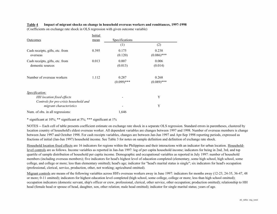
Table 4 Impact of migrant shocks on change in household overseas workers and remittances, 1997-1998(Coefficients on exchange rate shock in OLS regression with given outcome variable)

OutcomesInitial mean Specifications

(1) (2)

Cash receipts, gifts, etc. from 0.395 0.175 0.238 overseas (0.120) (0.086)***

Cash receipts, gifts, etc. from 0.013 0.007 0.006 domestic sources (0.013) (0.014)

Number of overseas workers 1.112 0.287 0.268(0.099)*** (0.089)***

Specification:HH location fixed effects - YControls for pre-crisis household and migrant characteristics - Y

Num. of obs. in all regressions: 1,646

* significant at 10%; ** significant at 5%; *** significant at 1%

NOTES -- Each cell of table presents coefficient estimate on exchange rate shock in a separate OLS regression. Standard errors in parentheses, clustered by location country of household's eldest overseas worker. All dependent variables are changes between 1997 and 1998. Number of overseas members is change between June 1997 and October 1998. For cash receipts variables, changes are between Jan-Jun 1997 and Apr-Sep 1998 reporting periods, expressed as fractions of initial (Jan-Jun 1997) household income. See Table 3 for notes on sample definition and definition of exchange rate shock.

Household location fixed effects are 16 indicators for regions within the Philippines and their interactions with an indicator for urban location. Household-level controls are as follows. Income variables as reported in Jan-Jun 1997: log of per capita household income; indicators for being in 2nd, 3rd, and top quartile of sample distribution of household per capita income. Demographic and occupational variables as reported in July 1997: number of household members (including overseas members); five indicators for head's highest level of education completed (elementary, some high school, high school, some college, and college or more; less than elementary omitted); head's age; indicator for "head's marital status is single"; six indicators for head's occupation (professional, clerical, service, production, other, not working; agricultural omitted).Migrant controls are means of the following variables across HH's overseas workers away in June 1997: indicators for months away (12-23, 24-35, 36-47, 48 or more; 0-11 omitted); indicators for highest education level completed (high school, some college, college or more; less than high school omitted); occupation indicators (domestic servant, ship's officer or crew, professional, clerical, other service, other occupation; production omitted); relationship to HH head (female head or spouse of head, daughter, son, other relation; male head omitted); indicator for single marital status; years of age.

afc_tables mig_remit

Table 5 Impact of migrant shocks on change in household income and expenditures, 1997-1998(Coefficients on exchange rate shock in OLS regression with given outcome variable)

OutcomesInitial mean Specifications

(1) (2)

Total household income 1.000 0.258 0.26(0.162) (0.126)**

Wage and salary income 0.234 0.027 -0.008(0.044) (0.050)

Entrepreneurial income 0.166 0.041 0.029(0.034) (0.041)

Other sources of income 0.6 0.189 0.239(includes remittances) (0.137) (0.100)**

Total household expenditures 1.000 -0.042 -0.048(0.066) (0.069)

Food expenditures 0.452 -0.01 -0.007(0.036) (0.034)

Non-food expenditures 0.548 -0.032 -0.041(0.057) (0.063)

Specification:HH location fixed effects - YControls for pre-crisis household and migrant characteristics - Y

Num. of obs. in all regressions: 1,646

* significant at 10%; ** significant at 5%; *** significant at 1%NOTES -- Each cell of table presents coefficient estimate on exchange rate shock in a separate OLS regression. Standard errors in parentheses, clustered by location country of household's eldest overseas worker. All dependent variables are changes between Jan-Jun 1997 and Apr-Sep 1998 reporting periods. Income changes are expressed as fractions of initial (Jan-Jun 1997) household income. Expenditure changes are expressed as fractions of initial (Jan-Jun 1997) expenditures. See Table 3 for notes on sample construction and variable definitions, and Table 4 for list of control variables.

afc_tables inc_exp

Table 6 Impact of migrant shocks on change in ownership of durable goods, Jan 1998 - Oct 1998(Coefficients on exchange rate shock in OLS regression with given outcome variable)

Outcomes Initial mean Specifications(1) (2)

Radio 0.836 0.04 0.088(0.070) (0.069)

Television 0.828 0.062 0.095(0.035)* (0.035)***

Living room set 0.755 0.039 0.058(0.044) (0.030)*

Dining set 0.677 0.097 0.099(0.076) (0.064)

Refrigerator 0.636 0 -0.01(0.064) (0.058)

Vehicle 0.129 0.168 0.144(0.027)*** (0.039)***

Specification:HH location fixed effects - YControls for pre-crisis household and migrant characteristics - Y

Num. of obs. in all regressions: 1,646

* significant at 10%; ** significant at 5%; *** significant at 1%NOTE -- Each cell of table presents coefficient estimate on exchange rate shock in a separate OLS regression. Standard errors in parentheses, clustered by location country of household's eldest overseas worker. All dependent variables are changes in indicator variables for ownership of given item between Jan 1998 and Oct 1998. See Table 3 for notes on sample construction and variable definitions, and Table 4 for list of control variables.

afc_tables durgoods

Table 7 Impact of migrant shocks on change in household labor supply by worker category, 1997-1998(Coefficients on exchange rate shock in OLS regression with given outcome variable)

Outcomes Initial mean Specifications(1) (2)

Total hours worked 72.6 9.276 5.266(9.934) (8.809)

Hours worked:

For employer outside household 39.6 5.103 0.645(8.100) (8.884)

In self employment 21.5 8.365 9.966(4.468)* (4.744)**

As employer in own family-operated 3.2 1.153 0.829farm or business (1.799) (2.321)

As worker with pay in own family-operated 0.8 -0.126 -0.538farm or business (0.806) (0.735)

As worker without pay in own family-operated 7.6 -5.219 -5.636farm or business (3.464) (3.761)

Specification:HH location fixed effects - YControls for pre-crisis household and migrant characteristics - Y

Num. of obs. in all regressions: 1,646

* significant at 10%; ** significant at 5%; *** significant at 1%NOTE -- Each cell of table presents coefficient estimate on exchange rate shock in a separate OLS regression. Standard errors in parentheses, clustered by location country of household's eldest overseas worker. All dependent variables are changes in hours worked in past week by non-overseas household members, between Jul 1997 and Oct 1998 surveys. See Table 3 for notes on sample construction and variable definitions, and Table 4 for list of control variables.

afc_tables hhwork

Table 8 Impact of migrant shocks on changes in schooling and labor supply of children and young adults, 1997-98(Coefficients on exchange rate shock in OLS regression with given outcome variable)

Panel A: Ages 10-17 Females MalesControl variables included? Control variables included?

OutcomesInitial mean No Yes Initial

mean No Yes

Student indicator 0.95 0.117 0.13 0.93 0.022 0.068(0.086) (0.061)** (0.050) (0.061)

Total hours worked 0.64 -2.753 -2.14 1.53 -1.448 -3.234(2.044) (2.246) (1.711) (1.411)**

Hours worked:

For employer outside household 0.25 -1.276 -0.547 0.43 -0.52 -0.268(1.392) (2.023) (0.978) (1.411)

In self-employment, as employer, or as worker with pay 0.02 0.216 0.243 0.18 1.858 1.976in own family-operated farm or business (0.151) (0.228) (0.639)*** (1.100)*

As worker without pay in own family-operated 0.38 -1.693 -1.837 0.93 -2.786 -4.942farm or business (0.793)** (0.936)* (1.297)** (1.533)***

Num. of obs. in all regs. in column: 579 579 609 609

Panel B: Ages 18-24 Females MalesControl variables included? Control variables included?

OutcomesInitial mean No Yes Initial

mean No Yes

Student indicator 0.43 0.268 0.11 0.37 0.161 0.217(0.238) (0.194) (0.113) (0.121)*

Total hours worked 11.95 3.581 5.353 19.57 1.576 -4.106(8.054) (7.673) (6.312) (6.555)

Hours worked:

For employer outside household 9.30 5.291 5.613 12.02 -3.621 -4.391(8.549) (7.516) (8.194) (7.946)

In self-employment, as employer, or as worker with pay 1.29 -2.824 -0.633 3.84 7.67 8.34in own family-operated farm or business (2.228) (3.657) (6.655) (3.676)**

As worker without pay in own family-operated 1.37 1.115 0.373 3.71 -2.474 -8.055farm or business (1.630) (2.169) (2.947) (3.160)**

Num. of obs. in all regs. in column: 336 336 414 414

* significant at 10%; ** significant at 5%; *** significant at 1%NOTE -- Each cell of table presents coefficient estimate on exchange rate shock in a separate OLS regression. Standard errors in parentheses, clustered by location country of household's eldest overseas worker. Unit of observation is an individual. Individuals are relations of the household head who are not overseas in Jul 1997 (from households with a migrant overseas in June 1997) and who are successfully matched (on the basis of age and gender) with an individual in the same household in Oct 1998. See Data Appendix for details of match process. All dependent variables are changes between Jul 1997 and Oct 1998. "Student indicator" is change in an indicator that student is person's primary occupation (values are -1, 0, or 1). "Hours worked" variables are changes in numbers of hours in respective type of work. Initial means are of levels of respective outcome variables in July 1997.Each regression includes household location fixed effects and controls for individual, household and migrant characteristics. See Table 4 for list of household and migrant control variables. Individual characteristics controls (as reported in July 1997) are: fixed effects for each year of age; gender indicator, indicator for "marital status is single", indicator for "primary activity is student", indicator for "not in labor force", and five indicators for highest schooling level completed (elementary, some high school, high school, some college, and college or more).

afc_tables indiv_1017_1824

Table 9 Impact of migrant shocks on changes in labor supply of adult household members, 1997-1998(Coefficients on exchange rate shock in OLS regression with given outcome variable)

Females MalesControl variables included? Control variables included?

OutcomesInitial mean No Yes Initial

mean No Yes

Total hours worked 20.67 2.969 0.066 35.22 3.708 4.582(4.232) (2.786) (4.376) (3.281)

Hours worked:

For employer outside household 9.02 -1.517 -1.675 17.28 -0.683 -0.508(1.318) (1.427) (3.105) (2.058)

In self-employment 8.55 3.172 1.977 12.87 6.846 8.764(2.980) (1.647) (5.012) (4.876)*

As employer in own family-operated 0.57 -1.303 -1.895 3.06 -0.093 -1.308farm or business (1.005) (1.133)* (2.940) (2.589)

As worker with pay in own family-operated 0.02 -0.162 0.003 0.19 1.251 0.923farm or business (0.148) (0.141) (0.493)** (0.402)**

As worker without pay in own family-operated 2.51 2.779 1.656 1.82 -3.613 -3.289farm or business (2.049) (2.123) (1.809)* (2.117)

Num. of obs. in all regs. in column: 1,360 1,360 926 926

* significant at 10%; ** significant at 5%; *** significant at 1%NOTES -- Each cell of table presents coefficient estimate on exchange rate shock in a separate OLS regression. Household members included in regression if aged 25-64 and are relatives of household head. Standard errors in parentheses, clustered by location country of household's eldest overseas worker. Unit of observation is an individual. See previous table for all other notes.

afc_tables indiv_2564

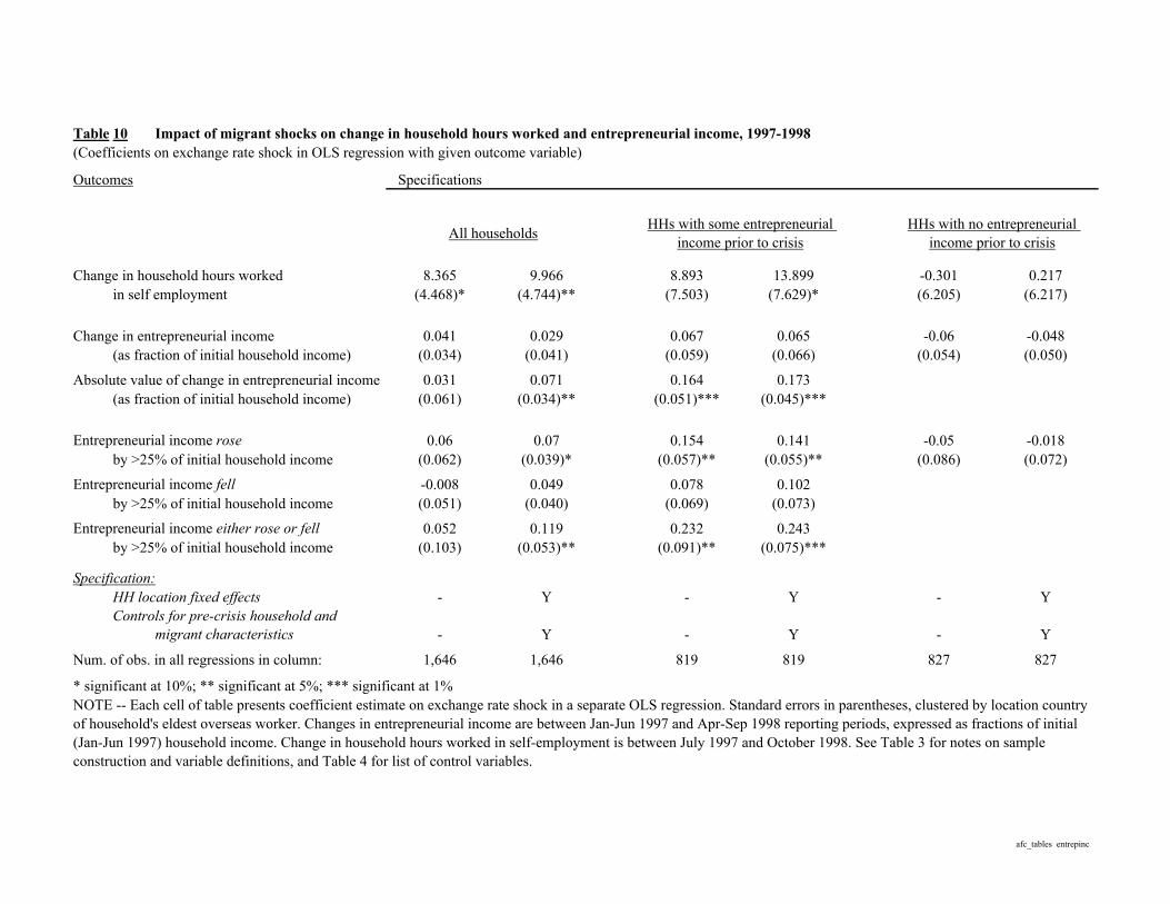
Table 10 Impact of migrant shocks on change in household hours worked and entrepreneurial income, 1997-1998(Coefficients on exchange rate shock in OLS regression with given outcome variable)

Outcomes Specifications

Change in household hours worked 8.365 9.966 8.893 13.899 -0.301 0.217in self employment (4.468)* (4.744)** (7.503) (7.629)* (6.205) (6.217)

Change in entrepreneurial income 0.041 0.029 0.067 0.065 -0.06 -0.048(as fraction of initial household income) (0.034) (0.041) (0.059) (0.066) (0.054) (0.050)

Absolute value of change in entrepreneurial income 0.031 0.071 0.164 0.173(as fraction of initial household income) (0.061) (0.034)** (0.051)*** (0.045)***

Entrepreneurial income rose 0.06 0.07 0.154 0.141 -0.05 -0.018by >25% of initial household income (0.062) (0.039)* (0.057)** (0.055)** (0.086) (0.072)

Entrepreneurial income fell -0.008 0.049 0.078 0.102by >25% of initial household income (0.051) (0.040) (0.069) (0.073)

Entrepreneurial income either rose or fell 0.052 0.119 0.232 0.243by >25% of initial household income (0.103) (0.053)** (0.091)** (0.075)***

Specification:HH location fixed effects - Y - Y - YControls for pre-crisis household and migrant characteristics - Y - Y - Y

Num. of obs. in all regressions in column: 1,646 1,646 819 819 827 827

* significant at 10%; ** significant at 5%; *** significant at 1%NOTE -- Each cell of table presents coefficient estimate on exchange rate shock in a separate OLS regression. Standard errors in parentheses, clustered by location country of household's eldest overseas worker. Changes in entrepreneurial income are between Jan-Jun 1997 and Apr-Sep 1998 reporting periods, expressed as fractions of initial (Jan-Jun 1997) household income. Change in household hours worked in self-employment is between July 1997 and October 1998. See Table 3 for notes on sample construction and variable definitions, and Table 4 for list of control variables.

HHs with no entrepreneurial income prior to crisis

HHs with some entrepreneurial income prior to crisisAll households

afc_tables entrepinc

Table 11 Impact of migrant shocks on change in entrepreneurial income by source, 1997-1998(Households with nonzero pre-crisis entrepreneurial income)

(Coefficients on exchange rate shock in OLS regression with given outcome variable)

Specifications

OutcomesInitial mean

Crop farming and gardening 0.134 -0.029 -0.04 0.069 0.051(0.032) (0.035) (0.053) (0.032)

Wholesale and retail 0.094 0.014 0.012 0.07 0.088(0.032) (0.037) (0.020)*** (0.019)***

Transport, storage, and 0.039 0.063 0.082 0.012 0.007communication services (0.022)*** (0.025)*** (0.016) (0.021)

Community, social, recreational 0.022 -0.015 -0.029 -0.02 -0.022and personal services (0.011) (0.016)* (0.024) (0.030)

Fishing 0.014 0.009 0.008 0.009 0.007(0.012) (0.011) (0.014) (0.009)

Livestock and poultry raising 0.012 0.014 0.023 0.012 0.024(0.011) (0.018) (0.014) (0.016)

Manufacturing 0.012 0.016 0.012 -0.005 -0.004(0.010) (0.013) (0.010) (0.012)

Construction 0.001 -0.008 -0.007 -0.002 -0.001(0.005)* (0.005) (0.005) (0.003)

Forestry and hunting 0.001 0.003 0.002 0.006 0.003(0.006) (0.005) (0.006) (0.004)

Mining and quarrying 0.001 -0.002 -0.001 -0.002 -0.003(0.003) (0.002) (0.002) (0.002)

Other, n.e.c. 0.003 0 0 0.006 0.007(0.002) (0.004) (0.005) (0.005)

Specification:HH location fixed effects - Y - YControls for pre-crisis household and migrant characteristics - Y - Y

Num. of obs. in all regressions: 819

* significant at 10%; ** significant at 5%; *** significant at 1%NOTE -- Each cell of table presents coefficient estimate on exchange rate shock in a separate OLS regression. Standard errors in parentheses, clustered by location country of household's eldest overseas worker. Changes in household income from each entrepreneurial source are between Jan-Jun 1997 and Apr-Sep 1998 reporting periods, expressed as fractions of initial (Jan-Jun 1997) household income. See Table 3 for notes on sample construction and variable definitions, and Table 4 for list of control variables.

Change in entrepreneurial income

Absolute value of change in entrepreneurial income

afc_tables ea_categs

Table 12 Impact of migrant shocks on change in detailed food expenditures, 1997-1998(Coefficients on exchange rate shock in OLS regression with given outcome variable)

Outcomes Initial mean Specifications(1) (2)

Food at home 0.419 -0.009 0.001(0.031) (0.027)

Cereal and cereal preparation 0.136 0.02 0.017(0.006)*** (0.005)***

Meat and meat preparation 0.077 -0.013 -0.007(0.012) (0.011)

Fish and marine products 0.059 -0.014 -0.014(0.006)** (0.007)**

Fruits and vegetables 0.042 -0.007 -0.008(0.005) (0.005)

Dairy products and eggs 0.033 0.001 0.004(0.009) (0.008)

Non-alcoholic beverages 0.015 0.002 0.001(0.003) (0.003)

Coffee, cocoa, tea 0.013 0.006 0.007(0.002)*** (0.002)***

Roots and tubers 0.007 0.000 0.000(0.003) (0.002)

Food, n.e.c. 0.038 -0.004 -0.001(0.006) (0.007)

Food outside the home 0.033 0.000 -0.008(0.010) (0.012)

Regression includes:HH location fixed effects - YControls for pre-crisis household and migrant characteristics - Y

Num. of obs. in all regressions: 1,646

* significant at 10%; ** significant at 5%; *** significant at 1%NOTE -- Each cell of table presents coefficient estimate on exchange rate shock in a separate OLS regression. Standard errors in parentheses, clustered by location country of household's eldest overseas worker. All dependent variables are changes between Jan-Jun 1997 and Apr-Sep 1998 reporting periods, expressed as fractions of initial (Jan-Jun 1997) household expenditures. See Table 3 for notes on sample construction and variable definitions, and Table 4 for list of control variables.

afc_tables food

Table 13 Impact of migrant shocks on change in detailed non-food expenditures, 1997-1998(Coefficients on exchange rate shock in OLS regression with given outcome variable)

Outcomes Initial mean Specifications(1) (2)

Housing services 0.133 -0.04 -0.051(0.027) (0.022)**

Fuel, light, and water 0.056 0.000 -0.002(0.010) (0.010)

Education 0.054 0.016 0.026(0.010) (0.013)**

Transportation and communication 0.049 0.006 0.003(0.009) (0.011)

Personal care and effects 0.040 -0.009 -0.006(0.007) (0.006)

Clothing, footwear, and other wear 0.035 -0.01 -0.007(0.011) (0.013)

Durable furnishing 0.029 -0.005 -0.006(0.018) (0.015)

Special family occasions 0.026 -0.016 -0.016(0.009)* (0.007)**

Medical care 0.022 -0.03 -0.029(0.030) (0.039)

Household operations 0.021 -0.003 -0.001(0.005) (0.007)

Taxes 0.018 0.013 0.008(0.010) (0.009)

House maintenance and repair 0.015 0.002 0.002(0.025) (0.029)

Tobacco 0.010 0.002 0.003(0.005) (0.004)

Gifts and contributions to others 0.007 0.012 0.011(0.005)*** (0.004)**

Alcoholic beverages 0.007 0.002 0.000(0.002) (0.002)

Recreation 0.005 0.004 0.007(0.003) (0.004)

Non-durable furnishing 0.003 0.001 0.001(0.001) (0.001)

Other expenditures 0.019 0.021 0.015(0.029) (0.026)

Regression includes:HH location fixed effects - YControls for pre-crisis household and migrant characteristics - Y

Num. of obs. in all regressions: 1,646

* significant at 10%; ** significant at 5%; *** significant at 1%NOTE -- Each cell of table presents coefficient estimate on exchange rate shock in a separate OLS regression. Standard errors in parentheses, clustered by location country of household's eldest overseas worker. All dependent variables are changes between Jan-Jun 1997 and Apr-Sep 1998 reporting periods, expressed as fractions of initial (Jan-Jun 1997) household consumption. See Table 3 for notes on sample construction and variable definitions, and Table 4 for list of control variables.

afc_tables nfood

Table 14 Impact of migrant shocks by pre-crisis income group, 1997-1998(Coefficients on exchange rate shock in OLS regression with given outcome variable)

Dependent variable:

Change in hours worked

in self-employment

Absolute value of change in

entrepreneurial income

Change in vehicle

ownership

Change in student status (females aged

10-17)

Change in student status

(males aged 10-17)

Change in number of household members overseas

Change in cash receipts from

overseas

Unit of observation, and sample: Households with nonzero

pre-crisis entrepreneurial

income

Households with nonzero

pre-crisis entrepreneurial

income

All households All individuals All individuals All households All households

Coefficient estimates:

(Exchange rate shock)*(Low income) 10.338 0.19 0.022 0.096 0.021 0.127 0.209(14.139) (0.073)*** (0.052) (0.073) (0.129) (0.195) (0.158)

(Exchange rate shock)*(Low-to-middle income) 15.67 0.16 0.259 0.026 0.275 0.405 0.227(9.018)* (0.071)** (0.152)* (0.073) (0.118)** (0.175)** (0.179)

(Exchange rate shock)*(Middle-to-high income) 16.806 0.251 0.223 0.254 0.022 0.39 0.32(9.594)* (0.070)*** (0.066)*** (0.109)** (0.111) (0.111)*** (0.117)***

(Exchange rate shock)*(High income) 14.345 0.034 0.094 0.014 0.006 0.167 0.17(16.412) (0.046) (0.091) (0.103) (0.145) (0.212) (0.172)

Num. of obs.: 819 819 1,646 579 609 1,646 1,646

* significant at 10%; ** significant at 5%; *** significant at 1%NOTE -- Each column of table is a separate OLS regression. Standard errors in parentheses, clustered by location country of household's eldest overseas worker. Changes are between 1997 and 1998, except for vehicle ownership which is change between Jan 1998 and Oct 1998. Change in cash transfers from overseas and in entrepreneurial income expressed as fraction of initial (Jan-Jun 1997) household income. Income groups defined on basis of position in initial (Jan-Jun 1997) distribution of household per capita income in estimation sample. "Low income" households are below 25th percentile, "Low-to-middle-income" households are in 25th-50th percentile, "Middle-to-high income" households are in 50th-75th percentile, and "High-income" households are above 75th percentile. Each regression includes household location fixed effects and controls for household and migrant characteristics (see Table 4 for list of these control variables). Individual-level regressions also include controls for individual-level control variables (see Table 7 for list of these control variables). Each regression also includes main effects of initial income group variables as independent variables.

afc_tables heteffect

Appendix Table 1 Predicting migrant shocks with pre-shock household characteristics(Ordinary least-squares regression results)

Dependent variable: Exchange rate shock Num. of observations 1,646R-squared 0.09

Household per capita income percentile Household head's highest education level Household head's occupation Household size -0.005 (indicators, lowest quartile excluded) (indicators, less than elementary excluded) (indicators, agriculture excluded) (0.003)*

25th-50th 0.032 Elementary 0.022 Professional 0.004(0.020) (0.014) (0.013)

50th-75th 0.008 Some high school 0.024 Clerical -0.001(0.021) (0.021) (0.016)

Above 75th 0.001 High school 0.042 Service -0.014(0.032) (0.018)** (0.025)

Some college 0.048 Production -0.012F-stat: joint signif of these vars.: 3.532 (0.031) (0.013)

P-value: 0.021 College or more 0.053 Other 0.003(0.036) (0.009)

Not working 0.067F-stat: joint signif of these vars.: 2.589 (0.047)

P-value: 0.036F-stat: joint signif of these vars.: 1.033

P-value: 0.414Household location indicators (16 region indicators interacted with urban location indicator)F-stat: joint signif of these vars.: 14.284

P-value: 0.000

Overseas workers' months away Overseas workers' education Overseas workers' occupation Overseas workers' position in household (fraction of HH overseas workers in each category, (fraction of HH overseas workers in each category, (fraction of HH overseas workers in each category, (fraction of HH overseas workers in each cat

less than 12 months excluded) less than high school excluded) production worker excluded) male household head excluded)12-23 months 0.013 High school -0.013 Domestic servant 0.039 Female head or -0.027

(0.008) (0.012) (0.046) spouse of head (0.039)24-35 months 0.036 Some college -0.038 Ship's officer or crew -0.057 Daughter of head -0.012

(0.010)*** (0.022)* (0.050) (0.050)36-47 months 0.041 College or more -0.021 Professional -0.005 Son of head -0.009

(0.015)*** (0.022) (0.043) (0.023)48 months or more 0.043 Clerical 0.05 Other relation -0.001

(0.019)** F-stat: joint signif of these vars.: 2.658 (0.044) (0.029)P-value: 0.057 Other service 0.031

F-stat: joint signif of these vars.: 4.128 (0.029) F-stat: joint signif of these vars.: 0.340P-value: 0.005 Other occupation -0.064 P-value: 0.850

(0.044)

F-stat: joint signif of these vars.: 3.284P-value: 0.008

* significant at 10%; ** significant at 5%; *** significant at 1%NOTE -- All coefficient estimates are from a single OLS regression. Standard errors in parentheses, clustered by location country of household's eldest overseas worker. Dependent variable is household-specific exchange rate shock. Income variables are as of Jan-Jun 1997. Head's characteristics and household size are as of July 1997. Household size includes overseas members. Overseas workers' characteristics are for those away in June 1997 (reported in Oct 1997). Coefficients on household location indicators not reported. See Table 3 for definition of exchange rate shock and definition of sample households.

afc_tables predshock

Appendix Table 2 Impact of migrant shocks on attrition from household and individual panels, Jul 1997- Oct 1998(Coefficients on exchange rate shock in OLS regression)

A: HouseholdsMean of outcome

Coef. on shock

Outcome: attrition indicator 0.056 0.008(0.032)

Number of obs. 1,743

B: Individual Males Ages 10-17 Ages 18-24 Ages 25-64Mean of outcome

Coef. on shock

Mean of outcome

Coef. on shock

Mean of outcome

Coef. on shock

Outcome: attrition indicator 0.238 -0.091 0.286 -0.051 0.235 0.081(0.102) (0.092) (0.096)

Number of obs. 800 581 1,210

C: Individual Females Ages 10-17 Ages 18-24 Ages 25-64Mean of outcome

Coef. on shock

Mean of outcome

Coef. on shock

Mean of outcome

Coef. on shock

Outcome: attrition indicator 0.23 0.018 0.35 0.021 0.213 0.008(0.111) (0.077) (0.067)

Number of obs. 752 518 1,729

* significant at 10%; ** significant at 5%; *** significant at 1%

Each regression includes household location fixed effects and controls for household and overseas worker characteristics. Individual-level regressions also include control variables for the following individual characteristics (as reported in July 1997): gender indicator, indicator for single marital status, indicator for "primary activity is student", indicator for "not in labor force", and five indicators for highest schooling level completed (elementary, some high school, high school, some college, and college or more). See Table 4 for list of household and migrant control variables.

NOTE -- Each cell of table presents coefficient estimate on exchange rate shock in a separate OLS regression. Standard errors in parentheses, clustered by location country of household's eldest overseas worker. Unit of observation is the household in Part A, and the individual in Parts B and C. Individuals are those observed in Jul 1997 (from households with a migrant overseas in June 1997). For households, attrition indicator equal to 1 if household was excluded from sample because it changed dwellings between July 1997 and October 1998, or had missing data on outcome variables in October 1998. For individuals, attrition indicator equal to 1 if individual is not successfully matched (on the basis of age and gender) with an individual in the same household in Oct 1998, and 0 otherwise (see Data Appendix for details of match process).

afc_tables indiv_attrit

Figures 1A - 1D: Impact of exchange rate shocks on household outcomes

Figure 1A: Change in cash receipts from overseas Figure 1B: Change in educational expenditures

Figure 1C: Change in hours worked in self-employment Figure 1D: Absolute value of change in entrepreneurial income(only HHs with nonzero pre-crisis entrepreneurial income) (only HHs with nonzero pre-crisis entrepreneurial income)

NOTE-- Change is between Jul 1997 and Oct 1998.

Note for all figures-- Black dot is mean change in an outcome for households with given exchange rate shock. Dashed vertical lines indicate 95% confidence intervals (standard errors clustered by overseas location of household's eldest overseas worker). See Table 3 for definition of exchange rate shock and definition of sample households.

NOTE-- Change is between Jan-Jun 1997 and Apr-Sep 1998, expressed as share of pre-crisis total HH income.

NOTE-- Change is between Jan-Jun 1997 and Apr-Sep 1998, expressed as share of pre-crisis total HH expenditures.

NOTE-- Change is between Jan-Jun 1997 and Apr-Sep 1998, expressed as share of pre-crisis total HH income.

0.01

0.012

0.014

0.016

0.018

0.02

0.022

0.024

0.026

0.028

0.03

E.R. shock < 0.35 E.R. shock > 0.35

Cha

nge

in e

duca

tiona

l exp

endi

ture

s

-16

-14

-12

-10

-8

-6

-4

-2

0

E.R. shock < 0.35 E.R. shock > 0.35

Cha

nge

in H

H h

ours

wor

ked

in se

lf-em

ploy

men

t

0.2

0.21

0.22

0.23

0.24

0.25

0.26

0.27

0.28

0.29

0.3

E.R. shock < 0.35 E.R. shock > 0.35

Abs

olut

e va

lue

of c

hang

e in

ent

repr

eneu

rial i

ncom

e

0.05

0.07

0.09

0.11

0.13

0.15

0.17

0.19

0.21

0.23

0.25

E.R. shock < 0.35 E.R. shock > 0.35

Cha

nge

in c

ash

trans

fers

from

ove

rsea

s

Figures 2A and 2B: Household investment decision

2A: Overseas income and utility gain from investment in entrepreneurial activity

2B: Overseas income and entrepreneurial labor supply

NOTES -- Graphs are solution to household entrepreneurial investment problem in Section 2 of text, as overseas income (R ) changes, where utility from consumption (x i ) and leisure (li ) in period i is given by (x i ) α + γ li . Parameter values are: T =24, α =.5, p =0.5, v =20, u =6, γ =0.5, C =5, A =1.5. Range of overseas income depicted in both figures is [1.0,20.0].

Risk-free entrepreneurship (Q* )Risky entrepreneurship (Q** )

Overseas income

Util

ity g

ain

from

inve

stm

ent

Overseas income

Entr

epre

neur

ial l

abor

sup

ply

0.7

0.8

0.9

1

1.1

1.2

1.3

1.4

1.5

1.6

1.7Ju

l96

Aug

96

Sep9

6

Oct

96

Nov

96

Dec

96

Jan9

7

Feb9

7

Mar

97

Apr

97

May

97

Jun9

7

Jul9

7

Aug

97

Sep9

7

Oct

97

Nov

97

Dec

97

Jan9

8

Feb9

8

Mar

98

Apr

98

May

98

Jun9

8

Jul9

8

Aug

98

Sep9

8

Oct

98

Month

NOTES-- Exchange rates are as of last day of each month. Data source is Bloomberg L.P.

Figure 3: Exchange Rates in Selected Locations of Overseas Filipinos, July 1996 to October 1998(Philippine pesos per unit of foreign currency, normalized to 1 in July 1996)

Malaysia

Korea

Taiwan

Saudi Arabia, Hong Kong, U.S., U.A.E., Qatar

Singapore

Japan

Start of Asian financial crisis

(July 1997)

Phili

ppin

e pe

sos p

er u

nit o

f for

eign

cur

renc

y (J

uly

1996

= 1

)