International Journal of Social Science and Public Policy

22

©Center for Promoting Education and Research (CPER) USA www.cpernet.org

VOL: 1, ISSUE: 1 January/2019

https://ijssppnet.com/

E-ISSN: xxxx-xxxx

International Journal of Social Science and Public Policy (IJSSPP)

The moderating effect of personal characteristics on service quality and customer satisfaction in Commercial

banks in Rwanda

Philippe Ndikubwimana1

Jean Claude Ndibwirende1

Eugene Muvunyi1

Jean Bosco Ndikubwimana2

College of Business and Economics School of Business

University of Rwanda1& 2 e-mail: [email protected]

Abstract

This study examines the moderating effect of personal characteristics on service quality and customer

satisfaction in commercial banks in Rwanda. The objectives of this study are: to determine the level at which

service quality dimensions affect customer satisfaction in commercial banks in Rwanda; to find out the extent

to which personal characteristics affect the relationship between service quality and customer satisfaction in

commercial banks in Rwanda. Descriptive survey and exploratory design were used. Cluster sampling was

used during data collection. All respondents were selected using convenience sampling technique. The

SERVQUAL questionnaire has been adapted to the Rwandan context to collect data from 384 respondents.

Statements on the dimensions of service quality and customer satisfaction were measured using a 7- point

Likert scale. To achieve objectives of this study and answer research questions, descriptive and inferential

statistics were used. The findings showed that all the service quality dimensions were good predictors of

customer satisfaction. Using the ordered logistic model, it has been shown first that ‘Quality Service’ as a

predictor variable, has an effect on ‘Customer Satisfaction’. It has also been established that most of the

coefficient estimates were individually statistically significant with p< 0.05. Investigating the perceptions of

Rwandan banking customers regarding service quality and satisfaction has indicated positive perceptions, but

continuing to ensure these positive perceptions is important for the continued satisfaction of existing

customers while also providing satisfaction to new customers. From the analysis carried out, it was found out

that the overall service quality perceived by the customers was not satisfactory, as expectations were

higher than perceptions. The findings showed that ‘Marital Status’ had the most weight than all other

variables under Personal Aspect.

Keywords: Service quality, Service quality gaps, Service quality dimensions, Customers’ expectations, Customer

satisfaction

Introduction The need to reinforce service delivery has assumed great significance in recent periods. According to

RDB (2013), the Government of Rwanda is faced with problems of poor customer satisfaction both in public and private sectors that is impeding its progress towards becoming a middle income country by 2020. In this respect, the Rwanda Development Board has been established to improve customer service delivery across all sectors in the economy. Due to increased competition in banking sector particularly in Eastern Africa, Banking industry in Rwanda, has put in place infrastructure, established departments for Customer Service to address the

http://www.cpernet.org/


23




E-ISSN: xxxx-xxxx


needs of their customers. It is not clear if such measures amongst others have helped to improve satisfaction of the bank customer and their retention rates with the respective banks. The main objective of this research is to determine the extent to which personal characteristics moderate the relationship between service quality and customer satisfaction. Specifically include: To determine the level at which age factor affects customer satisfaction in commercial banks in Rwanda. To establish the effect gender on the relationship between service quality and customer satisfaction in commercial banks in Rwanda. To find out the extent to which marital statusaffects the relationship between service quality and customer satisfaction in commercial banks in Rwanda. To establish the effect of level of education on customer satisfaction in commercial banks in Rwanda. Researcher hypothesis include: Personal attitudes significantly moderate the relationship between service quality and customer satisfaction in Commercial banks in Rwanda

Literature review

Personal attitudes and customer satisfaction. A personal attitude is the degree to which an individual holds a favorable or unfavorable judgment of the performance in question (Kamau, 2012). It impacts on customer satisfaction and behavioral outcomes (Laforet and Li, 2005). Consequently, it includes not only effective, but also evaluative considerations. Personal attitude is subject to change and therefore, customer satisfaction may be affected by an individual’s perception, beliefs, attitudes, and values influence his or her experience and involvement with banks’ services. It can be also influenced by educators and practitioners.

Customers tend to be more involved with services or products that they believe can fill their own needs and wants which in return are impacting on their satisfaction. Individual factors like gender, age, education, income level or social class, customer’s personality influence customer’s perception and satisfaction. A consumer does not buy the same products or services at 25 or 65 years. His or her lifestyle, values, environment, activities, hobbies and consumer habits evolve throughout his life. The decision to become a customer of one bank not of another is influenced by characteristics of each customer. The studies done by Jabnoun & Khalifa (2005), confirmed that the need to have banks (Islamic bank, Goshen bank...) that are in line with the society, belief and religion values of the customer especially for women.

In the research done by Bryant & Cha (1996) on four hundred companies using the ACSI, established that there is significant relationship and reliable differences in the levels of satisfaction related to personal factors. This has been confirmed by study by Palvia and Palvia (1999) where they have found that the factor age affects significantly on customer satisfaction through IT. In airline sector, Oyewole (2001) conducted a study on customer satisfaction and stated that educational background, profession, marital status and gender significantly affect customer satisfaction, and however, income and age aspects had no significant influence.

According to Ogden & Ogden (2005) the most important personal characteristics information is marital status because it shows if customers are buying for themselves, for a spouse, or a family with children. Education level is important demographic information because as customers become more educated they demand different products and different levels of service (Kent & Omar, 2003). Kotler& Armstrong (2010) suggest there has been an increase in educated people in the United States and this leads to an increase in the demand for quality products.

A study by Kim & Jin (2002), looked at the number of visits the customers made to their preferred discount shop in Korea and USA, but there were no further analyses made to find any correlations between the number of visits and the different dimensions. Income has a relationship with purchasing decisions, thus high income customers gather information prior to buying a product and this may have an influence on satisfaction (Homburg &Giering, 2001). This study analyzed the effect of demographic factors and education on customer satisfaction.



24




E-ISSN: xxxx-xxxx


Results and Discussion

In this study, customer satisfaction is a function of service quality dimensions (TAN, REL, RES, ASS, and EMP) moderated by Personal Attitudes (PA). To estimate the effect or impact on probability the probabilities for each category when all independent values are set to their mean values by changing values we used predicted probabilities by using p-value. A positive coefficient indicates an increased chance that a subject with a higher score on the independent variable will be observed in a higher category. A negative coefficient indicates that the chances that a subject with a higher scores on the independent variable will be observed in a lower category. This is a maximum likelihood estimator, not a least squares estimator. The various parameters are present in the likelihood function. Let X denote the predictors of the model and Y be the response variable. In this case X defines all independent variables under investigation, (that is RELi, ASSi, TANi, EMPi, RESi, SVi, PAi, TAi, i =1,…,4 or 5 see appendix 2 ) as defined in the previous section and Y (Customer Satisfaction, that is CSi, i =1,…,5 ) is the dependent variable. To define the cumulative log its quantities, let

1,,1,

1loglog

Jj

XF

XFXFitXL

j

j

jj ……………………………………… (1)

Where XjYPXFj | the cumulative probability for response category j, and J is the total number of response

categories (that is Y takes on values J,,1 ). This model is known as the proportional-odds model because the odds

ratio of the event is independent of the category j. The odds ratio is assumed to be constant for all categories.

Thus, XL j are then the log-odds of jY against jY ? In practice, the proportion odds model is represented by

1,,1,11 JjXXXL kkjj …………………………………………… (2)

Where jj , , 𝛽𝑘 are parameters to be estimated? Observe that positive l is normally associated with increasing

odds of being less than a given value j with increasing lX . What this implies is that a positive coefficient leads to

increase in probability of being in lower numbered categories with increase in lX while holding all other variables

constant.

Testing the effect of ‘Service Quality’ on ‘Customer satisfaction’ Case 1:

For this test, the model (2) is used where then XL j stands for the response variable and

11111 ,,,, RESEMPTANASSRELX . Variables used are clearly defined (labeled) (see appendix 1&2). Table 1.1

contains the output when in the model (2), the response variable, 1CSXL j , where ‘CS1 = I am satisfied about the

use of banking services’. The LR chi2(5) = 166.27 where 5 in parenthesis indicates the number of predictors in the model; Likelihood (LR) ratio Chi-square test that at least one of the predictors' regression coefficient is not equal to zero in the model. The higher is LR, the higher is the likelihood of rejecting the null hypothesis with higher statistical significant measure. It can be observed that P-value= 0.0000 which is far less that α = 0.05, level of significance. This leads to rejection of the null hypothesis, H0 in favor of the alternative hypothesis, Ha. Hence, the independent variables considered in this case have an impact on the dependent variable, CS1.

In addition, this impact is quite significant, since all of P-value are zeros (see column 5, Table 1.1). This defines the probability that a particular z test statistic is as extreme as, or more so, than what has been observed under the null hypothesis. P = 0.000 everywhere suggests that the regression coefficients have been found to be statistically



25




E-ISSN: xxxx-xxxx


significant for each independent variable used. That means that they are certainly different from zeros in estimating the response, CS1 given all the independent variables, 11111 ,,,, RESEMPTANASSRELX . This can also be

observed for each [95% Conf. Interval] above which does not contain zero, implying none of the regression coefficients in the model is zero.

The column 2 of Table 1 contains the estimated coefficient scores for each predictor. This depicts the ordered log-odds estimate for a unit increase in one of the X variables score on the expected CS1level given the other variables are held constant in the model. A positive coefficient indicates an increased chance that a subject with a higher score on the independent variable will be observed in a higher category. A negative coefficient indicates that the chances that a subject with a higher scores on the independent variable will be observed in a lower category. For instance, it can be observed that a change of one unit in REL1 test score would result in increase of 0.2407 in the ordered log-odds of being in a higher CS1 category while all the other variables in the model are held constant. Similar interpretation can be made for RES1, ASS1 which, for a unit change would result respectively in a 0.186866, and 0.2533398 increase in the ordered log-odds of being in a higher CS1 category while all the other variables in the model are held constant.

Even though the values of P-value are also 0.000 for TAN1 and EMP1 in table 1, their coefficients are all less than zero. This implies that a unit change in TAN1 and EMP1 would result respectively in a 0.2825629 and 0.1412919 decrease in the ordered log-odds of being in a higher CS2 categories while all the other variables in the model are held constant.

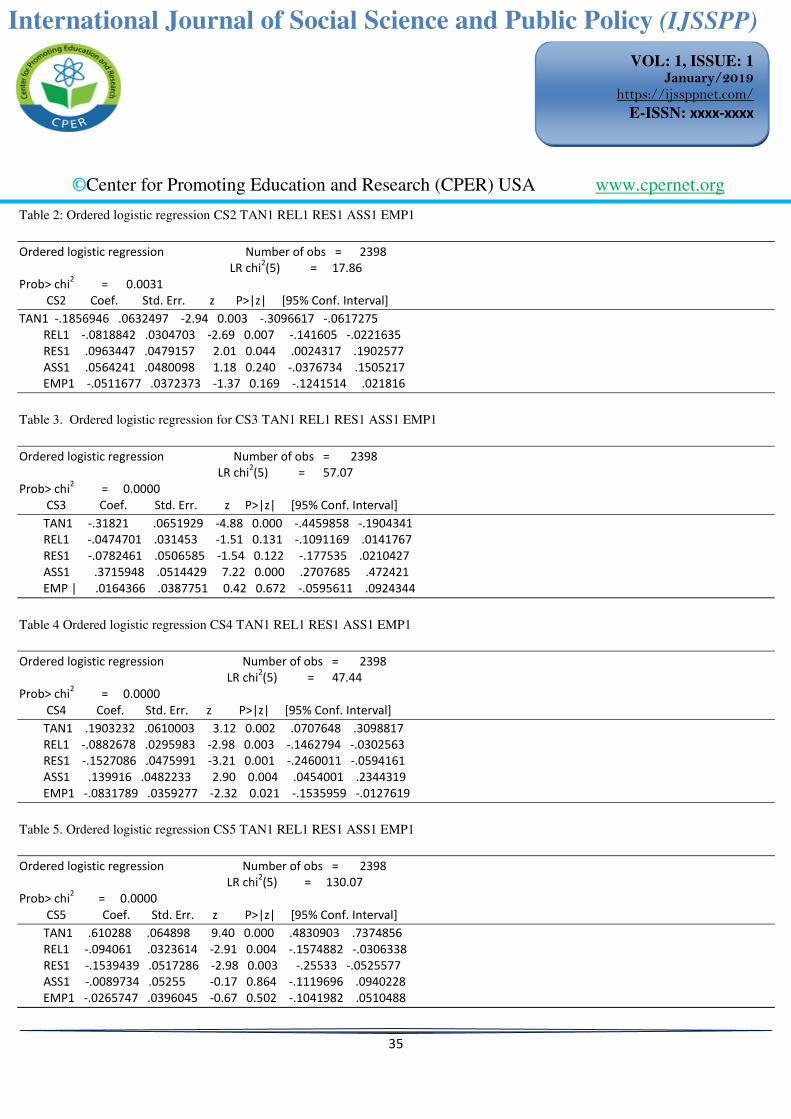
Keeping all the predictors unchanged, table 2 contains results of the investigation when the response variable is CS2, where CS2 stands for ‘Bank does not cost too much’. It is observed that likelihood = 17.86 is not large, and so some coefficient estimates can be expected not to be statistically significant. For instance, the coefficient estimates for ASS1 and EMP1, which are .0564241 -.0511677 are not statistically significant. This implies that the [95% Conf. Interval] indicating the possible values of the null hypothesis do contain indeed zero. The predictors whose coefficients are statistically significant are the ones with the value of p< 0.05. These include the coefficients for TAN1, REL1 and RES1 respectively. However, p = 0.0031 < 0.05 for the entire model.

This result leads to rejection of the H0 in favor of the alternative hypothesis, Ha at 0.05 level of significance. It can be noticed that a unit change in TAN1, REL1 test score would respectively result in a 0.1856946 and 0.0818842 decreases in the odds-ratio of being in the higher CS2 category, while all the other variables in the model are held constant. Also a unit change in RES1 test scores would result in increase of 0.0963447 in the odds-ratio of being in the higher CS2 category, while all the other variables in the model are held constant.

However, the coefficients associated with the predictors ASS1 and EMP1 have been found not to be statistically significant. Keeping all the predictors unchanged as in previous section, table 3 contains results of the investigation when the response variable is CS3, where CS3 stands for ‘Internet connection is always available’. From now onward, we drop comments on the values of likelihood and elaborate on the values of p-value, Coefficient and the interval [95% Conf. Interval]. It is observed that P-value = 0.000 which is less than 0.05. This leads to rejection of H0 in favor of the Ha, at 0.05 level of significance. This implies that that at least one of the coefficients of the predictors is not zero.

How significant are coefficients of the predictors of the regression equation used? Since P< 0.05 for TAN1 and ASS1, their coefficient estimates are statistically significant. A unit change in the TAN1 and ASS1 test scores would result respectively in a 0.31821 and 0.3715948 decrease and increase in the odds-ratio of being in the



26




E-ISSN: xxxx-xxxx


higherCS3category, while all the other variables in the model are held constant. This is confirmed by their [95% Conf. Interval] which do not contain zeros. Other coefficient estimates are found to be not statistically significant.

In table 4, we consider CS4 to be the response variable and observe the following results. P-value = 0.0000< 0.05, in which case we reject the null hypothesis and conclude that the predictors have an impact in the response variable. This is, in fact, statistically significant, since p-values for all predictors are less than 0.05, the level of significance considered. This can be spotted on the individual [95% Conf. Interval] who does not contain zero.

Observe that a unit change in TAN1 and ASS1 test scores would result respectively in 0.1903232 and 0.139916 increases in the odds-ratio of the higher CS4category, while all the other variables in the model are held constant. However, keeping all other variables in the model constant, we observe also that a unit change in REL1, RES1 and EMP1 test scores would result respectively in 0.0882678, 0.1527086 and 0.0831789 decrease in the log-odds of being in the higher CS4 category. This result is not surprising since, taken together REL1, RES1 and EMP1 are all subject to personal appreciation which is somehow difficult to measure. However, the coefficient estimates are statistically significant, since their individual P < 0.05, the level of significance used.

Table 5 contains output where is considered a response variable and all other predictors used previously remain unchanged. It can noticed that p-value = 0.0000, and this is less than 0.05 and so the null hypothesis is rejected in favor of the alternative one, at 0.05 level of significance. The coefficients estimates of the predictors are all statistically significant, since P < 0.05, except for the predictors ASS1 and EMP1.

Observe that a unit change in of TAN1, REL1 and RES1 test scores would result respectively in .610288 increases, 0.094061 and 0.1539439 decrease in the log-odds of being in the higher CS5 categories, while all other variables are held constant. Similarly a unit change in ASS1 and EMP1 test scores result respectively in 0.0089734 and 0.0265747 decreases in the log-odds of being in the higher CS5 categories, while all other variables are kept constant. In case one that we have just discussed, an α= 0.001 as level of significance could have worked as well, since most of the value P were far less than 0.05. This indicates strong results as to the significance of the coefficient estimates of the model used.

Case two:

Using the model in (2) for same XL j but 22222 ,,,, RESEMPTANASSRELX , we have the following results.

Table 6 contains the result when CS1 is considered as the response variable. Since p-value= 0.0000, the null hypothesis is rejected in favor of the alternative at 0.05 level of significance. This confirms that, indeed, the predictors have an impact on the response variable. This impact is statistically significant for predictors whose [95% Conf. Interval] do not contain zero, except for TAN2 ‘Bank uses state of the art technology and equipment in their

service’ whose P-value is greater than 0.05.

From the coefficient estimates, it can be observed that a unit change in REL2, RES2, ASS2 and EMP2 predictors test scores results respectively in a 0.3642064 increases, 0.232391 decreases, 0.0978277 increases and 0.0720662 decreases in the log-odds of being in the higher CS1 categories, while all other variables are kept constant. Also a unit change in TAN2 would result in a 0.022519 decreases in the log-odds of being in the higher CS1 categories, while all other variables are kept constant. When we look at the labels of variables where a decrease in the log-odds have been observed, that is ‘TAN2=Bank uses state of the art technology and equipment in their service, RES2= Bank's employees give me prompt service, EMP2= Bank has my best interest at heart’, it is quite possible that this effect is attributable to the use of the expression (or wording) ‘state of the art, prompt, best ’ which are subject to individual perception.



27




E-ISSN: xxxx-xxxx


In table 7, we consider the case when CS2 is the response variable while keeping all other predictors the same. We observe that p-value= 0.0000 and it is less than 0.05, the α level of significance. This result leads to rejection of the null hypothesis. We thus conclude that, at 0.05 level of significance, not all coefficients in the model are all zero. Besides, all the coefficient estimates for all predictors are significant, except for TAN2, whose P-value is greater than 0.05, and of which the [95% Conf. Interval] contains zero. For the remaining predictors, we observe that a unit change in REL2, RES2, ASS2 and EMP2 test scores would result respectively in a 0.1571805 increases, 0.238126 decreases, 0.0979642 and 0.1323964 increases in the log-odds of being in the higher CS2 categories, while all other variables are kept constant. However, a unit change in TAN2 test scores would result in a 0.0801647 decrease in the log-odds of being in the higher CS2, keeping all other variables constant. This could be attributable to the fact that, in the predictor TAN2, the word ‘State of the art’ of which the understanding is subject to customer’s perception, was use in the questionnaire.

In table 8, CS3 has been used as the response variable, keeping other predictors unchanged. It can be observed that p-value = 0.0000 and this coefficient is less than 0.05, the level of significance and so we reject outright the null hypothesis in favor of the alternative one. The coefficient estimates for all predictors are statistically significant, that is their p-value is less than 0.05, except for REL2 and EMP2 whose P is greater than 0.05. As consequence, the respective [95% Conf. Interval] of the latter contain a zero. On the one hand, we observe that a unit change in TAN2, RES2 and ASS2 test scores would result in a 0.232323 units increases, 0.193523 unit decreases and 0.2140068 units increases in the log-odds of being in the higher CS3, keeping all other variables constant.

This increase or decrease is with higher statistical significance since the respective [95% Conf. Interval] does not contain zero, a tested value for the coefficient estimates in the alternative hypothesis. On the other hand, a unit change in REL2 and EMP2 test scores would results in a 0.1151198 and 0.0690596 increase in the log-odds of being in the higher CS3 categories, keeping all other variables constant, but this is very little statistical significance. In table 9, we consider CS4 as the response variable, keeping all other predictors the same. It can be observed that the value of p-value = 0.0000 which is less 0.05, and leads to reject the null hypothesis on favor of the alternative. The coefficient estimates of all predictors are statistically significant except for TAN2 and RES2 whose P-value is greater than 0.05. Eventually, this implies that, with little statistical significance, a unit change in TAN2 and RES2 test scores would result in a 0.0066976 units increase and 0.0779435 units decrease in the log-odds of being in the higher CS4 categories, while we keep all other variables constant. For the remaining predictors, a unit change in each one test score would result in a statistically significant, units increase or decrease in the log-odds of being in the higher CS4 categories, depending on the sign of the coefficient estimate.

In table 10, CS5 is considered as the response variable while all other predictors are same as in section. It can be observed that p-value = 0.0000 and it is less than 0.05, the level of significance. As in previous section, this prompts to reject the null hypothesis in favor of the alternative, at 0.05 level of significance. The coefficient estimates for all predictors are all statistically significant, but for the predictor, TAN2, of which P-value is greater than 0.05.

The interpretation of the magnitude of the coefficient estimates for each predictor follows the same scheme of units increase or units decrease in the log-odds of being in their higher CS5 categories, while keeping all other variables constant. Note that their respective [95% Conf. Interval] does not contain zero at all.

Case 3:

Using the model in (2) for same XL j but 33333 ,,,, RESEMPTANASSRELX

We have the following results: in table 11, CS1 is treated as the response variable and X component the predictors.



28




E-ISSN: xxxx-xxxx


It can be observed that p-value is 0.0164 which is less than 0.05, the level of significance. At this level, the coefficient estimates of the predictors are found not to be statistically significant since their respective p-values are greater than 0.05, except for the predictor ASS3 whose p-value is 0.025. When we look at the nature of both response and predictors variables, this rather low performance could be associated with a mismatch of both variables. On the one hand, CS1 stands for ‘I am satisfied about the use of electronic banking services’.

On the other hand, all the predictors used in this instance deal with the bank’s employees and their service. Precisely, ‘TAN3: The employees are well dressed and neat in appearance, REL3: Bank delivers it services promptly, RES3: Bank's employees are never too busy to respond to my request, ASS3: Bank’s employees are consistently

courteous with me and EMP3: Bank’s employees understand my specific needs.’ These variables have nothing to do with electronic banking service offered by the bank.

These results are quite strong since we still reject the null hypothesis in favor of the alternative one at approximately 0.0164 < 0.05 level of significance. The reading of the coefficient estimates of each predictor follow same scheme as presented earlier. Depending on the sign of this coefficient estimate, a unit change in the predictor test scores would create units increase or decrease in the log-odds of being in the higher CS1 categories, while keeping all other variables constant.

In table 12, CS2 is considered as the response variable while all other predictors used in this case remains unchanged. We observed that p-value = 0.0000, which is less than 0.05, the level of significance. Except for ASS3 and EMP3, at this level, the coefficient estimates of other predictors are found not to be statistically significant, since their respective p-values are greater than 0.05.Again, even though the null hypothesis is rejected, a relative low level performance is attributable once more to a mismatch in the choice of variables in the model. On the one hand, we consider the cost of the bank not being too much as indicator of customer satisfaction and on the other hand, the predictors, TAN3 REL3 RES3 ASS3 EMP3variables as labeled in the preceding section. These seem to be far apart, and this has cause a low level of statistical significance on the coefficient estimates. Otherwise, depending of the sign of the coefficient estimates of each predictor, their reading follow the same scheme of units increase or decrease in the log-odds of being in the higher CS2 categories, while keeping all other variables constant.

In table 13, CS3, labeled ‘Internet connection is always available’ is taken to by the response variable while all other predictors used in this case remain unchanged.

We observed that p-value = 0.0000 and it is less than 0.05, the level of significance. Except for REL3, at this level, all other coefficient estimates of other predictors are found to be statistically significant, since their respective P-values are less than 0.05 and, their individual [95% Conf. Interval] does not contain zero. This suggests outright rejection of the null hypothesis in favor of the alternative.

Once more, depending of the sign of the coefficient estimates of each predictor, their interpretation will follow the same scheme of units increase or decrease in the log-odds of being in the higher CS3 categories, while keeping all other variables constant. For instance, a unit change in REL3 test scores would result in a 0.0433057 increase in the log-odds of being in the higher CS3 categories, while keeping all other variables constant. The same interpretation can be done for the remaining of the predictors.

In table 14, CS4, labeled ‘I feel delighted by the bank's service’ is considered as the response variable while all other predictors used in this case remain unchanged. We observed that p-value = 0.0000 which is less than 0.05, the level of significance, prompting to reject outright the null hypothesis in favor of the alternative. The coefficient estimates of TAN3, REL3 and RES3 are all statistically significant while for the remaining predictors are found not to be statistically significant. The [95% Conf. Interval] of the latter contain zero.



29




E-ISSN: xxxx-xxxx


Clearly, depending on the sign for each coefficient estimate, a unit change in the predictor test scores in this case would result in unit increase or decrease in the log-odds of being in the higher CS4 categories (6 or 7), as depicted in the tab below, while keeping all other variables constant.

For instance, we observe that a unit change in TAN3 test scores would result in a 0.259494 units increase in the log-odds of being the higher CS4 categories (6 or 7), while keeping all other variables constant. All other coefficient estimates follows same pattern of interpretation.

In table 15, CS5, labeled ‘Bank has the variety of services’ is treated as the response variable while all other predictors used in this case remain same. We observed that p-value = 0.0000 which is less than 0.05, the level of significance. This suggests outright rejection of the null hypothesis in favor of the alternative. The coefficient estimates for all predictors are statistically significant, since their individual value of p-value is less than 0.05, level of significance.

Obviously, depending of the sign of each coefficient estimate for each predictor, a unit change in each one of the predictors’ test scores would result in units increase or decrease in the log-odds of being in the higher CS5 categories, as shown in the tab 17 while keeping all other variables constant. For example, a unit change in EMP3 test scores would result in a 0.4182209 increase in the log-odds of being in the higher CS5 categories (6 or 7), while all other variables remain constant.

Case 4:

Using the model in (2) for same XL j but 44444 ,,,, RESEMPTANASSRELX ,

We have the following results: in table 16, CS1, labeled ‘I am satisfied about the use of electronic banking

services’ is treated as the response variable while all component of X, the predictors used in the model. We observed that p = 0.0000 which is less than 0.05, the level of significance. It can be observed that the coefficient estimates of all the predictors used are all statistically significant, except for TAN4, predictor, whose P-value is greater than 0.05. The interpretation of the coefficient estimates for each predictor will follow same scheme as presented in previous cases.

In that line, it can be observed for instance that a unit change in TAN4 test scores would result in a 0.0325614 increase in the log-odds of being in the higher CS1 categories (6 or 7), while keeping all other variable constant. In table 17, CS2, labeled ‘Bank does not cost too much.’ is considered as the response variable while all component of X, the predictors as used in previous section. We observed that p-value = 0.0000 < 0.05, the level of significance. This suggests rejecting the null hypothesis in favor of the alternative one. Thus, clearly the predictors considered in this case have an impact on the response variable.

[

The coefficient estimates for ASS4 and EMP4 predictors are statistically significant at 0.01 level of significance, except for the predictorsTAN4, REL4 and RES4, whose P is greater than 0.005. To interpret the magnitude of these estimates, note that a unit change in RES4, REL4 test scores, for instance, would result in a 0.2326408; .0797363 increase in the log-odds of being in the higher CS2 (6 or 7) respectively, as depicted this tab, while keeping all other variables constant. The same interpretation can be done for remaining coefficient estimates. In table 18, CS3, labeled ‘Internet connection is always available.’ will be considered as the response variable while all component of X, the predictors remain the same. We observed in this case that p-value = 0.0000 and it is less than 0.05, the level of significance. This suggests rejecting the null hypothesis in favor of the alternative hypothesis at 0.05 level of significance.



30




E-ISSN: xxxx-xxxx


The coefficient estimates of the predictors are statistically significant, except for REL4 and RES4 respectively scoring p-value> 0.05. As it stands in Table 19, column 2, depending on the sign of the coefficient, a unit change in the predictors used would result in units increase or decrease in the log-odds of being in the higher CS3 categories (6 or 7) as shown in the tab CS3 below, while keeping all other variables constant.

For instance, a unit change in ASS4 and REL4 test scores would result respectively in 0.1099028 increase and 0.0319669 decrease in the log-odds of being in the higher CS3 categories (6 or 7), while keeping all other variables constant. The same interpretation can be applied to the remaining of the coefficient estimates.

In table 19, CS4, labeled ‘I feel delighted by the bank's service’ will be treated as the response variable while all components of X, the predictors, remain the same. It can be observed in this case also that p-value = 0.0000 which is less than 0.05, the level of significance. Hence, the null hypothesis is rejected in favor of the alternative. We must observe that the coefficient estimates for all predictors are statistically significant, with individual score of p-value = 0.000 As the results stand in column 2, it is quite clear that a unit change in TAN4, REL4, RES4, ASS4 and EMP4 predictors would result respectively in unit increase or decrease, depending on the sign of the coefficient, in the log-odds of being in the higher CS4 categories (6 or 7), while keeping all variables constants.

In table 20, CS5, labeled ‘Bank has the variety of services’ will be treated as the response variable keeping all components of X, the predictors, the same as in the previous section. It is observed that p = 0.0000 which is less than 0.05, the level of significance. The null hypothesis is rejected in this case in favor of the alternative. There is indeed a strong relationship which is statistically significant between the CS5 and all the predictors considered. We observe also that all the coefficient estimates for all predictors are statistically significant at 0.05 level, except for the predictor EMP4 labeled ‘Bank operating hours and location are convenient to me’, whose P-value is 0.854 greater than 0.05. The interpretation of the magnitude of all the coefficient estimates follows the usual pattern. That is, a unit change in the predictors considered will result in unit increase or decrease, depending on the sign of the coefficient, in the log-odds of being in the higher CS5 categories, while keeping all other variables constant.

For instance, a unit change in RES4 would result in 0.5783075 increase in the log-odds of being in the higher CS5 categories, keeping all other variable constant. On the other hand, a unit change in EMP4 test scores would result in a 0.0142417 decrease in the log-odds of being in the higher CS5 categories, while we keep all other predictors constant.

Testing the effect of ‘Service quality’ moderated with ‘Personal Aspect’ on ‘Customer satisfaction’

Case 1:

We using the model in (2) for same 1CSXL j ; but ,,,,,,1 1111 PARESEMPTANASSRELX where PA stands for

Personal Aspect and has component ,,,, LEMSGAGPA that is Age, Gender, Marital status and Level of

Education. For each table below, we compare the LR chi2 2 (number of variables) measure in both cases, when the model (2) is used and when it is extended by adding one more variable.

When we compare the likelihood ratios from table 21(a) through table 21(b), we find that the LR chi2for the model is lower that the LR chi2for the extended model, where a new variable from ‘Personal Aspect’ variable has been added. The increase in certainty to rejecting the null hypothesis in favor of the alternative is of the order of 26.97, 0.26, 41.72 and 7.59 for age-groups (AG), gender (G), marital status (MS) and level of education (LE). Here, MS is the most dominant. If MS= level of responsibility, then we understand that Married customers have a better perception of satisfaction from their bank’s service than any other person, assumed no responsible.



31




E-ISSN: xxxx-xxxx


Case 2:

We using the model in (2) for same 1CSXL j but ,,,,,, 22222 PARESEMPTANASSRELX where PA

stands for Personal Aspect and has component ,,,, LEMSGAGPA that is Age, Gender, Marital status and Level

of Education. When we compare the likelihood ratios from table 22(a) through table 22(b), it is observed that LR chi2measure for the model (2) is lower that the LR chi2measure for the extended model, where a new variable from ‘Personal Aspect’ variable has been added. The increase in certainty to rejecting the null hypothesis in favor of the alternative is of the order of 30.12, 2.44, 33.55 and 10.01 for AG, G, MS and LE. In this case, Marital Status has added the most weight over the certainty under examination.

Case 3:

We are using the model in (2) for same 1CSXL j ; but ,,,,,, 33333 PARESEMPTANASSRELX where

PA stands for Personal Aspect and has component ,,,, LEMSGAGPA that is Age, Gender, Marital status and

Level of Education.

A close examination of tables 23(a) through 23(b) reveals that the LR chi2 (6) are all greater that LR chi2 (5). Increase in certainty in rejecting the null hypothesis in favor of the alternative is of the order of 20.73, 0.99, 27.84 and 10.44 AG, G, MS and LE. Marital Status once more has the highest certainty as compared to other variables added to the model

Case 4:

We are using the model in (2) for same 1CSXL j ; but ,,,,,, 44444 PARESEMPTANASSRELX where PA

stands for Personal Aspect and has component ,,,, LEMSGAGPA that is Age, Gender, Marital status and Level

of Education. Examining tables 24(a) through 24(b), we find that the LR chi2 (6) are all greater that LR chi2(5). Increase in certainty in rejecting the null hypothesis in favor of the alternative is of the order of 14.84, 3.69, 29.69 and 5.74 AG, G, MS and LE. Again Marital Status recorded the highest certainty increase as compared to other variables added to the model.

In terms of addition of ‘Personal Aspect’ variables on the already existing model, it has been found that ‘Marital Status’ had the most weight than all other variables under Personal Aspect. This could be due to the fact that, married customers could be having a perception of Customer’s satisfaction higher than other groups. This is probably the reason why the increase in certainty was higher than in other cases. In the same line, it has been found that ‘Gender’ had the less weight of all other variables under Personal Aspect. This also stem from the fact that bank’s strategic policies to satisfy their customers do not in any way lie on gender of customers. These are set for all customers independent of their sex. This contradicts the findings by Mukta and Mahajan (2014) in India that women generally have higher expectations regarding the importance of service delivery issues than their male counterparts. It has found also that gender is important in the Arab world, for instance females prefer to go to banks that have dedicated female branches.

Other research supports the need to have banks that are in line with the social and religion values of the customer (Jabnoun and Khalifa, 2005). However, in this research, no differences were found between men and women reporting their actual satisfaction of the service received. This research created a baseline and further research is necessary to delve into reasons for the differences. Findings exhibit that there is no significant difference between male and female customers for different variables of service quality in commercial banks in Rwanda.



32




E-ISSN: xxxx-xxxx


Conclusion

The study shows significant effect of age, marital status and level of education of respondents on customer satisfaction. It is suggested that the commercial banks in Rwanda should consider the demographic profile of the customers while providing services, as each customer has individual needs and preferences according to his/her demographic status. The findings of this study provide knowledge and background to commercial banks to better shape their policies, focus their positions in the global market and also to provide maximum satisfaction to every customer.

For personal aspects, the findings showed that the gender had the less weight on the relationship between service quality and customer satisfaction in commercial banks in Rwanda. This because banks’ strategic policies to satisfy their customers do not any way lie on gender of customers. The use of electronic banking services has recorded the highest certainty increase as compared to other variables of technology adoption.

The findings showed that perceptions of service provided by commercial banks are below to their expectations; this implies that since these perceptions are positively and significantly associated with service quality delivery, an improvement in their scores, through deliberated management effort, will result in significant levels of improvement in the banking quality service delivery. An important contribution is that banking service industry will be persuaded and motivated to move their organizational culture toward a customer-centric organization where the emphasis will be on “listening” to the customer’s needs and seeking key drivers of customer satisfaction. Banking industry will place sufficient resources to deliver quality services to their customers and address their complaints on time.

The findings from this study show that the quality dimensions of service have a positive and significant direct contribution towards customer satisfaction. To improve service quality commercial banks should focus more on introducing customer oriented policies by establishing a service culture followed by a strong strategy in place and by removing gaps between management and its customers. Managers should every time consider the fact that a good customer service can cover the flaws or loop holes of overall service system.

Reference Acharya, V., I. Hasan and A. Saunders (2002). Should Banks be Diversified? Evidence from Individual Bank Loan Portfolios.BIS Working Papers No. 118,September. Adams J.S. (1963).Toward an Understanding of Inequity. Journal Abdominal Social Psychology, 67(5):422–36. Agabu, M. Phiri & Thobeleni, M. (2013).Customers’ Expectations and Perceptions of Service Quality: the Case of Pick n pay Supermarket Stores in Pietermaritzburg Area, South Africa.International Journal of Research in

Social Sciences.3(1). 96 104 AFI (2014). Rwanda’s financial inclusion success story Umurenge SACCOs. Alliance for Financial Inclusion

Agbor, J.M.(2011). The Relationship between Customer Satisfaction and Service Quality: a study of three Service sectors in Umeå. Published Master’s thesis. Altman, E.I. (1985). Managing the Commercial Lending Process. In R.C. Aspinwall and R.A. Eisenbeis

(eds),Handbook in Banking Strategy, New York: John Wiley&Sons, pp. 473–510.



33




E-ISSN: xxxx-xxxx


Anber A.S,M&Shireen, Y.M.A(2011).Service Quality Perspectives and Customer Satisfaction in Commercial Banks Working in Jordan. Middle Eastern Finance and Economics, Euro Journals Publishing, 14, 1-13

Culiberg, B., and Rojšek, I. (2010). Identifying Service Quality Dimensions as Antecedents to Customer Satisfaction in Retail Banking.Economic and business review, 12(3), 151–166

Dado,J., Petrovicova J., Cuzovic,S. & Rajic,T. (2012).An Empirical Examination of the Relationships Between Service Quality, Satisfaction and Behavioral Intentions in Higher Education Setting. Serbian Journal of

Management, 7(2), 203-218.

Gasore, B. (2014). RDB in new drive to promote customer care. In The New Times Published in January,

2014

Gasore, B. (2015). Why providing good customer service remains a big challenge in The New Times Published in

January, 2015

Hazlina, A.K., Nasim, R., Reza, M. (2011). Impacts of Service Quality on Customer Satisfaction: Study of Online Banking and ATM Services in Malaysia. International Journal of Trade, Economics and Finance, 2(1), 1-9.

Homburg, C. & Giering, A. (2001). Personal Characteristics as Moderators of the Relationship between Customer Satisfaction and Loyalty. An Empirical Analysis.Psychology & Marketing, 18 (1), pp. 43–46 Kariru, N. & Aloo, C. (2014).Customers’ perceptions and expectations of service quality in hotels in western tourism circuit, Kenya. J. Res. Hosp.Tourism Cult, 2(1),1-12. Sunny, B., & Gupta, N. (2013). Customer Perception of Services Based on the SERVQUAL Dimensions: A Study of Indian Commercial Banks. Services Marketing Quarterly, 34:1, 49-66, DOI: 10.1080/15332969.2013.739941 Uddin, M. M., Khan, M. A., & Farhana, N. (2014). Banking services and customer perception in some selected commercial banks in Bangladesh. Indonesian Management and Accounting Research, 13(1), 1-15.



34




E-ISSN: xxxx-xxxx


Appendices

Table 1 Ordered logistic regression CS1 TAN1 REL1 RES1 ASS1 EMP1

. Logit CS1 TAN1 REL1 RESS1 Ass1 Emp1 [fweight = TAN1> e1],or

Ordered logistic regression Number of obs = 2398

LR chi2

(5) = 166.27

Prob> chi2

= 0.0000Log likelihood = -2906.9286 Pseudo R2 = 0.0278

CS1 Coef. Std. Err. z P > |z| [95% Conf. Interval]

TAN1 -.2825629 0596005 -4.74 0.000 -.3993777 -.1657481

REL1 .2407 .0287385 8.38 0.000 .1843736 .2970265

RES1 .186866 .0431111 4.33 0.000 .1023698 .2713622

ASS1 .2533398 .0471056 5.38 0.000 .1610146 .345665

EMP1 -.1412919 .0348057 -4.06 0.000 -.2095098 -.0730739

Source: all tables are primary data

Dependent

variable

ependent

Independent

variables

Getting odds

ratios

If this number is < 0.05 then

your model is ok. This is a

test to see whether all the

coefficients in the modelent

than zero

They represent the odds of

Y=1 when X increases by 1

unit. These are the exp (logit

coeff). If the OR > 1 then the

odds of Y=1 increases If the

OR < 1 then the odds of Y=1

decreases. Look at the sign of

the logit coefficients.

Test the hypothesis that each

coefficient is different from 0.

To reject this, the t-value has to

be higher than 1.96 (for a 95%

confidence). If this is the case

then you can say that the

variable has a significant

influence on your dependent

variable (y). The higher the z

the higher the relevance of the

variable.

Two-tail p-values test the

hypothesis that each

coefficient is different from 0.

To reject this, the p-value has

to be lower than 0.05 (95%,

you could choose also an alpha

of 0.10), if this is the case then

you can say that the variable

has a significant influence on

your dependent variable (y)



35




E-ISSN: xxxx-xxxx


Table 2: Ordered logistic regression CS2 TAN1 REL1 RES1 ASS1 EMP1


LR chi2(5) = 17.86

Prob> chi2 = 0.0031

CS2 Coef. Std. Err. z P>|z| [95% Conf. Interval]

TAN1 -.1856946 .0632497 -2.94 0.003 -.3096617 -.0617275

REL1 -.0818842 .0304703 -2.69 0.007 -.141605 -.0221635

RES1 .0963447 .0479157 2.01 0.044 .0024317 .1902577

ASS1 .0564241 .0480098 1.18 0.240 -.0376734 .1505217

EMP1 -.0511677 .0372373 -1.37 0.169 -.1241514 .021816

Table 3. Ordered logistic regression for CS3 TAN1 REL1 RES1 ASS1 EMP1


LR chi2(5) = 57.07

Prob> chi2 = 0.0000


TAN1 -.31821 .0651929 -4.88 0.000 -.4459858 -.1904341

REL1 -.0474701 .031453 -1.51 0.131 -.1091169 .0141767

RES1 -.0782461 .0506585 -1.54 0.122 -.177535 .0210427

ASS1 .3715948 .0514429 7.22 0.000 .2707685 .472421

EMP | .0164366 .0387751 0.42 0.672 -.0595611 .0924344



LR chi2(5) = 47.44

Prob> chi2 = 0.0000


TAN1 .1903232 .0610003 3.12 0.002 .0707648 .3098817

REL1 -.0882678 .0295983 -2.98 0.003 -.1462794 -.0302563

RES1 -.1527086 .0475991 -3.21 0.001 -.2460011 -.0594161

ASS1 .139916 .0482233 2.90 0.004 .0454001 .2344319

EMP1 -.0831789 .0359277 -2.32 0.021 -.1535959 -.0127619

Table 5. Ordered logistic regression CS5 TAN1 REL1 RES1 ASS1 EMP1


LR chi2(5) = 130.07

Prob> chi2 = 0.0000


TAN1 .610288 .064898 9.40 0.000 .4830903 .7374856

REL1 -.094061 .0323614 -2.91 0.004 -.1574882 -.0306338

RES1 -.1539439 .0517286 -2.98 0.003 -.25533 -.0525577

ASS1 -.0089734 .05255 -0.17 0.864 -.1119696 .0940228

EMP1 -.0265747 .0396045 -0.67 0.502 -.1041982 .0510488



36




E-ISSN: xxxx-xxxx


Table 6 Ordered logistic regression for CS1 TAN2 REL2 RES2 ASS2 EMP2


LR chi2(5) = 55.98

Prob> chi2

= 0.0000

Log likelihood = -2841.847 Pseudo R2 = 0.0098


TAN2 -.022519 .0434211 -0.52 0.604 -.1076228 .0625849

REL2 .3642064 .0615708 5.92 0.000 .2435299 .4848829

RES2 -.232391 .0615051 -3.78 0.000 -.3529388 -.1118432

ASS2 | .0978277 .0393775 2.48 0.013 .0206492 .1750062

EMP2 | -.0720662 .0359869 -2.00 0.045 -.1425992 -.0015333

Source: Primary data



LR chi2(5) = 27.76

Prob> chi2 = 0.0000



TAN2 -.0801647 .0491508 -1.63 0.103 -.1764985 .0161691

REL2 .1571805 .063227 2.49 0.013 .0332578 .2811032

RES2 -.238126 .0628652 -3.79 0.000 -.3613395 -.1149124

ASS2 .0979642 .0420162 2.33 0.020 .015614 .1803145

EMP2 .1323964 .0407121 3.25 0.001 .0526022 .2121905



LR chi2(5) = 54.33

Prob> chi2 = 0.0000



TAN2 .232323 .0506637 4.59 0.000 .1330241 .331622

REL2 .1151198 .0693504 1.66 0.097 -.0208044 .2510441

RES2 -.193523 .0688761 -2.81 0.005 -.3285176 -.0585284

ASS2 .2140068 .0440103 4.86 0.000 .1277482 .3002654

EMP2 .0690596 .0420542 1.64 0.101 -.0133651 .1514843



37




E-ISSN: xxxx-xxxx




LR chi2(5) = 45.70

Prob> chi2 = 0.0000



TAN2 .0066976 .0400829 0.17 0.867 -.0718635 .0852586

REL2 .1557963 .0721536 2.16 0.031 .0143778 .2972148

RES2 -.0779435 .0729472 -1.07 0.285 -.2209174 .0650304

ASS2 -.1803726 .0450458 -4.00 0.000 -.2686607 -.0920845

EMP2 .182048 .0382198 4.76 0.000 .1071387 .2569574



LR chi2(5) = 39.40

Prob> chi2 = 0.0000


TAN2 -.0626495 .0420805 -1.49 0.137 -.1451258 .0198268

REL2 .3160297 .0793085 3.98 0.000 .1605879 .4714716

RES2 -.2010929 .0808506 -2.49 0.013 -.3595572 -.0426287

ASS2 -.1544987 .0453371 -3.41 0.001 -.2433578 -.0656395

EMP2 .1248598 .0401418 3.11 0.002 .0461833 .2035363



LR chi2(5) = 13.88

Prob> chi2 = 0.0164



TAN3 | -.0853302 .0471401 -1.81 0.070 -.177723 .0070627

REL3 | -.064257 .0349623 -1.84 0.066 -.1327818 .0042678

RES3 | .0275884 .059869 0.46 0.645 -.0897528 .1449295

ASS3 | -.1216895 .0541382 -2.25 0.025 -.2277985 -.0155805

EMP3 | -.0701861 .0518096 -1.35 0.176 -.1717312 .0313589



38




E-ISSN: xxxx-xxxx


Table 12: Ordered logistic regression for CS2 TAN3 REL3 RES3 ASS3 EMP3


LR chi2

(5) = 93.08

Prob> chi2 = 0.0000



TAN3 -.0533063 .0408991 -1.30 0.192 -.133467 .0268544

REL3 -.0371583 .0386402 -0.96 0.336 -.1128918 .0385751

RES3 .0699829 .0678381 1.03 0.302 -.0629773 .2029432

ASS3 .1262572 .0580133 2.18 0.030 .0125531 .2399612

EMP3 .4924722 .0538014 9.15 0.000 .3870235 .5979209

Table 13: Ordered logistic regression CS3 TAN3 REL3 RES3 ASS3 EMP3


LR chi2(5) = 98.43

Prob> chi2

= 0.0000

Log likelihood = -2173.7891 Pseudo R2

= 0.0221


TAN3 -.178168 .0510746 -3.49 0.000 -.2782724 -.0780636

REL3 .0433057 .0390826 1.11 0.268 -.0332947 .1199062

RES3 -.4251643 .069137 -6.15 0.000 -.5606703 -.2896583

ASS3 .1283056 .0593087 2.16 0.031 .0120627 .2445485

EMP3 -.3655512 .0582526 -6.28 0.000 -.4797241 -.2513783



LR chi2(5) = 52.83

Prob> chi2 = 0.0000


TAN3 .259494 .0406224 6.39 0.000 .1798756 .3391124

REL3 -.1121314 .0443696 -2.53 0.011 -.1990942 -.0251686

RES3 -.1270205 .0635316 -2.00 0.046 -.2515401 -.0025008

ASS3 .0318612 .0584785 0.54 0.586 -.0827546 .1464769

EMP3 .0053321 .054357 0.10 0.922 -.1012057 .1118698



39




E-ISSN: xxxx-xxxx


Table 15 Ordered logistic regression CS5 TAN3 REL3 RES3 ASS3


LR chi2(5) = 239.10

Prob> chi2 = 0.0000



TAN3 .483814 .0415493 11.64 0.000 .4023789 .565249

REL3 -.0958494 .0468601 -2.05 0.041 -.1876936 -.0040053

RES3 -.2971545 .0676069 -4.40 0.000 -.4296616 -.1646474

ASS3 -.1317023 .0610996 -2.16 0.031 -.2514554 -.0119492

EMP3 .4182209 .0597758 7.00 0.000 .3010624 .5353794



LR chi2(5) = 114.18

Prob> chi2 = 0.0000

Log likelihood = -3310.1596 Pseudo R2

= 0.0170


TAN4 .0325614 .0363946 0.89 0.371 -.0387707 .1038934

REL4 -.1791581 .0355481 -5.04 0.000 -.2488311 -.1094851

RES4 -.5297544 .160842 -3.29 0.001 -.844999 -.2145098

ASS4 -.1293865 .0356608 -3.63 0.000 -.1992805 -.0594925

EMP4 -.6096009 .0688388 -8.86 0.000 -.7445224 -.4746794



LR chi2(5) = 114.53

Prob> chi2 = 0.0000


TAN4 -.0982235 .0502274 -1.96 0.051 -.1966674 .0002204

REL4 .0797363 .0409285 1.95 0.051 -.0004821 .1599546

RES4 .2326408 .1878429 1.24 0.216 -.1355244 .6008061

ASS4 .1438279 .0420871 3.42 0.001 .0613386 .2263171

EMP4 -.6992928 .0769258 -9.09 0.000 -.8500646 -.548521



40




E-ISSN: xxxx-xxxx




LR chi2(5) = 31.61

Prob> chi2 = 0.0000


TAN4 -.1277612 .0503294 -2.54 0.011 -.2264049 -.0291174

REL4 -.0319669 .0423849 -0.75 0.451 -.1150398 .051106

RES4 -.0935109 .1899816 -0.49 0.623 -.465868 .2788463

ASS4 .1099028 .0437515 2.51 0.012 .0241514 .1956542

EMP4 -.3499677 .082663 -4.23 0.000 -.5119841 -.1879513



LR chi2(5) = 175.30

Prob> chi2 = 0.0000


TAN4 .1934335 .0485976 3.98 0.000 .098184 .2886831

REL4 .1555197 .0400987 3.88 0.000 .0769278 .2341116

RES4 .9649397 .1727724 5.59 0.000 .626312 1.303567

ASS4 -.1514622 .0419421 -3.61 0.000 -.2336671 -.0692572

EMP4 -.6301422 .0789148 -7.99 0.000 -.7848124 -.4754719



LR chi2(5) = 175.06

Prob> chi2 = 0.0000



TAN4 .5663406 .0492569 11.50 0.000 .4697988 .6628823

REL4 -.1473988 .0434602 -3.39 0.001 -.2325792 -.0622184

RES4 .5783075 .1859596 3.11 0.002 .2138335 .9427815

ASS4 -.1681817 .0450871 -3.73 0.000 -.2565508 -.0798126

EMP4 -.0142417 .0776423 -0.18 0.854 -.1664178 .1379344



41




E-ISSN: xxxx-xxxx


Table 21(a). ordered logistic regression for CS1 TAN1 REL1 RES1 ASS1 EMP1

ologit CS1 TAN1 REL1 RES1 ASS1 EMP1 [fweight = TAN1],nolog


LR chi2 2(5) = 166.27

Prob> chi2 = 0.0000

Table 21(b) Service quality dimensions moderated with personal aspects

Number of obs = 2398

CS1 TAN1 REL1 RES1 ASS1 EMP1, AG

LR chi22(6) = 193.24

Prob>chi2 = 0.0000

CS1 TAN1 REL1 RES1 ASS1 EMP1, G

LR chi22(6) = 166.53

Prob> chi2 = 0.0000

CS1 TAN1 REL1 RES1 ASS1 EMP1, MS

LR chi22(6) = 207.99

Prob>chi2 = 0.0000

CS1 TAN1 REL1 RES1 ASS1 EMP1, LE

LR chi22(6) = 173.86

Prob>chi2 = 0.0000

Table 22(a). Ordered logistic regression for CS1 TAN2 REL2 RES2 ASS2 EMP2



LR chi22(5) = 55.98

Prob> chi2 = 0.0000

Table 22(b). Extended regression of service quality coupled with personal aspects



LR chi22(6) = 86.10

Prob> chi2 = 0.0000


LR chi22(6) = 58.42

Prob> chi2 = 0.0000


LR chi22(6) = 89.53

Prob>chi2= 0.0000


LR chi2(6) = 65.99

Prob> chi2 = 0.0000



42




E-ISSN: xxxx-xxxx


Table 23 (a). Ordered logistic regression for CS1 TAN3 REL3 RES3 ASS3 EMP3



LR chi2(5) = 13.88

Prob> chi2 = 0.0164

Table 23(b). CS1 TAN3 REL3 RES3 ASS3 EMP3 with AG, G, MS and LE



LR chi2 (6) = 34.61

Prob> chi2

= 0.0000


LR chi2 (6) = 14.87

Prob> chi2 = 0.0000


LR chi2(6) = 41.72

Prob> chi2 = 0.0000


LR chi2 (6) = 24.32

Prob> chi2 = 0.0000

Table 24(a) Ordered logistic regression for CS1 TAN4 REL4 RES4 ASS4 EMP4

. ologit CS1 TAN4 REL4 RES4 ASS4 EMP4 [fweight = TAN4],nolog


LR chi2(5) = 105.22

Prob> chi2 = 0.0000

Table 24(b) Extended model of CS1 TAN4 REL4 RES4 ASS4 EMP4 moderated by personal aspects

Ordered logistic regression



LR chi2(6) = 120.06

Prob> chi2 = 0.0000


LR chi2(6) = 108.91

Prob> chi2 = 0.0000


LR chi2(6) = 134.91

Prob> chi2

= 0.0000


LR chi2(6) = 110.96

Prob> chi2 = 0.0000



43




E-ISSN: xxxx-xxxx


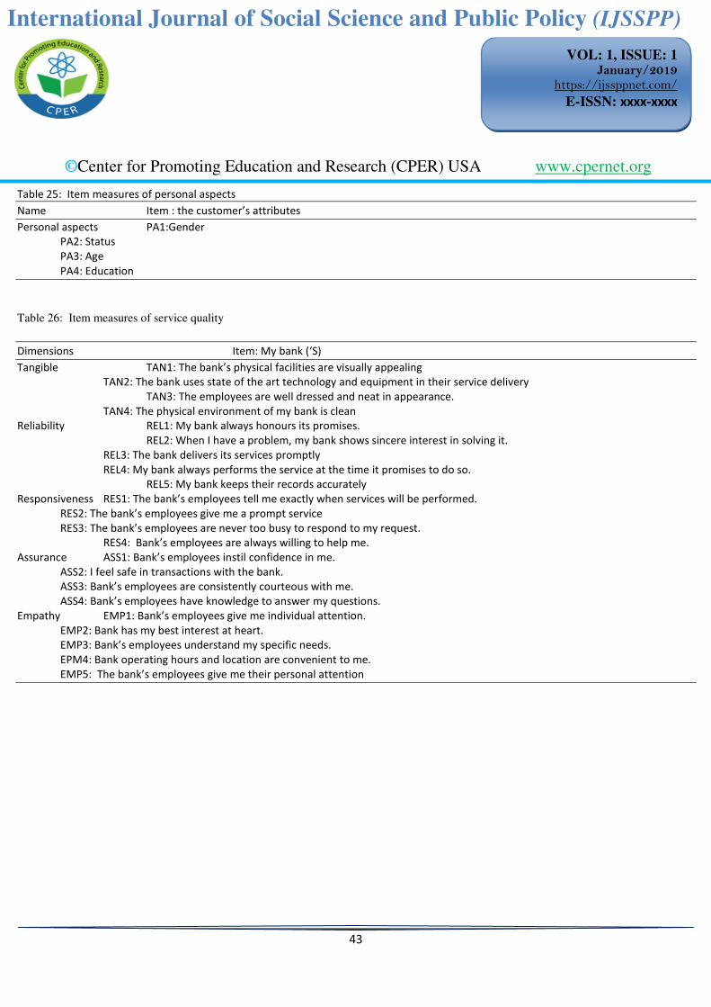
Table 25: Item measures of personal aspects

Name Item : the customer’s attributes

Personal aspects PA1:Gender

PA2: Status

PA3: Age

PA4: Education

Table 26: Item measures of service quality

Dimensions Item: My bank (‘S)

Tangible TAN1: The bank’s physical facilities are visually appealing

TAN2: The bank uses state of the art technology and equipment in their service delivery

TAN3: The employees are well dressed and neat in appearance.

TAN4: The physical environment of my bank is clean

Reliability REL1: My bank always honours its promises.

REL2: When I have a problem, my bank shows sincere interest in solving it.

REL3: The bank delivers its services promptly

REL4: My bank always performs the service at the time it promises to do so.

REL5: My bank keeps their records accurately

Responsiveness RES1: The bank’s employees tell me exactly when services will be performed.

RES2: The bank’s employees give me a prompt service

RES3: The bank’s employees are never too busy to respond to my request.

RES4: Bank’s employees are always willing to help me.

Assurance ASS1: Bank’s employees instil confidence in me.

ASS2: I feel safe in transactions with the bank.

ASS3: Bank’s employees are consistently courteous with me.

ASS4: Bank’s employees have knowledge to answer my questions.

Empathy EMP1: Bank’s employees give me individual attention.

EMP2: Bank has my best interest at heart.

EMP3: Bank’s employees understand my specific needs.

EPM4: Bank operating hours and location are convenient to me.

EMP5: The bank’s employees give me their personal attention



Documents

International Journal of Social Science and Public Policy